1

United States National PM2.5 Chemical Speciation Monitoring Networks –

CSN and IMPROVE: Description of Networks

Paul A. Solomon1,*, Dennis Crumpler2

James B. Flanagan3, R.K.M. Jayanty3, Ed E. Rickman3, RTI International

Charles E. McDade4, University of California, Davis

1. U.S. EPA, Office of Research and Development, National Exposure Research

Laboratory, Las Vegas, NV 89119, USA. solomon.paul@epa.gov.

2. U.S. EPA, Office of Air and Radiation, Office of Air Quality Planning and Standard,

Research Triangle Park, NC. 27711 USA

3. Research Triangle Institute International, Research Triangle Park, NC. 27711 USA

4. University of California, Crocker Nuclear Laboratory, Davis, CA. 95616 USA

* Corresponding author.

ABSTRACT

The U.S. EPA initiated the national PM2.5 Chemical Speciation Monitoring Network

(CSN) in 2000 to support evaluation of long-term trends and to better quantify source impacts of

particulate matter (PM) in the size range below 2.5 µm aerodynamic diameter (PM2.5; fine

particles). The network peaked at over 260 sites in 2005. In response to the 1999 Regional Haze

Rule and the need to better understand the regional transport of PM, EPA also augmented the

long existing Interagency Monitoring of Protected Visual Environments (IMPROVE) visibility

monitoring network in 2000, adding nearly 100 additional IMPROVE sites in rural Class 1 Areas

across the country. Both networks measure the major chemical components of PM2.5 using

historically accepted filter-based methods. Components measured by both networks include

2

major anions, carbonaceous material, and a series of trace elements. CSN also measures

ammonium and other cations directly whereas IMPROVE estimates ammonium assuming

complete neutralization of the measured sulfate and nitrate. IMPROVE also measures chloride

and nitrite. In general, the field and laboratory approaches used in the two networks are similar;

however, there are numerous, often subtle differences in sampling and chemical analysis

methods, shipping, and quality control practices. These could potentially impact merging the two

datasets when used to better understand source impacts and the regional nature and long-range

transport of PM2.5. This paper describes, for the first time in the peer-reviewed literature, these

networks as they have existed since 2000, outlines differences in field and laboratory

approaches, provides a summary of the analytical parameters that address data uncertainty, and

summarizes major network changes over the years. Additional papers are in preparation that will

directly compare results from colocated measurements at three urban and three rural sites and

examines if there are practical differences when using the same datasets in the same receptor

modeling application.

KEY WORDS

Fine particles; long-term trends; visibility; NAAQS support; chemical composition; sulfate;

nitrate; elemental carbon; organic carbon; trace elements; sampling and analysis methods; TOA,

thermal optical analysis, EDXRF

INTRODUCTION

Particulate matter (PM) is emitted into the air from a wide variety of anthropogenic and

biogenic sources. Particles can be emitted directly into the air (primary particles) or formed in

the atmosphere (secondary particles) from gaseous precursor emissions that nucleate to form new

particles or condense on existing particles (Seinfeld and Pandis 1998). The resulting chemical

composition of ambient particles is complex due to the many different sources of primary

particles and precursor gases and their subsequent chemical reactions and physical interactions in

air. Understanding the sources of ambient PM is important because PM has been shown to have

adverse effects on human health, degrade visibility, increase the acidity of lakes and streams,

damage materials and crops, and impact global climate (U.S. EPA 2009a). Linking sources to

ambient PM concentrations and ultimately to health effects and visibility degradation is

3

achieved, in part, by understanding the chemical composition of atmospheric PM and how it

varies temporally and spatially (Hopke 1991; Schauer et al. 1996; Hopke 2003; Brook et al.

2004; Watson et al. 2008; Solomon et al. 2008; Solomon and Hopke 2008; Solomon et al. 2012).

However, near the end of the 20th century detailed information on particle composition was

lacking for many locations around the country. To fill this gap, the U.S. Environmental

Protection Agency (EPA) and the National Park Service (NPS) established or expanded national

chemical speciation monitoring networks to collect atmospheric particulate matter at urban sites

(EPA) with a focus on linking sources to health effects (Federal Register 1997) and at rural to

pristine sites (Class I areas; NPS) with a focus on linking sources to visibility degradation

(Federal Register 1999). Of interest here are the networks related to collecting particles with

aerodynamic diameters (AD) less than 2.5 µm (fine or PM2.5) as particles in this size range have

been associated with adverse health effects and visibility degredation (U.S. EPA 2009a; Harrison

and Yin 2000; McClellan et al. 2004; Kampa and Castanas 2008; Solomon et al. 2012).

The two monitoring programs are referred to as EPA’s PM2.5 National Chemical

Speciation Network (CSN) (U.S. EPA 1999a) and the Interagency Monitoring of Protected

Visual Environments (IMPROVE) network (IMPROVE 2012a).These programs were designed

to obtain information about the spatial and temporal chemical composition of ambient fine

particles. Due to the regional nature of fine particles and the impact of regional PM on urban PM

levels (and vice versa), EPA realized the need to have a combined dataset that includes both

CSN (urban) and IMPROVE (rural) data. This combined dataset has been used to develop

effective emissions control strategies for fine particles in urban areas, including the impacts of

short- and long-range transport. While similar in design, the science and policy objectives of the

individual programs impacted their specific sampling and analysis approaches.

Variations in design and operation between these networks have resulted in potential

differences in the measured values. Understanding these differences is critical to using the

combined dataset and comparing results among sites in these two networks.

Data from these networks have been used in State Implementation Plans for over a

decade. Shortly EPA and the states will begin the PM2.5 designation and SIP process for 2018

attainment (McCarthy, 2013) and the information presented here should be useful for the

4

analyses needed to support relevant policy objectives. The specific objectives of this paper are to

1) describe the ambient measurement and laboratory chemical analysis methods employed in

these networks since 2000; 2) describe the related quality assurance procedures employed; 3)

report observed quality assurance results (e.g., blanks, minimum detection limits [MDLs], and

uncertainty); and 4) summarize changes in the networks that have occurred over the years.

NETWORK DESCRIPTIONS

EPA’s CSN Program was established through promulgation of the 1997 PM2.5 National

Ambient Air Quality Standards (NAAQS) (Federal Register 1997). The CSN began as a small

pilot network of 13 sites operating from February through July 2000. As the program grew, some

sites were specified as part of the National Air Monitoring Stations (NAMS) network designed to

track long-term trends in PM2.5 mass and composition to validate the efficacy of emission

reductions strategies and support implementation of the NAAQS (State Implementation Plans –

SIPS). These sites were initially referred to as Speciation Trends Network (STN) sites. Other

sites were specified as part of the State and Local Air Monitoring Stations (SLAMS) network

established primarily to support NAAQS implementation, with states and air quality agencies

determining the need for length of operation. Note NAMS or STN is a subset of SLAMS. Both

the STN and SLAMS chemical speciation sites are now referred to as the Chemical Speciation

Network designed to support the additional objectives of health and exposure research studies

and programs aimed at improving environmental welfare (e.g., visibility degradation).

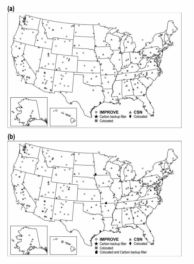
In the fall of 2000, CSN began a network expansion from its original 13 sites and by

October 2005 there were 54 STN, 181 SLAMS and Tribal sites, and 28 SLAMS that had

IMPROVE monitors (IMPROVE Protocol Sites, defined below) (U.S. EPA 2005a). All STN

sites are located in urban areas, but a few of the SLAMS sites are in non-urban areas. In early

2005, EPA began reducing the number of speciation monitors in the CSN network due to

Congressional budget reductions at EPA. In April 2006, the network consisted of 54 STN, 159

SLAMS sites, 28 SLAMS IMPROVE protocol sites, and three tribal sites (U.S. EPA 2006). In

2012, there were 51 STN, 127 SLAMS sites, and, 28 SLAMS IMPROVE protocol sites (U.S.

EPA 2013). Figure 1a indicates the CSN site locations as of 2006 and Figure 1b as of 2012.

5

The IMPROVE monitoring program was established in 1985 to aid in the development of

Federal and State implementation plans for the protection of visibility in Class I areas as

stipulated in the 1977 amendments to the Clean Air Act. The network began collecting samples

in 1988 with 20 sites (Eldred et al., 1990). At that time, IMPROVE had a long-term goal of

monitoring for regional haze in all visibility-protected Federal Class I areas as stipulated in the

1999 Regional Haze Rules (Federal Register 1999). By 1999, the IMPROVE network had

increased to 30 IMPROVE sites in Class I areas and 40 IMPROVE Protocol sites, that is, sites

that are part of the IMPROVE database, but are funded separately by a Federal Land Manager,

state agency, or other entity. IMPROVE sites and IMPROVE Protocol sites are operationally

identical in every respect, the only differences being their source of funding and, in some cases,

their proximity to Class I areas. With implementation of the Regional Haze Rule and EPA’s

desire to combine CSN and IMPROVE data the IMPROVE network was expanded by spring

2004 to 110 IMPROVE sites in Class I areas and 57 Protocol sites. All but a few IMPROVE

sites are located in Class I Areas where aerosol concentrations are typically much lower than

urban levels. Twenty-eight of the IMPROVE Protocol sites are operated at state SLAMS sites, as

noted above, and these SLAMS data are also included in EPA’s Air Quality System (AQS) (U.S.

EPA 2012a).The number of IMPROVE sites has remained roughly the same since 2004. Figure

1a indicates the IMPROVE site locations as of 2006 and Figure 1b as of 2012.

Similar time-integrated, filter-based approaches and laboratory analytical methods are

used in both networks; each measuring PM2.5 mass and its major components including sulfate,

nitrate, ammonium (CSN only), organic carbon and elemental carbon (OC, and EC,

respectively), and a number of elements found in crustal and industrial sources including, but not

limited to Mg, Al, Si, S, Ca, Ti, V, Fe, and Zn. However, due to the different policy objectives of

the two networks, differences, sometimes subtle in nature, exist between the sampling and

analytical procedures employed (IMPROVE 2012a; Koutrakis 1998; Koutrakis, 1999; U.S. EPA

1999a). Choices in specific measurement and analytical methods also were made based on

funding, available technology, and the desire for long-term monitoring (Koutrakis 1998;

Koutrakis, 1999; U.S. EPA 1999). Current information relating to CSN and IMPROVE

measurements is provided at their respective websites (IMPROVE 2012a; U.S. EPA 2012b).

6

Tables 1-7 present various aspects of the two measurement programs showing the subtle

and not so subtle differences among the methods employed. Despite these many differences,

results from the two networks typically agree well for high-concentration and non-labile species

such as sulfate.

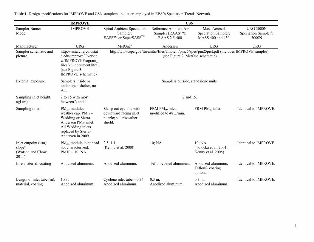
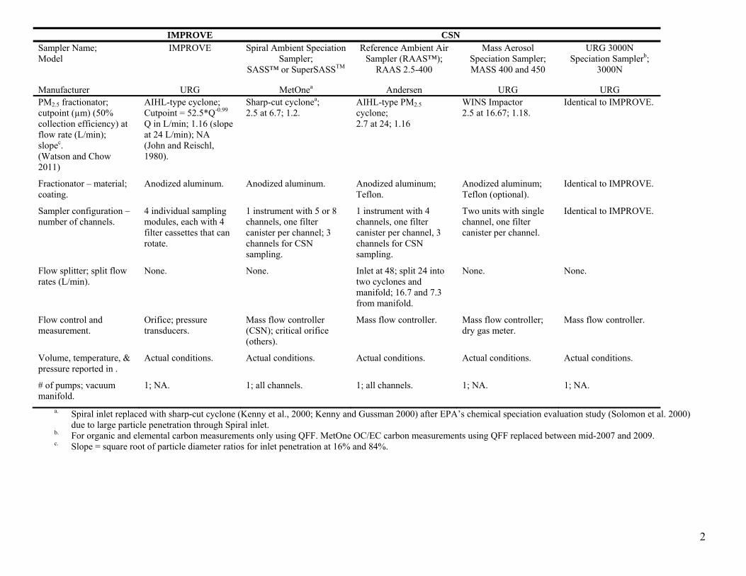
Table 1 provides design specifications for IMPROVE and the three STN samplers. See

Figures 2 and 3 for sampler schematics.

Table 2 summarizes analytical laboratory methods by filter type and chemical

component.

Table 3 summarizes filter media, acceptance tests, and sample preparation procedures.

Table 4 lists the original CSN and current CSN and IMPROVE operating conditions for

the OC/EC analysis protocols.

Table 5 describes denuders used to remove acidic gases in the channel that contains the

nylon filter. See Figures 2 and 3.

Table 6 provides a summary of sample handling, shipping conditions, holding times, and

laboratory storage requirements.

Table 7 describes the filter characteristics, flow rates, and face velocities for both

networks.

Sampling Methods

CSN and IMPROVE samplers both employ filter -based time-integrated (24-hr average)

sampling approaches that can provide a nearly complete mass balance via subsequent laboratory

chemical analysis of the collected PM. For the collection of nitrate, both networks use denuders

and reactive nylon filters to minimize sampling artifacts caused by nitrate volatilization (Hering

et al. 1988; Hering and Cass 1999). Carbon artifacts are accounted for by using various blank

correction approaches (Kim et al. 2005; Chow et al. 2008; Watson et al. 2009; Chow et al. 2010;

Maimone et al. 2011), as discussed below. Therefore, these samplers are designed to minimize

sampling artifacts for nitrate while allowing flexibility for estimating organic carbon artifacts.

7

Additional details regarding CSN and IMPROVE samplers are given in Table 1 and in standard

operating procedures (RTI 2013; IMPROVE 2012b).

CSN. Three prototype and commercially available chemical speciation samplers were

initially evaluated for use in the CSN (Solomon et al. 2000; Solomon et al. 2003) and results are

summarized briefly below. The prototype samplers were the MetOne SASS (Spiral Ambient

Speciation Sampler), the URG MASS (University Research Glassware Mass Aerosol Speciation

Sampler), and the Thermo Anderson RAAS (Reference Ambient Air Sampler). Photographs and

schematics of the three samplers can be found in the literature (Solomon et al. 2000) and on the

EPA’s Technology Transfer Network web site (U.S. EPA 2012c). All three samplers, one at each

of the three sites, also were included in the 2001 – 2003 CSN-IMPROVE comparison, which

will be the focus of a subsequent paper. R&P samplers (Model 2300; Rupprecht & Patashnick,

Co., now Thermo-Scientific) were not available at the time of initial testing, and therefore were

not included in the CSN-IMPROVE comparison study. In addition, few CSN sites used R&P

samplers (7 % in 2006, none in 2012) and they will not be discussed in this paper.

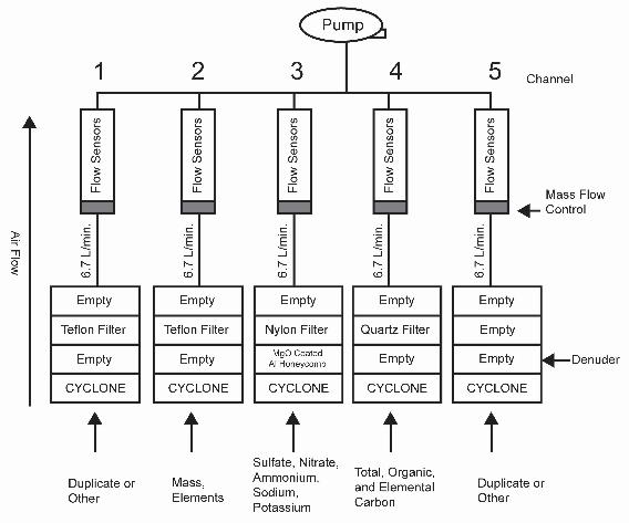
Figure 2 shows a schematic drawing of the MetOne sampler, which, as of January 2007

was used at 84% of the CSN sites. Given the high percentage of MetOne samplers at this time,

EPA made a decision to convert the entire network to MetOne samplers for collecting PM on the

Teflon and nylon filters. This conversion was completed by mid-2009. The original MetOne

sampler consisted of five sampling channels. A second version (Super SASS) was developed

with 8 channels to allow for sequential sampling, which as of the beginning of 2014 has not been

implemented. In both the SASS and the Super SASS, each channel operates at a flow rate of 6.7

L/min and each has its own sampling module designed for 47 mm diameter filters. In the SASS,

three channels (SuperSASS, six channels - two sets used for sequential sampling) are normally

used for CSN sampling, one each for Teflon, nylon, and quartz-fiber filters (QFFs). In both

samplers, only three channels employ mass flow controllers allowing flow control to within 1%

or better although corrections need to be made for variations in temperature and pressure to

obtain volumetric flow. The additional channels in both samplers employ critical flow orifices

for flow control (Baker and Pouchot 1983; Hinds 1999) and are available for replicate sampling

or other uses. Each sampling module uses a sharp cut cyclone (SCC 2.141) that has similar

performance characteristics to the EPA Well Impact Ninety-Six (WINS) impactor used in the

8

PM2.5 FRM (Peters et al. 2001). Sampling modules consisting of the filter cassettes and denuders

are shipped to and from the laboratory with each sample.

The Anderson RAAS has four available flow channels, two each under two identical

cyclone/manifold sets. The total flow rate through the inlet is 48 L/min and through each

manifold is 24 L/min. Like the SASS, three channels are used for CSN sampling. The fourth

channel is available for other needs, such as collecting a replicate sample. One channel under

each manifold operates at 16.7 L/min and each includes a Teflon filter, one used for mass and

elemental analysis, the other for replicate measurements. The second channel under each

manifold operates at 7.3 L/min. One channel includes the nylon filter, which is preceded by an

MgO coated annular denuder to remove acidic gases and the other includes a QFF. All channels

employ mass flow control and each use 47 mm diameter filters. Sampling modules consisting of

the filter cassettes and denuders are shipped to and from the laboratory with each sample.

The URG MASS 400/450 sampling system uses two standalone samplers operating at

16.7 L/min, each with mass flow control. Each sampler includes a filter holder for 47 mm

diameter filters and both samplers employ the WINS impactor identical to that used in the PM2.5

FRM program. The MASS 450 contains a single QFF for OC and EC analysis. The MASS 400

includes a sodium carbonate coated annular denuder upstream of the Teflon – nylon sequential

filter pack. Nitrate that can volatilize from the front Teflon filter during sampling is captured and

measured on the backup nylon filter (Hering and Cass 1999; Solomon et al. 2000). Therefore, for

this sampler only, nitrate is the sum of nitrate measured on the Teflon front and nylon backup

filter. Mass, trace elements, and then ions in that sequence are measured on the Teflon filter. As

a result, lower nitrate values are observed on the URG relative to the other samplers, since nitrate

can volatilize off the Teflon filter during analysis by energy-dispersive x-ray fluorescence

(EDXRF), which occurs prior to analysis for ions (Solomon et al. 2000; Solomon et al. 2003, Yu

et al. 2006).

Starting in February 2007, CSN started transitioning sampling on QFF for carbonaceous

components to the URG 3000N sampler (U.S. EPA 2007b; U.S. EPA 2012e). This sampler is

virtually identical to the sampler used by IMPROVE for collecting OC and EC, except the

critical orifice was replaced with a mass-flow controller and how filters are shipped between the

9

laboratory and field as described later. QFF collected by the URG 3000N are analyzed by the

IMPROVE_A method. This transition was completed by late 2009 and all carbon analyses are

now done using the URG 3000N/IMPROVE_A protocols.

CSN samplers are operated by state, local, and tribal agency personnel. Research

Triangle Institute International (RTI, Research Triangle Park, NC) is currently the laboratory

responsible for filter preparation, shipping, chemical analysis, and database management for all

STN sites. Primarily RTI, but others also are responsible for these tasks at SLAMS sites. These

include state laboratories in California, Oregon, Nevada, the two former for California and

Oregon sites and the latter for SLAMS sites in the State of Texas. Samples are collected once

every three days at STN sites and once every three or six days at SLAMS sites, the latter

schedule is defined by the state, local, or tribal agency responsible for the sampling site. Samples

collected by CSN can remain on the sampler for up to 3 days (U.S. EPA 2012d). All CSN filters

remain in their sampling modules or filter holders, which are sealed at both ends, placed in

sealed anti-static Ziploc plastic bags, and shipped in coolers with blue ice by overnight carrier

service. The temperature target at receipt is not to exceed 4° C, although this has been frequently

exceeded by a few degrees, particularly in the summer months. A flag is noted in the database

for samples arriving at greater than 4° C. Before and after sampling filters remain in clear

polystyrene Petri dishes (Millipore PetriSlides™ or equivalent) that are stored at reduced

temperatures (< 0° C). Petri slides are used as they come from the manufacturer, without further

cleaning but are visually inspected for debris or deformities. Petri slides are not reused in CSN.

Additional details about the CSN sampling and analysis protocols can be found at the AMTIC

web site (U.S. EPA 2012b) .

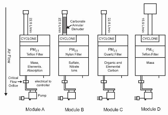
IMPROVE. All IMPROVE and IMPROVE Protocol sites use the same sampler design as

shown in Figure 3 and summarized in Table 1. The sampler consists of three separate modules

for PM2.5 and a fourth module for PM10. Each module uses a critical orifice to control flow, and

contains 4 solenoid valves and corresponding filter holders to allow for a blank sample to be

collected and/or for sequential operation. One of the PM2.5 modules uses a 25 mm diameter

Teflon filter for mass, light absorption, and trace elements, a second uses a 37 mm nylon filter

for ions, which is preceded by a sodium carbonate coated Al annular denuder; and a third uses a

10

25 mm QFF for organic and elemental carbon. Finally, a 25 mm Teflon filter is used in the PM10

module for PM10 mass.

IMPROVE samplers are operated by local operators at each site, often National Park

Service (NPS) personnel or state agency personnel. Currently, IMPROVE samples are collected

once every three days, to be consistent with CSN, whereas prior to 2000 they were collected only

on every Wednesday and Saturday. Filters are allowed to be left on the sampler for up to 7 days

after collection (IMPROVE 2012c). IMPROVE filters are prepared at UC Davis with the

exception of QFF filters that are prefired at the Desert Research Institute (DRI) and shipped to

UC Davis prior to sampling. Filters are sent between the field sites and UC Davis in their

sampling cassettes sealed in Ziploc plastic bags at ambient temperature. Shipping is by UPS or

by standard U.S. mail in plastic containers designed for durability but not thermal stability.

Following sampling, QFF filters for organic carbon analysis are shipped between UC Davis and

DRI at reduced temperatures, where the QFF are stored below 0° C and analyzed. Nylon filters

are shipped in Petri dishes at ambient temperatures by US mail to RTI for analysis of ions. Petri

dishes are used initially as they come from the manufacturer, without further cleaning but are

visually inspected for debris or deformities. Used Petri slides for nylon filters are washed in

ethanol and reused with no contamination observed. Other Petri slides are not reused. Additional

details are given in the IMPROVE Quality Assurance Project Plan (Flocchini et al. 2002) and in

IMPROVE standard operating procedures (IMPROVE 2012b).

Analytical Methods

Similar analytical methods are employed by the CSN and IMPROVE monitoring

programs, as summarized in Table 2. PM2.5 mass is measured gravimetrically by weighing

conditioned filters before and after sampling. Water soluble ionic species are extracted from the

nylon filter (the Teflon filter in the case of the URG MASS samplers) and determined by ion

chromatography (IC). Organic and elemental carbon are determined by thermal optical analysis

(TOA) from QFF and up to 48 trace elements have been measured by EDXRF from the Teflon

filter used first for mass determination. Organic species are not measured routinely in either

network. Numerous subtle and not so subtle differences exist between the methods employed in

11

the two networks with regards to the analytical methods, preparation procedures, sample storage,

shipping, and methods for determining and correcting for blanks and interferences.

Additional details for the CSN analytical methods are given in Solomon et al. (2001) and

U.S. EPA (1998) and in specific laboratory standard operating procedures (SOPs) for mass and

chemical speciation (RTI 2008; RTI 2009a-f, RTI 2011)

IMPROVE mass and chemical analyses are conducted at UC Davis, RTI, and DRI. Mass,

elemental, and light absorption analyses are conducted at UC Davis, ions are analyzed at RTI,

and OC/EC analysis is at DRI. Additional details for IMPROVE analytical procedures are given

in the IMPROVE Quality Assurance Project Plan (Flocchini et al. 2002) and standard operating

procedures (IMPROVE 2012b).

The remainder of this section gives brief summaries of the methods employed by both

programs and addresses some of the differences.

Acceptance Testing. Acceptance testing of new filter lots is conducted to ensure filter

quality and consistency over time. Acceptance tests and sample preparation procedures are

summarized in Table 3 for both networks (DRI 2005; RTI 2011, IMPROVE 2012d). Differences

between acceptance testing protocols exist but likely make little difference in the measurements

since quality assurance procedures require the collection and analysis of blanks throughout the

sample and analysis process.

For CSN, Teflon filters are visually inspected and a subset analyzed for trace elements. If

the average blank level (µg/cm2) for any element is greater than three times the variability (3σ)

of the MDL, then an intercept is included in the EDXRF calibration equation for that element.

The same intercepts are used until a new batch of filters is received; the 10 filters do not

constitute a fixed percentage of filters.

CSN nylon filters received from the manufacturer are washed for 24-hr in several

changes of DI water (RTI 2009b). The washing solution for 2 out of every 100 filters is analyzed

for ionic species to ensure they are below acceptance levels as given in Table 3 (U.S. EPA 2000)

12

CSN QFF are heat treated to remove OC associated with new filters from the

manufacturer (Table 3). This process lowers the blank level to below the MDL. However, while

heat treating removes the initial OC artifact, QFF medium continues to sorb organic gases until

reaching pseudo-equilibrium. The overall artifact is both passive and active and depends on the

sampled volume and several other factors and can reach the equivalent of 4 µg /m3 for CSN

filters sampled with the MetOne sampler (McDow and Huntzicker 1990; U.S. EPA 1998;

Solomon et al. 2000; Turpin et al. 1994; Turpin et al. 2000; Maimone et al. 2011).

All Teflon filters used in IMPROVE are visually inspected for imperfections. For each

new lot, the pressure drop at 22.8 L/min is checked in the laboratory using a manometer and a

subset (10) filters are weighed to verify the correct weight range of each new batch of filters.

Finally, selected filters are analyzed by EDXRF, Proton Elastic Scattering Analysis (PESA,

discontinued January 2011), and Hybrid Integrating Plate/Sphere analysis (HIPS) to check for

contamination.

New lots of IMPROVE nylon filters also are visual inspected and the pressure drop

measured similar to the Teflon filters. A subset of filters is analyzed for sulfate, nitrate, nitrite,

and chloride contamination to ensure they are below acceptance levels as given in Table 3

IMPROVE QFF filters are visually inspected and heat treated to reduce initial blank

levels similar to CSN. However, while filters in both networks are heated at the same

temperature the time is slightly different as well as how the filters are treated and stored after

heating (Table 3). A subset of filters is selected after the initial cleaning and analyzed for OC

and EC to ensure blank vales are within acceptable levels.

Mass. Gravimetric analysis is used in both networks to obtain PM2.5 mass (Table 2).

IMPROVE also measures PM10 mass by this method. An estimate of coarse particle mass

(particles in the size range between 2.5 and 10 µm AD) can be obtained by difference between

simultaneously measured PM10 and PM2.5 mass concentrations. Collection of PM10 also provides

a quality control check on the PM2.5 mass since PM2.5 mass must always be less than the PM10

mass. CSN Teflon filters used to obtain PM mass are equilibrated for 24-hr before and after

weighing to minimize mass variation due to particle bound water (Table 2). CSN adheres to the

FRM PM2.5 mass analysis protocol to obtain concentrations in units of µg/m3 (Federal Register

13

1997; U.S. EPA 1998; RTI 2008). IMPROVE equilibrates Teflon filters for mass at a slightly

different temperature and RH range but only for several minutes (Table 2). Unpublished

laboratory tests of exposed Teflon filters at UC Davis as well as EPA audits have demonstrated

that filters collected at rural and remote monitoring sites appear to equilibrate to laboratory

conditions within a few minutes (IMPROVE 2012d).

Ions. Ion chromatography is used to determine concentrations of major water soluble ions

from the PM collected on the nylon filter in both networks (Table 2). Ions also were measured on

the Teflon front filter collected by the URG MASS. In this case, total nitrate equaled the sum of

nitrate measured on the Teflon front filter and nylon backup filter. Both networks measure

sulfate, and nitrate. CSN also measures ammonium, sodium, and potassium ions whereas

IMPROVE also measures, chloride and nitrite ions and estimates ammonium based on fully

neutralized sulfate ((NH4)2SO4) and nitrate (NH4NO3). RTI analyzes filters for ions for both

networks (RTI 2009c, RTI 2009d; IMPROVE 2005). The same IC conditions are used in both

networks and both networks extract nylon filters in DI water, except for the CSN URG nylon

backup filter, which is extracted in IC eluent. Slightly different extraction conditions are used

between the networks. IMPROVE extracts at room temperature, whereas CSN extracts at

reduced temperatures to stabilize semi-volatile species, such as nitrate and ammonium. However,

high extraction efficiencies have been demonstrated for both programs (Clark 2002a).

Differences in ion analysis approaches are summarized in Table 2. Use of nylon as the collection

medium results in a potential negative artifact for ammonium (Solomon et al. 2000; Yu et al.

2006).

Carbon. Thermal optical analysis is used to determine concentrations of organic and

elemental carbon in both networks (Table 2). The two programs initially used different

temperature protocols and optical approaches, the latter to correct for OC charring. The

different temperature protocols are shown in Table 4. They different optical approaches occur

during the He temperature steps (Chow et al. 1993; Chow et al. 2001; Chow et al. 2004; Chow et

al. 2005a; Chow et al. 2007; Peterson and Richards, 2002; Watson et al. 2005; RTI 2009e).

Beginning in 2008 and finishing in 2009, CSN transitioned to the IMPROVE_A analysis

protocol to obtain consistency between the networks. Prior to 2009, CSN used thermal optical

transmittance (TOT) (Peterson and Richards, 2002), whereas IMPROVE used thermal optical

14

reflectance (TOR) (Chow et al. 1993). Differences due to use of TOT versus TOR have been

observed (Chow et al. 2004). Beginning with samples collected in January 2005, IMPROVE

provides both TOR and TOT results (DRI 2005; Chow et al. 2007). Several studies have been

conducted comparing the IMPROVE, CSN, and in some cases other protocols for OC and EC

(Chow et al. 2001; Schmid et al. 2001; Conny et al. 2003; Chow et al. 2004; Watson et al. 2005;

Cheng et al., 2011).

The variation between the two approaches for OC measured on typical urban and rural

samples ranges from about 10-30%; for EC the difference can be up to a factor of 2 or more for

the different analytical protocols used in the comparison studies (Solomon et al. 2000; Chow et

al. 2001; Schmid et al. 2001; Solomon et al. 2003; Chow et al. 2004; Watson et al. 2005; Chow

et al. 2008; Cheng et al. 2011). Total carbon (TC), equal to the sum of OC and EC, usually

agrees to within 10-15%. Agreement for TC indicates that differences in the analytical

approaches for OC and EC are likely due to how the two protocols determine the split between

OC and EC and/or correct for OC charring (i.e., TOT vs. TOR).

IMPROVE also analyzes the PM2.5 Teflon filters for optical absorbance (1/m) of the

particles collected on the filters by HIPS (Bond et al. 1999). Optical Absorbance is not measured

in CSN. Absorbance by the collected particles is important for estimating light extinction, a

critical parameter for quantifying visibility and IMPROVE’s primary policy objective. The

absorbance is divided by an empirically determined absorptivity coefficient (m2/μg) to convert it

to black carbon (BC) in concentration units of µg/m3 although a range of values exist for this

conversion (Bond and Bergstrom 2006). BC measured optically is similar to but not the same as

EC measured thermally (Fehsenfeld et al. 2004). In HIPS, the filters are exposed to light at 633

nm wavelength from a He (Ne) laser and the light transmitted through the sample is collected

with a photodiode detection system. This measurement provides a quality control check on the

absorptivity coefficient and/or elemental carbon measurements, the latter since elemental carbon

is typically the predominant light absorbing particulate species in the atmosphere.

Trace Elements. Energy dispersive X-ray fluorescence is used by both programs to

quantify trace elements (Na – Pb) in PM2.5 collected on Teflon filters (Table 2) (RTI 2009f;

IMPROVE 2012e). IMPROVE has also used PESA to measure hydrogen (IMPROVE 2012f),

15

but this analysis was discontinued in 2011 for budgetary reasons. The CSN program initially

reported 48 elements (reduced to 33 elements in 2009), while IMPROVE reports 25, focusing

only on those that are reliably measured above the MDL of the instrument. As noted in Table 2,

prior to December 2001, IMPROVE used Proton Induced X-ray Emission (PIXE) for Na-Mn and

EDXRF for Fe-Pb (IMPROVE 2006). The switch to only EDXRF provides lower MDLs for

most elements of interest, as well as ensures better sample preservation for reanalysis (PIXE can

damage filters). Still, EDXRF is not sufficiently sensitive for many of the elements measured by

both networks, so typically only about 10-15 elements are reported above their detection limit for

the primarily urban CSN and about 15-20 elements for the primarily rural IMPROVE network.

The higher filter loading (volume sampled/area of filter, m3/cm2) combined with differences in

analytical parameters result in better ambient MDLs for IMPROVE, which allows more species

to be measured above their detection limits.

Different EDXRF instruments are used by the two programs. In addition, to obtain

sample throughput, CSN uses two EDXRF instruments and laboratories, one operated by RTI

and the other by Chester LabNet (Portland, OR).

The RTI EDXRF and Chester LabNet laboratories analyze filters from the long-term

trend networks (STN and NCORE; U.S. EPA 2005c; Scheffe et al. 2009). Filters collected by

California, Oregon, and Texas are analyzed by state and local district laboratories (California Air

Resources Board, DRI, and Oregon Dept. of Environmental Quality, South Coast Air Quality

Management District) (Smiley 2013). RTI uses Thermo Scientific QuantX EDXRF analyzers, each

equipped with a high flux rhodium anode X-ray tubes and an electronically cooled lithium-

drifted silicon detector (RTI 2009f). Elements are analyzed using one of five different excitation

conditions defined by different anode operating conditions and X-ray filters. Chester LabNet

uses similar anodes and detector systems, though there are slight differences in the excitation

conditions relative to the CSN laboratory (Chester 2009). While each instrument is calibrated to

meet QC criteria individually, between-instrument and between-laboratory variations can

introduce additional uncertainty in the CSN EDXRF results (Smiley 2013).

Prior to 2011 IMPROVE used a Cu anode EDXRF system to quantify elements with

atomic weights from Na through Fe, and a Mo anode for elements with atomic weights from Ni

16

through Pb. Prior to 2005 the Cu anode system utilized a helium purge to remove air around the

sample thus minimizing interferences due to the argon spectral peak. Beginning with samples

collected in January 2005, a vacuum system was introduced because He diffused through the Be

window of the SiLi detector, changing the calibration and eventually destroying the detector. A

second (nominally identical) vacuum-based EDXRF system was introduced in October 2005 to

increase laboratory capacity. In 2011 the aging Cu and Mo anode systems were replaced by

PANalytical Epsilon 5 EDXRF instruments. With the Epsilon 5 system elements are analyzed

using one of seven different excitation conditions defined by different exposure times and

secondary X-ray targets. Data advisories addressing the impacts of changes in EDXRF hardware

and procedures are available from IMPROVE (IMPROVE 2012g). CSN has similar information

available in annual data reports (http://www.epa.gov/ttn/amtic/specdat.html), special study

reports (TTN 2012a), and CSN the newsletters (2004 – 2009;

http://www.epa.gov/ttn/amtic/spenews.html).

Self-absorption corrections for particle size and filter loading were applied by both

networks but a detailed description of the approaches employed are beyond the scope of this

paper. Self-absorption corrections for IMPROVE were applied to the legacy EDXRF data prior

to 2011 (Dzubay and Nelson 1975; IMPROVE 1997). A homogeneously distributed sample

deposit on the filter is assumed as well as incorporating particle-size and mass loading effects.

Self-absorption is strongest for the lightest elements such as Na and Al decreases substantially

for heavier elements. The correction was discontinued with the introduction of the new

PANalytical Epsilon 5 instruments, which provide much improved sensitivity for the lighter

elements where self-absorption is greatest.

Similar to the IMPROVE methodology, the CSN self-absorption assumes a homogeneous

and uniformly distributed sample and incorporates particle-size and mass loading effects. The

CSN self-absorption procedure is a modification of the protocol used by EPA with the Thermo

Scientific QuantX spectrometers (Dzubay and Wilson 1974; U.S. EPA 1999c). The procedure

corrects for signal loss due to scattering and absorption by calculating an absorption correction

factor that compensates for measured intensities in a homogeneous sample relative to a thin-film

standard. Self-absorption corrections vary by sample composition, but in general are similar to

those in the IMPROVE network.

17

EDXRF round-robin performance evaluations of CSN and IMPROVE laboratories were

conducted by EPA (Smiley 2013). Comparability between laboratories for many high

concentration elements (e.g., elements, Fe, Ca, K, Zn) was considered acceptable. The poorest

agreement was for Al and Na. This is expected, since low molecular weight elements have a

relatively poor instrument response and typically require correction for self-absorptions, both of

which can lead to higher uncertainty for these elements. Furthermore, the two networks use

different approaches to correct for self-absorption as noted above, though the uncertainties seem

to agree reasonably well (U.S. EPA 2011).

MEASUREMENT UNCERTAINTY

As in all measurement programs, measurement uncertainty in CSN and IMPROVE

includes both random and systematic errors. Precision is a measure of random errors, which is

usually determined for the combined field and laboratory operations by collecting colocated

replicate samples or by propagating individual instrument errors through all components of the

measurement process. Accuracy provides a measure of systematic error, which is a measure of

the difference between a ‘true value’ and the estimate of the true value based on the

measurement. Overall measurement accuracy is not possible for most PM measurements since

traceable standards applied in the field are not available (Fehsenfeld et al. 2004). However,

analytical laboratory measurement accuracy is reported and general values are provided in

Fehsenfeld et al. (2004). Factors affecting overall uncertainty include the coupled effects of

measurement precision, interferences, measurement and analysis artifacts, and MDL. Estimating

these parameters is critical to understanding the validity of a measurement.

A number of studies have been conducted to better understand uncertainty and factors

influencing uncertainty in CSN and IMPROVE measurements. A selection of papers published

since about 2000, i.e., most relevant to the current networks, are cited herein and provide

information about uncertainties associated with measuring the chemical components of PM;

however, a comprehensive review and evaluation of results published is beyond the scope of this

manuscript. Studies examined uncertainty issues in only one network or the other; whereas

others examined it between networks. These studies include the initial CSN intercomparisons

(Solomon et al. 2000; Coutant and Stetzer 2001; Solomon et al. 2003), estimating the overall

18

measurement uncertainty for mass or one or more chemical components for CSN and IMPROVE

(Solomon et al. 2000; Chow et al. 2001; Solomon et al. 2003; Ashbaugh et al. 2004a-b; Chow et

al. 2004; Watson et al. 2005; White et al. 2005; Yu et al. 2006; Smiley 2013; Hyslop and White

2008b), and estimating different uncertainty components (blanks, MDL, sampling artifacts) for

OC, mass, ions, and elements by EDXRF (Iyer et al. 2000; Gutknecht et al. 2001; Kim et al.

2001; Lewtas et al. 2001; Fehsenfeld et al. 2004; Subramanian et al. 2004; Gego et al. 2005; Kim

et al. 2005; Gutknecht et al. 2006; Zhao et al. 2006; Chow et al. 2008; Hyslop and White 2008a;

Watson et al. 2009; Chow et al. 2010; Gutknecht et al. 2010; Cheng et al. 2011; Maimone et al.

2011; Malm et al. 2011). Several special EPA Office of Air Quality Planning and Standards

(OAQPS) studies also were conducted to examine sampling artifacts associated with QFF

medium caused by a specific filter cassette (Clark 2002b); the effect of QFF filter type

(manufacturer) for collection and analysis of OC and EC (Peterson et al. 2007), the extraction

efficiency of ions from nylon filters using water rather than a basic solution, the latter as used

historically (Clark 2002a; Clark 2003); examining the efficacy and capacity of different diffusion

denuder coatings for the removal of acid gases (Fitz 2002); and the reanalysis of existing filters

for independent inter-laboratory comparisons and sample storage stability testing (Coutant and

Stetzer 2001; TTN 2012b). Approaches used to estimate uncertainty for the CSN and IMPROVE

networks based on CSN and IMPROVE measurements are summarized in the next few sections,

including estimates for sampling artifacts, blank estimates, and MDL. Data completeness, an

important parameter with regards to data validity also is summarized for both networks.

CSN AND IMPROVE QUALITY ASSURANCE PROGRAMS

A rigorous quality assurance program (U.S. EPA 1998; Flocchini et al. 2002; U.S. EPA

2012d; U.S. EPA 2012f; Smiley 2013), as conducted by EPA for CSN and IMPROVE, helps to

ensure the delivery of high quality data with known uncertainty to data users, such as state and

local agencies, the NPS, and other stakeholders. These groups use these data to develop

strategies to protect public health and welfare from the adverse effects of air pollution. Quality

assurance helps to identify factors that can increase uncertainty, and once minimized, ensures

those uncertainty levels are maintained by establishing a set of performance criteria or data

quality objectives (DQOs) (U.S. EPA 1999b; White et al. 2005). For historical purposes, Table 8

19

lists the performance criteria recommended for the CSN and IMPROVE networks in developing

the joint networks (Koutrakis 1999; Solomon et al. 2000, Solomon et al. 2003).

QA Field and Laboratory Programs

EPA conducts system and performance audits for field and laboratory measurements in

accordance with EPA’s Quality Assurance Project Plans for CSN and IMPROVE (U.S. EPA

2000; Flocchini et al. 2002; U.S. EPA 2012f). Field and laboratory audits include both system

and performance audits. Laboratory audit results are available at U.S. EPA (2011). Field audit

results are not currently posted for public access although RTI is beta testing an input to EPA’s

Air Quality System (AQS) for field audit results. AQS is EPA's repository of ambient air quality

data.

Field Audits. Quality Assurance Project Plans (QAPP) for CSN (U.S. EPA 2000) and

IMPROVE (Flocchini et al. 2002) field sampling operations provide guidance and detailed

direction on field audits and procedures. The updated CSN QAPP (U.S. EPA 2012f) and

IMPROVE QAPP (IMPROVE 2002) are currently the overarching quality assurance documents

for CSN and IMPROVE’s external EPA field audits. Additional individual guidance documents

are available for CSN (U.S. EPA 2012b) and IMPROVE (IMPROVE 2012e). A limited number

of independent field audits were conducted by EPA’s Office of Radiation and Indoor Air

(ORIA), Radiation and Indoor Environments National Laboratory (R&IENL), Las Vegas, NV

(western sites) and by EPA’s Office of Air Quality Planning and Standards (OAQPS; eastern

sites). Based on guidance in the CSN QAPP (U.S. EPA 2000), comprehensive field audits were

to occur on approximately 25% of the CSN sites annually. This percentage was never realized

due to reductions in 2001 in EPA’s travel budget so EPA began to aggressively train State,

Local, and Tribal (SLT) agency and NPS personnel to conduct the field audits. SLT and NPS

audits are conducted by groups within these organizations that are independent of field sampling

operations. Audits by EPA personnel were eliminated by 2010. , which

Field systems audits consist of six parts; 1) identifying organization and responsibilities

for site operations, 2) evaluating safety, 3) validating that site location and samplers meet 40

CFR Part 58, Appendices A and E siting criteria, 4) confirming that the monitoring area and

logbooks are maintained, 5) validating proper sample handling and chain of custody, and 6)

20

ensuring that proper procedures are being followed for onsite storage and shipping. Performance

audits, conducted simultaneously with systems audits, consist of validating MQOs (Table 9; U.S.

EPA 2012f) against traceable reference standards.

Laboratory Audits. EPA’s Office of Radiation and Indoor Air (ORIA), National

Analytical Radiation Environmental Laboratory (NAREL) provides annual performance

evaluation (PE) samples to laboratories that analyze CSN and IMPROVE filters. These samples

consist of filters and solutions with known quantities of the analyte spiked onto the filters using

NAREL laboratory analysis results as the reference (U.S. EPA 2012b). NAREL also collects

colocated ambient filters using the SuperSASS, which are then distributed with blank filters for

analysis of mass (Teflon filters), ions (nylon and Teflon filters), carbon (QFF), and trace

elements (Teflon filters). Separate anion and cation solutions of known concentrations and

uncertainty also are provided for IC analysis. NAREL also sends performance audit (PA)

samples to the analytical laboratories. These include NIST traceable metal weights for

gravimetric analysis and sucrose spiked QFF for TOA analysis. For trace elements, Teflon filters

with ambient PM are circulated that have been independently analyzed by the EPA’s National

Exposure Research Laboratory’s (NERL) EDXRF facility. Once the audited laboratories have

analyzed the filters, they are returned to NERL for reanalysis to ensure that the concentrations of

elements on the filters have not changed due to handling and shipping. On-site laboratory

technical systems audits (TSA) also are conducted by NAREL personnel. Results from system

and performance laboratory audits are available (U.S. EPA 2011).

Artifact and Blank Corrections

A blank is a relatively constant error affecting the measurement value and can be

evaluated with a control sample in which all steps of the analysis are performed in the absence of

the actual sample. The blank value is then applied as a correction (subtraction) to the

measurement. Three types of blank filters have been collected for these programs: laboratory,

trip, and field. Each type helps to identify potential areas of contamination and is part of the

standard EPA quality assurance/quality control programs.

Artifacts can be positive or negative and are variable errors that affect the measurement

and may not always be properly evaluated with a blank. When sampling atmospheric particles,

21

artifacts are typically due to collection of gases on a sampling substrate or volatilization of

sample already collected. Determining the impact of an artifact on the measurement may be

complicated as noted below (e.g., Chow 1995; Hering and Cass 1999; Solomon et al. 2000;

Turpin et al. 2000; Kim et al. 2001; Pang et al. 2002; Ashbaugh et al. 2004a-b; Subramanian et

al. 2004; Chow et al. 2005a-b; Kim et al. 2005; White et al. 2005; Yu et al. 2006; Watson et al.

2009; Chow et al. 2010; Maimone et al. 2011). For example, issues associated with sampling OC

on QFFs include adsorption and absorption on both collected particles and quartz-fiber filter

material (positive sampling artifacts) and may occur passively during storage, transport, and

handling or actively during sampling. Conversely, volatilization of semi-volatile organic

compounds (SVOC) from collected particles (negative sampling artifacts) can occur during

sampling with a likely dependence on flow rate or pressure drop, temperature, and RH (McDow

and Huntzicker 1990). Negative artifact also can occur throughout the transport and storage

processes after collection. Both positive and negative OC sampling artifacts are further

influenced by VOC and SVOC ambient concentrations and species, by filter lot, filter

preparation (thermal cleaning temperature and duration), filter holder material, and other

variables. Loss of semi-volatile ammonium nitrate also has been well documented (e.g., Hering

and Cass; 1999; Clark 2002b; Pang et al. 2002; Ashbaugh et al. 2004a; White et al. 2005; Yu et

al. 2006; Solomon et al. 2008 and references within).

Ammonium nitrate artifact (loss), related to nitrate only, is minimized in these networks

by the use of a denuder-reactive filter (nylon) pair (Table 5; Solomon et al. 1992, Solomon et al.

2003; Hering et al. 2004; Chow et al. 2005b). The denuder removes the gas phase interferences,

primarily nitric acid and the nylon filter captures any nitrate volatilized (HNO3) from the

particles during sampling (Solomon et al. 1992, Solomon et al. 2003; Hering et al. 2004; Chow et

al. 2005b).

Several alternative techniques have been suggested to estimate the OC artifact, including

use of a single QFF back-up filter behind the primary QFF, such as IMPROVE uses or use of a

QFF behind a Teflon filter; use of a denuder (e.g., activated carbon impregnated strips or XAD

coated glass annular denuder) in front of a reactive back-up filter (e.g., carbon or XAD

impregnated glass-fiber filter) behind the primary QFF, and application of a linear regression

method where OC (y-axis) is plotted versus PM2.5 mass as obtained on a Teflon filter (Peters et

22

al. 2000; Turpin et al. 2000; Solomon et al. 2000; Lewtas et al. 2001; Tolocka et al. 2001;

Subramanian et al. 2004; Kim et al. 2005; Watson et al. 2009; Chow et al. 2010; Maimone et al.

2011). Other statistical methods also have been investigated for CSN (Kim et al. 2001).

The CSN and IMPROVE programs use different strategies to account for blanks and

artifacts associated with the filter material, filter handling, transport, storage, and laboratory

contamination with the greatest difference associated with OC. These different strategies for OC

were part of the reason for CSN switching to IMPROVE protocols for sampling and analysis of

organic and elemental carbon as noted above. Below we describe the analytical protocols and

highlight the differences providing data for 2006 and 2012 in Tables 10-13.

CSN: Field and trip blanks have been collected at a rate of 10% and 3%, respectively.

This resulted in greater than 1000 trip and field blanks per year for each species. Approaches for

collecting trip and field blanks in CSN are similar (U.S. EPA 2000). Trip blanks are not removed

from their containers in the field, while cartridges containing field blanks are installed in the

sampler for a few minutes, sealed, and then stored in the sampler housing until the samples are

retrieved. Based on CSN field and trip blank data collected since 2000, there is no statistical

difference between these two types of blanks for the major species, so these data sets are merged

to estimate blank or artifact values for each component by sampler type (Tables 10 and 12). For

this and for budgetary reasons, CSN stopped collecting and analyzing trip blanks in 2013. Field

and trip blank values, along with various other operational and QC data are summarized in the

CSN semiannual and annual data reports posted on AMTIC (TTN 2012a).

CSN concentration data available in AQS are not corrected for measured blank or artifact

values. This allows data user’s flexibility to calculate and apply corrections to meet their own

data analysis and policy objectives. CSN semi-annual and annual data summary reports show

low blank values for ionic species (sulfate, nitrate, ammonium, sodium, and potassium) as

measured on nylon filters (Table 10), below MDL (Table 11) for EC as measured on QFF, and

most trace elements as measured by EDXRF on Teflon filters, the latter since late 2002 and early

2003 when filter contamination issues for a few specific element were resolved. Gravimetric

mass, on the other hand, is subject to relatively frequent outliers above the MDL, probably due to

contamination during sampling and handling. Blank values for organic carbon (including

23

subfractions) are almost always above the MDL of the analysis method due to sorption of gas-

phase carbon compounds on to the quartz-fiber filter medium as well as on previously collected

particles ("organic artifact") as discussed earlier. High blank values also can occur episodically

for virtually any species. For example, during 2001 and 2002, sodium ion blanks were unusually

high due to high sodium levels in the nylon filters as received from the manufacturer. This

situation was addressed by modifying the SOP to include washing new nylon filters prior to use

as described in the modified SOP (RTI 2009b). Another episode of high blank values for

gravimetric mass was apparently caused by Teflon filters contaminated with excessive

manufacturing debris. This was addressed by flagging suspicious data and increasing the rate of

laboratory QC. This QC included increased duplicate weighings: all filters were weighed in

duplicate prior to being used for field sampling; after field sampling, replicates were performed

at a rate of 30%. No further filter batch problems were detected after several years, so the rate of

QC replicates was reduced to the baseline of 10%.

Average OC artifact values (average of trip and field samples) for CSN by sampler type

for 2006 and 2012 and seasonal averages for each year are presented in Table 12 . However, it

should be noted that trip and field blanks may not be good estimates of the true OC artifact, since

blanks only experience passive sorption and active positive and negative sampling artifacts are

not reflected in the blank data (e.g., Maimone et al. 2011). Also not considered are positive and

negative artifacts due to the filters remaining in the samplers for up to three days after collection.

Since the artifact equilibrium changes due to a variety of physical (e.g., pressure drop across the

filter) and environmental conditions (e.g., T, RH, SVOC concentration) (Turpin et al. 2000), the

OC artifact associated with QFF field blanks vary not only by sampler type, but by season and

from year-to-year with MetOne and Anderson having similar levels but both higher than URG

and IMPROVE.

When EPA changed from using the MetOne sampler for collecting PM on QFF to the

URG 3000N, CSN started collecting dynamic blanks that could be used for blank correction. The

new approach as described below employed a QFF filter behind the front QFF filter with the

assumption that the same artifact would be observed on both filters (Subramanian et al. 2004;

Watson et al. 2009; Maimone et al. 2011). CSN results are reported without the dynamic OC

blank correction, although the dynamic blank results are posted to AQS and could be used to

24

make the correction, if desired. Table 12 lists typical OC artifact corrections for each of the

carbon components reported by CSN in ng/m3. Collection of dynamic blanks for OC also is

collected at all sites rather then at 6 to 12 sites (depending on the year) as done for IMPROVE.

To achieve this within budget the number of field blanks collected in the rest of the network was

reduced from 10% to 5% (U.S. EPA 2007c). Because no difference was seen between trip and

field blanks and due to budget reductions, trip blanks were discontinued in 2013.IMPROVE: The

IMPROVE program collects field blanks at a rate of approximately 1% for Teflon filters and 2 to

5% for nylon and QFFs. IMPROVE field blanks are installed in the sampler in an unused

sampling port or sampling port in a separate module. Filters are left in the port the entire

sampling period as opposed to CSN where they are installed in the sampler for only a few

minutes.

The IMPROVE program applies blank and artifact corrections to data prior to calculating

atmospheric concentrations (i.e., at the µg/filter level). Thus, data available on the IMPROVE

web site have been blank corrected. Blank values for mass and elements as measured on Teflon

filters are typically below detection limits so no correction is applied. Sulfate, chloride, nitrite,

and nitrate as measured on nylon filters are corrected using data obtained from field blanks.

OC/EC artifacts are estimated using the dynamic blank, an active rather than a passive approach,

as described below. Seasonal (e.g., March, April, May) median artifact correction values were

applied to the concentration data for IMPROVE prior to June 2002. Since then, monthly artifact

correction values are applied to the concentration data.

Table 10 lists typical average blank values for 2006 and 2012 and seasonal averages for

each year for ionic species reported by IMPROVE. While IMPROVE applies these corrections

prior to calculating ambient concentrations, the values in Table 10 have been divided by 33 m3,

the nominal volume collected by an IMPROVE sampler (i.e., 22.8 L/min, 24-hr duration) to

allow for direct comparison to CSN results.

Carbon artifact in IMPROVE is estimated from a backup QFF placed immediately

downstream of the primary QFF, thus a dynamic blank rather then the static blank used in CSN

(Turpin et al. 2000; Subramanian et al. 2004; Maimone et al. 2011). T Prior to 2008, a backup

QFF was collected with each sample at only 6 geographically dispersed sites. Beginning in

25

2008, the number of sites was expanded to 12. As described above, it is assumed that the second

QFF collects the same fraction of gas phase quartz adsorbable SVOC and VOC as the front filter,

and therefore, provides an estimate of the front QFF OC artifact (Subramanian et al. 2004;

Watson et al. 2009; Maimone et al. 2011). Table 12 lists typical OC artifact corrections for each

of the carbon components reported by IMPROVE, adjusted for sample volume as described

above for ions. EC artifact corrections are applied but they are typically near zero and are not

listed here.

On a sample-by-sample basis, the median backup QFF should provide a reasonable

estimate of the OC artifact on the primary QFF if both filters reach equilibrium, which is often

the situation in urban atmospheres (Subramanian et al. 2004), although studies need to be

conducted to ensure this is true in more remote areas where IMPROVE sites are located.

However, averaging across multiple sites located in different parts of the country where the OC

artifact also can vary significantly by season may bias the correction for samples that are not

close to the average (Maimone et al. 2011).

Minimum Detectable Limits (MDL)

CSN and IMPROVE use slightly different approaches to calculate MDLs as summarized

in Table 13 and below. Hyslop and White (2008a) examined the variability in MLD values

between the two networks from colocated measurements for six trace elements by EDXRF.

Analytical MDL values (ng/cm2) were similar indicating that the analytical methods have similar

sensitivities, at least for species described and before IMPROVE changed to the PANalytical

EDXRF instrument. Similar analytical sensitivities (ng/cm2) are observed for ion

chromatography since the same laboratory analyzes samples from both networks. Since CSN

switched to the IMPROVE protocol by the end of 2009 for TOA the analytical MDL values are

the same for OC and EC. As described below, differences are observed between the networks

when MDL values are given in concentration units.

CSN: Between the start of the program in 2000 and June 2003, a single set of MDL

values (µg/m3) were reported for each species and sampler type. These MDL values are given in

the CSN data summary reports (TTN 2012a) and were provided in response to data users'

inquiries. The original MDL estimates were established in several ways: for OC/EC, the

26

instrument manufacturer's published detection limit was used; for gravimetric mass, the balance

resolution was taken as the limit of detection; for ions, the standard deviation of 7 to 10 low-level

replicate measurements multiplied by the appropriate Student’s t factor was used for the MDL

(Federal Register 2014); and for EDXRF, MDL values were determined by Chester LabNet

according to Method IO 3.3 (with a multiplier of 2) (U.S. EPA 1999c).

After June 2003, MDL are determined for each analyzer separately and data records in

AQS report instrument -specific MDL values with each concentration, and thus, can sometimes

vary significantly from filter-to-filter.. Individual MDL values are based on three times the

standard deviation of a large set of laboratory blanks, low-level samples, or equivalent (Federal

Register 2013, Federal Register 2014; U.S. EPA 1999c). MDL values are re-evaluated and

updated annually or when an instrument has undergone major maintenance that could affect its

performance. AQS does not include a data field to identify the instrument used to analyze each

sample.

CSN zero and below-detection limit data are maintained in AQS as reported without

flagging, setting to zero, or other substitute options such as MDL/2. The only exception is

negative concentration values that are automatically set to zero when uploaded to AQS. By not

censoring data, users have flexibility regarding use of the reported data.

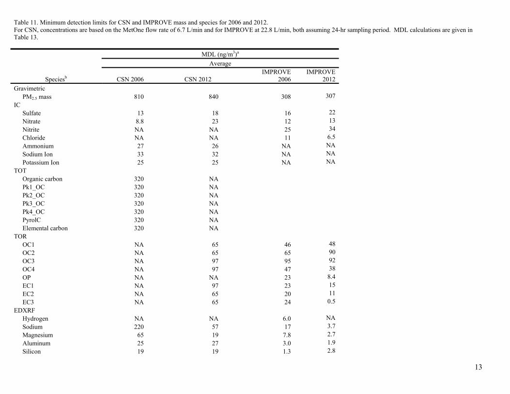
A summary of average MDL values (ng/m3) for the CSN SASS sampler for 2006 and

2012 is provided in Table 11 and results for all years since 2004 at TTN (2012a). Method

detection limits for OC, EC, and carbon fractions changed for CSN during this period, as shown

in Table 11, due to the change from the CSN OC/EC method to the IMPROVE OC/EC method.

IMPROVE: Individual MDL are provided with each concentration value in the

IMPROVE database. A concentration is determined to be significantly different from zero only if

it is greater than the MDL. For IC and TOR OC/EC analyses the MDL corresponds to twice the

standard deviation of the field blanks or backup QFF filters, respectively. For mass and light

absorption, the MDL corresponds to twice the analytical precision determined by laboratory

blanks (mass) or low-absorbing controls (light absorption). Prior to 2011, the MDL for each

element for PESA and EDXRF (the latter using the Cu and Mo anode XRF systems described

previously) was based on system blanks and specifically 3.29 times the square root of the

27

background counts under the region that would have been occupied if the element was present in

the sample (IMPROVE 1997). Beginning in 2011, the MDL for EDXRF (using the PANalytical

Epsilon 5) is determined as the 95th percentile of the intensity measured on a set of typically 50

to 100 field blanks (IMPROVE 2014a).

Lower MDL values reported in ambient concentrations (µg/m3) are observed for

IMPROVE relative to CSN because of the higher mass loading used in IMPROVE relative to the

MetOne SASS (Table 1; Hyslop and White 2008a). This relates to a factor of almost 6 potential

improvement in sensitivity (m3/cm2 of filter) often needed by IMPROVE due to the lower

ambient PM concentrations in pristine areas. Larger filter areas and lower flow rates were

employed in CSN to avoid filter clogging due to the higher PM concentrations observed in urban

locations. The effect of this theoretical advantage in sensitivity between the networks is an

important issue that will be investigated in a later paper. The ability to detect and quantify low

levels of elements in remote areas used as tracer species for certain sources (e.g., V, Se for oil

and coal combustion) could significantly impact the ability of receptor models to apportion

ambient PM to its sources (Flanagan et al. 2014).

Data Completeness

Completeness describes the amount of valid data obtained from a measurement system

compared to the amount that was expected to be obtained if all samples were collected

successfully. It is an important quality assurance indicator and provides a measure of data

validity. For example, when determining compliance for PM10, a minimum of 75 percent of the

scheduled PM10 samples per quarter are required for compliance calculations (Federal Register

2006, Part 50). Table 14 provides percent data completeness for major PM components for both

CSN and IMPROVE for two representative years, 2006 and 2012. Data completeness for both

networks was in the range of 90-100%.

Precision Based On Colocated Data

Whole-system precision estimates based on colocated sampling are obtained for both

networks according to the procedure described in the Federal Register (2006, Part 58, App. A,

section 4.3)..

28

Colocated CSN samplers have been operated at six STN sites since the beginning of the

program, accounting for between 3% and 5% of the entire network or roughly 12% of the STN

sites. The full network percentage has increased slightly as network reductions have taken place.

Colocated samplers at a given site are operated by the same operator and use filters prepared and

shipped at the same time, but shipped in separate containers. No effort is made to randomize the

filter pairs between laboratory instruments. Precision estimates for CSN based on colocated

sampling results are calculated annually and are summarized for the major species in the CSN

annual data summary reports (U.S. EPA 2012g). At each of the six colocated CSN sites, the

primary sampler operates on a 1-in-3 day schedule, while most of the colocated samplers operate

on a 1-in-6 day schedule.

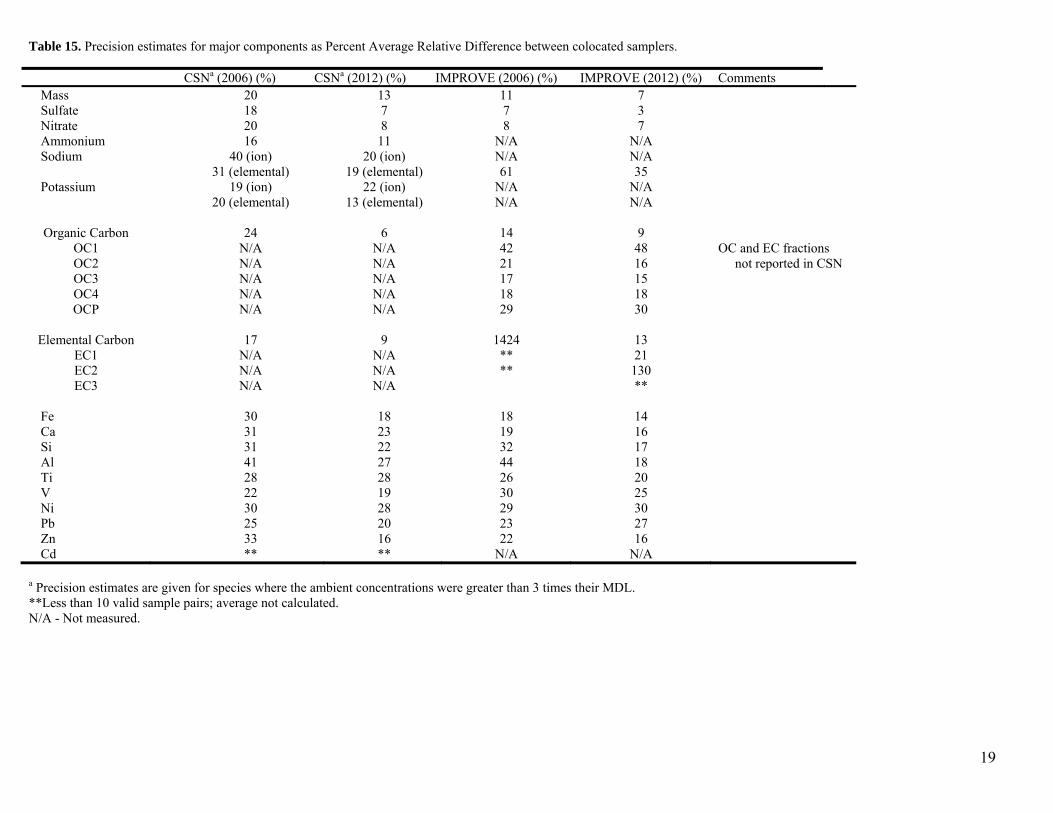
Precision results as percent average relative difference are presented in Table 15 for 2006

and 2012 for components that are typically 3 times above their MDL. Other elements are not

quantified so they are not included in the table. Precision results for CSN mass, ionic species (by

IC), and carbon components are around 20% ± 5%. Trace elements by EDXRF are mostly in the

range from 25% to 40%. Light elements analyzed by EDXRF such as sodium and aluminum

show relatively poor precision compared with heavier elements due to self-absorption as

described previously (see for example, Dzubay and Nelson 1975; Berry et al. 1969)

The IMPROVE sampler includes four filter holders per module (either A, B, C, or D; see

Figure 3) that have separate solenoid valves to allow for sequential sampling over multiple

sampling days. Prior to 2003, one of the four filter sets was used to obtain a colocated sample for

the specific filter type assigned to that module. Beginning in 2003, IMPROVE installed single

colocated modules (either A, B, C, or D) at different sites. Phoenix has all four modules

colocated. There are seven duplicate modules of each type (A, B, C, and D), which is equivalent

to having colocated samplers at 4% of the ~170 IMPROVE sites.

For major components, precision estimates in IMPROVE range from 3% for sulfate to

130% for the third elemental carbon fraction. Table 15 presents colocated precision estimates as

percent average relative difference determined from IMPROVE samples collected in 2006 and

2012. Colocated precision tends to improve with increasing data completeness, is typically better

29

when the analysis is performed on the whole filter instead of a fraction of the filter, and is better

for species that are predominantly in the fine size fractions (Hyslop and White 2008b).

CSN AND IMPROVE PROGRAM HISTORIES

Changes to network field sampling and analytical procedures can cause a step change in

reported data. Therefore, it is important to identify when these changes took place. Several

network changes took place in IMPROVE before 2000 and these are noted in the IMPROVE

newsletters (IMPROVE 2014b). Table 16 provides a brief history of the networks since 2000,

summarizes field and laboratory changes in both networks, and indicates the reason for the

change. Major changes are highlighted below with possible implications of that change to long-

term network results.

Between 2005 and 2006 CSN underwent a reduction in the number of monitoring

locations due to reduced funding. Most of the reductions occurred at SLAM sites and at locations

where PM concentrations no longer exceeded the PM NAAQS. However, the most significant

change to CSN began in early 2007 with replacement of the CSN carbon measurement approach

with the IMPROVE carbon measurement approach, albeit with minor exceptions as described

earlier (U.S. EPA 2007a-b; U.S. EPA 2009b; U.S. EPA 2012e). The replacement was completed

in October 2009 (U.S. EPA 2009b). Starting in 2008, CSN started transitioning to the

IMPROVE_A analysis method for carbon, which was completed by 2009. These changes were

implemented to obtain consistency between the two networks for carbon. A reduction in the

collection of network field blanks was applied to offset the increased cost of analyzing the

additional backup QFF used to estimate OC artifact.

It is anticipated that as sites were changed from the CSN OC/EC approach to the

IMPROVE approach a step change is likely to be observed, potentially with slightly lower OC

and higher EC; total carbon will likely change little (Chow et al. 2001, 2004; Schmid et al. 2001;

Conny et al. 2003; Watson et al. 2005; Cheng et al. 2011). This change also resulted in better

precision and lower MDL values for OC, EC, and OC fractions as seen in Table 11 in

comparison of 2006 to 2012. Since changing from the CSN to IMPROVE approach for OC and

EC took place over about 2.5 years, with a few sites at a time, the Carbon Conversion Site Lists

(U.S. EPA 2012e) will need to be reviewed on a site-by-site basis when examining long-term

30

trends for OC and EC during the period mid-2007 through near the end of 2009. However, the

consistency achieved between the networks for understanding regional impacts of carbon in

urban areas and vice versa was deemed sufficient reason for the change.

Several small changes have taken place since 2000, including switching to a smaller

shipping container and reducing the number of trace elements determined by EDXRF from 48 to

33 (see Table 11) since many of the elements removed were below their MDL. Both of these

were implemented to reduce cost but should have no long-term impact on the results. In 2009

CSN also adjusted the attenuation factor used for four low molecular weight elements. This

resulted in a small step change to the reported concentrations of these elements.

IMPROVE has had several changes since 2000, although most with only minor and

typically positive impacts on results. At the end of 2001, the analysis method for elements from

Na to Mn was changed from PIXE to EDXRF by Cu anode and at the end of 2002 EDXRF run

times were standardized at 1000 s. These changes resulted in improved and more consistent

detection limits for elements of interest. At the beginning of 2005 the carbon analysis instrument

was replaced with a new model resulting in a small change to the IMPROVE analysis approach

(IMPROVE_A) and details of this change can be found in Chow et al. (2007). In 2008 the

number of sites with QFF backup filters was increased from six to twelve providing better spatial

coverage and geographic diversity of the data used to correct for potential positive and negative

OC sampling artifacts. In 2011 the EDXRF was replaced with a new instrument (PANalytical

Epsilon 5); the list of elements reported remained unchanged. Also in 2011 the PESA analysis

for hydrogen was discontinued due to budget limitations. The hydrogen data from PESA were

used almost exclusively for quality control checks so eliminating the measurement had no effect

on most data analysis projects. Better precision and lower MDL values were realized for a

number of elements due to the switch to the PANalytical XRF systems. Improvements were

observed for sulfur and the soil-related elements required by the Regional Haze Rule as well as

improvements for the lighter elements such as sodium, aluminum, and silicon. There is

degradation of the precision and MDL values for some trace elements such as zinc and selenium.

31

SUMMARY AND CONCLUSIONS

This paper describes the CSN and IMPROVE networks in detail through 2012 with

minor updates through the beginning of 2014. It outlines the differences in the field and

laboratory approaches and summarizes the analytical parameters that affect data quality.

In general, the field and laboratory approaches used in the CSN and IMPROVE networks

are similar; yet there are many detailed and subtle differences in the sampling and analysis

methods employed, as well as shipping, blank/artifact estimation and correction approaches, and

estimation of uncertainties. These differences may be more or less important depending on the

application of the results and related policy objectives of the study using these data. Several

changes in measurement and analytical protocol also occurred since 2000. While some of these

changes may result in step changes in the long-term database they have been identified and in

general will have minimal impact on use of these data.

A recent assessment of the CSN network (Landis 2014) examined a range of parameters

that would suggest which sites to remove from the CSN network beginning in early 2015 due to

reduced budgets. The assessment considered, for example, the number of sites within a

geographic area, how PM correlated among those sites, and if the sites were within an attainment

area. Fifty-three sites were recommended for defunding. Other recommended network reductions

include eliminating the CSN mass measurement at the 119 sites beginning in July 2014 where

mass is measured by the FRM; reduce sampling frequency to 1 in 6 days at all but NCORE sites

(U.S. EPA 2005c; Scheffe et al. 2009) and STN sites; reduce carbon blanks from 10% – 5% and

eliminate carbon dynamic blanks currently at 5%. Implementation of recommendations is

schedule for early 2015 if approved and after all stakeholders have input. While not final, the

impact of these potential reductions will not be known for several years.

Future papers will directly compare results from colocated measurements at three urban

and three rural sites, each site having one of the three CSN samplers and an IMPROVE sampler

and examines if there are practical differences when using the same datasets in the same receptor

modeling application.

32

REFERENCES

Ashbaugh, L.L., and R.A. Eldred, 2004a. Loss of particle nitrate from Teflon sampling filters:

Effects on measured gravimetric mass in California and in the IMPROVE Network. J.

Air Waste Manage. Assoc. 54(1):93-104.

Ashbaugh, L.L., C.E. McDade, W.H. White, P. Wakabayashi, Collett, J.L. Jr., and Y. Xiao-Ying.

2004b. Efficiency of IMPROVE network denuders for removing nitric acid. In

Proceedings, Regional and Global Perspectives on Haze: Causes, Consequences and

Controversies, pp. 32-1 – 32-8. Air & Waste Management Association: Pittsburgh, PA.

Baker, W.C., and Pouchot, J.F. 1983. The measurement of gas flow, Part I. J. Air Waste Manage.

Assoc. 33:1, 66-72, DOI: 10.1080/00022470.1983.10465548.

Berry, P.F., T. Furuta, and J.R. Rhodes. 1969. Particle size effects in x-ray spectrometry. In

Advances in X-Ray Analysis, pp. 612-632. Ed. C.S. Barrett. New York, NY: Plenum

Press.

Bond, T.C., T.L. Anderson, and D.E. Campbell. 1999. Calibration and intercomparison of filter-

based measurements of visible light absorption by aerosols. Aerosol Sci. Technol.

30(6):582-600.

Bond T.C., and R.W. Bergstrom. 2006. Light absorption by carbonaceous particles: An

investigative review. Aerosol Sci. Technol. 40(1):27-67. DOI:

10.1080/02786820500421521.

Brook, J.R., E. Vega, J.G. Watson, J.M. Hales, and G.M. Hidy. 2004. Chapter 7: Receptor

Methods. Particulate Matter Science for Policy Makers - A NARSTO Assessment, Part 1,

pp. 235 -281. Cambridge, UK: Cambridge University Press:.

Cheng, Y., F.K. Duan, K.B. He, M. Zheng, Z.Y. Du, Y.L.Ma , J.H. Tan. 2011. Intercomparison

of thermal-optical methods for the determination of organic and elemental carbon:

Influences of aerosol composition and implications. Environ. Sci. Technol.,

45(23):10117-10123.

33

Chester. 2009. Standard Operating Procedure XR-002.04 Analysis of Elements in Air

Particulate~ by X-Ray Fluorescence (Kevex 770 & 772), US EPA 10 3.3. Tigard, OR.

http://www.epa.gov/ttn/amtic/files/ambient/pm25/spec/ChesterXR00204.pdf (accessed

May 29, 2014).

Chow, J.C. 1995. Measurement methods to determine compliance with ambient air quality

standards for suspended particles. J. Air Waste Manage. Assoc. 45(5):320-382.

http://www.tandfonline.com/doi/pdf/10.1080/10473289.1995.10467369 (accessed May

29, 2014).

Chow, J.C., J.G. Watson, L.C. Pritchett, W.R. Pierson, C.A. Frazier, and R.G. Purcell. 1993. The

DRI Thermal/Optical Reflectance carbon analysis system: Description, evaluation and

applications in U.S. air quality studies. Atmospheric Environment 27A(8):1185-1201.

Chow, J.C., J.G. Watson, D. Crow, D.H. Lowenthal, and T.M. Merrifield. 2001. Comparison of

IMPROVE and NIOSH carbon measurements. Aerosol Sci. Technol. 34(1):23-34.

Chow, J.C., J.G. Watson, L.W. A. Chen, W.P. Arnott, H. Moosmuller, and K.K. Fung. 2004.

Equivalence of elemental carbon by Thermal/Optical Reflectance and Transmittance with

different temperature protocols. Environ.l Sci. Technol. 38(16):4414-4422.

Chow, J.C., J.G. Watson, L.-W.A. Chen, G. Paredes-Miranda, M.-C.O. Chang, D.L. Trimble,

K.K. Fung, H. Zhang, and J.Z. Yu. 2005a. Refining temperature measures in

thermal/optical carbon analysis. Atmos. Chem. Phys. 5(4):2961-2972. http://www.atmos-

chem-phys.net/5/2961/2005/acp-5-2961-2005.pdf (accessed May 29, 2014)..

Chow, J.C., J.G. Watson, D.H. Lowenthal, and K.L. Magliano. 2005b. Loss of PM2.5 nitrate from

filter samples in Central California., J. Air Waste Manage. Assoc. 55:1158-1168.

Chow, J.C., J.G. Watson, L.-W.A. Chen, M.C.O. Chang, N.F. Robinson, D. Trimble, and S.

Kohl. 2007. The IMPROVE_A temperature protocol for Thermal/Optical Carbon

Analysis: Maintaining consistency with a long-term database. J. Air Waste Manage.

Assoc. 57(9):1014–1023.

34

Chow, J.C., P. Doraiswamy, J.G. Watson, L.-W.A. Chen, S.S.H. Ho, D.A. Sodeman. 2008.

Advances in integrated and continuous measurements for particle mass and chemical

composition. 58(2):141-163.

Chow, J.C., J.G. Watson, L.-W.A. Chen, J. Rice, and N.H. Frank. 2010. Quantification of PM2.5

organic carbon sampling artifacts in US networks. Atmos. Chem. Phys. 10:5223–5239

http://www.atmos-chem-phys.net/10/5223/2010/acp-10-5223-2010.pdf (accesssed May

29, 2014). .

Clark, M.S. 2002a. Nylon Filter Extraction Study July 30, 2002. Technical Memorandum to

James Homolya, U.S. EPA, Office of Air Quality Planning and Standards, Research

Triangle Park, NC. http://www.epa.gov/ttn/amtic/files/ambient/pm25/spec/nylfilstd.pdf

(accessed May 29, 2014).

Clark, M.S. 2002b. PM2.5 quartz filter experiments. Technical Memorandum to James Homolya,

U.S. EPA, Office of Air Quality Planning and Standards, Research Triangle Park, NC.

http://www.epa.gov/ttnamti1/files/ambient/pm25/spec/carboncsr.pdf (accessed May 29,

2014).

Clark, M.S. 2003. Nylon® Filter Extr action Study #2. Technical Memorandum to James

Homolya, U.S. EPA, Office of Air Quality Planning and Standards, Research Triangle

Park, NC. http://www.epa.gov/ttn/amtic/files/ambient/pm25/spec/nylstud2.pdf (accessed

May 29, 2014).

Conny, J.M., D.B. Klinedinst, S.A. Wight, and J.L.Paulsen. 2003. Optimizing thermal-optical

methods for measuring atmospheric elemental (black) carbon: A response surface study.

Aerosol Sci. Technol. 37:703-723. doi:10.1080/02786820390209662.

Coutant, B., and Stetzer, S. 2001. Evaluation of PM2.5 Speciation Sampler Performance and

Related Sample Collection and Stability Issues, Final Report. U.S. EPA, Office of Air

Quality Planning and Standards, Research Triangle Park, NC.

http://www.epa.gov/ttn/amtic/files/ambient/pm25/spec/minitrends.pdf (accessed May 29,

2014).

35

DRI. 2005. Standard Operating Procedure for the Determination of Carbon Fractions in

Particulate Matter Using the IMPROVE_A Heating Protocol on a Sunset Laboratory

Dual-Mode Analyzer. IMP_A Carbon Analysis of PM-SSL. Desert Research Institute,

Reno, NV.

http://www.epa.gov/ttn/amtic/files/ambient/pm25/spec/RTIIMPROVEACarbonAnalysisS

SLSOP.pdf (accessed May 29, 2014).

Dzubay, T.G., and R.O. Nelson. 1975. Self absorption corrections for x-ray fluorescence analysis

of aerosols. In Advances in X-Ray Analysis, Vol. 18, Eds. W.L. Pickles, C.S. Barrett, J.B.

Newkirk, and C.O. Rund, pp. 619-631. New York, NY, Plenum Publishing Corporation.

Eldred, R.A., T.A. Cahill, L.K. Wilkinson, P.J. Feeney, J.C. Chow, and W.C. Malm. 1990.

Measurement of fine particles and their chemical components in the NPS/IMPROVE

Networks. In Transactions, Visibility and Fine Particles, pp. 187-196. Ed. C.V. Mathai.

Pittsburgh, PA: Air Waste Management Association.

Federal Register. 1997. National Ambient Air Quality Standards for Particulate Matter: Final

Rule. 40 CFR Parts 50, 53, and 58, , July 18.

http://www.epa.gov/ttn/oarpg/t1/fr_notices/pmnaaqs.pdf (accessed May 29, 2014).

Federal Register. 1999. Part II, Environmental Protection Agency, 40 CFR Part 51, Regional

Haze Regulations, Final Rule, July 1.

http://www.epa.gov/ttn/oarpg/t1/fr_notices/rhfedreg.pdf (accessed May 29, 2014).

Federal Register. 2006. National Ambient Air Quality Standards for Particulate Matter: Final

Rule. 40 CFR Parts 50, 53, and 58, Volume 62 (138). Part 50: Part 53—Ambient Air

Monitoring Reference and Equivalent Methods. http://www.ecfr.gov/cgi-bin/text-

idx?SID=6786c9c05698e1df6a087fee4f1c0734&node=40:6.0.1.1.1&rgn=div5 (accessed

May 29, 2014).

Part 58—Ambient Air Quality Surveillance, http://www.ecfr.gov/cgi-bin/text-

idx?SID=6786c9c05698e1df6a087fee4f1c0734&node=40:6.0.1.1.6&rgn=div5 (accessed

May 29, 2014).

36

Federal Register. 2013. Ambient Air Monitoring Reference and Equivalent Methods, 40 CFR

Parts 53 - 59, Chapter 1, Subchapter C—Air Programs.

http://www.gpo.gov/fdsys/pkg/CFR-2013-title40-vol6/pdf/CFR-2013-title40-vol6.pdf

(accessed May 29, 2014).

Federal Register. 2014. Appendix B to Part 136—Definition and Procedure for the

Determination of the Method Detection Limit—Revision 1.11. 40 CFR Ch. I (7–1–12

Edition). file:///H:/Temp/Delete/CFR-2012-title40-vol24-part136-appB.pdf (accessed

May 29, 2014).

Fehsenfeld, F.C., D. Hastie, J.C. Chow, and P.A. Solomon. 2004. Particle and gas

measurements. Particulate Matter Science for Policy Makers, A NARSTO Assessment,

pp. 159-189. Eds. P.H. McMurry, M.F. Shepherd, J.S. Vickery. Cambridge, UK:

Cambridge University Press.

Fitz, D. 2002. Evaluation of Diffusion Denuder Coatings for Removing Acid Gases from Ambient

Air. U.S. Environmental Protection Agency, Office of Air Quality Planning and

Standards, Research Triangle Park, NC.

http://www.epa.gov/ttnamti1/files/ambient/pm25/spec/denudr.pdf (accessed May 29,

2014).

Flocchini, R., L. Ashbaugh, R. Eldred, P. Feeney, S. Ixquiac, P. Beveridge. 2002. Quality

Assurance Guidance Document Revision 0.0. IMPROVE: Interagency Monitoring of

Protected Visual Environments, Quality Assurance Project Plan, OAQPS Category 1

QAPP. UC Davis, Davis, CA.

http://vista.cira.colostate.edu/improve/publications/QA_QC/IMPROVE_QAPP_R0.pdf

(accessed May 29, 2014).

Flanagan, J., L. Michael, R.K.M. Jayanty, K. Baumann, and P.A. Solomon. 2014. National

PM2.5 Monitoring Networks in the United States—CSN/STN and IMPROVE:

Intercomparison of PMF receptor modeling results using data from colocated IMPROVE

and CSN PM2.5 chemical speciation samplers. In preparation.

37

Gego, E. L., P.S. Porter, J.S. Irwin, C. Hogrefe, and S.T. Rao. 2005. Assessing the comparability

of ammonium, nitrate and sulfate concentrations measured by three air quality monitoring

networks. Pure Appl. Geophys. 162:1919–1939.

Gutknecht, W.F., J.A. O'Rourke, J.B. Flanagan, W.C. Eaton, M.R. Peterson, and L.C. Greene.

2001. Research to investigate the source(s) of high field blanks for Teflon® PM2.5 filters.

Report Number RTI/07565/019-01FR, EPA Contract No. 68-D-99-0013, prepared by

Research Triangle Institute, Center for Environ. Measurement & Quality Assurance,

Research Triangle Park, NC for U.S. EPA, Research Triangle Park, NC.

Gutknecht, W.F., J.B. Flanagan, and A. McWilliams. 2006. Harmonization of interlaboratory X-

ray fluorescence measurement uncertainties. Research Triangle Institute, Research

Triangle Park, NC. http://www.epa.gov/ttn/amtic/files/ambient/pm25/spec/xrfdet.pdf

(accessed May 29, 2014).

Gutknecht, W., J. Flanagan, A. McWilliams, R.K.M. Jayanty, R. Kellogg, J. Rice, P. Duda, and

R.H. Sarver. 2010. Harmonization of uncertainties of X-ray fluorescence data for PM2.5

air filter analysis. J. Air Waste Manage. Assoc. 60(2):184-194.

Harrison, R.M., and J. Yin. 2000. Particulate matter in the atmosphere: Which particle properties

are important for its effects on health? Sci. Total Environ. 249(1-3):85-101.

Hering, S.V., D.R. Lawson, P.A. Solomon, et al. 1988. The Nitric Acid Shootout: Field

comparison of measurement methods. Atmos. Environ. 22(8):1519-1539.

Hering, S.V., and G.R. Cass. 1999. The magnitude of bias in the measurement of PM2.5 arising

from volatilization of particulate nitrate from Teflon filters., J. Air Waste Manage. Assoc.

49:725-733.

Hering, S., P.M. Fine, C. Sioutas, P.A. Jaques, J.L. Ambs, O. Hogrefe, and K.L. Demerjian.

2004. Field assessment of the dynamics of particulate nitrate vaporization using

differential TEOM and automated nitrate monitors Atmos. Environ. 38:5183-5192.

Hinds, W.C. 1999. Aerosol Technology. Properties, Behavor, and Measurement of Airborne

Particles. New York, NY: John Wiley & Sons.

38

Hopke, P.K. 1991. Receptor Modeling for Air Quality Management, Hopke,P.K., Ed.,

Amsterdam: Elsevier.

Hopke, P.K. 2003. Recent developments in receptor modeling. J.Chemometrics 17(5):255-265.

Hyslop, N.P., and W.H. White. 2008a. An empirical approach to estimating detection limits

using colocated data. Environ Sci Technol 42(14):5235-5240.

Hyslop, N.P.. and W.H. White. 2008b. An evaluation of interagency monitoring of protected

visual environments (IMPROVE) colocated precision and uncertainty estimates. Atmos.

Environ. 42(11):2691-2705.

IMPROVE. 1997. SOP 301, IMPROVE Standard Operating Procedures for X-Ray Fluorescence

Analysis, 2/4/97. Colorado State University, Boulder,

CO.http://vista.cira.colostate.edu/improve/Publications/SOPs/ucdavis_sops/sop301.pdf

(accessed May 29, 2014).

IMPROVE. 2002. IMPROVE: Interagency Monitoring of Protected Visual Environments

Quality Assurance Project Plan OAQPS Category 1 QAPP. Colorado State University,

Boulder, CO.

http://vista.cira.colostate.edu/improve/Publications/QA_QC/IMPROVE_QAPP_R0.pdf

(accessed May 28, 2014).

IMPROVE. 2005. Standard Operating Procedures for National Park Service Filter Preparation,

Extraction, and Anion Analysis. Colorado State University, Boulder, CO.

http://vista.cira.colostate.edu/improve/Publications/SOPs/RTI_SOPs/RTI_IonSOP10260

5.pdf (accessed May 29, 2014).

IMPROVE. 2006. Report IV, November. Colorado State University, Boulder, CO.

http://vista.cira.colostate.edu/improve/Publications/Reports/2006/2006.htm (accessed

May 29, 2014).

IMPROVE. 2012a. Interagency Monitoring of Protected Visual Environments. Colorado State

University, Boulder, CO. http://vista.cira.colostate.edu/improve/ (accessed May 29,

2014).

39

IMPROVE. 2012b. IMPROVE Standard Operating Protocols. Colorado State University,

Boulder, CO. http://vista.cira.colostate.edu/improve/Publications/IMPROVE_SOPs.htm

(accessed May 29, 2014).

IMPROVE. 2012c. SOP 201, Sampler Maintenance by Site Operators. Colorado State

University, Boulder, CO.

http://vista.cira.colostate.edu/improve/Publications/SOPs/ucdsop.asp (accessed May 29,

2014).

IMPROVE. 2012d. SOP 251, Sample Handling. Colorado State University, Boulder, CO.

http://vista.cira.colostate.edu/improve/Publications/SOPs/UCDavis_SOPs/SOP251_Samp

le_Handling_2013.pdf (accessed May 29, 2014).

IMPROVE. 2012e. Quality assurance for the IMPROVE network. Colorado State University,

Boulder, CO. http://vista.cira.colostate.edu/improve/Data/QA_QC/qa_qc_Branch.htm

(accessed May 29, 2014).

IMPROVE. 2012f. SOP 326, PIXE and PESA Analysis. Colorado State University, Boulder, CO.

http://vista.cira.colostate.edu/improve/Publications/SOPs/ucdsop.asp (accessed May 29,

2014).

IMPROVE. 2012g. IMPROVE Data advisories. Colorado State University, Boulder, CO.

http://vista.cira.colostate.edu/improve/Data/QA_QC/Advisory.htm (accessed May 29,

2014).

IMPROVE. 2014a. IMPROVE Standard Operating Procedure for the X-Ray Fluorescence

Analysis of Aerosol Deposits on PTFE Filters (with PANalytical Epsilon 5) SOP 301,

SOP 301, Version 2, January 17, 2014. Colorado State University, Boulder, CO.

http://vista.cira.colostate.edu/improve/Publications/SOPs/ucdavis_sops/sop301_XRF_20

14.pdf (accessed May 29, 2014).

IMPROVE. 2014b. IMPROVE quarterly newsletters. Colorado State University, Boulder, CO.

http://vista.cira.colostate.edu/improve/Publications/news_letters.htm (accessed May 29,

2014).

40

Iyer, H., P. Patterson, and W.C. Malm. 2000. Sampling duration calculations. J. Air Waste

Manage. Assoc. 50(5):888-893.

John, W., and G. Reischl 1980. A cyclone for size-selective sampling of ambient air. J. Air Poll.

Control Assoc., 30(8):872-876.

Kampa, M., and E. Castanas. 2008. Human health effects of air pollution. Environ. Pollut.

151(2):362-367. doi: 10.1016/j.envpol.2007.06.012.

Kenny, L.C., and R.A. Gussman. 2000. A direct approach to the design of cyclones for aerosol-

monitoring applications. J. Aerosol Sci. 31(12):1407-1420.

Kenny, L.C., and R.A. Gussman, M.B. Meyer. 2000. Development of a sharp-cut cyclone for

ambient aerosol monitoring applications. Aerosol Sci. Technol. 32(4):338-358.

Kenny, L., G. Beaumont, A. Gudmundsson, A. Thorpe, and W. Koch. 2005. Aspiration and

sampling efficiencies of the TSP and louvered particulate matter inlets. J. Environ.

Monitoring 7(5):481-487

Kim, B.M., J. Cassmassi, H. Hogo, and M.D. Zeldin. 2001. Positive organic carbon artifacts on

filter medium during PM2.5 sampling in the South Coast Air Basin. Aerosol Sci. Technol.

34(1):35-41.

Kim, E., P.K. Hopke,and Y. Qin. 2005. Estimation of organic carbon blank values and error

structures of the speciation trends network data for source apportionment. J. Air Waste

Manage. Assoc. 55(8):1190-1199.

Koutrakis, P. 1998. Recommendations of the Expert Panel On the EPA Speciation Network.

Prepared for Office of Air and Radiation, OAQPS, Research Triangle Park, NC.

http://www.epa.gov/ttnamti1/files/ambient/pm25/spec/speciate.pdf (accessed May 29,

2014).

Koutrakis, P. 1999. Recommendations of the Expert Panel on the EPA Speciation Network (Draft

7/12/99). Research Triangle Institute, Research Triangle Park, NC.

41

http://www.epa.gov/ttnamti1/files/ambient/pm25/spec/lvpanel.pdf (accessed May 29,

2014).

Landis, B. 2014. CSN network assessment. ORD Sponsored Webinar, May 1, 2014. Research

Triangle Park, NC. http://epa.gov/ncer/events/calendar/2014/may01/presentation.pdf.

CSN assessment - Decision matrix for 53 low value sites recommended for defunding.

http://epa.gov/ncer/events/calendar/2014/may01/defund-list.pdf (accessed May 29, 2014).

Lewtas, J., Y. Pang, D. Booth, S. Reimer, D.J. Eatough, L.A. Gundel. 2001. Comparison of

sampling methods for semi-volatile organic carbon associated with PM2.5. Aerosol Sci.

Technol. 34(1):9-22.

Maimone, F., B.J. Turpin, P. Solomon, Q. Meng, A.L. Robinson, R. Subramanian, and A.

Polidori. 2011. Correction methods for organic carbon artifacts when using quartz-fiber

filters in large particulate matter monitoring networks: The regression method and other

options. J. Air Waste Manage. Assoc. 61(6):696-710.

Malm, W.C., B.A. Schichtel, M.L. and Pitchford. 2011. Uncertainties in PM2.5 gravimetric and

speciation measurements and what we can learn from them. J. Air Waste Manage. Assoc.

61(11):1131-1149.

McCarthy, G. 2013. Initial area designations for the 2012 Revised Primary Annual Fine Particle

National Ambient Air Quality Standard. U.S. Environmental Protection Agency,

Washington DC.

http://www.epa.gov/pmdesignations/2012standards/docs/april2013guidance.pdf

(accessed May 29, 2014).

McClellan, R., B. Jessiman, P. McMurry, M. Shepherd, and J. Vickery. 2004. Health context for

management of particulate matter. In Particulate Matter Science for Policy Makers - A

NARSTO Assessment, pp. 69-101. Eds. P.H. McMurry, M.F. Shepherd, J.S. Vickery.

Cambridge, UK: Cambridge University Press:.

Charles E. McDade, C.E.; Dillner, A.M., and Indresand, H. 2009 Particulate matter sample

deposit geometry and effective filter face velocities, J. Air Waste Manage. Assoc.

42

59(9):1045-1048. DOI: 10.3155/1047-3289.59.9.1045.

http://www.tandfonline.com/doi/pdf/10.3155/1047-3289.59.9.1045 (accessed May 30,

2014)

McDow, S.R., and Huntzicker, J.J. 1990. Vapor adsorption artifact in the sampling of organic

aerosol: face velocity effects. Atmos. Environ. 24:2563-2571.

Pang, Y., N.L. Eatough, J. Wilson, and D.J. Eatough. 2002. Effect of semi-volatile material on

PM2.5 measurement by the PM2.5 Federal Reference Method sampler at Bakersfield,

California. Aerosol Sci. Technol. 36:289-299.

Peters, A.J., D.A. Lane, L.A. Gundel, G.L. Northcott, and K.C. Jones. 2000. A comparison of

high volume and diffusion denuder samplers for measuring semivolatile organic

compounds in the atmosphere. Environ. Sci. Technol. 34:5001-5006.

Peters, T.M., R.A. Gussman, L.C. Kenny, and R.W. Vanderpool. 2001. Evaluation of PM2.5 size

selectors used in speciation samplers. Aerosol Sci. Techno. 34(5):422-429.

Peterson, M.R., J. Smiley, S. Taylor, Jr., R.L. Hines, and M.H. Richards 2007. Effects of quartz

filter type on sampling and organic carbon/elemental carbon analysis of PM2.5. RTI

International, Research Triangle Park, NC.

http://www.epa.gov/ttn/amtic/files/ambient/pm25/spec/20070103quartzfiltercomparison.

pdf (accessed May 29, 2014).

Peterson, M.R., Richards, M.H. 2002. Thermal-optical-transmittance analysis for organic,

elemental, carbonate, total carbon, and OCX2 in PM2.5 by the EPA/NIOSH method. In

Proceedings, Symposium on Air Quality Measurement Methods and Technology-2002,

pp. 83-1 – 83-19. Eds. E.D. Winegar, R.J. Tropp. Pittsburgh, PA: Air & Waste

Management Association.

RTI. 2008. Standard Operating Procedure for PM2.5 Gravimetric Analysis, Revision 7. RTI

International, Research Triangle Park, NC.

http://www.epa.gov/ttn/amtic/files/ambient/pm25/spec/RTIGravMassSOPFINAL.pdf

43

(accessed May 29, 2014). Updates may be available at

http://www.epa.gov/ttn/amtic/specsop.html (accessed May 29, 2014).

RTI. 2009a. Standard Operating Procedures for Coating Aluminum Honeycomb Denuders With

Magnesium Oxide. RTI International, Research Triangle Park, NC. Updates may be

available at http://www.epa.gov/ttn/amtic/specsop.html (accessed May 29, 2014).

RTI. 2009b. Standard Operating Procedure for Cleaning Nylon Filters Used for Collection of

PM2.5 Material. RTI International, Research Triangle Park, NC.

http://www.epa.gov/ttn/amtic/files/ambient/pm25/spec/pm25nyloncleaningsop.pdf (last

accessed My 29, 2014). Updates may be available at

http://www.epa.gov/ttn/amtic/specsop.html (accessed May 29, 2014).

RTI. 2009c. Standard Operating Procedure for PM2.5 Cation Analysis. RTI International,

Research Triangle Park, NC.

http://www.epa.gov/ttn/amtic/files/ambient/pm25/spec/pm25cationsop.pdf (accessed

May 29, 2014). Updates may be available at http://www.epa.gov/ttn/amtic/specsop.html

(accessed May 29, 2014).

RTI. 2009d. Standard Operating Procedure for PM2.5 Anion Analysis. RTI International,

Research Triangle Park, NC.

http://www.epa.gov/ttn/amtic/files/ambient/pm25/spec/pm25anionsop.pdf (accessed May

29, 2014). Updates may be available at http://www.epa.gov/ttn/amtic/specsop.html

(accessed May 29, 2014).

RTI. 2009e. Standard Operating Procedure for the Determination of Organic, Elemental, and

Total Carbon in Particulate Matter Using a Thermal/Optical Transmittance Carbon

Analyzer. RTI International, Research Triangle Park, NC.

.http://www.epa.gov/ttn/amtic/files/ambient/pm25/spec/RTIOCECSOP.pdf (last accessed

May 29, 2014). Updates may be available at http://www.epa.gov/ttn/amtic/specsop.html

(accessed May 29, 2014).

RTI. 2009f. Standard Operating Procedure for the X-ray Fluorescence Analysis of PM2.5

Deposits on Teflon Filters.

44

http://www.epa.gov/ttn/amtic/files/ambient/pm25/spec/pmxrfsop.pdf (accessed May 29,

2014). Updates may be available at http://www.epa.gov/ttn/amtic/specsop.html (accessed

May 29, 2014). RTI International, Research Triangle Park.

RTI. 2011. Standard Operating Procedure for Procurement and Acceptance Testing of Teflon,

Nylon, and Quartz Filters. RTI International, Research Triangle Park, NC.

http://www.epa.gov/ttn/amtic/files/ambient/pm25/spec/RTIFilterProcurementSOPFINAL

.pdf (accessed May 29, 2014). Updates may be available at

http://www.epa.gov/ttn/amtic/specsop.html (accessed May 29, 2014).

RTI. 2013. Chemical Speciation - Field Standard Operating Procedures. RTI International,

Research Triangle Park, NC. http://www.epa.gov/ttn/amtic/spectraining.html (accessed

May 29, 2014). Updates may be available.

Schauer, J.J., W.F. Rogge, M.A. Mazurek, L.M. Hildemann, G.R. Cass, and B.R.T. Simoneit.

1996. Source apportionment of airborne particulate matter using organic compounds as

tracers. Atmos. Environ. 30(22):3837-3855.

Scheffe R.D., P.A. Solomon, R. Husar, et al. 2009. The National Ambient Air Monitoring

Strategy: Rethinking the role of national networks. J. Air Waste Manage. Assoc. 59:579-

590.

Schmid, H.P., L. Laskus, H.J. Abraham, U. Baltensperger, V.M. H. Lavanchy, M. Bizjak, P.

Burba, H. Cachier, D. Crow, J.C. Chow, T. Gnauk, A. Even, H.M. ten Brink, K.P.

Giesen, R. Hitzenberger, C. Hueglin, W. Maenhaut, C.A. Pio, J. Puttock, J.P. Putaud, D.

Toom-Sauntry, and H. Puxbaum. 2001. Results of the "Carbon Conference" international

aerosol carbon round robin test: Stage 1. Atmos. Environ. 35(12):2111-2121.

Seinfeld, J.H., and S.N. Pandis. 1998. Atmospheric Chemistry and Physics from Air Pollution to

Climate Change. New York, NY: John Wiley and Sons.

Smiley, J. 2013. Experimental Inter-comparison of Speciation Laboratories – Study#8. Research

Triangle Park, NC, Technical Memorandum to Dennis Crumpler, June 26, 2013. U.S.

EPA, Office of Air Quality Planning and Standards.

45

http://www.epa.gov/ttn/amtic/files/ambient/pm25/qa/MultilabSpeciationPT2012.pdf

(accessed May 29, 2014) Previous reports are available at

http://www.epa.gov/ttn/amtic/pmspec.html (accessed May 29, 2014)..

Solomon, P.A., L. Salmon, T. Fall, and G.R. Cass. 1992. The spatial and temporal distribution of

atmospheric nitric acid and particulate nitrate concentrations in Los Angeles. Environ.

Sci. Technol. 26(8):1594-1601.

Solomon, P.A., W. Mitchell, D. Gemmill, M.P. Tolocka, G. Norris, R. Wiener, S. Eberly, J.

Rice, J. Homolya, R. Scheffe, R. Vanderpool, R. Murdoch, S. Natarajan, and E. Hardison.

2000. Evaluation of PM2.5 chemical speciation samplers for use in the U.S. EPA National

PM2.5 Chemical Speciation Network. Office of Air Quality Planning and Standards,

Research Triangle Park, NC.

http://www.epa.gov/ttnamti1/files/ambient/pm25/spec/fourcty.pdf (accessed May 29,

2014).

Solomon, P.A., M.P. Tolocka, G. Norris, M. Landis. 2001. Chemical analysis methods for

atmospheric aerosol components. Aerosol Measurement: Principles, Techniques, and

Application, pp. 261-293. Ed. P. Baron and K. Willeke. New York, NY:John Wiley &

Sons, Inc.

Solomon, P.A., K. Baumann, E. Edgerton, R. Tanner, D. Eatough, W. Modey, H. Maring, D.

Savoie, S. Natarajan, M.B. Meyer, and G. Norris. 2003. Comparison of integrated

samplers for mass and composition during the 1999 Atlanta Supersites project. J.

Geophys. Re. 108(D7):8423. doi: 10.1029/2001JD001218.

Solomon, P.A., and P.K. Hopke. 2008. Introduction: special issue supporting key scientific and

policy- and health-relevant findings from EPA's Particulate Matter Supersites Program

and related studies: An integration and synthesis of results. Eds. P.A. Solomon, and P.K.

Hopke. J. Air Waste Manage. Assoc. 58(2):137-139.

Solomon, P.A., P.K. Hopke, J. Froines, and R. Scheffe. 2008. Key scientific and policy- and

health-relevant findings from EPA’s Particulate Matter Supersites Program and related

46

studies: An integration and synthesis of results. J. Air Waste Manage. Assoc. 58(13):S1-

S92.

Solomon, P.A., M. Costantini, T.J. Grahame, M.E. Gerlofs-Nijland, F. Cassee, A.G. Russell, J.R.

Brook, P.K. Hopke, G. Hidy, R.F. Phalen, P. Saldiva, S. Ebelt Sarnat, J.R. Balmes, I.B.

Tager, H. Özkaynak, S. Vedal, S.S.G. Wierman, and D.L. Costa. 2012. Air Pollution and

Health: Bridging the Gap from Sources to Health Outcomes: Conference summary. Air

Quality, Atmos. and Health 5(1):9-62. DOI: 10.1007/s11869-011-0161-4.

Subramanian, R., A.Y. Khlystov, J.C. Cabada, and A.L. Robinson. 2004. Positive and negative

artifacts in particulate organic carbon measurements with denuded and undenuded

sampler configurations. Aerosol Sc. Technol. 38(Suppl 1):27-48.

TTN. 2012a. Chemical Speciation - Data Management and Reporting. Technology Transfer

Network Ambient Monitoring Technology, AMTIC. US EPA, OAQPS, Research

Triangle Park, NC. http://www.epa.gov/ttn/amtic/specdat.html (accessed May 29, 2014).

TTN. 2012b. Chemical Speciation - Special Studies. Technology Transfer Network Ambient

Monitoring Technology, AMTIC, US EPA, OAQPS, Research Triangle Park, NC.

http://www.epa.gov/ttn/amtic/specstud.html (accessed May 29, 2014).

Tolocka, M.P., P.A. Solomon, W. Mitchell, G.A. Norris, D. B. Gemmill, R.W. Wiener, R.W.

Vanderpool, J.B. Homolya, and J. Rice. 2001. East versus west in the U.S: Chemical

characteristics of PM2.5 during the winter of 1999. Aerosol Sci. Technol. 34(1):88-96.

Turpin, B.J., S.V. Hering, and J.J. Huntzicker. 1994. Investigation of organic aerosol sampling

artifacts in the Los Angeles Basin, Atmos. Environ. 28:3061-3071.

Turpin, B.J., P. Saxena, and E. Andrews. 2000. Measuring and simulating particulate organics in

the atmosphere: Problems and prospects. Atmospheric Environment 34(18): 2983-3013.

U.S. EPA. 1998. Quality Assurance Guidance Document 2.12 Monitoring in PM2.5 Ambient Air

Using Designated Reference or Class I Equivalent Methods. U.S. Environmental

Protection Agency, Office of Air Quality Planning and Standards, Research Triangle

47

Park, NC. http://www.epa.gov/ttn/amtic/files/ambient/pm25/qa/m212covd.pdf (accessed

May 29, 2014).

U.S. EPA. 1999a. Particulate Matter (PM2.5) Speciation Guidance Final Draft, October 7, 1999.

U.S. Environmental Protection Agency, Monitoring and Quality Assurance Group,

Emissions, Monitoring, and Analysis Division, Office of Air Quality Planning and

Standards, Research Triangle Park, NC.

http://www.epa.gov/ttn/amtic/files/ambient/pm25/spec/specfinl.pdf (accessed May 29,

2014).

U.S. EPA. 1999b. Data Quality Objectives for the Trends Component of the PM2.5 Speciation

Network. U.S. Environmental Protection Agency, Office of Air Quality Planning and

Standards, Research Triangle Park, NC.

http://www.epa.gov/ttn/amtic/files/ambient/pm25/spec/dqo3.pdf (accessed May 29,

2014).

U.S. EPA. 1999c. Compendium of Methods for the Determination of Inorganic Compounds in

Ambient Air Compendium Method IO-3.3 Determination of Metals in Ambient

Particulate Matter Using X-Ray Fluorescence (XRF) Spectroscopy. U.S. Environmental

Protection Agency, Office of Air Quality Planning and Standards, Research Triangle

Park, NC. http://www.epa.gov/ttnamti1/files/ambient/inorganic/mthd-3-3.pdf (accessed

May 29, 2014).

U.S. EPA. 2000. Quality Assurance Guidance Document, Final Quality Assurance Project Plan:

PM2.5 Speciation Trends Network Field Sampling. U.S. Environmental Protection

Agency, Office of Air Quality Planning and Standards, Research Triangle Park, NC.

http://www.epa.gov/ttn/amtic/files/ambient/pm25/spec/1025sqap.pdf (accessed May 29,

2014).

U.S. EPA. 2005a. PM2.5 Speciation Network Newsletter, Issue 4, October. U.S. Environmental

Protection Agency, Office of Air Quality Planning and Standards, Research Triangle

Park, NC. http://www.epa.gov/ttn/amtic/files/ambient/pm25/spec/spnews4.pdf (accessed

May 29, 2014).

48

U.S. EPA. 2005b. PM2.5 Speciation Network Newsletter, Issue 2, January. U.S. Environmental

Protection Agency, Office of Air Quality Planning and Standards, Research Triangle

Park, NC. http://www.epa.gov/ttn/amtic/files/ambient/pm25/spec/spnews2.pdf (accessed

May 29, 2014).

U.S. EPA. 2005c. DRAFT, National Ambient Air Monitoring Strategy. U.S. Environmental

Protection Agency, Office of Air Quality Planning and Standards, Research Triangle

Park, NC. http://www.epa.gov/ttn/amtic/files/ambient/monitorstrat/naamstrat2005.pdf

(accessed May 29, 2014).

U.S. EPA. 2006. PM2.5 Speciation Network Newsletter, Issue 5, April. U.S. Environmental

Protection Agency, Office of Air Quality Planning and Standards, Research Triangle

Park, NC. http://www.epa.gov/ttn/amtic/files/ambient/pm25/spec/spnews5.pdf (accessed

May 29, 2014).

U.S. EPA. 2007a. EPA PM2.5 Chemical Speciation Network Carbon Sampler Replacement

Program: Phase I. U.S. Environmental Protection Agency, Office of Air Quality

Planning and Standards, Research Triangle Park, NC.

http://www.epa.gov/ttn/amtic/files/ambient/pm25/spec/EPA_Carbon_report%20ARS%20

JRICE%2010-10-07.pdf (accessed May 29, 2014).

U.S. EPA. 2007b. URG 3000N phase I carbon implementation report, August 2007. Prepared by

U.S. Environmental Protection Agency, Research Triangle Park, NC, U.S. Environmental

Protection Agency, Research Triangle Park, NC,

http://www.epa.gov/ttn/amtic/files/ambient/pm25/spec/EPA_Carbon_report%20ARS%20

JRICE%2010-10-07.pdf (accessed May 29, 2014).

U.S. EPA. 2007c. Field/trip blank collection for carbon in the PM2.5 Chemical Speciation

Network (CSN) Changes with the new URG3000N carbon measurement system, Note to

URG3000N Phase 1 Implementation Group1, July 18, 2007. U.S. Environmental

Protection Agency, Office of Air Quality Planning and Standards, Research Triangle

Park, NC. http://www.epa.gov/ttnamti1/files/ambient/pm25/spec/blank-Schedule.pdf

(accessed May 29, 2014).

49

U.S. EPA. 2009a. Integrated science assessment for particulate matter (EPA/ 600/R-08/139F).

U.S. Environmental Protection Agency, Office of Research and Development, Research

Triangle Park, NC. http://cfpub.epa.gov/ncea/cfm/recordisplay.cfm?deid=216546

(accessed May 29, 2014).

U.S. EPA. 2009b. URG3000N phase II carbon implementation report. Prepared by U.S.

Environmental Protection Agency, Research Triangle Park, NC, U.S. Environmental

Protection Agency, Research Triangle Park, NC,

http://www.epa.gov/ttn/amtic/files/ambient/pm25/spec/URG3000NPhaseIIReportFinal.p

df (accessed May 29, 2014).

U.S. EPA. 2011. PM 2.5 Speciation - Lab Audit Reports and Assessments. U.S. EPA, National

Air and Radiation Environmental Laboratory, Montgomery, AL.

http://www.epa.gov/ttn/amtic/pmspec.html (accessed May 29, 2014).

U.S. EPA. 2012a. Technology Transfer Network (TTN), Air Quality System (AQS). U.S.

Environmental Protection Agency, Office of Air Quality Planning and Standards,

Research Triangle Park, NC. http://www.epa.gov/ttn/airs/airsaqs/ (accessed May 29,

2014).

U.S. EPA. 2012b. Technology Transfer NetworkAmbient Monitoring Technology Information

Center,Chemical Speciation. U.S. Environmental Protection Agency, Office of Air

Quality Planning and Standards, Research Triangle Park, NC.

http://www.epa.gov/ttnamti1/speciepg.html (accessed May 29, 2014).

U.S. EPA. 2012c. CSN and IMPROVE Air Sampler Photographs and Diagrams. U.S.

Environmental Protection Agency, Office of Air Quality Planning and Standards,

Research Triangle Park, NC.

http://www.epa.gov/ttn/amtic/files/ambient/pm25/spec/pm25pict.pdf (accessed May 29,

2014).

U.S. EPA. 2012d. Quality Assurance Guidance Document Quality Assurance Project Plan:

PM2.5 Chemical Speciation Sampling at Trends, NCore, Supplemental and Tribal Sites

(An Update to the PM2.5 Speciation Trends Network Field Sampling QAPP, December

50

2000), EPA EPA-454/B-12-003. U.S. Environmental Protection Agency, Office of Air

Quality Planning and Standards, Research Triangle Park, NC.

http://www.epa.gov/ttn/amtic/files/ambient/pm25/spec/CSN_QAPP_v120_05-2012.pdf

(accessed May 29, 2014)..

U.S. EPA. 2012e. Chemical Speciation - URG3000N Carbon Implementation. . U.S.

Environmental Protection Agency, Office of Air Quality Planning and Standards,

Research Triangle Park, NC. http://www.epa.gov/ttn/amtic/specurg3000.html (accessed

May 29, 2014).. U.S. EPA. 2012f. Quality Assurance Project Plan, Chemical Speciation

of PM2.5 Filter Samples. U.S. Environmental Protection Agency, Office of Air Quality

Planning and Standards, Research Triangle Park, NC. Rpt. RTI/0212053/01QA, May

2012. http://www.epa.gov/ttn/amtic/files/ambient/pm25/spec/qapp.pdf (accessed May 29,

2014). , last asccessed 4-24-24.

U.S. EPA 2013. Master CSN Site List Including Trends 2013. U.S. Environmental Protection

Agency, Office of Air Quality Planning and Standards, Research Triangle Park,

NC.http://www.epa.gov/ttnamti1/files/ambient/pm25/spec/MasterCSNListforAMTIC050

313.xlsx (accessed May 29, 2014).

Watson, J.G., J.C. Chow, and L.-W.A. Chen. 2005. Summary of organic and elemental

carbon/black carbon analysis methods and intercomparisons. Aerosol Air Quality Res.

5(1):65-102. http://aaqr.org/VOL5_No1_June2005/6_AAQR-05-06-OA-0006_65-

102.pdf (accessed May 29, 2014).

Watson, J.G., L.W. Chen, J.C. Chow, P. Doraiswamy, and D.H. Lowenthal. 2008. Source

apportionment: findings from the U.S. Supersites Program. J. Air Waste Manage. Assoc.

58(2):265-288.

Watson, J.G., J.C. Chow, L.W. Chen, N.H. Frank. 2009. Methods to assess carbonaceous aerosol

sampling artifacts for IMPROVE and other long-term networks. J. Air Waste Manage.

Assoc. 59:898-911.

51

Watson, J.G., and J.C. Chow. 2011. Ambient aerosol sampling. In Aerosol Measurement:

Principles, Techniques and Applications, Third Edition, pp. 591-614Eds. P. Kulkarni,

P.A. Baron, and K. Willeke. Hoboken, NJ: John Wiley & Sons, Inc..

White, W.H., L.L. Ashbaugh, N.P. Hyslop, and C.E. McDade. 2005. Estimating measurement

uncertainty in an ambient sulfate trend. Atmos. Environ. 39(36):6857-6867.

Yu, X.Y., T. Lee, B. Ayres, S.M. Kreidenweis, W. Malm, and J.L. Collett. 2006. Loss of fine

particle ammonium from denuded nylon filters. Atmos. Environ. 40(25):4797-4807.

Zhao, W.X., P.K. Hopke, G. Norris, R. Williams, and P. Paatero. 2006. Source apportionment

and analysis on ambient and personal exposure samples with a combined receptor model

and an adaptive blank estimation strategy. Atmos. Environ. 40(20):3788-3801.

ACKNOWLEDGEMENTS

Preparation of this paper was partially supported under an RTI Professional Development

Award. The U.S. Environmental Protection Agency through its Office of Research and

Development assisted in the preparation of this article. It has been subjected to Agency’s

administrative review and approved for publication. Mention of trade names or commercial

products does not constitute endorsement or recommendation for use.

ABOUT THE AUTHORS

Paul A. Solomon is a Senior Research Scientist at the U.S. Environmental Protection Agency,

Office of Research and Development, National Exposure Research Laboratory, Las Vegas, NV.

solomon.paul@epa.gov

Dennis Crumpler is an Environmental Engineer at the Environmental Protection Agency, Office

of Air Quality Planning and Standards, Ambient Air Monitoring Group, Research Triangle Park,

NC.

52

James B. Flanagan is the former environmental scientist at RTI International, Research Triangle

Park, NC.

R.K.M. Jayanty is the Senior Fellow and Program Manager for the CSN program at RTI

International, Research Triangle Park, NC.

Ed E. Rickman is the Database Manager for the CSN Program at RTI International, Research

Triangle Park, NC.

Charles E. McDade is the Principal Investigator for the IMPROVE program at Crocker Nuclear

Laboratory, University of California, Davis, CA.

LIST OF FIGURE CAPTIONS

Figure 1. a) CSN and b) IMPROVE site locations as of 2006 and 2012. Colocated –

sites where a network had side-by-side samplers to estimate precision. Carbon backup

filter – IMPROVE sites (6 in 2006 and 12 in 2012) that had a QFF backup filter to

estimate the OC artifact (see text for details). All CSN sites had backup QFF for OC

artifact once the IMPROVE methods (URG 3000N sampler and IMPROVE_A analysis

protocol) were implemented, between 2007 and 2009; prior to implementation of the

URG 3000N no sites included backup QFF. An interactive IMPROVE map with a

complete site list can be found at

http://views.cira.colostate.edu/fed/Tools/SiteBrowser.aspx. CSN site listing can be found

at U.S. EPA (2013).

Figure 2. CSN MetOne SASS sampler schematic. RAAS and MASS schematics

available at Solomon et al. (2000) and pictures, including SASS, at U.S. EPA (2012c).

Figure 3. IMPROVE sampler schematic. Pictures available at U.S. EPA (2012c).

1

Table 1. Design specifications for IMPROVE and CSN samplers, the latter employed in EPA’s Speciation Trends Network.

IMPROVE CSN Sampler Name; Model

IMPROVE Spiral Ambient Speciation Sampler;

SASS™ or SuperSASSTM

Reference Ambient Air Sampler (RAAS™);

RAAS 2.5-400

Mass Aerosol Speciation Sampler; MASS 400 and 450

URG 3000N Speciation Samplerb;

3000N

Manufacturer URG MetOnea Andersen URG URG Sampler schematic and picture.

http://vista.cira.colostate.edu/improve/Overview/IMPROVEProgram_files/v3_document.htm. (see Figure 3, IMPROVE schematic)

http://www.epa.gov/ttn/amtic/files/ambient/pm25/spec/pm25pict.pdf (includes IMPROVE sampler). (see Figure 2, MetOne schematic)

External exposure. Samplers inside or under open shelter, no AC.

Samplers outside, standalone units.

Sampling inlet height, agl (m).

2 to 15 with most between 3 and 4.

2 and 15.

Sampling inlet. PM2.5 modules – weather cap. PM10 – Wedding or Sierra-Andersen PM10 inlet. All Wedding inlets replaced by Sierra-Andersen in 2009.

Sharp-cut cyclone with downward facing inlet nozzle; solar/weather shield.

FRM PM10 inlet, modified to 48 L/min.

FRM PM10 inlet. Identical to IMPROVE.

Inlet cutpoint (µm); slopec. (Watson and Chow 2011)

PM2.5 module inlet head not characterized. PM10 – 10; NA.

2.5; 1.1. (Kenny et al. 2000)

10; NA. 10; NA. (Tolocka et al. 2001; Kenny et al. 2005)

Identical to IMPROVE.

Inlet material; coating Anodized aluminum. Anodized aluminum. Teflon-coated aluminum. Anodized aluminum; Teflon® coating optional.

Identical to IMPROVE.

Length of inlet tube (m); material, coating.

1.83; Anodized aluminum.

Cyclone inlet tube – 0.34; Anodized aluminum.

0.3 m; Anodized aluminum.

0.3 m; Anodized aluminum.

Identical to IMPROVE.

2

IMPROVE CSN Sampler Name; Model

IMPROVE Spiral Ambient Speciation Sampler;

SASS™ or SuperSASSTM

Reference Ambient Air Sampler (RAAS™);

RAAS 2.5-400

Mass Aerosol Speciation Sampler; MASS 400 and 450

URG 3000N Speciation Samplerb;

3000N

Manufacturer URG MetOnea Andersen URG URG PM2.5 fractionator; cutpoint (µm) (50% collection efficiency) at flow rate (L/min); slopec. (Watson and Chow 2011)

AIHL-type cyclone; Cutpoint = 52.5*Q-0.99 Q in L/min; 1.16 (slope at 24 L/min); NA (John and Reischl, 1980).

Sharp-cut cyclonea; 2.5 at 6.7; 1.2.

AIHL-type PM2.5 cyclone; 2.7 at 24; 1.16

WINS Impactor 2.5 at 16.67; 1.18.

Identical to IMPROVE.

Fractionator – material; coating.

Anodized aluminum. Anodized aluminum. Anodized aluminum; Teflon.

Anodized aluminum; Teflon (optional).

Identical to IMPROVE.

Sampler configuration – number of channels.

4 individual sampling modules, each with 4 filter cassettes that can rotate.

1 instrument with 5 or 8 channels, one filter canister per channel; 3 channels for CSN sampling.

1 instrument with 4 channels, one filter canister per channel, 3 channels for CSN sampling.

Two units with single channel, one filter canister per channel.

Identical to IMPROVE.

Flow splitter; split flow rates (L/min).

None. None. Inlet at 48; split 24 into two cyclones and manifold; 16.7 and 7.3 from manifold.

None. None.

Flow control and measurement.

Orifice; pressure transducers.

Mass flow controller (CSN); critical orifice (others).

Mass flow controller. Mass flow controller; dry gas meter.

Mass flow controller.

Volume, temperature, & pressure reported in .

Actual conditions. Actual conditions. Actual conditions. Actual conditions. Actual conditions.

# of pumps; vacuum manifold.

1; NA. 1; all channels. 1; all channels. 1; NA. 1; NA.

a. Spiral inlet replaced with sharp-cut cyclone (Kenny et al., 2000; Kenny and Gussman 2000) after EPA’s chemical speciation evaluation study (Solomon et al. 2000) due to large particle penetration through Spiral inlet.

b. For organic and elemental carbon measurements only using QFF. MetOne OC/EC carbon measurements using QFF replaced between mid-2007 and 2009. c. Slope = square root of particle diameter ratios for inlet penetration at 16% and 84%.

3

Table 2. Analytical procedures by filter type and component. All measured species are listed in Table 11. PTFE/Teflon® IMPROVE CSN Mass Gravimetric.

Equilibrated several minutes, RH = 30-50 %, T = 20-25° C.

Gravimetric. Equilibrated 24-hr, RH = 30-40 % ± 5 %, T = 20-23° C ± 2° C, per FRM protocol.

Filter transmittance Hybrid integrating plate/sphere. N/Aa Hydrogen Proton elastic scattering analysis, discontinued

January 2011. N/A

Elemental analysis Proton induced X-ray emission (PIXE) – Na-Mn, Energy dispersive X-ray fluorescence (EDXRF) – Fe-Pb through November 2001.

N/A

EDXRF – Na-Pb beginning December 2001. EDXRF for Na - Pb.

Anions and Cations N/A Ion Chromatography. URG MASS: Teflon front filter DI water extract, 4° C, shaken overnight, analyzed for NO3

-, SO42-, Na+, NH4

+, and K+. Nylon Anions and Cations Ion Chromatography.

DI water extract, room temperature overnight, second day at 4° C, analyzed for NO3

-, NO2-, Cl-

, and SO4=.

Ion Chromatography. DI water extract, 4° C, sonicate 1-hr, shaken overnight, analyzed for NH4

+, NO3-, SO4

2-, Na+, and K+. URG MASS: nylon backup filter, IC eluent extract, 4° C, shaken overnight, analyzed for NO3

-. Differences between IMPROVE and CSN ionic analysis methods (both performed by the RTI Laboratory). IMPROVE CSN Extraction solution. DI H2O DI H2O; IC eluentc – URG nylon backup Extraction volumeb (mL). 20 25 Sonication (min). 30 60 Mechanical shaking. None Overnight 4° C Additional extraction time. Second day at 4° C, None

Quartz OC, EC, and OC and EC fractions DRI Thermal Optical Reflectance (TOR) until

2005, modified to IMPROVE_A with TOR and TOT (Chow et al. 2007). OC and EC fractions reported in 8 temperature steps (Chow et al. 2001, Chow et al. 2008), analysis by DRI. Details in Table 4.

Sunset Thermal Optical Transmittance (TOT), modified NIOSH Method 5040 (RTI 2009e). OC reported in 5 temperature steps. Details in Table 4. By late 2009 CSN switched to IMPROVE_A method, analysis by RTI.

a. N/A - not applicable. b. Based upon filter size (37 mm for IMPROVE; 47 mm for STN) c. IC eluent is 0.3 mM NaHCO3/2.7 mM Na2CO3

4

Table 3. Filter medium, acceptance tests, and sample preparationa. Filter Type IMPROVE CSN

Manufacturer (Model) // Acceptance Tests //

Preparation. PTFE/Teflon® Pall Corporation (Teflo®) //

All filters visually inspected for holes, deformities; ~24 filters per new lot checked for pressure drop, trace element blank levels by EDXRFb, light absorption by HIPS // Filter equilibrated at constant T and RH as noted in Table 2.

Whatman (Part 7592-304) // All filters visually inspected for holes, deformities; selected filters checked for weight loss or gain over time; ten filters per new lot analyzed for trace elements by EDXRF // Filter equilibrated at constant T and RH as noted in Table 2.

Nylon Pall Corporation (Nylasorb®) (changed from Osmonics in 2004) // All filters visually inspected for holes, deformities; ~24 filters per new lot checked for pressure drop and ion blank levels by IC // Nylon filters not washed, used as received.

Whatman (Part 7410-004) // All filters visually inspected for holes, deformities, washed in deionized (DI) water, filter extract analyzed by IC, if extract ion concentrations exceed 0.1 µg/mL (K+, 0.02 µg/mL) wash repeated // All filters washed in DI water, dried in dedicated drying oven; 2 percent analyzed and must be less than 1% of any measured species for acceptance..

QFF Pall Corporation Pallflex® (Tissuquartz) // All filters visually inspected for holes, deformities; filters heat-treated and 24 filters analyzed for OC and EC by TOT and TOR // Pre-fired at 900º C for 4-hr.

Whatman 47 mm (Part 18561-047) or Pall Corporation 25 mm (Tissuquartz 2500 QAT-UP-25MM) // All filters visually inspected for holes or other deformities; filters heat-treated, selected filters analyzed for OC and EC by TOR. // Pre-fired at 900oC for ≥ 3 hrs, cooled under N2.

a. Shipping conditions, holding times, and laboratory storage requirements described in Table 6. b. PESA discontinued November 2001.

5

Table 4. Operating conditions for the original CSN and the current CSN and IMPROVE OC/EC analysis protocols.

Atmosphere/ Fraction

CSN/TOTa IMPROVE_A/TOR-TOTb

Analyte Name Maximum Temperature Analyte Name Maximum Temperature

He/1st OC Peak Pk1_OC 310°C OC1 140°C

He/2nd OC Peak Pk2_OC 480°C OC2 280°C

He/3rd OC Peak Pk3_OC 615°C OC3 480°C

He/4th OC Peak Pk4_OC 900°C OC4 580°C

He-O2/PCT Pyrol_C Varies OPT 580°C

He-O2/PCR Not Calculated* N/A OPR 580°C

He&He-O2/OCT OCc 900°C OCT 580°C

He&He-O2/OCR Not Calculated* N/A OCR 580°C

He-O2/1st EC Peak Not Reported 675°C EC1 580°C

He-O2/2nd EC Peak Not Reported 750°C EC2 740°C

He-O2/3rd EC Peak Not Reported 825°C EC3 840°C

He-O2/4th EC Peak Not Reported 920°C N/A N/A

He-O2/ECT EC 920°C ECT 840°C

He-O2/ECR Not Calculated* N/A ECR 840°C a CSN/TOT adopted by EPA in 2000 (Peterson and Richards, 2002). Switched to IMPROVE_A protocol at all sites by late 2009. Pk#

refers to peak number in the thermogram since temperature step time varies. bIMPROVE adopted IMPROVE_A in 2005 (Chow et al. 2007); OC and EC reported using TOR and TOT. OC# and EC# refers to

the OC and EC peak number in the thermogram since the temperature steps are fixed in time. *Not Calculated – CSN method did not include laser reflectance values. *Not Reported – CSN temperature profile included the step indicated, but the data were not reported to AQS.

6

Table 5. Denuder characteristics by sampler type. Nylon channel in all samplers, see Figures 2 and 3.

IMPROVE CSN

Sampler IMPROVE SASS™ RAAS MASS URG 3000N

Denuder type; material; active surface coating; length (m).

Annular; aluminum; Na2CO3; 0.6.

Honeycomb; Al/Mg alloy; MgO; 0.025.

Annular (6 surfaces); glass; MgO; 0.22.

Annular (7 surfaces); glass; Na2CO3; 0.25.

NA

Denuder location. Before cyclone. After cyclone before filter.

After cyclone. Before WINS impactor. NA

Denuder change Frequency.

Annually. 3 monthsa Quarterly. Each exposure. NA

Filter cassette material; support screen material.

Delrin; stainless steel screenb

(McDade et al. 2009)

Nylon & QFF: Delrin; stainless steelc

Teflon: hard plastic rings; stainless steeld

Delrin; stainless steeld. Delrin; stainless steel (integrated into sample module).

Delrin; stainless steelc.

a. Six sets of denuders issued per site to accommodate rotation of MetOne canisters between laboratory and field. Each denuder replaced every 18 months, sampling 1/6 of days in that period.

b. Screen holes are larger than those in PM2.5 FRM filter holder. c. Same as FRM sampler. d. Alternate material adopted when Delrin contamination observed with early lot of MetOne filter cassettes (Clark, 2002b; Gutknecht et al., 2001).

7

Table 6. Sampling handling, shipping conditions, holding times, and laboratory storage requirements. IMPROVE CSN (MetOne)

Packing filters into cassettes. Filters loaded into filter cassettes in laboratory; cassettes capped and cartridge with up to four cassettes stored in sealed Ziploc® bag.

Filters loaded into filter cassettes with powder-free gloves in laboratory; filter canisters sealed with end caps at inlet and outlet.

Pre-sampling storage temperature (º C) Teflon Nylon

QFF

Ambient Ambient Ambient

4 until assembly, then ambient until sampling 4 until assembly, then ambient until sampling -15 until assembly, then ambient until sampling

Pre-sampling holding time in sampler (hr).

24-144. 12-36.

Post-sampling holding time (hr) in sampler.

24-144. 1-in-3 day sampling schedule: 24 maximum; 1-in-6 day sampling schedule: 48 maximum.

Post sample shipping conditions. Ambient temperature; no temperature control, shipped in special mailer, UPS or USPS.

4 C or less; shipped in special container with blue ice; overnight express shipping.

Laboratory storage Temperature (° C); analysis location.

Teflon Nylona

QFFb

Room temperature; UC Davis. 4; RTI -20; DRI.

4; RTI. 4; RTI. -20; RTI.

Time in laboratory storage before analysis (days).

1-2 – gravimetric analysis, variable other analyses. Teflon – If shipping < 4 C, ≤ 30 days to post-weigh; 10 business days once removed from 4 C storage.

QFF – ≤ 20 days upon receipt from field. Nylon – ≤ 20 days upon receipt from field.

a. Nylon filters shipped to RTI at ambient temperature.

b. IMPROVE QFF filters sent from field to UC Davis at ambient temperature and shipped to DRI with blue ice.

8

Table 7. Filter characteristics, flow rates, and face velocities. IMPROVE CSN

Characteristic IMPROVE SASS™ RAAS MASS URG 3000N

Flow rate through filter (L/min) (nominal).

22.8 @ 20 C. 6.7 per channel (module). 16.67 for Teflon channel; 7.3 for QFF and nylon channel.

16.67 per channel. 22.8

Filter size (outside diameter) (mm).

25 for Teflon (PM2.5 and PM10) and QFF, 37 for nylon.

46.2 46.2 46.2 25

Exposed filter area Teflona (cm2).

3.53 for most sites; masked to 2.20 at certain western sites with low loadings. Masks removed from all sites by 2008.

11.3 [Note 1] 11.3 [Note 1] 11.3 [Notes 1 and 2]

Nylonb (cm2). 9.08 11.76 11.76 11.76 NA

QFFc (cm2). 3.53 11.76 11.76 11.76 3.38

Calculated face velocity; Teflon (cm/sec).

108.6; 174.2 (masked) 9.5 24.5 24.5 NA

Nylon (cm/sec). 43.2 9.5 10.4 24.5 NA

QFF (cm/sec). 108.6 9.5 10.4 24.5 108.6

a Used to convert EDXRF analytical results from mass per unit area to mass per filter b Nylon filter area not required for calculations. c - Used to convert OC/EC analytical results from mass per unit area to mass per filter Note 1: 11.3 cm2 area for the Teflon filter is consistent with a nominal diameter of 3.8 cm for the sampled filter diameter and used to convert EDXRF data from mass/area to mass/filter since beginning of the CSN program. 11.76 cm2 value used for QFF determined in RTI's OC/EC laboratory by repeat measurements of the inside diameters of filter cassette rings and the perforated area of the metal support screens. QFF are thicker than Teflon, so there can be significant "feathering" around the edge where the filter meets the cassette ring, which might justify using a slightly larger effective area for QFF relative to Teflon. There is approximately a 2% uncertainty in the accuracy of deposit diameter, which propagates to 4% in area. Note 2: Cassette rings for QFF, nylon, and Teflon filters approximately identical in size for the Andersen and MetOne. URG cassette rings integrated into the filter module and have a slightly wider inside diameter than the Andersen and MetOne cassette rings. The metal support screens identical for the three CSN samplers.

9

Table 8. Recommended performance criteria used to develop data quality objectives for CSN.

Performance criteria recommended by EPA's Expert Chemical Speciation Panel (Koutrakis 1998; Koutrakis 1999)a, observed in the 4-City Study (Solomon et al. 2000)b, and the Atlanta Supersites Integrated Comparison Study (Solomon et al. 2003)b

Species Expert Panel 4-City Study Atlantac Expert Panel (R2)

4-City Study (R2)

Atlantad (r)

Ratio 1 ± X% Regression Coefficient

Mass 10 10 20 ≥0.9 ≥0.9 ≥0.9

SO42- or S 5 10 10 ≥0.95 ≥0.95 ≥0.95

NO3- 10 15 35e ≥0.9 ≥0.9 ≥0.20

NH4+ 10 10 15 ≥0.9 ≥0.9 ≥0.95

OC 15f 20g ≥0.9 ≥0.9

EC 15f 20h ≥0.85 ≥0.85

Trace Elements 15 30 30% ≥0.85 ≥0.85i ≥0.85j

a. Expert Panel did not provide criteria for OC and EC. b. Criteria is ratio of test sampler to relative reference value and regression coefficient (R2 for expert panel and 4-City Study; r for Atlanta),the latter is the test sampler regressed

against the relative reference or FRM depending on the study. c. Twelve samplers including CSN in comparison. Values likely represent an outer bound for uncertainty between two sampler types. d. Regression coefficient for Atlanta only considers CSN sampler results relative to results obtained by the FRM or for OC to the Versatile Air Pollution Sampler using a denuder. e. Average nitrate values during the study were approximately 0.5 µg/m3, approaching the limit of detection for the method of about 0.2 µg/m3; therefore, results for nitrate likely

have considerably more variability than in locations where nitrate concentrations are well above the limit of detection for the method. Compared to the relative reference value, r ≥ 0.9 could be expected.

f. Greater than 15% may be a more realistic expectation. g. Both samplers either with or without denuders; uncertainty increases to 35-45% if one sampler is using a denuders and the other is not. h. When comparing between results using the same TOA analytical method, uncertainty increases up to 200% if comparing between different TOA methods. j. For elements (S, Si, Ca, Fe, Zn, K) measured on samples collected using the Anderson RASS as compared to elements measured on a Teflon filter collected using a PM2.5 FRM

sampler, with some exceptions. The MetOne sample in the 4-City study employed the spiral inlet, which had poor collection efficiency, was biased high for crustal related elements, and had a correspondingly lower regression coefficients. Sulfur R2 > 0.97.

i. For higher concentration elements (S, Si, K, Ca, Fe, Zn, Pb, Cu) and r = 0.7 for Mn and 0.46 for As, all to the relative reference as defined in Solomon et al. (2003), only these 10 reported.

10

Table 9. Measurement quality objectives for the CSN and IMPROVE networksa.

IMPROVE CSN

Measurementb Acceptable Range

Flow (L/min) 22.8 ± 10% design flow (varies by sampler type) ± 10%

Ambient temp ( C) ± 10 ± 2

Ambient pressure (mm Hg) ± 10 ± 10

Sample duration (min) ± 5 ± 5

Leaks (mL/min) < 100 < 100 a IMPROVE system audits from 2000-2006 included comparison of the reference measurement to the reported value, but not the design value. Beginning in 2007, the flow rate was checked against the design value to identify cases in which the flow rate may have been measured properly but had drifted from the design value. The flow was adjusted to the design value. This revision was for all parameters listed. b. Temperature and pressure as measured using instruments in samplers.

11

Table 10. Tripa and field-filter blank values for ionic species by year and sampler.

Sampler Typeb

Averaging Period

Ionic Species / Filter Type / Average Concentration ± Standard Deviation (ng/m3)

NH4+ K+ Na+ SO4

= NO3- NO3

-

Teflonc (front)

Teflon (front)

Teflon (front)

Teflon (front)

Teflon (front)

Nylon (after)c

MASS 2006 Annual 0±3 0±0 5±8 6±11 30±30 28±38 MASS 2006 Winter 0±1 0±0 2±3 4±6 25±19 25±15 MASS 2006 Spring 1±3 0±0 3±5 3±5 27±17 24±13 MASS 2006 Summer 0±0 0±0 8±8 11±13 26±12 44±71 MASS 2006 Fall 1±5 0±0 9±11 7±15 45±57 20±13

NH4+ K+ Na+ SO4

= NO3-

Nylon Nylon Nylond Nylon Nylon

RAAS 2006 Annual 1±4 1±6 7±16 26±23 21±34 RAAS 2006 Winter 0±2 0±0 5±11 21±22 25±40 RAAS 2006 Spring 1±5 2±8 4±11 33±30 24±46 RAAS 2006 Summer 1±7 0±0 10±20 32±18 19±25 RAAS 2006 Fall 0±0 2±10 7±20 17±21 14±25

NH4

+ K+ Na+ SO4= NO3

- Nylon Nylon Nylon Nylon Nylon

SASS 2006 Annual 4±27 1±10 13±158 22±71 21±36 SASS 2006 Winter 3±21 1±11 19±280 23±114 22±34 SASS 2006 Spring 2±12 1±10 6±22 24±30 17±41 SASS 2006 Summer 7±41 1±10 12±39 24±34 24±34 SASS 2006 Fall 2±20 1±6 13±49 14±54 20±35 SASS 2012 Annual 2±7 1±5 9±22 34±22 15±33 SASS 2012 Winter 2±5 1±6 8±19 13±27 5±17 SASS 2012 Spring 2±11 0±3 5±18 42±43 16±48 SASS 2012 Summer 1±2 1±2 12±26 48±29 11±19 SASS 2012 Fall 3±4 2±7 13±25 31±17 13±25 Cl- NO2

- SO4= NO3

- Nylon Nylon Nylon Nylon

IMPROVE 2006 Annual 11±8 16±3 0±4 12±4 IMPROVE 2006 Winter 27±1 18±1 7±6 15±1 IMPROVE 2006 Spring 8±1 16±4 0±4 9±3 IMPROVE 2006 Summer 11±1 14±2 0±0 7±4 IMPROVE 2006 Fall 12±1 16±1 0±4 12±2

12

IMPROVE 2012 Annual 9±1 13±8 17±5 18±4 IMPROVE 2012 Winter 10±1 18±4 18±4 20±1 IMPROVE 2012 Spring 9±1 0±8 15±3 22±21 IMPROVE 2012 Summer 9±1 0±7 16±2 15±1 IMPROVE 2012 Fall 8±1 17±3 18±10 13±2

a. CSN Field and trip blanks were indistinguishable so they were averaged and the overall average reported here. CSN trip blanks were discontinued in 2013.

b. Only CSN SASS samplers employed in the network in 2012. c. Nylon after filter was only used with the MASS sampler. d. Nylon filter washing began in early 2003.

13

Table 11. Minimum detection limits for CSN and IMPROVE mass and species for 2006 and 2012. For CSN, concentrations are based on the MetOne flow rate of 6.7 L/min and for IMPROVE at 22.8 L/min, both assuming 24-hr sampling period. MDL calculations are given in Table 13.

Speciesb

MDL (ng/m3)a

Average

CSN 2006 CSN 2012 IMPROVE

2006 IMPROVE

2012

Gravimetric

PM2.5 mass 810 840 308 307

IC

Sulfate 13 18 16 22

Nitrate 8.8 23 12 13

Nitrite NA NA 25 34

Chloride NA NA 11 6.5

Ammonium 27 26 NA NA

Sodium Ion 33 32 NA NA

Potassium Ion 25 25 NA NA

TOT

Organic carbon 320 NA

Pk1_OC 320 NA

Pk2_OC 320 NA

Pk3_OC 320 NA

Pk4_OC 320 NA

PyrolC 320 NA

Elemental carbon 320 NA

TOR OC1 NA 65 46 48

OC2 NA 65 65 90

OC3 NA 97 95 92

OC4 NA 97 47 38

OP NA NA 23 8.4

EC1 NA 97 23 15

EC2 NA 65 20 11

EC3 NA 65 24 0.5

EDXRF

Hydrogen NA NA 6.0 NA

Sodium 220 57 17 3.7

Magnesium 65 19 7.8 2.7

Aluminum 25 27 3.0 1.9

Silicon 19 19 1.3 2.8

14

Speciesb

MDL (ng/m3)a

Average

CSN 2006 CSN 2012 IMPROVE

2006 IMPROVE

2012

Phosphorus 17 18 0.93 0.23

Sulfur 11 11 0.60 0.26

Chlorine 15 11 0.36 0.26

Potassium 11 11 0.20 1.1

Calcium 8.2 8.3 0.10 2.0

Scandiumb 40 NA NA NA

Titanium 5.8 5.8 0.05 0.30

Vanadium 4.2 4.2 0.03 0.10

Chromium 2.8 2.8 0.03 0.12

Manganese 3.6 2.9 0.03 0.25

Iron 3.4 3.4 0.04 1.4

Cobalt 2.2 2.0 NA NA

Nickel 1.9 1.9 0.06 0.10

Copper 2.6 2.6 0.04 0.21

Zinc 3.8 8.8 0.04 0.25

Galliumb 5.3 NA NA NA

Arsenic 3.8 2.8 0.09 0.19

Selenium 3.3 2.7 0.03 0.21

Bromine 3.1 2.5 0.03 0.20

Rubidium 3.4 2.8 0.05 0.28

Strontium 3.9 3.8 0.08 0.24

Yttrium 4.7 NA NA NA

Zirconium b 5.6 25 0.13 1.2

Niobium b 6.5 NA NA NA

Molybdenum b 9.7 NA NA NA

Silver 16 40 NA NA

Cadmium 20 24 NA NA

Indium 24 35 NA NA

Tin 34 39 NA NA

Antimony 45 56 NA NA

Cesium 57 47 NA NA

Barium 92 60 NA NA

Lanthanum b 110 NA NA NA

Cerium b 130 NA NA NA

Samarium b 10 NA NA NA

Europium b 18 NA NA NA

Terbium b 12 NA NA NA

15

Speciesb

MDL (ng/m3)a

Average

CSN 2006 CSN 2012 IMPROVE

2006 IMPROVE

2012

Hafnium b 41 NA NA NA

Tantalum b 30 NA NA NA

Tungsten b 21 NA NA NA

Iridium b 9.2 NA NA NA

Gold b 8.3 NA NA NA

Mercury b 10 NA NA NA

Lead 8.5 6.4 0.05 0.62 a. MDLs are given in ambient concentration (ng/m3); however, since the RAAS and MASS operated at higher flow rates, the effective MDLs will be proportionately lower than for

the SASS. b. The number of elements analyzed by EDXRF for CSN was reduced from 48 to 33, elements labeled were no longer reported.

16

Table 12. Carbon artifact concentrations based on a nominal flow rates for CSN and IMPROVE and assuming a 24-hr sample. For CSN average of trip and field blank samples. For IMPROVE median of QFF after filter values.

Sampler Type

Average Concentration (ng/m3)a OC EC OC1 OC2 OC3 OC4

MASS 2006 Annual 346 3 91 144 85 22MASS 2006 Winter 376 4 85 155 109 25MASS 2006 Spring 280 0 51 88 52 16MASS 2006 Summer 425 3 106 186 99 28MASS 2006 Fall 360 3 126 144 69 20 RAAS 2006 Annual 920 7 283 352 217 63RAAS 2006Winter 917 3 300 321 227 60RAAS 2006Spring 771 3 230 332 170 36RAAS 2006Summer 1032 17 278 385 273 91RAAS 2006Fall 906 6 310 367 171 54 SASS 2006 Annual 1035 8 289 421 250 70SASS 2006 Winter 970 4 300 376 229 62SASS 2006 Spring 864 3 212 371 214 63SASS 2006 Summer 1188 8 294 470 329 89SASS 2006 Fall 1078 18 342 467 202 62 URG 3000N 2012 Annual 130 3 14 43 65 8URG 3000N 2012 Winter 122 3 14 38 63 7URG 3000N 2012 Spring 139 3 12 48 70 9URG 3000N 2012 Summer 132 2 14 46 63 8URG 3000N 2012 Fall 130 3 14 42 65 9 IMPROVE 2006 Annual NR NR 53 77 93 20IMPROVE 2006 Winter NR NR 51 63 72 9IMPROVE 2006 Spring NR NR 59 77 103 21IMPROVE 2006 Summer NR NR 58 101 158 40IMPROVE 2006 Fall NR NR 43 69 84 18IMPROVE 2012 Annual NR NR 17 64 91 19IMPROVE 2012 Winter NR NR 22 56 67 12IMPROVE 2012 Spring NR NR 17 72 98 21IMPROVE 2012 Summer NR NR 17 89 120 32IMPROVE 2012 Fall NR NR 20 53 70 13

NR: Not Reported. a. Zero indicates the reported average is below the MDL. .

17

Table 13. Overview of MDL calculations for CSNa and IMPROVE.

Analysis Method CSN IMPROVE

Gravimetry Ion Chromatography

Three times the standard deviation of ~ 50 filters per lot received and acceptance tested, typically annually or more often.

Three times the standard deviation of ionic species concentrations measured on ~7 laboratory blanks. Instrumental MDLs are determined annually.

Twice the analytical uncertainty. A constant analytical uncertainty is applied, determined previously from laboratory weighing controls.

Two times the standard deviation of ionic species concentrations measured on 45 field blanks collected each month.

Thermal Optical Analysis

Three times the standard deviation of the instrument MDL provided by the manufacturer based on analysis of a large number of filters.

Two times the standard deviation of OC and EC concentrations measured on 60 secondary filters collected each month.

EDXRF Three times the average instrument counting uncertainty for each element based on the analysis of ten new lot blanks. Determined with each new filter lot of Teflon filters

Prior to 2011, MDL was 3.29 times the square root of the background counts under the region that would have been occupied by a peak of normal width (IMPROVE 1997). This is expressed as ng/cm2. Beginning in 2011, with the change to the PANalytical instrument, MDL was 95th percentile of the intensity measured on a set of 50 to 100 field blank (IMPROVE 2014a).

a. Employed since June 2003. See text for prior to June 2003.

18

Table 14. Data completeness estimates for CSN and IMPROVE from 2006 and 2012 by year and analytical method.

IMPROVE CSN

Analysis Method 2006 2012 2006 2012

Mass 92 94 94 96

Anions (all species) 92 94 95 96

Cations - NH4+ N/A N/A 95 96

Cations - Na+ and K+ N/A N/A 95 96

OC/EC (all fractions) 94 94 95 94

EDXRF (all elements) 92 94 95 96

N/A – Not measured.

19

Table 15. Precision estimates for major components as Percent Average Relative Difference between colocated samplers.

CSNa (2006) (%) CSNa (2012) (%) IMPROVE (2006) (%) IMPROVE (2012) (%) Comments Mass 20 13 11 7 Sulfate 18 7 7 3 Nitrate 20 8 8 7 Ammonium 16 11 N/A N/A Sodium 40 (ion)

31 (elemental) 20 (ion)

19 (elemental) N/A 61

N/A 35

Potassium 19 (ion) 20 (elemental)

22 (ion) 13 (elemental)

N/A N/A

N/A N/A

Organic Carbon OC1 OC2 OC3 OC4 OCP

24 N/A N/A N/A N/A N/A

6 N/A N/A N/A N/A N/A

14 42 21 17 18 29

9 48 16 15 18 30

OC and EC fractions

not reported in CSN

Elemental Carbon EC1 EC2 EC3

17 N/A N/A N/A

9 N/A N/A N/A

1424 ** **

13 21

130 **

Fe 30 18 18 14 Ca 31 23 19 16 Si 31 22 32 17 Al 41 27 44 18 Ti 28 28 26 20 V 22 19 30 25 Ni 30 28 29 30 Pb 25 20 23 27 Zn 33 16 22 16 Cd ** ** N/A N/A

a Precision estimates are given for species where the ambient concentrations were greater than 3 times their MDL. **Less than 10 valid sample pairs; average not calculated. N/A - Not measured.

20

Table 16. Start-up history and summary of changes in field and laboratory network operations since 2000 when CSN began initial operations. Date (Year/Month)

Change in Network Operations Reason for Change

IMPROVE 1988

20 sites established in Class 1 Areas.

1999 Network increased to 30 IMPROVE and 40 IMPROVE Protocol sites.

2000-2002 Network increased to 110 IMPROVE sites in Class I areas and 57 Protocol sites with funding from EPA.

The network was expanded to meet the needs of the Regional Haze Rule and in support of CSN objectives

2000/10 Nylon filters extracted using IC anion eluent (0.3 mM NaHCO3/2.7 mM Na2CO3) at all sites except GRSM1, SHEN1, and DOSO1 where filters were extracted with DI water. Previously nylon filters extracted some years in eluent, some years in water.

2001/04 Nylon filters extracted using DI water at all sites. To reduce blank levels and allow for the measurement of ammonium ion if desired.

2001/12 Analysis of elements from Na to Mn was changed from PIXE to EDXRF by Cu anode.

Improved detection limits for most elements of interest, plus better sample preservation for reanalysis.

2002/06 Changed from quarterly to monthly medians to estimate OC artifact corrections from field blanks and QFF backup filters.

To obtain an improved estimate of the OC artifact since the artifact varied by season and within season.

2002/10 Standardized EDXRF run times changed from variable times to a standard 1000 seconds.

A single standardized exposure time was selected, providing acceptable detection limits for all elements of interest.

2004/01 Changed nylon filter supplier from Osmonics to Pall Corporation.

Field blank concentrations were decreased substantially, especially for chloride.

2005/01 Changed carbon analysis instrument from DRI/OGC to Model 2001 Thermal/Optical Carbon Analyzer (Desert Research Institute). Changed analysis protocol from IMPROVE to IMPROVE_A.

To replace obsolete equipment. New equipment provided better temperature control and more stable analysis environment. (Chow et al. 2007)

2005/01 Changed from He flush to vacuum on Cu anode XRF system He diffused through the Be window of the SiLi detector, changing the calibration and eventually destroying the detector.

2008/08 Number of samplers with carbon backup filters increased from 6 to 12. Used to determine carbon artifact corrections.

To obtain an improved estimate of the OC artifact since artifact varied by region due to differences in ambient conditions

2011/01 EDXRF analysis switched from custom-built legacy systems to PANalytical Epsilon 5.

MDLs improved for many elements, x-ray self-absorption correction no longer applied, several spectral interferences eliminated.

2011/01 PESA analysis discontinued, used to quantify hydrogen. Due to reduced funding.

CSN

21

2000 Pilot study of 13 sites established and operated through July 2000.

2000 Network increased January 2001 through October 2005 to 54 STN and 181 SLAMS and Tribal sites, with 28 SLAMS IMPROVE protocol sites.

2002/02

Improved nylon filter washing procedures. Higher levels of sodium and nitrate seen in filters as supplied from manufacturer.

2003 Implemented improved OC/EC thermogram software that reduced background noise and improved blank levels. Samples reported before this date were reprocessed using the new software and resubmitted to AQS (reprocessing and reposting done in 2007)

Software was upgraded by vendor and implemented on RTI’s analyzers as part of normal system upgrades.

2003/6 Prior to June 2003, a single set of MDL values (ng/m3) for each species and sampler type was reported in AQS for CSN. After June 2003, MDL values were reported with each concentration value in AQS

Changed to be more consistent with IMPROVE reporting of MDL values.

2006/01* Lighter weight shipping containers integrated into CSN network (*Fully implemented by March 2006.). Initially composed of reinforced corrugated cardboard; changed after a short period to corrugated plastic boxes with longer lifetimes and about the same weight.

Filter temperatures were maintained at 4° C or better because of the new shipping containers. Shipping costs were reduced.

2006/04 Network reductions began in 2005; CSN reduced to 54 STN and 159 SLAMS, 28 IMPROVE Protocol, 3 Tribal sites.

Due to reduced funding.

2007/3-2009/9

Transition to URG 3000N sampler and IMPROVE_A method for carbon analysis on QFF.

Requested by EPA to remove differences observed between the two networks for OC and EC.

2009 Last MASS and RASS Samplers replaced by SASS samplers (2009/02 for last MASS, 2009/04 for last RASS)

Improved uniformity across network and reduction in costs associated with multiple sampler types.

2009 Number of elements analyzed by XRF reduced from 48 to 33 (See Table 12).

Elements removed were seldom seen in field measurements

2009 XRF attenuation correction implemented for Na, Mg, Al, P, and Si. (see text for details)

EPA added XRF attenuation corrections to the new CSN analytical contract.

2013/1 Trip blanks discontinued Due to reduced funding. Trip blanks were statistically similar to field blanks (the latter continued).