UNIVERSIDAD DE SANTIAGO DE COMPOSTELA - USCigfae.usc.es/~genp/academic/tesinas/tesina_david.pdf ·...

UNIVERSIDAD DE SANTIAGO DE COMPOSTELA

FACULTAD DE FISICADepartamento de Fısica de Partıculas

Conceptual Design of a Large AreaTime-of-Flight Wall for the R3B experiment

at FAIR

Memoria presentada por:David Perez Loureirocomo disertacion para optar alGrado de Licenciado en FısicaJunio 2005

UNIVERSIDAD DE SANTIAGO DE COMPOSTELA

Jose Benlliure Anaya, Profesor Titular de Fısica Atomica, Molecular yNuclear de la Universidad de Santiago de Compostela,

Ignacio Duran Escribano, Catedratico de Fısica Atomica, Molecular yNuclear de la Universidad de Santiago de Compostela,

CERTIFICAN: que la memoria titulada Conceptual Design of aLarge Area Time-of-Flight wall for the R3B experiment at FAIR hasido realizada por David Perez Loureiro en el Departamento de Fısicade Partıculas de esta Universidad bajo nuestra direccion y constituyeel trabajo de tesina que presenta para optar al Grado de Licenciado enFısica.

Santiago, 15 de Junio de 2005

Fdo: Jose Benlliure Anaya Fdo: Ignacio Duran Escribano

A mis padresy hermana.

Contents

Introduction 1

1 The R3B experiment 51.1 Physics program at the R3B experiment . . . . . . . . . . . . 51.2 Layout of the experiment . . . . . . . . . . . . . . . . . . . . . 6

1.2.1 γ-ray detection . . . . . . . . . . . . . . . . . . . . . . 71.2.2 Neutron detection . . . . . . . . . . . . . . . . . . . . . 81.2.3 Light charged particles and ion detection . . . . . . . . 8

1.3 Detector requirements for isotopic identification . . . . . . . . 101.3.1 Charge and mass resolution . . . . . . . . . . . . . . . 101.3.2 Magnetic rigidity and time-of-flight resolution . . . . . 101.3.3 Size of the ToF detector . . . . . . . . . . . . . . . . . 121.3.4 Segmentation of the detector . . . . . . . . . . . . . . . 14

1.4 Physical limitations to the velocity resolution . . . . . . . . . 161.5 Proposed requirements for the ToF wall detector . . . . . . . . 17

2 Time-of-Flight detectors. 192.1 Resistive plate chambers (RPCs) . . . . . . . . . . . . . . . . 19

2.1.1 Fundamentals of resistive plate chambers . . . . . . . 192.1.2 Performances of RPCs . . . . . . . . . . . . . . . . . . 22

2.2 Scintillation detectors . . . . . . . . . . . . . . . . . . . . . . . 272.2.1 General features . . . . . . . . . . . . . . . . . . . . . . 272.2.2 Organic scintillator materials . . . . . . . . . . . . . . 282.2.3 Performances of scintillation detectors . . . . . . . . . 29

2.3 Summary and conclusions . . . . . . . . . . . . . . . . . . . . 31

3 Performance test of Read-out electronics 333.1 Standard modular electronics . . . . . . . . . . . . . . . . . . 33

3.1.1 Experimental Setup . . . . . . . . . . . . . . . . . . . 333.1.2 Results . . . . . . . . . . . . . . . . . . . . . . . . . . . 34

3.2 Signal digitation and pulse shape analysis . . . . . . . . . . . 35

vi CONTENTS

3.2.1 Experimental Setup . . . . . . . . . . . . . . . . . . . . 363.2.2 Analysis software (PIFFIA) . . . . . . . . . . . . . . . 373.2.3 Results . . . . . . . . . . . . . . . . . . . . . . . . . . . 41

3.3 FEE+TAQUILA digitation card . . . . . . . . . . . . . . . . . 473.3.1 Experimental Setup . . . . . . . . . . . . . . . . . . . . 473.3.2 Results . . . . . . . . . . . . . . . . . . . . . . . . . . . 49

3.4 Conclusions . . . . . . . . . . . . . . . . . . . . . . . . . . . . 50

4 Conceptual Design 534.1 Design concepts . . . . . . . . . . . . . . . . . . . . . . . . . . 53

4.1.1 RPCs . . . . . . . . . . . . . . . . . . . . . . . . . . . 534.1.2 Plastic scintillators . . . . . . . . . . . . . . . . . . . . 58

4.2 Cost estimate . . . . . . . . . . . . . . . . . . . . . . . . . . . 594.2.1 RPCs . . . . . . . . . . . . . . . . . . . . . . . . . . . 594.2.2 Plastic scintillators . . . . . . . . . . . . . . . . . . . . 60

Conclusions 63

Conclusiones 67

A Bending angle and position resolution 71

B Simulation codes 73B.1 Estimation of multihit probability in fission . . . . . . . . . . 73B.2 Multifragmentation . . . . . . . . . . . . . . . . . . . . . . . . 76

Agradecimientos 85

Introduction

Atomic nucleus is a quantum system with a finite number of stronglyinteracting fermions: protons and neutrons. Interaction between nucleonscannot be treated in a perturbative way because of the large value of thecoupling constant. It is also not possible to treat nucleons statistically, dueto thew fact that the number of of them is not large enough. Furthermore,electromagnetic and weak interaction are also present in the nucleus. By us-ing bare nucleon-nucleon interaction as starting point, is has been possible todescribe light nuclei up to mass 10 based on first principles. Going to heaviernuclei, the interactions are modified by the medium and effective interactionsare needed. Nuclear mean fields can be generated in a self consistent wayby using effective two body nucleon-nucleon forces. The nuclear shell modelstarts from a different basis by dividing the nucleus into an inert core and anumber of valence nucleons. New techniques and increased computer powerhave resulted in the last decade to the description of medium-heavy nuclei.

Most of the present day knowledge of the structure of the atomic nucleusis based on the properties of nuclei close to the line of β-stability wherethe proton–to–neutron ratio is not so diferent to that of stable nuclei. Butextrapolating this to the region far from stability is quite dangerous and someof the ‘basic truths’ of nuclear physics have to be revisited. For instance, thenuclear radii of some nuclei do not scale with the mass as A1/3. Also, thewell known magic numbers for Z and N seem to be dependent on N and Z,respectively. The dependence of the nuclear interaction on the proton–to–neutron ratio (expresed by the quantum number isospin), is believed providebetter knowledge on some aspects of the nuclear interaction and dynamics.The study of nuclei under extreme conditions of isospin will not only providefirm guidance for theoretical models, but also it lead to the discovery of newphenomena. Such nuclei, far off stability are called ‘exotic’.

During the last decade it has been demonstrated that reactions with highenergy secondary beams are an important tool to explore properties of nucleifar off stability, which allows to extract detailed spectroscopic information.Secondary beam technique, consisting on accelerating radioactive nuclei cre-

2 Introduction

ated on a previous reaction, allows to produce very exotic nuclear speciesvarying in a wide range in proton-neutron ratios which do not exist in na-ture. The isotopes produced by this method can be used in two differentways:

• by stopping them, some information of the energy levels can be ex-tracted with different methods, such as β-delayed γ spectroscopy andisomer spectroscopy.

• they can also be used to undergo nuclear reactions in secondary targetsin order to study the reaction dynamics with these exotic species.

While the field of ‘radioactive ion beams’ (RIB), is linked mainly to thestudy of nuclear structure under extreme conditions of isospin, mass, spinand temperature, it also addresses problems in nuclear astrophysics, solidstate physics and the study of fundamental interactions.

Radioactive beams have been developed in a number of European Large-Scale Facilities. Pionering experiments and strong development programmesare ongoing in Europe, North america and Japan on existing facilities. Inaddition a new generation of large scale RIB facilities is being built. TheFAIR project is one of them [1].

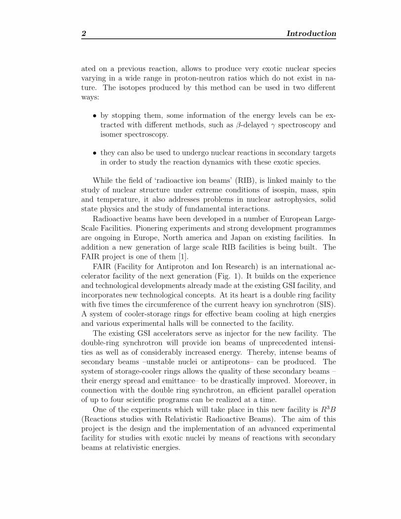
FAIR (Facility for Antiproton and Ion Research) is an international ac-celerator facility of the next generation (Fig. 1). It builds on the experienceand technological developments already made at the existing GSI facility, andincorporates new technological concepts. At its heart is a double ring facilitywith five times the circumference of the current heavy ion synchrotron (SIS).A system of cooler-storage rings for effective beam cooling at high energiesand various experimental halls will be connected to the facility.

The existing GSI accelerators serve as injector for the new facility. Thedouble-ring synchrotron will provide ion beams of unprecedented intensi-ties as well as of considerably increased energy. Thereby, intense beams ofsecondary beams –unstable nuclei or antiprotons– can be produced. Thesystem of storage-cooler rings allows the quality of these secondary beams –their energy spread and emittance– to be drastically improved. Moreover, inconnection with the double ring synchrotron, an efficient parallel operationof up to four scientific programs can be realized at a time.

One of the experiments which will take place in this new facility is R3B(Reactions studies with Relativistic Radioactive Beams). The aim of thisproject is the design and the implementation of an advanced experimentalfacility for studies with exotic nuclei by means of reactions with secondarybeams at relativistic energies.

Introduction 3

Figure 1: Schematic picture of the FAIR facility. In blue are shown theGSI existing facilities. In red are shown the new accelerator and the newexperimental areas. R3B will be placed dowstream the Super-FRS

The technical challenge of this project is to detect and fully identify inmass and charge and to determine the momenta of all the outcoming prod-ucts from the reactions induced by exotic nuclei. To achieve this aim, acomplex system of detection devices has been proposed. The measurementof the energy loss of the reaction products by ionization chambers allowsthe determination of the atomic number. This, combined with the use ofstrong magnetic fileds for determining the magnetic rigidity, together with adetermination of the velocity, will provide the mass number.

One of the possibilities considered for the velocity measurement is theuse of a Time-of-Flight (ToF) detector. Most of the detectors of this kindused until now for the identification of heavy ions were based on plasticscintillators coupled to photomultiplier tubes. However, the very sucessfuldevelopments in resistive plate chambers (RPCs), excellent time resolutionsand efficiencies close to 100 % have been achieved for MIPs. This fact, to-gether with the lower cost per electronics channel compared with scintillatortecnology, make this type of detectors a very encouraging alternative forvelocity determination with heavy ions.

The goal of this work is to define the performances of the ToF wall de-

4 Introduction

tector in order to satisfy the requirements (full acceptance and good timeresolution), investigate the possible present technologies to achieve this aimand propose a conceptual design based on the previous considerations. Thetwo possible technologies mentioned before have been considered: the useof fast scintillators coupled to ultra-fast phototubes and RPCs. In order toanalyze and discuss this two possibilities, we will divide the work in fourdifferent chapters.

• In the first chapter, an overview to the R3B project is presented, theexperimental setup and the detectors are described, as well as the ex-perimental method for the identification. We also discuss the detectorrequirements (time resolution, size and granularity).

• In the second chapter, the two most extended technologies for time-of-flight measurements, RPCs and plastic scintillators, are discussed.The performances of these two tecnologies in recent experiments arealso described.

• In the third chapter, a performance test of different readout methodsfor fast detectors is presented. These methods are the use of standardelectronics (TAC and ADC), complete digitation of the signal com-bined with later software analysis and the use of a complete new fastelectronics developed at GSI for the FOPI experiment [2].

• In the fourth chapter, a conceptual design for the construction of anRPC based Time-of-Flight wall which fulfills all the requirements isgiven.

Chapter 1

The R3B experiment

The goals of the R3B project are to design and implement an advancedexperimental setup for Reaction studies with Relativistic Radioactive ionBeams. The experiments will take place at the focal plane of the high energybranch of the Super FRS at the new FAIR facility in Darmstadt (Germany).The energies of the ion beams will be between 0.5 and 1 GeV per nucleon.

R3B will provide unique experimental conditions worldwide for experi-ments with relativistic secondary beams in order to benefit researchers inthe fields of nuclear structure physics, nuclear reaction physics and nuclearastrophysics.

1.1 Physics program at the R3B experiment

The different reaction types and associated physics goals that can beachieved at the R3B experimental setup are described in this section.

Total-absorption measurements. Nuclear matter radii may be inferredfrom total interaction cross sections derived from total-absortion mea-surements of radioactive ions in thick targets. These data together withisotope shift measurements, provide a first experimental manifestationof neutron skins [3].

Elastic-proton scattering. The radial distribution of nuclear density ofexotic nuclei may be extracted from high energy proton elastic scatter-ing. Previous experiments have demonstrated the power of the methodto investigate halos and skins in nuclei far off stability [4].

Knockout reactions. Break-up reactions induced by high-energy beams ofexotic nuclei allow the exploration of ground-state configurations and

6 The R3B experiment

of excited states. Knockout reactions have been used in particular tomap the halo nucleon wave function in momentum space, from whichtheir spatial distribution is derived via Fourier transformation [5].

Quasi-free scattering. R3B experiment intends to develop and apply thetechnique of quasi-free scattering using radioactive beams in inversekinematics. This type of reactions allows to extract information of thesingle-particle shell-structure, nucleon-nucleon correlations as well ascluster knockout reactions [6].

Electromagnetic excitation. Electromagnetic processes in heavy ion in-teractions at energies far above the Coulomb barrier give access to awealth of nuclear structure information on exotic nuclei. Surface vibra-tions and giant resonances can be studied [7].

Charge exchange reactions. The (p,n) charge exchange reaction can beused to excite Gamow Teller (GT) and spin dipole resonances. Studiesof the GT strength are beside their importance in nuclear structureof particular astrophysical interest. Electron-capture reactions lead-ing to stellar collapse and supernova formation are mediated by GTtransitions [8].

Fission. Since fission corresponds to a typical large-scale motion process,it has been recognised as one of the most promising tools for deduc-ing information on nuclear viscosity, and on shell effects and collectiveexcitations at extreme deformation [9].

Spallation reactions. Spallation reactions are important in various fieldsof research such as astrophysics, neutron sources and production ofradioactive beams [10].

Projectile fragmentation & multifragmentation. Heavy ions collisionsoffer the possibility to probe nuclear matter under extreme conditionsof densities and temperatures. Isotopic effects in multifragmentation,reflect the strength of the symmetry term in the equation of state.Projectile fragmentation of secondary beams in conjunction with γ-rayspectroscopy is a powerful method to explore excited states in exoticnuclei [11].

1.2 Layout of the experiment

For a complete kinematic measurement, all the particles coming out fromthe nuclear reaction have to be identified in mass and charge. Their momenta

1.2 Layout of the experiment 7

Figure 1.1: Schematic picture of the R3B experimental setup. From left toright, we can see the secondary target, the γ-detector, the large acceptancesuperconducting dipole magnet, three position detectors for tracking, the neu-tron detector (LAND), and a ToF wall for charged particles identification.At the bottom of the picture, the high resolution magnetic spectrometer forthe high resolution mode is shown.

have to be also measured very accurately. The proposed experimental setupis described in the following (Fig. 1.1).

Two modes of operation are foreseen depending on the demands of theexperiments:

Large acceptance mode: Heavy fragments and light charged particles aredeflected by a large acceptance dipole and detected with full solid-angleacceptance.

High resolution mode: Here, the dipole magnet is operated in reversedmode, deflecting the fragments into a high resolution magnetic spec-trometer.

The large gap of the dipole provides a free cone for the neutrons, whichare detected in forward direction by the Large Area Neutron Detector (newLAND).

The R3B proposal also includes the measurement of the emitted gammarays with a 4π γ-calorimeter around the target.

1.2.1 γ-ray detection

This detector should have high efficiency and good angular resolution. Itshould also have a high absortion probability for photons with energies up


to 10 MeV, due to the Lorentz boost of the γ-photons emitted. Besides theγ-sum, the calorimeter has to provide the γ-multiplicity and the individualγ-energies for spectroscopic purposes. Two design possibilities have beentaken into account. Either an array consisting on cooled scintillators (suchas CsI or NaI) or new inorganic scintillator materials, like LaBr3. The lightread-out will be performed by PIN diodes.

1.2.2 Neutron detection

The Large Area Neutron Detector has been designed for the detection ofhigh energy neutrons and determine their momenta via Time-of-Flight andposition measurement. An efficieny of more than 90% for 400 MeV neutronsand a time resolution in the order of 100 ps are required. Two possibletechnologies have been consireded in its design, either a sandwich of ironconverters and plastic scintillator or Resistive Plate Chambers (RPCs).

1.2.3 Light charged particles and ion detection

Atomic number determinaton

The measurement of the atomic number Z can be done with a MUlti Sam-pling Ionization Chamber (MUSIC), which consists on an ionization chamberwhose anode is segmented in several anode plates in order to achieve a betterresolution in charge determination [12].

Mass number determination

For the charged particles (e.g. protons and ions), the measurement of themagnetic rigidity, together with the velocity, makes possible their identifica-tion in mass-over-charge ratio (A/Q) according to the following equation:

Bρ =931.5

cγβ

A

Q(1.1)

where Bρ is the magnetic rigidity, γ is the Lorentz factor and β is the velocityof the ion. For measuring the Bρ, two different elements are needed: a largeacceptance dipole magnet, and a set of tracking detectors.

The characteristics of the different detectors are described in the thefollowing.

Dipole magnet. This superconducting dipole magnet has the followingparameters: a large vertical gap providing an angular acceptance of ±80

1.2 Layout of the experiment 9

mrad for neutrons, a maximum bending angle of 40, ensuring an acceptanceclose to 100% and a high field integral of about 5 Tm, which allows a bendingangle of 18 for a 15 Tm beam.

Tracking detectors. Three tracking detectors are needed in order to re-construct the trajectory of any particle through the dipole and determinetheir bending angle. One of these detectors will be placed in front of thedipole and the other two behind the magnet. This detectors should providea position resolution of 200 µm. Different types of detectors such as a TimeProjection Chamber (TPC), multiwire chambers or scintillating fibers arebeing considered as tracking detectors.

Velocity measurement

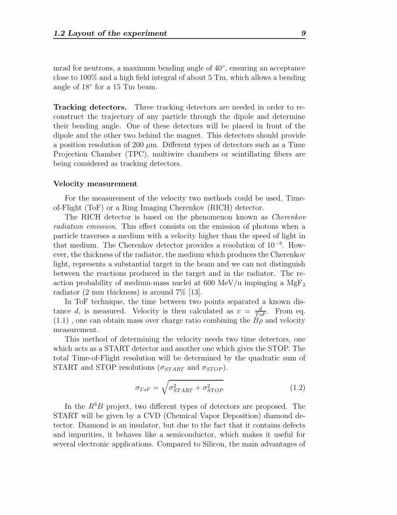
For the measurement of the velocity two methods could be used, Time-of-Flight (ToF) or a Ring Imaging Cherenkov (RICH) detector.

The RICH detector is based on the phenomenon known as Cherenkovradiation emission. This effect consists on the emission of photons when aparticle traverses a medium with a velocity higher than the speed of light inthat medium. The Cherenkov detector provides a resolution of 10−3. How-ever, the thickness of the radiator, the medium which produces the Cherenkovlight, represents a substantial target in the beam and we can not distinguishbetween the reactions produced in the target and in the radiator. The re-action probability of medium-mass nuclei at 600 MeV/u impinging a MgF2

radiator (2 mm thickness) is around 7% [13].In ToF technique, the time between two points separated a known dis-

tance d, is measured. Velocity is then calculated as v = dToF

. From eq.(1.1) , one can obtain mass over charge ratio combining the Bρ and velocitymeasurement.

This method of determining the velocity needs two time detectors, onewhich acts as a START detector and another one which gives the STOP. Thetotal Time-of-Flight resolution will be determined by the quadratic sum ofSTART and STOP resolutions (σSTART and σSTOP ).

σToF =√

σ2START + σ2

STOP (1.2)

In the R3B project, two different types of detectors are proposed. TheSTART will be given by a CVD (Chemical Vapor Deposition) diamond de-tector. Diamond is an insulator, but due to the fact that it contains defectsand impurities, it behaves like a semiconductor, which makes it useful forseveral electronic applications. Compared to Silicon, the main advantages of


diamond are a higher electron mobility and thus a fast signal, a high resistiv-ity which leads to a small leakage current (∼ few pA). But on the other hand,the number of electrons created by a charged particle is smaller in diamondthan in Silicon (36 against 89 per micron). The typical size of this type ofdetectors is of few cm2 and a thickness of hundreds of µm. The intrinsic timeresolution is 29 ps (σ) [14].

The STOP signal will be provided by a large area Time-of-Flight wall,based either on scintillators coupled to ultra fast photomultiplier tubes or onresistive plate chambers. The requirements of such a detector are describedin the next section.

1.3 Detector requirements for isotopic iden-

tification

As it was mentioned before, in order to perform a complete kinematicmeasurement of the reactions, all the particles created have to be completelyidentified (charge, mass, and momentum).

1.3.1 Charge and mass resolution

To identify the atomic number of the reaction products up to Z=92, oneneeds a relative resolution in charge of ∆Z/Z ∼ 0.5×10−2. This resolution iseasily reached with a MUSIC, which provides an accuracy of 0.3 charge unitsfor ions below Z = 80 [15]. In R3B experiment the MUSIC will be placedbetween the two last tracking detectors.

Once we have determined the atomic number, we need to separate thedifferent isotopes of a certain element. In order to be able to solve twoneighboring nuclei around the mass 200, a resolution in mass-to-charge ratio∆(A/Q)/(A/Q) ∼2.25×10−3 is required.

1.3.2 Magnetic rigidity and time-of-flight resolution

From eq. (1.1), one obtains:

(

∆(A/Q)

A/Q

)2

=1

(A/Q)2

[

(

∂(A/Q)

∂(Bρ)

)2

(∆(Bρ))2 +

(

∂(A/Q)

∂β

)2

(∆β)2

]

=

(

∆(Bρ)

Bρ

)2

+1

(1 − β2)2

(

∆β

β

)2

(1.3)

1.3 Detector requirements for isotopic identification 11

This expresion can be written in a different way by using the relationbetween β and ToF .

(

∆(A/Q)

A/Q

)2

=

(

∆(Bρ)

Bρ

)2

+ToF 4c4

((ToFc)2 − d2)2

(

∆(ToF )

ToF

)2

(1.4)

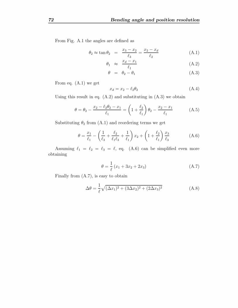
The accuracy in the determination of the magnetic rigidity, Bρ, is givenby the accuracy in the measurement of the bending angle,θ induced by thelarge dipole magnet.

∆θ

θ=

∆(Bρ)

Bρ(1.5)

This value is related to the resolution of the tracking detectors and themaximum magnetic field of the dipole.

∆θ =

√

(∆x1)2 + (3∆x2)2 + (2∆x3)2

`(1.6)

where ∆xi are the position resolution of the tracking detectors and ` is thedistance between them. ∆x2 has to take into account the angular stragglingin position detector 1. The straggling in the position detector 2 and theionization chamber has to be included in ∆x3. A detailed derivation of eq.(1.6) is shown in appendix A.

The resolution of the tracking detectors is assumed to be 200 µm. Thestraggling induced by the position detectors considering a distance around 1.2m between them is 0.19 mrad and 0.38 mrad for the MUSIC, this values havebeen calculated by using AMADEUS code [16], which allows to simulate theinteraction of relativistic heavy ions with matter. From eq. (1.6) we obtainthe value of the accuracy in the measurement of the bending angle θ for` = 1.2 m.

∆θ = 0.67 mrad

If we want to separate a fission fragment with atomic number Z = 64and mass around A = 160 at 600 MeV/u (Bρ = 10.137), the bending angle1

is θ = 226.24 mrad. This means that the resolution in magnetic rigidity,should be ∆Bρ

Bρ= 2.96 × 10−3. In order to achieve the required resolution

∆A/A ∼ 0.5/160 the time of flight should be determined with an accuracyaround 10−3. The time resolution required for mass A = 200 is slightly high(7×10−4) and depending on the distance between start and stop detectors(path-length, d), the absolute resolution needed will take diferent values, asshown in figure 1.2. As we can see the required resolution increases withthe mass of the nucleus we want to separate. For a 15 m pathlength, the

1The dipole magnet is designed to provide 18 for a 15 Tm beam


Mass Number100 120 140 160 180 200

To

F (

ps)

∆

20

40

60

80

100

1205 m

10 m

15 m

20 m

ToF resolution

Figure 1.2: Time of flight resolution needed to solve two neighbouring frag-ments at 700 MeV/u for different flight path-lengths and masses.

resolution needed to separate neighbouring isotopes, is ranging from 45.5 psof A = 200 to 95 ps of A = 100 (FWHM). This results allow us to considerthis distance as the most appropriate, due to the fact that the time resolutionneeded is achievable by using present technology. Time resolutions requiredfor shorter distances represents a challenge (σToF ≈ 10.9 ps for A = 200).For longer distances, the size of the detector makes too big, as shown in nextsubsection.

1.3.3 Size of the ToF detector

At first glance, the larger the path-length, the lower the time resolutionneeded, but we have to take into account other requirements. One of themis the size of the STOP detector. The main requirement is to cover the fullacceptance of the fragments produced in collisions induced by relativisticheavy ions. In order to estimate the size of the detector that fulfils thecondition, we are going to consider the reaction mechanism that covers thelarger angular range, fission.

Let us consider a 238U nucleus at 500 MeV/u which fissions in two frag-ments of charges Z1 = 20 and Z2 = 72 respectively. By using Wilkins model[17], we can obtain the value of the total kinetic energy avaliable in the center


of mass frame.

TKE =Z1Z2e

2

D(1.7)

D = r0A1/3

1

(

1 +2

3β1

)

+ r0A1/3

2

(

1 +2

3β2

)

+ d (1.8)

whereZ1, Z2, A1and A2 are the atomic numbers and the masses of the fissionfragments respectively. β1 = 0.6 and β2 = 0.6 are the deformation coeffi-cients. r0 = 1.16 fm, d = 2 fm.

By using momentum and energy conservation laws, the velocity of thefragments in center of mass frame can be obtained as.

vcm1

=

√

2A2TKE

A1(A1 + A2)vcm2

=A1

A2

vcm1

(1.9)

Once we have the modules of the velocities, the different space coordinatesare

v1

x = vcm1

sin θ cos φ v2

x = vcm2

sin θ sin φ (1.10)

v1

y = vcm1 cos θ v2

y = vcm2 sin(π − θ) cos φ (1.11)

v1

z = vcm1 sin(π − θ) sin φ v2

z = vcm2 cos(π − θ) (1.12)

where θ and φ are the polar and azimuthal angles in spherical coordinates.Due to the fact that the distribution is isotropic, in order to simplify thecalculations, we can take φ = 0. θ is also fixed to 90 because is the anglewhich will give the maximum angular aperture after a Lorentz tranformation.

A boost in the beam direction (z axis), will transform the velocities tothe laboratory frame.

vLABx =

vcmx

γ(

1 + ~v·~βc

) vLABz =

βc(

1 + ~v·~βc

) (1.13)

The angle between the velocity vector and the beam line can be calculatedas

θLAB = arctan

(

vLABx

vLABz

)

(1.14)

With this simple calculation, one can estimate the size of the detector.The fragments produced by fissioning 238U nuclei at 500 MeV/u, will beemitted with a maximum angle in the laboratory frame of θLAB ≈ 53.4


d (m) size(m)

5 0.54

10 1.07

15 1.60

20 2.13

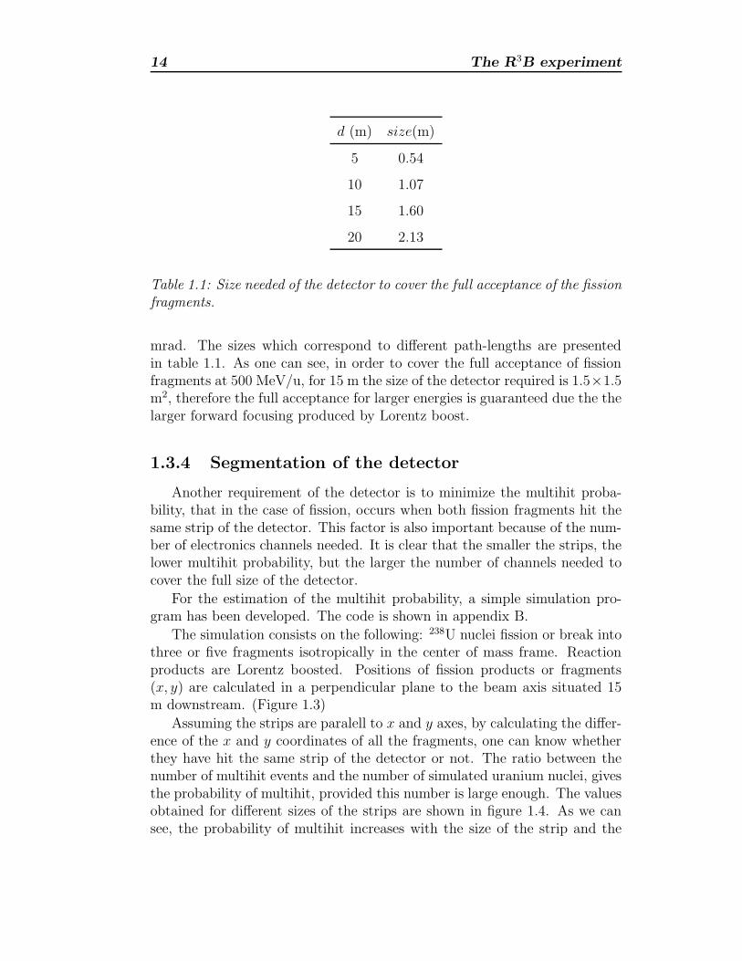
Table 1.1: Size needed of the detector to cover the full acceptance of the fissionfragments.

mrad. The sizes which correspond to different path-lengths are presentedin table 1.1. As one can see, in order to cover the full acceptance of fissionfragments at 500 MeV/u, for 15 m the size of the detector required is 1.5×1.5m2, therefore the full acceptance for larger energies is guaranteed due the thelarger forward focusing produced by Lorentz boost.

1.3.4 Segmentation of the detector

Another requirement of the detector is to minimize the multihit proba-bility, that in the case of fission, occurs when both fission fragments hit thesame strip of the detector. This factor is also important because of the num-ber of electronics channels needed. It is clear that the smaller the strips, thelower multihit probability, but the larger the number of channels needed tocover the full size of the detector.

For the estimation of the multihit probability, a simple simulation pro-gram has been developed. The code is shown in appendix B.

The simulation consists on the following: 238U nuclei fission or break intothree or five fragments isotropically in the center of mass frame. Reactionproducts are Lorentz boosted. Positions of fission products or fragments(x, y) are calculated in a perpendicular plane to the beam axis situated 15m downstream. (Figure 1.3)

Assuming the strips are paralell to x and y axes, by calculating the differ-ence of the x and y coordinates of all the fragments, one can know whetherthey have hit the same strip of the detector or not. The ratio between thenumber of multihit events and the number of simulated uranium nuclei, givesthe probability of multihit, provided this number is large enough. The valuesobtained for different sizes of the strips are shown in figure 1.4. As we cansee, the probability of multihit increases with the size of the strip and the


x position (cm)-60 -40 -20 0 20 40 60

y p

osi

tio

n (

cm)

-60

-40

-20

0

20

40

60

0

2

4

6

8

10

12

position distribution of the frangments xVSy

Figure 1.3: Distribution of position of the fission fragments in the STOPdetector at 15 m downstream.

Strip size (cm)0 2 4 6 8 10 12 14

Pro

bab

ility

(%

)

0

10

20

30

40

50

60

70

80

Fission3 fragments5 fragments

Multihit Probability

Figure 1.4: Probability of Double hit for different sizes of the strips of thedetector for 15 m pathlength. As we can see, a stripsize of 5 cm, givesprobabilities lower than 10% for fission and multifragmentation reactions.

multiplicity of the events. For 5 cm strips, the probability of double hit islower than 10 % in all cases, reaching less than 1% for the fission. Therefore,


this stripsize seems the most appropriate. Smaller strips would require toomuch electronic channels.

1.4 Physical limitations to the velocity reso-

lution

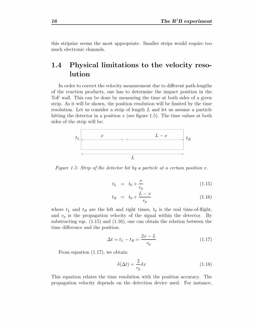
In order to correct the velocity measurement due to different path-lengthsof the reaction products, one has to determine the impact position in theToF wall. This can be done by measuring the time at both sides of a givenstrip. As it will be shown, the position resolution will be limited by the timeresolution. Let us consider a strip of length L and let us assume a particlehitting the detector in a position x (see figure 1.5). The time values at bothsides of the strip will be:

PSfrag replacements

tL tR

L

x L − x

Figure 1.5: Strip of the detector hit by a particle at a certain position x.

tL = t0 +x

vp(1.15)

tR = t0 +L − x

vp(1.16)

where tL and tR are the left and right times, t0 is the real time-of-flight,and vp is the propagation velocity of the signal within the detector. Bysubstracting eqs. (1.15) and (1.16), one can obtain the relation between thetime difference and the position.

∆t = tL − tR =2x − L

vp(1.17)

From equation (1.17), we obtain:

δ(∆t) =2

vp

δx (1.18)

This equation relates the time resolution with the position accuracy. Thepropagation velocity depends on the detection device used. For instance,

1.5 Proposed requirements for the ToF wall detector 17

Atomic Number20 30 40 50 60 70 80 90

(x)

(mm

)∆

0

2

4

6

8

10

12

14

16 3 m

8 m

13 m

Position resolution due to angular straggling in air

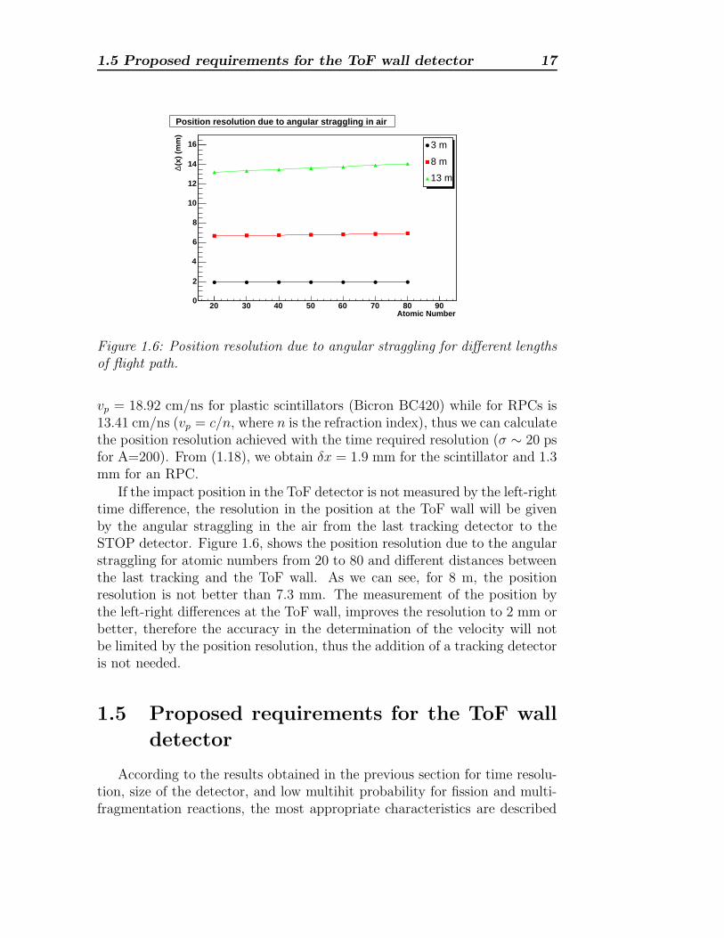
Figure 1.6: Position resolution due to angular straggling for different lengthsof flight path.

vp = 18.92 cm/ns for plastic scintillators (Bicron BC420) while for RPCs is13.41 cm/ns (vp = c/n, where n is the refraction index), thus we can calculatethe position resolution achieved with the time required resolution (σ ∼ 20 psfor A=200). From (1.18), we obtain δx = 1.9 mm for the scintillator and 1.3mm for an RPC.

If the impact position in the ToF detector is not measured by the left-righttime difference, the resolution in the position at the ToF wall will be givenby the angular straggling in the air from the last tracking detector to theSTOP detector. Figure 1.6, shows the position resolution due to the angularstraggling for atomic numbers from 20 to 80 and different distances betweenthe last tracking and the ToF wall. As we can see, for 8 m, the positionresolution is not better than 7.3 mm. The measurement of the position bythe left-right differences at the ToF wall, improves the resolution to 2 mm orbetter, therefore the accuracy in the determination of the velocity will notbe limited by the position resolution, thus the addition of a tracking detectoris not needed.

1.5 Proposed requirements for the ToF wall

detector

According to the results obtained in the previous section for time resolu-tion, size of the detector, and low multihit probability for fission and multi-fragmentation reactions, the most appropriate characteristics are described


in the following.The ToF wall should be placed around 15 m downstream from the target.

The angular straggling produced by 8 m of air from the last tracking detectorto the ToF wall will not limit the velocity resolution required. The resolutionachieved in the position from left-right time differences is lower than 2 mm.The time accuracy needed to separate masses around A ∼ 200 at 700 MeV/ufor 15 m pathlength is σToF ≈ 20 ps. Due to the fact that diamond detectors’intrinsic time resolution is σ = 29 ps, the resolution will be limited by thisvalue. Other possible detectors should be considered as START in order toavoid this limitation. As far as size is concerned, the one required to coverthe full acceptance for fission fragments is 1.5× 1.5 m2. The detector will bedivided in strips of 5 cm, providing a multihit probability lower than 10%for multifragmentation reactions (5 fragments).

Two different technologies can be used to implement such a detector:Resistive Plate Chambers (RPC), or fast plastic scintillators attached to fastphotomultiplier tubes. Both methods will be explained in detail in the nextchapter.

Chapter 2

Time-of-Flight detectors.

In this chapter, two different kinds of detectors for the R3B large areaToF wall are presented, organic scintillators coupled to fast photomultipliertubes (PMTs), and resistive plate chambers (RPCs). Both technologies arethe most extendend nowadays for time-of-flight measurements. Here we willpresent both types of detectors and we will discuss their performances forToF measurements.

2.1 Resistive plate chambers (RPCs)

These detectors were introduced in 1981 [18] as a practical alternativeto the remarkable ‘localized discharge spark counters’ developed by Pestov[19], which provides a very good time resolution (σ ∼ 25 ps). Their maindifference is that RPCs work at atmosferic pressure, while the Pestov counterrequires higher pressures. Another drawback of the Pestov detectors is thefact that the gas mixture used is flammable.

2.1.1 Fundamentals of resistive plate chambers

RPCs are gaseous detectors with a uniform electric field produced by twoparalell electrode plates, one of which —at least— is made of a materialwith high bulk resistivity. The gap between the two electrodes, rangingfrom a few hundred micron to millimeters, depending on the application,is filled with a gas mixture with a high absortion coefficient for ultravioletphotons and very good electron affinity. The electrons and the ions createdby the incoming particle are accelerated towards the anode and the cathode,respectively. When the primary ionization gains enough energy to ionizeother gas molecules, secondary electrons are created. This new electrons can

20 Time-of-Flight detectors.

produce new ionizations, leading to the formation of an avalanche. The totalnumber of electrons created in a path x, is [20]:

n = n0 exp (αx) (2.1)

where n0 is the initial number of electrons and α is the first Townsed coeffi-cient. The factor eαx, known as multiplication factor, is limited to about 108

or αx = 20 (Raether’s limit) [21]. Above this value, a continuous dischargeregime can be generated with spark production.

Pulse formation

As the electrons and ions drift towards the anode and cathode respec-tively, a pulse signal is induced in the electrodes. These signals are pickedup by a readout system.

Discharge quenching

In RPCs, the discharge is quenched by the following mechanisms:

1. prompt switching off of the field around the discharge point, due to thelarge resistivity of the electrodes: the duration of the discharge is muchshorter than the relaxation time of the electrode plates [22], which isof the order of ρε = τ ≈ 2 s for glass (ρ and ε are the resistivity andelectrical permitivity). Therefore, the charge needed for furnishing aspark cannot flow fast enough.

2. UV photon absortion by the gas, preventing secondary discharges fromgas photoionization.

3. Capture of the outer electrons of the discharge due to the electronaffinity of the gas mixture, which reduces the size of the discharge andpossibly its transversal dimensions.

Rate capability

The high resistance of the electrodes, which avoids sparks and other dan-gerous processses (like permanent discharges) represents on the other handone of the main limitations of this detectors. After the signal is produced, thecharge of the avalanche stays on top of the electrode and during this time theeffective field in the region where the avalanche develope will be lower. Asa consequence, if the counting rate is very high, one can expect fluctuationsin the local field caused by earlier avalanches. The main consequence is areduction of the efficiency and the time resolution.

2.1 Resistive plate chambers (RPCs) 21

Modes of operation

RPCs may be operated either in avalanche mode or in streamer mode:

- The avalanche mode corresponds to the generation of a Townsed avalanchein the gas gap, following the release of primary charges by the incomingradiation. Because of the low amplification of the gas mixtures usedin this mode, the gain has to be compensated by using high-gain fastamplifiers integrated in the front-end-electronics (FEE)[23].

- The streamer mode requires higher operation voltages than the avalanchemode. In this case, the secondary ionizations, caused by photons emit-ted by excited gas molecules, are so large that the space charge createddistorts the electric field, causing eventually a discharge in the detectorgas. Quenching gases are added to control and localize this discharge.On the one hand, this approach has the advantage of providing largersignals that can be discriminated without amplification. However, dueto high resistivity of the electrodes, the area were the streamer devel-opes is blind during a given transit time [24].

Originally, RPCs have been operated in the streamer mode. Later on, re-markable progress was achieved in the avalanche mode operation, providingbetter rate capability of the RPCs. At present, most of the RPCs used fortiming operate in avalanche mode.

RPC designs

Single gap RPC. The original RPC [18], had a single gas gap delimitedby bakelite resistive electrodes. These counters has evolved since then.Glass electrodes, having a mechanical rigidity and surface quality muchsuperior to bakelite, are being used in recent designs.

Multigap RPC. This construction method has been proposed in 1996 [25].It consists on a stack of equally-spaced resistive plates that divide thegas volume into a number of individual gaps. High voltage is appliedto external surfaces. Initially, internal plates take correct voltage, fromelectrostatics, then they are kept at correct voltage by flow of electronsand positive ions created by the avalanches in the gaps. This feedbackprinciple produces a similar gain in all gas gaps. Due to the fact thatresistive plates are transparent to fast signals, the readout is done atthe most external plates [24]. This design presents an improvement inthe efficiency and time resolution. A possible drawback of this designare the high voltages required.


Multigap RPCs have been used to construct large area time-of-flight detec-tors [26] delivering a time resolution of the order of σ(ToF ) < 60 ps forminimum ionizing particles (MIPS). Some examples are the ToF detectorsfor the ALICE [27], STAR [28], HADES [29] or FOPI [2] experiments.

ALICE and STAR use a very similar approach for their timing RPCs.Both designs consist on multigap glass RPCs, where the pickup pads aredeposited in a Printed Circuit Board (PCB).

In the ALICE detector, an element consists on a long RPC strip (120×7.4cm2) with 96 readout pads arranged in two rows. The strip is made of 2 stacksof 5 gaps of 250 µm each. The resistive plates are commercial glass 400 µmthick for the internal and 550 µm for the external plates; the distance betweenthem is kept fixed with spacers made of nylon fishing line. The anode is in themiddle and the two cathodes are on the external surfaces. For the readout,a differential signal is obtained from the cathode and anode pads.

In the STAR experiment, an RPC element is made of six pads. The sizeof each pad is 3.1×6.0 cm2. The glass plates are 520 µm thick. There are sixgaps of about 220 µm . The electrodes are made of graphite and the readoutis done in the pads.

In the FOPI experiment, an RPC module consists on a 16 strip anodewith an active width of 4.6 cm and a length of 90 cm. The gap size is 300µm with glass plates of 1.1 mm thickness. The shape of the strips has beenadapted to the readout cables in order to match the impedance to 50 Ω.

HADES design is slightly different. It consists on glass and aluminiumRPC cells of 4 gaps of 300 µm width. This hybrid design is more appropriatefor this experiment, due to the higher rates which can be tolerated by thesetype of detectors. The cells are electrically isolated in order to prevent thecrosstalk.

2.1.2 Performances of RPCs

Performances of resistive plate chambers, namely time resolution andefficiency, are determined by different factors such as the gas mixture, thenumber of gaps, the gap width and the operation voltage. The readoutelectronics plays also an important role in the time resolution.

Gas mixture

Modern standard RPCs working in avalanche mode use mostly mixturesof tetrafluoroethane (C2H2F4) with 2% to 5% of isobutane (iso-C4H10) and0.4% to 10% of sulphur hexafluoride (SF6). The addition of SF6 has beenshown to extend the streamer free operation region [30]. By increasing the


fraction of SF6, the efficiency plateau shifts to higher voltages. The timeresolution is defined by to competing processes with increasing SF6 con-centration. Large fractions of this gas require higher electric fields. As aconsequence, a higher drift velocity if expected, which results in an improvedtime resolution. On the other hand, SF6,can capture all electrons in a clusterof ionization due to the large capture cross-section for low energy electrons,. Thus, by increasing the concentration of SF6, the number of ionizationclusters that generate an avalanche is reduced, leading to a degradation ofthe time resolution and efficiency (Fig. 2.1).

Figure 2.1: Efficiency (top) and time resolution (bottom) for different SF6

fractions used in the gas mixture [30].

Size and number of gaps

The size of the gap is a factor that determines, in a significative way,the efficiency and the time resolution that can be achieved with an RPCdetector. The larger the gap, the higher the efficiency. Gaps of around 2


mm were used in the first designs [18] and are used nowadays in the so-calledtrigger RPCs, operated either in avalanche or streamer mode. This type ofdetectors have reached efficiencies above 98% per gap, independently of theoperation mode. The time resolution achieved is between 1 and 1.5 ns (σ).

Thinner gaps show a reduced efficiency (ε = 75%), but the time resolu-tion increases in a significative way. Resolutions better than 90 ps (σ) havebeen obtained using gaps ranging from 200 to 300 µm. On the other hand, itwas observed that for gaps smaller than 200 µm, apart from the mechanicaldificulties, such as the uniformity of the gap, the time resolution deterio-rates. By using multigap RPCs one can improve the efficiency in small gapchambers. In fact, the efficiency increases with the number of gaps as [24]:

ε = 1 − (1 − εg)n (2.2)

where ε is the total efficiency, εg is the efficiency of one gap, and n is thenumber of gaps. The time resolution also improves but with

√n.

Operation voltage

Another important factor which determines the performances of an RPCis the electric field. Timing RPCs work at fields of 100 kV/cm. The higherthis value, the larger the drift velocity and therefore the better the timeresolution achieved. The efficiency is also higher with high voltages. It hasalso to be taken into account that the probability for streamers increases withthe voltage. The working point will be a compromise between these factors:high efficiency, good time resolution and low probability of streamers.

Time-charge correlations

In order to achieve the best possible time resolution avaliable with anRPC, a measurement of the charge induced by the electrons is needed. Thischarge value is correlated with the time, due to the physics of the RPC[28]. The procedure for substracting this dependence is often called ’slewingcorrection’. See figure 2.2 for a sample of this correlation.

Figure 2.3, shows the efficiency, time resolution and streamer probabilityas a function of the high voltage applied to electrodes for five gaps RPC [27].As we can see the efficiency reaches 99.9%, and the time resolution is in the40 ps (σ) range. Streamers appear for voltages higher than 13 kV in thisdesign.

In table 2.1 a survey of the published results concerning the performancesof RPC detectors is shown. All these results concern multigap RPCs witha gas gap ranging from 220 to 300 µm. All the efficiencies reached are


Figure 2.2: The time amplitude correlation for cosmic rays with a multigapRPC (300 µm, gap width) at 14 kV voltage operation. Standard mixture hasbeen used [28].

Figure 2.3: Efficiency, time resolution (σ) and streamer probability for aMultigap RPC [27].

higher than 90%. Results concerning time resolution vary from the 48 ps (σ)obtained for the ALICE RPCs [27] to the 90 ps obtained by STAR experiment[28]. It should be noted that all these results have been measured using MIPS,


Voltage (kV) Gap width (µm) Number ε (%) Time Resolution Ref.

of gaps σ (ps)

14 220 6 90 90 [28]

9.5 300 6 97 <73 [2]

12 250 10 99.9 48 [27]

6.2 300 4 97 67 [29]

Table 2.1: Reported performances of recent RPC counters. The gas mixtureused in all cases is the standard one.

except for [29], where the fragmentation products of 12C at 1 GeV/u whereused.

Read-out electronics

Read-out electronics is also an important element in the time resolutionwhich can be achieved with RPC detectors. This is due to the fact that theintrinsic time resolution of RPCs is very good (σi ≈ 25 ps)[31], thereforethe total time resolution will be a quadratic sum of the intrinsic and theelectronics resolution. Different electronics have been developed in order tominimize this contribution to the total time resolution.

STAR and ALICE experiments used a front-end-electronics (FEE) basedin the MAXIM3760 amplifier [32, 28]. Due to the power used by this device(300 mW), people working at ALICE designed a new ultra fast and low power(40 mW/channel) FEE, rejecting MAXIM design. Readout is performedwith a high performace TDC developed at CERN [31] whose time resolutionis about 20 ps.

For the FOPI experiment, a complete FEE and digitazion card has beendeveloped (TAQUILA)[2]. The time resolution of this new electronics isbetter than 30 ps.

RPCs and heavy ions

Very little is known about the performance of RPCs for highly ionizingparticles such as heavy ions. It has been reported that in fragmentationexperiments of 12C [29] the capabilities of such detectors is not significativelydegraded. A resolution of 67 ps (σ) and efficiency of 97% have been reachedfor a 4-gap glass aluminium RPC.

2.2 Scintillation detectors 27

For heavier ions, ionization is expected to increase as Z2, Z is the atomicnumber of the ion, two effects have to be studied:

• energy losses in the electrodes should not be enough to stop the ion.

• the highly primary ionization would imply necessary a lower field, andsubsequently in a reduced value of Townsed first coefficient and driftvelocity, so the final resolution achievable will be a competition betweenthese two effects. Efficiency can always be improved just by usingadditional gaps.

2.2 Scintillation detectors

Scintillation detectors are one of the most widely used particle detectiondevices in nuclear and particle physics. They are based on the fact thatcertain materials when struck by an ionizing radiation, emit a small flash oflight, i.e. a scintillation.

2.2.1 General features

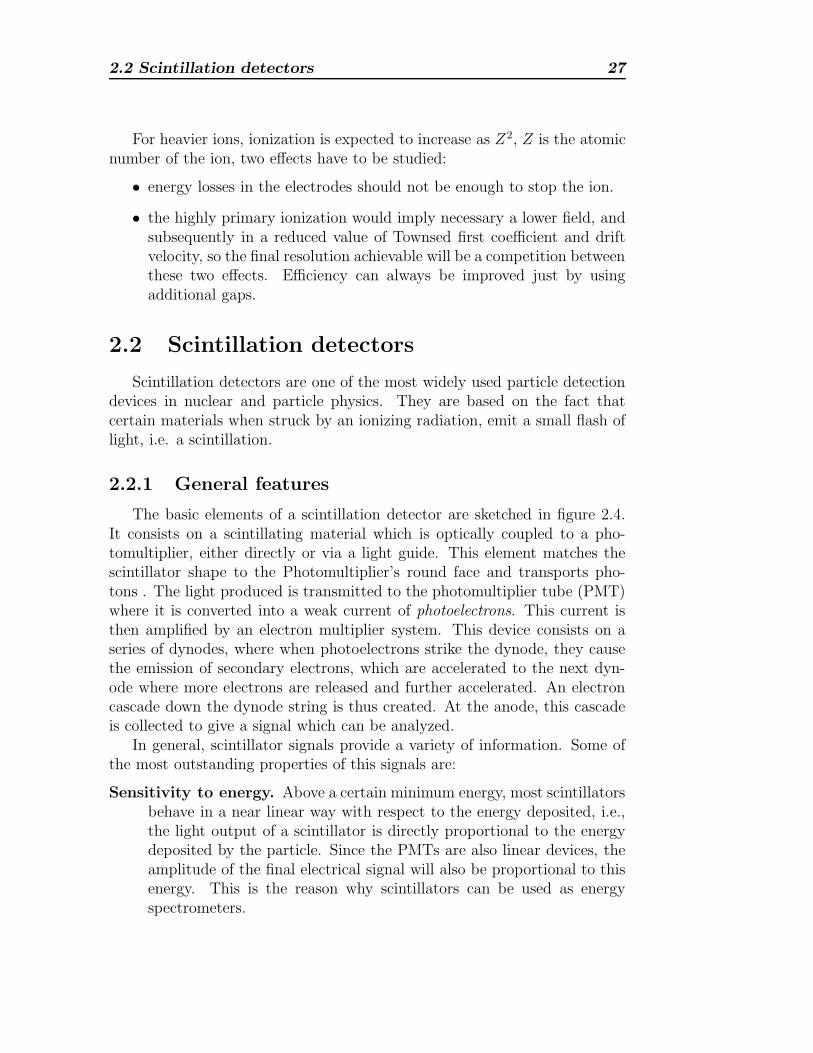
The basic elements of a scintillation detector are sketched in figure 2.4.It consists on a scintillating material which is optically coupled to a pho-tomultiplier, either directly or via a light guide. This element matches thescintillator shape to the Photomultiplier’s round face and transports pho-tons . The light produced is transmitted to the photomultiplier tube (PMT)where it is converted into a weak current of photoelectrons. This current isthen amplified by an electron multiplier system. This device consists on aseries of dynodes, where when photoelectrons strike the dynode, they causethe emission of secondary electrons, which are accelerated to the next dyn-ode where more electrons are released and further accelerated. An electroncascade down the dynode string is thus created. At the anode, this cascadeis collected to give a signal which can be analyzed.

In general, scintillator signals provide a variety of information. Some ofthe most outstanding properties of this signals are:

Sensitivity to energy. Above a certain minimum energy, most scintillatorsbehave in a near linear way with respect to the energy deposited, i.e.,the light output of a scintillator is directly proportional to the energydeposited by the particle. Since the PMTs are also linear devices, theamplitude of the final electrical signal will also be proportional to thisenergy. This is the reason why scintillators can be used as energyspectrometers.


Figure 2.4: Schematic view of a typical scintillation detector.

Fast time response Scintillation detectors are fast instruments in the sensethat their response and recovery times are short relative to other typesof detectors. This fast response makes their use suitable for timingmeasurements. This feature, together with their fast recovery timealso make this detector suitable to accept high counting rates (thedecay time of plastic scintillators is τ ∼ 1 ns).

While many scintillating materials exist, not all are suitable as detectors.In general, a good detector scintillator should satisfy the following require-ments:

1. high efficiency for conversion of exciting energy to fluorescent radiation

2. transparency to its fluorescent radiation and consequently good trans-mission of the light

3. emission in a spectral range consistent with the spectral response ofexisting PMTs.

Nowadays two kinds of scintillator materials are in use: inorganic crystalsand organic scintillators. The first ones are slower, but they have excellentproperties for γ-detection. Organic scintillators are discussed in the nextsubsection.

2.2.2 Organic scintillator materials

Organic scintillators are aromatic hydrocarbon compounds containinglinked or condensed benzene-ring structures. Their most interesting featureis a very rapid decay time, on the order of few nanosecons or less [21, 20].This is the reason why these materials are suitable for time measurements.

Scintillation light in these compounds arises from the transitions made byfree valence electrons of the molecules. Ionization energy from penetrating

2.2 Scintillation detectors 29

Scintillator(BICRON)

PMT(HAMAMATSU)

σ (ps) Ref

BC422Q(0.5%) R4998 8.9 [33]

” R2083 11.2 [33]

” R3809U 24.8 [33]

” R5900-L16 19.8 [33]

BC404 R6504S 49 [35]

BC408 R2490-05 50 [34]

BC420 R2431 75 [9]

Table 2.2: Time resolution achieved with scintillators in different experi-ments

radiation excites both the electron and vibrational levels. Because of theenergy lost by vibrational quanta, emission and absorption spectra are shiftedin wavelength, thus scintillator is transparent to the light it produces.

Due to the molecular nature of luminescence in these materials, organicscintillatros can be used in many physical forms without the loss of theirscintillating properties. As detectors, they have been used in the form ofpure crystals and as mixtures of one or more compounds in liquid and solidsolutions.

2.2.3 Performances of scintillation detectors

Organic scintillators have been the most used detectors in ToF masure-ments. Recently the development of new fast plastic scintillators and ultra-fast photomultiplier tubes, has allowed reaching very good time resolutions[33, 34, 35].

A survey of the latest results obtained for the time resolution with scin-tillation detectors is presented in table 2.2.

As we can see, the best results correspond to reference [33], where thetime resolution achieved for 40Ar at 95 MeV/u is betterlower than 20 ps (σ),reaching 9 ps for a specific scintillator (BC422Q) and PMT HAMAMATSUR4998. It should be taken into account that these measurements have beenperformed using small detectors (about 50 mm long). In a realistic envi-ronment, the size of the scintillator should be large enough to cover a largeacceptance. Also, it would be important to keep the distance between the


beam line and the PMTs to avoid extra radiation damage of the tubes. Notso good time resolution is expected for a larger scintillators due to the re-suction of the number of photons transmited to the PMT. The thickness ofthe scintillators was 0.5 mm. In principle, the use of thinner material inthe beam line is required in order to avoid extra interactions and energystraggling of the incident beam. In contrast, with this requirement, timeresolution decreases due to the reduction of the photon emission. In fact,the time resolution is related to the number of photoelectrons (Np.e.) by thefollowing empirical relation [33]:

σT ∝ (Np.e.)α (α = −0.5) (2.3)

The type of the PMT plays an important role in the time resolutionobtained with scintillation detectors (see table 2.2). Comparing the excellenttime resolution obtained with the R4998 and the R2083 PMTs, a resolutionmuch worse is obtained with the R3809U and R5900-L16 despite of the fastertiming response (0.15 and 0.6 ns risetime versus 0.7 ns). This might be dueto the very fast time response of the R3809U photomultiplier relative to thetime duration of the scintillating light. This fact suggests the importance ofselecting the scintillation materials and the PMTs considereing the matchingof their properties.

The time resolution due to electronics (discriminator and TDC) con-tributes to the total time resolution. In Ref. [33], this contribution hasalso been estimated and its value is better than 8 ps (σ), very close to theTDC precision (7.2 ps σ). Therefore the precision of the electronics becomesnot negligible for a high resolution ToF scintillation detector below 10 ps.

The result of reference [34] correspond to a more realistic setup. Thebeam used was 2 GeV π−. The scintillators were 165 and 130 cm long with adouble layer configuration. The thickness of each plastic was 5 cm allowinga better statistics of photoelectrons. The use of a double layer system allowsa better time resolution than a single one (65 and 50 ps σ respectively).

In [35], the resolution achieved with a 95×10×2 cm2 if 49 ps for negativepions. The readout electronics consisted on an ADC (LeCroy 2249 W, 0.25pC/count) a TDC (Phillips 7186, 25 ps/count) and a discriminator (Phillips708).

It should be taken into account that these resolutions have been obtainedby using the time-walk correction of signals. This correction is due to thepulse height variations. The times measured are corrected by the integratedcharge of the PMT by:

T = T raw − Cwalk

√q

(2.4)

2.3 Summary and conclusions 31

where T is the corrected time, T raw the uncorrected time, Cwalk the correctionfactor and q the integrated charge of pulse. Results of [9], correspond to theresolution achieved for fission fragments. The size of the scintillator used was1m long.

2.3 Summary and conclusions

Resistive Plate Chambers and scintillator detectors are very suitable de-vices for the measurent of the time-of-flight of residues produced in nuclearreactions induced by relativistic heavy ions. The efficiency and time resolu-tion achieved with the ‘state of the art’ timing RPCs, multigap glass RPCs ina range of 0.2-0.3 mm gap width, is about 99% and 50 ps (σ) respectively forMIPS. These results are very encouraging for the use of these type of detec-tors in the identification of heavy ions by time-of-flight measurements, as analternative to the standard scintillation detectors. Scintillators have shownexcellent performances for new scintillation materials and photomultipliertecnologies.

Recent experiments [2, 27, 28, 29] have implemented large area ToF wallsbased on RPC technology due to very good performances and the lower costper channel compared with the scintillator option.

However, further studies should be performed in order to investigate theperformances of RPCs with heavy ions.

Chapter 3

Performance tests of differentread-out electronics

In this chapter are presented the results obtained in the evaluation ofdifferent solutions proposed for the readout of the signals induced by heavyions in plastic scintillators and RPC detectors, in order to achieve the timeresolution required for the ToF wall (Sect. 1.3).

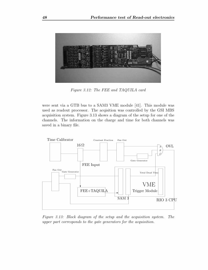
The first option is the use of standard modular electronics (Discrimina-tors, TAC and ADC). Another possibility is a complete digitation of thesignals produced by fast scintillators and PMTs and an offline analysis ofthem with software tools. The last possible solution is the use of integratedelectronics, in particular the TAQUILA card developed by the Electronicsdepartment at GSI [2].

3.1 Standard modular electronics

The first option we have evaluated is the use of standard modular elec-tronics (NIM and VME) for the readout of the signals.

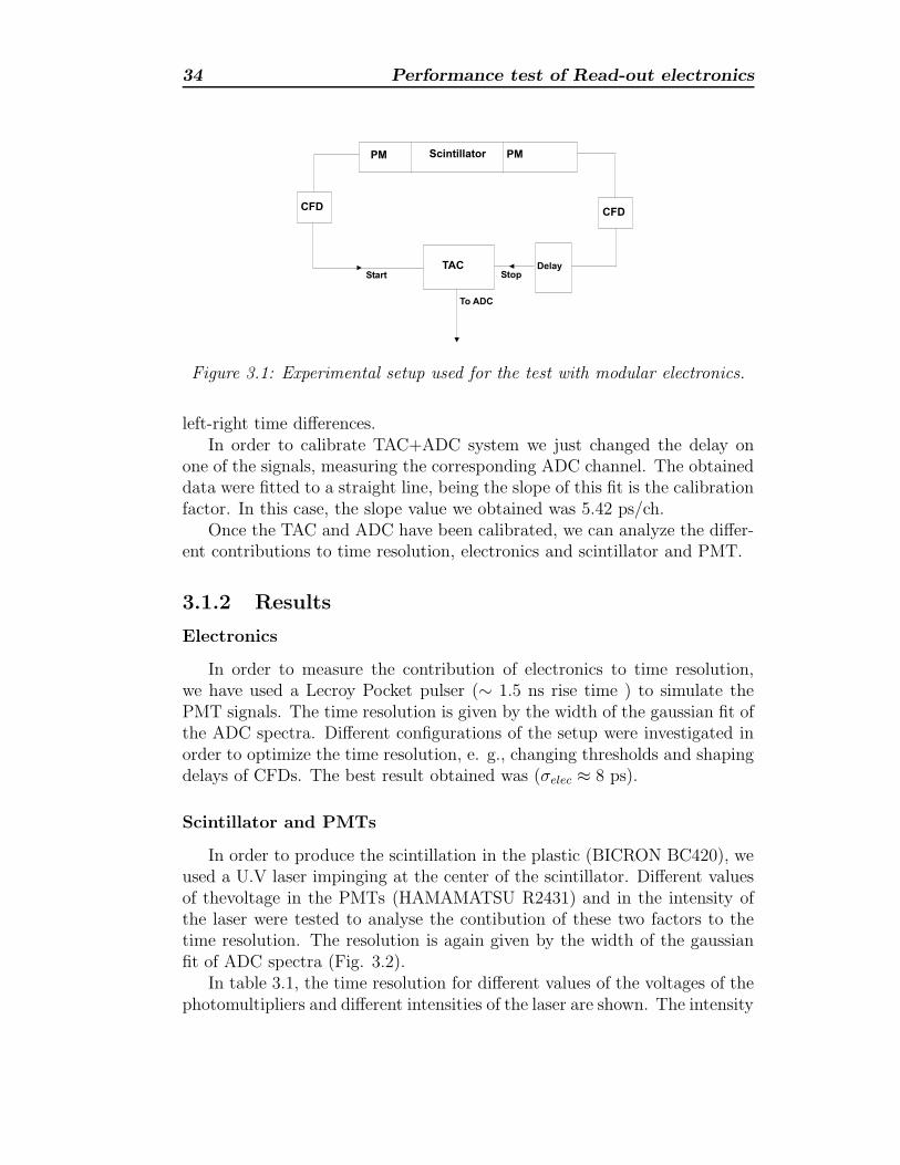
3.1.1 Experimental Setup

In order to measure the time resolution that can be achieved with thismethod, we used the setup shown in figure 3.1 The signals produced in bothPMTs were sent to ORTEC constant fraction dicriminators (CFD) [36]. Oneof the signals was delayed before being sent to the Time to Amplitude Con-verter (TAC) as STOP signal. The other pulse was used as START. TheTAC output is sent to an Analog to Digital Converter (CAEN V785 ADC)for on-line analisys of the distributions of TAC amplitudes, given by the

34 Performance test of Read-out electronics

ScintillatorPM PM

TAC

CFD

Start Stop

To ADC

Delay

CFD

Figure 3.1: Experimental setup used for the test with modular electronics.

left-right time differences.In order to calibrate TAC+ADC system we just changed the delay on

one of the signals, measuring the corresponding ADC channel. The obtaineddata were fitted to a straight line, being the slope of this fit is the calibrationfactor. In this case, the slope value we obtained was 5.42 ps/ch.

Once the TAC and ADC have been calibrated, we can analyze the differ-ent contributions to time resolution, electronics and scintillator and PMT.

3.1.2 Results

Electronics

In order to measure the contribution of electronics to time resolution,we have used a Lecroy Pocket pulser (∼ 1.5 ns rise time ) to simulate thePMT signals. The time resolution is given by the width of the gaussian fit ofthe ADC spectra. Different configurations of the setup were investigated inorder to optimize the time resolution, e. g., changing thresholds and shapingdelays of CFDs. The best result obtained was (σelec ≈ 8 ps).

Scintillator and PMTs

In order to produce the scintillation in the plastic (BICRON BC420), weused a U.V laser impinging at the center of the scintillator. Different valuesof thevoltage in the PMTs (HAMAMATSU R2431) and in the intensity ofthe laser were tested to analyse the contibution of these two factors to thetime resolution. The resolution is again given by the width of the gaussianfit of ADC spectra (Fig. 3.2).

In table 3.1, the time resolution for different values of the voltages of thephotomultipliers and different intensities of the laser are shown. The intensity

3.2 Signal digitation and pulse shape analysis 35

0

20

40

60

80

100

120

140

160

2100 2105 2110 2115 2120 2125 2130 2135 2140Ch. No.

No.

of

even

ts

0

50

100

150

200

250

2100 2110 2120 2130 2140 2150Ch. No.

No.

of

even

tsFigure 3.2: ADC spectra for the scintillator and PMTs. Sigma is the widthof the distribution times the calibration factor.

of the laser is determined by the amplitude of the output signal. As we cansee, the higher the light intensity, the better the time resolution achieved.This observation is in agreement with eq.(2.3), since a higher light intensityproduces a larger number of photoelectrons. One can also see that the timeresolution does not improve by increasing the voltage. This fact might be dueto the appearance of noise in the phototube. Therefore the time resolutionestimated for the scintillator and PMT system is around σ ≈ 8 ps.

3.2 Signal digitation and pulse shape analysis

As mentioned before, this method is based on the complete digitation ofthe pulses produced by the detector and the analysis of these pulses by meansof software applications. This procedure has been used in recent experiments[37] and represents the state-of-the-art in data analysis and discriminationtechniques.

In this section we present the results obtained in the analysis of the pulsesproduced by plastic scintillators coupled to fast photomultiplier tubes. Wealso analyzed the signals produced by a Lecroy pocket pulser in order todistinguish between the two different contributions to the time resolution.On the one hand, the time spread due to the propagation of the light withinthe scintillator and the photomultiplier features (rise time and transitiontime spread). On the other hand, the contribution due to the readout itself(digitation sampling rate and analysis method.)


High Voltage (V) Sh. Delay (ns) Output (V) σintrinsic (ps)

Left Right

1500 1200 2 -5.0 16.3

1200 975 1 -5.0 23.9

1200 975 2 -1.5 16.5

1200 975 1.5 -5.0 9.7

1200 975 2 -5.0 7.4

3000 2440 2 -6.0 85.7

Table 3.1: Time resolution of the scintillator and PMT for different config-urations of the setup. The output is the amplitude of the pulse produced byeach PMT, left and right.


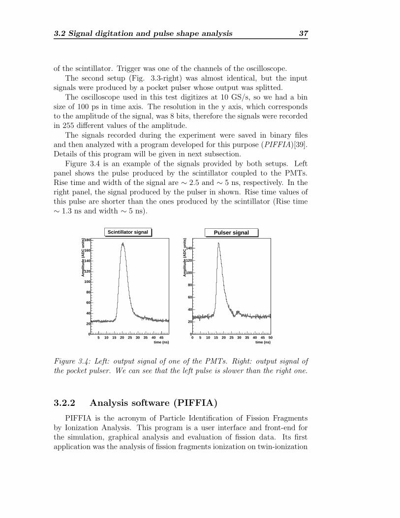
In order to investigate the time resolution that can be obtained by meansof a complete signal digitation method, we have used the setups shown inthe figure 3.3.

The first setup used in this experiment (Fig.3.3-left ) consisted on a BC420plastic scintillator (20 cm long, 4 cm high and 5 mm thick) coupled to twoHamamatsu 2431 photomultiplier tubes (PMT) placed at both sides of thescintillator. Neither light guides nor optical grease were used. In order tomeasure the time resolution, one of the outputs was delayed and both wereconnected to two of the channels of a digital oscilloscope (Tektronix TDS-7404) [38], thus we had two values for the time and the possibility to measureleft-right time difference.

The plastic was excited with a UV laser always impinging at the centerPSfrag replacements

TEKTRONIX TDS-7404 TEKTRONIX TDS-7404

PMT PMTScint.Pocket Pulser

16 Ω

Figure 3.3: Experimental setups used for the acquisition of signals and pulseshape analysis.


of the scintillator. Trigger was one of the channels of the oscilloscope.The second setup (Fig. 3.3-right) was almost identical, but the input

signals were produced by a pocket pulser whose output was splitted.The oscilloscope used in this test digitizes at 10 GS/s, so we had a bin

size of 100 ps in time axis. The resolution in the y axis, which correspondsto the amplitude of the signal, was 8 bits, therefore the signals were recordedin 255 different values of the amplitude.

The signals recorded during the experiment were saved in binary filesand then analyzed with a program developed for this purpose (PIFFIA)[39].Details of this program will be given in next subsection.

Figure 3.4 is an example of the signals provided by both setups. Leftpanel shows the pulse produced by the scintillator coupled to the PMTs.Rise time and width of the signal are ∼ 2.5 and ∼ 5 ns, respectively. In theright panel, the signal produced by the pulser in shown. Rise time values ofthis pulse are shorter than the ones produced by the scintillator (Rise time∼ 1.3 ns and width ∼ 5 ns).

time (ns)5 10 15 20 25 30 35 40 45

Am

plit

ud

e (A

DC

un

its)

0

20

40

60

80

100

120

140

160

180

Scintillator signal

time (ns)0 5 10 15 20 25 30 35 40 45 50

Am

plit

ud

e (A

DC

un

its)

0

20

40

60

80

100

120

140

Pulser signal

Figure 3.4: Left: output signal of one of the PMTs. Right: output signal ofthe pocket pulser. We can see that the left pulse is slower than the right one.

3.2.2 Analysis software (PIFFIA)

PIFFIA is the acronym of Particle Identification of Fission Fragmentsby Ionization Analysis. This program is a user interface and front-end forthe simulation, graphical analysis and evaluation of fission data. Its firstapplication was the analysis of fission fragments ionization on twin-ionization


chambers. Due to the modularization of the code, PIFFIA allows the use ofalternative algorythms. PIFFIA code is written in C++, an Object Orientedprogramming language, and uses all the power of the ROOT framework forhistogramming, curve fitting and graphical visualization [40].

Like most of the software developed in C++, PIFFIA is constituted by aset of classes. There is a manager class, Piffia, which controls the event loopfor the event readout and analysis. Another important class is PiffiaConfig,a configuration class which allows the user to control the values of all theconfiguration parameters, such as fitting intervals, thesholds, etc.. As faras our analysis is concerned, there are two important classes. The first onedefines all the parameters which characterise the signal,(PiffiaSignalObs)such as maximum voltage of the signal, etc. The second one calculates theparameters defined in the first class (PiffiaObsAnal).

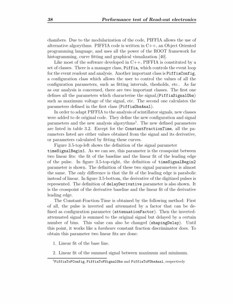
In order to adapt PIFFIA to the analysis of scintillator signals, new classeswere added to de original code. They define the new configuration and signalparameters and the new analysis algorythms1. The new defined parametersare listed in table 3.2. Except for the ConstantFractionTime, all the pa-rameters listed are either values obtained from the signal and its derivative,or parameters calculated by fitting these curves.

Figure 3.5-top-left shows the definition of the signal parametertimeSignalBegin1. As we can see, this parameter is the crosspoint betweentwo linear fits: the fit of the baseline and the linear fit of the leading edgeof the pulse. In figure 3.5-top-right, the definition of timeSignalBegin2

parameter is shown. The definition of these two signal parameters is almostthe same. The only difference is that the fit of the leading edge is parabolicinstead of linear. In figure 3.5-bottom, the derivative of the digitized pulses isrepresented. The definition of delayDerivative parameter is also shown. Itis the crosspoint of the derivative baseline and the linear fit of the derivativeleading edge.

The Constant-Fraction-Time is obtained by the following method: Firstof all, the pulse is inverted and attenuated by a factor that can be de-fined as configuration parameter (attenuationFactor). Then the inverted-attenuated signal is summed to the original signal but delayed by a certainnumber of bins. This value can also be changed (shapingDelay). Untilthis point, it works like a hardware constant fraction discriminator does. Toobtain this parameter two linear fits are done:

1. Linear fit of the base line.

2. Linear fit of the summed signal between maximum and minimum.

1PiffiaToFConfig, PiffiaToFSignalObs and PiffiaToFObsAnal, respectively


time (ns)10 15 20 25 30 35 40 45

Am

plit

ud

e (A

DC

un

its)

0

20

40

60

80

100

120

140

160

180

signal

timeSignalBegin1

timePeakVoltage

time (ns)10 15 20 25 30 35 40 45

Am

plit

ud

e (A

DC

un

its)

0

20

40

60

80

100

120

140

160

180

signal

timeSignalBegin2

time (ns)10 15 20 25 30 35 40 45 50

-15000

-10000

-5000

0

5000

10000

15000

20000

Derivative

delayDerivative

timeMaxDerivative

Figure 3.5: Definition of some signal parameters.

The ConstantFractionTime will be given by the crossing point of bothlinear fits (See figure 3.6).

There is another class which stores each pair of left-right signals param-eters and has the definition of all the ways of computing time:(PiffiaToFPairObs). The time is obtained by the following method:

Once all the parameters listed in table 3.2 have been calculated, theyare stored in different branches depending on whether they are Left or Rightevents. The ways of computing the time is the following:

• The left-light difference is calculated for each of the time parametersdefined (timePeakVoltage, timeSignalBegin1, timesignalBegin2, etc).Based on the parameter timeAtXPercent, a new time parameter isdefined. This is the so-called Double discrimination. It consists onobtaining the crossing point of the baseline and the line which joins thetwo points where two fractions of the maximum voltage are reached inthe leading edge. For instance Double Discrimination (20% 60%) isthe crossing point of the baseline and the line that joins the points0.2 × Amplitude and 0.6 × Amplitude in the leading edge of pulse.


Name Description

Amplitude Value of the maximum voltage of the signal(in ADC units).

timePeakVoltage Time of the maximum voltage of the signal.

timeSignalBegin1 Crosspoint of the linear fit of the leading edgeof the signal and the base line.

timeSignalBegin2 The same as timeSignalBegin1, but the fit isparabolic.

max(min)Derivative Maximum (minimum) value of the deriva-tive.

delayDerivative The same as timeSignalBegin1, but for thederivative.

timeAtXPercent Time at diferent percentages of the maxi-mum voltage (X= 20, 40, 60, 80).

timeAtFixedThreshold Time when the signal reaches a determinedvalue.

ConstantFractionTime Contant Fraction time by software (See textfor details).

Table 3.2: Description of the different parameters used for the characteriza-tion of the signal. The names correspond with the ones used in the PIFFIAprogram.

Operation of PIFFIA

1. Data acquired with the oscilloscope are readout sequentially from bi-nary files.

2. Signals are analyzed in an event-by-event basis to determine the pa-rameters. Several checks on the signal quality are also performed.

3. The value of all parameters characterising a signal are stored in differentleaves of a ROOT Tree in order to be able to access to each one easily,e.g., with a ROOT Browser.

In order to obtain the time resolution asociated with the different param-eters used to define the time, their respective values are stored in histograms.


time (ns)0 5 10 15 20 25 30

Am

plit

ud

e (A

DC

un

its)

-20

0

20

40

60

80

100

120

Constant Fraction Signal

Constant Fraction

time

Figure 3.6: Constant fraction signal and details of the calculation of theobservable ConstantFractionTime. Horizontal Line: Linear fit of base line.The other line is a linear fit of the signal between the maximum and minimumof the signal.

The resolution will be given by the width of the gaussian fit of the sistributionof these histograms.

3.2.3 Results

The results obtained from the analysis of the signals recorded with theexperimental setup described in section 3.2.1 are presented in this subsection.

Pocket pulser

The analysis of the signals produced by the pocket pulser makes possibleto obtain the contibution to total time resolution due to the readout andpulse shape analysis method.

Figure 3.7 shows the distributions of some of the parameters calculated.These distributions have been obtained from the analysis of 14000 signalsproduced by the pocket pulser. As we can see, in some of them it is possibleto distinguish two peaks corresponding to the left and right channels(bottom-left and right panels). The narrowest distributions are obtained for theparabolic fit of the leading edge of the pulse (bottom-left) and the constantfraction (bottom-right). In figure 3.8, we show the histograms obtained forthe left-right time differences.


time (ns)16 16.2 16.4 16.6 16.8 17

Co

un

ts

0

200

400

600

800

1000

Time Peak Voltage

time (ns)13 13.2 13.4 13.6 13.8 14 14.2

Co

un

ts

0

200

400

600

800

1000

Time at 5%

time (ns)14.2 14.3 14.4 14.5 14.6 14.7

Co

un

ts

0

500

1000

1500

2000

2500

3000

Parabolic fit leading edge

time (ns)16.8 16.85 16.9 16.95 17 17.05 17.1 17.15 17.2 17.25

Co

un

ts

0200400600800

1000120014001600180020002200

Constant Fraction

Figure 3.7: Distributions of different pulse parameters for 14000 events withthe pocket pulser. Top-left: Distribution of time when the peak voltage isreached. Top-right: Time at 5 per cent of the peak voltage. Bottom-left:Histogram representing the distribution of the observable timeSignalBegin2defined in table 3.2. Bottom-right: Distribution of constant fraction time for0.4 attenuation factor and 208 bins of shaping delay. We can see they havethe narrowest peaks.

Table 3.3 presents the time resolution achieved for each of the parametersdefined to characterise the signal. As we can see, depending on the parameter,the time resolution achieved ranges from 150 ps (σ) of the Peak Voltage tothe 9.6 ps of the constant fraction. We also see that for a fixed percentage ofthe signal, there is an optimium range between 40 and 60 percent of the peak,where the resolution is lower than 30 ps. Double discrimination presents itsbest value in 40%-80% (σ ≈ 30 ps).

For the derivative of the signal, obtained with the following relation:

Der =A(t + ∆t) − A(t)

∆t=

∆A

∆t(3.1)

where A is the amplitude of the signal, the distributions of the observablesare wider than the signal itself (Fig. 3.9) . This could be due to the number


/ ndf 2χ 2155 / 87

Constant 4.4± 383.2

Mean 0.0014± 0.3565

Sigma 0.0011± 0.1481

time (ns)-0.2 0 0.2 0.4 0.6 0.8 1

Co

un

ts

0

200

400

600

800

1000 / ndf 2χ 2155 / 87


Mean 0.0014± 0.3565

Sigma 0.0011± 0.1481

/ ndf 2χ 8926 / 67


Mean 0.0006± 0.3409

Sigma 0.00037± 0.03147

time (ns)0.1 0.15 0.2 0.25 0.3 0.35 0.4 0.45 0.5 0.55 0.6

Co

un

ts

0

200

400

600

800

1000

1200

/ ndf 2χ 8926 / 67


Mean 0.0006± 0.3409

Sigma 0.00037± 0.03147

/ ndf 2χ 3850 / 66


Mean 0.000± 0.344

Sigma 0.00025± 0.03532

time (ns)0.2 0.25 0.3 0.35 0.4 0.45 0.5

Co

un

ts

0

100

200

300

400

500

600

700

800

/ ndf 2χ 3850 / 66


Mean 0.000± 0.344

Sigma 0.00025± 0.03532

/ ndf 2χ 3368 / 58


Mean 0.0003± 0.3444

Sigma 0.00023± 0.03095

time (ns)0.2 0.25 0.3 0.35 0.4 0.45 0.5

Co

un

ts

0100200300400500600700800900

/ ndf 2χ 3368 / 58


Mean 0.0003± 0.3444

Sigma 0.00023± 0.03095

/ ndf 2χ 30.25 / 48


Mean 0.0001± 0.4249

Sigma 0.00008± 0.01311

time (ns)0.34 0.36 0.38 0.4 0.42 0.44 0.46 0.48 0.5

Co

un

ts

0

100

200

300

400

500

600

700

800

/ ndf 2χ 30.25 / 48


Mean 0.0001± 0.4249

Sigma 0.00008± 0.01311

/ ndf 2χ 286 / 74


Mean 0.0001± 0.2969

Sigma 0.000062± 0.009548

time (ns)0.25 0.26 0.27 0.28 0.29 0.3 0.31 0.32 0.33 0.34 0.35

Co

un

ts

0

100

200

300

400

500

600 / ndf 2χ 286 / 74


Mean 0.0001± 0.2969

Sigma 0.000062± 0.009548

Figure 3.8: Histograms representing the distributions of the time differencesfor different observables calculated with PIFFIA. Top panels: Left: time at5% of the peak voltage. Right: time at 20 %. Middle panels: Left: Dou-ble Discrimination (20%-80%). Right: Double Discrimination (20%-60%).Bottom panels: Left: Parabolic fit of leading edge. Right: Constant Fraction.Resolution is given by the σ of the distributions’ gaussian fits. The best resultis the one obtained for the constant fraction σ = 9.6 ps (bottom-right).

of bins, which is not enough for making a good fit of the leading edge for thederivative. The reason for this is that the precision in A is only one bit, butfor the time is 10−2, so the precision for the derivative is

σDer

Der=

√

(σ∆A

∆A

)2

+(σ∆t

∆t

)2

(3.2)

and, if the resolution in the time is much bigger than the resolution of theamplitude, the precision in the derivative is almost the same than ampli-tude’s.


time (ns)

12.8 13 13.2 13.4 13.6 13.8 14

Coun

ts

0

200

400

600

800

1000

1200

1400

1600

/ ndf 2χ 85.89 / 71


Mean 0.0008± 0.5899

Sigma 0.00056± 0.09006

time (ns)

0 0.1 0.2 0.3 0.4 0.5 0.6 0.7 0.8 0.9 1

Coun

ts

0

100

200

300

400

500

600

/ ndf 2χ 85.89 / 71


Mean 0.0008± 0.5899

Sigma 0.00056± 0.09006

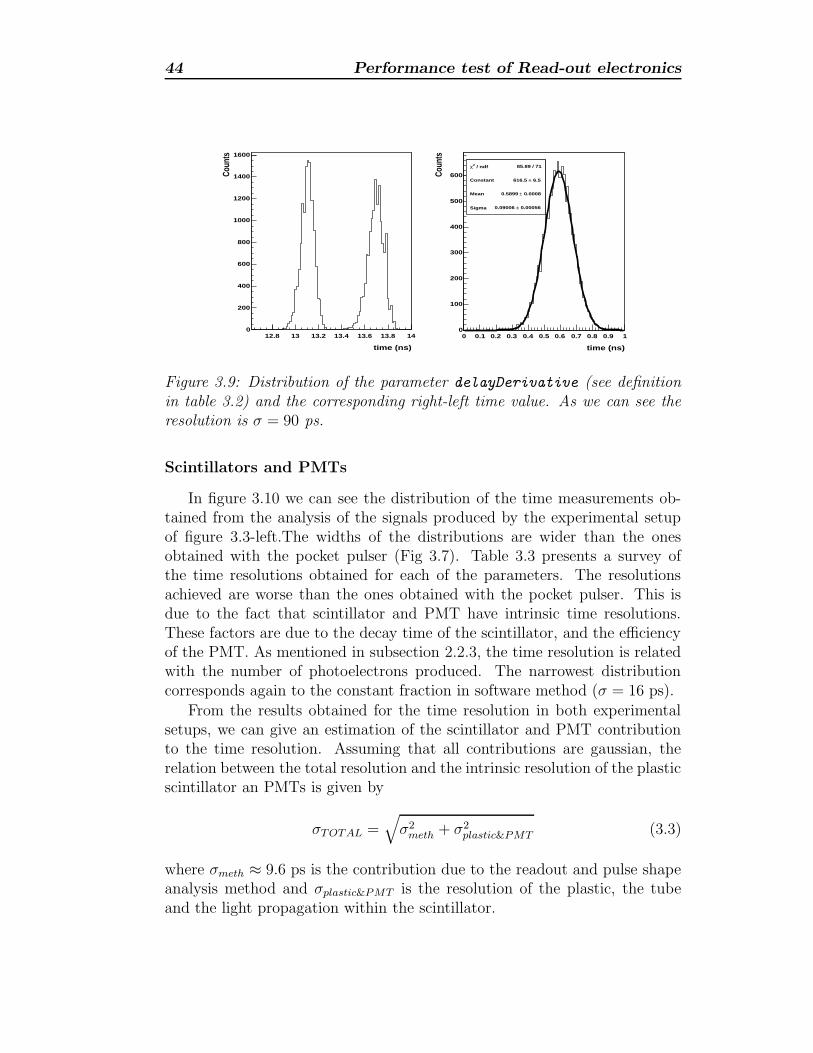
Figure 3.9: Distribution of the parameter delayDerivative (see definitionin table 3.2) and the corresponding right-left time value. As we can see theresolution is σ = 90 ps.

Scintillators and PMTs

In figure 3.10 we can see the distribution of the time measurements ob-tained from the analysis of the signals produced by the experimental setupof figure 3.3-left.The widths of the distributions are wider than the onesobtained with the pocket pulser (Fig 3.7). Table 3.3 presents a survey ofthe time resolutions obtained for each of the parameters. The resolutionsachieved are worse than the ones obtained with the pocket pulser. This isdue to the fact that scintillator and PMT have intrinsic time resolutions.These factors are due to the decay time of the scintillator, and the efficiencyof the PMT. As mentioned in subsection 2.2.3, the time resolution is relatedwith the number of photoelectrons produced. The narrowest distributioncorresponds again to the constant fraction in software method (σ = 16 ps).

From the results obtained for the time resolution in both experimentalsetups, we can give an estimation of the scintillator and PMT contributionto the time resolution. Assuming that all contributions are gaussian, therelation between the total resolution and the intrinsic resolution of the plasticscintillator an PMTs is given by

σTOTAL =√

σ2

meth + σ2

plastic&PMT (3.3)

where σmeth ≈ 9.6 ps is the contribution due to the readout and pulse shapeanalysis method and σplastic&PMT is the resolution of the plastic, the tubeand the light propagation within the scintillator.


Parameter Time Resolution (ps)

Pulser Scintillator

ConstantFractionTime 9.6 16.0

DoubleDiscriminator(20%-60%) 30.9 36.1



DelayDerivative 90.1 150.0

TimeAtFixedThreshold 50.4 60.2

Timeat20Percent 31.5 36.4




timePeakVoltage 155.0 313.0

timeSignalBegin2 13.1 18.3

timeSignalBegin1 25.9 29.7

Table 3.3: Time resolutions obtained for the parameters used for the charac-terization of the signal.

From equation (3.3) and the results obtained for the time resolution withthe constant fraction method, we can estimate σplastic&PMT to be around 12.8ps. The difference between this value and the one obtained with modularelectronics might be due to the resolution in amplitude of the oscilloscopeIt should be taken into account that these results have been obtained byimpinging the UV laser always at the same point of the scintillator, thereforethis resolution is dominated by the statistical nature of the scintillation andthe response of the PMTs.

In order to obtain more realistic results of the time resolution which can beachieved by pulse shape analysis some signals obtained with particle beamsor cosmic rays should be analyzed using this method.


/ ndf 2χ 195.6 / 76


Mean 0.003± 0.334

Sigma 0.00267± 0.08254

time (ns)0 0.1 0.2 0.3 0.4 0.5 0.6

Co

un

ts

0

10

20

30

40

50

60

70

80

90 / ndf 2χ 195.6 / 76


Mean 0.003± 0.334

Sigma 0.00267± 0.08254

/ ndf 2χ 131 / 57


Mean 0.0013± 0.4071

Sigma 0.00117± 0.03639

time (ns)0.25 0.3 0.35 0.4 0.45 0.5 0.55 0.6 0.65

Co

un

ts

0

10

20

30

40

50

60

70

80 / ndf 2χ 131 / 57


Mean 0.0013± 0.4071

Sigma 0.00117± 0.03639

/ ndf 2χ 55.35 / 62


Mean 0.0013± 0.4942

Sigma 0.00104± 0.03785

time (ns)0.3 0.35 0.4 0.45 0.5 0.55 0.6 0.65

Co

un

ts

05

1015202530354045

/ ndf 2χ 55.35 / 62


Mean 0.0013± 0.4942

Sigma 0.00104± 0.03785

/ ndf 2χ 46.06 / 51


Mean 0.0011± 0.4845

Sigma 0.00105± 0.03178

time (ns)0.3 0.35 0.4 0.45 0.5 0.55 0.6 0.65

Co

un

ts

0

10

20

30

40

50

/ ndf 2χ 46.06 / 51


Mean 0.0011± 0.4845

Sigma 0.00105± 0.03178

/ ndf 2χ 61.9 / 70

Constant 1.09± 25.22 Mean 0.0005± 0.4121

Sigma 0.0004± 0.0137

time (ns)0.37 0.38 0.39 0.4 0.41 0.42 0.43 0.44 0.45

Co

un

ts

0

5

10

15

20

25

30

35 / ndf 2χ 61.9 / 70

Constant 1.09± 25.22 Mean 0.0005± 0.4121

Sigma 0.0004± 0.0137

/ ndf 2χ 62.02 / 52


Mean 0.0006± 0.4752

Sigma 0.00051± 0.01603

time (ns)0.42 0.44 0.46 0.48 0.5 0.52 0.54

Co

un

ts

0

10

20

30

40

50 / ndf 2χ 62.02 / 52


Mean 0.0006± 0.4752

Sigma 0.00051± 0.01603

Figure 3.10: Time distributions of parameters shown in Fig. 3.8 for scin-tillator and PMT signals. As we can see the distributions are wider thanthe ones obtained with the pulser. The narrowest one is again for the onecorresponding to the constant fraction (σ ≈ 16 ps.)

3.3 FEE+TAQUILA digitation card 47

3.3 Integrated electronics:FEE+ TAQUILA

digitation card

Another possibility for the data readout is the use of standard electronics.In particular, in this work we have checked the time performances of theFront End Electronics (FEE) and TAQUILA digitation card developed bythe electronics department at GSI for the FOPI experiment [2]. It consistson a 16 channel FEE card with a gain of α ∼ 200 and a bandwidth ofδf ∼ 1000 MHz. This FEE card has a single ended 50 Ω input and twodifferencial outputs per channel for timing and charge. The amplification isdone in three stages. The discrimination of the timing signals is also done inthis card.

The FEE card is directly connected to the digitation card (TAQUILA)[2], which contains a 16 channel Time to Amplitude Converter (TAC) system.This TAC is operated in common stop mode: Each signal starts its individualTAC which is then stopped by the next cycle of a 40 MHz master clock (Fig.3.11). The total charge of the signal is digitized by a QDC. Figure 3.12 showsa picture of the FEE and the TAQUILA digitation card.

PSfrag replacements

time

START

STOPTAC

40 MHz clock

Figure 3.11: Operation of the TAC in common stop mode.


In order to determine the time resolution that can be achieved with thisnew electronics and check whether it is appropriate for our time-of-flightmeasurements, we have made a test of its performance. The setup used forthe test is described in the following.

The input signal was produced by an ORTEC 462 time calibrator [36](Amplitude ∼ 230 mV, risetime 1.5 ns.). This signal was splitted and sent totwo different channels of the FEE card. The output signals of the TAQUILA


Figure 3.12: The FEE and TAQUILA card

were sent via a GTB bus to a SAM3 VME module [41]. This module wasused as readout processor. The acqisition was controlled by the GSI MBSacquisition system. Figure 3.13 shows a diagram of the setup for one of thechannels. The information on the charge and time for both channels wassaved in a binary file.

PSfrag replacements

Time Calibrator

16 Ω

VME

RIO 3 CPU

Fan Out

Fan Out

Trigger Module

Gate Generator

Gate Generator

Constant Fraction

FEE+TAQUILA

FEE Input

SAM 3

OVL

Total Dead Time

A

B

C

Figure 3.13: Block diagram of the setup and the acquisition system. Theupper part corresponds to the gate generators for the acquisition.

3.3 FEE+TAQUILA digitation card 49

3.3.2 Results

Figure 3.14 shows the distributions of TAC values for the two channelsevaluated in this test. The distributions are almost uniform, except for thefirst values where we can observe a peak in both channels. This might be dueto inestabilities of the electronics for very short time differences, and affectsonly to a small time interval (∼ 200 ps). Even making a cut fo events withtime value lower than 300 ps, the number of events lost is less than a 0.5%of the total events. There is a small delay between both distributions. Thisfact is due to the different lengths of the cables from the signal splitter. Thevalue of the delay can be directly measured in the histograms, and is around2 channels.

TAC value (ADC units)1000 1500 2000 2500 3000

Co

un

ts

0

2000

4000

6000

8000

10000

12000

14000

16000

TAC distribution Channel 1

TAC value (ADC units)1000 1500 2000 2500 3000

Co

un

ts

0

2000

4000

6000

8000

10000

12000

14000

16000

18000

TAC distribution Channel 2

Figure 3.14: Distribution of TAC values for both channels.

For the calibration of the TAC values, we used the fact that the stop iscontrolled by the 40 MHz clock, therefore, the maximum TAC value corre-sponds to 25 ns. By counting the number of ADC channels, we can estimatethe calibration factors for each channel (Tab. 3.4).

In order to obtain the intrinsic resolution of this electronics, we calculatethe difference between time values (TAC value×calibration factor) obtainedfor each channel (∆T = T1 − T2). This values have been obtained by usingthe callibration factors of table 3.4.

Figure 3.15-top shows the stability of the time difference versus the clock-ing cycle. As we can see, except for the first values, this value is almost con-


Channel nr. Nr. of bins Cal. factor(ps/bin)

1 2147 11.64

2 2176 11.48

Table 3.4: Calibration factors for both channels.

stant. Figure 3.15-bottom-left shows the projection of the time difference,in the interval 5-10 ns, before the correction. As we can see the value of thetime resolution, given by the width of the gaussian fit of this distribution isσ = 25.2 ps.

As shown in figure 3.15-top-right, the time difference between the chan-nels presents a slightly non-linear behaviour. This behaviour may be cor-rected by means of a polynomial fit. In order to correct this non linear-ity, these data have been fitted to a 6th degree polynomial function. Bysubstracting the fitted values to the original ones is possible to ’straightenup’ the distribution and improve the time resolution achieved. Figure 3.15-bottom-right presents the distribution of the corrected time difference, andthe time resolution is σ = 19.8 ps, therefore, this correction method improvesthe resolution by a 20%. Other intervals have been chacked obtaining similarresults (σ ≈ 20 ps).

3.4 Conclusions

In this chapter, we have presented the results obtained from the test ofthree different readout methods: standard modular electronics, pulse shapeanalysis and the new TAQUILA electronics.

The time resolution obtained with modular electronics is very good. In-trinsic electronics resolution is σelec ≈ 8 ps. and the intrinsic resolution ofplastic scintillator combined with the PMTs depends on two factors (see ta-ble 3.1), the high voltage applied and the intensity of the laser. Very highvoltages produce worse time resolution. This fact could be due to the appear-ance of noise in the photomultiplier. The second factor is related with thefact that time resolution in scintillation detector is related with the numberof photoelectrons, as shown in section 2.2.3. The intrinsic time resolutionmeasured is around σ ∼ 8 ps.

Results obtained with pulse shape analysis have shown that the timeresolution depends on the choice of the signal parameter which defines thetime value, ranging from 300 to 16 ps. The best result obtained in this case

3.4 Conclusions 51

Figure 3.15: Top: Stability of the time difference of the TAQUILA+FEEsystem versus the clocking cycle. right panel is a zoom of this distribution.We can see the slightly non-linear behaviour. Bottom-left: Projected time dif-ference between both channels between 5 and 10 ns. Bottom-right: Projectedtime difference after correction in the same range. The width of the gaussianfit gives the time resolution.

corresponds to the implementation of a constant fraction in software (σ < 10ps). The resolution of the method is σ = 9.6 ps, thus the intrinsic timeresolution obtained for the plastic and PMT is ≈ 12.8 ps. The differencebetween this result and the results achieved with modular electronics (σ ≈ 8ps) might be due to different high voltages applied in the phototubes ordifferent intensities of the laser used, as well as the amplitude resolution ofthe oscilloscope. This method is therefore very appropriate to achieve thetime resolutions required.

From these two methods, we can estimate that the intrinsic time resolu-tion of scintillators and PMTs is around 10 ps (σ).

It should be taken into account the fact that these data correspond to aUV laser and a relatively small scintillator, so all the pulses have the same


amplitude and shape. In order to obtain more realistic results, some testswith particle beams or cosmic rays should be performed.

One of the main drawbacks of this readout method is the very high costper channel. This readout is only affordable for systems with a relativelysmall number of channels.

Results obtained with the TAQUILA card, are very good (σ ≈ 20 ps).They are not as good as the best resolution obtained from pulse shape anal-ysis. The main advantage of this readout method is that it is much cheaper,and therefore, more appropriate for detectors with a large number of elec-tronic channels. Comparing this time resolution with the ones achieved withother read-out RPC electronics, such as the one developed for ALICE exper-iment, this values are better than the the resolution measured (σTDC = 20ps [31] and σFEE&cables ∼ 12 ps), although ALICE results correspond to areal test with the beam). In our case, we have only tested two channels witha time calibrator. These results obtained have shown that this electronics issuitable for our high resolution time measurements. Again, this test allowsonly to obtain the intrinsic resolution of the electronics. If we want to mea-sure the time resolution which can be achieved, a test beam with detectorsshould be performed, but the results obtained are very encouraging.

Chapter 4

Conceptual Design

In this chapter, the design of a high resolution time-of-flight wall forcharged particles and ions is proposed as a part of the R3B detection system.

According with the requirements discussed in section 1.3, we present twopossible alternatives for the construction of the ToF wall: Resistive PlateChambers (RPCs) and Scintillators coupled to fast photomultiplier tubes.

4.1 Design concepts

4.1.1 RPCs

As mentioned in chapter 2, RPCs have been used to construct large areatime of flight detectors, reaching time resolutions of the order of σToF < 60ps. However, most of the designed RPCs are used with minimum ionizingparticles [2, 27, 28], and very little information is avaliable about the responseof these detectors with heavy ions [29].

Geometry

The design of a large area ToF wall made of three detection planes rotated120 one respect to the other is proposed (Fig. 4.1-left). Each plane willconsist on 8 modules according to the geometry shown in figure 4.1-right.There are 6 horizontal modules and the last two are placed vertically inorder to cover the 1.5 m diameter surface corresponding to the acceptanceof fission fragments flying at 600 MeV/u (Sect. 1.3.3). The surface coveredby the three detection planes is higher than 99% of full acceptance for 600MeV/u beams (Fig. 4.2). Every plane presents a segmented readout systemin order to determine the position.

54 Conceptual Design

Figure 4.1: Schematic representation of the design proposed for the ToF wall.The left panel shows the three detection planes. The right panel representsthe proposed geometry for the 8 RPC modules that constitute each plane.

(MeV/u)E200 300 400 500 600 700 800 900 1000 1100

Acc

epta

nce

(%

)

50

60

70

80

90

100

Angular acceptance VS beam energy

Figure 4.2: Angular acceptance of the RPC wall coverd by the three detectionplanes for different energies of the beam. The full acceptance is achieved forenergies larger than 600 MeV/u.

This multilayer design allows also to reduce the obtained time resolu-tion with a single layer detector by a factor

√3, provided that particle has

produced signals in all the layers. Assuming a time resolution of 50 ps (σ)per plane, the resulting time resolution expected is therefore of the order ofσToF = 50/

√3 ≈ 30 ps.

4.1 Design concepts 55

RPC modules

As mentioned before, each detection plane will be constituted by eightmodules. Every module would be a 2-gap resistive plate chamber with adimension of 100×26 cm2. In principle, a stack of three glass plates (2 mmthick each) is considered, spaced one from the other with nylon fishing linewith a diameter of 300 µm, creating two different gas gaps. The gas gaps willbe filled with the standard mixture (see section 2.1.2). The outer surfaces ofthe two outer glass plates will be in contact with a conductive layer acting aselectrodes (graphite or nickel paint have been considered). A differential highvoltage to produce an electric field of typically 100 kV/cm will be appliedto the electrodes. Then a mylar or kapton foil will isolate them from thereadout system. This system consists on two printed circuit board plates(around 2 mm thick) surrounding the stack of glass plates. These plates willhave copper pick-up strips in the inner surfaces. The PCB plates, will alsoconstitute the main frame of each RPC module. A cross section of the designis shown in figure 4.3.

PSfrag replacements

2 mm PCB

100 µm Cu

50 µm mylar,kapton

∼ 30 µm graphite, Ni paint

2 mm glass

Figure 4.3: A cross section (not to scale) of one RPC module is shown withthe three inner glass plates surrounded by the electrodes, the mylar foils andthe PCB plates with the copper strips acting as signal pick up system.

Energy losses per detector module have been calculated using AMADEUSfor different charges and energies of the fragments as well as energy depositedin the gas gaps in order to evaluate the minimum energy and charge thatwill be detected by the ToF wall (See figure 4.4). From the results obtained,we can conclude that fragments heavier than 208Pb at energies around 500MeV/u will not traverse all the planes of the ToF wall at energies around andbelow 500 MeV/u. Lighter elements will traverse all the detection planes,and the energy deposited in gas will be of the order of MeV, except for those


lighter than 12C. The energy deposited in the gas by this fragments is somekeV, therefore is is enough to produce ionizations in gas.

Atomic Number10 20 30 40 50 60 70 80 90 100

(MeV

)ga

p E∆

0

5

10

15

20

25

30 Gap 1Gap 2Gap 3Gap 4Gap 5Gap 6

500 MeV/u

Atomic Number10 20 30 40 50 60 70 80 90 100

(MeV

)ga

p E∆

0

10

20

30

40

50


600 MeV/u

Atomic Number10 20 30 40 50 60 70 80 90 100

(MeV

)ga

p E∆

0

5

10

15

20

25

30


700 MeV/u

Figure 4.4: Energy deposited per gas gap in the ToF wall for different chargesand energies of the beam. Elements heavier than 208Pb at 500 MeV/u willnot traverse all the planes (top panel).

4.1 Design concepts 57

Readout system and electronics

At the moment we are considering the segmentation within each modulewith 10 copper strips per module (100 × 2.5 cm2) with 1 mm gap betweenthem. Anode and cathode strips will provide a differential signal. The signalsinduced by charged particles will be taken from both sides of the RPC mod-ule, determining the position along the 1 m length with a resolution betterthan 3 mm (see sect. 1.4). This segmented readout strips configuration pro-vides individual detection cells with a surface of about 12 cm2 (Fig. 4.5-left),minimizing the multihit probability. The probability of multihit is bellow1% for fission fragments at 600 MeV/u and better than 7% even for multi-fragmentation reactions (5 fragments). The position information would alsohelp to correct the time of flight with a better definition of the pathlength,improving the final time resolution. In order to reduce the number of elec-tronic channels without losing resolution in position, the signals induced intwo consecutive strips could be read by the same amplifier and disentangledlater by comparing both sides of the fired strips (Fig. 4.5-right).

PSfrag replacements

OUT

OUT

Figure 4.5: Left: Front view of the ToF wall detector with individual detectioncells defined by the geometry of the pickup strips. Right: Readout scheme ofthe pickup strips.

For the read-out electronics the TAQUILA [2] front end electronics andreadout system is considered. This electronics allows the measurement oftime and charge of the signals induced in the pickup electrodes. The intrinsicresolution of this electronics is around 20 ps, fulfilling our requirements (seesection 3.3 for details).


4.1.2 Plastic scintillators

As an alternative, we propose a ToF wall based in the use of standard or-ganic scintillators coupled to fast photomultipliers (PMT). In order to achievea time resolution below 60 ps we consider individual counters made of organicscintillator material with a dimension of 6×150 cm2 and a thickness of 5 mm.With this dimensions we will need 30 paddles with 1 cm overlap to cover the1.5 m2 total surface. As in the RPC design we will have multiple layers (twoinstead of three) disposed in a perpendicular configuration, being a totalnumber of 60 paddles (Fig. 4.6). These scintillator paddles will be equippedwith 120 light guides, photomultipliers and electronic channels. The accep-tance of this design is almost 100% for energies higher than 600 MeV/u,and the multihit probability considering 36 cm2 individual detection cells islower than 1% for fission fragments and around 14% in multifragmentationreactions (5 fragments).

!!!!!!!!!!!!

""""""""

######

$$$$$$

%%%%%%%%%

&&&&&&

''''''

((((((

)))))))))

******

++++++

,,,,,,

---------

......

////////

00000000

111111111111

22222222

33333333

44444444

555555555555

66666666

777777

888888

999999999

::::::

;;;;;;

<<<<<<

=========

>>>>>>

??????

@@@@@@

AAAAAAAAA

BBBBBB

CCCCCC

DDDDDD

EEEEEEEEE

FFFFFF

GGGGGG

HHHHHH

IIIIIIIII

JJJJJJ

KKKKKKKK

LLLLLLLL

MMMMMMMMMMMM

NNNNNNNN

OOOOOO

PPPPPP

QQQQQQQQQ

RRRRRR

SSSSSS

TTTTTT

UUUUUU

VVVVVV

WWWWWWWWW

XXXXXXYY

YYYY

ZZZZZZ

[[[[[[[[[

\\\\\\]]

]]]]

^^^^^^

_________

``````aa

aaaa

bbbbbb

ccccccccc

ddddddee

eeee

ffffff

ggggggggg

hhhhhhii

iiii

jjjjjj

kkkkkkkkk

llllllmm

mmmm

nnnnnn

ooooooooo

ppppppqq

qqqq

rrrrrr

sssssssss

tttttt

uuuuuu

vvvvvv

wwwwwwwww

xxxxxxyy

yyyy

zzzzzz

||||||

~~~~~~

¡¡¡¡¡¡¡¡¡

¢¢¢¢¢¢¢¢¢

£££££££££

¤¤¤¤¤¤¤¤¤

¥¥¥¥¥¥¥¥¥

¦¦¦¦¦¦

§§§§§§§§§

¨¨¨¨¨¨

©©©©©©

ªªªªªª

««««««

¬¬¬¬¬¬

®®®®®®

¯¯¯¯¯¯¯¯¯

°°°°°°°°°

±±±±±±±±±

²²²²²²²²²

³³³³³³³³³

´´´´´´´´´

µµµµµµµµµ

¶¶¶¶¶¶

·········

¸¸¸¸¸¸¸¸¸

¹¹¹¹¹¹¹¹¹

ººººººººº

»»»»»»»»»

¼¼¼¼¼¼

½½½½½½

¾¾¾¾¾¾

¿¿¿¿¿¿¿¿¿

ÀÀÀÀÀÀÀÀÀ

ÁÁÁÁÁÁÁÁÁ

ÂÂÂÂÂÂ

ÃÃÃÃÃÃ

ÄÄÄÄÄÄ

ÅÅÅÅÅÅÅÅÅ

ÆÆÆÆÆÆ

ÇÇÇÇÇÇ

ÈÈÈÈÈÈ

ÉÉÉÉÉÉÉÉÉ

ÊÊÊÊÊÊ

ËËËËËËËËË

ÌÌÌÌÌÌÌÌÌ

ÍÍÍÍÍÍÍÍÍ

ÎÎÎÎÎÎ

ÏÏÏÏÏÏ

ÐÐÐÐÐÐ

ÑÑÑÑÑÑ

ÒÒÒÒÒÒ

ÓÓÓÓÓÓ

ÔÔÔÔÔÔ

ÕÕÕÕÕÕ

ÖÖÖÖÖÖ

××××××

ØØØØØØ

Figure 4.6: Front view of the ToF wall detector based on scintillators.

Energy deposited in the scintillator material has also been calculated us-ing AMADEUS for different charges and energies of the fragments to evaluatethe minimum energy and charge that will be detected by the ToF wall (Seefigure 4.7). From these results, we see that all elements, from 12C to thoseheavier than 208Pb at energies around 500 MeV/u will traverse both planesof the ToF wall at energies around 500 MeV/u. The energy deposited inthe plastic by this fragments ranges from thousands to hundreds of MeV,

4.2 Cost estimate 59

Atomic Number10 20 30 40 50 60 70 80 90 100

E (

MeV

)∆

0

5000

10000

15000

20000

25000500 MeV/u

600 MeV/u

700 MeV/u

Energy loss in Scintillator

Figure 4.7: Front view of the ToF wall detector based on scintillators. Right:Readout scheme of the pickup strips.

therefore is enough to produce scintillation.As far as the time resolution is concerned, the total time resolution

achieved with this type of detectors is around 75 ps per layer for fission frag-ments [9]. Therefore the expected time resolution is around σToF = 75/

√2 ≈

53 ps.The use of Bicron BC420 as scintillation material coupled to Hamamatsu

H2431 tubes is considered. As in the RPC case, signals will be taken fromboth extremes of the scintillator. For the readout we propose the samesolution as for the RPC, although, in this case, the front end electronicsboard should be adapted to the PMT signals.

4.2 Cost estimate

In this section, the cost estimate of both designs proposed is presented.

4.2.1 RPCs

The cost estimate of such a ToF wall based on the concept describedabove is presented in table 4.1. This estimation was obtained assuming athree layer ToF wall made of eight RPC modules each, with 10 readout padsand collecting the signals from both extremes of the pads and reading thesignals of two consecutive strips with the same preamplifier. Then, 10 elec-tronic channels per module are needed, 80 channels per layer and a totalnumber of 243 channels. This number is due to the fact that readout strips


are connected according to figure 4.5-right. Housing and holding entry cor-responds to the design ans construction of a mechanical structure for thedetector. Gas system entry corresponds to the set of devices which allow tocontrol gas flow and mixture percentages in RPCs. Power supply is relatedwith the high voltage needed for the RPC to work. Cost estimation of it isbased on the price of standard high voltage power supplies. Electronics costestimate is based in the 200 euro per channel cost of the FEE+TAQUILA.DAQ entry corresponds to the data acquisition system. The accuracy in theestimation is of the order of 20 %.

Item cost (Keuro)

R&D+Prototypes 30

RPC materials 20

RPC housing & holding 30

Gas system 30

Power Supply 20

Electronics (243 ch.) 50

DAQ(SAM3+RIO3+crate) 35

Total 215

Table 4.1: Cost estimate for a three layer ToF wall based on RPCs

4.2.2 Plastic scintillators

The cost estimate for this option is presented in table 4.2. This estimationis based on the use of 30 horizontal and 30 vertical detectors equiped with120 PMTs and electronic channels. The estimation of the electronics cost isbased again in the use of FEE+TAQUILA option.

As we can see, the cost of an RPC based ToF wall versus a scintillatorbased one is a factor two cheaper. This is one of the reasons of using RPCsinstead of plastic scintillators. The cost is cheaper and the performances arealmost the same.

4.2 Cost estimate 61

Item cost (Keuro)

R&D+Prototypes 30

1.5×1.5 m2 BC420 10

Light guides 10

120 Hamamatsu 2431 PMTs 276

Mechanics 15

Power supply 50

Electronics (120 ch.) 24

DAQ(SAM3+RIO3+crate) 35

Total 450

Table 4.2: Cost estimate for a two layer ToF wall based on scintillators

Conclusions

The goal of this work was to define the performances of a ToF wall de-tector for heavy ion identification, discuss the present technologies avaliableto achieve these requirements and propose a conceptual design based on theprevious considerations.

This detector will be used to measure the time of flight in order to obtainthe velocities of the fragments coming out from the nuclear reactions inducedby relativistic heavy ions at the R3B experiment, that will take place at thenew FAIR facility in Darmstadt (Germany).

The main requirements are to cover the full acceptance of all the out-coming reaction products and to isotopically identify them up to the mass200. The possibility of multihit-event identification has also been consid-ered. According to this requirements the most appropriate features are thefollowing:

Tof resolution: The time accuracy needed to separate masses around A ∼200 at 700 MeV/u is around ∆ToF/ToF ≈7×10−4, for 15 m path-length this value σToF ≈ 20 ps, therefore this path-length seems rea-sonable for the nowadays timing technology.

Position and surface: As far as size is concerned, the one required to coverthe full acceptance for fission fragments at 500 MeV/u at 15 m formthe target is 1.5 × 1.5 m2.

Granularity: In order to make possible multi-hit event identification, thedetector will be divided in strips of 2.5 cm, providing a multihit prob-ability of double hits lower than 7% for multifragmentation reactions(5 fragments).

The START will be given by a CVD diamond detector.Due to the factthat diamond detectors’ intrinsic time resolution is σ = 29 ps, the resolutionwill be limited by this value. Other possible detectors should be consideredas START in order to avoid this limitation.

64 Conclusions

Two different technologies have been considered to implement such a de-tector: Resistive Plate Chambers (RPC), or fast plastic scintillators coupledto fast photomultiplier tubes.

Resistive Plate Chambers and scintillator detectors are very suitable de-vices for time-of-flight measurements. The efficiency and time resolutionachieved with the ‘state of the art’ timing RPCs, multigap glass RPCs ina range of 0.2-0.3 mm gap width, is about 99% and 50 ps (σ) respectivelyfor MIPS.Very little is known about the behaviour of RPCs with heavy ions.Further studies should be performed in order to check the performance ofRPCs with them, but these results are very encouraging for the use of thesetype of detectors in the identification of heavy ions by time of flight measure-ments, as an alternative to the standard scintillation detectors. Scintillatorshave shown excellent performances for new scintillation materials and photo-multiplier tecnologies (better than 10 ps (σ) for small scintillators and heavyions, around 75 ps(σ) for 1m scintillatos and fission fragments ).

Different readout methods for the signals have been tested: standardmodular electronics, pulse shape analysis and the new TAQUILA electronicsdeveloped for FOPI the RPCs.

The time resolution obtained with modular electronics is very good. Elec-tronics resolution is σelec ≈ 8 ps and the intrinsic resolution of plastic scin-tillator combined with the PMTs depends on two factors, the high voltageapplied and the light output, e.g. at very high voltages the time resolutiondeteriorates. The second factor is related with the fact that time resolutionin scintillation detectors improves with the number of photoelectrons. Frompulse shape analysis of the scintillators signals,we have shown that the timeresolution achievable depends on the parameter chosen to define the time,ranging from 300 to 16 ps. The best result obtained in this case correspondsto the implementation of a constant fraction in software. The intrinsic res-olution of the method has been measured with a pulser, obtaining σ = 9.6ps, thus the intrinsic time resolution of the plastic and PMT is ≈ 12.8 ps.The difference between this result and the results achieved with modularelectronics (σ ∼ 8 ps) might be due to different high voltages applied in thephototubes or different intensities of the laser used, as well as the amplituderesolution of the oscilloscope. This method is therefore very appropriate toachieve the time resolutions required.

It should be taken into account the fact that these data correspond to aUV laser and a relatively small scintillator, thus all the pulses have the sameamplitude and shape. In order to obtain more realistic results, some testswith particle beams or cosmic rays should be performed.

One of the main drawbacks of this readout method is the very high costper channel. This readout is only affordable for systems with a relatively

Conclusions 65

small number of channels.The results obtained with integrated electronics (TAQUILA card), are

very good (σ ≈ 20 ps). They are not as good as the best resolution obtainedfrom pulse shape analysis. The main advantage of this readout method isthat it is much cheaper, and therefore, more appropriate for detectors witha large number of electronic channels. The results obtained have shownthat this electronics is suitable for our high resolution time measurements.Comparing this time resolution with the one achieved with other read-outRPC electronics, such as the one developed for ALICE experiment, this val-ues are better than the the resolution measured (σTDC = 20 ps [31] andσFEE&cables ∼ 12 ps), although ALICE results correspond to a real test withthe beam). In our case, we have only tested two channels with a time cal-ibrator. Again, this test allows only to obtain the intrinsic resolution. Ifwe want to measure the real time resolution that can be achieved, a testbeam with detectors should be performed, but the results obtained are veryencouraging.

Finally, a large area ToF wall based on RPC detectors has been proposed.It consists on three detection planes rotated 120 one respect to the other.Each plane will consist on 8 modules. Every module will be a multigapresistive plate chamber with a dimension of 100 × 26 cm2 with a segmentedanode design. In principle, a stack of three gas plates is considered, spacedone from the other with nylon fishing line with a diameter of 300 µm, creatingtwo different gas gaps. The outer surfaces of the two outer glass plateswill be in contact with a conductive layer acting as electrodes (graphite ornickel paint have been considered). Then a mylar foil will isolate them. Thereadout system consist on two printed circuit board plates surrounding thestack of glass plates. These plates will have copper pick-up strips in the innersurfaces. At the moment we are considering 10 strips (100× 2.5 cm2) with 1mm gap between them, in order to pick up both anode and cathode signals.A differential high voltage will be applied to the electrodes. For the readout,a differential signal will be obtained from anode and cathode pick up strips.In order to reduce the number of electronic channels, the signals induced intwo consecutive strips could be read by the same amplifier, So the stripsizeis equivalent to a 5 cm one.

This design covers the required surface with 1.5 m diameter. In addition,it will allow to reduce the achievable time resolution with a single layerdetector by a factor

√3, resulting in a expected resolution of the order of

σToF = 30 ps. This configuration also provides individual detection cellswith a surface of about 12 cm2, minimizing the multihit probability. Thesignals induced by charged particles will be taken from both sides of the RPCmodule. These two measurements will allow to determine the position along

66 Conclusions

the 1 m length of the detector by the time difference method. In addition,this position information will help to correct the time-of-flight, improvingthe time resolution. For the read-out electronics the TAQUILA front endelectronics and readout system is considered.

Conclusiones

En este trabajo se ha pretendido definir los requisitos de un muro detectorde timepo de vuelo para la identificacion de iones pesados, discutir las dife-rentes tecnologıas disponibles actualmente para satisfacer estas necesidades,ası como proponer un diseno basado en las consideraciones anteriores.

Este detector se usara para la medida del tiempo de vuelo de los frag-mentos procedentes de las reacciones nucleares producidas por iones pesadosa energıas relativistas en el experimento R3B, que tendra lugar en la nuevasinstalaciones de FAIR en Darmstadt (Alemania).

Los requisitos principales que tiene que cumplir este detector son cubrirtoda la aceptancia de los productos de las reacciones y separarlos hastala masa 200. La posibilidad de identificar sucesos con impactos multiplestambien se ha tenido en cuenta, lo que va a determinar la granularidad denuestro detector. De acuerdo con estos requisitos, las caracterısticas masapropiadas son las siguientes:

Resolucion temporal: la resolucion necesaria para separar masas en tornoa A ∼ 200 a 700 MeV/u es aproximadamente ∆ToF/ToF ≈7×10−4,que para una distancia de 15 m entre los detectores se traduce en unaresolucion absoluta de σToF ≈ 20 ps. Por tanto, esta distancia parecerazonable dada la tecnologıa actual en cuestion de medida de timepos.

Posicion y superficie: en lo referente al tamano, el necesario para cubrirtoda la aceptancia de los fragmentos de fision a 500 MeV/u a una dis-tancia de 15 m desde el blanco es de 1,5 m de diametro. Debido ala fuerte focalizacion hadia adelante de los productos a energıas rela-tivistas, energıas mayores requieren una menor superficie, por lo que laaceptancia total esta garantizada para energıas superiores del haz.

Granularidad: Para posibilitar la identificacion de sucesos con impactosmultiples, el detectors debera estar dividido en tiras de 2,5 cm de ancho,proporcionando una probabilidad de impactos dobles inferior al 7%para reacciones en las que se han producido 5 fragmenos.

68 Conclusiones

El START vendra dado por un detector de diamante. Puesto que laresolucion temporal intrınseca de este tipo de detectores es σ = 29 ps, laresolucion total estara limitada por este valor, por tanto, se podrıa tener encuenta el uso de otro tipo de dispositivos para evitar esta limitacion. Parael STOP, se han considerado las dos tecnologıas mas utilizadas actualmentecamaras de placas resistivas (RPCs) y centelleadores rapidos acoplados a tu-bos fotomultiplicadores (PMTs) tambien rapidos. Ambos tipos de detectoresson adecuados para medidas de tiempo de vuelo de gran precision. La eficien-cia y la resolucion temporal alcanzadas actualmente con RPCs es del 99% y50 ps (σ), respectivamente con partıculas mınimamente ionizantes (MIPs).

Actualmente se sabe muy poco acerca del comportamiento de las RPCscon iones pesados y deberıan realizarse estudios para comprobar las presta-ciones de este tipo de detectores con ellos, como alternativa a los detectoresde centelleo usados normalmente.

El desarrollo de centelleadores rapidos junto con la evolucion de los fo-tomultiplicadores ha permitido alcanzar resoluciones temporales excelentes(menor de 10 ps (σ) para centelleadores pequenos y en torno a 75 ps(σ) paracentelleadores de 1 m y fragmentos de fision).

Para la lectura de las senales producidas por ambos tipos de detectores,se han probado tres metodos diferentes: la electronica modular utilizadanormalmente, la digitalizacion completa de las senales producidas para suposterior analisis mediante software y la tarjeta digitalizadora (TAQUILA)desarrollada para las RPCs del experimento FOPI.

La resolucion temporal ontenida con electronica modular es σelec ≈ 8 ps,mientras que la resolucion temporal de los centelleadores y los PMTs de-pende principalmente de dos factores: la tension aplicada y la luz producidaen el plastico. Por ejemplo, para voltajes muy altos en el PMT, la aparicionde ruıdo deteriora la resolucion temporal. La intensidad de la luz esta rela-cionada con el hecho de que en los detectores de centelleo, la resolucionmejora con el numero de fotoelectrones emitidos.

Del analisis del pulso digitalizado, se ha obtenido que la resolucion al-canzada depende del parametro escogido para definir el tiempo, y los val-ores varıan entre los 300 ps y los 16 ps (σ). Este ultimo resultado se haobtenido con la implementacion de un Constant Fraction Discriminator porsoftware. La resolucion intrınseca del metodo se ha medido con un gener-ador de pulsos y es σ ≈ 9.6 ps, por tanto la resolucion intrınseca del sis-tema plactico+PMT es σ ∼ 12, 8 ps. La diferencia entre este resultado y elobtenido con electronica modular (σ ∼ 8 ps) puede ser debida a que los volta-jes aplicados en los tubos o la intensidad del laser utilizado para excitar elplastico eran diferentes, ası como la resolucion en amplitud del osciloscopio.El uso de este metodo parece por tanto adecuado para obtener las resoluciones

Conclusiones 69

requeridas. Debe tenerse en cuenta el hecho de que los datos analizados cor-responden a un laser UV y a centelleadores relativamente pequenos. Comoconsecuencia, todos los pulsos tienen la misma forma y amplitud y la aten-uacion de la luz en el seno del centelleador no es significativa. Para obtenerresultados mas realistas, deberıan hacerse medidas con haces de partıculas orayos cosmicos.

Los resultados obtenidos con TAQUILA son muy buenos (σ ≈ 20 ps),aunque no tan buenos como los obtenidos por los dos metodos anteriores. Laventaja principal de este metodo es que es mucho mas barato, y por tantomas apropiado para detectores con varios cientos de canales de electronica.Los resultados obtenidos muestran que este tipo de electronica es adecuadapara nuestras medidas de tiempo. Comparando esta resolucion temporalcon la alcanzada por otras electronicas desarrolladas para RPCs, como porejemplo la de ALICE (σTDC = 20 ps y σFEE&cables ∼ 12 ps), los resultadosobtenidos con TAQUILA son mejores, aunque debe tenerse en cuenta quelos resultados de ALICE se corresponden con un test real, mientras que ennuestrocaso solo se han probado 2 canales con un calibrador de tiempos.

Finalmente, se ha propuesto el diseno de un muro de tiempo de vuelobasado en RPCs. Este muro esta formado por tres planos iguales rotados120 uno respecto de otro. Cada plano esta constituıdo por 8 modulos.Cada uno de los modulos es una RPC multigap de 100 × 26 cm2. Estediseno cubre la superficie requerida de 1.5 m de diametro con una aceptanciasuperior al 99% para la superficie comun a los tres planos. Ademas, permitereducir la resolucion temporal en un factor

√3 si se ha producido senal en

los tres planos, obteniento una resolucion temporal de σToF = 30 ps. Estaconfiguracion proporciona ademas celdas de deteccion con una superficiesde 15 cm2 aproximadamente, minimizando ası la probabilidad de impactosmultiples. La senal inducida en los electrodos de lectura es recogida a amboslados del modulo. Estas dos medidas permiten determinar la posicion a lolargo del modulo con una precision de aproximadamente 2 mm, podiendoası corregir la medida de tiempo de vuelo por la longitud recorrida. Para laelectronica de lectura se considera el uso de la TAQUILA.

Appendix A

Relation between resolution inbending angle and positionresolution of tracking detectors

We will derive here the expression which relates the resolution in themeasurement of the bending angle and the position resolution in trackingdetectors.

PSfrag replacements

`1 `2 `3

x1

x2

x3

xd

θ1

θ2

θ

Figure A.1: Relation between bending angle and position detectors.

72 Bending angle and position resolution

From Fig. A.1 the angles are defined as

θ2 ≈ tan θ2 =x3 − x2

`3

=x2 − xd

`2

(A.1)

θ1 ≈ xd − x1

`1

(A.2)

θ = θ2 − θ1 (A.3)

From eq. (A.1) we getxd = x2 − `2θ2 (A.4)

Using this result in eq. (A.2) and substituting in (A.3) we obtain

θ = θ2 −x2 − `2θ2 − x1

`1

=

(

1 +`2

`1

)

θ2 −x2 − x1

`1

(A.5)

Substituting θ2 from (A.1) and reordering terms we get

θ =x1

`1

−(

1

`3

+`2

`1`3

+1

`1

)

x2 +

(

1 +`2

`1

)

x3

`3

(A.6)

Assuming `1 = `2 = `3 = `, eq. (A.6) can be simplified even moreobtaining

θ =1

`(x1 + 3x2 + 2x3) (A.7)

Finally from (A.7), is easy to obtain

∆θ =1

`

√

(∆x1)2 + (3∆x2)2 + (2∆x3)2 (A.8)

Appendix B

Simulation codes

B.1 Estimation of multihit probability in fis-

sion

Double t dist = 15;//distance for the detector (m)

E beam=.7; //GeV

//Int t stripsize=3; //cm

beamspot=0; //cm

cout << "Calculation of fission kinematics for uranium" <<endl;

//cout << "please insert the energy of the beam (GeV/u):";

//cin >>E beam;

//cout << "please insert the size of the strip (cm):";

//cin >>stripsize;

cout << " Energy of the beam "<< E beam <<" GeV/u"<<endl;

//Lorentz boost in z axis to LAB frame

beta[0] = 0;

beta[1] = 0;

beta[2] = sqrt(1-(1/pow((E beam/uma+1),2)));

Double t aux = sqrt(pow(beta[0],2)+pow(beta[1],2)+pow(beta[2],2));

gamma = pow((1-aux∗aux),-0.5);cout << " Beam velocity (beta) \t"<< aux <<"c"<< endl;

cout << " Lorentz factor (gamma) \t"<< gamma << endl;

for( k=0;k<100000;k++)//flag=0;

Double t phi0 = q.Rndm(1)∗2∗pi;Double t costheta0 = 1-2∗q.Rndm();Double t theta0 =acos(costheta0);

Double t r=beamspot∗q.Rndm();pos0[0]=r∗sin(theta0)∗cos(phi0);

74 Simulation codes

pos0[1]=r∗sin(theta0)∗sin(phi0);pos0[2]=0;

Z1= 20+q.Integer(37);

Z2 = 92 - Z1;

N1 = 146./92.∗Z1;N2 = 146-N1;

A1 = Z1+N1;

A2 = Z2+N2;

//Total Kinetic energy (Wilkins model)(GeV)

TKE = (0.00144∗Z1∗Z2)/(1.16∗(pow(A1,1./3.)∗(1.+2./3.∗0.6)+pow(A2,1./3.)∗(1.+2./3.∗0.6))+2);

//Velocities moduli of the fragments in CM frame (cm/ns)

Double t v11 = sqrt(2∗A2∗TKE/(uma∗A1∗(A1+A2)))∗c;Double t v22 = v11∗A1/A2;//Maximum polar angle and azimuth = 0

Double t phi = q.Rndm()∗2∗pi;Double t costheta = 1-2∗q.Rndm();Double t theta =acos(costheta);

//Fragment 1

v1 cm[0] = v11∗sin(theta)∗cos(phi);v1 cm[1] = v11∗sin(theta)∗sin(phi);v1 cm[2] = v11∗cos(theta);//Fragment 2

v2 cm[0] = v22∗sin(pi-theta)∗cos(phi+pi);v2 cm[1] = v22∗sin(pi-theta)∗sin(phi+pi);v2 cm[2] = v22∗cos(pi-theta);//LAB frame

//∗∗∗∗∗∗∗∗∗∗∗∗∗∗∗∗∗∗∗∗∗∗∗∗∗∗∗∗∗∗∗velocities∗∗∗∗∗∗∗∗∗∗∗∗∗∗∗∗∗∗∗∗∗∗∗∗∗∗∗∗∗∗∗∗∗∗∗∗//Fragment 1

v1 lab[0] = v1 cm[0]/(gamma∗(1+beta[2]∗v1 cm[2]/c));


v1 lab[2] = (v1 cm[2]+beta[2]∗c)/(1+beta[2]∗v1 cm[2]/c);

//Fragment 2




//∗∗∗∗∗∗∗∗∗∗∗∗∗∗∗∗∗∗∗∗∗∗Positions∗∗∗∗∗∗∗∗∗∗∗∗∗∗∗∗∗∗∗∗∗∗∗∗∗∗∗∗∗∗∗∗∗∗∗∗∗∗∗∗tof1=1500/v1 lab[2];

tof2=1500/v2 lab[2];

//Fragment 1

pos1[0] = pos0[0]+v1 lab[0]∗tof1;

B.1 Estimation of multihit probability in fission 75

pos1[1] = pos0[1]+v1 lab[1]∗tof1;pos1[2] = pos0[2]+v1 lab[2]∗tof1;XY dist.Fill(pos1[0],pos1[1]);

//Fragment 2

pos2[0] =pos0[0]+ v2 lab[0]∗tof2;pos2[1] =pos0[1]+v2 lab[1]∗tof2;pos2[2] =pos0[2]+ v2 lab[2]∗tof2;separation = sqrt(pow(pos2[0]-pos1[0],2)+pow(pos2[1]-pos1[1],2));

XY dist.Fill(pos2[0],pos2[1]);

for(m=0;m<4;m++)

flag=0;

if(fabs(pos2[1]-pos1[1])<=stripsize[m])MultihitX[m]++;

flag++;

if(fabs(pos2[0]-pos1[0])<=stripsize[m])

MultihitY[m]++;

flag++;

if(flag==2)

Multihit[m]++;

cout<<"∗";if(separation<=stripsize[m])

Multihit2[m]++;

for(l=0;l<4;l++)

cout<<"\n Size of the strips:"<<stripsize[l]<<"cm"<<endl;

cout<<"∗∗∗∗∗∗∗∗∗∗∗∗∗∗∗∗∗∗∗∗∗∗∗∗∗∗∗∗∗∗∗∗∗∗∗∗∗∗∗∗∗∗∗∗∗∗∗∗∗∗∗"<<endl;cout<<" Number of events: "<<k<< endl;

cout<<"Number of multiple hits X: "<<MultihitX[l]<< endl;

cout<<"Number of multiple hits Y: "<<MultihitY[l]<< endl;

cout<<"Number of multiple hits (X&Y): "<<Multihit[l]<< endl;

cout<<"Number of multiple hits (distance): "<<Multihit2[l]<< endl;

Double t ProbX=Double t(MultihitX[l])/Double t(k);

Double t ProbY=Double t(MultihitY[l])/Double t(k);

Double t Prob=Double t(Multihit[l])/Double t(k);

Double t Prob2=Double t(Multihit2[l])/Double t(k);

cout<<"Probability of Multihit X: " <<ProbX∗100<<"%"<<endl;cout<<"Probability of Multihit Y: " <<ProbY∗100<<"%"<<endl;

76 Simulation codes

cout<<"Probability of Multihit (X&Y): " <<Prob∗100<<"%"<<endl;cout<<"Probability of Multihit (distance): " <<Prob∗100<<"%"<<endl;cout<<"DONE"<<endl;

TCanvas win("win","in",2);

win.cd(1);

XY dist.Draw("ZCOL");

B.2 Estimation of multihit probability in mul-

tifragmentation

Double t pi=TMath::Pi(); //pi

//Beam Properties

Double t E beam,beta[3],gamma;

//Fragment 1

Double t Z1,A1,v1 cm[3],v1 lab[3],pos1[3],tof1;

//Fragment ∗Double t Zstar,Astar,vstar cm[3];

//Fragment 2


//Fragment ∗∗Double t Z2star,A2star,v2star cm[3];

//Fragment 3


//Fragment ∗∗∗Double t Z3star,A3star,v3star cm[3];

//Fragment 4


//Fragment 5


//Distances Between fragments

Float t dx12,dy12;

Float t dx13,dy13;

Float t dx14,dy14;

Float t dx15,dy15;

Float t dx23,dy23;

Float t dx24,dy24;

Float t dx25,dy25;

Float t dx34,dy34;

B.2 Multifragmentation 77

Float t dx35,dy35;

Float t dx45,dy45;

//Begin of program

cout << "Calculation of multihit probability in mutifragmentation

of uranium" <<endl;

cout << "please insert the energy of the beam (GeV/u):";

//cin >>E beam;

E beam=600;

cout << "please insert the size of the strip (cm):";

stripsize = 15;

Char t buffer[23];

cout << "Calculating... Please wait"<<endl;

cout << " Energy of the beam "<< E beam <<" MeV/u"<<endl;

//Calcutation of the beam properties

beta[0] = 0;

beta[1] = 0;

beta[2] = sqrt(1-(1/pow((E beam/uma+1),2)));

Double t aux = sqrt(pow(beta[0],2)+pow(beta[1],2)+pow(beta[2],2));

gamma = pow((1-aux∗aux),-0.5);

cout << " Beam velocity (beta) \t"<< aux <<"c"<< endl;

cout << " Lorentz factor (gamma) \t"<< gamma << endl;

//LOOP OVER ALL THE NUCLEI

for( k=1;k<=50000;k++)//Charges

Z1=18;

Zstar=74;

Z2=18;

Z2star=56;

Z3=18;

Z3star=38;

Z4=18;

Z5=20;

//Masses

A1=45;

Astar=193;

A2=45;

A2star=148;

A3=45;

78 Simulation codes

A3star=103 ;

A4=45;

A5=58;

//Total Kinetic energy (Coulomb Repulsion)(1-->∗)Double t KE1 = TKE(A1,Z1,Astar,Zstar);

//Total Kinetic energy (Coulomb Repulsion)(2-->∗∗)Double t KE2 = TKE(A2,Z2,A2star,Z2star);

//Total Kinetic energy (Coulomb Repulsion)(3-->∗∗∗)Double t KE3 = TKE(A3,Z3,A3star,Z3star);

//Total Kinetic energy (Coulomb Repulsion)(4-->5)

Double t KE4 = TKE(A4,Z4,A5,Z5);

//Velocities moduli of the fragments in CM frame (cm/ns)

Double t v11 = sqrt(2∗Astar∗KE1/(uma∗A1∗(A1+Astar)))∗c;Double t vstar = v11∗A1/Astar;Double t v22 = sqrt(2∗A2star∗KE2/(uma∗A2∗(A2+A2star)))∗c+vstar/2.;Double t v2star = v22∗A2/A2star;Double t v33 =

sqrt(2∗A3star∗KE3/(uma∗A3∗(A3+A3star)))∗c+v2star/2.;Double t v3star = v33∗A3/A3star;Double t v44 = sqrt(2∗A5∗KE3/(uma∗A4∗(A4+A5)))∗c+v3star/2.;Double t v55 = v44∗A4/A5;//Random generation of velocity vectors

//Fragment 1

Double t phi1 = q.Rndm()∗2∗pi;Double t costheta1 = 1-2∗q.Rndm();Double t theta1 =acos(costheta1);

//Fragment 2


//Fragment 3


//Fragment 4

Double t phi4 = q.Rndm()∗2∗pi;Double t costheta4 = 1-2∗q.Rndm();Double t theta4 = acos(costheta4);

//Fragment 5



//Fragment 1

v1 cm[0] = v11∗sin(theta1)∗cos(phi1);v1 cm[1] = v11∗sin(theta1)∗sin(phi1);v1 cm[2] = v11∗cos(theta1);//Fragment 2




v5 cm[0] = v55∗sin(theta5)∗cos(phi5);v5 cm[1] = v55∗sin(theta5)∗sin(phi5);v5 cm[2] = v55∗cos(theta5);//LAB frame

//∗∗∗∗∗∗∗∗∗∗∗∗∗∗∗∗∗∗∗∗∗∗∗∗∗∗∗∗∗∗∗velocities∗∗∗∗∗∗∗∗∗∗∗∗∗∗∗∗∗∗∗∗∗∗∗∗∗∗∗∗∗∗∗∗∗∗∗∗//Fragment 1




//Fragment 2




//Fragment 3




//Fragment 4




//Fragment 3




80 Simulation codes

//∗∗∗∗∗∗∗∗∗∗∗∗∗∗∗∗∗∗∗∗∗∗Positions∗∗∗∗∗∗∗∗∗∗∗∗∗∗∗∗∗∗∗∗∗∗∗∗∗∗∗∗∗∗∗∗∗∗∗∗∗∗∗∗tof1=1500./v1 lab[2];

tof2=1500./v2 lab[2];

tof3=1500./v3 lab[2];

tof4=1500./v4 lab[2];

tof5=1500./v5 lab[2];

//Fragment 1

pos1[0] = v1 lab[0]∗tof1;pos1[1] = v1 lab[1]∗tof1;pos1[2] = v1 lab[2]∗tof1;//Fragment 2




pos5[0] = v5 lab[0]∗tof5;pos5[1] = v5 lab[1]∗tof5;pos5[2] = v5 lab[2]∗tof5;//Filling Histograms



//XY dist.Fill(pos3[0],pos3[1]);



//∗∗∗∗∗∗∗∗∗∗∗∗∗∗∗∗∗∗∗∗∗Distances between

fragments∗∗∗∗∗∗∗∗∗∗∗∗∗∗∗∗∗∗∗∗∗∗∗∗∗∗∗∗//Fragment 1-Fragment 2

dx12 = fabs(pos1[0]-pos2[0]);

dy12 = fabs(pos1[1]-pos2[1]);

//Fragment 1-Fragment 3




























//Double-hit

flag=0;

if(dx12<stripsize && dy12<stripsize)dhit12++;

flag++;

if(dx13<stripsize && dy13<stripsize)

dhit13++;

flag++;


dhit14++;

flag++;


dhit15++;

flag++;


dhit23++;

flag++;

82 Simulation codes


dhit24++;

flag++;


dhit25++;

flag++;


dhit34++;

flag++;


dhit35++;

flag++;


dhit45++;

flag++;

//Triple hit

if(flag==3)

thit++;

//4ple hit

if(flag==4)

thit++;

//5ple hit

if(flag==5)

thit++;

cout<<"k="<<k <<flag<<endl;

dhit=dhit12+dhit13+dhit14+dhit15+dhit23+dhit24+dhit25+dhit34+dhit35+dhit45;

cout<<"Number of double hits: "<<dhit<< endl;

cout<<"Number of triple hits: "<<thit<< endl;

cout<<"Number of quadruple hits: "<<qhit<< endl;

cout<<"Number of quintuple hits: "<<phit<< endl;

Double t Prob2=Double t(dhit)/Double t(k);

Double t Prob3=Double t(thit)/Double t(k);

Double t Prob4=Double t(qhit)/Double t(k);

Double t Prob5=Double t(phit)/Double t(k);

cout<<"Probability of doublehit: " <<Prob2∗100<<"%"<<endl;cout<<"Probability of triplehit: " <<Prob3∗100<<"%"<<endl;


cout<<"Probability of 4plehit: " <<Prob4∗100<<"%"<<endl;cout<<"Probability of 5plehit: " <<Prob5∗100<<"%"<<endl;cout<<"DONE"<<endl;

XY dist.SetMarkerColor(kRed);

//XY dist.Draw("ZCOL");

//XY dist.Draw();

Agradecimientos

Siempre es difıcil escribir una pagina de agradecimientos, porque cuandola terminas tienes la sensacion de que te has olvidado de alguien. De todosmodos, intentare no dejarme a nadie.

En primer lugar querrıa expresar mi mas sincero agradecimiento a misdos directores, los profesores D. Ignacio Duran Escribano y D. Jose BenlliureAnaya por darme la oportunidad de unirme a su grupo, por el excelente tratoque siempre me han dispensado, ası como la paciencia que han mostradodurante la realizacion de este trabajo.

El segundo agradeciminento es para Hector Alvarez Pol, porque graciasa su PIFFIA y a sus sabios consejos, una parte importante de este estudioha podido ser llevada a cabo.

Ademas, quiero dar las gracias a Nolo, a Pablo, a Quique y a todos laspersonas que han colaborado en la realizacion de este documento.

Agradezco tambien a mi familia su apoyo incondicional y mis amigos porlos muchos momentos inolvidables.

A todos ellos gracias.

Finally, I would like to express my gratitude to Dr. Klaus Summerer andDr. Yuri Litvinov for their help in the measurements with the scintillatorsand photomultipliers.

Bibliography

[1] http://www.gsi.de/fair/index_e.html.

[2] A. Schuttauf. Nucl. Instr. and Meth. A, 533:65, 2004.

[3] T. Suzuki et al. Phys. Rev. Lett., 75:3241, 1995.

[4] P. Egelhof et al. Eur. Phys. J. A, 15:27, 2002.

[5] M. H. Smedberg et al. Phys. Lett. B, 452:1, 1999.

[6] G. Krein, Th. A. J. Maris, B. B. Rodrigues, and E. A. Veit. Phys. Rev.C, 51:2646, 1995.

[7] T. Aumann, P. F. Bortignon, and H. Emling. Ann. Rev. Nucl. Part.Sci., 48:351, 1998.

[8] A. Kraznahorkay et al. Phys. Rev. Lett., 82:3216, 1999.

[9] K.-H. Schmidt et al. Nucl. Phys. A, 665:221, 2000.

[10] J. E. Ducret et al. SPALADIN experimient, performed at GSI, proposalS248.

[11] H. Mueller and B. D. Serot. Phys. Rev. C, 52:2072, 1995.

[12] W. B. Christie et al. Nucl. Instr. and Meth. A, 255:466, 1987.

[13] M. Fernandez-Ordonez. Diploma Thesis, 2002.

[14] E. Berdermann et al. Diamond Relat. Mater., 10:1770, 2001.

[15] M. Pfutzner et al. Nucl. Instr. and Meth. B, 86:213, 1994.

[16] K.-H. Schmidt et al. Nucl. Instr. and Meth. A, 260:287, 1987.

[17] B. D. Wilkins, E. P. Steinberg, and R. R. Chasman. Phys. Rev. C,14:1832, 1976.

88 BIBLIOGRAPHY

[18] R. Santonico and R. Cardarelli. Nucl. Instr. and Meth., 187:377, 1981.

[19] V. V. Parkhomchuck, Pestov Yu. N., and N. V. Petrovykh. Nucl. Instr.and Meth., 93:269, 1971.

[20] G. F. Knoll. Radiation Detector and measurement. John Wiley & sons,New York, second edition, 1989.

[21] W. R. Leo. Techniques for Nuclear and Particle Physics experiments.Springer Verlag, Berlin, Heidelberg, 1987.

[22] R. Cardarelli, R. Santonico, A. di Biagio, and A. Lucci. Nucl. Instr. andMeth. A, 263:20, 1988.

[23] Y. N. Pestov. Nucl. Instr. and Meth. A, 494:447, 2002.

[24] P Fonte. Applications and new developments in resistive plate chambers,2001.

[25] E. Cerron Zeballos et al. Nucl. Instr. and Meth. A, 374:132, 1996.

[26] A. Blanco et al. Nucl. Instr. and Meth. A, 485:328, 2002.

[27] A. N. Akindinov et al. Nucl. Instr. and Meth. A, 533:74, 2004.

[28] Wang Yi et al. Nucl. Instr. and Meth. A, 538:425, 2005.

[29] H. Alvarez Pol et al. Nucl. Instr. and Meth. A, 533:79, 2004.

[30] A. V. Akindinov et al. Nucl. Instr. and Meth. A, 533:93, 2004.

[31] A. V. Akindinov et al. Nucl. Instr. and Meth. A, 533:178, 2004.

[32] F. Anghinolfi et al. Nucl. Instr. and Meth. A, 533:183, 2004.

[33] S. Nishimura et al. Nucl. Instr. and Meth. A, 510:377, 2003.

[34] J. Lu et al. Nucl. Instr. and Meth. A, 437:206, 1999.

[35] Y. Shikaze et al. Nucl. Instr. and Meth. A, 455:596, 2000.

[36] http://www.ortec-online.com.

[37] U. Abbondanno et al. Nucl. Instr. and Meth. A, 538:692, 2005.

[38] http://www.tektronix.com.

[39] http://fpcongro.usc.es/~hapol/PIFFIA.

BIBLIOGRAPHY 89

[40] http://root.cern.ch.

[41] J. Hoffmann and W. Ott. GSI Scientific Report, page 193, 2002.

Date post:	16-Jun-2019
Category:	Documents
Upload:	nguyendung
View:	215 times
Download:	0 times

UNIVERSIDAD DE SANTIAGO DE COMPOSTELA - USCigfae.usc.es/~genp/academic/tesinas/tesina_david.pdf ·...

Documents