UNIVERSIDADE FEDERAL DO RIO GRANDE DO NORTE CENTRO DE CIÊNCIAS EXATAS E DA TERRA INSTITUTO DE QUÍMICA PROGRAMA DE PÓS-GRADUAÇÃO EM QUÍMICA Development of supervised classification Techniques for multivariate chemical data Camilo de Lelis Medeiros de Morais Dissertação de Mestrado Natal/RN, setembro de 2017
Transcript
UNIVERSIDADE FEDERAL DO RIO GRANDE DO NORTECENTRO DE CIÊNCIAS EXATAS E DA TERRA
INSTITUTO DE QUÍMICAPROGRAMA DE PÓS-GRADUAÇÃO EM QUÍMICA
Development of supervised classificationTechniques for multivariate chemical data
Camilo de Lelis Medeiros de MoraisDissertação de Mestrado
Natal/RN, setembro de 2017
CAMILO DE LELIS MEDEIROS DE MORAIS
DEVELOPMENT OF SUPERVISED CLASSIFICATION TECHNIQUES FOR
MULTIVARIATE CHEMICAL DATA
Dissertation submitted to the Post-Graduate Program in
Chemistry of Federal University of Rio Grande do Norte
(PPGQ/UFRN) in partial fulfilment of the requirements
for the degree of Master in Chemistry.
Coordenação de Aperfeiçoamento de Pessoal de Nível
Superior (CAPES)
Advisor: Prof. Dr. Kássio Michell Gomes de Lima
Natal, RN
2017
UFRN / Biblioteca Central Zila Mamede
Catalogação da Publicação na Fonte
Morais, Camilo de Lelis Medeiros de.
Desenvolvimento de técnicas de classificação supervisionada para
dados químicos multivariados / Camilo de Lelis Medeiros de Morais. -
2017.
94 f. : il.
Dissertação (mestrado) - Universidade Federal do Rio Grande do
Norte, Centro de Ciências Exatas e da Terra, Programa de Pós-
Graduação em Química. Natal, RN, 2017.
Orientador: Prof. Dr. Kássio Michell Gomes de Lima.
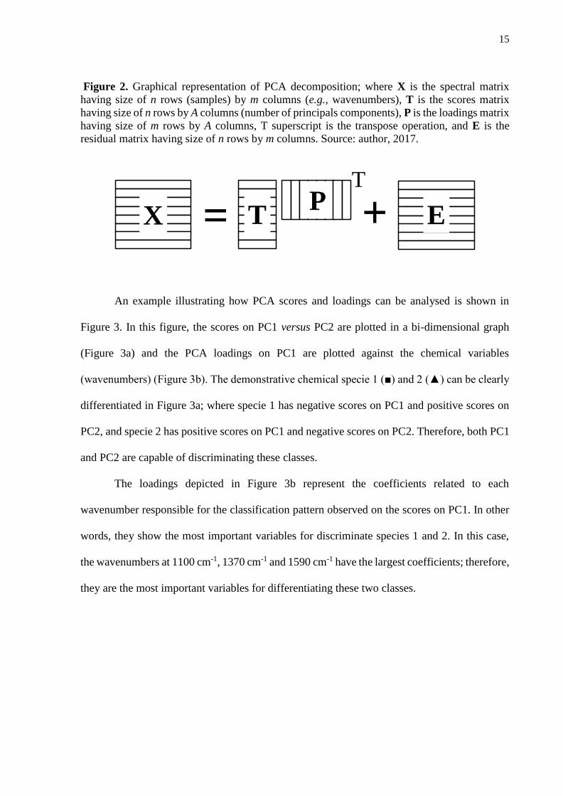
Principal Component Analysis with Linear and Quadratic Discriminant Analysis for Identification of Cancer Samples Based on Mass Spectrometry
Camilo L. M. Morais and Kássio M. G. Lima*
Química Biológica e Quimiometria, Instituto de Química, Universidade Federal do Rio Grande do Norte, 59072-970 Natal-RN, Brazil
Mass spectrometry (MS) is a powerful technique that can provide the biochemical signature of a wide range of biological materials such as cells and biofluids. However, MS data usually has a large range of variables which may lead to difficulties in discriminatory analysis and may require high computational cost. In this paper, principal component analysis with linear discriminant analysis (PCA-LDA) and quadratic discriminant analysis (PCA-QDA) were applied for discrimination between healthy control and cancer samples (ovarian and prostate cancer) based on MS data sets. In addition, an identification of prostate cancer subtypes was performed. The results obtained herein were very satisfactory, especially for PCA-QDA. Selectivity and specificity were found in a range of 90-100%, being equal or superior to support vector machines (SVM)-based algorithms. These techniques provided reliable identification of cancer samples which may lead to fast and less-invasive clinical procedures.
Keywords: mass spectrometry, classification, ovarian cancer, prostate cancer, QDA
Introduction
Mass spectrometry (MS) is an analytical technique that is used for determining the chemical composition of a given sample, to quantify compounds,1 and to help elucidate molecular structures.2,3 This technique has been increasingly utilized in biomedical and clinical research,4 since it can overcome many limitations of classical immunoassays5,6 and supports the development of fast and less-invasive clinical procedures.7-9
MS is usually coupled with chromatography such as liquid chromatography (LC-MS) and gas chromatography (GC-MS). Other techniques such as surface-enhanced laser desorption ionization time-of-flight (SELDI-TOF) and matrix-assisted laser desorption ionization time-of-flight (MALDI-TOF) are often used in MS applications, including disease screening and diagnosis.5 Some examples of MS applications includes toxicology screening and toxic drug quantification using quadrupole MS/MS;10 identification of inborn errors in metabolism or genetic defects in newborns for prenatal screening programs using electrospray tandem MS;11 detection of drug-induced hepatotoxicity using MS-based metabolomics;12 and identification and quantification of bleomycin in serum and tumor tissue by
high resolution LC-MS.13 MS-based techniques have been largely employed for cancer identification, such as for breast cancer,14 prostate cancer,15,16 ovarian cancer,17 lung cancer,18 and pancreatic cancer;19 as well as for identifying many biomarkers.18,20-24
One of the main fields using MS data is metabolomics, which aims to identify and quantify small molecules involved in metabolic reactions.25 Metabolomics studies have been applied in several areas, especially cancer.26 These analyses are typically performed in either targeted or untargeted approaches.25 The target approach aims to identify and quantify specific metabolites or metabolite class; whereas in the untargeted analysis a new hypothesis for further tests is generated by measuring all the metabolites in a biological system.25 To make this possible, multivariate statistical analysis is commonly employed in metabolomics studies by means of unsupervised or supervised classification techniques.25
Various types of chemometric algorithms have been reported for pattern recognition and classification of MS data, especially for discriminating between healthy control and cancer samples, or discriminating cancer subtypes. For instance, there are several papers reporting the use of partial least squares discriminant analysis (PLS-DA),14,18,20 hierarchical cluster analysis (HCA),14,27,28 principal component analysis (PCA),14,29 support vector machines
32
Principal Component Analysis with Linear and Quadratic Discriminant Analysis for Identification of Cancer Samples J. Braz. Chem. Soc.2
(SVM),17,29 artificial neural networks (ANN),28 principal-component analysis followed by linear discriminant analysis (PCA-LDA),15 principal component directed partial least squares (PC-PLS),30 and backward variable elimination partial least squares discriminant analysis (BVE-PLSDA).31
Principal component analysis (PCA) is a method of exploratory analysis capable of reducing the original data into a few variables.32 PCA reduces the data into a few principal components (PCs), where each one represents a piece of the original information. The first PC has the largest explained variance; therefore, they represent most of the information present in the original data. Using PCA, for instance, it is possible to reduce a large MS data set of thousands of variables into a few PCs representing the majority of the original information in just a few seconds. The PCA scores can be used as discriminant variables in conjunction with supervised classification techniques, such as linear discriminant analysis (LDA) and quadratic discriminant analysis (QDA). LDA is one of the most common algorithms used in supervised classification of 1st order spectral data, especially for spectroscopy applications in discriminatory analysis of cancer samples.33 On the other hand, there are only a few applications of QDA algorithm for discriminatory analysis reported in literature, and even fewer for QDA coupled to other chemometric techniques.33 QDA is a very simple algorithm, and differently from LDA, it computes the variance structures for each class separately,34 creating a more powerful discrimination rule for classes with different covariance matrices, such as for biological spectra sets in which the variability within classes is a key issue.
LDA has been reported in many MS applications, including analysis of N-glycans of human serum α1-acid glycoprotein (AGP) in cancer and healthy individuals;35 differentiation of vegetable oils;36 ovarian cancer detection based on proteomics;37 estimating false discovery rate (FDR) in phosphopeptide identifications;38 discrimination of ionic liquid types (ILs);39 and gasoline classification.40 QDA applications are fewer, and include characterization of ILs;39 identification of ovarian cancer;41 and gasoline classification.40
In this paper, principal component analysis followed by linear discriminant analysis (PCA-LDA) and quadratic discriminant analysis (PCA-QDA) were compared for discrimination between healthy controls and cancer (ovarian and prostate) samples. In addition, a further classification between benign subtypes of prostate cancer (serum PSA (prostate-specific antigen) 4-10 ng mL-1 and serum PSA > 10 ng mL-1) was performed. These algorithms take advantage of the power of MS-based techniques for
clinical analysis and provide a simple, fast, and reliable way to identify cancer samples.
Experimental
Samples
Data set 1: ovarian cancerThis data set is public available by Guan et al.17 It is
composed of LC/TOF-MS mass spectra (positive mode) from 35 healthy control (H.C.) and 37 ovarian cancer (O.C.) samples based on serum metabolomics. Retention time was not considered as a factor for chemometric modeling, thus the entire mass spectra (m/z values varying from 134.9919 to 1.4879 × 10³, having 360 variables) was integrated into an interval of retention time of 0-180 min. The control population consisted of patients with histology considered within normal limits and women with non-cancerous ovarian conditions; and the ovarian cancer samples were composed of patients with papillary serous ovarian cancer (stage I-IV). More details about the sample acquisition can be found in Guan et al.17
Data set 2: prostate cancerThis data set is public available by Petricoin III et al.16
It is composed of SELDI-TOF mass spectra from 63 healthy control (H.C.) and 69 prostate cancer (P.C.) samples based on serum proteomics. The m/z values varied from 0 to 1.9996 × 10⁴, having 15,153 variables. The control population was composed of men with no previous history of prostate cancer and serum PSA < 1 ng mL-1. The prostate cancer samples were acquired from patients with serum PSA ≥ 4 ng mL-1, digital rectal exam (DRE) evidence and single sextant biopsy evidence of prostate cancer (Gleason scores 4-9). More details about the sample acquisition can be found in Petricoin III et al.16
Data set 3: subtypes of prostate cancerThis data set was also obtained from Petricoin III et al.16
It is composed of SELDI-TOF mass spectra from 26 prostate cancer samples with PSA 4-10 ng mL-1 (low grade) and 43 prostate cancer samples with PSA > 10 ng mL-1 (high grade). These data are derived from data set 2 (m/z values varying from 0 to 1.9996 × 10⁴, having 15,153 variables) and more details about the sample acquisition can be found in Petricoin III et al.16
Computational analysis
The data treatment and chemometric analysis were performed using MATLAB® software R2012b42
33
Morais and Lima 3Vol. 00, No. 00, 2017
(MathWorks, USA) with PLS Toolbox 7.9.3 (Eigenvector Research, Inc., USA). All data sets were normalized by Euclidian norm and baseline corrected using automatic Whittaker filter (λ = 100, p = 0.001).43 Data sets 2 and 3 were mass drift corrected by using the icoshift algorithm44,45 in the m/z range of 3000-10000. Mean-centering scaling was applied to the data before chemometric modelling.
The samples for each data set were divided into training (ca. 70%), validation (ca. 15%) and prediction (ca. 15%) sets by using the Kennard-Stone uniform sample selection algorithm.46 Table 1 summarizes the number of samples for training, validation and prediction in each data set.
The chemometric models of PCA-LDA and PCA-QDA were built by firstly performing a principal component analysis (PCA),32 and then the A firstly scores selected were utilized as classification variables in a linear discriminant analysis (LDA) and quadratic discriminant analysis (QDA) model. The LDA classification score (Lik) and the QDA classification score (Qik) are calculated for a given class k by the following equations:47,48
(1)
(2)
where xi is the vector containing the classification variables for sample i; is the mean vector of class k; Σpooled is the pooled covariance matrix; and πk is the prior probability of class k. The pooled covariance matrix Σpooled and the prior probability πk are calculated as follows:47,48
(3)
(4)
where n is the total number of objects in the training set; K is the number of classes; nk is the number of objects of class k; and Σk is the variance-covariance matrix of class k, estimated by:48
(5)
The LDA and QDA classification scores (equations 1 and 2, respectively) were calculated based on the Mahalanobis distance modified by the fraction of samples in each class. In that case, they do not depend of scale, thus being dimensionless. These scores were used to calculate the discriminant function (DF) between the two classes as follows:48
DFLDA = Li1 – Li2 (6)DFQDA = Qi1 – Qi2 (7)
where Qi1 and Qi2 are the quadratic classification scores for classes 1 and 2, respectively.
If the DF result is positive for a given sample, the sample is closer to class 2, therefore it is classified as class 2; and if the DF result is negative for a given sample, the sample is closer to class 1, therefore being classified as class 1. In this sense, on the DF plot the class 2 is constituted of all positive values; whereas class 1 is constituted of all negative values. A flowchart illustrating the MS data processing is shown in Figure 1.
Although both LDA and QDA are based on a Mahalanobis distance calculation, the QDA algorithm forms a separated variance model for each class, not assuming that classes have similar variance-covariance matrices as LDA does.34 Therefore, QDA is more suitable to build classification models of data having different variance structures, such as what happens in many biological data sets.
Table 1. Number of samples in the training, validation and prediction sets for each data set
Training Validation Prediction
Data set 1 50 10 12
Data set 2 92 19 21
Data set 3 48 10 11
Figure 1. Flowchart illustrating MS data processing.
34
Principal Component Analysis with Linear and Quadratic Discriminant Analysis for Identification of Cancer Samples J. Braz. Chem. Soc.4
Quality performance
The performances of the employed algorithms were evaluated according to the following quality metrics: accuracy, sensitivity, specificity, positive and negative predictive value, Youden’s index, and positive and negative likelihood ratios. Accuracy is related to the percentage of correct classification;49 sensitivity (SENS) is the confidence that a positive result for a sample of the labeled class is obtained; specificity (SPEC) is the confidence that a negative result for a sample of the non-labeled class is obtained; positive predictive value (PPV) measures the proportion of positives that are correctly assigned; negative predictive value (NPV) measures the proportion of negatives that are correctly assigned; Youden’s index (YOU) evaluates the classifier’s ability to avoid failure; positive likelihood ratio (LR+) is the ratio between the probability of predicting an example as positive when it is truly positive and the probability of predicting an example as positive when it is not positive; and negative likelihood ratio (LR–) is the ratio between the probability of predicting an example as negative when it is actually positive and the probability of predicting an example as negative when it is truly negative.33 The equations of these quality parameters are shown in Table 2.
Results and Discussion
Data set 1: ovarian cancer
Ovarian cancer encompasses a heterogeneous group of tumors having differences in epidemiological and genetic risk factors, precursor lesions, spread patterns, molecular events during oncogenesis, response to chemotherapy and prognosis. Most ovarian cancers (90%) are malignant epithelial tumors named carcinomas, and the remaining
are germ cells and sex cord-stromal tumors.50 This type of cancer is the leading cause of death from gynecological malignances, and its mortality is a consequence of late presentation and diagnosis at stages III or IV, resulting in five-year survival rates of 20 and 6%, respectively.33 A study using serum metabolomics by MS-based techniques could lead to a faster and more robust classification of cancer and non-cancer patients. In this data set, the baseline corrected LC/TOF-MS mass spectra of healthy control (H.C.) and ovarian cancer (O.C.) samples are shown in Figure 2a. As can be seen, the signals are very superposed and no visual differentiation between H.C. and O.C. can be made.
Figure 2. (a) Baseline corrected mass spectra for healthy control (H.C.) and ovarian cancer (O.C.) samples; (b) PCA scores on PC1 versus scores on PC2 for healthy control (H.C.) and ovarian cancer (O.C.) samples, where the percentage of total variance described by each PC is described inside parenthesis. The circled blue line is the confidence ellipse of 95%.
Table 2. Quality parameters
Parameter Equation
Accuracy / %
Sensitivity / %
Specificity / %
Positive predictive value / %
Negative predictive value / %
Youden’s index / %
Positive likelihood ratio
Negative likelihood ratio
y = total number of samples incorrectly classified for a set of N samples; TP: true positive; TN: true negative; FP: false positive; FN: false negative; SENS: sensitivty; SPEC: specificity.
35
Morais and Lima 5Vol. 00, No. 00, 2017
Using PCA for exploratory analysis of this data set, the scores plot on the 1st and 2nd PCs is depicted in Figure 2b. Although PCA technique could be used as a classification tool, the lack of discrimination pattern in this scores plot leads to the use of supervised discriminant analysis. PCA-LDA and PCA-QDA were applied to the 10 first PCs (cumulative explained variance of 86.33%) and its DF plots are shown in Figures 3a and 3b, respectively. These figures show a better discriminant pattern for differentiating H.C. and O.C. samples.
The PCA-QDA DF plot also suggests a difference in variance structures between the classes, where the ovarian cancer sample set has a higher covariance matrix since this class has higher DF values than the other. This is probably caused by the high complexity of ovarian cancer disease as mentioned earlier. The quality performance parameters found for these chemometric models are shown in Table 3.
As shown in Table 3, the best quality parameters were obtained for PCA-QDA (accuracy in prediction set = 91.67%). On the other hand, PCA-LDA only achieved accuracy of 58.33% in prediction and 30% in the validation set. The low accuracy in the validation set suggests that the model is not well fitted, reflecting its poor prediction ability. PCA-QDA probably had superior performance because the classes’ variance structures are very different due to the high composition variability of the ovarian cancer samples, which increases the power of QDA compared to LDA. The accuracy in prediction set of PCA-QDA is close to what was obtained in literature using SVM, a more robust algorithm.17 Sensitivity and specificity were also equal to 91.67%, being superior to the results achieved by linear and non-linear SVM classifiers applied to this data set (sensitivity = 78.4 and 83.8%, respectively; and specificity = 74.3 and 77.1%, respectively).17 In addition, the classification results using PCA-QDA were superior than those ones found by applying PCA-SVM using a radial bases function (RBF) kernel to
this data set. PCA-SVM shown accuracy, sensitivity and specificity all equal to 75%, therefore being an algorithm with intermediary performance between PCA-LDA and PCA-QDA to classify H.C. and O.C. samples. Moreover, the high value of LR+ and the low value of LR– prove that PCA-QDA is superior for identifying cancer, since these parameters are directly related to the clinical concept of “ruling-OUT” and “ruling-IN” disease, respectively.33
From 360 variables present in this MS data set, only 31 were found to be statistical significant between the two classes (p < 0.05) (see Figure S7 in Supplementary Information (SI)). Among these variables, seven presented mean intensity variations (∆I) higher than 1%. These
Figure 3. DF plot for (a) PCA-LDA and (b) PCA-QDA models for discriminating healthy control (H.C.) and ovarian cancer (O.C.) samples. The DF scale for the QDA-based models were zoomed to improve visualization.
Table 3. Quality performance parameters found for PCA-LDA and PCA-QDA models for discriminating healthy control and ovarian cancer samples.
ParameterModel
PCA-LDA PCA-QDA
Accuracy
Training set / % 70.00 84.00
Validation set / % 30.00 70.00
Prediction set / % 58.33 91.67
Sensitivity / % 58.33 91.67
Specificity / % 58.33 91.67
PPV / % 58.33 91.67
NPV / % 58.33 91.67
YOU / % 16.67 83.33
LR+ 1.40 11.00
LR– 0.71 0.09
PCA-LDA: principal component analysis with linear discriminant analysis; PCA-QDA: principal component analysis with quadratic discriminant analysis; PPV: positive predictive value; NPV: negative predictive value; YOU: Youden’s index; LR+: positive likelihood ratio; LR–: negative likelihood ratio.
36
Principal Component Analysis with Linear and Quadratic Discriminant Analysis for Identification of Cancer Samples J. Braz. Chem. Soc.6
m/z values were 279.1263 (∆I = –14.71%), 496.3121 (∆I = 6.97%), 496.3139 (∆I = 8.99%), 520.3164 (∆I = 4.98%), 520.3169 (∆I = 4.59%), 524.3463 (∆I = 4.33%) and 991.6178 (3.75%). The negative signal implies that the peak is more intense in O.C. class, while the positive signal implies that the peak is more intense in H.C. class. The m/z values of 496.3121, 496.3139, 520.3164, 520.3169 and 524.3463 are associated with types of lysophosphatidylcholine (LysoPC),51 a metabolite identified in plasma that is directly related to the presence of ovarian cancer.52 The other m/z values have not been reported or associated with any cancer metabolite according to The Human Metabolome Database (HMDB).51
Data set 2: prostate cancer
Prostate cancer is the most commonly diagnosed male malignant cancer in the world. It has an incidence rate of 214 cases per 100,000, and a mortality rate from metastatic disease of 30 in 100,000.53 Prostate tissue is structurally
complex, being primarily constituted of glandular ducts lined by epithelial cells and supported by heterogeneous stroma. Its identification is very invasive and analyst-dependent, being subject to intra- and inter-observer errors.54 A study using serum proteomics by MS-based techniques could lead to a faster and more robust classification of cancer and non-cancer patients. In this data set, SELDI-TOF mass spectra of healthy control (H.C.) and prostate cancer (P.C.) samples were utilized. Figure 4a shows the baseline corrected mass spectra for these two classes. The signal complexity present in Figure 4a shows how difficult it is to differentiate one class from another, therefore requiring pattern recognition algorithms. Initially, PCA was utilized as exploratory analysis, and its scores plot is shown in Figure 4b.
No clear discriminant pattern is observed in the PCA scores graph. On the other hand, the results improved significantly by applying LDA and QDA to the PCA scores. PCA-LDA and PCA-QDA DF plots are shown in Figures 5a and 5b, respectively. 10 PCs were utilized (cumulative explained variance of 81.11%) for classification.
Figure 4. (a) Baseline corrected mass spectra for healthy control (H.C.) and prostate cancer (P.C.) samples; (b) PCA scores on PC1 versus scores on PC2 for healthy control (H.C.) and prostate cancer (P.C.) samples, where the percentage of total variance described by each PC is described inside parenthesis. The circled blue line is the confidence ellipse of 95%.
Figure 5. DF plot for (a) PCA-LDA and (b) PCA-QDA models for discriminating healthy control (H.C.) and prostate cancer (P.C.) samples. The DF scale for the QDA-based models were zoomed to improve visualization.
37
Morais and Lima 7Vol. 00, No. 00, 2017
Figure 5 shows a clear separation between the two classes using both PCA-LDA and PCA-QDA, where PCA-QDA had a slightly better classification. As seen in the DF plot of PCA-QDA, the healthy control samples have a higher variance structure than prostate cancer samples. This variability within this biological class may be related to different habits and lifestyles of the patients.53 The quality performance parameters found for PCA-LDA and PCA-QDA models are shown in Table 4.
Table 4 shows the notable performance of the tested algorithms. PCA-LDA and PCA-QDA had accuracy in the prediction set of 100%, being 5% above the value found in literature for prostate cancer detection based on this data set.16 The LR+ values equal to infinite are a consequence of LR+ equation shown in Table 2, because when the specificity is close to 100%, this parameter tends to infinite. The sensitivity and specificity of PCA-LDA and PCA-QDA were equal to 100%, being above the values found using a bioinformatics algorithm based on cluster analysis of topological feature maps (sensitivity = 95%, specificity = 71%).16 Using PCA-SVM with RBF kernel, an accuracy, sensitivity and specificity of 100% were also found. However, the complexity degree employed during SVM is much higher than LDA and QDA, meaning that with simpler algorithms the same classification performance can be obtained.
From a total of 15,153 variables in the original data, 5,583 were found to be statistical significant between the two classes (p < 0.05) (see Figure S8 in SI). The larger number of variables as well as the untargeted procedure and the
complexity of this proteomic data make nearly impossible to identify important molecules based on these 5,583 variables.
The use of PCA-LDA and PCA-QDA in this data set of serum proteomics provides a reliable, non-analyst dependent and less-invasive differentiation between patients with no evidence of prostate cancer and patients with prostate cancer. This can be a powerful tool for clinical screening, avoiding patients to suffer unnecessary surgical procedures, for instance.
Data set 3: subtypes of prostate cancer
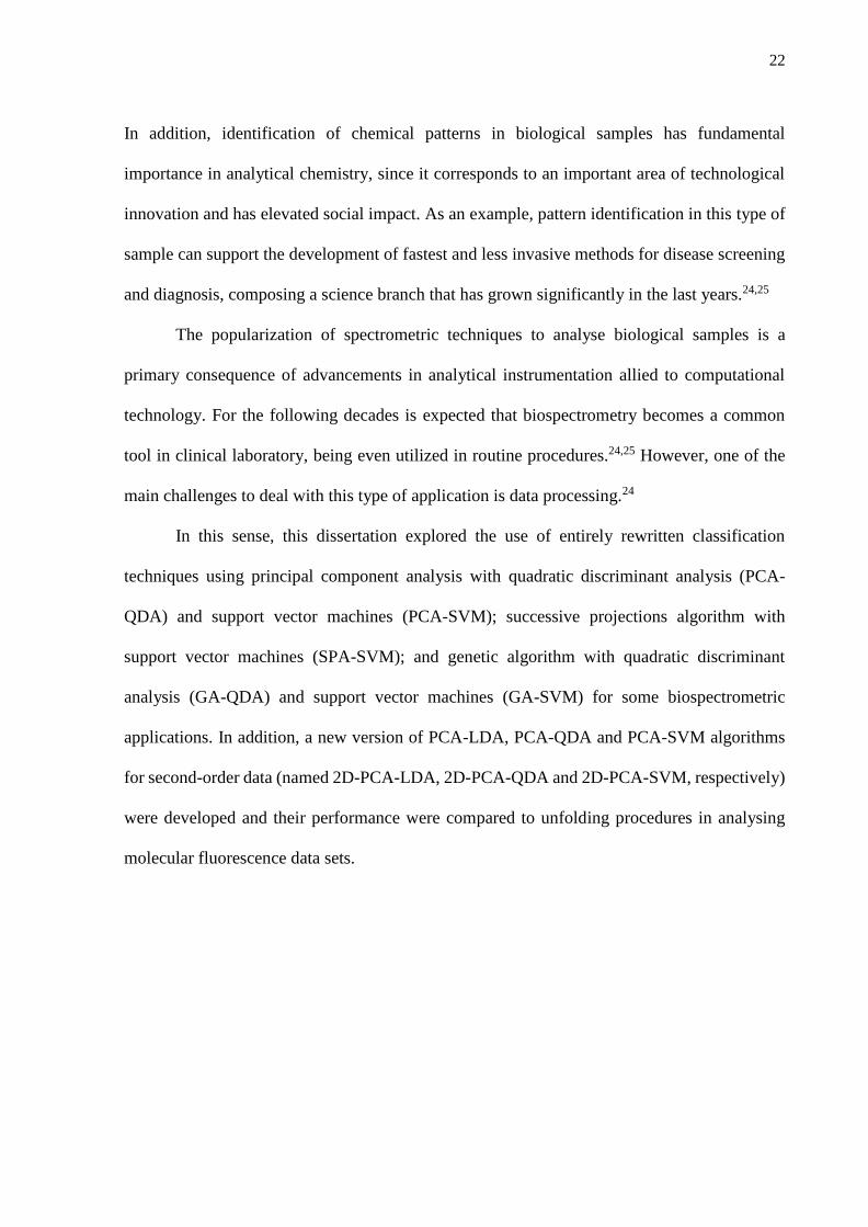
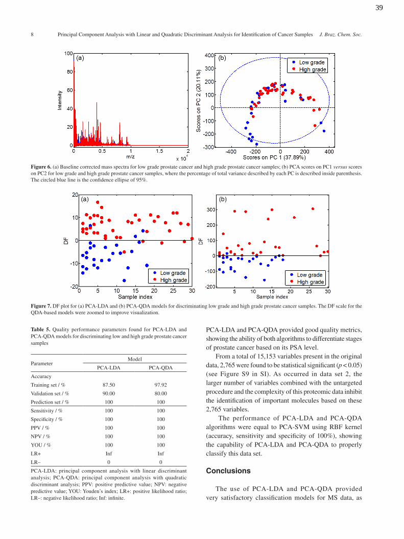
This data set is derived from data set 2, where the cancer samples were divided into two classes: class 1 having cancer samples with serum PSA 4-10 ng mL1 (low grade); and class 2 having cancer samples with serum PSA > 10 ng mL-1 (high grade). This data set was created to evaluate the power of the algorithms to differentiate cancer samples according to its stage. Although PSA is not a final indicator of prostate cancer, it is important to differentiate low and high PSA levels, since the PSA indicates during clinical screening if a patient will need a more robust/invasive exam or not. Usually, patients with low PSA levels but with suspicion of prostate cancer undergo an additional DRE exam. However, it is recommended that patients with high PSA levels undergo additional DRE tests, such as transrectal ultrasound and cystoscopy.55,56 The baseline corrected mass spectra of the low grade and high grade cancer samples are shown in Figure 6a.
Figure 6b shows the PCA scores for low and high grade samples, where no discriminant profile is seen. By applying PCA-LDA and PCA-QDA to the data (10 PCs, cumulative explained variance of 86.29%), the differentiation between the two classes improves significantly, as shown in Figures 7a and 7b, respectively. An almost perfect separation between the two classes is obtained in the PCA-QDA DF plot.
The coefficients in the PCA-QDA DF plots show that the variances of the low and high grade classes are similar to each other, with a bit higher covariance matrix for the high grade samples. Table 5 shows the quality parameters found by the chemometric models applied to this data set.
For classification purposes, the PCA-LDA and PCA-QDA models had very similar performances, with sensitivity and specificity of 100% each. The training ability of PCA-QDA was better than PCA-LDA, but the algorithm had worst performance in the validation set. The poorer classification in the training and validation set for both algorithms when compared to the prediction set is a possible result of the reduced number of samples. Nevertheless, the maximum results obtained in the prediction set with
Table 4. Quality performance parameters found for PCA-LDA and PCA-QDA models for discriminating healthy control and prostate cancer samples
ParameterModel
PCA-LDA PCA-QDA
Accuracy
Training set / % 95.65 96.74
Validation set / % 100 100
Prediction set / % 100 100
Sensitivity / % 100 100
Specificity / % 100 100
PPV / % 100 100
NPV / % 100 100
YOU / % 100 100
LR+ Inf Inf
LR– 0 0
PCA-LDA: principal component analysis with linear discriminant analysis; PCA-QDA: principal component analysis with quadratic discriminant analysis; PPV: positive predictive value; NPV: negative predictive value; YOU: Youden’s index; LR+: positive likelihood ratio; LR–: negative likelihood ratio; Inf: infinite.
38
Principal Component Analysis with Linear and Quadratic Discriminant Analysis for Identification of Cancer Samples J. Braz. Chem. Soc.8
PCA-LDA and PCA-QDA provided good quality metrics, showing the ability of both algorithms to differentiate stages of prostate cancer based on its PSA level.
From a total of 15,153 variables present in the original data, 2,765 were found to be statistical significant (p < 0.05) (see Figure S9 in SI). As occurred in data set 2, the larger number of variables combined with the untargeted procedure and the complexity of this proteomic data inhibit the identification of important molecules based on these 2,765 variables.
The performance of PCA-LDA and PCA-QDA algorithms were equal to PCA-SVM using RBF kernel (accuracy, sensitivity and specificity of 100%), showing the capability of PCA-LDA and PCA-QDA to properly classify this data set.
Conclusions
The use of PCA-LDA and PCA-QDA provided very satisfactory classification models for MS data, as
Figure 6. (a) Baseline corrected mass spectra for low grade prostate cancer and high grade prostate cancer samples; (b) PCA scores on PC1 versus scores on PC2 for low grade and high grade prostate cancer samples, where the percentage of total variance described by each PC is described inside parenthesis. The circled blue line is the confidence ellipse of 95%.
Figure 7. DF plot for (a) PCA-LDA and (b) PCA-QDA models for discriminating low grade and high grade prostate cancer samples. The DF scale for the QDA-based models were zoomed to improve visualization.
Table 5. Quality performance parameters found for PCA-LDA and PCA-QDA models for discriminating low and high grade prostate cancer samples
ParameterModel
PCA-LDA PCA-QDA
Accuracy
Training set / % 87.50 97.92
Validation set / % 90.00 80.00
Prediction set / % 100 100
Sensitivity / % 100 100
Specificity / % 100 100
PPV / % 100 100
NPV / % 100 100
YOU / % 100 100
LR+ Inf Inf
LR– 0 0
PCA-LDA: principal component analysis with linear discriminant analysis; PCA-QDA: principal component analysis with quadratic discriminant analysis; PPV: positive predictive value; NPV: negative predictive value; YOU: Youden’s index; LR+: positive likelihood ratio; LR–: negative likelihood ratio; Inf: infinite.
39
Morais and Lima 9Vol. 00, No. 00, 2017
demonstrated for MS-based serum metabolomics in the detection of ovarian cancer; and also MS-based serum proteomics for the detection of prostate cancer and its subtypes according to the PSA level. The LDA and QDA-based algorithms are very simple compared to many other algorithms utilized in literature, such as SVM, and can also provide very solid classification results; especially PCA-QDA, which models the data considering different variance structures between the classes. Apart from the very satisfactory classification results found for the tested data sets (sensitivity and specificity > 90%), these algorithms also significantly reduce the data, which considerably speeds up the computational analysis, enabling a supervised classification of an MS data set of thousands of variables in less than one minute, for example. The speed and solid classification results found by these algorithms for the tested applications show that they combine very well with the power of MS-based techniques, thus being capable to be utilized in other types of applications in the future. The combination of MS-based serum analysis and these types of chemometric techniques can provide very acceptable findings for developing fast, very accurate, less-invasive, and non-analysis dependent clinical procedures, especially for screening purposes.
Supplementary Information
Supplementary information is available free of charge at http://jbcs.sbq.org.br as PDF file.
Acknowledgments
Camilo L. M. Morais would like to acknowledge the financial support from CAPES/PPGQ/UFRN for his research grant. K. M. G. Lima acknowledges the CNPq grant (305962/2014-0) for financial support.
References
1. Vogester, M.; Seger, C.; Clin. Biochem. 2016, 49, 947.
56. Oesterling, J. E.; Rice, D. C.; Glenski, W. J.; Bergstralh, E. J.;
Urology 1993, 42, 276.
Submitted: March 23, 2017
Published online: September 5, 2017
41
42
CHAPTER 3 – VARIABLE SELECTION WITH A SUPPORT VECTOR MACHINE FOR
DISCRIMINATING Cryptococcus FUNGAL SPECIES BASED ON ATR-FTIR
SPECTROSCOPY
Camilo L. M. Morais
Fernanda S. L. Costa
Kássio M. G. Lima
Manuscript published in Analytical Methods, 2017, 9, 2964–2970.
Author contributions: C.L.M.M. developed the algorithms; applied the algorithms to
process the data; interpreted results; and wrote the manuscript. F.S.L.C. produced
experimental data. K.M.G.L. supervised the project.
______________________________
Camilo L. M. Morais
______________________________
Kássio M. G. Lima
Variable selection with a support vector machinefor discriminating Cryptococcus fungal speciesbased on ATR-FTIR spectroscopy
Camilo L. M. Morais, Fernanda S. L. Costa and Kassio M. G. Lima *
Variable selection with supervised classification is currently an important tool for discriminating biological
samples. In this paper, 15 supervised classification algorithms based on a support vector machine (SVM)
were applied to discriminate Cryptococcus neoformans and Cryptococcus gattii fungal species using
ATR-FTIR spectroscopy. These two fungal species of the Cryptococcus genus are the etiological agents
of Cryptococcosis, which is an opportunistic or primary fungal infection with global distribution. This
disease is potentially fatal, especially for immunocompromised patients, like those suffering from AIDS.
The multivariate classification algorithms tested were based on principal component analysis (PCA),
successive projections algorithm (SPA) and genetic algorithm (GA) as data reduction and variable
selection methods, being coupled to a SVM with different kernel functions (linear, quadratic, 3rd order
polynomial, radial basis function, and multilayer perceptron). Some of these algorithms achieved very
successful classification rates for discriminating fungal species, with accuracy, sensitivity, and specificity
equal to 100% using both SPA-SVM-polynomial and GA-SVM-polynomial algorithms. These results show
the potential of such techniques coupled to ATR-FTIR spectroscopy as a rapid and non-destructive tool
for classifying these fungal species.
Introduction
Cryptococcosis is an opportunistic fungal infection caused byinhaling basidiospores1 or dissected yeasts present in theenvironment, causing an infection of the central nervoussystem which affects immunocompromised individuals,including AIDS patients and organ transplant recipients orother patients receiving immunosuppressive drugs.2,3 Thisdisease affects the respiratory tract of the host causing severepneumonia and respiratory insufficiency and is responsible forthe majority of worldwide deaths from HIV-related fungalinfections.1,3
The main etiologic agents of Cryptococcosis in humans aretwo species, namely Cryptococcus neoformans (serotypes A, Dand AD) and Cryptococcus gattii (serotypes B and C), which differin their epidemiology, host range, virulence, antifungalsusceptibility and geographic distribution.1 Cryptococcus gattiiis a primary pathogen which infects immunocompetent andhealthy individuals, having predilection for the lungs.4 On theother hand, Cryptococcus neoformans has predilection for thecentral nervous system and mainly infects immunosuppressedpatients mostly having HIV/AIDS.5 Cryptococcus gattii isresponsible for many infection cases in the Pacic Northwest ofthe United States.6 This high virulence occurs due to an unusual
tubular mitochondrial morphology caused by mitochondrialfusions to enhance the repair of mitochondrial DNA damagefrom oxidative stress within the phagosome.4 In addition,Cryptococcus gattii has two metabolites of acetoin and dihy-droxyacetone which potentially produce less pro-inammatoryresponse than those of Cryptococcus neoformans. This facili-tates fungal survival and local multiplication causing morecryptococcomas.4 There are some morphological features thatare specically associated with each of the two species such astexture, pigmentation produced by their colonies, and yeastform.1,7 However, it is still more reliable to distinguish them bytheir growth phenotype on certain media formulations basedon their biochemical differences.8
Cryptococcosis is a treatable disease, however its effects aredevastating to the patients, resulting in death or central nervoussystem dysfunction unless the condition is diagnosed andtreated at the time of onset.1 Currently, the techniques used inthe identication of these pathogens are direct microscopicexamination and molecular methods such as DNA hybridiza-tion and PCR-based methods (particularly nested, multiplexand real time PCR).9,10 These methods provide both highsensitivity and specicity; however, most have some limitationsthat may hinder the nal diagnosis, further requiring severaldays to detect and identify the microorganisms.10
In order to improve the ability to properly control fungalinfections in humans, early identication of the pathogen isnecessary, since they have different responses to antifungal
Biological Chemistry and Chemometrics, Institute of Chemistry, Federal University of
Rio Grande do Norte, Natal 59072-970, RN, Brazil. E-mail: [email protected]
Cite this: Anal. Methods, 2017, 9, 2964
Received 17th February 2017Accepted 11th April 2017
treatments.11 In this sense, Fourier transform infrared spec-troscopy (FTIR) has been standing out in the past few years inthe microbiological area,12,13 because it provides a large amountof information about typical absorption bands for each func-tional group, providing a spectroscopic ngerprint of the totalbiochemical and structural composition unique for eachmolecule.14 The mid-IR region at 1800–900 cm�1 contains thefundamental vibrational modes of key chemical bonds ofintracellular mechanisms corresponding to the biochemicalngerprint of the material under study, therefore being calledthe biongerprint region.14 In addition, FT-IR has the advan-tages of being rapid and non-destructive, using small samplesizes, and requiring an easy sample preparation.14
In attenuated total reection – Fourier transform infrared(ATR-FTIR), the ATR module enhances the signal by passing theIR beam through the sample, taking advantage of several internalreections with the crystal.15,16 Such reections generate anevanescent wave that penetrates the material to a depth between0.5 and 2 mm.16 ATR-FTIR has been very effective in analyzingbiological samples, as demonstrated in analyzing diverse types ofcancer,17 insects,18,19 and bacteria;20,21 as well as to monitor planthealth in a controlled22 and natural23 environment.
Good computation tools are required to follow the advancesin spectroscopy techniques applied to biological samples. Thesetools enable building classication models for screening anddiagnosis methods, which is a common task in biospectroscopyapplications.14 A very powerful multivariate classication tech-nique is the support vector machine (SVM).24 SVMs are binaryclassiers that work by nding a classication hyperplanewhich separates two classes or objects providing the largestmargin of separation.25 A key advantage of SVMs over mostother classical classication methods is that an SVM is capableof classifying nonlinearly separable data.25 This makes itsperformance superior to linear-dependent classicationmethods, such as linear discriminant analysis (LDA).25 Thekernel function is responsible for transforming the data intoa different feature space (linear, quadratic, and polynomial,among others) changing the classication ability of SVMs.26
SVM algorithm applications in biological data include classi-fying low-grade cervical cytology;27 breast cancer diagnosis;28
ovarian cancer identication;29 analysis of dengue infection;30
and classifying Candida fungi.31
Data reduction and variable selection methods can becoupled with the SVM algorithm in order to speed up compu-tational analysis. A common method of data reduction is prin-cipal component analysis (PCA).32 PCA reduces the original datato a few principal components (PCs) having most of the originalexplained variance;32 and the scores on each PC can be used asclassication variables for the SVM. Among the variable selec-tion methods, successive projections algorithm (SPA)33 andgenetic algorithm (GA)34 have found many applications in bio-logical data.17,18 SPA reduces the original data to few variables byminimizing its collinearity,33 while GA reduces the datafollowing an evolutionary process where the ttest set of vari-ables is chosen.34 Both algorithms maintain the original datadimension, being consequently used as a tool to search forspecic molecular fragments, also called biomarkers.14
In this paper, we have applied different types of algorithmsbased on PCA-SVM, SPA-SVM, and GA-SVM with different kernelfunctions (linear, quadratic, 3rd order polynomial, radial basisfunction, and multilayer perceptron) as a rapid and non-destructive method to discriminate Cryptococcus gattii andCryptococcus neoformans fungal species based on ATR-FTIRspectroscopy. In addition, a tentative assignment of possiblebiomarkers involved in differentiating these fungal species isperformed.
MethodsSample preparation
In this study, 28 isolated samples from UFPI (UniversidadeFederal do Piauı); IMT/SP (Instituto de Medicina Tropical deSao Paulo), Veterinary Hospital-UNESP, campus Botucatu (SP),FioCruz mycological collection and recently isolated fungusfrom Giselda Trigueiro Hospital (Natal/RN/Brazil) were used.Genotyping of the isolated fungus in culture on Sabouraud Agarwith Chloramphenicol (50 mg L�1) was done at the Institute ofTropical Medicine of RN at UFRN, using PCR-RFLP of the URA5gene as previously described,4 under approval of the ethicscommittee, number 51050415.6.0000.5537.
These fungi were incubated for 48 hours at a temperature of30 �C until satisfactory growth is achieved. Yeast cells wereinactivated for biosafety handling in the spectroscopy equip-ment by placing some yeast colonies in 1.0 mL of para-formaldehyde solution at 4% plus phosphate buffer (1 mol L�1)v/v, and in 1.5 mL eppendorf tubes for cell attachment toinactivate yeast cells. The nal solution was added to 28 tubeswith 28 different Cryptococcus isolates. Aer 3 hours at roomtemperature, the tubes with cells were placed under refrigera-tion at�20 �C until the next step. For spectra reading, the tubeswere put at room temperature until defrosted, and thencentrifuged for 10 minutes at 5000g for cell precipitation. Thesupernatant was removed and the cells were washed with 1.0mL of sterile saline solution (0.95% w/v). The tubes weremaintained at 4 �C until spectroscopy reading.
ATR-FTIR spectroscopy
The ATR-FTIRmeasurements (n¼ 280, 10 replicates of each oneof the 28 C. neoformans (n ¼ 14) and C. gattii (n ¼ 14) samples)were recorded using a Bruker VERTEX 70 FTIR spectrometer(Bruker Optics Ltd., UK) with Helios ATR attachment containinga diamond crystal internal reective element and a 45 incidenceangle of IR beam. The ATR-FTIR spectra of fungal samples wereacquired in the range of 400–4000 cm�1 with a resolution of 4cm�1. Each spectrum was collected at 16 scans in the absor-bancemode. Approximately 50 mL of each sample was applied tothe ATR crystal immediately following collection of each back-ground. A small piece of aluminum foil was placed on thesample to ensure that no air bubbles were trapped on the crystalsurface and to improve the signal-to-noise ratio of the spectra.35
The ATR crystal was cleaned with 70% v/v alcohol and a newbackground was collected prior to the analysis of a new sample
and compared to the rst background to ensure no interferencein the sample signal.
Computational analysis
Computational analysis was performed within a Matlab R2012benvironment (MathWorks, USA) by using PLS Toolbox version7.9.3 (Eigenvector Research, Inc., USA) and homemade algo-rithms. Raw spectral data were pre-processed by cutting theregion of 1800–900 cm�1, followed by normalization to theamide I peak (�1650 cm�1)15 and baseline correction.
Samples for training (n ¼ 196), validation (n ¼ 42), andprediction (n ¼ 42) sets were selected using the Kennard–Stoneuniform sampling selection algorithm.36 The training set wasused to build the classication models, and the validation set toevaluate its internal performance. The prediction set was onlyused in the nal classication evaluation.
The pre-processed spectra were utilized in the classicationalgorithms as follows: rst, data reduction was performed bymeans of PCA, SPA, and GA; utilizing PCA, the scores on the rstPCs were utilized as classication variables for the SVM;whereas during SPA and GA, the selected variables having thelowest average risk of miss classication G were utilized asclassication variables for the SVM. The G cost function iscalculated in the validation set as18
G ¼ 1
NV
XNV
n¼1
gn; (1)
where NV is the number of validation samples; and gn is denedas,
gn ¼r2�xn;mIðnÞ
�
minIðmÞsIðnÞr2�xn;mIðmÞ
� (2)
In eqn (2), the numerator is the squared Mahalanobisdistance between the object xn (of class index In) and the samplemean mI(n) of its true class; whereas the denominator is thesquared Mahalanobis distance between the object xn and themean mI(m) of the closest wrong class. GA was performedthrough 80 generations, having 160 chromosomes each.Crossover and mutation probability were set to 60% and 10%,respectively. The algorithm was repeated three times and thebest result was chosen.
Thereaer, the PCA-SVM, SPA-SVM, and GA-SVM modelswere constructed. Different types of SVM kernels were utilized:linear (L), quadratic (Q), 3rd order polynomial (P), radial basisfunction (RBF), and multilayer perceptron (MPL). Such kernelstransform the data into a feature space and are responsible forthe SVM classication ability.26 These kernels are calculated asfollows:26,37
Linear,
K(xi,zj) ¼ xTi zj (3)
Quadratic,
K(xi,zj) ¼ (s + xTi zj)2, s $ 0 (4)
3rd order polynomial,
K(xi,zj) ¼ (s + xTi zj)3, s $ 0 (5)
Radial basis function (RBF),
K(xi,zj) ¼ exp(�gkxi � zjk2) (6)
Multilayer perceptron (MLP),
K(xi,zj) ¼ tan h(k1xTi zj + k2) (7)
where xi and zj are sample measurement vectors; s is a constant;g is the parameter that determines the RBF width; and k1 and k2
are constants. The SVM classier takes the form of:
f ðxÞ ¼ sign
XNSV
i¼1
aiyiK�xi; zj
�þ b
!(8)
where NSV is the number of support vectors; ai is the Lagrangemultiplier; yi is the class membership (�1); K(xi,zj) is the kernelfunction; and b is the bias parameter.26,37
By using these distinct types of kernel functions, 15 algo-rithms were utilized for classifying the fungal species: PCA-SVM-L, PCA-SVM-Q, PCA-SVM-P, PCA-SVM-RBF, PCA-SVM-MLP, SPA-SVM-L, SPA-SVM-Q, SPA-SVM-P, SPA-SVM-RBF, SPA-SVM-MLP, GA-SVM-L, GA-SVM-Q, GA-SVM-P, GA-SVM-RBF,and GA-SVM-MLP. In the RBF kernel, the g parameter was setto 1; and in the MLP kernel, the k1 and k2 were respectively set to1 and �1. The s parameter was set to 0 for quadratic and 3rd
order polynomial kernels.
Statistical validation
The models were statistically evaluated according to accuracy,sensitivity, specicity, F-score, and G-score. Accuracy is relatedto the percentage of correct classication achieved by themodel; sensitivity measures the proportion of positive resultsthat are correctly identied; specicity measures the proportionof negative results that are correctly identied; F-score repre-sents the weighted average of the precision and sensitivity; andG-score accounts for the model precision and sensitivitywithout the inuence of positive and negative class sizes.38,39
where N is the total number of samples;H is the total number ofclasses; y*h is the number of samples incorrectly classied in theh class; TP is the number of true positives; TN is the number oftrue negatives; FP is the number of false positives; and FN is thenumber of false negatives.
Results and discussion
Cryptococcus gattii (C. gattii) and Cryptococcus neoformans(C. neoformans) fungals samples were acquired by ATR-FTIRspectroscopy in the region of 3200–800 cm�1. The raw spectrawere preprocessed by cutting the spectra at 1800–900 cm�1
corresponding to the biological ngerprint region; followed bynormalization to the amide I peak (�1650 cm�1) and baselinecorrection. The preprocessed spectra are shown in Fig. 1.
The difference in the between-mean spectrum of C. gattii andC. neoformans is shown in Fig. 2a. In this gure, it is possible toobserve that the large difference between the class' spectra is inthe amide I region (�1650 cm�1), where there is an absorbancedifference close to �4.5 � 10�3 (�4.6%). The negative signalimplies that this band is more intense in the C. neoformans class.A less intense difference between the class-mean is observed at�1035 cm�1, corresponding to glycogen bands.40 In addition, thespectral difference close to 900 cm�1 increases due to phospho-diester and protein phosphorylation absorptions.40,41
In order to classify these fungal species, the SVM was used asa classication technique based on PCA as data reduction; andSPA and GA as variable selection methods. The PCA modelapplied to these data reduced the 468 variables (as wave-numbers inside the 1800–900 cm�1 range) to only 3 PCs,accounting for 99.98% of explained cumulative variance. Fig. 2bshows the PCA loadings on PC1, PC2 and PC3. In this gure, theloadings on PC1 which account for the largest variance from theoriginal data (99.32% of explained variance) have higher coef-cients in the amide I peak region (�1650 cm�1), coincidingwith the largest between-mean spectrum difference depicted inFig. 2a. The loadings on PC2 (0.51% of explained variance) havehigher coefficients in the phosphodiester and protein phos-phorylation region (�900 cm�1). The loadings on PC3 (0.15% ofexplained variance) show high coefficients in the glycogenregion (�1035 cm�1). These bands evidenced by PCA loadings
are most important for class differentiation in the PCA-SVM-based models, which were built using ve types of kernelfunctions: linear (PCA-SVM-L), quadratic (PCA-SVM-Q), 3rd
order polynomial (PCA-SVM-P), RBF (PCA-SVM-RBF), and MLP(PCA-SVM-MLP).
In addition to PCA, SPA and GA were applied to reduce thenumber of variables and be further used with SVM classiers.The accuracy for each SVM-based algorithm in training, vali-dation, and prediction set is shown in Table 1.
The most accurate PCA-SVM algorithm in the prediction setwas composed of MLP kernel (PCA-SVM-MPL), which had85.7% accuracy, whereas the most accurate for SPA-SVM and
Fig. 1 Pre-processed spectra of C. gattii (blue color) and C. neofor-mans (red color) classes.
Fig. 2 (a) Difference between mean spectra of C. gattii and C. neo-formans classes. (b) PCA loadings on PC1 (blue color), PC2 (red color),and PC3 (green color).
Table 1 Accuracy (%) for SVM-based algorithms in training, validation,and prediction set
GA-SVM had 3rd polynomial kernel (SPA-SVM-P and GA-SVM-P)with an accuracy of 100%. The classication performance bymeans of sensitivity, specicity, F-score, and G-score for PCA-SVMs, SPA-SVMs, and GA-SVMs models is shown in Fig. 3.
As shown in Fig. 3, the PCA-SVM algorithm with the bestclassication performance was PCA-SVM-MPL, achievingsensitivity, specicity, F-score, and G-score equal to 85.7%. Forvariable selection, the best algorithms were SPA-SVM-P and GA-SVM-P, achieving sensitivity, specicity, F-score, and G-scoreequal to 100%. These classication rates of 100% show themodel's ability to correct the classication of all samples inwhich both positive and negative results were correctly identi-ed. The selected variables by SPA-SVM are shown in Table 2.The percentage of absorbance variation (DA) between theclasses at each selected wavenumber is also shown in this table.
Nine original wavenumbers were selected from 468 by SPA-SVM algorithms as classication variables. From the selectedwavenumbers, absorbance at 1635 cm�1 had the most intensevariation between the C. gattii and C. neoformans classes, witha variation of �4.4% (Table 2). This absorption is characteristicof the amide I b-sheet structure or proportions of b-sheetsecondary structures.40 The selected wavenumber at 906 cm�1
had the second largest DA (�2.4%). This wavenumber is in thephosphodiester region, composed of stretching of collagen andglycogen bands. The wavenumbers at 1443 cm�1 and 1745 cm�1
are respectively associated with the CH bending and symmetricstretching vibration of polysaccharides.40 The polysaccharidecapsules composed of 90–95% glucuronoxylomannan (GXM)and 5% galactoxylomannan (GalXM) determine the serotypes ofC. gattii (serotypes B and C) and C. neoformans (serotypes A, Dand AD) fungi,4 therefore being important for class differenti-ation. The less intense DA for the selected wavenumbers by theSPA-SVM algorithm was found at 1541 cm�1, a band of amide IIabsorption (N–H bending coupled to C–N stretching),40 which ischaracteristic of proteins predominantly in b-sheetconformation.42
The variables selected by the GA-SVM algorithm are shown inTable 3. In this case, GA-SVM selected 12 wavenumbers asclassication variables. Similar to Table 2, most of them havenegative DA values. These negative DA values show that mostselected wavenumbers have more intense absorption bands inthe C. neoformans class. The higher absorbance in this classcould be due to C. neoformans generally having a higherconcentration of metabolites than C. gattii,43 thereforeincreasing its absorption.
The higher DA for the selected wavenumbers by the GA-SVMalgorithm (Table 3) is at 912 cm�1 (�2.2%). This value is close tothe value obtained by the SPA-SVM algorithm at 906 cm�1 asshown in Table 2, and represents the phosphodiester region.The second largest DA was found at 991 cm�1 (DA ¼ �1.2%),being assigned as the vibration of C–O in ribose.40 This region isalso a characteristic of other carbohydrate molecules,15 there-fore its signal could have contributions from more than onebiomarker.
Amide I absorption was identied at 1697 cm�1 with DA of�1.0%. This band is a characteristic of high frequency vibrationof an antiparallel amide I b-sheet (in-plane C]O stretching
Fig. 3 Classification performance parameters (sensitivity, specificity,F-score, and G-score) for all SVM-based algorithms applied todiscriminate C. gattii and C. neoformans classes.
Table 2 Selected variables by SPA-SVM-based algorithms andtentative assignment of possible biomarkers
�) DNA/RNA �0.7�1443 d(CH) polysaccharides +0.4�1541 Amide II +0.03�1635 Amide I �4.4�1745 ns(C]O)
polysaccharides+0.2
a n ¼ stretching vibration; d ¼ bending vibration; ns ¼ symmetricstretching vibration. b Positive signal (+) indicates higher absorbancein the C. gattii class; negative signal (�) indicates higher absorbancein the C. neoformans class.
Table 3 Selected variables by GA-based algorithms and tentativeassignment of possible biomarkers
�) DNA +0.05�1278 Amide III +0.1�1323 Amide III +0.2�1508 Amide II +0.3�1697 Amide I �1.0�1734 ns(C]O) lipids +0.1
a ns ¼ symmetric stretching vibration; nas ¼ asymmetric stretching.b Positive signal (+) indicates higher absorbance in the C. gattii class;negative signal (�) indicates higher absorbance in the C. neoformansclass.
weakly coupled to C–N stretching and in-plane N–H bondbending).40 Other vibrations of almost the sameDAwas found at955 cm�1 (symmetric stretching of PO4
3�), 978 cm�1 (OCH3
vibration in polysaccharides), and 1070 cm�1 (symmetric PO2�
stretching in DNA/RNA).40 In this case, the inuence of thepolysaccharide capsules and nucleic acid contributions in thefungal species discrimination is clear. Amide II and amide IIIhad very small DA contributions (+0.1–0.3%). Amide II absorp-tion at 1508 cm�1 can be caused by N–H bending coupled toC–N stretching of amide II; whereas amide III absorptions at1278 cm�1 and 1323 cm�1 are associated with vibration modesof collagen proteins in amide III. The lower DA for GA-SVMalgorithms was found at 1248 cm�1 (DA ¼ +0.05) and corre-sponds to asymmetric PO2
� stretching in DNA.40
The results shown here corroborate to the development ofa rapid and non-destructive method for classifying C. gattii andC. neoformans fungal species with high accuracy, sensitivity, andspecicity by using ATR-FTIR spectroscopy coupled with SVM-based techniques. The non-destructive nature of ATR-FTIRspectroscopy enables to reuse the samples in further studies,including genotyping by PCR-based methods. In addition,variable selection techniques (SPA and GA) can help to identifypossible biomarkers responsible for class differentiation.
Furthermore, this research can be translated to real-worldcontinuous monitoring by using these techniques to analyzecerebrospinal uid of infected patients.1 ATR-FTIR spectroscopycombined with chemometric techniques could be used toreduce the volume of the uid utilized in the analysis, since theprocedure to extract this uid is quite invasive; as well as toreduce the cost, since the actual detection of both fungi followsgenotyping procedures using molecular methods. In addition,this study could be used as a support to try the detection of bothfungi in serum, which would reduce drastically the invasivenessof the procedure, allied to the advantages of using FTIR spec-troscopy reported before.
Conclusion
PCA, SPA and GA were coupled to SVM classiers to discrimi-nate C. gattii and C. neoformans fungal species. Five differenttypes of SVM kernels (linear, quadratic, 3rd order polynomial,RBF and MLP) were evaluated by means of quality metrics suchas accuracy, sensitivity and specicity providing high classi-cation rates. SPA-SVM and GA-SVM algorithms with 3rd orderpolynomial kernels (SPA-SVM-P and GA-SVM-P) achieved clas-sication rates of 100% in accuracy, sensitivity, specicity, F-score, and G-score, showing these models to have the ability toprovide reliable class differentiation. The SPA-SVM algorithmwas highly inuenced by amide I (1635 cm�1) and phospho-diester (906 cm�1) vibrations. In addition, the GA-SVM algo-rithm had higher inuences of C–O ribose (991 cm�1) andphosphodiester (912 cm�1) vibrations. This report supports thedevelopment of an alternative method to classify C. gattii and C.neoformans fungal species using ATR-FTIR spectroscopy, whichcould be translated to real applications using cerebrospinaluid in the future, for example. This could speed up the analysisof these fungi, thereby increasing its analytical frequency,
reducing possible costs with reagents, and providing non-destructive data acquisition.
Acknowledgements
Camilo L. M. Morais and Fernanda S. L. Costa would like tothank CAPES/PPGQ/UFRN for their fellowship. Kassio M. G.Lima would like to acknowledge the CNPq grant (305962/2014-0) for nancial support. In addition, the authors acknowledgePPGBQ/UFRN, as well as Professors Sandra de Moraes GiminesBosco (UNESP/Brazil), Gilda del Negro (IMT/SP/Brazil), Fer-nanda Fonseca (UFPI/Brazil), Eveline P. Milan (Giselda Tri-gueiro Hospital/UFRN/Brazil), Thales D. Arantes (IMT/UFRN/Brazil), and Raquel C. Theodoro (IMT/UFRN/Brazil) forproviding isolated fungus supplies.
References
1 E. K. Maziarz and J. R. Perfect, Infect. Dis. Clin. North Am.,2016, 30, 179–206.
2 L. Guazzelli, O. McCabe and S. Oscarson, Carbohydr. Res.,2016, 433, 5–13.
3 S. Samantaray, J. N. Correia, M. Garelnabi, K. Voelz,R. C. May and R. A. Hall, Int. J. Antimicrob. Agents, 2016, 48,69–77.
4 F. S. L. Costa, P. P. Silva, C. L. M. Morais, T. D. Arantes,E. P. Milan, R. C. Theodoro and K. M. G. Lima, Anal.Methods, 2016, 8, 7107–7115.
5 X. Lin, Infect., Genet. Evol., 2009, 9, 401–416.6 J. R. Harris, S. R. Lockhart, E. Debess, N. Marsden-Haug,M. Goldo, R. Wohrle, S. Lee, C. Smelser, B. Park andT. Chiller, Clin. Infect. Dis., 2011, 53, 1188–1195.
7 K. J. Kwon-Chung and A. Varma, FEMS Yeast Res., 2006, 6,574–587.
8 C. Maestrale, M. Masia, D. Pintus, S. Lollai, T. R. Kozel,M. A. Gates-Hollingsworth, M. G. Cancedda, P. Cabras,S. Pirino, V. D'Ascenzo and C. Ligios, Vet. Microbiol., 2015,177, 409–413.
9 N. E. Nnadi, I. B. Enweani, M. Cogliati, G. M. Ayanbimpe,M. O. Okolo, E. Kim, M. Z. Sabitu, G. Criseo, O. Romeoand F. Scordino, J. Mycol. Med., 2016, 26, 306–311.
10 V. Rivera, M. Gaviria, C. Munoz-Cadavid, L. Cano andT. Naranjo, Braz. J. Infect. Dis., 2015, 19, 563–570.
11 F. Sangalli-Leite, L. Scorzoni, A. C. A. de P. e Silva, J. de F. daSilva, H. C. de Oliveira, J. de L. Singulani, F. P. Gullo, R. M. daSilva, L. O. Regasini, D. H. S. da Silva, V. da S. Bolzani,A. M. Fusco-Almeida and M. J. S. Mendes-Giannini, Int. J.Antimicrob. Agents, 2016, 48, 504–511.
12 C. B. Fıgoli, R. Rojo, L. A. Gasoni, G. Kikot, M. Leguizamon,R. R. Gamba, A. Bosch and T. M. Alconada, Int. J. FoodMicrobiol., 2017, 244, 36–42.
13 N. Branan and T. A. Wells, Vib. Spectrosc., 2007, 44, 192–196.14 J. Trevisan, P. P. Angelov, P. L. Carmichael, A. D. Scott and
F. L. Martin, Analyst, 2012, 137, 3202–3215.15 M. J. Baker, J. Trevisan, P. Bassan, R. Bhargava, H. J. Butler,
K. M. Dorling, P. R. Fielden, S. W. Fogarty, N. J. Fullwood,K. A. Heys, C. Hughes, P. Lasch, P. L. Martin-Hirsch,
B. Obinaju, G. D. Sockalingum, J. Sule-Suso, R. J. Strong,M. J. Walsh, B. R. Wood, P. Gardner and F. L. Martin, Nat.Protoc., 2014, 9, 1771–1791.
16 F. Zaera, Chem. Soc. Rev., 2014, 43, 7624–7663.17 L. F. S. Siqueira and K. M. G. Lima, Analyst, 2016, 141, 4833–
4847.18 T. C. Baia, R. A. Gama, L. A. S. de Lima and K. M. G. Lima,
Anal. Methods, 2016, 8, 968–972.19 M. Boulet-Audet, F. Vollrath and C. Holland, J. Exp. Biol.,
2015, 218, 3138–3149.20 R. G. Saraiva, J. A. Lopes, J. Machado, P. Gameiro and
M. J. Feio, J. Biophotonics, 2014, 7, 392–400.21 D. Naumann, V. Fijala, H. Labischinski and P. Giesbrecht, J.
Mol. Struct., 1988, 174, 165–170.22 H. J. Butler, M. R. McAinsh, S. Adams and F. L. Martin, Anal.
Methods, 2015, 7, 4059–4070.23 J. Ord, H. J. Butler, M. R. McAinsh and F. L. Martin, Analyst,
2016, 141, 2896–2903.24 C. Cortes and V. Vapnik, Mach. Learn., 1995, 20, 273–297.25 P. D. B. Harrington, Anal. Chem., 2015, 87, 11065–11071.26 S. J. Dixon and R. G. Brereton, Chemom. Intell. Lab. Syst.,
2009, 95, 1–17.27 J. G. Kelly, P. P. Angelov, J. Trevisan, A. Vlachopoulou,
E. Paraskevaidis, P. L. Martin-Hirsch and F. L. Martin,Anal. Bioanal. Chem., 2010, 398, 2191–2201.
28 M. Sattlecker, R. Baker, N. Stone and C. Bessant, Chemom.Intell. Lab. Syst., 2011, 107, 363–370.
29 G. L. Owens, K. Gajjar, J. Trevisan, S. W. Fogarty, S. E. Taylor,B. Da Gama-Rose, P. L. Martin-Hirsch and F. L. Martin, J.Biophotonics, 2014, 7, 200–209.
30 S. Khan, R. Ullah, A. Khan, N. Wahab, M. Bilal andM. Ahmed, Biomed. Opt. Express, 2016, 7, 2249–2256.
31 E. Pranckeviciene, R. Somorjai, R. Baumgartner andM. Jeon,Artif. Intell. Med., 2005, 35, 215–226.
32 R. Bro and A. K. Smilde, Anal. Methods, 2014, 6, 2812–2831.33 S. F. C. Soares, A. A. Gomes, A. R. Galvao Filho,
M. C. U. Araujo and R. K. H. Galvao, TrAC, Trends Anal.Chem., 2013, 42, 84–98.
34 J. McCall, J. Comput. Appl. Math., 2005, 184, 205–222.35 L. Cui, H. J. Butler, P. L. Martin-Hirsch and F. L. Martin,
Anal. Methods, 2016, 8, 481–487.36 R. W. Kennard and L. A. Stone, Technometrics, 1969, 11, 137–
148.37 J. Luts, F. Ojeda, R. Van De Plas, B. De Moor, S. Van Huffel
and J. A. K. Suykens, Anal. Chim. Acta, 2010, 665, 129–145.38 K. S. Parikh and T. P. Shah, Procedia Technol., 2016, 23, 369–
375.39 L. C. de Carvalho, C. L. M. de Morais, K. M. G. de Lima,
L. C. Cunha Junior, P. A. M. Nascimento, J. B. de Faria andG. H. A. Teixeira, Anal. Methods, 2016, 8, 5658–5666.
40 Z. Movasaghi, S. Rehman and I. ur Rehman, Appl. Spectrosc.Rev., 2008, 43, 134–179.
41 J. G. Kelly, J. Trevisan, A. D. Scott, P. L. Carmichael,H. M. Pollock, P. L. Martin-Hirsch and F. L. Martin, J.Proteome Res., 2011, 10, 1437–1448.
42 D. E. Halliwell, C. L. M. Morais, K. M. G. Lima, J. Trevisan,M. R. F. Siggel-King, T. Craig, J. Ingham, D. S. Martin,K. A. Heys, M. Kyrgiou, A. Mitra, E. Paraskevaidis,G. Theophilou, P. L. Martin-Hirsch, A. Cricenti, M. Luce,P. Weightman and F. L. Martin, Sci. Rep., 2016, 6, 29494.
43 L. Wright, W. Bubb, J. Davidson, R. Santangelo,M. Krockenberger, U. Himmelreich and T. Sorrell, MicrobesInfect., 2002, 4, 1427–1438.
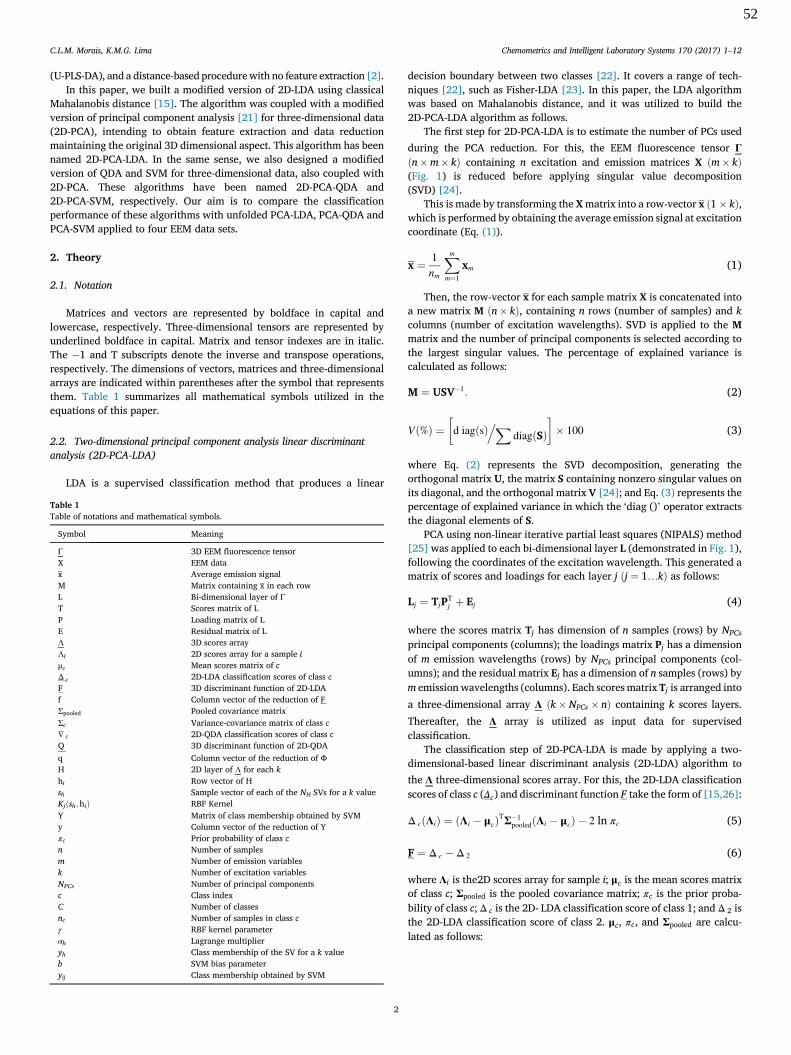
Three-way data has been increasingly used in chemical applications. However, few algorithms are capable ofproperly classifying this type of data maintaining its original dimensions. Unfolding procedures are commonlyemployed to reduce the data dimension and enable its classification using first order algorithms. In this paper,modified versions of two-dimensional principal component analysis with linear discriminant analysis (2D-PCA-LDA), quadratic discriminant analysis (2D-PCA-QDA), and support vector machines (2D-PCA-SVM) have beenproposed to classify three-way chemical data. Applications were performed for two-category classification usingfluorescence excitation emission matrix (EEM) of simulated and three real data sets, in which the performance ofthe proposed algorithms were compared with regular PCA-LDA, PCA-QDA and PCA-SVM using unfolding pro-ceedings. The results show that 2D algorithms had equal or superior classification performance in the four datasets analyzed, thus indicating its ability to classify this type of data.
1. Introduction
The most common way of representing objects for classificationpurposes is in a two-way structure (matrix), where each object of thematrix is represented by a row feature vector (one-dimensional object)[1]. However, some analytical techniques in chemical applicationsgenerate data as a three-way structure, where each object of this struc-ture is represented by a matrix of points (two-dimensional object). Thesematrices are layered one below the other in order to form athree-dimensional array [1], similar to paper sheets in a book.
Applications using three-way chemical data are becoming morecommon as a result of advances in analytical instrumentation andmethods [2]. Examples of three-way chemical data include excitationemission matrix (EEM) fluorescence spectroscopy [3], gas chromatog-raphy coupled to mass spectrometry (LC-MS) [4], ultra-performanceliquid chromatography coupled to mass spectrometry [5], spectral im-aging [6], among others [7]. One of the most utilized techniques is EEMfluorescence spectroscopy due to its relative low-cost, simple instru-mentation, and high sensitivity.
EEM has been used in many different fields such as clinical [8,9], food[10] and environmental analyses [11,12]. However, few algorithms areable to work with this data maintaining its three-dimensional aspect [7].The most known algorithms for classifying EEM data are usually based on
parallel factor analysis (PARAFAC) [13] or Turker3 [14] for datareduction, thereafter being coupled with linear discriminant analysis(LDA) [15], partial least squares discriminant analysis (PLS-DA) [16], orsupport vector machines (SVM) [17] as the classification method.Another strategy to classify EEM data is to unfold the 3D array into amatrix, in which the EEM for each sample is transformed into a rowvector. In this way, first order classification algorithms such as principalcomponent analysis with linear discriminant analysis (PCA-LDA) [18],quadratic discriminant analysis (PCA-QDA) [18] and support vectormachine (PCA-SVM) [19] can be normally applied to the data. However,the unfolding procedure affects the spatial distribution of the data andcould affect its variance structure.
In the context of classifying three-way data, Li et al. [20] proposed theuse of two-dimensional linear discriminant analysis (2D-LDA) as a new al-gorithm for image feature extraction and selection applied in face imageprocessing. This algorithm used the image matrix to compute thebetween-class scatter matrix and the within-class scatter matrix to beemployed in Fisher linear discriminant analysis. As an advantage, it ach-ieved high recognition accuracy and low computation cost [20]. Recently,Silva et al. [2] utilized the 2D-LDA algorithm to classify three-way chemicaldata. They obtained very satisfactory results classifying simulated and realEEM data sets using this algorithm in comparison with PARAFAC-LDA,Tucker3-LDA, unfolded partial least squares discriminant analysis
Chemometrics and Intelligent Laboratory Systems 170 (2017) 1–12
51
(U-PLS-DA), and a distance-based procedurewith no feature extraction [2].In this paper, we built a modified version of 2D-LDA using classical
Mahalanobis distance [15]. The algorithm was coupled with a modifiedversion of principal component analysis [21] for three-dimensional data(2D-PCA), intending to obtain feature extraction and data reductionmaintaining the original 3D dimensional aspect. This algorithm has beennamed 2D-PCA-LDA. In the same sense, we also designed a modifiedversion of QDA and SVM for three-dimensional data, also coupled with2D-PCA. These algorithms have been named 2D-PCA-QDA and2D-PCA-SVM, respectively. Our aim is to compare the classificationperformance of these algorithms with unfolded PCA-LDA, PCA-QDA andPCA-SVM applied to four EEM data sets.
2. Theory
2.1. Notation
Matrices and vectors are represented by boldface in capital andlowercase, respectively. Three-dimensional tensors are represented byunderlined boldface in capital. Matrix and tensor indexes are in italic.The �1 and T subscripts denote the inverse and transpose operations,respectively. The dimensions of vectors, matrices and three-dimensionalarrays are indicated within parentheses after the symbol that representsthem. Table 1 summarizes all mathematical symbols utilized in theequations of this paper.
2.2. Two-dimensional principal component analysis linear discriminantanalysis (2D-PCA-LDA)
LDA is a supervised classification method that produces a linear
decision boundary between two classes [22]. It covers a range of tech-niques [22], such as Fisher-LDA [23]. In this paper, the LDA algorithmwas based on Mahalanobis distance, and it was utilized to build the2D-PCA-LDA algorithm as follows.
The first step for 2D-PCA-LDA is to estimate the number of PCs used
during the PCA reduction. For this, the EEM fluorescence tensor Γðn�m� kÞ containing n excitation and emission matrices X ðm� kÞ(Fig. 1) is reduced before applying singular value decomposition(SVD) [24].
This is made by transforming the Xmatrix into a row-vector x ð1� kÞ,which is performed by obtaining the average emission signal at excitationcoordinate (Eq. (1)).
x ¼ 1nm
Xm
m¼1
xm (1)
Then, the row-vector x for each sample matrix X is concatenated intoa new matrix M ðn� kÞ, containing n rows (number of samples) and kcolumns (number of excitation wavelengths). SVD is applied to the Mmatrix and the number of principal components is selected according tothe largest singular values. The percentage of explained variance iscalculated as follows:
M ¼ USV�1: (2)
Vð%Þ ¼�d iagðsÞ
.XdiagðSÞ
�� 100 (3)
where Eq. (2) represents the SVD decomposition, generating theorthogonal matrix U, the matrix S containing nonzero singular values onits diagonal, and the orthogonal matrix V [24]; and Eq. (3) represents thepercentage of explained variance in which the ‘diag ()’ operator extractsthe diagonal elements of S.
PCA using non-linear iterative partial least squares (NIPALS) method[25] was applied to each bi-dimensional layer L (demonstrated in Fig. 1),following the coordinates of the excitation wavelength. This generated amatrix of scores and loadings for each layer j ðj ¼ 1…kÞ as follows:
Lj ¼ TjPTj þ Ej (4)
where the scores matrix Tj has dimension of n samples (rows) by NPCs
principal components (columns); the loadings matrix Pj has a dimensionof m emission wavelengths (rows) by NPCs principal components (col-umns); and the residual matrix Ej has a dimension of n samples (rows) bym emission wavelengths (columns). Each scores matrix Tj is arranged into
a three-dimensional array Λ ðk� NPCs � nÞ containing k scores layers.
Thereafter, the Λ array is utilized as input data for supervisedclassification.
The classification step of 2D-PCA-LDA is made by applying a two-dimensional-based linear discriminant analysis (2D-LDA) algorithm to
the Λ three-dimensional scores array. For this, the 2D-LDA classificationscores of class c (Δc) and discriminant function F take the form of [15,26]:
where Λi is the2D scores array for sample i; μc is the mean scores matrixof class c; Σpooled is the pooled covariance matrix; πc is the prior proba-bility of class c; Δ c is the 2D- LDA classification score of class 1; and Δ 2 isthe 2D-LDA classification score of class 2. μc, πc, and Σpooled are calcu-lated as follows:
Table 1Table of notations and mathematical symbols.
Symbol Meaning
Γ 3D EEM fluorescence tensorX EEM datax Average emission signalM Matrix containing x in each rowL Bi-dimensional layer of ΓT Scores matrix of LP Loading matrix of LE Residual matrix of LΛ 3D scores arrayΛi 2D scores array for a sample iμc Mean scores matrix of cΔ c 2D-LDA classification scores of class cF 3D discriminant function of 2D-LDAf Column vector of the reduction of FΣpooled Pooled covariance matrixΣc Variance-covariance matrix of class c∇ c 2D-QDA classification scores of class cQ 3D discriminant function of 2D-QDAq Column vector of the reduction of ΦH 2D layer of Λ for each khi Row vector of Hsh Sample vector of each of the NH SVs for a k valueKjðsh;hiÞ RBF KernelY Matrix of class membership obtained by SVMy Column vector of the reduction of Yπc Prior probability of class cn Number of samplesm Number of emission variablesk Number of excitation variablesNPCs Number of principal componentsc Class indexC Number of classesnc Number of samples in class cγ RBF kernel parameterαh Lagrange multiplieryh Class membership of the SV for a k valueb SVM bias parameteryij Class membership obtained by SVM
C.L.M. Morais, K.M.G. Lima Chemometrics and Intelligent Laboratory Systems 170 (2017) 1–12
2
52
μc ¼1nc
Xnc
i¼1
Λi (7)
πc ¼ncnT
(8)
Σpooled ¼1nT
XC
c¼1
ncΣc (9)
where nc is the number of samples in class c; nT is the total number ofsamples in training set; C is the number of classes; and Σc is the variance-covariance matrix of class c defined as:
Σc ¼1
nc � 1
Xnc
i¼1
ðΛi � μcÞðΛi � μcÞT (10)
As Fijw ðn� k� kÞ is also a three-dimensional array, it needs to bereduced in order to have a single element fjw representing each sample forthe algorithm be able to assign a class. This procedure is made using thevalidation set, where j and w positions are determined according to thesmaller distance between F of the validation set and the mean F of its trueclass in the training set. The point (j,w) where this distance is smalleramong all validation samples (as a consequence where the error issmaller) is chosen. Next, j and w are set constant for all samples beinganalyzed, thus F becomes a column vector f ðn� 1Þ. Thus, if the value fi1of a sample i present in f is positive, the sample is assigned as class 1; ifnegative, the sample is assigned as class 2.
2.3. Two-dimensional principal component analysis quadratic discriminantanalysis (2D-PCA-QDA)
QDA is a supervised classification technique very similar to LDA,which also uses Mahalanobis distance [22]. The main difference betweenthem is that QDA calculates the distance to each class using the sample
variance-covariance matrix of each class rather than the pooled covari-ance matrix [22]. This enables QDA to form a separated variance modelfor each class; whereas LDA does not take into account different variancestructures for the two classes [22].
The 2D-PCA reduction used in 2D-PCA-QDA is the same utilized in
2D-PCA-LDA (Fig. 1), where the 3D scores array Λ ðk� NPCs � nÞ is uti-lized for classification. The 2D-QDA classification scores of class c ð∇ cÞand discriminant function Q take the form of [15,26]:
where ∇ 1 and ∇ 2 are the 2D-QDA classification score of class 1 and 2,respectively.
The same procedure is performed to reduce the size of F is made withQijw ðn� k� kÞ, whereQ becomes a column vector q ðn� 1Þ by using thepoint ðj;wÞ selected according to the smaller distance found betweenQ of
the validation set and the meanQ of its true class in the training set. If thevalue qi1 of a sample i present in q is positive, the sample is assigned asclass 1; if negative, the sample is assigned as class 2.
2.4. Two-dimensional principal component analysis support vectormachine (2D-PCA-SVM)
SVM is a powerful supervised classification technique based on binaryclassifiers that work by finding a classification hyperplane which sepa-rates two classes with the largest margin of separation [27]. A keyadvantage of SVM over other classification methods (such as LDA) is thatSVM is capable of classifying non-linearly separable data [27].
The 2D-PCA reduction employed in 2D-PCA-SVM is the same utilizedin both 2D-PCA-LDA and 2D-PCA-QDA algorithms (Fig. 1); and the 3D
scores array Λ was utilized as data input for the 2D-SVM. The 2D-SVMalgorithm was based on a radial basis function (RBF) kernel, which is thesimplest kernel commonly employed using SVM [22]. The kernel is
Fig. 1. Illustration of data processing using 2D-PCA.
C.L.M. Morais, K.M.G. Lima Chemometrics and Intelligent Laboratory Systems 170 (2017) 1–12
3
53
responsible for transforming the data into a feature space and for itsclassification ability [22,28].
Let us assume that the 3D array Λ ðk� NPCs � nÞ is composed of klayers (matrices) H ðn� NPCsÞ having n elements hi representing eachsample i (each row). The RBF kernel Kjðsh;hiÞ is calculated for eachexcitation wavelength j as follows [22]:
Kjðsh;hiÞ ¼ exp�� γ����sh � hi
��j2�
(13)
where j ¼ 1…k; sh is the sample vector of each of the NH support vectors(SVs) in each j; hi ð1� PCsÞ is the scores vector of a sample i for each jexcitation wavelength; and γ is the parameter that determines the widthof the RBF.
The SVM classification rule takes the form of [22]:
yij ¼ sign
XH
h¼1
αhyhKjðsh;hiÞ þ b
!(14)
where αh is the Lagrange multiplier; yh is the class membership (±1) ofthe corresponding SV at each j excitation wavelength; and b is thebias parameter.
The calculation of Kjðsh;hiÞ and yij is made for all k excitationwavelengths. Consequently, a matrix of yij elements is created (Yðn� kÞ.Similar to 2D-PCA-LDA and 2D-PCA-QDA, the best k wavelength from Yis selected according to the lowest error in validation set. As a result, acolumn vector y ðn� 1Þ is created having the assigned class indexes foreach sample (each row).
3. Experimental
3.1. Software
Data processing was performed using MATLAB® R2012b software
(MathWorks, Inc., USA). All chemometric algorithms were applied usinglab-made codes in the MATLAB environment. SVM algorithm was runusing default γ parameter equal to 1. All data were mean centeredbefore analysis.
3.2. Simulated data set
Simulated EEMs (data set 1) were built based on normal distributionfunctions having mean (μ) and standard-deviation (σ) parametersrandomly generated inside the range of 0–3 and 0.050–0.150, respec-tively. Each EEM had a size of 301 rows (representing emission wave-lengths) and 12 columns (representing excitation wavelengths). Theexcitation wavelengths were set from 320 to 380 nm (resolution of 8 nm);and emission wavelengths were from 410 to 530 nm (resolution of0.33 nm). A total of 60 EEMs (n ¼ 60) were generated with each onerepresenting a sample. Class 1 contained the first 30 EEMs (totalμ ¼ 28.753; and total σ ¼ 2.949); and class 2 contained the other 30remaining EEMs (total μ ¼ 22.213; and total σ ¼ 2.911). Table 2 showsthe μ and σ parameters utilized to generate each EEM.
3.3. Cod fillets data set
EEM fluorescence data of cod (Gadus morhua) fillets were utilized asdata set 2. This data is publicly available at http://www.models.life.ku.dk/datasets by Andersen et al. [29]. The cod samples were from a sin-gle catch caught in February 1999 in the Barents Sea. The cod wascold-stored in a modified atmosphere (40% CO2/40% N2/20% O2) at2 �C for up to 21 days. Aqueous extracts were made homogenizing 25 g offish muscle with 75 mL of water. The pH was reduced to 5.2 and themixture was heated at 70 �C, cooled to room temperature and filtered toremove precipitated proteins. The extracts were measured at 22 �C in10 � 10 nm thermostatic quartz cuvette on a Perkin-Elmer LS50B spec-trofluorimeter [29]. The data was preprocessed by removing emissionsfrom 270 to 280 nm in order to reduce Rayleigh scatter andmissing values.
Table 2Mean (μ) and standard-deviation (σ) used for construct data set 1 (simulated data) based onan underlying normal distribution.
Table 3Number of samples in training, validation and test sets.
Class Number of samples
Training Validation Test
Data set 1 1 20 5 52 20 5 5Total 40 10 10
Data set 2 1 44 9 102 29 6 7Total 73 15 17
Data set 3 1 53 12 122 52 11 11Total 105 23 23
Data set 4 1 52 11 112 52 11 11Total 104 22 22
Table 4Statistical quality parameters. TP stands for true positive; FP for false positive; TN for truenegative; and FN for false negative. ε1 is the number of misclassified samples in class 1; ε2 isthe number of misclassified samples in class 2; and N is the total number of samples.
C.L.M. Morais, K.M.G. Lima Chemometrics and Intelligent Laboratory Systems 170 (2017) 1–12
4
54
A total of 105 samples (n ¼ 105) were divided into two classes.Class 1 contained 63 samples of cod stored up to 1 week (0–7 days);and class 2 contained 42 samples of cod stored from more than 14 days(14–21 days). The EEM for each sample had a size of 331 rows(emission wavelengths) and 13 columns (excitation wavelengths). Theexcitation wavelengths were from 250 to 370 nm (resolution of10 nm); and emission wavelengths were from 270 to 600 nm (reso-lution of 1 nm).
3.4. Colorectal cancer data set
EEM fluorescence plasma data of patients in healthy conditions (nofindings at endoscopy) and with verified colorectal cancer (CRC) wereutilized to build data set 3. This data is publicly available at http://www.models.life.ku.dk/datasets by Lawaetz et al. [30]. The samples of humanplasma (sodium citrate anticoagulant) were defrosted on wet ice (0 �C)for approximately 40 min, and measured as fast as possible after thawing
Fig. 2. Average EEM of: class 1 (a) and 2 (b) in data set 1; class 1 (c) and 2 (d) in data set 2; class 1 (e) and 2 (f) in data set 3; and class 1 (g) and 2 (h) in data set 4.
C.L.M. Morais, K.M.G. Lima Chemometrics and Intelligent Laboratory Systems 170 (2017) 1–12
5
55
in an FS920 spectrometer (Edinburgh Instruments) with double mono-chromators and a R928P red sensitive photomultiplier (Hamamatsu) in acooled detector house [30]. The acquired EEM data were preprocessed byremoving Rayleigh scatter and second order fluorescence.
A total of 151 EEMs (n ¼ 151) were divided into class 1 (77 EEMs ofhealthy patients) and class 2 (74 EEMs of patients with CRC). Each EEMhad a size of 301 rows (emission wavelengths) and 41 columns (excita-tion wavelengths). The excitation wavelengths were from 250 to 450 nm(resolution of 5 nm), and emission wavelengths were from 300 to 600 nm(resolution of 1 nm).
3.5. Adenomas versus colorectal cancer data set
Data set 4 was built using EEM fluorescence plasma data of patientswith pathologically verified adenomas [31] and patients with verifiedCRC. This data is also publicly available at http://www.models.life.ku.dk/datasets by Lawaetz et al. [30]. The EEMs of human plasma sam-ples (sodium citrate anticoagulant) were acquired at higher excitation(385–425 nm, resolution of 5 nm) and emission (585–680 nm, resolutionof 1 nm) wavelengths in the same instrument as data set 3. The samples
were also measured as quickly as possible after thawing [30].The acquired EEMs (n ¼ 148) were divided in two classes: class 1
having 74 EEMs of patients with adenomas (control group); and class 2having 74 EEMs of patients with CRC. Each EEM had a size of 96 rows(emission wavelengths) and 9 columns (excitation wavelengths).
3.6. Sample selection
The samples in each data set were divided into training (~70%),validation (~15%) and test (~15%) sets using the Kennard-Stone sam-pling selection algorithm [32]. The algorithm was firstly applied to theunfolded data and the same samples' indexes for training, validation andtest sets were implemented into the 2D algorithms. The numbers ofsamples in training, validation and test sets for each data set are shownin Table 3.
3.7. Statistical validation
The performances of both unfolded and 2D algorithms were evalu-ated according to the following quality parameters: percentage of correct
Fig. 3. Singular value of unfolded and 2D EEM data matrices of data set 1 (a), data set 2 (b), data set 3 (c), and data set 4 (d). Inset: singular value zooming of 2D EEM data.
Table 5Explained variance (%) of the first 15 PCs obtained by the unfolded and 2D PCA models for data sets 1–4.
C.L.M. Morais, K.M.G. Lima Chemometrics and Intelligent Laboratory Systems 170 (2017) 1–12
6
56
classification (CC%), accuracy (AC), sensitivity (SENS), specificity(SPEC), positive predictive value (PPV), negative predictive value (NPV),positive likelihood ratio (LRþ), negative likelihood ratio (LR-), F-Score,and G-Score [18,33,34]. Table 4 shows the equations utilized to calculateeach one of these parameters.
The CC% represents the number of samples correctly classified aspositive; the accuracy represents the total number of samples correctlyclassified considering true and false negatives; the sensitivity measuresthe proportion of positives that are correctly identified; the specificitymeasures the proportion of negatives that are correctly identified; thePPV shows how many of the test positives are true positives; the NPVshows how many of the test negatives are true negatives; theLR þ represents the ratio between the probability of predicting a sampleas positive when it is truly positive, and the probability of predicting asample as positive when it is actually negative; the LR-represents the
ratio between the probability of predicting a sample as negative when itis actually positive, and the probability of predicting a sample as negativewhen it is truly negative; the F-Score measures the performance of themodel considering imbalanced data; and G-Score measures the perfor-mance of the model not accounting for the size of the classes [18,34].
4. Results
The four fluorescence data sets analyzed were built for two-categorydiscriminatory analysis as follows: (1) simulated fluorescence spectragenerated with different means and standard-deviation using normaldistribution; (2) spectra of cod fillets stored at 2 �C until one week (0–7days) and stored from more than 14 days (14–21 days); (3) spectra ofhealthy control and subjects with colorectal cancer (CRC) acquired inplasma; and (4) spectra of plasma of control group with pathologicalverified adenomas and subjects with CRC. The excitation and emissionwavelengths varied among the data sets as follows: 320–380 nm
Fig. 4. 2D-PCA scores on: PC 1 (a) and PC 2 (b) in data set 1; PC 1 (c) and PC 2 (d) in dataset 2; PC 1 (e) and PC 2 (f) in data set 3; and PC1 (g) and PC2 (h) in data set 4. Ex. standsfor excitation wavelength.
Fig. 5. 2D-PCA loadings on: PC 1 (a) and PC 2 (b) in data set 1; PC 1 (c) and PC 2 (d) indata set 2; PC 1 (e) and PC 2 (f) in data set 3; and PC1 (g) and PC2 (h) in data set 4. Em.stands for emission and Ex. for excitation wavelength.
C.L.M. Morais, K.M.G. Lima Chemometrics and Intelligent Laboratory Systems 170 (2017) 1–12
7
57
(excitation) and 410–530 nm (emission) in data set 1; 250–370 nm(excitation) and 270–600 nm (emission) in dataset 2; 250–450 nm(excitation) and 300–600 nm (emission) in dataset 3; and 385–425 nm(excitation) and 585–680 nm (emission) in data set 4. Fig. 2 shows theaverage EEM for each class in data sets 1–4. Visual inspection allowsidentifying some distinguishing features among the EEM in each data set.Significant differences between the mean of categories (P < 0.01) werefound for data sets 2 and 3.
2D-PCA was initially applied to the data in order to reduce the EEMmatrices into few principal components (PCs) accounting to the most ofthe original explained variance. This removes possible noise andredundant information from the original data, and speeds up computa-tional analysis. The number of PCs was selected according to the highestsingular values obtaining using the SVD algorithm. The singular valuesfor each data set using unfolded and 2D matrices are shown in Fig. 3.
The singular value profiles using the unfolded and 2D matrices weresimilar to each other; however, the 2D singular values had much lowerintensity. The number of PCs selected for each data set was equal to 10 indata sets 1–3, and 8 in data set 4. The number of selected PCs for bothmethods was the same in order to maintain consistency for comparingthe unfolded and 2D models. The percentage of explained variance forthe first 15 PCs in each data set is shown in Table 5.
As 2D-PCA algorithm was performed in excitation wavelength di-rection, the maximum number of PCs is equal to the number of excitationvariables. Therefore, the algorithm does not reach 15 PCs in data sets 1, 2and 4, since there are only 12, 13 and 9 excitation wavelengths in thesedata sets, respectively. The scores and loadings generated in 2D-PCA aretwo-dimensional, where each PC has its own scores and loadingsmatrices. Each scores matrix has dimension of n samples by k excitationwavelengths; and each loadings matrix has dimension of m emission
Fig. 6. Unfolded PCA scores and loadings for EEM data matrices. (a) scores and (b) loadings on PC1 and PC2 for data set 1; (c) scores and (d) loadings on PC1 and PC2 for data set 2; (e)scores and (f) loadings on PC1 and PC2 for data set 3; and (g) scores and (h) loadings on PC1 and PC2 for data set 4. Em. stands for emission and Ex. for excitation wavelength. Loadingsprofiles were folded back into the original 2D EEM dimension. A 95% confidence ellipse is shown in each scores plot.
C.L.M. Morais, K.M.G. Lima Chemometrics and Intelligent Laboratory Systems 170 (2017) 1–12
8
58
wavelengths by k excitation wavelengths. The two-dimensional scoresand loadings matrices on the 1st and 2nd PCs are shown in Figs. 4 and 5,respectively.
The unfolded scores and loadings obtaining by PCA for data sets 1–4are shown in Fig. 6. The difference between the 2D and unfolded profilesof the scores and loadings matrices is clearly shown.
In order to classify the two categories present in each data set, regularand two-dimensional LDA, QDA and SVMwere applied to the PCA scoresusing unfolded and 2D mode, respectively. The correct classification (CC%) rates obtained in training, validation and test sets are shownin Table 6.
In order to evaluate the prediction performance of both unfolded and2D classification algorithms, the statistical quality parameters of accu-racy (AC), sensitivity (SENS), specificity (SPEC), positive predictive value(PPV), negative predictive value (NPV), positive likelihood ratio (LRþ),negative likelihood ratio (LR-), F-Score and G-Scores were calculatedusing the test set (Table 7). These parameters provide more reliable in-formation about the classification performance of each algorithm.
In data set 1 and 4, the best classification performance was obtainedby both PCA-SVM and 2D-PCA-SVM algorithms (G-Score¼ 80.0% in dataset 1; and G-Score ¼ 81.8% in data set 4). In addition, the 2D-PCA-SVMalgorithm had the best performance in data set 2 and 3 (G-Score¼ 88.2%and 72.0%, respectively).
5. Discussion
5.1. Simulated data set
Despite having no chemical significance, simulated data is often usedas a primary data set to evaluate discriminatory performance of classi-fication algorithms [2,22]. We create an EEM simulated data set (data set1) based on a normal distribution having different means and standard-
deviations randomly generated for each class.The effect of 2D-PCA reduction in this data set was very significant, in
which the first PC had almost double the explained variance than usingregular PCA with unfolded matrices (Table 5). This also reflected thecumulative explained variance in the first 10 selected PCs, in which the2D-PCA algorithm had a 45.73% higher explained variance (99.24%)than unfolded PCA (68.10%).
The two-dimensional PCA scores (Fig. 4a and b) show no clear sep-aration between classes 1 and 2, although a highly disperse profile isobserved, especially in PC1. On the other hand, the unfolded PCA scoreson the 1st and 2nd PCs (Fig. 6a) show an entirely superimposed profile, inwhich no differences between the classes' scores are observed. The 2D-PCA loadings on the 1st and 2nd PCs (Fig. 5a and b) are completelydifferent from the unfolded PCA. In the 2D-PCA, the loadings profile isvery dispersed among the excitation and emission wavelengths, where nomajor area has higher coefficients; in contrast, the PCA loadings obtainedfrom the unfolded matrices (Fig. 6b) have higher coefficients along theexcitation wavelength close to 270 nm on both PC1 and PC2.
The PCA-QDA algorithm had the best correct classification (CC%)rate in training, validation and test set (100%); however, its classificationperformance was highly affected by a possible overfitting that reflectedpoor accuracy, sensitivity and specificity in Table 6. The 100% PPV foundindicates the model's high ability to identify true positives; however, thelower NPV (0.0%) indicates that the model is not able to identify falsenegatives. This made the specificity of the model equal to 0.0%, gener-ating a G-Score of 0%, thus indicating no classification ability. On theother hand, despite 2D-PCA-QDA had a poor correct classification rate,its classification performance was not affected by overfitting. The G-Score of 65.2% indicates that this algorithmwas more efficient than PCA-QDA, PCA-LDA and 2D-PCA-LDA algorithms, which had equal classifi-cation ability (G-Score ¼ 60.0%).
The best classification performance for this data set was obtainedusing both PCA-SVM and 2D-PCA-SVM algorithms (G-Score ¼ 80.0%).SVM classifier usually achieves better classification rates than LDA andQDA, since SVM is able to create a more complex decision boundarybetween the classes, enabling classification of non-linearly separabledata [22,27].
5.2. Cod fillet data set
Determination of fish freshness is an important parameter to assessquality. Fish retains their original characteristics closer to the harvest[35]. EEM fluorescence spectra of relatively new cod samples stored at2 �C up to 1 week (class 1) and relatively old cod samples stored at thesame temperature from more than 14 days (class 2) were analyzed inorder to create a discriminant model between these two classes (data set2). The time distinction between the classes provokes changes in thesamples, such as microbiological growth and alterations in biochemical,chemical and physical properties [35].
The EEM mean profile for classes 1 and 2 are very similar to eachother (Fig. 2c and d), where a very intense band is observed close to theexcitation wavelength of 300 nm and emission of 370 nm; and smallerbands are present between 300 and 360 nm (excitation) and 370–400 nm(emission) wavelengths.
Ten principal components were selected in PCA with cumulativeexplained variance of 94.04% using unfolded PCA; and 99.65% using 2D-PCA. 2D-PCA scores on the 1st and 2nd PCs (Fig. 4c and d) show nodiscriminant profile between the two classes, since the scores are verymixed. On the other hand, unfolded PCA scores on the 1st PC show somedistinction between fresh and aged samples along its axis (Fig. 6c). Theunfolded PCA loadings on PC1 and PC2 (Fig. 6d) show higher coefficientsin the same region as the most intense band in the EEM data. The 2D-PCAloadings on the 1st and 2nd PCs have more distributed coefficientsamong emission wavelengths between 370 and 400 nm (Fig. 5c and d),including regions with smaller bands.
The correct classification (CC%) rate using unfolded PCA-LDA and
Table 6Correct classification (CC%) for training, validation and test sets obtained using unfoldedand 2D classification algorithms in data sets 1–4.
C.L.M. Morais, K.M.G. Lima Chemometrics and Intelligent Laboratory Systems 170 (2017) 1–12
9
59
PCA-QDA algorithm were higher than using 2D-PCA-LDA and 2D-PCA-QDA, despite the 2D algorithms having a better fit in the training set(Table 6). For SVM-based algorithm, 2D-PCA-SVM had equally correctclassification in the training set (100%), and the best CC% in validationand test set, with an increase of 16.6% and 15.3%, respectively. Thequality parameters of Table 7 also show this same trend, in whichunfolded PCA-LDA and PCA-QDA had better prediction performancethan 2D-PCA-LDA and 2D-PCA-QDA algorithms. Perhaps 2D-PCA incor-porated more noise or no significant variations from data set 2 to themodel, as its loadings incorporate larger areas of the EEM data having nosignificant bands, which could reduce the performance of 2D-LDA and2D-QDA algorithms. As SVM have larger margins of separation betweenthe two classes, its classifier has more stability so that small disturbancesor noise do not cause misclassification [27]. Thus, 2D-PCA-SVM had thebest classification performance among the algorithms tested for this dataset with a G-Score of 88.2%. In fact, this model had the best classificationperformance among all datasets as well, with accuracy, sensitivity,specificity, PPV, NPV, F-Score and G-score all equal to 88.2%; and it hadthe largest values of LRþ (7.5) and LR- (0.1).
5.3. Colorectal cancer data set
Colorectal cancer (CRC) is one of the major causes of cancer-relateddeath in western countries [36], and its identification is very laboriousand invasive. In this sense, fluorescence technique allied with chemo-metric tools have been used as a less-invasive and alternative method forcancer identification without complex technology or elevated costs [30].Fluorescence spectroscopy has great potential due its high sensitivity andits interaction with many important plasma compounds [30]. Data set 3was composed of fluorescence EEMs of plasma of patients in healthyconditions (class 1) and diagnosed with CRC (classes 2). Both EEM datafor class 1 and 2 are very similar to each other (Fig. 2e and f); however,class 2 has a little more intense mean intensity. The most intense bandsare in the region of 250–350 nm (excitation) and 300–400 nm (emission)
wavelengths. The ultraviolet area is dominated by excitation and emis-sion of aromatic tyrosine and tryptophanamino acids, for this reason, itcorresponds to fluorescence of proteins; whereas the visible area ischaracterized by excitation and emissions of vitamins and cofactors [30].
Ten PCs were selected during PCA, accounting for 92.83% (unfolded)and 98.26% (2D) of cumulative explained variance. Both 2D (Fig. 4e andf) and unfolded (Fig. 6e) PCA scores are very superimposed, with no clearseparation between the classes being observed. The loadings profile of2D-PCA on the 1st and 2nd PCs (Fig. 5e and f) indicates higher co-efficients in three different areas: (i) between 350 and 450 nm (excita-tion) and 450–600 nm (emission) wavelengths; (ii) among the excitationwavelength at 330 nm; and (iii) between 250 and 330 nm (excitation)and 300–400 nm (emission) wavelengths. All these regions are related tofluorescence bands on the original EEM data in the following order ofintensity: (iii) > (ii) > (i). In the unfolded PCA, the loadings on the 1st PChad higher coefficients in region (iii), and the loadings on the 2nd PC inregions (ii) and (iii). The CC% rate for data set 3 was higher using 2Dalgorithms (Table 6), where all three algorithms (2D-PCA-LDA, 2D-PCA-QDA, 2D-PCA-SVM) had higher CC% on the test set. Additionally, pre-diction performance (Table 7) was higher using 2D algorithms, with theexception of 2D-PCA-LDA.
Poor fitting in the training set of 2D-PCA-LDA (CC% ¼ 60.0%)contributed to the presence of more false negatives, reducing its accuracyto 56.2% and PPV to 43.5%. This directly affected the sensitivity andspecificity of the model, and consequently the G-Score (57.0%). Allunfolded algorithms had the same performance (G-Score ¼ 60.9%),which was probably caused by both classes having similar variancestructures. The similarities between F-Score and G-Score also corroboratethis hypothesis, since the values were equal despite classes havingdifferent sizes (class 1 ¼ 77 samples, and class 2 ¼ 74 samples). Mostlikely the prior probability term πk in LDA and QDA equations (Eq. (5)and Eq. (11), respectively) had low influence on the classification score.
The best classification performance was found using 2D-PCA-SVM (G-Score ¼ 72.0%), with accuracy (71.7%), sensitivity (69.2%) and
Table 7Statistical quality parameters obtained using unfolded and 2D classification algorithms in data sets 1–4. Accuracy (AC), sensitivity (SENS), specificity (SPEC), positive predictive value (PPV),negative predictive value (NPV), F-Score, and G-Score are expressed in %. The model with best classification performance in each data set is highlighted in bold.
Data set AC SENS SPEC PPV NPV LRþ LR- F-Score G-Score
C.L.M. Morais, K.M.G. Lima Chemometrics and Intelligent Laboratory Systems 170 (2017) 1–12
10
60
specificity (75.0%) being respectively 17.7%, 13.6% and 23.2% higherthan unfolded PCA-SVM. The predictive performance of 2D-PCA-SVM iscomparable to known biomarkers for CRC in serum such as carcinoem-bryonic antigen (CEA), which has sensitivity and specificity of 34% and93%, respectively [30].
5.4. Adenomas versus CRC data set
Adenomas are tumors that are not cancer, and start in gland-like cellsof the epithelial tissue [37]. Adenomas of the colon are estimated to bepresent in 20–53% of the U.S. population older than 50 years age [38].They are categorized as either conventional adenomas or sessile serratedpolyps, and are known as precursors in the majority of cases of CRC [38].Distinguishing them from CRC is an important task to perform appro-priate treatment and to reduce the risk of cancer. In data set 4, EEMfluorescence plasma spectra of patients with adenomas (class 1) and CRC(class 2) were analyzed. The EEM data for class 1 and 2 (Fig. 2g and h)was collected from a higher excitation wavelength than previous datasets, and its format is quite distinguishing. The higher wavelengthsprovide information about porphyrin fluorescence, which could berelated to cancer, since a high concentration of this compound has beendetected in blood from patients with cancer [30]. The fluorescence ofporphyrin is in the region of 405 nm (excitation)/610 nm (emission), and400 nm (excitation)/620 nm (emission) [30]. However, similar profilesare observed among the EEM for both classes, with slight differencesclose to the emission wavelength of 585 nm.
PCA reduced the data into 8 selected PCs with cumulative explainedvariance of 97.90% and 99.97% for unfolded and 2D algorithm,respectively. The 2D-PCA scores on the 1st PC (Fig. 4g) show some class 2excitation variables clearly separated from the rest along 390–420 nm;while PC2 (Fig. 4h) has no clear discriminatory profile. The unfolded PCAscores on the 1st and 2nd PCs (Fig. 6g) show that they are completelysuperimposed, where only class 2 is visible. The 2D and unfolded PCAloadings profiles on the 1st and 2nd PCs are similar, where the loadingson PC1 have similar shape to the original EEM data; and the loadings onPC2 has a region of higher coefficients between 405 and 420 nm (exci-tation) and 585 m (emission) wavelengths (which was the area with themain observable difference between the class 1 and 2). These regionsseem not related to the presence of porphyrin.
The CC% rate indicates better fitting with the training set using 2Dalgorithms, however the CC% for the test set was higher using PCA-QDAthan 2D-PCA-QDA (Table 6). Furthermore, an equal CC% for test set(81.8%) is obtained using PCA-SVM and 2D-PCA-SVM algorithms. Thissame trend is observed in the quality parameters of Table 7, where PCA-SVM and 2D-PCA-SVM have the best performance with equal figures ofmerit. The values of sensitivity and specificity of 81.8% found by thesemodels are the second largest among all tested data sets, and seems to besatisfactory for this type of application as the CEA biomarker has sensi-tivity/specificity of 34/93% [30].
6. Conclusion
This paper demonstrated the use of 2D algorithms (2D-PCA-LDA, 2D-PCA-QDA and 2D-PCA-SVM) as feature extraction and classification toolsfor EEM fluorescence data. Four EEM data sets were investigated, withone simulated and three real data ((i) discrimination of cod storage time;(ii) identification of patients with colorectal cancer; and (iii) differenti-ation of patients with adenomas and colorectal cancer). These data setswere classified using unfolded (PCA-LDA, PCA-QDA, and PCA-SVM) and2D algorithms; and their performances were compared according toprediction quality parameters. The 2D-PCA-SVM algorithm had equal orsuperior classification performance for all applications of two-categorydiscrimination in comparison with unfolded methods. In addition, ad-vantages of using 2D-PCA-LDA and 2D-PCA-QDA rather than unfoldedPCA-LDA or PCA-QDA were observed for data sets 1, 3 and 4; where oneof these 2D algorithms had superior classification performance to its
unfolded version. These findings indicate that these 2D algorithms havepromising potential to be employed in classification applications usingEEM fluorescence spectroscopy, or even other types of data based onthree-way structures.
Acknowledgements
Camilo L.M. Morais would like to acknowledge PPGQ/UFRN andCAPES for financial support. K.M.G. Lima acknowledges CNPq (grant305962/2014-4) for financial support.
References
[1] D. Porro-Mu~noz, R.P.W. Duin, I. Talavera, M. Orozco-Alzate, Classification of three-way data by the dissimilarity representation, Signal Process. 91 (2011) 2520–2529.
[2] A.C. da Silva, S.F.C. Soares, M. Insausti, R.K.H. Galv~ao, B.S.F. Band, M.C.U. deAraújo, Two-dimensional linear discriminant analysis for classification of three-waychemical data, Anal. Chim. Acta 938 (2016) 53–62.
[3] R. Bro, M. Vidal, EEMizer: automated modeling of fluorescence EEM data, Chemom.Intell. Lab. Syst. 106 (2011) 86–92.
[4] M. Vosough, A. Salemi, Second-order standard addition for deconvolution andquantification of fatty acids of fish oil using GC-MS, Talanta 73 (2007) 30–36.
[5] K.M.G. Lima, C. Bedia, R. Tauler, A non-target chemometric strategy applied toUPLC-MS sphingolipid analysis of a cell line exposed to chlorpyrifos pesticide: afeasibility study, Microchem. J. 117 (2014) 255–261.
[6] D.E. Halliwell, C.L.M. Morais, K.M.G. Lima, J. Trevisan, M.R.F. Siggel-King,T. Craig, J. Ingham, D.S. Martin, K.A. Heys, M. Kyrgiou, A. Mitra, E. Paraskevaidis,G. Theophilou, P.L. Martin-Hirsch, A. Cricenti, M. Luce, P. Weightman, F.L. Martin,Imaging cervical cytology with scanning near-field optical microscopy (SNOM)coupled with an IR-FEL, Sci. Rep. 6 (2016) 29494.
[7] V. G�omez, M.P. Callao, Analytical applications of second-order calibration methods,Anal. Chim. Acta 627 (2008) 169–183.
[8] E. Koller, O. Quehenberger, G. Jürgens, O.S. Wolfbeis, H. Esterbauer, Investigationof human plasma low density lipoprotein by three-dimensional fluorescencespectroscopy, FEBS Lett. 198 (1986) 229–234.
[9] A, C. de O. Neves, R. Tauler, K.M.G. de Lima, Area correlation constraint for theMCR-ALS quantification of cholesterol using EEM fluorescence data: a newapproach, Anal. Chim. Acta 937 (2016) 21–28.
[10] J. Christensen, L. Nørgaard, R. Bro, S.B. Engelsen, Multivariate autofluorescence ofintact food systems, Chem. Rev. 106 (2006) 1979–1994.
[11] C.A. Stedmon, S. Markager, R. Bro, Tracing dissolved organic matter in aquaticenvironments using a new approach to fluorescence spectroscopy, Mar. Chem. 82(2003) 239–254.
[12] G.J. Hall, J.E. Kenny, Estuarine water classification using EEM spectroscopy andPARAFAC-SIMCA, Anal. Chim. Acta 581 (2007) 118–124.
[13] R. Bro, PARAFAC. Tutorial and applications, Chemom. Intell. Lab. Syst. 38 (1997)149–171.
[14] L.R. Tucker, Some mathematical notes on three-mode factor analysis,Psychometrika 31 (1966) 279–311.
[15] W. Wu, Y. Mallet, B. Walczak, W. Penninckx, D.L. Massart, S. Heuerding, F. Erni,Comparison of regularized discriminant analysis, linear discriminant analysis andquadratic discriminant analysis, applied to NIR data, Anal. Chim. Acta 329 (1996)257–265.
[16] A. Kalivodov�a, K. Hron, P. Filzmoser, L. Najdekr, H. Jane�ckov�a, T. Adam, PLS-DAfor compositional data with application to metabolomics, J. Chemom. 29 (2015)21–28.
[17] C. Cortes, V. Vapnik, Support-vector networks, Mach. Learn 20 (1995) 273–297.[18] L.F.S. Siqueira, R.F. Araújo Júnior, A.A. de Araújo, C.L.M. Morais, K.M.G. Lima, LDA
vs. QDA for FT-MIR prostate cancer tissue classification, Chemom. Intell. Lab. Syst.162 (2017) 123–129.
[19] E. Gumus, N. Kilic, A. Sertbas, O.N. Ucan, Evaluation of face recognition techniquesusing PCA, wavelets and SVM, Expert Syst. Appl. 37 (2010) 6404–6408.
[20] M. Li, B. Yuan, 2D-LDA: a statistical linear discriminant analysis for image matrix,Pattern Recognit. Lett. 26 (2005) 527–532.
[21] H. Abdi, L. Williams, Principal component analysis, Wiley Interdiscip. Rev. Comput.Stat. 2 (2010) 433–459.
[22] S.J. Dixon, R.G. Brereton, Comparison of performance of five common classifiersrepresented as boundary methods: euclidean distance to centroids, lineardiscriminant analysis, quadratic discriminant analysis, learning vector quantizationand support vector machines, as dependent on, Chemom. Intell. Lab. Syst. 95(2009) 1–17.
[23] J. Yang, Z. Jin, J.Y. Yang, D. Zhang, A.F. Frangi, Essence of kernel Fisherdiscriminant: KPCA plus LDA, Pattern Recognit. 37 (2004) 2097–2100.
[24] R. Bro, A.K. Smilde, Principal component analysis, Anal. Methods 6 (2014)2812–2831.
[25] P. Geladi, B.R. Kowalski, Partial least-squares regression: a tutorial, Anal. Chim.Acta 185 (1986) 1–17.
[26] T. Naes, T. Isaksson, T. Fearn, T. Davies, A User-friendly Guide to MultivariateCalibration and Classification, NIR Publications, 2002.
[27] P. De Boves Harrington, Support vector machine classification trees, Anal. Chem. 87(2015) 11065–11071.
C.L.M. Morais, K.M.G. Lima Chemometrics and Intelligent Laboratory Systems 170 (2017) 1–12
11
61
[28] J. Luts, F. Ojeda, R. Van de Plas Raf, B. De Moor, S. Van Huffel, J.A.K. Suykens,A tutorial on support vector machine-based methods for classification problems inchemometrics, Anal. Chim. Acta 665 (2010) 129–145.
[29] C.M. Andersen, R. Bro, Practical aspects of PARAFAC modeling of fluorescenceexcitation-emission data, J. Chemom. 17 (2003) 200–215.
[30] A.J. Lawaetz, R. Bro, M. Kamstrup-Nielsen, I.J. Christensen, L.N. Jørgensen,H.J. Nielsen, Fluorescence spectroscopy as a potential metabonomic tool for earlydetection of colorectal cancer, Metabolomics 8 (2012) 111–121.
[31] A.F. Lomholt, G. Høyer-Hansen, H.J. Nielsen, I.J. Christensen, Intact and cleavedforms of the urokinase receptor enhance discrimination of cancer from non-malignant conditions in patients presenting with symptoms related to colorectalcancer, Br. J. Cancer 101 (2009) 992–997.
[33] L. de Carvalho, C.L.M. de Morais, K.M. de Lima, L.C. Cunha Junior,P.A.M. Nascimento, J. de Faria, G.A. Teixeira, Determination of the geographical
origin and ethanol content of Brazilian sugarcane spirit using near-infraredspectroscopy coupled with discriminant analysis, Anal. Methods 8 (2016)5658–5666.
[34] K.S. Parikh, T.P. Shah, Support vector machine – a large margin classifier todiagnose skin illnesses, Procedia Technol. 23 (2016) 369–375.
[35] H. Nilsen, M. Esaiassen, K. Heia, F. Sigernes, Visible/Near-Infrared spectroscopy: anew tool for the evaluation of fish freshness? J. Food Sci. 67 (2002) 1821–1826.
[36] B.-Q. Li, T. Huang, L. Liu, Y.-D. Cai, K.-C. Chou, Identification of colorectal cancerrelated genes with mRMR and shortest path in protein-protein interaction network,PLoS One 7 (2012), e33393.
[37] National Cancer Institute, NCI Dictionary of Cancer Terms, (n.d.). https://www.cancer.gov/publications/dictionaries/cancer-terms?cdrid¼46217 (accessed March5, 2017).