UNIVERSIT P A U - uni-passau.de

P UNIVERSITaT PASSAUFakult�at f�ur Mathematik und Informatik aDissertation

The Mechanical Parallelization of Loop NestsContaining while LoopsAuthor:Martin GrieblAdvisor:Prof. Christian Lengauer Ph.D.

October 15, 1996

AcknowledgmentsNobody can write a thesis without help form others, and it is usually impossible to expressone's gratitude for this immense amount of help. The least I can do is to devote the �rstpages of my thesis to all these wonderful people, and thank them all for their precious supportand individual help.I want to mention some people explicitly, even knowing that my list must be inclomplete.First of all, I want to thank Professor Christian Lengauer who has been an excellentadvisor to me. Thank you for my position, for your liberality concerning working modes, foruncountably many fruitful discussions with you (o�cial and private), for your indefatigabilityin improving my English, for multiple detailed proof readings of this thesis, for always havingtime for my problems, ...; short, thank you for having been a real \Doktorvater", which, tome, is more than an advisor.In addition, I am grateful to Professor Paul Feautrier: thank you that you have acceptedto review this thesis, and took the time to give me detailed comments on my draft of thisthesis.I also want to thank Professor P. Kleinschmidt, Professor F.-J. Brandenburg and ProfessorW. Hahn for having agreed to being my examiners and for their helpfulness. Furthermore, Iwould like to thank Professor N. Schwartz who always helps at the formal aspects on the wayto a Ph.D.However, there are also helpful persons outside of my dissertation committee. First ofall, I want to thank my French colleague and friend Jean-Fran�cois Collard. Thank you foryour cooperation already at the beginning of this thesis, when we did not yet know eachother. Because of your open-minded way, we succeeded in working together instead of beingcompetitors. This led to many fruitful discussions and a deep friendship. Thanks a lot forthat.Furthermore, I would like to thank the members of the Lehrstuhl f�ur Programmierung forthe good working climate and for some helpful hints, and esp. Christoph Herrmann for hisexcellent proof reading. In addition, there is another member of the group I want to mentionspeci�cally: Ulrike Lechner. I would call her \the good soul of our group". Thank you forsharing the o�ce and some work, and for the wonderful climate in our o�ce, not only due toyour owers.A-pro-pos climate: one of the most agreeable teams I have ever been part of is the LooPoteam. The students in this team have been a continuous source of energy and encouragementto me. Numerous discussions helped me understand the problems in the various facets ofloop parallelization. I am grateful to Andreas Dischinger, Peter Faber, Robert G�unz, HaraldKeimer, Radko Kubias, Wolfgang Meisl, Frank Schuler, Martina Schumergruber, Sabine Wet-zel, Christian Wieninger and Alexander W�ust. A speci�c thank is due to Nils Ellmenreich:

thank you, for being a co-leader of LooPo, and still more for your unbounded helpfulness andfor your friendship.Right, there is one name missing in the LooPo team: Max Geigl. You can be sure that Ihave not forgotten you, M�ax; I just want to thank you separately. Through how many longdrives did you have to listen to and discuss with me about code generation schemes or morestrange things like multi-dimensional combs? Thank you for never jumping o� the car, andalso for accepting that other people around us called us crazy because of our \vacuum cleanerstories". More seriously, thank you for always having time for me, in short, thank you forbeing a really good friend.From the university, I want to thank in addition our secretaries, Johanna Bucur andUlrike Peiker who kept administrative work as far away from me as possible. Similarly, myfriend and colleague Andreas St�ubinger and our student members of the sta�, Sven Anders,Holger Bischof, and Bernhard Lehner skilled me from a lot of system administration andimplementation work|thanks to all of you.However, there is not only the professional support necessary for success. Almost moreimportantly, one needs an environment that radiates safety and that provides one with newenergy. This environment has always been my family. Thanks a lot for that. Unfortunately,precisely the same people have to stand aside when work requires more time. I want to thankmy parents and my wife for understanding and accepting this. Thank you, Gabi, for �ghtinghard to understand what I am working on, and for trying to help me. Thanks for guardingme from all those things which I had no energy for|you could not have done more.

Contents1 Introduction 62 Overview 92.1 Related Work . . . . . . . . . . . . . . . . . . . . . . . . . . . . . . . . . . . . 92.2 Mathematical De�nitions and Notations . . . . . . . . . . . . . . . . . . . . . 102.3 Restrictions of the Input Program . . . . . . . . . . . . . . . . . . . . . . . . 102.4 Basic Model, Extensions and Parallelization . . . . . . . . . . . . . . . . . . . 112.4.1 Parallelization of for Loops in the Polytope Model . . . . . . . . . . . 112.4.2 Parallelization of while Loops in the Polyhedron Model . . . . . . . . . 122.5 An Example Application . . . . . . . . . . . . . . . . . . . . . . . . . . . . . . 143 Important Parallelization Phases 183.1 Dependence Analysis . . . . . . . . . . . . . . . . . . . . . . . . . . . . . . . . 183.1.1 Data Dependence Analysis in the Polytope Model . . . . . . . . . . . 183.1.2 Data Dependence Analysis in the Polyhedron Model . . . . . . . . . . 203.1.3 Control Dependences . . . . . . . . . . . . . . . . . . . . . . . . . . . . 203.1.4 Dependence Graph . . . . . . . . . . . . . . . . . . . . . . . . . . . . . 203.1.5 The Example . . . . . . . . . . . . . . . . . . . . . . . . . . . . . . . . 213.2 Schedule and Allocation . . . . . . . . . . . . . . . . . . . . . . . . . . . . . . 233.2.1 Space-Time Mapping in the Polytope Model . . . . . . . . . . . . . . 233.2.2 Space-Time Mapping in the Polyhedron Model . . . . . . . . . . . . . 243.2.3 The Example . . . . . . . . . . . . . . . . . . . . . . . . . . . . . . . . 243.3 Generation of Target Programs . . . . . . . . . . . . . . . . . . . . . . . . . . 253.3.1 Generation of Target Loops in the Polytope Model . . . . . . . . . . . 253.3.2 Extensions for the Most General Case of the Polytope Model . . . . . 263.3.3 Generation of Target Loops in the Polyhedron Model . . . . . . . . . 273.3.4 Re-indexation in the Loop Body . . . . . . . . . . . . . . . . . . . . . 284 Classi�cation of Loops 294.1 Properties of Loops and Loop Nests . . . . . . . . . . . . . . . . . . . . . . . 294.2 Classi�cation . . . . . . . . . . . . . . . . . . . . . . . . . . . . . . . . . . . . 304.3 The Example . . . . . . . . . . . . . . . . . . . . . . . . . . . . . . . . . . . . 335 Scannability 355.1 Scannable Sets . . . . . . . . . . . . . . . . . . . . . . . . . . . . . . . . . . . 355.2 Scannable Transformations . . . . . . . . . . . . . . . . . . . . . . . . . . . . 365.2.1 Idea . . . . . . . . . . . . . . . . . . . . . . . . . . . . . . . . . . . . . 373

CONTENTS 45.2.2 Formalization . . . . . . . . . . . . . . . . . . . . . . . . . . . . . . . . 375.2.3 Additional Bene�t of Scannable Transformations . . . . . . . . . . . . 415.2.4 Applicability . . . . . . . . . . . . . . . . . . . . . . . . . . . . . . . . 425.2.5 Choices of Space-Time Mappings . . . . . . . . . . . . . . . . . . . . . 425.2.6 Asynchronous Target Loop Nests and Scannability . . . . . . . . . . . 435.3 Unscannable Execution Spaces . . . . . . . . . . . . . . . . . . . . . . . . . . 435.3.1 Motivation: Why Unscannable Transformations? . . . . . . . . . . . . 435.3.2 Controlling the Scan of an Unscannable Execution Space . . . . . . . 435.4 The Example . . . . . . . . . . . . . . . . . . . . . . . . . . . . . . . . . . . . 456 Processor Allocation 476.1 Limitation of the Processor Dimensions . . . . . . . . . . . . . . . . . . . . . 476.2 Partitioning Techniques . . . . . . . . . . . . . . . . . . . . . . . . . . . . . . 486.3 The Example . . . . . . . . . . . . . . . . . . . . . . . . . . . . . . . . . . . . 507 Termination Detection 537.1 Termination Detection for Special Languages . . . . . . . . . . . . . . . . . . 537.2 Termination Detection in Shared Memory . . . . . . . . . . . . . . . . . . . . 547.2.1 Idea . . . . . . . . . . . . . . . . . . . . . . . . . . . . . . . . . . . . . 547.2.2 Formalization . . . . . . . . . . . . . . . . . . . . . . . . . . . . . . . . 557.2.3 Correctness . . . . . . . . . . . . . . . . . . . . . . . . . . . . . . . . . 567.2.4 Optimization . . . . . . . . . . . . . . . . . . . . . . . . . . . . . . . . 577.2.5 The Example . . . . . . . . . . . . . . . . . . . . . . . . . . . . . . . . 577.3 Termination Detection with Distributed Memory . . . . . . . . . . . . . . . . 607.3.1 Idea . . . . . . . . . . . . . . . . . . . . . . . . . . . . . . . . . . . . . 607.3.2 Formalization . . . . . . . . . . . . . . . . . . . . . . . . . . . . . . . . 617.3.3 Signals and their Signi�cance for Local Maximality . . . . . . . . . . . 637.3.4 Target Code Generation for Distributed Memory Machines . . . . . . 667.3.4.1 General Technique . . . . . . . . . . . . . . . . . . . . . . . . 667.3.4.2 Correctness Proof . . . . . . . . . . . . . . . . . . . . . . . . 717.3.4.3 Possible Adaptations of the Code to the Target Architecture 777.3.5 The Example . . . . . . . . . . . . . . . . . . . . . . . . . . . . . . . . 798 LooPo 808.1 The Structure of LooPo . . . . . . . . . . . . . . . . . . . . . . . . . . . . . . 808.1.1 The Front End . . . . . . . . . . . . . . . . . . . . . . . . . . . . . . . 818.1.2 The Input to LooPo . . . . . . . . . . . . . . . . . . . . . . . . . . . . 818.1.3 The Inequation Solvers . . . . . . . . . . . . . . . . . . . . . . . . . . 818.1.4 The Dependence Analyzers . . . . . . . . . . . . . . . . . . . . . . . . 828.1.5 The Schedulers . . . . . . . . . . . . . . . . . . . . . . . . . . . . . . . 838.1.6 The Allocators . . . . . . . . . . . . . . . . . . . . . . . . . . . . . . . 838.1.7 The Display Module . . . . . . . . . . . . . . . . . . . . . . . . . . . . 848.1.8 The Target Generator . . . . . . . . . . . . . . . . . . . . . . . . . . . 848.1.8.1 The Target Loops . . . . . . . . . . . . . . . . . . . . . . . . 848.1.8.2 Synchronization and Communication . . . . . . . . . . . . . 848.2 First Experiences . . . . . . . . . . . . . . . . . . . . . . . . . . . . . . . . . . 848.3 LooPo and while Loops . . . . . . . . . . . . . . . . . . . . . . . . . . . . . . . 85

CONTENTS 59 Conclusions 86

Chapter 1IntroductionTechnological advances in the last decades have led to faster and faster computer systems,but the demands made on the speed of computer systems are growing just as rapidly. Largecomputational problems are becoming so data-intensive that sequential systems, i.e., systemswith only one main processor often have not enough power to solve these problems in thetime required by the user.This has led to the development of parallel computers, i.e., systems with more than onemain processor. The crucial problem posed by these systems is how to write programs forthem: one can either re-implement existing sequential algorithms so as to adjust them formulti-processor computers or redesign algorithms for parallel systems from scratch. Bothapproaches have one common disadvantage: they are costly and error-prone if done by hand.Consequently, much e�ort has been invested in research of how to transform automaticallysequential programs into programs for multi-processor systems. This has led to the emergenceof the research area of automatic parallelization. For several reasons there has been a focus onnested loops: �rst, many programs spend the main part of their execution time in loop nests|this makes loop parallelization worth-while; second, the amount of potential parallelism inloop nests turns out to be considerable|orders of magnitude of speedup are possible; third,the regularity of many loop nests facilitates the automatic detection of parallelism and hasaided the development of e�cient parallelization techniques.Basically, there are two di�erent approaches to loop parallelization: an experimental anda model-based approach. In the experimental approach a set of possible loop transformationshas been developed among which one can/must choose useful ones heuristically if one wantsto parallelize a concrete program; this approach led to �rst good results.The other approach is based on a mathematical model. In order to develop a cleanmodel, it is usually impractical to consider programs immediately as they occur in generalapplications. Instead one �rst considers a subset of \well-behaved" applications, for whicha model can be developed more easily. Then, one tries to relax some of the restrictionsand thereby make the model more complex and general. This has also been done in loopparallelization.Mainly, three restrictions have aided the development of a computational model for loopparallelization. First, in typical programming languages there is a general type of loops,while loops, and a more restricted type, for loops. The main di�erence is that in for loopsthe number of iterations is known at compile time (or, at the latest, when the loop startsexecution) whereas in while loops it is not. It turned out that while loops|and even arbitrary6

7for loops|are still too general for the development of a simple mathematical model, but it waspossible to �nd a model for nested for loops whose bounds are a�ne expressions in outer loopindices and structure parameters, i.e., symbolic constants. We call such loops a�ne loops.Second, orthogonally to the �rst point, also the nesting order in uences the developmentof a simple model: in the restricted case of perfect loop nests only the innermost loop containsstatements di�erent from loops; this is not true for the general case of imperfect loop nests.Third, there can be arbitrary dependences between the computations spawned by a loopnest. In order to model these dependences, they should be uniform, i.e., identical for all com-putations, or at least a�ne, i.e., a�ne functions in the loop indices (more precise de�nitionsare given in Section 3.1.1).The �rst mathematical model was developed for perfect nests of a�ne loops with uniformdependences: it is called the polytope model [40]. In brief, polytopes are �nite convex geo-metrical objects with plane borders. Mathematically, they are bounded polyhedra, where apolyhedron is a �nite intersection of halfspaces. The exact correspondence between polytopesand loop nests is explained in the next chapter. The existing generalizations of the polytopemodel are described in Section 2.1.As just noted, the polytope model for the parallelization of loop nests has a more re-stricted range of application than the experimental approach; on the other hand, it supportsparallelization methods which are fully automatic and|within the choices o�ered by themodel|provably optimal.Currently, one can observe a convergence of both approaches; the model the second ap-proach is based on is being extended such that the techniques of the �rst approach can beexpressed, and many of the restrictions formerly necessary have been relaxed.Before work on this thesis began, the parallelization methods of both the model-basedapproach and the experimental approach did not support the detection of any parallelismhidden in a nest of general loops, even if there are only a�ne dependences. The contributionof this thesis is a generalization of the polytope model to support the automatic parallelizationof general loop nests, as long as their dependences are a�ne. We focus on the theoreticalextensions of existing methods.However, we also address the implementation of the extended methods in our work. Forthis purpose, we are developing LooPo, a source-to-source parallelization framework in whichvarious well-known methods of loop parallelization in the polytope model are implemented.LooPo's extension to general loop nests, however, is ongoing work and, therefore, LooPo isnot a focus of this thesis.Loop nests containing while loops and for loops with arbitrary bounds occur frequently,e.g., in algorithms for sparse data structures. Thus, they are a major �eld of application ofour parallelization methods.Our approach also covers convergent iterative algorithms, frequent in numerical applica-tions, which are usually while loops. However, these loops have special properties (cf. Sec-tion 4.2) whose exploitation is not a focus of this thesis; our goal is to develop a parallelizationmethod that is generally applicable.The thesis is organized as follows. Chapter 2 gives an overview of related work, terminologyand the parallelization in the polytope model, and presents an example application which isused throughout this thesis. Chapter 3 presents in more detail the most important stages ofa parallelization in the polytope model and analyzes, for every stage, the extensions that are

8necessary to integrate while loops. Chapter 4 o�ers a classi�cation of loops which determinesfor every loop in a source nest how it is modeled and how it is treated during code generation.The subsequent parts of this thesis are more technical and deal with the irregularities whichare introduced into the extended model due to the limited information available on the boundsof while loops: Chapter 5 tackles irregularities inside the target domain and Chapters 6 and7 deal with the detection of the bounds of the target domain, Chapter 6 for dimensions inspace and Chapter 7 for dimensions in time. Chapter 8 describes the current state of oursource-to-source parallelizer LooPo. Finally, Chapter 9 concludes the thesis and discussesfuture work.

Chapter 2OverviewWe describe �rst the state of the art in loop parallelization and present our notation andsome necessary de�nitions. Then, we specify the input required and the output supplied byour methods. Subsequently, the model is presented including all necessary extensions and allsteps of the parallelization method are described brie y. Finally, we introduce a loop programwhich is used as an example throughout the thesis.2.1 Related WorkThe polytope model enables the parallelization of perfectly nested a�ne loops. The seminalwork on the polytope model was done by Karp, Miller and Winograd [36] thirty years ago;it o�ers a way of scheduling systems of uniform recurrence equations. In 1974, Lamport [39]applied these ideas to loop nests and gave an algorithm for scheduling the iterations of aperfect nest of a�ne loops.In the last two decades the methods of the polytope model have been extended in var-ious directions, e.g., more precise dependence analysis techniques have been developed [28]and more exible transformations [65] or by-statement transformations [19, 37, 53] (cf. Sec-tion 2.4.1) have been introduced.However, a relaxation of the serious restriction of the a�nity of the loop bounds was notconsidered before work on this thesis began. As we shall see in the mathematical de�nitions,such a relaxation transcends the framework of polytopes.The parallelization of while loops has been investigated for a number of years [8, 59, 62, 64].The general approach has been to pipeline the successive iterations where possible (e.g.,[59, 64]). This does not require methods based on the polytope model, and it yields at mostconstant speedup.Other approaches [62, 64] present speci�c cases in which the parallelization of while loopsis possible, esp. for while loops which are actually disguised for loops. But none of theseapproaches o�ers a way of parallelizing nests with while loops in the general case, even ifthere exists potential parallelism.The common problem of all these attempts is that they try to parallelize every while loopin a loop nest in isolation. This is, in general, impossible since the semantics of while isinherently sequential. However, in a nest of while loops considered as a whole one can detectand exploit parallelism. 9

2.2 Mathematical De�nitions and Notations 10We shall see that our approach subsumes the pipelining methods as well as parallelizationpossibilities in the speci�c cases of [64].Up to now, our approach has also been used in the methods of J.-F. Collard and P. Feautrierwho concentrate on the data dependence analysis in the extended model [16] and applyspeculative execution [15], i.e., they allow that some statement S in the body of a sourceloop nest iterates farther in the target program than in the source program. If the addi-tional iterations of S produce undesired values the proper �nal values must be recovered.This leads to serious problems in code generation. Thus, we choose the more restrictiveconservative execution scheme which forbids additional iterations of S in the target program.In this thesis we concentrate on the extensions of the polytope model and its methodsand on the generation of target programs in the extended model, and we apply the results ofCollard and Feautrier where we need them.2.2 Mathematical De�nitions and NotationsOur mathematical notation follows Dijkstra [24]. Quanti�cation over a dummy variable x iswritten (Q x : R:x : P:x). Q is the quanti�er, R is a predicate in x representing the range,and P is a term that depends on x. Formal logical deductions are given in the form:formula1op f comment explaining the validity of relation op gformula2where op is an operator from the set f(;,;)g. The boolean values true and false aredenoted by tt and ff , respectively.The dimension of a vector ~x is denoted by j~xj. The projection to its coordinates k to l iswritten as ~x[k::l]. If k>l then this vector is by convention the unique vector of dimension 0.Furthermore, �lex (<lex) denote the (strict) lexicographic ordering on vectors, and ~x> denotesthe transpose of ~x.Scalar and matrix product are denoted by juxtaposition. Element (i; j) of matrix A isdenoted by Ai;j. rank(A) denotes the row rank of A. A��i;��;j is the matrix that is composedof rows i to j of matrix A.De�nition 1. A polyhedron is the �nite intersection of halfspaces. A polytope is a boundedpolyhedron.A Z-polyhedron (a Z-polytope) is the intersection of a polyhedron (polytope) and a lattice.If not stated otherwise we mean Z-polyhedra (Z-polytopes) when we speak of polyhedra(polytopes).2.3 Restrictions of the Input ProgramAs source language we use a subset of an imperative language like Pascal, Modula, C orFortran. The syntax used in this thesis is self-explanatory, and we expect the reader to befamiliar with the basic concepts of imperative languages. Thus, we focus immediately on therestrictions which we impose on general imperative programs:

2.4 Basic Model, Extensions and Parallelization 11� The only data structures considered are arrays. Extensions to records (structures) orunions (variant records) are straight-forward (but are not treated in this thesis), whereasaliasing mechanisms or pointers cannot be integrated easily.� The only control structures are for loops and while loops. Conditionals can be modeledby while loops with at most one execution of the loop body; they are not treatedexplicitly in this thesis. Procedure and function calls can be integrated by consideringthem as a simultaneous assignment to those actual parameters which can be modi�edby the call, e.g., all reference parameters.For technical reasons we add another constraint:� In order to make data ow analysis e�cient or even feasible, the array indices must bea�ne functions in loop indices of surrounding loops and in structure parameters.Please note that we inherit all these restrictions from the basic polytope model|they arenot limitations due to the presence of while loops.Note further that the basic polytope model also has the limitation that all occuring loopsmust be a�ne loops; the elimination of this restriction is the main contribution of this thesis.2.4 Basic Model, Extensions and ParallelizationThis section brie y presents the general technique of parallelization in the polytope modeland proposes the basic idea of how to integrate while loops. A more detailed description ofeach parallelization step is deferred to the next chapter.2.4.1 Parallelization of for Loops in the Polytope ModelIdea. The polytope model represents the atomic iteration steps of d perfectly nested forloops as the points of a polytope in Zd; each loop de�nes the extent of the polytope in onedimension. The faces of the polytope correspond to the bounds of the loops; they are allknown at compile time. This enables the discovery of maximal parallelism (relative to thechoices available within the model) at compile time.Technique. The parallelization in the polytope model, described in [40], proceeds as follows(Figure 2.1, graphical representation for n=3).First, one represents d perfectly nested source loops into a d-dimensional polytope whereeach loop de�nes the extent of the polytope in one dimension. We call this polytope theindex space and denote it by I (I�Zd). Each point of I represents one iteration step of theloop nest. The coordinates of the point are given by the values of the loop indices at thatstep; the vector of these coordinates is called the index vector .Next, one applies an a�ne coordinate transformation T , the space-time mapping, to thepolytope and obtains another polytope in which some dimensions lie exclusively in space andthe others lie exclusively in time. In other words, the new coordinates represent explicitlythe (virtual) processor location and the time of execution of every computation of the targetprogram. In Figure 2.1 the space-time mapping is given by p = j, t = i+j. We call thetransformed polytope the target space and denote it by TI.

2.4 Basic Model, Extensions and Parallelization 12for i := 0 to n dofor j := 0 to i+ 2 doA(i; j) := A(i� 1; j)+A(i; j � 1)enddoenddofor t := 0 to 2n+ 2 doparfor p := max(0; t�n) to min(t; bt=2c+ 1) doA(t�p; p) := A(t�p�1; p)+A(t�p; p�1)enddoenddo

i

jp

tFigure 2.1: Parallelization in the modelFinally, one translates this polytope back to a nest of target loops, where each spacedimension corresponds to a parallel loop and each time dimension corresponds to a sequentialloop.By-statement mapping. The model described up to this point can only handle perfectlynested loops. This severe restriction can be relaxed by applying all techniques mentionedso far to every statement in the body separately, instead of applying it to the body of as awhole. In this extension every statement gets its own index vector, its own source and targetpolytope and its own space-time mapping [19, 37]. Thus, the symbols denoting the polytopesand the transformation are indexed with the name of the statement. An operation of theprogram is identi�ed by the pair consisting of the name S of a statement and its index vector~i; we write this hS;~ii. The set of all operations is denoted by .Of course the introduction of by-statement space-time mappings complicates the genera-tion of target code considerably; possible solutions are given in [12, 17, 37, 61].We use the statement-based extension of the model. If we do not specify a speci�c state-ment explicitly, we mean any statement.2.4.2 Parallelization of while Loops in the Polyhedron ModelA while loop is commonly denoted by while condition do body; in contrast to for loops thereis no explicit loop index. However, since the polytope model is based on such indices, wemust add loop indices to while loops. Therefore, we prefer a while loop notation as in the

2.4 Basic Model, Extensions and Parallelization 13programming language PL/1 which contains an explicit index:for index := lb while condition do bodywhere the lower bound lb is an a�ne expression in outer loop indices and structure parameters.while loops without an explicit index can simply be given one with an arbitrary nameand with an arbitrary a�ne expression lb as lower bound; usually lb is zero in the sourceprogram but, in general, it is not zero in the target program. The index value is incrementedautomatically after each iteration (as in for loops).After adapting the notation of while loops to the model, we now discuss the consequencesfor the model. The extent of the index space of a statement in any dimension is given by thenumber of iterations of the loop spawning this dimension (Section 2.4.1). However, the upperbound of a while loop is unknown at compile time. Therefore, the index space is unboundedat compile time and, thus, not a polytope but a polyhedron. That is the reason why we callour extended model the polyhedron model.At run time, a nest with while loops executes only a subset of the in�nite index space I. Wecall this subset (which can, in general, not be predicted at compile time) the execution spaceand name it X . Note that X need not be convex, and thus need not be a polytope. Thisproperty poses one of the central problems concerning the generation of target programs. Weshall see that the same di�culties also occur for non-a�ne for loops; more details are givenin Section 4.2 and an appropriate solution is presented in Chapter 5.For consistency reasons the non-convex set of points enumerated by non-a�ne for loopsis also called the execution space and named X . The index space of non-a�ne for loops isthe convex|possibly also in�nite|approximation which results from omitting all non-convexbounds. Thus, index spaces are always convex.Remark. Note that we assume that the source program terminates.Example 1. Consider the loop nest in Figure 2.2.w1: for i := 0 while cond1(i) dow2: for j := 0 while cond2(i; j) doS: body(i; j)enddoenddo Figure 2.2: Two nested while loopsFigure 2.3 shows the index space (a) and a possible execution space (b) of statement S.Remark. The termination detection of while loops requires some computations at run time.These computations must be treated as regular statements, i.e., they must have, for example,their own index and execution spaces. We call these statements loop statements.Since loop statements are treated as regular statements, the dimensionality of their indexspace should be equal to the depth of the loop statement, i.e., the number of surroundingloops of the statements|as for the statements of the loop body. But this does not makesense for loop statements whose computed values vary per iteration, as is the case for loop

2.5 An Example Application 14j

i

j

i

��

��

��

��

��

��

��

��

��

��

��

��

��

��

��

��

��

��

��

��

��

��

��

��

��

��

��

��

��

��

��

��

��

��

��

��

��

��

��

��

��

��

��

��

��

��

��

��

��

��

��

��

��

��

��

��

��

��

��

��

��

��

��

��

��

��

��

��

��

��

��

��

��

��

��

��

��

��

��

��

��

��

��

��

��

��

��

��

��

��

��

��

��

��

��

��

��

��

��

��

��

��

��

��

��

��

��

��

��

��

��

��

��

��

��

��

��

��

��

��

��

��

��

��

Figure 2.3: (a) Index space (b) Possible execution spacestatements representing while loops. In this case, the dimensionality of the index space of theloop statement is the depth plus 1.Remark. We assume that the for loop bounds are evaluated once before the execution ofthe loop as in Fortran, Pascal and Modula, not before every iteration as in C. (In fact, Cfor loops are disguised while loops.) Thus, the dimensionality of the index space of the loopstatement of a for loop is equal to the depth of this loop statement.Remark. Since loop statements guard the execution of the statements in the loop body, weusually overlay the execution spaces of the loop statements and the statements in the loopbody in graphical representations. In such an overlay representation black dots represent thecomputation points of the loop body, whereas dots in the various shades of gray represent thetesting points of loop statements.In our graphical representations, the priorities of the axes are horizontal over vertical overdepth, if priorities are considered at all. I.e., the horizontal axes is enumerated by the outerloop, and the other axes follow outside-in according to their priority.Example 2. Figure 2.4 shows the construction of the execution space of statement S of Ex-ample 1 in overlay representation: (a) to (c) each depicts one possible execution space forthe statements w1, w2 and S, respectively. (d) shows the overlay of (a) to (c), where lighterpoints are obscured by darker points. Consequently, the only visible points are the com-putation points of S and those testing points whose corresponding condition evaluates toff .2.5 An Example ApplicationThroughout this thesis we illustrate all parallelization steps by applying them to an algorithmfor calculating the re exive transitive closure of a �nite, directed, acyclic, sparse graph whichis given by its adjacency list. More formally, a graph is represented by a set node of nodesand, for every node, by the number nrsuc of its successors and the set suc of successor nodes.rt of n is the adjacency list of node n in the re exive transitive closure.

2.5 An Example Application 15

i

j j

i i

jj

i

��

��

��

��

��

��

��

��

��

��

��

��

��

��

��

��

��

��

��

��

��

��

��

��

��

��

��

��

��

��

��

��

��

��

��

��

��

��

��

��

��

��

��

��

��

��

��

��

��

��

��

��

(b)(a)

(c) (d)Figure 2.4: Execution space in overlay representationExample 3. The graphs in Figure 2.5 are represented in the source program as follows:n node nrsuc suc rt0 A 0 A1 B 1 C B, C, A, E, D2 C 2 A, E C, A, E, D3 D 0 D4 E 1 D E, DThe following source algorithm computes the re exive transitive closure, under the as-sumption that the resulting adjacency lists rt are initially empty:for every node n doadd n to rt of nwhile there is a node m not yet considered in rt of n dofor every successor ms of m doadd ms to rt of nNote that this algorithm may produce adjacency lists which contain multiple occurrencesof some nodes. This is a suboptimal representation, but enforcing lists with unique elementsspoils the parallelism; more on that later.

2.5 An Example Application 16C

ED

B

A

C

ED

B

A

Figure 2.5: A graph and its re exive transitive closureSince the polyhedron model o�ers no methods for dealing with sets or lists (not yet,anyway) but excels on arrays, we use arrays in our concrete representation. node and nrsucare one-dimensional arrays, suc and rt are two-dimensional. For the computation of there exive transitive closure we need an auxiliary one-dimensional array nxt which, for everynode n, provides a pointer to the next free entry in the list of n's successors in the re exivetransitive closure. Initially all unde�ned array elements contain the value ?; rt and nxtare unde�ned everywhere; tag must be initialized with ff . The purpose of tag is to marknodes which have been visited so as to guarantee termination in graphs containing cycles.The domain of array node exceeds the number of nodes by 1 in order to accommodate theunde�ned element which forces termination of the outer while loop; the domain of arrays rt [n]is unknown at compile time for every node n. The source program is given in Figure 2.6.S1: for n := 0 whilenode [n] 6= ? doS2: rt [n; 0] := nS3: nxt [n] := 1S4: for d := 0 while rt [n; d] 6= ? doS5: if :tag [n; rt [n; d]] thenS6: tag [n; rt [n; d]] := ttS7: for s := 0 to nrsuc[rt [n; d]] � 1 doS8: rt [n;nxt [n]+s] := suc[rt [n; d]; s]enddoS9: nxt [n] := nxt [n] + nrsuc[rt [n; d]]endifenddoenddo Figure 2.6: The source programNote that some array indices are non-a�ne expressions in outer loop indices and param-eters. This requires manual interaction for generating suitable input to dependence anal-

2.5 An Example Application 17ysis tools and leads to an overly conservative estimation of the existing dependences (Sec-tion 3.1.5).Let us now illustrate the index and possible execution spaces of this example.The index space of statements S2 and S3 is fn j n�0g, for statements S5, S6 and S9 it isf(n; d) j n; d � 0g, and for statement S8 it is f(n; d; s) j n; d; s � 0g.The index spaces of statements S1, S4 and S7 are fn j n � 0g, f(n; d) j n; d � 0g andf(n; d) j n; d � 0g, respectively. (Remember that the dimensionality of index spaces of forloops is equal to the depth of the loop statement.)For an illustration of possible execution spaces of statements S1, S4 and S9 we refer toFigure 2.4 again: (a), (b) and (c) represent the execution spaces of statement S1, S4 and S9,respectively, where index n corresponds to i and d corresponds to j.We have proposed a way of integrating while loops into our computational model. In thefollowing chapters we focus on the individual steps of the loop parallelization methods of thepolytope model and present all necessary extensions to these methods for an extension to thepolyhedron model.

Chapter 3Important Parallelization PhasesThis chapter describes the most important phases of the parallelization in the polytope modeland the necessary extensions for the polyhedron model.3.1 Dependence AnalysisIn our approach, all limitations of parallelism are speci�ed as dependences. Dependent op-erations must be executed in a prede�ned order, whereas independent operations may beexecuted in parallel. The following sections show that there are various kinds of dependences.All these kinds of dependences must be represented in a common dependence model which�ts our computational model. This dependence model is the dependence graph de�ned inSection 3.1.4.3.1.1 Data Dependence Analysis in the Polytope ModelData dependence provides information about the ow of data. In imperative languages, datadependences boil down to con icting accesses to memory cells. Bernstein expressed thisalready in 1966 in his famous conditions for the existence of dependences [7], which can besummarized as follows: two operations can only be data dependent if both access the samememory cell and at least one of the two accesses is a write access.Unfortunately, data dependence analysis is only well developed for scalar variables andfor arrays whose indices are a�ne functions in structure parameters and surrounding loopindices [3, 5, 47].For a de�nition of data dependences in the case of scalars and arrays, we �rst need are�nement of the lexicographic order on operations.De�nition 2 (Sequential execution order �). For two operations o1= hS1; ~i1i and o2=hS2; ~i2io1� o2 , ~i1[1::k]<lex ~i2[1::k] _ (~i1[1::k]= ~i2[1::k] ^ S1 is textually before S2);where k is the number of loops surrounding both S1 and S2.De�nition 3 (Data dependence). An operation o2 is data dependent on an operation o1,written o1�o2, if 18

3.1 Dependence Analysis 19� o1 and o2 refer to the same scalar or array, and, in the latter case, all indices of thearray are identical,� o1�o2, and� at least one of the two references is a write access.o1 is called the source and o2 the sink of the dependence. A data dependence is calleda true dependence, anti dependence or output dependence if only the reference in o1, onlythe reference in o2 or both references are write accesses, respectively. The three kinds ofdependences are denoted by �t; �a; �o, respectively.If spurious dependences shall be avoided, one more restriction must be added:� There is no operation o3 such that o1�o3�o2 which writes to the same scalar or arraycell.We call a true dependence which satis�es this additional constraint a ow dependence anddenote it by �f .In nests of a�ne loops this additional restriction enables us to determine, for every oper-ation reading some variable, the precise operation that wrote to that variable most recently.With this information one can convert the source program to single-assignment form, in whichall variables are replaced by su�ciently large array variables such that no array cell is writtenmore than once.Thus, this technique of single-assignment conversion avoids anti and output dependencesas well as spurious dependences. Therefore, programs in single-assignment form usually havemore parallelism|at the price of an increase in memory. There are algorithms for computing ow dependences and for single-assignment conversion in the case of nests of a�ne loops, e.g.,[28].Let us now de�ne some additional technical concepts of dependence analysis. Let ~i1 and ~i2be the index vectors of two dependent operations o1 and o2, respectively, reduced to commonloop indices. Then, the di�erence ~i2 � ~i1 is called a dependence vector . If the dependencevector is the zero vector the dependence is called loop-independent, otherwise it is calledloop-carried.Instead of enumerating every dependence separately, one often tries to use a commonrepresentation which subsumes all dependences caused by the same con icting accesses. Thereare special cases in which this can be done easily: if all dependence vectors are identical wespeak of a uniform dependence|in this case the common dependence vector is also called thedistance vector ; if the dependence vectors are a�ne functions in the index vectors, we speakof an a�ne dependence [3, 4, 52]. For a�ne dependences one sometimes abstracts from theprecise a�ne function but uses what is called direction vectors instead. A direction vector issimilar to a distance vector but it carries less information: � is a wildcard for any arbitraryvalue and + for any positive value, and juxtaposition denotes disjunction [63]. E.g., thedirection vector (0+; �) speci�es dependences with dependence vectors (0; �) or (�; �) with�; �2Z and � > 0.

3.1 Dependence Analysis 203.1.2 Data Dependence Analysis in the Polyhedron ModelFeautrier's method for data dependence analysis in the polytope model [28] has been adaptedto loop nests containing while loops by Collard, Barthou and Feautrier [16]. In a loop nestwith while loops one can, in general, no longer �nd the precise source of a dependence, butonly a set of possible sources. This also has consequences for single-assignment conversion[11].We use the techniques of Feautrier and Collard to compute the data dependences but wedo not explore the issue of single-assignment conversion.3.1.3 Control DependencesDe�nition 4 (Control dependence). An operation o2 is control dependent on an opera-tion o1, written o1�co2, if whether o2 is executed or not is determined by o1.Example 4. In the following programS1: if condition thenS2: bodyendifS2 is control dependent on S1.Like conditional statements, while loops introduce control dependences: every operationin the body of a while loop is control dependent on the computation of the while loop'stermination condition at its own index vector.In principle, this dependence is also present in a�ne loops but, since the loop boundsare known at compile time, all information necessary for a parallelization can be obtainedwithout making these dependences explicit. In this case the loop statement itself is usuallynot considered in the parallelization: it is given neither a polytope nor a space-time mapping.In addition to the control dependences just described, while loops have loop-carried de-pendences: the loop statement itself, i.e., the calculation of the termination condition, iscontrol dependent on its predecessor. This is due to the fact that a while loop terminates assoon as its condition evaluates once to ff , and it does not restart whatever the values of thetermination condition at the succeeding points are. We also call these control dependenceswhile dependences.The graphical representation of the while dependences in the overlay of the executionspaces of some nested while loops has the shape of a (possibly multi-dimensional) comb.Therefore, we also call the execution space an execution comb and refer to the iterations ofone while loop with �xed outer loop indices as a tooth of the execution comb. Figure 3.1depicts the execution spaces of statement S9 and its surrounding loop statements in overlayrepresentation.3.1.4 Dependence GraphThe (full) dependence graph of a loop nest is the directed acyclic graph (; E) whose vertexset is the set of all operations of the loop nest and whose edge set E contains all dependencesbetween the operations represented by the vertices. The dependence graph w.r.t. the index set

3.1 Dependence Analysis 21

n

d

Figure 3.1: A possible execution space with control dependencesmay be in�nite, whereas the dependence graph w.r.t. the execution set is �nite (but unknownat compile time).Alternatively, some parallelization techniques work on the reduced dependence graph whichis obtained from the full dependence graph by projecting all operations of one statement ona single node [21, 23]. This graph is always �nite since it has one node per statement; onthe other hand, it carries less information than the full dependence graph. To keep as muchinformation as possible, every edge of the reduced dependence graph is usually labeled by thedistance vector or the direction vector.3.1.5 The ExampleControl dependences. Based on the explanations in Section 3.1.3 we can list all controldependences of the program in Figure 2.6 on page 16. In Table 3.1 column dist speci�esthe distance vector of the dependences. For all three (non-a�ne) loops we have speci�edthe zero distance vectors, meaning that the loop body's execution depends on the result ofthe computations in the loop bounds. We have also speci�ed the while dependences for thetwo while loops (c10 and c16). The dependences c18 to c21 represent the control dependencescaused by the if clause.Data Dependences. A parallelization requires �rst a data dependence analysis. For thispurpose we use the tool Tiny [63], which takes as input a program and yields as output thedirection vectors of all dependences in the program. With the help of this tool, we haveobtained the dependence information in Table 3.2 (semi-automatically), where column varcontains the name of the array which causes the dependence. The entries of column dir arethe direction vectors.Let us have a closer look at some dependences. In general, it is undecidable at compiletime whether A[B[~i]] is the same variable as A[~j] if nothing is known about B[~i]. ThereforeTiny assumes that every access to an indirectly indexed array con icts with every other accessto the same array, e.g., rt [n;nxt [n]+s] con icts with every rt [n; d]. But we know the followingprogram-speci�c properties.Lemma5. In the sequential execution, the loop on d has the following invariant: nxt [n] isthe index to the �rst unde�ned element in rt [n].

3.1 Dependence Analysis 22nr type from to distc1 ctrl S1 S2 (0)c2 ctrl S1 S3 (0)c3 ctrl S1 S4 (0)c4 ctrl S1 S5 (0)c5 ctrl S1 S6 (0)c6 ctrl S1 S6 (0)c7 ctrl S1 S7 (0)c8 ctrl S1 S8 (0)c9 ctrl S1 S9 (0)c10 ctrl S1 S1 (1)c11 ctrl S4 S5 (0; 0)nr type from to distc12 ctrl S4 S6 (0; 0)c13 ctrl S4 S7 (0; 0)c14 ctrl S4 S8 (0; 0)c15 ctrl S4 S9 (0; 0)c16 ctrl S4 S4 (0; 1)c17 ctrl S7 S8 (0; 0; 0)c18 ctrl S5 S6 (0; 0)c19 ctrl S5 S7 (0; 0)c20 ctrl S5 S8 (0; 0)c21 ctrl S5 S9 (0; 0)Table 3.1: The control dependencesProof. Induction on the loop index d:Induction Base: When d = 0, the only de�ned values are rt [n; 0], for n � 0, and nxt [n]is initialized to 1 for n � 0. Thus, the postulate holds at the beginning of the �rstiteration.Induction Step: At each iteration of the loop on d, nxt [n] is increased by the number of newvalues appended to positions nxt [n]+s. Thus, at the end of the iteration, nxt [n] pointsagain to the �rst unde�ned element.Lemma6. Another invariant of loop d, for any n, is: 0�d<nxt [n].Proof. The while condition holds at every step of the while loop on d, thus rt [n; d] 6= ?.Therefore, with Lemma 5, 0�d<nxt [n].As a consequence, memory accesses of rt [n;nxt [n]+s] and rt [n; d] in the same iterationalways refer to di�erent array elements. Thus, we may drop any dependence which is causedby the update of rt [n;nxt [n]+s] in statement S8 and any read access to rt [n; d] in the sameiteration, i.e., with a direction vector with leading coordinates (0; 0), which applies to thedependences d18 and d25. For the same reason, the direction vectors (0; 0+) of dependencesd11, d13, d14, d17, and d27 can be changed to (0;+).Note that this optimization is not necessary|neither for �nding parallelism, nor for illus-trating the concepts we are going to introduce. However, it thins the dependence graph outenough to permit a one-dimensional schedule (Section 3.2.3). Without it, the best schedulederivable with present techniques of array dependence analysis has two dimensions [29, 30].It is to be hoped that methods of set dependence analysis, yet to be developed, will makesuch manual, problem dependent adjustments obsolete.The fact, pointed out earlier, that the algorithm does not produce an optimal representa-tion |the adjacency lists may contain multiple entries|is essential in making the optimiza-tion work. If we extracted these multiple entries, the number of added nodes in the loop ons could drop below the increment of nxt [n] in statement S7, which would foil the inductionstep in the proof of Lemma 5.

3.2 Schedule and Allocation 23nr type from to var dird1 ow S2 S4 rt (0)d2 ow S2 S5 rt (0)d3 ow S2 S6 rt (0)d4 ow S2 S7 rt (0)d5 ow S2 S8 rt (0)d6 ow S2 S9 rt (0)d7 output S2 S8 rt (0)d8 ow S3 S8 nxt (0)d9 ow S3 S9 nxt (0)d10 output S3 S9 nxt (0)d11 anti S4 S8 rt (0; 0+)d12 anti S5 S6 tag (0; 0+)d13 anti S5 S8 rt (0; 0+)d14 anti S6 S8 rt (0; 0+)d15 ow S6 S5 tag (0;+)d16 output S6 S6 tag (0;+)d17 anti S7 S8 rt (0; 0+)

nr type from to var dird18 anti S8 S8 rt (0; 0;+)d19 anti S8 S8 rt (0;+; �)d20 anti S8 S9 nxt (0; 0+)d21 ow S8 S4 rt (0;+)d22 ow S8 S5 rt (0;+)d23 ow S8 S6 rt (0;+)d24 ow S8 S7 rt (0;+)d25 ow S8 S8 rt (0; 0;+)d26 ow S8 S8 rt (0;+; �)d27 ow S8 S9 rt (0; 0+)d28 output S8 S8 rt (0;+; 0)d29 anti S9 S9 nxt (0;+)d30 anti S9 S8 rt (0;+)d31 ow S9 S8 nxt (0;+)d32 ow S9 S9 nxt (0;+)d33 output S9 S9 nxt (0;+)Table 3.2: The data dependences3.2 Schedule and Allocation3.2.1 Space-Time Mapping in the Polytope ModelThe problem of scheduling computations (in time) and allocating them (in space) has receiveda lot of attention in the framework of polytopes, from the seminal work of thirty years agoby Karp, Miller and Winograd [36] to many recent extensions [10, 29, 30, 51, 52].De�nition 7 (Schedule, allocation, space-time matrix). Let be a set of operations,(; E) their dependence graph, and r; r0 integer values.� Function t : ! Zr is called a schedule if it preserves the data dependences:(8 x; x0 : x; x02 ^ (x; x0)2E : t(x)<lex t(x0))The schedule that maps every x 2 to the �rst possible time step allowed by thedependences is called the free schedule.� Any function a : ! Zr0 can be interpreted as an allocation.Most parallelization methods based on the polytope model require the schedule and allo-cation to be a�ne functions for every statement S:(9 �S ; �S : �S2Zr�d ^ �S2Zr : (8 i : i2IS : t(hS; ii) = �S i+ �S))(9 �S ; �S : �S2Zr0�d ^ �S2Zr0 : (8 i : i2IS : a(hS; ii) = �S i+ �S))The matrix TS formed by �S and �S is called a transformation matrix or space-time matrix:TS = �S�S !

3.2 Schedule and Allocation 24We call the images TS(IS) and TS(X S) of the index and the execution space of a statement Sthe target polyhedron or target index space and the target execution space and denote themby TIS and TXS , respectively.Recently, a relaxation to piecewise a�ne functions for schedule and allocation has beeninvestigated [10, 29, 30, 51, 52].For technical reasons we require at some points the invertibility of the space-time matrixT . If T is not invertible, one proceeds in three steps: �rst, one constructs an auxiliarytransformation matrix T from T by eliminating linearly dependent rows and, if necessary,adding new, linearly independent rows to get an invertible square matrix, second, one usesT as the transformation matrix, and, third, one re-inserts the eliminated rows [61]. Therows added in the �rst step can be viewed as a re�nement of the time computed by thescheduler. (Note that laying out these added dimensions in space would also be correct,but this might violate some locality which is intended by the allocator; interpreting theseadditional dimensions as re�ned time hampers neither schedule nor allocation.)This technique allows us to assume|without loss of generality|that all space-time matri-ces are invertible. When necessary, we shall refer to T as the essential transformation matrix.Note that the re-insertion of linearly dependent rows in the third step can lead to trans-formation matrices which have more rows than columns, i.e., the target space can have moredimensions than the source space. The dimensionality of the image of the source space,however, is the same as the dimensionality of the source space since the essential part ofthe transformation comes from the invertible T|this image is only embedded in a higher-dimensional space.There are many algorithms for computing a schedule or an allocation, not only in the caseof uniform dependences [36, 39, 50, 54] but also in the case of a�ne dependences [20, 22, 29,30].We usually use the scheduler of Darte/Vivien [20] which works on the reduced dependencegraph. The quality of the generated schedule falls a bit behind that of Feautrier's method[29, 30], but the computation of the schedule is much faster.For �nding allocations we apply Feautrier's method [31], which is based on the ownercomputes rule and tries to minimize communications with a greedy heuristics.3.2.2 Space-Time Mapping in the Polyhedron ModelThe extension of existing space-time mapping methods from a�ne loop nests to loop nestscontaining while loops has been worked out by Collard [13]. In principle, the schedulingmethods of the polytope model are suitable for while loops without any change; the onlyaddition necessary is a mechanism for handling the imprecise output of the data ow analysis.3.2.3 The ExampleWhen we apply the scheduling methods of Darte/Vivien [20] and the allocation method ofFeautrier [31] to our example program we obtain the schedules and allocations of Table 3.3.The \leak" in the schedule, i.e., the fact that the time steps n+2 and n+3 are missing, isdue to the suboptimal scheduling method of Darte/Vivien; it would not occur in the optimalschedule.

3.3 Generation of Target Programs 25Note that our implementation of Feautrier's allocator allows to vary the number of alloca-tion dimensions|according to De�nition 7 it can be chosen freely. Table 3.3 shows the one-and the three-dimensional allocation; the two-dimensional allocation is uninteresting since,in that case, the schedule is linearly dependent on the allocation of every statement.statement schedule 1-dim. allocation 3-dim. allocationS1 n n (n; 0; 0)S2 n+ 1 n (n; 0; 0)S3 n+ 1 n (n; 0; 0)S4 n+ 4d+ 4 n (n; d�1; 0)S5 n+ 4d+ 5 n (n; d�1; 0)S6 n+ 4d+ 6 n (n; d�1; 0)S7 n+ 4d+ 6 n (n; d�1; 0)S8 n+ 4d+ 7 n (n; d; s)S9 n+ 4d+ 8 n (n; d; 0)Table 3.3: The space-time mappingNote that, in this example, the schedule and the allocation are linearly dependent. There-fore, as written above, the target space of, e.g., statement S8 w.r.t. the three-dimensionalallocation is four-dimensional, although the index space is only three-dimensional.3.3 Generation of Target Programs3.3.1 Generation of Target Loops in the Polytope ModelThe result of a space-time mapping of a source polyhedron is again a polyhedron. Since theresult of automatic parallelization ought to be a parallel program, not a geometrical object,we have to re-describe the target polyhedron by a nest of loops, where dimensions in time(enumerated by the schedule) become sequential loops and dimensions in space (enumeratedby the allocation) become parallel loops. This process is called the scanning of the targetspace.For this purpose, one �rst chooses the order of the loops. The target loop nest speci�esasynchronous parallelism if the outer loops are the parallel ones, and synchronous parallelismif the outer loops are the sequential ones [40]; Banerjee calls this vertical and horizontalparallelism [5], respectively. Of course, a mixture of both variants is also possible.Then, one computes loop bounds, such that a bound of an outer loop must not dependon the indices of inner loops. For this purpose, the inequality system describing the targetpolyhedron must be rewritten: for every dimension of the target loop nest we eliminate suc-cessively, inside out, all occurrences of inner loop variables in the inequality system. Thismethod is known as Fourier-Motzkin elimination, was developed in about 1827, and is pre-sented, for example, in [4], pp. 81{94. From the resulting description of the target space thetarget loop bounds can be read o� immediately [1]. Several extensions to this simple methodof computing target loops have been proposed, e.g., [9, 12, 37, 61]. They do not change thebasic method but only extend its applicability.When the space-time matrix T is not unimodular, i.e., when its inverse is not an integermatrix, TI contains \holes", i.e., it is not convex even though I is [6]. More precisely, the

3.3 Generation of Target Programs 26lattice of TI is coarser than the lattice of I. In this case, one has to take care that the targetloops do not enumerate the holes. Luckily, non-unimodular mappings distribute holes evenlythroughout the target space. Therefore, there is always a target loop nest that scans TIprecisely|whether T is unimodular [1] or not [32, 65].3.3.2 Extensions for the Most General Case of the Polytope ModelSince code generation for the polyhedron model is the focus of this work, we describe �rst themost general technique for code generation in the polytope model. S. Wetzel [61] presentsa method for code generation which can be applied to non-unimodular, piecewise a�ne by-statement transformations of imperfectly nested loops where, in addition, the space-timematrices need neither be square nor of full rank. We exploit her results for the extension tocode generation in the polyhedron model.Section 3.2.1 describes how non-square or singular transformation matrices can be tackled.The basic observation of [61] is that all remaining extensions (piecewise a�nity, by-statementmapping, imperfect loop nests) can be treated the same way.As described previously, every statement, together with its enclosing loops, is consideredindividually. In addition, if the space-time mapping of a statement is piecewise, its indexspace is divided into the subspaces de�ned by the pieces, and the statement is copied andassigned to everyone of the resulting subspaces; every resulting pair of a subspace and itsstatement is called a program part and can be transformed individually, since it has its owna�ne (not piecewise!) mapping, which might be non-unimodular but will be of full rank. Thismethod yields a set of target spaces, one per program part, which can be scanned individuallywith standard methods (e.g., [1, 65]).The main task remaining is to combine all target program parts. For this purpose, Wetzelmainly o�ers two methods: merging at run time and merging at compile time.The �rst method consists of �nding a convex set S which encloses the union of all targetprogram parts (e.g., the convex or rectangular hull). Then, the generated loop nest enumeratesS, and the statement of every program part is guarded by a condition expressing the exactbounds of the target program part.The second method consists of computing all intersections and overlaps of the targetprogram parts and yields an imperfect target loop nest, which enumerates successively regionswhich contain the same set of overlapping program parts. This avoids conditional statementsin the loop nest.However, the disadvantage of the second method is, that, in the presence of symbolicconstants, the intersections of the target program parts cannot be computed at compile time.Since the order of the structure parameters is not known, this method generates one targetprogram for every possible order of the values of the bounds of the target program partscontaining symbolic constants, thus leading to O(n!) cases, where n is the number of symbolicconstants.In the presence of while loops, merging at compile time is impossible. Thus we exploit the�rst method.Example 5. Let us convert all while loops in our example to for loops with a�ne bounds. Theresulting program is senseless but it sets the stage for the code generation for the nest withwhile loops. The code, obtained by applying the methods of [61], is given in Figure 3.2.

3.3 Generation of Target Programs 27S1: for n := 0 to N doS2: rt [n; 0] := nS3: nxt [n] := 1S4: for d := 0 to D doS5: if :tag [n; rt [n; d]] thenS6: tag [n; rt [n; d]] := ttS7: for s := 0 to S doS8: rt [n;nxt [n]+s] := suc[rt [n; d]; s]enddoS9: nxt [n] := nxt [n] + nrsuc[rt [n; d]]endifenddoenddo Figure 3.2: A modi�ed source programLet us use the one-dimensional allocation and the schedule of Table 3.3. The asynchronoustarget program is given in Figure 3.3.Note �rst that we drop the loop statements (S1, S4, and S7), since these statements donot appear in the polytope model, but for simplicity we do not tighten the schedule.It is easy to recognize that all statements are guarded by a condition. This is due to thefact that the program parts of the statements all have di�erent o�sets in the time dimension,but the loop in this dimension must enumerate all possible time steps|the guards ensurethat every statement is only executed in its own target index space.The modulo operations in the guards, denoted by %, are caused by the non-unimodularityof the transformation.The source index space of statement S8 has three dimensions, but the schedule and theallocation together only enumerate two dimensions. As described previously, we add a row(0 0 1) to the transformation matrix and view this additional dimension as a re�nement oftime. In [61], such loops only surround the relevant statements|the outermost loops onlyenumerate all necessary coordinates for the dimensions de�ned by schedule or allocation.If every node has a local copy of the graph when our function is called, there is onlyone (non-local) communication for our allocation in the original example which comes fromthe unit control dependence at level 1. Since this dependence does not exist in the modi�edsource program (there are no while loops), there is no need for communications or barriersynchronizations; all processors work independently.3.3.3 Generation of Target Loops in the Polyhedron ModelThis last phase of an automatic parallelization in the polytope model changes seriously if oneallows non-a�ne loops. We are not aware of any work on this area before ours. Accordingsolutions to the arising problems are presented in the following chapters.

3.3 Generation of Target Programs 28parfor p := 0 to N dofor t1 := p to max(p+1; p+4D+8) doif p+1 = t1 thenrt [p; 0] := pnxt [p] := 1endifif (p+5) � t1 � (p+4D+5) and(t1�p�5)%4 = 0 thenif cond [p; (t1�p�5)=4] := not tag [p; rt [p; (t1�p�5)=4]]endifif (p+6) � t1 � (p+4D+6) and(t1�p�6)%4 = 0 and if cond [p; (t1�p�6)=4] thentag [p; rt [p; (t1�p�6)=4]] := ttendifif (p+8) � t1 � (p+4D+8) and(t1�p�8)%4 = 0 and if cond [p; (t1�p�8)=4] thennxt [p] := nxt [p] + nrsuc[rt [p; (t1�p�8)=4]]endifif (p+7) � t1 � (p+4D+7) and(t1�p�7)%4 = 0 and if cond [p; (t1�p�7)=4] thenfor t2 := 0 to S dort [p; t2+nxt [p]] := suc[rt [p; (t1�p�7)=4]; t2]enddoendifenddoenddo Figure 3.3: Target code of the modi�ed program3.3.4 Re-indexation in the Loop BodyFor completeness, let us mention the �nal step of a target code generation: the replacementof the source loop indices by target indices. The simplest solution is to apply the inverse ofthe space-time matrix [40, 61].Simpler array indices (and thus a better performance) of the target program are achievedby the method of Collard [12], which completely rearranges the arrays. We do not dwell onthis task any further, since it is independent of whether the source loops are while loops orfor loops.

Chapter 4Classi�cation of LoopsBefore we start on the technical details, let us give an overview of the variety of nested loopsthat can occur in imperative programs. Let us �rst state some basic properties.4.1 Properties of Loops and Loop NestsThe following facts are either trivial (but worth stating explicitly) or can be found in anytextbook on linear programming, e.g., [44, 55].� The set of points enumerated by an a�ne loop nest is the intersection of a (convex)polytope and a lattice, i.e., a Z-polytope.� A Z-polytope can be enumerated (scanned) by a loop nest whose bounds are a�neexpressions in outer loop indices and structure parameters [1].� The image of a convex set under an a�ne transformation is a convex set.� The image of a Z-polytope (Z-polyhedron) under an a�ne transformation of full rankis a Z-polytope (Z-polyhedron), perhaps with a di�erent underlying lattice.� The set of coordinates enumerated by any loop within a loop nest with �xed outerindices is the intersection of a one-dimensional convex set along the dimension spannedby the loop and a lattice, i.e., a one-dimensional Z-polyhedron.� Therefore, the set of points enumerated by a loop nest is the union of one-dimensionalZ-polyhedra.� In general, the union of convex sets is not convex and the union of Z-polyhedra is nota Z-polyhedron.� The set of points enumerated by a loop nest is the intersection of a (not necessarilyconvex) set of points and a lattice.� In general, the points of the intersection of a non-convex set and a lattice cannot bescanned by a loop nest.29

4.2 Classi�cation 30

x

y

0

0 4Figure 4.1: Unscannable target execution combThese observations have a serious impact on the target code generation: a source loopnest may have a non-convex execution space, which cannot be enumerated by any loop nestafter an a�ne transformation is applied.Example 6. Let us apply the transformation xy ! = 1 10 1 ! nd !to the execution comb in Figure 3.1 on page 21. The resulting target execution comb ispresented in Figure 4.1. Let us consider, e.g., the line x=4. This line contains holes whosedistribution depends on the upper bound of the inner while loop which, in turn, depends onthe index of the outer while loop and is only known at run time. Thus, at compile time, wecannot generate a loop that enumerates precisely those points of the transformed executioncomb which are located on the line x=4.Of course, not all target execution spaces have this property. We call a set of pointsscannable i� there exists a loop nest which enumerates every point of the set once and noother point; otherwise the set is called unscannable.A more detailed and formal treatment of scannability is given in Chapter 5. In theremainder of the current chapter we only need to be aware of the existence of such a problem.4.2 Classi�cationPrevalently, only two types of loops are distinguished in the literature: for loops whose boundsare known at compile time and while loops whose iteration number, i.e., whose upper bound, isnot known before run time. As we shall see, this distinction is not su�cient for a parallelizationin the polyhedron model, esp. for target code generation.Therefore, we propose a �ner classi�cation of loops and outline the impact of each classon the parallelization and the necessary code generation methods. The crucial factors in theclassi�cation are when the bounds of the loop can be determined and which form they take.As in the Chomsky hierarchy of formal languages, the larger the class, the lower the numberwe give it.

4.2 Classi�cation 31In e�ect, we classify loops individually and treat them individually according to theirclass. Note, however, that the class of a loop in a nest may depend on its outer loops.We introduce �ve classes:Class 4: A�ne Loops. The bounds of these loops are a�ne expressions in the indices ofthe outer loops and in the structure parameters. These loops can be treated in the polytopemodel.Example:for i := 0 to n dofor j := 0 to i+ 5 dobody(i; j)enddoenddoClass 3: Convex Loops. If the loop, together with the loops enclosing it, enumerates aconvex set, of course intersected by a lattice (the source space), then there must be a loopnest which enumerates precisely the points of the set's image (the target space) under thespace-time mapping, i.e., the target space is scannable. But there is no general mathematicalframework (similar to Fourier-Motzkin elimination for Class 4) for identifying this loop nest.The requirement that the check for convexity must be possible at compile time restrictsthe loop bounds to functions in the outer loop indices and structure parameters.Example:for i := 0 to n dofor j := 0 to lpim dobody(i; j)enddoenddoNote that there are a lot of extensions to non-linear analysis, e.g., [2, 43, 49], but they allfocus on dependence analysis. The technique of [43] can (under some conditions) transformpolynomial constraints to an (unbounded) set of piecewise linear constraints. This mightsometimes allow to convert a loop of Class 3 to a loop of Class 4. However, we are not awareof any mathematical framework which can deal properly with loops of Class 3. Therefore, wetreat loops of Class 3 as loops of Class 2 in this thesis.Class 2: Arbitrary for Loops. The next larger class of loops contains loops whose numberof iterations is not known at compile time, but is known when the execution of the loop begins.The bounds are arithmetic expressions in arbitrary variables and parameters. These loopsare usually written as for loops, even though the bounds must be calculated at run time.Example:for i := 0 to n dofor j := 0 to A[i] dobody(i; j)enddoenddo,

4.2 Classi�cation 32for some array A.Note that due to our semantics of for loops an occurrence of index j in the upper boundof the loop does not make sense, since the bound is evaluated only once.If a loop of Class 2 is contained in a loop nest, then the image of the nest's index set is, ingeneral, unscannable. Therefore, we must scan a superset of the image and prevent the pointswhich are not in the image from execution. For this purpose, we consider control dependenceswith dependence vector ~0 from the computation of the loop bound to all statements of theloop body. These dependences re ect that the maximal number of iterations can and mustbe calculated before the operations of the body are executed.For Classes 3 and 4 such control dependences need not be considered since the transformedloop bounds capture all required information. However, if the space-time mapped boundsof convex loops cannot be computed precisely at compile time but only estimated, thenenumerating a superset of the image and taking explicit care of the control dependencesbecomes necessary to exclude those points from execution which are not in the image.Class 1: Static while Loops. In many while loops, the upper bound is also �xed when thewhile loop starts execution|however, it is not given explicitly as an arithmetic expressionbut as a while condition which does not hold in some iteration. Consequently, there is a whiledependence, i.e., a control dependence from one iteration to the next iteration of the whileloop. Obviously the target loop bounds must be computed at run time.Example:for i := 0 to n dofor j := 0 whileA[i; j] > 0 dobody(i; j)enddoenddo,where array A is not modi�ed in the body.However, a loop of Class 1 has no dependence from the loop body to the variables in itstermination condition. This can be exploited as follows.We call a while loop robust if its termination condition can be evaluated at an index beyondthe termination index, without leading to undesired side-e�ects. We call a robust while loopstrict if its termination condition evaluates to ff for all iterations beyond the terminationindex.If a static while loop is robust and strict, arbitrarily many while conditions can be evaluatedsimultaneously. Since this method ignores the while dependences, we may call it speculativeexecution. In fact, this is the ideal case for speculation.We may also regard such a loop as an unfavorably denoted loop of Class 2. However,note that there is still no expression bounding the number of iterations of the loop. Thus,partitioning is necessary (cf. Section 6.2).If a static while loop is only robust but not strict, one can again evaluate speculativelyas many conditions in parallel as there are processors. Subsequently, one can, in logarithmictime, �nd the minimal index for which the termination condition evaluates to tt , if any, orenumerate the next block of conditions. This method �nally yields the maximal index of thewhile loop, which can then be used as the upper bound of a for loop replacing the while loop.We do not exploit this option further since it falls outside our model.

4.3 The Example 33Class 0: Dynamic while Loops. In the most general case of loops, the number of iterationsmay be changed by the iterations of the loop body. The di�erence to loops of Class 1 is adata dependence from a statement in the loop body to the while condition. This has noconsequences for the code generation.Example:for i := 0 to n dofor j := 0 whileA[i; j] > 0 dobody(i; j)enddoenddo,where array A is modi�ed in the body.In the literature, a popular way of parallelizing while loops (Classes 1 and 0) is to dividethe loop body into a hopefully small \control" and a hopefully more complex \rest" part, thento execute the while loop with the statements of the control part only in order to obtain theextent of the while loop, and �nally to spawn the same number of iterations by a|hopefullyparallel|for loop containing the statements of the rest part in its body [64].Note that, according to this method, a loop of Class 1 has the property that the controlpart only consists of the termination condition.We claim that the space-time mapping approach uni�es and generalizes other approachesto the parallelization of general while loops [59, 64], and that it yields the same pipelinedsolutions|or better ones, since the methods described before do not add any non-existentdata dependences and provided one uses the best available by-statement scheduler [29, 30].Of course, the suggested classi�cation is not the only possible one. M. Geigl [33] describesa variety of parameters that in uence the possibilities of code generation. Mainly he describesre�nements of our classi�cation, e.g., he presents cases in which code generation can do morethan the approach presented here.4.3 The ExampleLet us classify the loops in our example program of transitive closure on page 14.The outermost loop is a typical member of Class 1. If we had stored the number of nodes insome variable, we would get a loop of Class 3 since, together with its (non-existing) enclosingloops, the resulting for loop enumerates a convex set; if the number of nodes were a symbolicconstant, it would even be a loop of Class 4. Target code enumerating the transformed indexspace precisely can be generated, since it is convex regardless of whether the outermost loopis a for or a while loop. However, if we convert this loop to Class 3 or Class 4, we can omitthe unit and null control dependence vectors, which must be cited in loops of Class 1. Thismay result in a better schedule.The loop on d is of Class 0 since list rt [n], which determines its termination, becomeslonger as execution proceeds.The innermost loop is of Class 2 since its number of iterations is �xed when the loop starts,but is not known at compile time. On the other hand, the number of iterations of this loopdi�ers for every instance, i.e., for every iteration vector (n; d), and it cannot be guaranteed atcompile time that the set of all points (n; d; s) enumerated is convex, since this set depends

4.3 The Example 34on the input graph which is not known before run time. Therefore, the innermost loop is notof Class 3.In the next three chapters we focus on the code generation for loops of Class 2, 1 and 0.To ensure readability, the theoretical sections concentrate on the perfectly nested case, or,more precise, on one statement together with its surrounding loops. The extension of theseideas to imperfectly nested loops does not introduce theoretical but only technical problems,solutions to which are discussed in [33]. However, we use the solutions of [33] in this thesisin order to treat our example program of Section 2.5.

Chapter 5ScannabilityAs we have seen in Section 4.1, there are unscannable sets. In Section 5.1 we try to tackle thisproblem in more detail and treat it more formally. In Section 5.2 we try to obtain scannabletarget execution spaces \by construction", i.e., we distinguish a class of transformation ma-trices which guarantee scannable target spaces. Section 5.3 shows a way of dealing withunscannable sets.5.1 Scannable SetsWe have seen that the target execution comb of Example 6 on page 30 is unscannable sincethe line x=4 contains holes whose distribution is only known at run time. Thus, in order toformalize the de�nition of a scannable set, we must formalize the de�nition of a hole.As denoted in Section 4.1, the set of points enumerated by one loop at some level l insidea nest with �xed outer loop indices is a one-dimensional Z-polyhedron, i.e., the intersection ofa one-dimensional convex set and a grid. In other words, if the loop at level l enumerates twopoints (x1; � � � ; xl) and (x1; � � � ; xl�1; x0l) with xl<x0l, then it also enumerates all intermediatepoints (x1; � � � ; xl�1; x00l ) with xl<x00l <x0l on the grid. This leads to the formal de�nition of ahole.De�nition 8 (Hole). Let S � Zd be a set of coordinate vectors on a grid with an implicitorder C on the dimensions of the grid (the order in which the coordinates are written down).Then, a coordinate vector (x1; � � � ; xd)2Zd is a hole w.r.t. level r and order C, for 1� r�d,i� (x1; � � � ; xd) 62S ^ (9 (x1; � � � ; xr; �; � � � ; �); (x1; � � � ; �xr; �; � � � ; �) :(x1; � � � ; xr; �; � � � ; �); (x1; � � � ; �xr; �; � � � ; �) 2 S : �xr<xr<xr),where � stands for an arbitrary value.A coordinate vector (x1; � � � ; xd) 2 Zd is a hole w.r.t. order C i� it is a hole w.r.t. somedimension and w.r.t. order C.Now, we can formally de�ne scannable sets.De�nition 9 (Scannable set). A set S is scannable w.r.t. a prede�ned order C on thedimensions i� S does not contain a hole w.r.t. order C.A set S is scannable if it is scannable w.r.t. some order C. 35

5.2 Scannable Transformations 36

x

y

0

0Figure 5.1: Unscannable comb w.r.t. the depicted orderFor an illustration of these de�nitions we take another, very simple example and compareit with Example 6 on page 30.Example 7. Let us again use the execution comb in Figure 3.1 on page 21 and apply thetransformation xy ! = 0 11 0 ! nd !to it. As in Example 6 on page 30 the line x= 4 contains holes whose distribution is onlyknown at run time (Figure 5.1).On the other hand, this transformation only represents loop interchange. Thus, if we scan�rst dimension y and then dimension x we can enumerate precisely all points|the sourceprogram does so! Therefore, the comb in Figure 5.1 is scannable, but unscannable w.r.t. theorder in which x is the outer dimension, since, e.g., (2; 2) is a hole w.r.t. level 2 for this order.The target execution comb of Example 6 is unscannable, since the point (4; 2) is a holew.r.t. levels 1 and 2, regardless of the order of the dimensions.Note that the scannability of transformed execution spaces is independent of which di-mensions are in time and which are in space, or even, whether the transformation is a validspace-time mapping or not.5.2 Scannable TransformationsAfter having introduced a formal de�nition of the sets which we can describe precisely(scannable sets), we now try to discover whether we can gain scannable target spaces \byconstruction". More precisely, we want to exploit the fact that all source programs enu-merate sets of points, which therefore are scannable by de�nition. Thus, we are interestedin identifying the class of transformations which preserves scannability. We also call suchtransformations scannable.Note that the scannability of a transformation can never be a necessary condition forobtaining a scannable target execution space, since, e.g., convex source execution spaces leadto scannable target spaces for every transformation. Thus, we are only going to develop asu�cient condition for the scannability of a transformation.Let us �rst introduce the following conventions:� We refer to the loop immediately surrounding the statement at level l as loop l.

5.2 Scannable Transformations 37� The columns of the space-time matrix T are ordered (left to right) according to the(outside-in) order of the loops in the source loop nest.� The rows of T are ordered (top to bottom) according to the (outside-in) order of thetarget loops which we want to generate. Which dimensions are in time and which arein space is immaterial.� A column which corresponds to a loop of Class 3 or lower is called a non-a�ne column;the predicate na�-col(c) indicates whether column c is non-a�ne.Remark. In the polytope model, only rows representing multi-dimensional time have a givenorder; the rows representing (virtual) space have no special positions, i.e., the choice of asynchronous or asynchronous target program does not in uence the transformation matrix.However, in the polyhedron model, the order of the target loops is very important, as we shallsee later on in this chapter. Therefore, we inherit the information of the nesting order of thetarget loops as order on the rows of the transformation matrix.5.2.1 IdeaLet us now motivate the ideas of scannable transformations informally. The central observa-tion is that, during the iteration of one loop w inside a nest, the indices of its enclosing loopsare constant, and, in general, the extent of loop w depends on all these indices.Note that there is a potential for optimization that we do not exploit. We only exploitthe information provided by the class the loop belongs to: in a�ne loops, we do not considerscannability, since it is a non-issue in Class 4.Thus, let w be a non-a�ne loop inside a nest L and c1; : : : ; cw�1 the indices of its enclosingloops. Further, let T be a transformation matrix and w0 a row with T w0;w 6= 0, i.e., sourcedimension w is laid out in target dimension w0 (at least partly, if there are multiple rows w0with T w0;w 6=0).In order to obtain a loop nest L0 which scans any possible transformed execution space ofL precisely, we must require that the indices c1; : : : ; cw�1 of the surrounding source loops arederivable again, since these indices in uence the extent of w and, thus, the extent of w0.We name the function yielding these indices f . Note that f must express c1; : : : ; cw�1 inthe indices r1; : : : ; rw0�1 of the target loops which enclose loop w0. Thus, f must not dependon indices of target loops inside loop w0:(8 r; r0 : r; r02Zd ^ (8 i : 1� i�w0�1 : ri=r0i) : f(r) = f(r0) )Intuitively, these rules enforce that the iterations of a while loop at some level, say, w ofthe source loop nest are not part of some target loop (then also a while loop) at a level lessthan w. In other words, a while loop in the source can only be distributed across deeper levelsof the target loop nest. (Compare also the theory of loop permutations [5].)5.2.2 FormalizationThe ideas of the previous section lead to the following formal de�nition of scannability:De�nition 10 (Scannable transformations). The transformation of a loop nest L by aninvertible square matrix T of rank d is scannable i�:

5.2 Scannable Transformations 38(8 w;w0 : 1�w;w0�d ^ na�-col(w) ^ T w0;w 6=0 : (9 f : f 2Zd ! Zw�1 :(8 r; r0; c : r; r0; c2Zd ^ (r = T c) ^ (8 i : 1� i�w0�1 : ri=r0i) :f(r) = (c1; � � � ; cw�1)> = f(r0) )))The existential quanti�cation of f in De�nition 10 makes it hard to check the scannabilityof a given transformation; therefore, we are interested in a more concrete condition. Notsurprisingly, f is part of the inverse space-time matrix T �1. The following theorem statesthe precise de�nition of f .Theorem11 (Scannability test). The transformation of a loop nest L by an invertiblesquare matrix T of rank d is scannable i�:(8 w;w0 : 1�w;w0�d ^ na�-col(w) ^ T w0;w 6=0 :(8 r; c : 1�r <w ^ w0�c�d : T �1r;c =0) ^ w�w0)Proof. \)": We prove the two conjuncts successively.� Left conjunct: By the de�nition of scannability, there is an f such that:(8 r; c : r; c2Zd ^ (r = T c) : f(r) = (c1; � � � ; cw�1)>)It follows that: (8 r : r2Zd : f(r)= (c1; � � � ; cw�1)>= cj1;��;w�1= (T �1 r)��1;��;w�1= T �1��1;��;w�1 r)f is a linear function. We name the matrix that represents it M = T �1��1;��;w�1 2Z(w�1)�d. Note that M is the upper part of T �1. By showing that the right partof M is zero, we prove that some upper right corner of T �1 is zero. The de�nitionof scannability gives us:(8 r; r0 : r; r02Zd ^ (8 i : 1� i�w0�1 : ri=r0i) : f(r) = f(r0))) f M is the matrix for f g(8 r; r0 : r; r02Zd ^ (8 i : 1� i�w0�1 : ri=r0i) :M r =M r0)) f de�nition of matrix-vector-product, ignoring equal summands g(8 r; r0 : r; r02Zd : (8 i : 1� i�w�1 :(� j : w0�j�d :Mi;j rj) = (� j : w0�j�d :Mi;j r0j)))) f choose r0 = 0 g(8 r : r2Zd : (8 i : 1� i�w�1 : (� j : w0�j�d :Mi;j rj) = 0))) f arithmetic g(8 i; j : 1� i�w�1 ^ w0�j�d :Mi;j=0)) f M = T �1��1;��;w�1 g(8 i; j : 1� i�w�1 ^ w0�j�d : T �1i;j =0)

5.2 Scannable Transformations 39� Right conjunct: We know that rank(T �1) = d, since T is an invertible squarematrix of rank d. Thus:d= rank(T �1)� rank(M) + rank(T jw;��;d)� rank(M) + d� (w�1), f arithmetic gw�1 � rank(M), f rank(M) � w�1 (since M has w�1 rows) grank(M) = w�1Thus, there must be some number k of non-zero columns that is at least as big asrank(M). It follows that rank(M) � k � w0�1, since all columns from column w0to the right are zero. This yields, with the derived value for rank(M), w�w0.\(": Let the column w be a non-a�ne column, and let w�w0 with T w0;w 6= 0. Then, letr; r0; c be vectors in Zd such that r = T c and (8 i : 1 � i � w0 � 1 : ri = r0i). De�nef(x) = T �1��1;��;w�1 x. We show that this choice for f satis�es the conditions requiredin the de�nition of scannability. The right side of the if-and-only-if in Theorem 11yields: �8 i; j : 1� i<w ^w0�j�d : T �1i;j =0�) f (8 i : 1� i�w0�1 : ri=r0i) ^ (r = T c) gT �1��1;��;w�1 r = T �1��1;��;w�1 r0^ T �1��1;��;w�1 r = �T �1 r��1;��;w�1 = cj1;��;w�1 = (c1; � � � ; cw�1)>, f de�nition of f gf(r) = f(r0) ^ f(r) = (c1; � � � ; cw�1)>Theorem 11 provides us with a simple way of checking whether the target space of thetransformation can be scanned precisely by a target loop nest.Let us check whether De�nition 10, and thus Theorem 11, both for scannable transfor-mations, guarantee scannable target execution spaces, i.e., whether De�nition 10 is su�cientfor creating scannable sets. In the proof of the following lemma we denote a line between twopoints x and y by line(x; y).Lemma12. The target execution space of a loop nest L obtained by a scannable and uni-modular matrix T contains no holes.Proof. We prove this lemma by contradiction: assume h = (h1; � � � ; hw0 ; �; � � � ; �) is a holew.r.t. level w0 where � stands for an arbitrary value. To simplify the proof, we choose h suchthat the level w.r.t. its corresponding source coordinates is minimal.

5.2 Scannable Transformations 40(9 w0 : 1�w0�d : h as just described), f de�nition of hole g(9 w0 : 1�w0�d : h 62 TX ^ (9 h�; h+ : h�; h+ 2 TX^h� = (h1; � � � ; hw0�1; h�w0 ; �; � � � ; �); h+ = (h1; � � � ; hw0�1; h+w0 ; �; � � � ; �) :h+w0 > hw0 > h�w0))) f the target space is not generated by an a�ne loop nest g(9 w;w0 : 1�w;w0�d : T w0;w 6= 0 ^ na�-col(w) ^ h 62 TX^(9 h�; h+ : h�; h+ 2 TX^h� = (h1; � � � ; hw0�1; h�w0 ; �; � � � ; �); h+ = (h1; � � � ; hw0�1; h+w0 ; �; � � � ; �) :h+w0 > hw0 > h�w0))) f De�nition 10 with h� as r and h+ and h as r0 and proof of Theo-rem 11 g(9 w;w0 : 1�w;w0�d : T w0;w 6= 0 ^ na�-col(w) ^ h 62 TX^(9 h�; h+ : h�; h+ 2 TX^h� = (h1; � � � ; hw0�1; h�w0 ; �; � � � ; �); h+ = (h1; � � � ; hw0�1; h+w0 ; �; � � � ; �) :h+w0 > hw0 > h�w0)^�T �1 h+��1;��;w�1 = �T �1 h��1;��;w�1 = �T �1 h��1;��;w�1)) f T is injective and h�w0 6= hw0 6= h+w0 g(9 w;w0 : 1�w;w0�d : T w0;w 6= 0 ^ na�-col(w) ^ h 62 TX^(9 h�; h+ : h�; h+ 2 TX^h� = (h1; � � � ; hw0�1; h�w0 ; �; � � � ; �); h+ = (h1; � � � ; hw0�1; h+w0 ; �; � � � ; �) :h+w0 > hw0 > h�w0)^�T �1 h+��1;��;w�1 = �T �1 h��1;��;w�1 = �T �1 h��1;��;w�1 ^�T �1 h+��w 6= �T �1 h��w 6= �T �1 h��w)) f level of T �1 h is minimal g(9 w;w0 : 1�w;w0�d : T w0;w 6= 0 ^ na�-col(w) ^ h 62 TX^(9 h�; h+ : h�; h+ 2 TX^h� = (h1; � � � ; hw0�1; h�w0 ; �; � � � ; �); h+ = (h1; � � � ; hw0�1; h+w0 ; �; � � � ; �) :h+w0 > hw0 > h�w0)^�T �1 h+��1;��;w�1 = �T �1 h��1;��;w�1 = �T �1 h��1;��;w�1 ^�T �1 h+��w 6= �T �1 h��w 6= �T �1 h��w ^(8 k : w+1�k�d : �T �1 h��k = lbk))) f the source loop at level w cannot skip the index value �T �1 h��w g(9 w;w0 : 1�w;w0�d : T w0;w 6= 0 ^ na�-col(w) ^ h 62 TX^(9 h�; h+ : h�; h+ 2 TX^h� = (h1; � � � ; hw0�1; h�w0 ; �; � � � ; �); h+ = (h1; � � � ; hw0�1; h+w0 ; �; � � � ; �) :h+w0 > hw0 > h�w0)^T �1 h 2 X )) f simpli�cation gh 62 TX ^ T �1 h 2 X, f de�nition of X and predicate calculus gff

5.2 Scannable Transformations 41Remark. Of course, scannability does not imply the validity of the space-time mapping.Take, e.g., the execution space in Figure 3.1 and the identity as the transformation. Thatis, leave the loops as they are, only map one of them|it does not matter which|entirelyto space. This satis�es scannability, since no loops are permuted, but it violates the whiledependences of that while loop mapped to space.5.2.3 Additional Bene�t of Scannable TransformationsUp to now, we have concentrated on the question of whether a set S of points is \precisely"scannable. As noted above, we intend to enumerate a superset of S and prevent the holesfrom execution when dealing with unscannable sets. But we must still �nd a loop nest, i.e.,loop bounds|in this case, to enumerate the superset. The following example shows that thisis, in general, a non-trivial task.Example 8. Take the loop nestfor i := 0 to n dofor j := 0 while condition(i; j) dobodyenddoenddoand try to interchange the loops, i.e., T = 0 11 0 !:The bound for the outer target loop will always have to compute the maximal extent of alln+1 while loop instances; but this requires both indices i and j, since we have to evaluatethe conditions condition(i; j) for all indices i and j. So, there is no precise outer loop boundthat does not depend on the inner indices.Thus, there cannot exist a generalization of the Fourier-Motzkin elimination method forarbitrary loop nests with arbitrary transformations, which yields target loop bounds enumer-ating (even some superset of) the target execution space and only depending on outer loopindices and parameters.This raises the question: is it possible to �nd (precise) loop bounds for the target executionspace generated by a scannable transformation which do not depend on inner indices? Theanswer is given by the following immediate consequence of De�nition 10.Lemma13. The bounds of the target loops which enumerate the target execution space gen-erated by a scannable transformation do not depend on loop indices of inner target loops.Proof. In the source program there exists some (not explicitly given) function gw(c1; � � � ; cw�1),which yields the lower (upper) bound bw of a source loop w for �xed source indices (c1; � � � ;cw�1). We show that the lemma is true for the target loop bound at any level w0. Therefore,let D be the set of all source dimensions w which are (partly) laid out in target dimensionw0. Thus, for any w0:

5.2 Scannable Transformations 42(8 w : w 2 D : T w0;w 6= 0) ^ T scannable) f De�nition 10 g(8 w : w 2 D : (9 f : f 2Zd ! Zw�1 :(8 r; r0; c : r; r0; c2Zd ^ (r = T c) ^ (8 i : 1� i�w0�1 : ri=r0i) :f(r) = (c1; � � � ; cw�1) = f(r0) )) _ :na�-col(w))) f de�ne bw := gw(c1; � � � ; cw�1); insert it as condition and asconsequence g(8 w : w 2 D : (9 f : f 2Zd ! Zw�1 : (8 r; r0; c : r; r0; c2Zd ^ (r = T c)^gw(c1; � � � ; cw�1) = bw ^ (8 i : 1� i�w0�1 : ri=r0i) :f(r) = (c1; � � � ; cw�1) = f(r0) ^ gw(c1; � � � ; cw�1) = bw )) _ :na�-col(w))) f substitute (c1; � � � ; cw�1) by f(r) and f(r0) g(8 w : w 2 D : (9 f : f 2Zd ! Zw�1 : (8 r; r0; c : r; r0; c2Zd ^ (r = T c)^gw(c1; � � � ; cw�1) = bw ^ (8 i : 1� i�w0�1 : ri=r0i) :f(r) = (c1; � � � ; cw�1) ^ gw(f(r)) = gw(f(r0)) = bw )) _ :na�-col(w))) f omit f(r) = (c1; � � � ; cw�1); substitute f by T �1��1;��;w�1 (cf. proofof Theorem 11) g(8 w : w 2 D : (8 r; r0; c : r; r0; c2Zd ^ (r = T c)^gw(c1; � � � ; cw�1) = bw ^ (8 i : 1� i�w0�1 : ri=r0i) :gw(T �1��1;��;w�1 r) = gw(T �1��1;��;w�1 r0) = bw ) _ :na�-col(w))Thus, any two points r; r0 which do not di�er in outer target loop indices compute thesame border coordinate for the target loop w0 with �xed outer indices (r1;� � � ;rw0�1).Remark. Note that Lemmas 12 and 13 are implications only. In both cases, the reverseimplication is not true since, e.g., for convex loop nests the target space is always scannable,regardless of the transformation.5.2.4 Applicability5.2.5 Choices of Space-Time MappingsOur requirements for a precise scan limit the choice of space-time mapping signi�cantly. Letus discuss what freedom of choice is left:� If only the outermost loop of the nest is a non-a�ne loop, then every space-time mappingproduces scannable execution spaces, since the scannability condition is trivially satis�ed(1�r< w is impossible for w = 1).� In a two-dimensional nest with an inner non-a�ne loop, the invertible space-time matrix,and, equivalently, its inverse, must have the form x 0y z ! with y2Z and x; z2Znf0g.� For deeper loop nests, there is a wider choice of space-time mappings. It is easy toshow that all lower triangular matrices are scannable; however, this is not a necessarycondition. Assume a nest of three loops of which only the second is a while loop. Then,the following space-time matrix is scannable:T = 0B@ 1 0 01 1 11 1 2 1CA T �1 = 0B@ 1 0 0�1 2 �10 �1 1 1CA

5.3 Unscannable Execution Spaces 435.2.6 Asynchronous Target Loop Nests and ScannabilityNow that we have demonstrated the bene�ts of scannable transformations, we want to knowwhether there always exists a scannable transformation. Since it depends on the position of theschedule in the space-time matrix, the answer is di�erent for synchronous and asynchronousprograms.Lemma14. For asynchronous target loop nests, a scannable space-time mapping can alwaysbe found.Proof. Let T be the identity matrix of rank d, where d is the depth of the loop nest. Tis both scannable (De�nition 10) and a valid allocation since we imposed no requirementson allocations (De�nition 7), and thus, by appending rows for the schedule dimensions, weobtain a valid space-time matrix.Note that the identity is not the only allocation which leads to a scannable space-timemapping|it is just the simplest and most general one for the proof. Another very similar,scannable and always valid asynchronous space-time matrix can be composed as follows:the �rst rows, representing the allocation, are the unit vectors of length d for dimensions1; � � � ; d�1, and the row(s) for the schedule is/are appended below. If the schedule is one-dimensional, the resulting square matrix represents a skewing of all loops into the innermostdimension, which represents time. Of course, one may choose di�erent allocations in practice.5.3 Unscannable Execution Spaces5.3.1 Motivation: Why Unscannable Transformations?One might wonder whether it is necessary to consider unscannable transformations at all.Unfortunately, the answer is yes|if one is interested in synchronous target loop nests, i.e.,nests whose outer loop is sequential.Consider some while loop in the source loop nest but not at the outer level. Because ofthe while dependences, every while loop must be partially laid out in time. But time is theouter target loop, so portions of the while loop must move to an outer level|a violation ofthe scannability condition! Thus, only the trivial case of a for loop nest with an enclosingwhile loop can have a synchronous target loop nest that satis�es scannability.5.3.2 Controlling the Scan of an Unscannable Execution SpaceTo generate target code for an unscannable target execution space we must enumerate asuperset of it. We name this superset TS and its inverse image under the space-time mappingS. For loops of Class 2 the source loop bounds are given as arithmetic expressions which canbe evaluated at any point. Therefore, one can, separately for every point, determine whetherthe point belongs to TX or to TSnTX .In while loops the upper bound is not given explicitly but calculated iteratively instead.Thus, the information about the termination of a while loop can only be propagated alongthe tooth of the while loop. Consequently, at a point in TS, one cannot decide by local

5.3 Unscannable Execution Spaces 44information only whether the point belongs to TX or not, but one needs the informationabout the termination of its enclosing while loops.For this purpose we de�ne a predicate for a nest of while loops which is an accuraterecognizer of the points in TX , i.e., which distinguishes the points in TX from those outside.In the following chapters, we use this predicate to prevent the execution of holes in the targetpolyhedron at run time.Note that for simplicity we only consider while loops in the loop nest; we do not considerpossible additional for loops in the following discussions since they only introduce additionaldimensions but do not raise any problems.De�nition 15 (Activity recognizer activer and active). Let r be some level of the sourceloop nest and w the while loop at that level. activer holds for any point x in I i� the sourceprogram enumerates x, that is, i� at least the while condition conditionr of loop w is evaluatedat point x. Formally:(8 (x1; � � � ; xd) : (x1; � � � ; xd)2I : (8 r : 1�r�d : activer(x1; � � � ; xr; lbr+1; � � � ; lbd) =if xr> lbr ! activer(x1; � � � ; xr�1; lbr+1; � � � ; lbd)^ (1)conditionr(x1; � � � ; xr�1)[] xr= lbr ^ r>1 ! activer�1(x1; � � � ; xr�1; lbr; � � � ; lbd)^ (2)conditionr�1(x1; � � � ; xr�1)[] xr= lbr ^ r=1 ! tt (3)[] xr< lbr ! ff (4)� )) active(x1; � � � ; xd) = (9 r : 1�r�d : activer(x1; � � � ; xd))The cases of the de�ning equation can be explained as follows. Point (x1;� � � ;xr;lbr+1;� � � ;lbd)is active with respect to level r i�(1) the point represents some non-leading step of a loop, the while condition holds and theprevious step is active with respect to level r (hence the xr � 1), or(2) the point represents the �rst step of an inner loop, the while condition holds for theimmediately enclosing loop and the point is active with respect to the level of theimmediately enclosing loop (hence the xr�1), or(3) the point represents the �rst step of the entire loop nest.In all other cases, (x1;� � � ;xr;lbr+1;� � � ;lbd) is inactive with respect to level r. These includethe case where the while condition of w is violated (covered by alternatives (1) and (2)), andthe case that the point is not even in the index space (alternative (4)). Note, that points forwhich the while condition holds at level r but not at level r+1 are active with respect to levelr but not with respect to levels r+1 and deeper.The recursive de�nition of predicate activer follows the dependences which are introducedby the while indices. Since our space-time mapping must respect these dependences, we canbe sure that, during scanning, the activity of any point x in TI need not be checked beforethe activity of its predecessor has been checked. Therefore, we can compute predicate activer,for every point on every tooth of the execution comb, in sequence from the root to the tip

5.4 The Example 45and store the result until it is needed. Note that activer at point (x1; � � � ; xr; lbr+1; � � � ; lbd)is calculated from conditionr(x1; � � � ; xr; lbr+1; � � � ; lbd) or conditionr�1(x1; � � � ; xr�1; lbr; � � � ;lbd), which is usually data dependent on the loop body at (x1; � � � ; xr; lbr+1; � � � ; lbd) or (x1;� � � ; xr�1; lbr; � � � ; lbd), respectively. In this case, the computation of the values of activer isexecuted alternately with the computations of the loop body.Note that activer at point (x1;� � � ;xr;lbr+1;� � � ;lbd) depends on activer at exactly one otherpoint (see the de�nition); activer at point (x1;� � � ;xr;lbr+1;� � � ;lbd) is used for the computationof activer at point (x1; � � � ; xr+1; lbr+1; � � � ; lbd) and, if r is not the innermost loop level, alsofor the computation of activer+1 at itself.Since the index space of a while loop nest contains points that do not model a loop stepbut only a terminating test, we also require a recognizer, executed, for points of I, that dorepresent the execution of the loop body.De�nition 16 (Recognizer executedr and executed).(8 r : 1�r�d : (8 x : x2I : executedr(x1; � � � ; xr; lbr+1; � � � ; lbd),(activer(x1; � � � ; xr; lbr+1; � � � ; lbd) ^ conditionr(x1; � � � ; xr))))(8 x : x2I : executed(x), executedd(x1; � � � ; xd))At this point, we have the machinery for a formal de�nition of the execution space:De�nition 17 (Execution space). X = fx2I : executed(x)gLater on, we shall need its extension to all points that are active in some dimension:De�nition 18 (Activity space). bX = fx2I : active(x)gSome hints on the implementation of the introduced predicates executed and active aregiven in Chapter 7 which treats the problem of termination detection, since we want tointegrate the solutions for the termination and the scanning problem in one common scheme.5.4 The ExampleLet us consider the space-time mappings of Table 3.3 on page 25.The essential transformation for statement S1 is the identity matrix of dimensionality 1.It is trivially scannable. The same is true for the other one-dimensional statements S2 andS3, since constant o�sets do not become part of the essential transformation matrix.Analogously, the two-dimensional statements S5 to S7 and S9 have identical essentialtransformations. Let us �rst check the scannability of the synchronous transformation matrix:T = 1 41 0 ! T �1 = 14 0 41 �1 !Applying Theorem 11 for w = 2 and w0 = 1 shows that this transformation is not scannable,as is to be expected following the explanations in Section 5.3.1. We postpone the presentationof the target code for this case to Chapter 7, where the rest of the necessary theory will bepresented.

5.4 The Example 46Let us now check the scannability of the asynchronous transformation matrix for theone-dimensional allocation:T 0 = 1 01 4 ! T 0�1 = 14 4 0�1 1 !Theorem 11 is trivially satis�ed for w = 1. For w = 2, the only non-zero entry in T 0 is in roww0 = 2; since T 0�11;2 = 0 the condition is satis�ed, too. Thus: T 0 is scannable.For the three-dimensional statement S8 we get the same result.Consequently, for every statement, there is an asynchronous loop nest which scans pre-cisely the target execution space of this statement.Since we are now sure of its existence, let us try to �nd an asynchronous loop \nest"for some one-dimensional statement, say, S2. In the asynchronous case the outermost loop(in this one-dimensional case the only target loop) is a loop in space; we name its indexp. The allocation of S2 yields p = n. Thus, we enumerate the target execution space ofS2|analogously to the source execution space|with for p := 0 while node [p] 6= ? do S2.On the other hand, this raises a big problem: since we do not know at compile time theextent of the while loop, we must allocate in�nitely many processors initially. This problemof while loops in space is tackled in Chapter 6.Therefore, we also postpone the presentation of the target code of the example programunder the scannable transformation with the one-dimensional allocation until the end ofChapter 6.

Chapter 6Processor AllocationAn important problem of parallelizing general loop nests is the determination of upper boundsfor all target loops. In this chapter we address the problem of bounding the space dimensionswhereas the next chapter deals with the bounds on the time dimensions.The problem of processor allocation is treated in two phases: �rst, we establish whetherthe processor space can be limited at compile time at all, and second, we make some remarkson partitioning/tiling techniques.6.1 Limitation of the Processor DimensionsSince we allow the upper loop bound to be unknown, the space-time mapping may be de�nedon an in�nite domain (index space) and, thus, may de�ne an in�nite range (target space). Itis easy to ascertain that only a �nite number of processors will be required at any point intime. We can state this fact as a theorem. Since only the while loops contribute to the in�nityof the index space, we do not consider for loops but show only that any nest of while loopsde�nes, at any time step, a �nite set of processors in the target space. Then, we concludewithout further proof that mixed loops also do so.Theorem19. Let v1; : : : ; vr be linearly independent vectors of Zr and �1; : : : ; �r2Nnf0g. Then the intersection of any hyperplane H through the set of points f(�1 v1; 0; : : : ; 0);: : : ; (0; : : : ; 0; �r vr)g and the polyhedral cone K spanned by the vectors v1; : : : ; vr is �nite.Proof. Our basis of Zr is fv1; : : : ; vrg. Then K = fx j x 2 N r ^ �I x � 0g = N r is thepolyhedral cone spanned by v1; : : : ; vr [44]. (I is the identity matrix.) Furthermore, H =fx j x2Zn ^ ( 1�1 ; : : : ; 1�r )x = 1g. Then:H \K = fx j x 2 N r ^ (� i : 0<i�r : xi�i ) = 1g� fx j x 2 N r ^ (8 i : 0<i�r : 0�xi��i)gSince the superset on the right is �nite, so is H\K.Corollary 20 (Finiteness of time slices). In the polyhedron model, the iteration space Irepresenting a nest of loops is the cone K, and H\K corresponds to some time slice t�1(x)�Ifor a �xed x2 t(I). Thus, each time slice is �nite. 47

6.2 Partitioning Techniques 48However, this corollary does not specify an upper bound on the number of processors. Weknow that the number of processes is given by an a�ne function of time, i.e., the numberof used processors grows a�nely with time. But, for asynchronous loop nests, the timecoordinate is enumerated by the inner loops and, thus, cannot be used in the bounds of theouter spatial loops. As we have seen in Section 5.4, we would have to allocate in�nitely manyprocessors initially. Collard [14] solves this problem for the case that there is one while loopat the outermost level.In a real implementation the unboundedness must be solved at compile time since, ingeneral, all processors must be allocated before the parallel program starts its execution.This can be achieved by standard partitioning or folding techniques (cf. Section 6.2).Remark. The usual practice of allocating processors at the start of a program's executionmight be taken as an explanation for the absence of a parwhile construct (a parallel whileloop with an upper bound given by an arbitrary boolean expression). But there is also atheoretical reason: the construct parwhile would have to activate a set of processors in onetime step (like parfor) and would, therefore, have to test all its conditions successively untilthe �rst termination condition evaluates to tt ; this cannot be done in constant time.6.2 Partitioning TechniquesLaying out a while loop partly in space only makes sense if we bound the number of processorsrequired by partitioning the processor space in some way. This has become an active area ofresearch recently [18, 57, 58].The idea of partitioning is that a single dimension can also be enumerated by a nest ofloops, not only by a single loop. To apply this idea to a polyhedron P we proceed in severalsteps: �rst, we select the dimensions which shall be partitioned (let us denote the polyhedronprojected on these dimensions by P); second, we de�ne a tile, i.e., a polytope with �xedshape and size in P; third, we generate nested loops enumerating all points of the tile andall tiles necessary to cover P; fourth, we replace the original loops enumerating the selecteddimensions of P by the new loop nest.In our framework we want to partition the dimensions in (virtual) space, computed bythe allocator, and replace them by dimensions in real space, i.e., dimensions enumeratingreal processors, and dimensions in time. These dimensions in time are in addition to thetime dimensions enumerating the schedule. In other words, partitioning o�ers us a trade-o�between space and time. Note that we partition the target space, not the source space as istypical in literature.Due to the degrees of freedom left, there are two contrary ways of partitioning which areknown as LSGP (locally sequential, globally parallel) and LPGS (locally parallel, globallysequential) [38]. In the LSGP method, the points inside a tile are enumerated sequentially byone processor (locally sequential) and the tiles are distributed among the processors (globallyparallel), i.e., one uses one processor per tile. In the LPGS method, the tile corresponds tothe real set of processors, i.e., every processor is responsible for one point of the tile (locallyparallel), and the tiles are enumerated successively (globally sequential).Recent literature prefers the LSGP method [18] since, in general, there are many localcommunications which become obsolete if neighboring operations are executed on one pro-cessor. Additionally, there are e�ective methods for choosing the shape of the tile according

6.2 Partitioning Techniques 49to the dependences of the polyhedron to be scanned, which results in a further reduction ofcommunication.However, in the presence of while loops we cannot choose the LSGP method since wecannot predict the \global" size and, therefore, the extent of the \globally parallel" dimen-sions. We must use LPGS partitioning methods; they yield constant bounds for the processordimensions and map all unbounded dimensions to time. The only remaining problem forparallelizing loop nests containing while loops is how to handle the termination of the targetloops in time. This will be discussed in the next chapter.Remark 21 (Parallel loops). We have just seen that, due to the application of LPGS par-titioning for asynchronous loop nests, the loops in space are for loops. In Section 6.1 we havelearned that in synchronous loop nests we can bound the space dimensions by expressionsin the indices of surrounding loops in time (Corollary 20). Thus, we can make the followingobservation: in the target loop nest, every loop in space is a for loop (thus a parfor), even ifthere are while dimensions mapped (partly) to this space dimension.Remark 22 (Code generation). Note that the partitioning techniques introduce additionalloops in time. Therefore, we must take care that these additional loops respect the schedule(remember that the execution order of sequential loops is determined by the lexicographicorder of the index vectors): if the additional loops in time are nested inside the loops enumer-ating the schedule then the schedule's index determines the execution order|the additionaltime dimensions are only a re�nement of the schedule. However, if the additional loops intime are nested outside of the loops enumerating the schedule then the additional loops de-termine the execution order, i.e., the schedule is not respected any more, which leads to anincorrect target loop nest!Since, �rst, the partitioning method replaces the original spatial loops by the nest of newloops in space and time, and, second, the new loops in time must be inner loops w.r.t. thedimensions of the schedule, the original spatial loops must be inner loops w.r.t. the schedule.In other words, loop nests which are subject to a partitioning must specify synchronousparallelism.Note that taking the synchronous program as input for partitioning is a su�cient but nota necessary condition for respecting the schedule; the application to the example program inthe next section starts with the asynchronous program and yields a correct target program.Note, in addition, that the code after partitioning as just described is synchronous. How-ever, the dimensions of the real processors are bounded by expressions describing the realparallel machine, i.e., these dimensions are bounded by parameters known at compile time.If these are the only expressions in the bounds of the parallel loops, e.g., if there are noexpressions depending on outer loop indices, then we can easily shift these parallel loops tothe outermost levels (even without Fourier-Motzkin elimination). This shift results in anasynchronous target program.Otherwise, it is also possible to obtain an asynchronous target program, by �rst ignoringthe additional bounds, subsequently performing the shift and �nally introducing guards whichprevent those points from execution which are additionally enumerated because of ignoringthe additional bounds. We do not go into more detail here since this is independent of whetherthe loops being while loops or for loops; details can be found in [56].

6.3 The Example 50terminated := ff ;parfor pp := 0 to NrProc�1 dofor tp := 0 while:terminated step NrProc dop := tp+pp;if :terminated thenif node [p] = ? then terminated := tt endifendifif :terminated thenbody(p)endifenddoenddo Figure 6.1: A single while loop (partly) in space after partitioning6.3 The ExampleLet us �rst partition the one-dimensional loop (nest) for p := 0 whilenode [p] 6= ? do body(p)of Section 5.4.We use as processor layout a one-dimensional array of NrProc processors. In the par-titioned program (Figure 6.1) the for loop with index pp enumerates the NrProc (i.e., aconstant number of) \locally parallel" processors, whereas the while loop with index tp, laidout in time, enumerates the tiles \globally sequentially". For simplicity we keep the originalindex p throughout the body; its value is computed by the �rst statement of the new loopbody.Note that the original termination condition is treated as a regular statement and istherefore located in the body of the loop.Both, the necessity of partitioning and the fact that termination conditions become regularstatements in the loop body, have an unavoidable consequence: the original loop body mustbe guarded. On the other hand, guards in the body of the target loop nest occur anyway ifone deals with by-statement transformations or piecewise a�ne functions, as we have seen inSection 3.3.2. For simplicity we decided to guard every separate statement in the loop bodyindividually with all necessary conditions instead of using a nest of guards|even if someparts of the guards apply to several statements.Note that the loop nest in Figure 6.1 is not complete: there is no dimension enumeratingthe time t1 computed by the scheduler. As announced in the previous section, we want togenerate a partitioned version of the asynchronous program. However, if we nest the dimensionof the schedule inside the additional time dimension tp which is caused by partitioning, thenwe are modifying the schedule. Therefore, we must convince ourselves that this modi�cationpreserves validity: intuitively, the new schedule (tp; t1) enforces that every processor �rstterminates the tooth which it is currently working on, before starting a new tooth with alarger value for tp. Since there are no dependences from any tooth to one of its predecessorteeth, this new schedule is also valid. The formal proof has to establish that the new schedule(tp; t1) respects every dependence; we omit it here.

6.3 The Example 51Now we are able to present the target code, which is given in Figure 6.2. The basicstructure is equivalent to the one of Example 5 on page 26. The main di�erence is that theguards have an additional conjunct, due to partitioning, and the fact that the terminationcondition is evaluated inside the loop. The initializations and the loop header are taken fromFigure 6.1. The only modi�cation is in the computation of predicate terminated, which resultsfrom the fact that the code in Figure 6.2 is an executable function for distributed-memorymachines, on which the old value of terminated must be received and its new value mustbe sent explicitly. This is done by the blocking communication primitives SendNode andReceiveNode which, similarly to the corresponding Parix command: take as �rst argumentthe number of a real processor and as second argument the value to be sent or received. (The ag detector and the conditional ReceiveNode statement at the bottom of the outermost loopare only necessary due to the blocking communications.)Of course, the target program of Figure 6.2 can be optimized a lot. For example, we neednot store the value of tag at every point in a separate variable but we could use array tagitself. However, the goal of this example is to show how the methods described so far canderive a parallel loop nest from a sequential loop nest containing while loops.

6.3 The Example 52terminated := ffparfor pp := 0 to NrProc�1 dofor tp := 0 while not terminated step NrProc dop := tp+ppubd[p] :=1for t1 := p while t1 � max(p+1; p+4ubd[p]+8) doif not terminated and p = t1 thenif p>0 then ReceiveNode((p�1)%NrProc; terminated) endifif not terminated and node [p] = ? thenterminated := ttdetector := ttendifSendNode((p+1)%NrProc; terminated)endifif not terminated and p+1 = t1 thenrt [p; 0] := pnxt [p] := 1endifif not terminated and (p+4) � t1 < (p+4ubd[p]+4) and(t1�p�4)%4 = 0 thenif rt [p; (t1�p�4)=4] = ? then ubd[p] := (t1�p�4)=4 endifendifif not terminated and (p+5) � t1 < (p+4ubd[p]+5) and(t1�p�5)%4 = 0 thenif cond [p; (t1�p�5)=4] := not tag [p; rt [p; (t1�p�5)=4]]endifif not terminated and (p+6) � t1 < (p+4ubd[p]+6) and(t1�p�6)%4 = 0 and if cond [p; (t1�p�6)=4] thentag [p; rt [p; (t1�p�6)=4]] := ttubc[p; (t1�p�6)=4] := nrsuc[rt [p; (t1�p�6)=4]]endifif not terminated and (p+8) � t1 < (p+4ubd[p]+8) and(t1�p�8)%4 = 0 and if cond [p; (t1�p�8)=4] thennxt [p] := nxt [p] + nrsuc[rt [p; (t1�p�8)=4]]endifif not terminated and (p+7) � t1 < (p+4ubd[p]+7) and(t1�p�7)%4 = 0 and if cond [p; (t1�p�7)=4] thenfor t2 := 0 to ubc[p; b(t1�p�7)=4c] � 1 dort [p; t2+nxt [p]] := suc[rt [p; (t1�p�7)=4]; t2]enddoendifenddoenddoif detector then ReceiveNode((p�1)%NrProc; terminated) endifenddoFigure 6.2: Target program for the scannable transformation with one-dimensional allocation

Chapter 7Termination DetectionSo far, we have described methods for preventing holes inside a scanned target space fromexecution and we bound loops in space by partitioning. The remaining open question is:how do we bound the loops in time? As in the previous chapters we assume that the sourceprogram terminates; still, esp. for unscannable target execution spaces, it is a di�cult problemto �nd bounds for the loops in time.Example 9. Take again the loop nestfor i := 0 to n dofor j := 0 while condition(i; j) dobodyenddoenddoand as space-time mapping tp ! = ji !;where p is space and t is time. (We assume that this transformation respects the dependencesof the body; the while dependence is respected.) With this mapping there is no elegant wayof expressing the termination condition of the outermost loop. As stated in Example 8 onpage 41, we have to evaluate the conditions condition(i; j) for all i and j, i.e., we need bothindices. A possible termination condition would be(8 p : 0�p�n : (9 t0 : 0� t0� t : :condition(p; t0))):These quanti�cations are potentially costly because, in general, their ranges grow with time.The common idea behind all options discussed in the succeeding sections is: we terminatethe execution as soon as we recognize that there is no more activity in the scanned space. Eachof the following sections proposes a di�erent way for determining this fact by interpreting anddetecting \no activity", depending on the target language and the target architecture.7.1 Termination Detection for Special LanguagesSome data-parallel languages provide support for detecting distributed termination. A goodexample is the construct whilesomewhere in Hyper-C [35]. This parallel loop construct takes53

7.2 Termination Detection in Shared Memory 54executed(x1; � � � ; xd) �r := level(x1; � � � ; xd) ;if execr[x1; � � � ; xr�1; xr�1] ^ :conditionr(x1; � � � ; xr) thendecr(counter)endif ;execr[x1; � � � ; xr] := execr[x1; � � � ; xr�1; xr�1] ^ conditionr(x1; � � � ; xr) ;for k := 1+r to d doexeck[x1; � � � ; xk] := execk�1[x1; � � � ; xk�1] ^ conditionk(x1; � � � ; xk) ;if execk[x1; � � � ; xk] then incr(counter) endifenddo ;barrier ;terminated := (counter = 0) ;barrier ;return (execd[x1; � � � ; xd])Figure 7.1: Formalization of the counter schemeas parameter a boolean function b which is evaluated at every processor; the loop bounded bywhilesomewhere terminates i� all processors evaluate function b to ff . For synchronous targetloop nests with only one dimension in time, this construct can be used directly to bound theloop in time.The idea is as follows. The execution of a loop nest containing while loops terminates whenall processors are inactive according to De�nition 15. So, the loop in time can be boundedby \whilesomewhere active". This solves the termination detection problem.In the following sections we present two termination detection algorithms, both for sharedand one of them for distributed memory systems, in the case that the target language useddoes not support termination detection directly. Note that there are a lot of general termi-nation detection algorithms, but these are not of interest to us since we are in the fortunateposition that we know a lot about the structure of the program parts for which we want todetect termination.We want to �nd a predicate terminated which can be used as a termination conditionof the while loops in time. Thus, the goal of the next sections is to �nd (implementable)de�nitions for this predicate.7.2 Termination Detection in Shared Memory7.2.1 IdeaThe execution of a while loop nest terminates when the outermost while loop has terminatedand all instances of inner while loops have terminated, too|in other words, when all teethhave terminated. To implement this, we use a shared global counter that is incrementedat the root and decremented at the tip of every tooth in any dimension. Thus, the wholeprogram terminates if and only if there are no active teeth left, i.e., the counter has beenreset to 0.

7.2 Termination Detection in Shared Memory 55Algorithm executed generatorInput:� The d while loop conditions.� The d loop counters (x1; � � � ; xd) (become the arguments to executed).Output: Code implementing function executed.generate( function executed(x1; � � � ; xd) : boolean )for r:=d downto 0if r�1 thengenerate( if xr > lbr then )generate( if execr[x1; � � � ; xr�1; xr�1] and not conditionr(x1; � � � ; xr)then decr(count) endif )generate( execr[x1; � � � ; xr] := execr[x1; � � � ; xr�1; xr�1] andconditionr(x1; � � � ; xr) )end iffor k := r+1 to dgenerate( execk[x1; � � � ; xk] := execk�1[x1; � � � ; xk�1] andconditionk(x1; � � � ; xk) )generate(if execk[x1; � � � ; xk] then incr(count) endif )end forif r�1 then generate ( else ) else generate ( endif )end forgenerate( barrier )generate( terminated := (count = 0) )generate( barrier )generate( return (execd[x1; � � � ; xd]) )Figure 7.2: Algorithm executed generator for automatic generation of the code for executed7.2.2 FormalizationA formalization of this idea can be added to an imperative speci�cation of executed suchthat the calculation of terminated is hidden as a side e�ect of the masking function executedin the target program (execr is an r-dimensional persistent array that stores the value ofexecutedr(x1; � � � ; xr; lbr+1; � � � ; lbd)). Function executed is called with the source coordinatesof each scanned point in the target index space.The speci�cation of function executed is presented in Figure 7.1, where functions incr(counter)and decr(counter) atomically increment and decrement counter, respectively. condition0() andexecuted0() must be initialized to tt . The level of a point is de�ned as d minus the number oftrailing lb coordinates.If we expand the de�nition of level and unroll the loop on k at compile time, we obtainthe code generation scheme for executed in Figure 7.2. The code generated for executed in thecase of two nested while loops is given in Figure 7.3.Various instances of executed interact as follows. At every time step t, function executed iscalled on every processor p of TS, i.e., on the entire hyperplane t, intersected with TS, to checkwhether the transformed body at the coordinates (t; p) must be executed or not. Essentially,this check boils down to the evaluation of the while conditions. The combination of all these

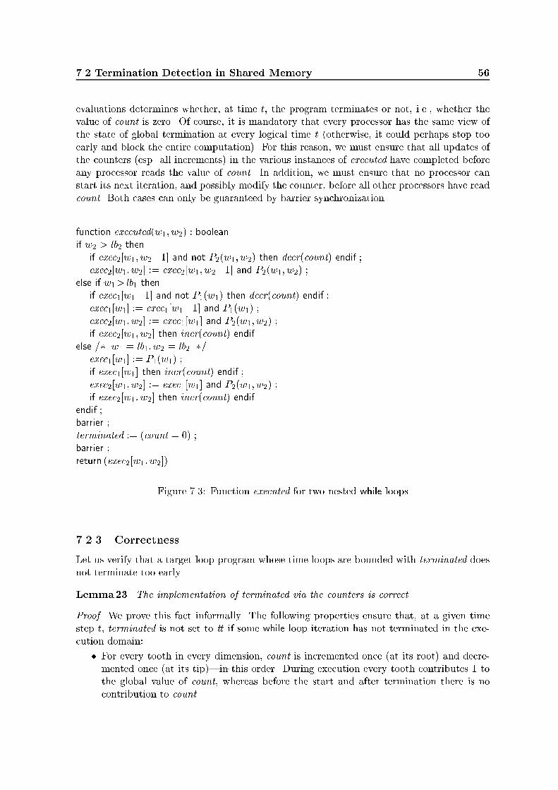
7.2 Termination Detection in Shared Memory 56evaluations determines whether, at time t, the program terminates or not, i.e., whether thevalue of count is zero. Of course, it is mandatory that every processor has the same view ofthe state of global termination at every logical time t (otherwise, it could perhaps stop tooearly and block the entire computation). For this reason, we must ensure that all updates ofthe counters (esp. all increments) in the various instances of executed have completed beforeany processor reads the value of count. In addition, we must ensure that no processor canstart its next iteration, and possibly modify the counter, before all other processors have readcount. Both cases can only be guaranteed by barrier synchronization.function executed(w1; w2) : booleanif w2 > lb2 thenif exec2[w1; w2�1] and not P2(w1; w2) then decr(count) endif ;exec2[w1; w2] := exec2[w1; w2�1] and P2(w1; w2) ;else if w1> lb1 thenif exec1[w1�1] and not P1(w1) then decr(count) endif ;exec1[w1] := exec1[w1�1] and P1(w1) ;exec2[w1; w2] := exec1[w1] and P2(w1; w2) ;if exec2[w1; w2] then incr(count) endifelse =� w1 = lb1; w2 = lb2 �=exec1[w1] := P1(w1) ;if exec1[w1] then incr(count) endif ;exec2[w1; w2] := exec1[w1] and P2(w1; w2) ;if exec2[w1; w2] then incr(count) endifendif ;barrier ;terminated := (count = 0) ;barrier ;return (exec2[w1; w2])Figure 7.3: Function executed for two nested while loops7.2.3 CorrectnessLet us verify that a target loop program whose time loops are bounded with terminated doesnot terminate too early.Lemma23. The implementation of terminated via the counters is correct.Proof. We prove this fact informally. The following properties ensure that, at a given timestep t, terminated is not set to tt if some while loop iteration has not terminated in the exe-cution domain:� For every tooth in every dimension, count is incremented once (at its root) and decre-mented once (at its tip)|in this order. During execution every tooth contributes 1 tothe global value of count, whereas before the start and after termination there is nocontribution to count.

7.2 Termination Detection in Shared Memory 57� Barrier synchronization ensures that all updates of count occur before the processorsread the value of count. Note that the order in which increments and decrements takeplace does not a�ect the �nal value.� If there is at least one processor evaluating some executedr(x1; � � � ; xd) (1� r�d) to ttat time t then the tooth � at level r and through the point (x1; � � � ; xr; lbr+1; � � � ; lbd)has started but not yet �nished execution. Thus, at this point in time, � is contributing1 to count.� Since � contributes 1 to count and since there cannot have been more decrements thanincrements, count must be strictly positive, thus preventing termination.7.2.4 OptimizationThe straight-forward implementation of the counter scheme in Figure 7.2 has an essentialdrawback: there is only one shared counter which can be updated by any iteration, i.e., thiscounter is a bottleneck.A better implementation would use multiple counters, each of which is only responsiblefor one r-dimensional subspace, thus avoiding many con icts. As soon as such a counterbecomes zero, the counter responsible for the next outer dimension is decremented. E.g., ifwe substitute r by d we get the scheme described before; if we substitute r by 1 we use onecounter per tooth.Note that in the latter case there may still be con icting accesses of the counters: if allteeth terminate at the same time, then the teeth started by some tooth � cause the counterof � to be decremented, which terminates � , and so on. All in all, we can have linearly manycon icting accesses of counters.Another optimization is necessary for bounding the size of array exec, for which we gaveno bound so far. J.-F. Collard [12] presents a way of determining a bound for arrays bycalculating the life time of the array elements and then introducing reassignments.7.2.5 The ExampleLet us now apply the counter scheme in the development of a synchronous and, thus, un-scannable target loop nest for our example program. For simplicity, Figures 7.4 to 7.6 showthe target loop nest and some auxiliary functions before partitioning.The target loop nest is presented in Figure 7.4, where (c ? e1 : e2) denotes a conditionalexpression whose value is e1 if condition c evaluates to tt and e2 otherwise. Note that, dueto the imperfect nesting, we must use a separate predicate terminated (and, thus, a separatecounter) for every source while dimension. In addition, we store the maximum value of allupper bounds of a loop at level l in max indexl. For while loops the value of this variableis not valid before the corresponding while loop terminates, i.e., max indexl contains a validvalue when terminatedl is tt .Let us now consider the guards in more detail. In principle there are rather simpleguards for non-loop statements and more complex guards for loop statements. We discussthe structure of the functions executed for the two cases by taking one example for each case;the guards for the other statements are very similar.For a guard of a non-loop statement, we choose arbitrarily predicate executed of statementS5 (Figure 7.5). The then branch of executed S5 checks for violations of the constraints of

7.2 Termination Detection in Shared Memory 58for t1 := 0 while t1 � (not terminated1 ? t1 : (not terminated2 ? t1 :max(4 �max index2+3+max index1;max index1))) doparfor p1 := min(t1�1; 0) to t1 doif executed S1(t1; p1) thenskipendifif executed S2(t1; p1) thenrt [t1�1; 0] := t1�1endifif executed S3(t1; p1) thennxt [t1�1] := 1endifif executed S4(t1; p1) thenskipendifif executed S5(t1; p1) thenif cond [p1; (t1�p1�5)=4] := (not Tag[p1; rt [p1; (t1�p1�5)=4]])endifif executed S6(t1; p1) and if cond [p1; (t1�p1�6)=4] thentag [p1; rt [p1; (t1�p1�6)=4]] := ttendifif executed S7(t1; p1) and if cond [p1; (t1�p1�6)=4] thenskipendifif executed S9(t1; p1) and if cond [p1; (t1�p1�8)=4] thennxt [p1] := nxt [p1]+nrsuc[rt [p1; (t1�p1�8)=4]]endiffor t2 := 0 to max for 0 0 0 doif executed S8(t1; p1; t2) and if cond [p1; (t1�p1�7)=4] thenrt [p1; t2+nxt [p1]] := suc[rt [p1; (t1�p1�7)=4]; t2]endifenddoenddoenddo Figure 7.4: The synchronous target programthe target index space, whereas the else branch checks for the remaining index points whetherthe current point belongs to the target execution space.As a representative of function executed of a loop statement we select executed S4 (Fig-ure 7.6). Function executed S4 �rst computes the new value of executed at the currentpoint. Then, it actualizes the counters and the variables max index storing the maximalloop bounds of a dimension. Between the synchronizations via the barrier, terminated iscomputed and the value of executed is returned. For implementation reasons, the value of

7.2 Termination Detection in Shared Memory 59function executed S5(t1; p1) : booleanif t1<5 or p1<0 or p1>t1�5 or (t1�p1�5)%4 thenreturn (ff )elsereturn (exec2[p1; (t1�p1�5)=4])endif Figure 7.5: executed S5function executed S4(t1; p1) : booleanif t1�4 and p1�0 and p1� t1�4 and (t1�p1�4)%4 = 0 thenif (t1�p1�4)=4 = 0 thenexec2[p1; (t1�p1�4)=4] := (rt [p1; (t1�p1�4)=4] 6= ?) and exec1[p1]elseexec2[p1; (t1�p1�4)=4] := (rt [p1; (t1�p1�4)=4] 6= ?) and exec2[p1; ((t1�p1�4)=4) � 1]endifif exec2[p1; (t1�p1�4)=4] thenskip =� would be incr(count3) if there were an inner while loop �=elseif ((t1�p1�4)=4 > 0 ? exec2[p1; (t1�p1�4)=4 � 1] : exec1[p1]) thendecr(count2)max index2 := max(max index2; (t1�p1�4)=4)endifelselocal index violation ag := ttendifbarrierif count2 = 0 thenterminated2 := ttendifbarrierif local index violation ag thenreturn (ff )elsereturn (exec2[p1; (t1�p1�4)=4])endif Figure 7.6: executed S4executed at points outside of the index space is not stored in the array exec but in a local ag local index violation ag . Note that the computed value of executed is stored in arrayexec, which allows us to access this value without re-calling function executed; this avoids theundesired re-computation of the side e�ects in executed.

7.3 Termination Detection with Distributed Memory 6013sig

sig32sig12 13sig

dimensions12 3

MP

Figure 7.7: A three-dimensional comb7.3 Termination Detection with Distributed MemoryIn this section we present a solution of the termination problem that requires only localcommunication.7.3.1 IdeaThe basic idea of our solution is as follows: if (carefully selected) teeth along dimension rof the execution space inform their (still executing) neighbors in dimensions 1; � � � ; r�1 oftheir termination, the maximal coordinates of every dimension of the execution space arecommunicated.If we ensure that no tooth terminates before it has been informed of the termination of itsneighbors, points that are involved in these communications are partially maximal until thepoint (x1;� � � ;xd) in S is reached whose coordinates are all maximal, i.e., have the property(8 x0 : x02X : (8 r : 1�r�d : x0r�xr)). When scanning this point, we can terminate alltarget loops.The propagation of the maxima, up to level r, proceeds by valueless signals. Signalsigrk(x1; � � � ; xr; lbr+1; � � � ; lbd) starts at point (x1;� � � ;xr;lbr+1;� � � ;lbd) at level r and is sent tothe neighboring tooth in direction k, where k is some outer level with respect to r, i.e., k<r.The main problem is how to establish whether a tooth can terminate immediately whenthe corresponding while condition is violated or whether it has to wait for some signal �rst.Example 10. Consider the three-dimensional comb of Figure 7.7.Our scheme is more easily understood in the synchronous model.In the �gure, the teeth of X are represented by solid lines. Some teeth are extended bydotted lines, indicating that they are waiting for at least one signal. Points (of S) on dotted

7.3 Termination Detection with Distributed Memory 61lines do not execute the loop body, they only wait for signals. Signals are represented bydashed arrows.Our aim is to identify the point M whose coordinates are maximal in every dimension.The �rst coordinate of M is quite easy to determine: it is the value at which the outermostloop terminates.The second coordinate of M is the maximum of the lengths of all teeth pointing up (inthe �gure). To determine it, every vertical tooth tells its right neighbor the maximum of itsown height and the maximal height left of it. This is the meaning of sig21. If a vertical toothis ready to terminate but did not yet receive sig21 from its left neighbor, it must wait (exceptfor the leftmost tooth) until this signal is received. (In the �gure, the tooth at the right mustwait.) Then it itself sends sig21 on to its right neighbor and terminates. The following formalproperty holds for all teeth in dimension 2:sig21(x1; x2; lb3)) (8 x01; x02 : (x01; x02; lb03)2X ^ x01�x1 : x02�x2)The determination of the maximal depth of teeth in each vertical plane (x1 constant)proceeds analogously. Signals sig32 are sent from every (perhaps extended, since waiting)tooth � along dimension 3 to its upper neighbor of that plane, indicating that the currentdepth (the length of �) is maximal for all teeth in dimension 3 to the left and including � , for�xed x1. Formally:sig32(x1; x2; x3)) (8 x02; x03 : (x1; x02; x03)2X ^ x02�x2 : x03�x3)To combine the maxima of all vertical planes, the maximal point of each plane sends asignal sig31 to its right neighbor. Again, it is important that this right neighbor must notterminate before the signal is received. Which teeth must wait? The maximal depth in everyvertical plane is reached at the end of the (perhaps extended) vertical tooth that forms thebase of this plane. This height was propagated to the right neighbor by sig21. At that height,the maximal depth will also be propagated. Therefore, the tooth, rooted at that point (e.g.,P in the �gure) which received sig21 and which points into dimension 3 (the thick tooth in the�gure), must wait until sig31 is received. Again, formally:sig31(x1; x2; x3)) (8 x01; x02; x03 : (x01; x02; x03)2X ^ x01�x1 : x02�x2 ^ x03�x3)The formal properties implied by the signals form a pattern that we call the partialmaximality (of a point). M is partially maximal with respect to all dimensions and is,therefore, the maximal point.7.3.2 FormalizationIn the following, we de�ne partial maximality recursively for an arbitrary number of dimen-sions. Then we construct a mechanism that sends signals from partially maximal points tothe appropriate destinations.To include the host of the processor array, we introduce a little hack. We imagine onemore dimension, 0, which has extent 2. The polyhedron is located at position 0, and the hostat position 1. Then we introduce signals that travel from position 0 to position 1. They aremeant to communicate the termination of the target loops to the host.

7.3 Termination Detection with Distributed Memory 62De�nition 24 (Partial maximality mrk). mrk(x1; � � � ; xr; lbr+1; � � � ; lbd) i� for �xed indicesat levels 1 to k� 1 and for points (x01; � � � ; x0r) below (x01; � � � ; x0r; lb0r+1; � � � ; lb0d) at level k(x0k� xk), point (x1;� � � ;xr;lbr+1;� � � ;lbd) is maximal in all dimensions k+1; � � � ; r. Formally:(8 r : 0<r�d : (8 (x1; � � � ; xr) : (x1; � � � ; xr; lbr+1; � � � ; lbd)2 bX :(8 k : 0�k<r : mrk(x1; � � � ; xr; lbr+1; � � � ; lbd) =(8 x0k; � � � ; x0r : (x1; � � � ; xk�1; x0k; � � � ; x0r; lb0r+1; � � � ; lb0d)2 bX ^ x0k�xk :x0k+1�xk+1; � � � ; x0r�xr))))If mrk(x1; � � � ; xr; lbr+1; � � � ; lbd), we call point (x1;� � � ;xr;lbr+1;� � � ;lbd) partially maximal withrespect to dimensions k+1 to r.Note that, for k=0, the right-hand side of De�nition 24 simpli�es to:(8 x01; � � � ; x0r : (x01; � � � ; x0r; lb0r+1; � � � ; lb0d)2 bX : x01�x1 ^ � � � ^ x0r�xr)For our communication scheme of m by signals, we need an additional predicate, wrk(x1;� � � ; xr; lbr+1; � � � ; lbd), which indicates that the tooth that is rooted at (x1;� � � ;xr�1;lbr; � � � ; lbd)and extends along dimension r must wait until signal sigrk arrives at some point (x1;� � � ;xr�1;x0r;lbr+1; � � � ; lbd) with x0r � xr. These additional points at which a tooth waits but executesnothing make the di�erence between S and X . The lemmata that follow are valid for allpoints in S.De�nition 25 (sig and w).(8 (x1; � � � ; xd) : (x1; � � � ; xd)2I : (8 k; r : 0�k<r�d : sigrk(x1; � � � ; xr; lbr+1; � � � ; lbd) =:executedr(x1; � � � ; xr; lbr+1; � � � ; lbd)^(8 s : 1�s<r : :wrs(x1; � � � ; xr; lbr+1; � � � ; lbd) _ sigrs(x1; � � � ; xs�1; � � � ; xr; lbr+1; � � � ; lbd))^(r>k+1) sigr�1k (x1; � � � ; xr�1; lbr; � � � ; lbd)) ))For all other points sig is initialized with ff :(8 (x1; � � � ; xd) : (x1; � � � ; xd)2Zd�I : (8 k; r : 0�k<r�d :sigrk(x1; � � � ; xr; lbr+1; � � � ; lbd) = ff ))(8 (x1; � � � ; xd) : (x1; � � � ; xd)2I : (8 k; r : 0�k<r�d : wrk(x1; � � � ; xr; lbr+1; � � � ; lbd) =if k=0 ! ff (1)[] r=k+1 ^ k>0 ^ xk+1= lbk+1 ! xk 6= lbk (2)[] r>k+1 ^ k>0 ^ xk+1= lbk+1 ! sigr�1k (x1; � � � ; xk�1; � � � ; xr�1; lbr; � � � ; lbd) (3)[] r�k+1 ^ k>0 ^ xr> lbr ! wrk(x1; � � � ; xr�1; xr�1; lbr+1; � � � ; lbd) ^ (4):sigrk(x1; � � � ; xk�1; � � � ; xr�1; xr�1; lbr+1; � � � ; lbd)� ))These equations can be explained as follows.sig states that any point of a tooth that need not be executed and that does not have towait for any signal sends signal sigrk if either the tooth and the signal lie in a two-dimensionalplane (recursion base) or the root (x1;� � � ;xr�1;lbr; � � � ; lbd) of the tooth has already sent thesignal into the same direction (recursion).wrk(x1; � � � ; xr; lbr+1; � � � ; lbd) states whether the point (x1; � � � ; xr; lbr+1; � � � ; lbd) at level rhas to wait for some signal from direction k:

7.3 Termination Detection with Distributed Memory 63(1) No point has to wait for signals from the host.(2) In every two-dimensional subspace (dimensions k and r = k+1), every tooth, i.e., atleast the �rst point of it (with xk+1 = lbk+1), has to wait for a signal from the toothimmediately preceding it|if any, i.e., if xk 6= lbk.(3) In every at least three-dimensional subspace (dimensions k to r > k+1), every toothparallel to dimension r, i.e., at least the �rst point of it, has to wait for some signalfrom direction k i� its root at level r�1 has received a signal from the same direction k.(4) Any point of a tooth that is not the �rst point has to wait for a signal i� its predecessoron the tooth had to wait and did not receive the signal it was waiting for.7.3.3 Signals and their Signi�cance for Local MaximalityThe main result of this subsection is that signals sig correctly propagate property m of localmaximality. We state this in two separate lemmata.Lemma26 (Local maximum). A point of some tooth along dimension r that need not beexecuted with respect to r and need not wait for a signal is maximal with respect to dimensionr. Formally:(8 x1; � � � ; xr : (x1; � � � ; xr; lbr+1; � � � ; lbd)2S : :executedr(x1; � � � ; xr; lbr+1; � � � ; lbd) ^(8 s : 1�s<r : (:wrs(x1; � � � ; xr; lbr+1; � � � ; lbd) _sigrs(x1; � � � ; xs�1; � � � ; xr; lbr+1; � � � ; lbd))))(8 x0r : (x1; � � � ; xr�1; x0r; lbr+1; � � � ; lbd)2S : x0r�xr))Proof. We prove the inverse implication: (H ) C), (:C ) :H).:(8 x0r : (x1; � � � ; xr�1; x0r; lbr+1; � � � ; lbd)2S : x0r�xr), f predicate calculus g(9 x0r : (x1; � � � ; xr�1; x0r; lbr+1; � � � ; lbd)2S : x0r>xr)) f if point (x1; � � � ; xr�1; x0r; lbr+1; � � � ; lbd) is scanned, it must be exe-cuting or waiting g(9 x0r : (x1; � � � ; xr�1; x0r; lbr+1; � � � ; lbd)2S : executedr(x1; � � � ; xr�1; x0r; lbr+1; � � � ; lbd) _(9 s : 1�s<r : (wrs(x1; � � � ; xr�1; x0r; lbr+1; � � � ; lbd)^:sigrs(x1; � � � ; xs�1; � � � ; x0r; lbr+1; � � � ; lbd)))) f predicate calculus g:(8 (x1; � � � ; xr) : (x1; � � � ; xr; lbr+1; � � � ; lbd)2S : :executedr(x1; � � � ; xr; lbr+1; � � � ; lbd) ^(8 s : 1�s<r : :wrs(x1; � � � ; xr; lbr+1; � � � ; lbd) _ sigrs(x1; � � � ; xs�1; � � � ; xr; lbr+1; � � � ; lbd)))In the following lemma, SUBrk(x1; � � � ; xk�1) is the subspace of S in dimensions k to r(1�k<r�d) and at �xed coordinates (x1;� � � ;xk�1).Lemma27 (sig implements m).(8 k; r : 0�k<r�d : (8 (x1; � � � ; xr) : (x1; � � � ; xr; lbr+1; � � � ; lbd)2S :sigrk(x1; � � � ; xr; lbr+1; � � � ; lbd)) mrk(x1; � � � ; xr; lbr+1; � � � ; lbd)))

7.3 Termination Detection with Distributed Memory 64Proof. By induction on the dimension of SUBrk(x1; � � � ; xk�1).� Induction base (r = k+1):For sigk+1k (x1; � � � ; xk�1; lbk; � � � ; lbd) ) mk+1k (x1; � � � ; xk�1; lbk; � � � ; lbd) we must distin-guish two cases, since x0 does not exist.{ First case: k = 0sig10(x1; lb2; � � � ; lbd), f de�nition of sig with k = 0, r = 1 g:executed1(x1; lb2; � � � ; lbd)) f Lemma 26 with k = 0, r = 1 g(8 x01 : (x01; lb2; � � � ; lbd)2S : x01�x1), f de�nition of m10 gm10(x1; lb2; � � � ; lbd){ Second case: k > 0We prove sigk+1k (x1; � � � ; xk�1; lbk; � � � ; lbd) ) mk+1k (x1; � � � ; xk�1; lbk; � � � ; lbd) by in-duction on xk.� Induction base (xk = lbk):sigk+1k (x1; � � � ; xk�1; lbk; � � � ; lbd), f de�nition of sig with xk = lbk and simpli�cation for r = k+1 g:executedk+1(x1; � � � ; xk�1; lbk; � � � ; lbd) ^ (8 s : 1�s<k+1 ::wk+1s (x1; � � � ; xk�1; lbk; � � � ; lbd)_sigk+1s (x1; � � � ; xs�1; � � � ; xk+1; lbk+2; � � � ; lbd))) f Lemma 26 g(8 x0k+1 : (x1; � � � ; xk; x0k+1; lbk+2; � � � ; lbd)2S : x0k+1�xk+1), f lbk is the smallest xk; introduction of a new dummy with emptyrange g(8 x0k; x0k+1 : (x1; � � � ; xk�1; x0k; x0k+1; lbk+2; � � � ; lbd)2S ^ x0k�xk :x0k+1�xk+1), f de�nition of m gmk+1k (x1; � � � ; xk�1; lbk; � � � ; lbd)� Induction step (xk�1! xk, where xk> lbk):sigk+1k (x1; � � � ; xk�1; lbk; � � � ; lbd), f de�nition of sig with xk > lbk and simpli�cation for r = k+1 g:executedk+1(x1; � � � ; xk�1; lbk; � � � ; lbd) ^ (8 s : 1�s<k+1 :(:wk+1s (x1; � � � ; xk�1; lbk; � � � ; lbd)_sigk+1s (x1; � � � ; xs�1; � � � ; xk+1; lbk+2; � � � ; lbd))), f duplicate of:wk+1k _ sigk+1k (x1; � � � ; xk�1; xk�1; xk+1; lbk+2; � � � ; lbd) g

7.3 Termination Detection with Distributed Memory 65:executedk+1(x1; � � � ; xk�1; lbk; � � � ; lbd) ^ (8 s : 1�s<k+1 :(:wk+1s (x1; � � � ; xk�1; lbk; � � � ; lbd)_sigk+1s (x1; � � � ; xs�1; � � � ; xk+1; lbk+2; � � � ; lbd))) ^:wk+1k (x1; � � � ; xk�1; lbk; � � � ; lbd)_sigk+1k (x1; � � � ; xk�1; xk�1; xk+1; lbk+2; � � � ; lbd)) f Lemma 26 g(8 x0k+1 : (x1; � � � ; xk; x0k+1; lbk+2; � � � ; lbd)2S : x0k+1�xk+1) ^:wk+1k (x1; � � � ; xk�1; lbk; � � � ; lbd)_sigk+1k (x1; � � � ; xk�1; xk�1; xk+1; lbk+2; � � � ; lbd)) f by structural induction on the de�nition of w g(8 x0k+1 : (x1; � � � ; xk; x0k+1; lbk+2; � � � ; lbd)2S : x0k+1�xk+1) ^ (xk = lbk _(9[xk+1 : [xk+1�xk+1 : sigk+1k (x1; � � � ; xk�1;[xk+1; lbk+2; � � � ; lbd))), f xk 6= lbk (induction step) g(8 x0k+1 : (x1; � � � ; xk; x0k+1; lbk+2; � � � ; lbd)2S : x0k+1�xk+1) ^(9[xk+1 : [xk+1�xk+1 : sigk+1k (x1; � � � ; xk�1;[xk+1; lbk+2; � � � ; lbd))) f induction hypothesis for sigk+1k (x1; � � � ; xk�1;[xk+1; lbk+2; � � � ; lbd) g(8 x0k+1 : (x1; � � � ; xk; x0k+1; lbk+2; � � � ; lbd)2S : x0k+1�xk+1) ^(9[xk+1 : [xk+1�xk+1 : mk+1k (x1; � � � ; xk�1;[xk+1; lbk+2; � � � ; lbd)), f[xk+1�xk+1; de�nition of m) g(8 x0k+1 : (x1; � � � ; xk; x0k+1; lbk+2; � � � ; lbd)2S : x0k+1�xk+1) ^mk+1k (x1; � � � ; xk�1; xk+1; lbk+2; � � � ; lbd), f de�nition of m g(8 x0k+1 : (x1; � � � ; xk; x0k+1; lbk+2; � � � ; lbd)2S : x0k+1�xk+1) ^ (8 x0k; x0k+1 :(x1; � � � ; xk�1; x0k; x0k+1; lbk+2; � � � ; lbd)2S ^ x0k�xk�1 : x0k+1�xk+1), f combination of two quanti�cation ranges g(8x0k; x0k+1 : (x1; � � � ; xk�1; x0k; x0k+1; lbk+2; � � � ; lbd)2S ^x0k�xk : x0k+1�xk+1), f de�nition of m gmk+1k (x1; � � � ; xk�1; lbk; � � � ; lbd)� Induction step (k ! k�1, where r�k > 1):sigrk�1(x1; � � � ; xr; lbr+1; � � � ; lbd), f de�nition of sig with r > k+1 g:executedr(x1; � � � ; xr; lbr+1; � � � ; lbd) ^ (8 s : 1�s<r ::rs(x1; � � � ; xr; lbr+1; � � � ; lbd) _ sigrs(x1; � � � ; xs�1; � � � ; xr; lbr+1; � � � ; lbd)) ^sigr�1k�1(x1; � � � ; xr�1; lbr; � � � ; lbd)) f Lemma 26 g(8 x0r : (x1; � � � ; xr�1; x0r; lbr+1; � � � ; lbd)2S : x0r�xr) ^sigr�1k�1(x1; � � � ; xr�1; lbr; � � � ; lbd)) f induction hypothesis for sigr�1k�1 g(8 x0r : (x1; � � � ; xr�1; x0r; lbr+1; � � � ; lbd)2S : x0r�xr) ^mr�1k�1(x1; � � � ; xr�1; lbr; � � � ; lbd), f de�nition of m g

7.3 Termination Detection with Distributed Memory 66(8 x0r : (x1; � � � ; xr�1; x0r; lbr+1; � � � ; lbd)2S : x0r�xr) ^(8 x0k�1; � � � ; x0r�1 : (x1; � � � ; xk�2; x0k�1; � � � ; x0r�1; lbr; � � � ; lbd)2S ^ x0k�1�xk�1 :x0k�xk ^ � � � ^ x0r�1�xr�1)) f combination of two quanti�cation ranges g(8 x0k; � � � ; x0r : (x1; � � � ; xk�2; x0k�1; � � � ; x0r; lbr+1; � � � ; lbd)2S ^ x0k�1�xk�1 :x0k�xk ^ � � � ^ x0r�xr), f de�nition of m gmrk�1(x1; � � � ; xr; lbr+1; � � � ; lbd)Our aim has been to identify the point of S with maximal coordinates in all dimensions.The scanning of this point indicates the termination of the entire target loop nest. We haveconstructed a signaling scheme in which this point sends signal sigd0 to the host.Remark 28 (Optimization).� A tooth in direction r must send at least one signal, into direction r�1.� One simple optimization can be made immediately: signals need not be sent to pointsx along a tooth that has terminated, i.e., points that neither are active nor wait for asignal. Thus, sigrk(x1; � � � ; xr; lbr+1; � � � ; lbd) implies that, for any k0 with k0<k, sigrk0(x1;� � � ; xr; lbr+1; � � � ; lbd) need not be sent. In Example 10 we have already omitted thesesignals, but they are of course part of De�nition 25. Thus every terminating tooth hasto send at most one signal.� In summary, every tooth must send exactly one signal when it terminates.7.3.4 Target Code Generation for Distributed Memory MachinesIn the remainder of this section we derive code for the target program. In a straight-forwardimplementation we could augment the source program by an implementation of the predicatesand the signals, developed in the previous sections, and apply the space-time mapping to thisaugmented source program.However, since the transformation of the signaling scheme is problem-independent wedecided to derive a skeleton for the transformed signaling scheme which can be �lled withthe problem-speci�c body statements and transformations. This strategy also unburdens thetarget generator of a parallelizing compiler signi�cantly, which accelerates the target codegeneration.Thus, we present an augmentation of the target loop body such that the irregular shapeof the transformed execution space is dealt with properly. Our augmentation implements thesignaling scheme presented above. We prove that, while the target loops enumerate TS, theaugmented body reduces the execution of the loop nest to precisely the points of TX .7.3.4.1 General TechniqueFirst we present the target code which is abstract in the sense that it is neither optimized formemory usage (it is single-assignment!) nor adapted to the execution model (synchronous orasynchronous) of the target machine. These adaptations are given in Section 7.3.4.3.

7.3 Termination Detection with Distributed Memory 67The target code must specify communications (send and receive primitives) explicitly.We use three primitives that are executable on the Parix1 operating system [45], one fortransmitting and two for receiving. The reception mode depends on the type of messagetransmitted.Our signaling scheme contains two types of messages.� One type is responsible for the propagation of information along one tooth. An exampleis the value of the predicate active. The receipt of a message of this type is necessaryfor the execution of the loop body at the respective point.� The other type of messages is for signals sig. These signals must be \probed" [42], sinceexecution of a loop iteration may proceed without their receipt.Let us brie y describe the three primitives:� asend(dir; list of vals) is a Parix command that transmits a list of values into a speci-�ed direction in (d�1)-dimensional space. Communication is asynchronous to preventdeadlocks.� receive(dir; list of vals) is a Parix command that performs a blocking receive of a listof values from a speci�ed direction.� creceive(dir; list of vals) is a command de�ned by us that performs a non-blocking receiveof a list of values from a speci�ed direction. Martin [42] de�nes the value of a probeY on some communication action Y as a boolean value that indicates whether thecorresponding communication action is pending. In our context, Y is a receive commandfrom some direction and, thus, Y holds i� the corresponding asend command did alreadytake place. With this construct, we de�ne creceive(dir; list of vals) as follows:if receive(dir; list of vals) then receive(dir, list of vals) endif.Note: receive(dir; list of vals) corresponds roughly to the Parix commandSelect(ReceiveOption(dir)) [45].We are now able to present the single-assignment target program. For readability weonly describe the case of a perfect loop nest; the technical modi�cations for the general casecan be found in [33]. Also for simplicity, we implement termination by the Parix commandAbortServer which is executed only by the iteration that is maximal for all dimensions (i.e.,partially maximal with respect to dimensions 1 to d, as de�ned in De�nition 24). Thus, thewhile loops in the target program need no upper bound.The skeleton of the target loop nest is displayed in Figure 7.8 and re�ned in the subsequentFigures 7.9 and 7.10. This code is for asynchronous parallel execution on machines withdistributed memory. The necessary changes for synchronous execution and/or shared memoryare discussed in Section 7.3.4.3.Note that the loops in the �gure represent the worst case of a nest with only while loops,which are therefore sequential (remember that there is no parallel while loop). However, thisis not typical, since the parallel loops (which hopefully do exist) can be written as (parallel)for loops (Remark 21 on page 49). Thus, some of the while loops in the scheme are replacedby parfor loops.1ParixTM is an operating system for parallel computers with distributed memory by the Parsytec com-pany based on the SPMD programming model [46].

7.3 Termination Detection with Distributed Memory 68k1(lb1) := 0prg-active1(lb1) := ttfor y1 := lb1 while tt do... for yd := lbd while tt dobpre1 (x1)...bpred (x1; � � � ; xd)if prg-actived(x1; � � � ; xd) and conditiond(x1; � � � ; xd) thenb(x1; � � � ; xd)endifbpost1 (x1)...bpostd (x1; � � � ; xd)enddo...enddo Figure 7.8: The target loop nestThe augmentation of the loop body for every level r, i.e., br(x1; � � � ; xr), consists of twoparts:� The pre�x bprer (x1; � � � ; xr), executed before the transformed source loop body, is dis-played in Figure 7.9. It receives all necessary data and calculates the output values ofall variables that are introduced by our signaling scheme.� The post�x bpostr (x1; � � � ; xr), executed after the source loop (at least for asynchronousexecution, see Remark 29), is displayed in Figure 7.10. It is responsible for sending allnecessary information.Let us now discuss the code in detail:Variables:� chanSk represents the channel for the signals that travel along dimension k. chanDrrepresents the channel for the data, i.e., prg-activer, kr, and prg-wrk, 1�k<r, thatare propagated along every tooth.� kr is the direction in which the tooth must send a signal before it terminates. Itcorresponds to the lower index k of sigrk(x1; � � � ; xr). The optimization outlined inRemark 28 ensures that there is a unique k for each tooth.� sigvalr corresponds to sigrk in De�nition 25 (more precisely, it guarantees the �rsttwo conjuncts of De�nition 25, cf. Lemma 35).

7.3 Termination Detection with Distributed Memory 69(8 r : 1�r�d : bprer (x1; � � � ; xr) :if xr+1= lbr+1 and � � � and xd= lbd thenA : 8>>>><>>>>: /* receive signals */creceive(chanS1 ; [rcvedr1(x1; � � � ; xr)])...creceive(chanSr�1; [rcvedrr�1(x1; � � � ; xr)])B : 8><>: /* receive data */receive(chanDr ; [prg-activer(x1; � � � ; xr); kr(x1; � � � ; xr);prg-wr1(x1; � � � ; xr); � � � ; prg-wrr�1(x1; � � � ; xr)])/* calculate output values for all signals */C : 8><>: prg-wr1(x1; � � � ; xr+1) := prg-wr1(x1; � � � ; xr) and not rcvedr1...prg-wrr�1(x1; � � � ; xr+1) := prg-wrr�1(x1; � � � ; xr) and not rcvedrr�1D : 8>>>><>>>>: prg-wr+11 (x1; � � � ; xr; lbr+1) := rcvedr1(x1; � � � ; xr)...prg-wr+1r�1(x1; � � � ; xr; lbr+1) := rcvedrr�1(x1; � � � ; xr)prg-wr+1r (x1; � � � ; xr; lbr+1) := (xr 6= lbr) 9>>>>=>>>>; only for r<dE : kr(x1; � � � ; xr + 1) := kr(x1; � � � ; xr)if prg-activer(x1; � � � ; xr) and conditionr(x1; � � � ; xr) thensigvalr(x1; � � � ; xr) := ffprg-activer(x1; � � � ; xr+1) := ttprg-activer+1(x1; � � � ; xr; lbr+1) := ttF : kr+1(x1; � � � ; xr; lbr+1) := r ) only for r<delseG : prg-wr(x1; � � � ; xr) := prg-wr1(x1; � � � ; xr+1) or � � � or prg-wrr�1(x1; � � � ; xr+1)sigvalr(x1; � � � ; xr) := not prg-wr(x1; � � � ; xr)prg-activer(x1; � � � ; xr+1) := ffprg-activer+1(x1; � � � ; xr; lbr+1) := ffH : 8>>>>><>>>>>: if sigvalr(x1; � � � ; xr) thenkr+1(x1; � � � ; xr; lbr+1) := kr(x1; � � � ; xr)elsekr+1(x1; � � � ; xr; lbr+1) := rendif

9>>>>>>>=>>>>>>>; only for r<dendifendif) Figure 7.9: The pre�x of the transformed loop body

7.3 Termination Detection with Distributed Memory 70(8 r : 1�r�d : bpostr (x1; � � � ; xr) :if xr+1= lbr+1 and � � � and xd= lbd thenI : 8><>: if kr(x1; � � � ; xr) = 0 and sigvalr(x1; � � � ; xr) thenAbort Server()endif 9>=>; only for r=dJ : 8><>: /* send data */asend(chanDr ; [prg-activer(x1; � � � ; xr+1); kr(x1; � � � ; xr+1);prg-wr1(x1; � � � ; xr+1); � � � ; prg-wrr�1(x1; � � � ; xr+1)])K : 8>>><>>>: /* send signals */if kr(x1; � � � ; xr) 6= 0 and sigvalr(x1; � � � ; xr) thenasend(chanSkr ; [tt ])endifendif) Figure 7.10: The post�x of the transformed loop body� prg-activer(x) is the counterpart of the predicate active in the source loop nest,i.e., for every point x of I, the value of prg-activer(x) at the end of the programis equal to the value of activer(x). We say prg-active implements predicate activeand prove this fact in Lemma 33. The value of prg-active(x) is unde�ned if T x isnot scanned by the target loop nest.� Analogously, prg-wrk is the counterpart of wrk in De�nition 25.Execution:� The outermost if clause prevents the body from receiving, calculating and sendingsignals and messages that are not speci�ed by our signaling scheme of De�nition 25,i.e., signals at depth r0>r.� Part A probes signals that are expected and receives those that are actually beingsent. Thus, rcvedrk(x1; � � � ; xr) is equal to sigrk(x1; � � � ; xk�1; � � � ; xr).� Part B propagates all necessary information along the tooth in direction r.� Part C implements alternative (4) of De�nition 25.� All but the last line of part D implements alternative (3); the last line implementsalternative (2).� Line E copies the value of k for the next iteration.� The if clause after line E tests whether the current iteration must be executedwith respect to level r (De�nition 16). The value of prg-activer, sigvalr and, if theyexist, prg-activer+1 and kr+1 depend on the outcome of the test.� sigrk has three conjuncts (De�nition 25). The �rst corresponds to the then or theelse branch of said if clause, the second to the calculation at line G. The thirdconjunct is satis�ed by an appropriate setting of kr in parts F and H.

7.3 Termination Detection with Distributed Memory 71� prg-active implements active (De�nition 15), as proved in Lemma 33.� Part I applies only for r= d. It tests for sigd0 (i.e., sigvald and kd=0) and, if so,terminates the entire program (compare Lemma 27 and De�nition 24).� Part J sends the data that are received by Part B on to the next point of thetooth.� Part K sends sigrk, if it has to be sent, i.e., if sigval holds. (At present, we ignoresignals in direction 0, but one could probably use this information to developsmarter loop bounds.)Remark 29. In the synchronous model, we obtain the same semantics if the post�xes aremade pre�xes instead. This is an optimization if each processor has a co-processor for thetransmission of messages so that computation and message handling can proceed in parallel, asis the case for the transputer [34]. For asynchronous machines, there is no similar optimizationsince only the receipt of messages can guarantee that the sender has updated all transformedsource variables.7.3.4.2 Correctness ProofIn this section, we prove that the target program executes the transformed source loop bodyfor all points whose inverse image is in the execution space.For the following proofs, we need a formal de�nition of TS, the set of target points thatare scanned by the target program. Note that the target while loops have no upper bounds:they enumerate an in�nite set. Our way of terminating the target program is by calling theParix command AbortServer at some point. This call terminates the whole program. Thus,points of TI are scanned until the AbortServer command is issued at some point. This leadsto the following de�nition:De�nition 30 (prg-scanned, S and TS). The image of a point x2I is scanned by the targetprogram if all points with a schedule not larger than t(x) do not call the AbortServer command,where the call of AbortServer is guarded by the condition kr(x0)=0^ sigvalr(x0) (Figure 7.10,Part I). Formally: (8 x : x2I : prg-scanned(x) =(8 x0 : x02I ^ t(x0)� t(x) : :(kr(x0)=0 ^ sigvald(x0))))S = fx2I : prg-scanned(x)gTS = fT x2TI : prg-scanned(x)gTo be able to reason about target points whose transformed loop body is executed, we needalso a formal de�nition of those points. The target program executes the transformed loopbody i� the point is scanned and prg-actived(x1; � � � ; xd)^ conditiond(x1; � � � ; xd) (Figure 7.8).Thus, we de�ne a predicate prg-exec accordingly and prove (Theorem 41) that the transformedloop body is executed exactly for those points that belong to the execution space, i.e., thatprg-exec(y) is equal to executed(T �1y) for all points y2TI.De�nition 31 (prg-exec).(8 x : x2I : prg-exec(x) = prg-scanned(x) ^ prg-actived(x) ^ conditiond(x))

7.3 Termination Detection with Distributed Memory 72This de�nition makes sense only if prg-active is never reassigned. The following auxiliarylemma to that e�ect is proved informally.Lemma32. Every variable prg-activer(x1; � � � ; xr), 1 � r � d and (x1; � � � ; xr; lbr+1; � � � ; lbd)2I, is assigned at most once during the execution of the transformed code.Proof. Every prg-activer(x1; � � � ; xr) occurs exactly once as left hand side of an assignment.Three disjoint cases cover every point (x1;� � � ;xr;lbr+1;� � � ;lbd) of I:1. if (r=1 ^ xr= lbr), it is assigned by the initialization statement prg-active1(lb1) := tt ;2. if (1<r<d^xr= lbr), it is assigned by prg-activer+1(x1; � � � ; xr; lbr+1) := tt in the thenbranch of bprer�1(x1; � � � ; xr�1);3. if xr> lbr, it is assigned either by prg-activer(x1; � � � ; xr+1) := tt or by prg-activer(x1;� � � ; xr+1) := ff in the then branch or the else branch of bprer (x1; � � � ; xr), respectively.Since no point is scanned more than once, we conclude that prg-activer(x1; � � � ; xr) is assignedat most once for any (x1;� � � ;xr).In the succeeding lemmata we prove properties of the target program. Thus, we need torefer to values of program variables. In our single-assignment setting, we are only interestedin the values at the end of the execution of the target program. This allows us to compute thevalues of some variables from the values of other variables by straight-forward code inspection.First, we prove that predicate active is implemented correctly.Lemma33. prg-activer implements activer for all points of I where the value of prg-activeris de�ned, i.e., whose image is scanned by the target program. Formally:(8 r; (x1; � � � ; xd) : 1�r�d ^ T (x1; � � � ; xd)2TS :prg-activer(x1; � � � ; xr) = activer(x1; � � � ; xr; lbr+1; � � � ; lbd))Proof. Induction over the nesting depth r, and then induction over the index range of the rloop.� Induction base (r = 1):{ Induction base (x1 = lb1):x1 = lb1) f de�nition of prg-active (Figure 7.8) and active gprg-active1(x1) = tt = active1(x1; lb2; � � � ; lbd){ Induction step (x1�1! x1, where x1> lb1):prg-active1(x1), f de�nition of prg-active1(x1) in the if clause of b1(x1�1): gprg-active1(x1�1) ^ condition1(x1�1), f induction hypothesis for x1�1 gactive1(x1�1; lb2; � � � ; lbd) ^ condition1(x1�1), f de�nition of activer for r = 1 and x1> lb1 gactive1(x1; lb2; � � � ; lbd)

7.3 Termination Detection with Distributed Memory 73� Induction step (r�1! r, where r>1):{ Induction base (xr= lbr):prg-activer(x1; � � � ; xr�1; lbr), f de�nition of prg-active1(x1) in the if clause of br�1(x1; � � � ; xr�1): gprg-activer�1(x1; � � � ; xr�1) ^ conditionr�1(x1; � � � ; xr�1), f induction hypothesis for r � 1 gactiver�1(x1; � � � ; xr�1; lbr; � � � ; lbd) ^ conditionr�1(x1; � � � ; xr�1), f de�nition of activer for r>1 and xr= lbr gactiver(x1; � � � ; xr; lbr+1; � � � ; lbd){ Induction step ((x1; � � � ; xr�1)! (x1; � � � ; xr), where xr> lbr):analogously to x1�1! x1.Next, we prove that predicate sig (De�nition 25) is also implemented correctly. We proceedin several steps:1. The following de�nition, De�nition 34, gives the predicate that corresponds to sig inthe target program a name: prg-sig.2. Two auxiliary lemmata lead up to Corollary 37, which expresses prg-sig analogously tothe de�nition of sig.3. This correspondence is helpful for the proof of Lemma 38, which states that prg-sigimplies sig.According to Figure 7.10, Part K, a signal is sent if (kr(x) 6= 0)^sigvalr(x). The directionof this signal is kr(x). This leads to the following de�nition:De�nition 34 (prg-sigrk). In the target program, a signal is sent into direction k i� the di-rection given by kr(x) equals k and sigvalr(x) holds. Formally:(8 r : 1�r<d : (8 (x1; � � � ; xr) : T (x1; � � � ; xr; lbr+1; � � � ; lbd)2TS : (8 k : 0�k<r :prg-sigrk(x1; � � � ; xr) = (kr(x1; � � � ; xr) = k) ^ sigvalr(x1; � � � ; xr))))where kr(x) is de�ned in parts E, F and H the target program.Lemma35. If a point T (x1; � � � ; xd) is scanned by the target program, the value of sigvalr(second conjunct of De�nition 34) is analogous to the �rst two conjuncts of the de�nition ofsig (De�nition 25). Formally:(8 (x1; � � � ; xd) : T (x1; � � � ; xd)2TS : (8 r : 0<r�d : sigvalr(x1; � � � ; xr) =:executedr(x1; � � � ; xr; lbr+1; � � � ; lbd) ^(8 s : 1�s<r : :prg-wrs(x1; � � � ; xr) _ prg-sigrs(x1; � � � ; xs�1; � � � ; xr)) ))Proof. Following the program, we distinguish two cases.� Case 1 (prg-activer(x1; � � � ; xr) ^ conditionr(x1; � � � ; xr)):In this case, executedr(x1; � � � ; xr; lbr+1; � � � ; lbd) holds:

7.3 Termination Detection with Distributed Memory 74executedr(x1; � � � ; xr; lbr+1; � � � ; lbd), f De�nition 16 gactiver(x1; � � � ; xr; lbr+1; � � � ; lbd) ^ conditionr(x1; � � � ; xr), f Lemma 33 gprg-activer(x1; � � � ; xr) ^ conditionr(x1; � � � ; xr), f condition of the �rst case gttThus, :executedr(x1; � � � ; xr; lbr+1; � � � ; lbd) ^(8 s : 1�s<r : :prg-wrs(x1; � � � ; xr) _ prg-sigrs(x1; � � � ; xs�1; � � � ; xr)), f executedr(x1; � � � ; xr; lbr+1; � � � ; lbd), ff is null of ^ gff, f de�nition of sigval by the program in this case gsigvalr� Case 2 (:(prg-activer(x1; � � � ; xr) ^ conditionr(x1; � � � ; xr))):Analogously, in this case, we obtain :executedr(x1; � � � ; xr; lbr+1; � � � ; lbd).Then:sigvalr(x1; � � � ; xr), f de�nition of sigval in this case and de�nitions in Parts C and G ofthe program g:�(prg-wr1(x1; � � � ; xr) ^ :rcvedr1(x1; � � � ; xr)) _ � � � _:(prg-wrr�1(x1; � � � ; xr) ^ :rcvedrr�1(x1; � � � ; xr))�, f de Morgan, twice g(:prg-wr1(x1; � � � ; xr) _ rcvedr1(x1; � � � ; xr)) ^ � � � ^(:prg-wrr�1(x1; � � � ; xr) _ rcvedrr�1(x1; � � � ; xr)), f formalization g(8 s : 1�s<r : :prg-wrs(x1; � � � ; xr) _ rcvedrs(x1; � � � ; xr)), f de�nition of rcved g(8 s : 1�s<r : :prg-wrs(x1; � � � ; xr) _ prg-sigrs(x1; � � � ; xs�1; � � � ; xr)), f :executedr(x1; � � � ; xr; lbr+1; � � � ; lbd), tt is unit of ^ g:executedr(x1; � � � ; xr; lbr+1; � � � ; lbd)^(8 s : 1�s<r : :prg-wrs(x1; � � � ; xr) _ prg-sigrs(x1; � � � ; xs�1; � � � ; xr))Lemma36. If point T (x1; � � � ; xd) is scanned by the target program, the validity of kr(x1;� � � ; xr) = k (�rst conjunct of De�nition 34) implies prg-sigr�1k (x1; � � � ; xr�1), in analogy tothe third conjunct of the de�nition of sig (De�nition 25). Formally:(8 r : 1�r�d : (8 (x1; � � � ; xd) : T (x1; � � � ; xd)2TS : (8 k : 0�k<r :kr(x1; � � � ; xr) = k ) (r = k+1 _ prg-sigr�1k (x1; � � � ; xr�1)))))Proof. kr(x1; � � � ; xr)=k, f de�nition of kr in the program gkr(x1; � � � ; xr�1; lbr)=k) f de�nition of kr in the program: in Figure 7.8, in Part F and in theelse branch of part H kr is set to r � 1; in the then branch of PartH (where sigval holds) it is set to kr�1(x1; � � � ; xr�1) g

7.3 Termination Detection with Distributed Memory 75(r�1 = k) _ (sigvalr�1(x1; � � � ; xr�1) ^ kr�1(x1; � � � ; xr�1)=k), f De�nition 34 g(r = k+1) _ prg-sigr�1k (x1; � � � ; xr�1)Corollary 37. If a point T (x1; � � � ; xd) is scanned by the target program, the conjunction ofsigvalr and kr(x1; � � � ; xr) = k (and, by De�nition 34, the value of prg-sigrk(x1; � � � ; xr)) isanalogous to all three conjuncts of the de�nition of sig (De�nition 25). Formally:(8 r : 1�r�d : (8 (x1; � � � ; xd) : T (x1; � � � ; xd)2TS : (8 k : 0�k�d :prg-sigrk(x1; � � � ; xr) = :executedr(x1; � � � ; xd)^(8 s : 1�s<r : :prg-wrs(x1; � � � ; xr) _ prg-sigrs(x1; � � � ; xs�1; � � � ; xr))^(r = k+1 _ prg-sigr�1k (x1; � � � ; xr�1)) )))Proof. prg-sigrk(x1; � � � ; xr), f De�nition 34 gsigvalr(x1; � � � ; xr) ^ kr(x1; � � � ; xr)=k) f Lemma 35 and Lemma 36 g(:executedr(x1; � � � ; xd) ^ (8 s : 1�s<r : :prg-wrs(x1; � � � ; xr)_prg-sigrs(x1; � � � ; xs�1; � � � ; xr)))^(r = k+1 _ prg-sigr�1k (x1; � � � ; xr�1))Lemma38 (prg-sig implements sig).(8 r : 1�r�d : (8 (x1; � � � ; xd) : T (x1; � � � ; xd)2TS : (8 k : 0�k<r :prg-sigrk(x1; � � � ; xr)) sigrk(x1; � � � ; xd))))Proof. Induction on the \distance" N = (� i : 1� i�d : xi) of point x from the origin� Induction base (N = 0):prg-sigrk(x1; � � � ; xr)) f De�nition 34 (prg-sig) g(kr(x1; � � � ; xr) = k) ^ sigvalr(x1; � � � ; xr)) f predicate calculus gsigvalr(x1; � � � ; xr)) f Lemma 35 g:executedr(x1; � � � ; xr; lbr+1; � � � ; lbd)^(8 s : 1�s<r : :prg-wrs(x1; � � � ; xr) _ prg-sigrs(x1; � � � ; xs�1; � � � ; xr))) f N = 0 implies (x1; � � � ; xr) = (0; � � � ; 0) and prg-sigrs(x1; � � � ; xs�1; � � � ; xr) = ff = sigrs(x1; � � � ; xs�1; � � � ; xr; lbr+1; � � � ; lbd) g:executedr(x1; � � � ; xr; lbr+1; � � � ; lbd)^(8 s : 1�s<r : :prg-wrs(x1; � � � ; xr) _ sigrs(x1; � � � ; xs�1; � � � ; xr; lbr+1; � � � ; lbd)), f De�nition 25 (sig) gsigrk(x1; � � � ; xr; lbr+1; � � � ; lbd)� Induction step (N�1! N , where N>0):

7.3 Termination Detection with Distributed Memory 76prg-sigrk(x1; � � � ; xr)) f De�nition 34 (prg-sig), predicate calculus and Lemma 35, as for theinduction base g:executedr(x1; � � � ; xr; lbr+1; � � � ; lbd)^(8 s : 1�s<r : :prg-wrs(x1; � � � ; xr) _ prg-sigrs(x1; � � � ; xs�1; � � � ; xr))) f induction hypothesis for (x1; � � � ; xs�1; � � � ; xr) g:executedr(x1; � � � ; xr; lbr+1; � � � ; lbd)^(8 s : 1�s<r : :prg-wrs(x1; � � � ; xr) _ sigrs(x1; � � � ; xs�1; � � � ; xr; lbr+1; � � � ; lbd)), f De�nition 25 (sig) gsigrk(x1; � � � ; xr; lbr+1; � � � ; lbd)Armed with these lemmata, we can show that the target program executes the body atall points with an inverse image in X .Remember that the schedule for a nest of while loops is an a�ne function in the loopindices with positive coe�cients. Also, our correctness proof is restricted to such schedules.If we have a mixed nest of for and while loops and the schedule contains a negative coe�cientfor some for loop indices, we must �rst re-index the for loop and the corresponding indices inthe body to revert the enumeration of the for loop. Then, our methods can be applied.Lemma39. All transformed points with inverse image in X are scanned if the schedule isan a�ne function with positive coe�cients, i.e., for any dimension t in time,(8 i : 1� i�d : T t;i�0)) (8 x : x2X : T x2TS):Proof. Our aim is to apply De�nition 30. First, we �nd a point bx 2 bX with t(x)<lex t(bx):x2X) f De�nition 17 and De�nition 16 gactived(x) ^ conditiond(x), f De�nition 15 for (x1; � � � ; xr+1; � � � ; xd), where 1� r� d is a whiledimension gactiver(x1; � � � ; xr+1; � � � ; xd)) f De�nition 18 g(x1; � � � ; xr+1; � � � ; xd)2 bXWe name this point bx; 0 <lex t(bx)�t(x), since r is a while loop.Now we can prove the lemma. Let x be any point in X and bx a corresponding point in bXas just de�ned. Applying De�nition 30, we show that all points that are enumerated by timeslices up to and including t(p) do not abort the program:tt, f trivial quanti�cation g(8 x0 : x02I ^ t(x0)�lex t(x) : t(x0)�lex t(x))) f property t(x)<lex t(bx) of bx and transitivity of �lex and <lex g(8 x0 : x02I ^ t(x0)�lex t(x) : t(x0)<lex t(bx)), f t is an a�ne function, say, row t in T g(8x0 : x02I ^ t(x0)�lex t(x) :(9 t : 1� t�d : (� i : 1� i�d : T t;ix0i) < (� i : 1� i�d : T t;ibxi)))) f (8 t; i : 1� t; i�d : T t;i�0) by assumption, arithmetic g

7.3 Termination Detection with Distributed Memory 77(8 x0 : x02I ^ t(x0)�lex t(x) : (9 i : 1� i�d : x0i< bxi)), f negation of De�nition 24 g(8 x0 : x02I ^ t(x0)�lex t(x) : :md0(x0))) f contrapositive of Lemma 27 g(8 x0 : x02I ^ t(x0)�lex t(x) : :sigd0(x0))) f Lemma 38 and De�nition 34 g(8 x0 : x02I ^ t(x0)�lex t(x) : :(kd(x0)=0) ^ sigvald(x0))) f De�nition 30 gprg-scanned(x), f De�nition 30 gT x2TSLemma40. prg-active ensures that all legal points are executed, i.e., that T x2TI is executedi� x2I is executed and T x is scanned by the target program. Formally:(8 x : x2I : prg-exec(x), prg-scanned(x) ^ executed(x)):Proof. prg-exec(x), f De�nition 31 (prg-exec) gprg-scanned(x) ^ prg-actived(x1; � � � ; xd) ^ conditiond(x1; � � � ; xd), f Lemma 33 gprg-scanned(x) ^ actived(x1; � � � ; xd) ^ conditiond(x1; � � � ; xd), f De�nition 16 (executed) gprg-scanned(x) ^ executed(x1; � � � ; xd)Theorem41. For a�ne schedules with positive coe�cients, the loop body b is executed aty2TI i� it is executed at T �1y2I. Formally, for any dimension t in time:(8 i : 1� i�d : T t;i�0)) (8 y : y2TI : prg-exec(T �1y), executed(T �1y))Proof.\)": part \)" of Lemma 40.\(": � y is scanned (Lemma 39);� every scanned point whose inverse image is inX is executed (part \(" of Lemma 40).7.3.4.3 Possible Adaptations of the Code to the Target ArchitectureMemory reduction for distributed memory systems. For a real implementation, we�rst introduce re-assignments by a simple modi�cation of the skeleton in Figures 7.8 to 7.10(we assume an injective allocation):� all variables that are indexed with (x1;� � � ;xr) become local scalars, e.g., prg-activer(x1;� � � ; xr) becomes prg-activer;

7.3 Termination Detection with Distributed Memory 78� all variables that are indexed with (x1; � � � ; xr+1) become local renamed scalars, e.g.,prg-activer(x1; � � � ; xr+1) becomes prg-active outr;� all variables that are indexed with (x1; � � � ; xr; lbr+1) become local scalars, e.g.,prg-activer+1(x1; � � � ; xr; lbr+1) becomes prg-activer+1 (note the di�erent index).Note, that the upper bound d on r is known at compile time.Adaptation for asynchronous systems. As we mentioned already, the signaling schemeis most easily described for synchronous machines. In this case, the given target code iscomplete and correct.In the asynchronous case, we can always �nd a space-time mapping that is scannable (Sec-tion 5.2.6). Still, for whatever reasons, one has the option of an unscannable transformationalso for the asynchronous model, but with a slightly modi�ed version of the target code justpresented.The modi�cations result from the fact that, in the asynchronous case, there is no globalclock, i.e., the time component of every space-time mapped iteration cannot be interpretedglobally. Thus, sending any message from an iteration on processor P at time t to anotheriteration on processor P 0 with execution time t0 makes no sense|t0 might be in the past withrespect to the clock of processor P .We can avoid this problem as follows: instead of the conditional sending of valueless sig-nals, send unconditionally messages carrying the value of the condition, and use the blockingreceive for the receipt of these messages. The modi�ed part K isif kr(x1; � � � ; xr) 6= 0 thenasend(chanSkr ; [sigvalr(x1; � � � ; xr)])endifNote, however, the increase in the number of messages.Adaptation for shared memory systems. Section 7.2 contains a termination detectionscheme for shared memory systems via counters for shared memory. Alternatively, the sig-naling scheme for distributed memory just derived can also be adapted to shared memorysystems: of course, parts B and J are super uous. However, the exchange of the signals inparts A and K must be transformed to shared memory access.Let us brie y compare the signaling scheme adapted to shared memory and the counterscheme with the extreme optimization of using one counter per tooth (i.e., r = 1 in Sec-tion 7.2.4). The optimized counter scheme still has to deal with con icting accesses to thecounters which leads to an increase in execution time; this kind of bottleneck does not existin the adapted signaling scheme (at least not, if we neglect possible con icts on the memorybus of the shared memory system). On the other hand, the signaling scheme may increasethe execution time due to the necessary prolongation of the teeth. For both schemes, theorder of magnitude of the increase of the execution time is the same: linear in the extent ofthe loops.

7.3 Termination Detection with Distributed Memory 797.3.5 The ExampleThe manual application of the signaling scheme to our example program is error-prone and,as of yet, we have no implementation of it. Thus, we do not present the target code here, buto�er only some remarks for the implementation of the signaling scheme.We have presented our scheme for perfect loop nests. For an imperfect nest there aretwo options: either one uses a separate instance of the signaling scheme for every statementor one uses a single instance of the scheme for the whole loop nest. In the �rst option, ourscheme can be applied without change; however, it would result in more communications thannecessary. Therefore, we propose to implement the second option.If we want to use only one instance of the signaling scheme for the whole program, wemust distinguish between loop statements and regular statements: the signaling scheme isimplemented for the loop statements only, i.e., every loop statement at any level r computesthe values of its predicate activer, which are passed on to all statements (regular and loopstatements) in the body of the loop. Thus, the main modi�cation is that the recursivede�nition of actived is not unrolled at a single iteration point (as in Figure 7.8), but isevaluated recursively, with di�erent iteration points computing the parts of actived at thedi�erent recursion levels r caused by alternative (2) of De�nition 15.

Chapter 8LooPoThis chapter presents an overview and the current state of our source-to-source parallelizerLooPo (Loop Parallelization in the Polyhedron Model). Since LooPo is not yet complete, wecannot o�er the reader any performance measures of the developed target programs on realparallel machines at this time.LooPo is a prototype system whose purpose is to assist us in the research on and eval-uation of space-time mapping methods for loop parallelization. To that end, it implementsthe complete path from executable source code to executable target code, with switches forchoosing alternative methods. At present, we provide several inequation solving methods,several dependence analyzers, schedulers, allocators and several methods of code generation.LooPo is in the public domain and uses only freely available software to ensure easydistribution. It runs on Sun workstations under SunOS 4.1.x and Solaris 2.x, and on PCsunder Linux.LooPo can be used as a platform for experimenting with any step of the parallelizationprocess in the model; anybody interested in one special aspect of the parallelization canplug his own module to LooPo and gets a complete source-to-source compiler. The centraldata structures of the interface (restricting the applicability) are|according to the method|polyhedra and piecewise a�ne functions.However, the most important aspect of LooPo is that it integrates while loops. Moredetails on this aspect are given in Section 8.3.8.1 The Structure of LooPoLooPo traverses a sequence of steps which transform the source program to an executableparallel target program. There are modules for scanning and parsing, (in)equality solving,dependence analysis, scheduling, allocation and target code generation. A front end providesthe user with a graphical interface by which he/she can control LooPo. There is also agraphical tool for displaying index spaces and iteration dependence graphs of loop nests.Subsequently, we give a very brief overview of the system since it is not at the center ofthis thesis. See our Web pages on LooPo for more details [41]. Also a list of all people workingin the LooPo team can be found there|all implementation has been done via programmingprojects and master's theses of students at the University of Passau.80

8.1 The Structure of LooPo 818.1.1 The Front EndThe front end enables the user to invoke modules by mouse clicks (Figure 8.1). In orderto optimize LooPo's results and suit the needs of the user, most modules provide an optionwindow where speci�c features can be altered (Figure 8.2).

Figure 8.1: LooPo's main window8.1.2 The Input to LooPoLooPo accepts (imperfect) loop nests in C and Fortran notation (among others) and declara-tions of functions, procedures and symbolic constants. LooPo also takes explicit speci�cationsof dependences, schedules and allocations by the user, if so desired. By stating explicit depen-dences, one can experiment with the space-time mapping of non-executable programs, i.e.,programs with incomplete loop bodies.8.1.3 The Inequation SolversThere are several methods for parametric linear programming, which is the central mathe-matical problem of the polyhedron model. We considered the following methods for use inLooPo:1. Fourier-Motzkin. This is the standard doubly exponential method of polytope projec-tion (Section 3.3.1).

8.1 The Structure of LooPo 82

Figure 8.2: LooPo' options window for the scheduler2. PIP. This is Feautrier's system for parametric integer programming [27]. It proceedsindirectly by transforming the original system of inequations into a dual system andsolving that. In principle it is an extension of the well-known simplex algorithm so asto deal with parameters.3. Weispfenning. There is another direct method which is only singly exponential [60]. Itperforms better than Fourier-Motzkin on problems with more than four variables.4. Omega. The Omega library [48] by Pugh solves linear programs on the basis of Pres-burger formulas (a�ne constraints, the usual logical connectives, and existential anduniversal quanti�ers), with e�cient heuristics for this special application �eld.The current implementation of LooPo uses mainly PIP; the dependence module o�ers achoice of PIP or Fourier-Motzkin. Omega will be integrated as an alternative for PIP andFourier-Motzkin in all modules.8.1.4 The Dependence AnalyzersAt present, LooPo features two tools for dependence analysis:

8.1 The Structure of LooPo 831. Banerjee. The dependence analysis method described by Banerjee [4] makes no distinc-tion between ow, anti and output dependences. Furthermore, spurious dependencesare not eliminated.2. Feautrier. The method of Feautrier [28] allows potentially more parallelism, since itonly considers true dependences (no anti and output dependences)|thus, enforcing aconversion to single-assignment form|and eliminates all spurious dependences, i.e., itcomputes only the ow dependences|however for a�ne loops only.8.1.5 The SchedulersPresently, LooPo provides three di�erent automatic schedulers:1. Lamport. The hyperplane method by Lamport [5, 39] can handle perfectly nested forloops with uniform dependences. It yields a one-dimensional a�ne schedule for thecomplete loop body and, as allocation, a projection onto the source axes such that thespace-time mapping formed by the combination of schedule and allocation is unimodu-lar.2. Feautrier. The Feautrier scheduler [29, 30] determines an optimal (concave) schedule forimperfectly nested for loops with a�ne dependences, at the cost of a longer computationtime based on the necessity of dealing with parametric integer linear programming [27].The resulting schedule for every statement can be multi-dimensional and piecewisea�ne.For a comparison with Lamport's method, one can call the Feautrier scheduler by itera-tion (in the case of a perfectly nested input program), which enforces the same schedulefor all statements in the loop body.3. Darte/Vivien. Darte and Vivien proposed a fast scheduler with reasonably good re-sults [20], which can schedule arbitrary loop programs with uniform and non-uniformdependences. It uses a less precise dependence description (direction vectors) than theFeautrier scheduler. Therefore, the quality of its schedules is somewhere between thatof Lamport's and Feautrier's schedules.8.1.6 The AllocatorsPresently, LooPo provides two di�erent allocators:1. Feautrier. Feautrier's method [31] determines the placement of operations on virtualprocessors. It is based on the \owner computes rule" and tries to \cut" dependences bymapping the depending operations to the same processor, starting with dependences inthe highest dimensions (greedy heuristic).2. Dion/Robert. The method of Dion and Robert [25] uses the reduced dependence graph,where the dependences are either given by the direction vectors or the dependence cone.In addition to the allocation for the computation an allocation of the data, i.e., a datadistribution is generated.

8.2 First Experiences 84The allocators do not inspect the schedule, and may therefore generate an allocation inwhich some dimensions are linearly dependent on the schedule.In addition, we are currently adding a module for partitioning to LooPo. This modulemaps the virtual processors to a �xed number of real processors.8.1.7 The Display ModuleLooPo also features a graphical displayer which depicts the source index space and the depen-dences therein in up to three dimensions. In the current implementation all statements musthave the same index space; this excludes imperfectly nested loops. A dependence �lter pro-vides a graphical interface to enable the user to select a subset of statements and dependenceswhich satisfy these restrictions.The displayed polytope can be rotated or even transformed by an arbitrary a�ne matrixto show the target space.8.1.8 The Target GeneratorThe target generator consists of two modules: one derives the target loop nest(s), the otheradds communications for synchronization and communication.8.1.8.1 The Target LoopsThe loops of the transformed source program are constructed from the index spaces, thedependences, the schedule and the allocation. Note that transformations can be individualfor every statement in the source program. The target loops are represented as a parse treewhich does not contain any synchronization or communication statements.The construction of the parse tree proceeds in two phases. First the program parts areconstructed and transformed individually, and then the results are combined to a singletarget program, as described in Section 3.3.2. Aside from the two options of synchronous orasynchronous code, three merging strategies are available [61]:1. the parts are simply combined with a parallel operator, i.e., there are several separateloop nests which are assumed to be executed in parallel,2. merging at run time as described in Section 3.3.2,3. merging at compile time.8.1.8.2 Synchronization and CommunicationThe parse tree representing the target loops is then translated to one of a variety of possibleoutput languages, e.g., some parallel C or Fortran dialect or Parix-C. Synchronization andcommunication is added if the user so desires [26]. The target program (with communication)is executable on any Parix machine.8.2 First ExperiencesOur �rst tests showed that there are two main restrictions limiting the applicability of LooPoin practice. The �rst is the lack of conditional statements in the current version of LooPo.This will be �xed soon.

8.3 LooPo and while Loops 85The other limitation is more deeply connected with the use of the polytope model for space-time mapping. The polytope model o�ers very precise analysis and scheduling techniques.However, these techniques are based on integer linear programming which is a computationallycomplex problem. We have had to learn that the (in)equation solvers are the most problematiccomponent of the parallelizer: not only do they consume most of the compilation time butthey even frequently fail to compute a solution in real applications.8.3 LooPo and while LoopsOne of the main reasons for starting the project LooPo was our need for a parallelizingsource-to-source compiler whose internal structure we know very well, in order to be able toimplement parallelization techniques for while loops. The extension to loops of Class 2, 1 and0 will be part of version 2 of LooPo which we hope to complete by the end of 1996.

Chapter 9ConclusionsThe contribution of this thesis is an extension of the applicability of parallelization methods.We started with the polytope model, which is a very useful mathematical framework forautomatic parallelization, but which is restricted to for loops with a�ne bounds. We succeededin generalizing the methods for the polytope model and developed, in several stages, thepolyhedron model as a mathematical framework for the parallelization of loop nests containingwhile loops.First, we decided to use an index for while loops, in analogy to for loops, and dropped therequirement that index spaces must be bounded, which did not a�ect the space-time mappingtechniques. Then, we realized that the execution spaces at run time are, in general, not convex,leading to target execution spaces which cannot be scanned precisely. We distinguishedspace-time mappings that do not raise this problem and suggested, for the other space-timemappings, a scheme which prevents the execution of holes in the target execution space.Finally we bounded the dimensions in space by partitioning and the dimensions in time,depending on the target machine, by various termination detection schemes.With all these schemes at our disposal, we can drop the requirement of a�nity on loopsaltogether.However, there is, of course, an important di�erence in e�ciency: �rst, while loops al-ways lead to a loop-carried dependence, thus reducing parallelism. Second, and probablyworse, these dependences come from the necessity of transferring information between di�er-ent points of the index space, which leads to many communications. Third, the treatmentof unscannable spaces, necessary for arbitrary for loops as well as for while loops, results ina constant slowdown due to the necessity of evaluating guards at every scanned target indexpoint.On the other hand, we have seen that the parallelism in nested while loops may o�erthe potential for a speed-up of orders of magnitude: if there are only while dependences,one dimension in time is su�cient, i.e., we can reach linear time. Of course, additionaldependences in the loop body may reduce the parallelism further.Note that maximal parallelism does not imply maximal e�ciency of the parallel program;this observation, also valid for for loops, is still more important for while loops because oftheir increased communication volume. Therefore, partitioning is an important subject inparallelizing nested while loops.Besides extending the applicability of existing parallelization methods, we also have sug-gested a classi�cation of loops. Table 9.1 gives an idea of the impact of each class on code86

87TransformationClass scannable unscannable Commentsguard bound guard bound4 none arith none arith polytope model3 none arith none arith no general mathematical methods2 none arith arith arith1 none iter iter scheme special cases exist0 none iter iter schemeTable 9.1: The impact of classes of loops and scannability to code generationgeneration, for both scannable and unscannable transformations. In each case, the complexityof the code generation is determined by the nature of the guards, if any, and the form of theloop bounds.For the guards we distinguish:� none local guards are not necessary,� arith the guard is an arithmetic expression,� iter the guard must be computed iteratively.For the bounds we distinguish:� arith the loop bound is an arithmetic expression, similarly to the source program,� iter the loop bound must be computed iteratively, similarly to the source program,� scheme termination detection must be performed by a special scheme.Note that we have discussed a simple speculative scheme in the case of robust and strictconditions in loops of Class 1, which does not appear in the table. Note further, that guardsmay be introduced due to merging program parts at run time, due to partitioning or dueto the fact that loop statements of while loops become regular statements inside the loopbody|even if the entry in the table is \none".Our work does not deal with speculation in the general case. One reason is that wewanted to avoid very low-level problems for code generation on the technical side, as, e.g.,handling arithmetic exceptions in speculatively executed iterations, as well as the exploitationof algorithm-speci�c properties on the abstract side, such as convergence properties and nu-merical stability, because we are interested in a machine-independent general-purpose methodfor parallelizing loop nests containing while loops.The other reason is that, of course, also in the speculative approach, target loops must begenerated. We expect that our methods can at least be a basis for that purpose. One minordi�erence to the presented code generation schemes is that, for speculative execution, someof the local guards can be dropped; this means that holes are assigned useful work (even ifthat work is not part of the source program, e.g., additional iterations of an approximationalgorithm). The major problem will probably be to �nd adequate termination conditions forspeculative execution.If such problems do not occur, as, e.g., in robust and strict loops of Class 1, one mightdrop (or at least replace) some carefully selected control dependences in order to increaseparallelism and use our scheme again.Combining the speculative and the conservative approach in one common framework isinteresting future work.

88Of course, there still remains a lot of (technical) work to be done. In this thesis, werestricted the technical discussions to perfect nests of only while loops in the intent of a cleanpresentation. Our main concern was to show that a general loop nest can be parallelized atall, and at which costs; we have reached this goal since one can (e.g., with the help of guards)transform any loop program to a perfect nest of while loops. However, in practice the centralgoal is the e�ciency of the parallel program. Thus, we must not transform a program to aperfect nest of while loops but we must exploit any possibility for optimization o�ered by eachindividual loop.Furthermore, current partitioning techniques are optimized for nests of a�ne loops. Sincethese techniques cannot be used for while loops, we can o�er only a suboptimal solution atpresent. The importance of partitioning in the presence of while loops certainly justi�es thesearch for optimal partitioning techniques for loop nests containing while loops.The central remaining limitation of the polyhedron model is the restriction to arraysas the only data structure, which is inherited from the polytope model. E�orts to relax thisrestriction are currently being undertaken. Progress in this area would eliminate the necessityof manual interaction during program analysis. This would allow us to run our methods ona wide range of applications completely automatically.We expect that one major �eld of application is the parallelization of algorithms forsparse data structures, since sparsity usually leads to irregularity. As seen in our exampleof computing the re exive transitive closure of a sparse graph, this kind of algorithm can beparallelized without speculation, i.e., our methods can be applied without change.

Bibliography[1] C. Ancourt and F. Irigoin. Scanning polyhedra with DO loops. In Proc. 3rd ACMSIGPLAN Symp. on Principles & Practice of Parallel Programming (PPoPP), pages39{50. ACM Press, 1991.[2] F. Balasa, F. Franssen, F. Catthor, and H. De Man. Transformation of nested loops withmodulo indexing a�ne recurrences. Parallel Processing Letters, 4(3):271{280, September1994.[3] U. Banerjee. Dependence Analysis for Supercomputing. The Kluwer Int. Series in En-gineering and Computer Science: Parallel Processing and Fifth Generation Computing.Kluwer, 1988.[4] U. Banerjee. Loop Transformations for Restructuring Compilers: The Foundations.Kluwer, 1993.[5] U. Banerjee. Loop Transformations for Restructuring Compilers: Loop Parallelization.Kluwer, 1994.[6] M. Barnett and C. Lengauer. Unimodularity and the parallelization of loops. ParallelProcessing Letters, 2(2{3):273{281, 1992.[7] A. Bernstein. Analysis of programs for parallel processing. IEEE Trans. on ElectronicComputers, EC-15(5):757{763, October 1966.[8] J. P. Bonomo and W. R. Dykson. Pipelined iterative methods for shared-memory ma-chines. Parallel Computing, 11:187{199, 1989.[9] Z. Chamski. Scanning polyhedra with DO loop sequences. In B. Sendov and I. Dimov,editors, Proc. Workshop on Parallel Architectures (WPA 92). Elsevier (North-Holland),1992.[10] P. Clauss, C. Mongenet, and G. R. Perrin. Calculus of space-optimal mappings of systolicalgorithms on processor arrays. J. VLSI Signal Processing, 4(1):27{36, February 1992.[11] J.-F. Collard and M. Griebl. Generation of synchronous code for automatic parallelizationof while loops. In S. Haridi, K. Ali, and P. Magnusson, editors, EURO-PAR '95 ParallelProcessing, Lecture Notes in Computer Science 966, pages 315{326. Springer-Verlag,August 1995.[12] J.-F. Collard. Code generation in automatic parallelizers. In C. Girault, editor, Proc.Int. Conf. on Applications in Parallel and Distributed Computing, IFIP W.G. 10.3, pages185{194. North-Holland, April 1994. 89

BIBLIOGRAPHY 90[13] J.-F. Collard. A method for static scheduling of dynamic control programs. TechnicalReport 94-34, Laboratoire de l'Informatique du Parall�elisme, Ecole Normale Sup�erieurede Lyon, December 1994.[14] J.-F. Collard. Space-time transformation of while-loops using speculative execution. InProc. 1994 Scalable High Performance Computing Conf., pages 429{436. IEEE ComputerSociety Press, May 1994.[15] J.-F. Collard. Automatic parallelization of while-loops using speculative execution. Int.J. Parallel Programming, 23(2):191{219, 1995.[16] J.-F. Collard, D. Barthou, and P. Feautrier. Fuzzy array data ow analysis. In Proc.5th ACM SIGPLAN Symp. on Principles & Practice of Parallel Programming (PPoPP),pages 92{102. ACM Press, July 1995.[17] J.-F. Collard and P. Feautrier. Automatic generation of data parallel code. In H. J.Sips, editor, Proc. Fourth International Workshop on Compilers for Parallel Computers,pages 321{332, December 1993.[18] A. Darte. Regular partitioning for synthesizing �xed-size systolic arrays. INTEGRA-TION, 12(3):293{304, December 1991.[19] A. Darte and Y. Robert. Constructive methods for scheduling uniform loop nests. IEEETrans. on Parallel and Distributed Systems, 5(8):814{822, August 1994.[20] A. Darte and F. Vivien. Automatic parallelization based on multi-dimensional scheduling.Technical Report 94-24, Laboratoire de l'Informatique du Parall�elisme, Ecole NormaleSup�erieure de Lyon, September 1994.[21] A. Darte and Y. Robert. Mapping uniform loop nests onto distributed memory archi-tectures. Parallel Computing, 20(5):679{710, May 1994.[22] A. Darte and Y. Robert. A�ne-by-statement scheduling of uniform and a�ne loop nestsover parametric domains. J. Parallel and Distributed Computing, 29(1):43{59, August1995.[23] A. Darte and F. Vivien. Optimal �ne and medium grain parallelism detection in polyhe-dral reduced dependence graphs. In Parallel Architectures and Compilation Techniques.Computer Science Press, 1996.[24] E. W. Dijkstra and C. S. Scholten. Predicate Calculus and Program Semantics. Textsand Monographs in Computer Science. Springer-Verlag, 1990.[25] M. Dion and Y. Robert. Mapping a�ne loop nests: New results. In Lecture Notes inComputer Science 919, pages 184{189. Springer-Verlag, 1995.[26] P. Faber. Transformation von Shared-Memory-Programmen in Distributed-Memory-Programme. Master's thesis, Fakult�at f�ur Mathematik und Informatik, Universit�at Pas-sau, 1996. To appear in December.[27] P. Feautrier. Parametric integer programming. Operations Research, 22(3):243{268,1988.

BIBLIOGRAPHY 91[28] P. Feautrier. Data ow analysis of array and scalar references. Int. J. Parallel Program-ming, 20(1):23{53, February 1991.[29] P. Feautrier. Some e�cient solutions to the a�ne scheduling problem. Part I. One-dimensional time. Int. J. Parallel Programming, 21(5):313{348, October 1992.[30] P. Feautrier. Some e�cient solutions to the a�ne scheduling problem. Part II. Multidi-mensional time. Int. J. Parallel Programming, 21(6):389{420, October 1992.[31] P. Feautrier. Toward automatic distribution. Parallel Processing Letters, 4(3):233{244,1994.[32] A. Fern�andez, J. Llaber�ia, and M. Valero-Garc�ia. Loop transformation using nonunimod-ular matrices. IEEE Trans. on Parallel and Distributed Systems, 6(8):832{840, August1995.[33] M. Geigl. Parallelization of general loop nests in the polyhedron model. Master's the-sis, Fakult�at f�ur Mathematik und Informatik, Universit�at Passau, 1996. To appear inDecember.[34] I. Graham and T. King. The Transputer Handbook. Prentice-Hall, 1990.[35] Hyperparallel Technologies, Ecole Polytechnique Projet X-Pole 91128 Palaiseau CedexFrance. Hyper C Documentation, June 1993.[36] R. M. Karp, R. E. Miller, and S. Winograd. The organization of computations for uniformrecurrence equations. J. ACM, 14(3):563{590, July 1967.[37] W. Kelly, W. Pugh, and E. Rosser. Code generation for multiple mappings. TechnicalReport CS-TR-3317, Dept. of Computer Science, Univ. of Maryland, 1994.[38] S.-Y. Kung. VLSI Processor Arrays. Prentice-Hall Int., 1988.[39] L. Lamport. The parallel execution of DO loops. Comm. ACM, 17(2):83{93, February1974.[40] C. Lengauer. Loop parallelization in the polytope model. In E. Best, editor, CONCUR'93,Lecture Notes in Computer Science 715, pages 398{416. Springer-Verlag, 1993.[41] LooPo. http://www.uni-passau.de/~loopo/.[42] A. Martin. The probe: An addition to communication primitives. Information ProcessingLetters, 20(3):125{130, 1985.[43] V. Maslov and W. Pugh. Symplifying polynomial constraints over integers to makedependence analysis more precise. In B. Buchberger and J. Volkert, editors, ParallelProcessing: CONPAR 94 { VAPP VI, Lecture Notes in Computer Science 854, pages737{748. Springer-Verlag, 1994.[44] G. L. Nemhauser and L. A. Wolsey. Integer and Combinatorial Optimization. InterscienceSeries in Discrete Mathematics and Optimization. John Wiley & Sons, 1988.[45] Parsytec. PARIX 1.2 Reference Manual, March 1993.

BIBLIOGRAPHY 92[46] H. Partsch. Some experiments in transforming towards parallel executability. In R. Paige,J. Reif, and R. Wachter, editors, Parallel Algorithm Derivation and Program Transfor-mation, pages 71{110. Kluwer Academic Publishers, 1993.[47] W. Pugh. A practical algorithm for exact array dependence analysis. Comm. ACM,35(8):102{114, August 1992.[48] W. Pugh and D. Wonnacott. Eliminating false data dependences using the Omegatest. ACM SIGPLAN Notices, 27(7):140{151, July 1992. Proc. ACM SIGPLAN '92Conference on Programming Language Design and Implementation (PLDI).[49] W. Pugh and D. Wonnacott. Going beyond integer programming with the Omega testto eliminate false data dependences. Technical Report CS-TR-3191, Dept. of ComputerScience, University of Maryland, College Park, December 1992.[50] P. Quinton. The systematic design of systolic arrays. In F. F. Souli�e, Y. Robert,and M. Tchuente, editors, Automata Networks in Computer Science, chapter 9, pages229{260. Manchester University Press, 1987. Also: Technical Reports 193 and 216, IRISA(INRIA-Rennes), 1983.[51] P. Quinton and V. van Dongen. The mapping of linear recurrence equations on regulararrays. J. VLSI Signal Processing, 1(2):95{113, October 1989.[52] S. V. Rajopadhye. Synthesizing systolic arrays with control signals from recurrenceequations. Distributed Computing, 3:88{105, 1989.[53] S. K. Rao. Regular Iterative Algorithms and their Implementations on Processor Arrays.PhD thesis, Department of Electrical Engineering, Stanford University, October 1985.[54] S. K. Rao and T. Kailath. Regular iterative algorithms and their implementations onprocessor arrays. Proc. IEEE, 76(3):259{282, March 1988.[55] A. Schrijver. Theory of Linear and Integer Programming. Series in Discrete Mathematics.John Wiley & Sons, 1986.[56] M. Schumergruber. Partitionierung von parallelen Schleifens�atzen. Master's thesis,Fakult�at f�ur Mathematik und Informatik, Universit�at Passau, 1997. To appear in Febru-ary 1997.[57] J.-P. Sheu and T.-H. Tai. Partitioning and mapping nested loops on multiprocessorsystems. IEEE Trans. on Parallel and Distributed Systems, 2:430{439, 1991.[58] J. Teich and L. Thiele. Partitioning of processor arrays: A piecewise regular approach.INTEGRATION, 14(3):297{332, 1993.[59] P. P. Tirumalai, M. Lee, and M. S. Schlansker. Parallelization of while loops on pipelinedarchitectures. J. Supercomputing, 5:119{136, 1991.[60] V. Weispfenning. Parametric linear and quadratic optimization by elimination. TechnicalReport MIP-9404, Fakult�at f�ur Mathematik und Informatik, Universit�at Passau, 1994.To appear in J. Symbolic Computation.

BIBLIOGRAPHY 93[61] S. Wetzel. Automatic code generation in the polytope model. Master's thesis, Fakult�atf�ur Mathematik und Informatik, Universit�at Passau, 1995.[62] M. Wolfe. Optimizing Supercompilers for Supercomputers. Research Monographs inParallel and Distributed Computing. MIT Press, 1989.[63] M. Wolfe. The Tiny loop restructuring research tool. In H. D. Schwetman, editor, Proc.Int. Conf. on Parallel Processing, volume II, pages 46{53. CRC Press, 1991.[64] Y. Wu and T. G. Lewis. Parallelizing while loops. In D. A. Padua, editor, Proc. Int.Conf. on Parallel Processing, volume II, pages 1{8. Pennsylvania State University Press,1990.[65] J. Xue. Automating non-unimodular transformations of loop nests. Parallel Computing,20(5):711{728, May 1994.

Index�, 18, 12�, 18�c, 20�, 23�, 23a�ne dependence, 19a�ne dependences, 7a�ne loops, 7allocation, 23anti dependence, 19asynchronous parallelism, 25automatic parallelization, 6conservative execution, 10control dependent, 20control structures, 11counter, 54data dependent, 18data structures, 11dependence graph, 20dependence vector, 19dependences, 18depth, 13direction vectors, 19distance vector, 19essential transformation matrix, 24execution comb, 20execution space, 13experimental approach, 6 ow dependence, 19for loops, 6Fourier-Motzkin elimination, 25free schedule, 23hole w.r.t. level r and order C, 35hole w.r.t. order C, 35

I, 11imperfect loop nest, 7index space, 11index vector, 11LPGS, 48LSGP, 48level, 55loop l, 36loop bound evaluation, 14loop statements, 13loop-carried dependence, 19loop-independent dependence, 19LooPo, 7mrk, 62model-based approach, 6na� � col (c), 37non-a�ne column, 37operation, 12output dependence, 19overlay representation, 14partially maximal, 62partitioning, 48parwhile, 48perfect loop nest, 7polyhedron, 7, 10polyhedron model, 13polytope, 10polytope model, 7prg-exec, 71prg-scanned, 71program part, 26reduced dependence graph, 21restrictions, 10robust, 32 94

INDEX 95S, 43, 71scannable set w.r.t. order C, 35scannable space, 30scannable transformation, 37scannable transformations, 36scanning, 25schedule, 23sequential execution order, 18single-assignment conversion, 19single-assignment form, 19sink, 19source, 19space-time mapping, 11space-time matrix, 23speculative execution, 10speculative execution, ideal case, 32spurious dependences, 19strict, 32structure parameters, 7synchronous parallelism, 25T , 11TS, 23TI, 11, 24TS, 43, 71TX , 24target execution space, 24target index space, 24target polyhedron, 24target space, 11testing points, 14tooth, 20transformation matrix, 23true dependence, 19uniform dependence, 19uniform dependences, 7unimodular, 25unscannable space, 30whilesomewhere, 53while dependences, 20while loops, 6X , 13Z-polyhedron, 10Z-polytope, 10

Date post:	20-Mar-2022
Category:	Documents
Upload:	others
View:	3 times
Download:	0 times

UNIVERSIT P A U - uni-passau.de

Documents