Page 1
AN ANALYTICAL STUDY OF BOUNDARYLAYERS IN MAGNETO-GAS DYNAMICS
Item Type text; Dissertation-Reproduction (electronic)
Authors Coulter, Lawrence Joseph, 1939-
Publisher The University of Arizona.
Rights Copyright © is held by the author. Digital access to this materialis made possible by the University Libraries, University of Arizona.Further transmission, reproduction or presentation (such aspublic display or performance) of protected items is prohibitedexcept with permission of the author.
Download date 04/06/2018 17:14:52
Link to Item http://hdl.handle.net/10150/284584
Page 2
This dissertation has been 65—7851 microfilmed exactly as received
COULTER, Lawrence Joseph, 1939-
AN ANALYTICAL STUDY OF BOUNDARY
LAYERS IN MAGNETO-GAS DYNAMICS.
University of Arizona, Ph.D., 1965
Engineering, aeronautical
University Microfilms, Inc., Ann Arbor, Michigan
Page 3
AN ANALYTICAL STUDY OF BOUNDARY LAYERS
IN MAGNETO-GAS DYNAMICS
by
Lawrence Joseph Coulter
A Dissertation Submitted to the Faculty of the
DEPARTMENT OF AEROSPACE AND MECHANICAL ENGINEERING
In Partial Fulfillment of the Requirements For the Degree of
DOCTOR OF PHILOSOPHY
In the Graduate College
THE UNIVERSITY OF ARIZONA
19 6 5
Page 4
THE UNIVERSITY OF ARIZONA
GRADUATE COLLEGE
I hereby recommend that this dissertation prepared under my
direction by Lawrence Joseph Coulter
entitled An Analytical Study of Boundary Layers in
Magneto-Gas Dynamics
be accepted as fulfilling the dissertation requirement of the
degree of Doctor of Philosophy
Dissertation Director Dat
After inspection of the dissertation, the following members
of the Final Examination Committee concur in its approval and
recommend its acceptance:*
^ g-vy
*/
Q , r
J /ft //^ •' v -v "•/< • *lhis approval and acceptamie is contingent on the candidate's adequate performance and defense of this dissertation at the final oral examination. The inclusion of this sheet bound into the library copy of the dissertation is evidence of satisfactory performance at the final examination.
Page 5
STATEMENT DY AUTHOR
This dissertation has been submitted in partial fulfillment of requirements for an advanced degree at The University of Arizona and is deposited in the University-Library to be made available to borrowers under rules of the Library.
Brief quotations from this dissertation are allowable without special permission, provided that accurate acknowledgment of source is made. Requests for permission for extended quotation from or reproduction of this manuscript in whole or in part may be granted by the head of the major department or the Dean of the Graduate College when in his judgment the proposed use of the material is in the interests of scholarship. In all other instances, however, permission must be obtained from the author.
SIGNED:
Page 6
ACKNOWLEDGMENTS
I wish to thank Dr. Edwin K. Parks for his interest
and suggestions in this work. The many hours of discussion
with him on this subject have jjroveii most helpful. Also I
wish to thank the National Science Foundation for the
fellowships which have made my studies possible.
Page 7
TABLE OF CONTENTS
Page
LIST OF ILLUSTRATIONS vi
ABSTRACT vii
CHAPTER
I. INTRODUCTION 1
History 1 Boundary Layer Literature 3 Present Investigation 5
II. IONIZED GASES 7
Introduction to Ionized Gases 7 Degree of Ionization 9 The Ionized Gas Equation of State 11 Electrical Conductivity l6 V i s c o s i t y . . . . . . . . . . . . . . . . . . l 8 Thermal Conductivity 19 Prandtl Number 20 Region of Interest 21
III. EQUATIONS OF MOTION 23
Electromagnetic Equations 23 Continuity Equation 23 Momentum Equations 24 Energy Equation 2k
IV. MODEL 26
Statement of Model 26 General Flow Analysis 27 Reduced Equations of Motion 27 Order of Magnitude Analysis 30 Discussion of Model 35
V. INVISCID FLOW SOLUTIONS 39
Equations of Motion 39 Density and Pressure 39 Enthalpy 40
iv
Page 8
V
TABLE OF CONTENTS--Continued
Page
Velocity 4l Mach Number 42 Summary of Inviscid Flow 43
VI. PROBLEM SOLUTION 45
General Method 45 Velocity Profile 46 Momentum Integral 48 Energy Integral 50 Boundary Layer Thickness ... 51 Enthalpy Profile 53 Drag Coefficients 55 Collected Equations . . . . 57
VII. CONCLUSIONS 63
Physical Limitations 63 Example Problem 65 Approximate Solutions 68 Summary 69
APPENDICES 82
APPENDIX A ENERGY EQUATION ANALYSIS .... 83 APPENDIX B FORTRAN LANGUAGE PROGRAM .... 87
SYMBOLS 100
REFERENCES 104
Page 9
LIST OF ILLUSTRATIONS
Figure Page
2.1. Composition of Air at Atmospheric Density . . 8
2.2. Electron Equilibrium Diagram 12
4.1. Problem Model 28
6.1. Flow Chart for Digital Computer Program . . . 62
7.1. Mach Number Decay in Region 2 71
7.2. Flow Parameters in the Inviscid Region . . . 72
7 » 3 » B o u n d a r y L a y e r D e v e l o p m e n t , M = 5 7 3
7 • . Boundary Layer Development, M =15 7^
7.5. Local Skin Friction Coefficient Variation Along the Plate 75
7.6. Coefficient of Total Drag for Laminar Flow Region 76
7.7^ Boundary Layer Velocity Profile 77
7.8. Boundary Layer Temperature Profile 78
7.9- Body Shape Factor ....... 79
7.10. Approximate Boundary Layer Development . . . 80
7.11. Location of Separation Point 8l
vi
Page 10
ABSTRACT
The general equations necessary to describe the
laminar, compressible, boundary layer flow are obtained
for a body with a transverse magnetic field. Numerical
results are obtained for the case of an adiabatic flat
plate by the use of a digital computer. Throughout the
analysis, it is assumed that the magnetic effects are
limited to the flow region located between the body sur
face and the bow shock. For the flat plate, the Macli line
originating at the leading edge is assumed to be the equiv
alent of the bow shock. The various properties of the
fluid are allowed to vary with temperature. The fluid is
assumed to be a continuum.
It is found that a significant increase in the
various boundary layer thicknesses and in the total drag
occurs for reasonable values of the Hartinann number. A
decrease occurs in the local skin friction coefficient.
Also, it is found that separation can occur due to the in
duced pressure gradient.
For the adiabatic flat plate, approximate expres
sions for the velocity boundary layer thickness and the
location of the separation point are obtained by fitting
curves to the computer solutions.
vii
Page 11
CHAPTER I
INTRODUCTION
History
The prefix magneto- on hydrodynamics, aerodynamics,
gas dynamics, etc., implies that the subject is concerned
with the action of electromagnetic fields on the flow
fields of electrically conducting fluids. Although elec
tromagnetic theory and fluid dynamics have each had a great
impact on the technological advances over the years, the
combination has been of relatively limited interest to
engineers until the last decade. Until flows with a sig
nificant electrical conductivity were practical, only a few
engineering applications were made.
The earliest engineering application in the field
of magneto-fluid dynamics is the electromagnetic pump,
invented in 1918 by Hartmann (8)."*" However, the first
ptiblication on inagneto-fluid dynamics dates from 1937, when
Hartmann and Lazarus (9) described experiments on the
action of magnetic fields on the flow field of mercury.
Interest in inagneto-fluid dynamics resulted from
the experiments of Hartmann and Lazarus (9)i who were able
1. Numbers in parenthesis refer to the list of References.
1
Page 12
2
to force a turbulent flow of mercury to return to laminar
flow by the application of a magnetic field. About ten
years ago, Stuart (24) and Lock (17) calculated the effect
of a magnetic field on the critical Reynolds number for an
incompressible, electrically conducting fluid flowing
between parallel plates. The results of their analysis
show that there is a much greater effect on the critical
Reynolds number by a magnetic field normal to the flow than
by a parallel magnetic field. The normal field produces a
retarding force in the primary flow direction, and hence a
stabilizing influence is developed.
The concept of a boundary layer and the development
of the associated theory began in 190^ with the presenta
tion of a paper by L. Prandtl and his students. However,
not until the 1930's did boundary layer theory take its
place as an aid to the engineer. Modern invcstigations
have been characterized by a close relationship between
theory and experiment.
The electromagnetic pump was the first of many
energy conversion applications to be considered on an
engineering basis. With the advent of high velocity re
entry vehicles the possibility of controlling the drag and
heat transfer by the application of magneto-gas dynamical
principles to the ionized air in front of the vehicle
required the development of "new" methods of flow analysis,
which combined the two divisions of physics; gas dynamics
Page 13
3
and electrodynamics. The theory of magneto-gas dynamical
motion may be formulated as a strictly theoretical problem,
independent of its physical applications. Although many
interesting situations may be developed from strictly
theoretical analysis, it becomes necessary to determine
those situations which are realizable in a practical
engineering sense.
If, as in most cases considered, the electrical"
conductivity is considered to be very large and the cur
rents are attenuated slowly, the magnetic field appears to
be frozen in the medium for long periods of time. If the
medium is in hydrodynamical motion, then the field is
deformed with the medium. The magnetic flux through any
surface formed in the medium will, of course, be retained.
The medium in the magnetic field becomes anisotropic.
Motion parallel to the field is not changed by the field
and will remain as in ordinary hydrodynamics. However,
motion normal to the field causes deformation of the field
with an accompanying transformation of the kinetic energy
of the fluid into electromagnetic energy, or vice versa.
Such transforniations cause a number of new effects which
are not encountered in ordinary hydrodynamics.
Boundary Layer Literature
The majority of papers which fall under the heading
of magneto-fluid dynamics are not directly concerned with
Page 14
boundary layer problems. Since the boundary layer problem
is the principal subject in this dissertation, this review
of inagneto-fluid dynamics will be restricted to those prob
lems which are concerned with boundary layer effects. The
early work of such people as Batchelor, Dullard,
Chandrasokhar and Thompson have greatly contributed to the
general knowledge of magneto-fluid dynamics*
Rossow (20), under the assumption of a linear
dependence of conductivity on velocity, has calculatcd the
boundary layer effects for an incompressible, electrically
conducting fluid flowing over a flat plate in the presence
of a magnetic field. Rossow's analysis shows that the
application of a magnetic field normal to a flat plate,
while reducing the viscous forces at the surface, causes an
increase in total drag.
Braum (3) has considered the possibility of re
ducing stagnation point heat transfer rates on blunt bodies
at hypersonic speeds by means of magnetic fields. Neglect
ing compressibility effects very near the stagnation point,
and under the assumption that the Prandtl number is equal
to one, Brauin concludes that it does not seem practicable
to significantly reduce the aerodynamic heating load on
such bodies by magnetic teclmiques unless the electrical
conductivity of air is artificially enhanced when the free
stream Mach number is less than ten.
Page 15
5
In conclusion, prior treatments of boundary layer
analysis in magneto-fluid dynamics have assumed that the
flow was incompressible. While this assumption yields
reasonably valid results for stagnation regions, compressi
bility effects are important away from the stagnation
region and can not be neglected in boundary layer regions.
Present Investigation
The object of this study is to present an analysis
of boundary layer flow when acted upon by a magnetic field.
In order to obtain general equations of motion, the
variation of such parameters as electrical conductivity,
thermal conductivity, viscosity, etc., with temperature are
considered.
In order to determine the influence parameters in
boundary layer flow, the equations of motion are reduced by
an order of magnitude analysis.
A digital computer was used to obtain numerical
solutions for the case of an adiabatic flat plate. Investi
gation includes boundary layer growth, velocity and temper
ature profiles, viscous drag and total drag for laminar
flow. Also, the possibility of separation is analyzed.
Variations of the Reynolds number, the llartmann number, the
Prandtl number and the Mach number are considered.
Finally, the results were compared to those of
ordinary boundary layer analysis to determine the influence
Page 16
6
of the magnetic parameters. The applicability and useful
ness of such conclusions to high velocity satellite re
entry problems and to energy conversion devices make the
investigation of current interest.
Page 17
CHAPTER II
IONIZED GASES
Introduction to Ionized Gases
Magneto-fluid dynamics assumes an electrically
conducting medium which may be a liquid or an ionized gas.
There is a trend towards indicating the medium under dis
cussion by considering the subject as magneto-hydrodynamics
when assuming a liquid, and magneto-gas dynamics when
assuming an ionized gas. This study will concern only
magneto-gas dynamics. If the ionized gas can be regarded
as a continuum, both types of media can be treated under a
common theory.
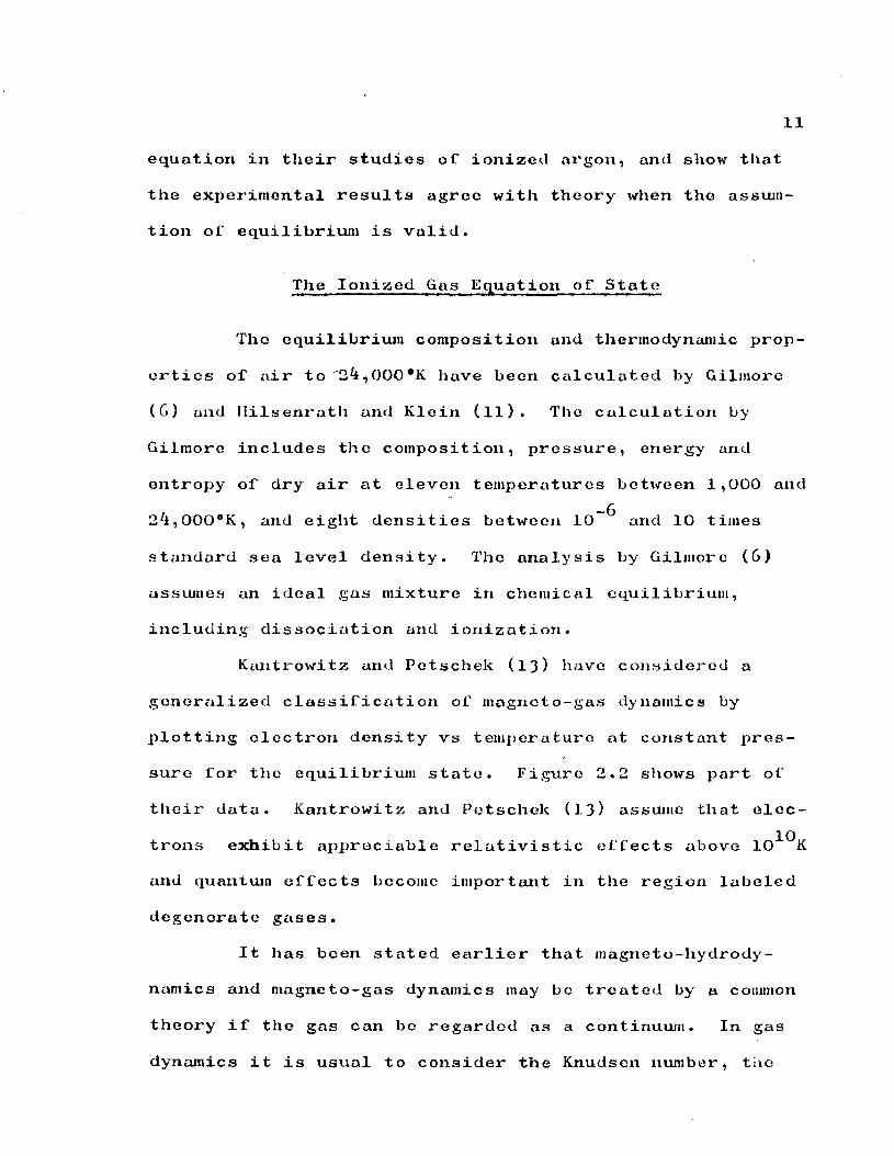
Figure 2.1 shows the composition of air at very
high temperatures for standard sea level density. It can
be seen that dissociation of neutral molecules of nitrogen
and oxygen becomes significant near 3000°C and ionization
of nitrogen atoms becomes significant around 10,000°C and
oxygen, 15i000°C. For lower densities ionization will
begin at lower temperatures (not shown).
Dissociation occurs when the energy of the internal
degrees of freedom becomes sufficient to overcome the
binding energy holding the atoms together. Equilibrium
dissociation is achieved when the rate of dissociation of
Page 18
8
o
o +> at
CM
o
© H a •H +>
& \ to © rl O •rt +•
-1 Temperature x 10 *C
Figure 2.1 Composition of Air at Atmospheric Density-
After Hilsenrath euad Klein (11)
Page 19
the molecules into atoms is equal to the rate of recombina
tion of atoms into molecules. The rate of dissociation or
ionization will be proportional, as a first approximation,
to the number of collisions occuring between molecules and
atoms which have sufficient energy to cause dissociation or
ionization. There is a characteristic relaxation time
which depends 011 the time necessary for the energy that is
added to the translational degrees of freedom of a molecule
or atom by collision to become distributed among all of the
degrees of freedom of the molecule or atom. For example,
although a molecule receives sufficient energy for dissoci
ation by collision, the molecule does not dissociate until
the energy of the vibrational degree of freedom reaches a
sufficient value to overcome the binding forces holding the
atoms of the molecule together. Measurements on argon by
Lin, Resler and Kantrowitz (lG) have shown that argon
reaches ionization equilibrium in the order of ten micro
seconds following maximum luminosity for temperatures
greater than 11,000°K.
Degree of Ionization
The degree of ionization of a gas in equilibrium
may be predicted from a thermodynamic argument. Saha (21),
in 1920, first presented a relation for a gas whose atoms
are ionized by losing only one electron, i.e., a singly
ionized gas. Saha has assumed that a singly ionized gas
Page 20
10
can be regarded as being in a state of dynamic equilibrium
represented by a completely reversible reaction of the
f orm,
A = A+ + e - Q±, (2.1)
whore A represents a neutral atom, A+ a singly ionized
atom, e the electron removed from the atom, and the
ionization energy. Based on this equation Saha applied
Nernst's equation to air in ionization equilibrium, re
sulting in the expression,
2 * 0 p = 3*16 X io"V/2
e x p ( _ Q./kT), (2.2) 1-x" 1
where P = total pressure, atoms,
T = temperature, deg. K,
= ionization energy, ergs,
x = degree of ionization, diniensionless,
k = Boltzman's constant = 1.3^0 x 10 ergs/deg.,
which has come to be known as the Saha equation. In many
practical problems the degree of ionization is sufficiently
small to justify the simplifying substitution of unity for
o 1-x" in the equation 2.2.
Von Engcl (5) states that there is ample evidence
obtained indirectly from investigations on arcs which sup
ports the view that tho thermodynamic treatment of Saha is
justified. Lin, Resler, and Kantrowitz (l6) use the Saha
Page 21
11
equation in their studies of ionized argon, and show that
the experimental results agree with theory when the assuin-
tion of equilibrium is valid.
The Ionized Gas Equation of State
The equilibrium composition and thermodynamic prop
erties of air to''24,000*K have been calculated by Gilmore
(G) and Hilsenrath and Klein (ll). The calculation by
Gilmore includes the composition, pressure, energy and
entropy of dry air at eleven temperatures between 1,000 and
24,000°K, and eight densities between 10 and 10 times
standard sea level density. The analysis by Gilmore (G)
assumes an ideal gas mixture in chemical equilibrium,
including dissociation and ionization.
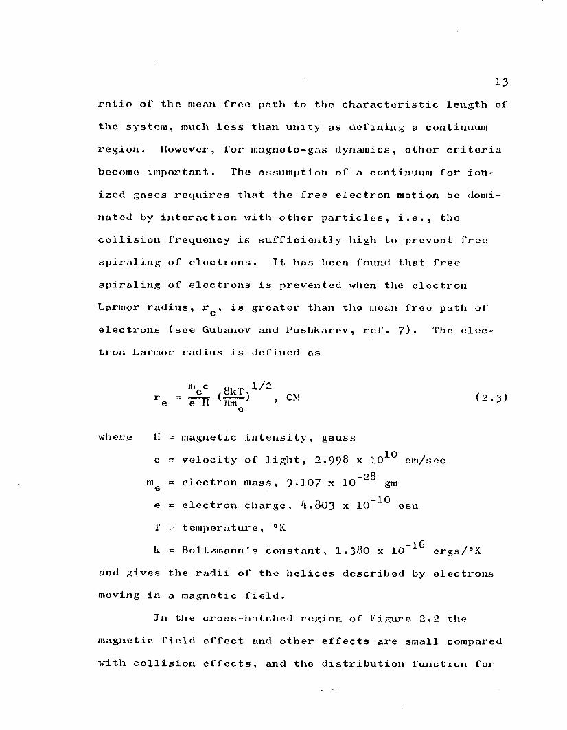
Kantrowitz and Petschek (13) have considered a
generalized classification of magneto-gas dynamics by
plotting electron density vs temperature at constant pres
sure for the equilibrium state. Figure 2.2 shows part of
their data. Kantrowitz and Petschek (13) assume that elec
trons exhibit appreciable relativistic effects above lO^^K
and quantum effects become important in the region labeled
degenerate gases.
It has been stated earlier that magnet o-liydrody-
namics and niagneto-gas dynamics may be treated by a common
theory if the gas can bo regarded as a continuum. In gas
dynamics it is usual to consider the Knudsen number, the
Page 22
10 12 3
L°gio Temperature in eV
Figure 2.2 Electron Equilibrium Diagram
P ^ 2n kT e
After Kantrowitz and Petschek (13)
Page 23
ratio of the mean free path to the characteristic length of
the system, much less than unity as defining a continuum
region. However, for magneto-gas dynamics, other criteria
become important. The assumption of a continuum for ion
ized gases requires that the free electron motion be domi
nated by interaction with other particles, i.e., tho
collision frequency is sufficiently high to prevent free
spiraling of electrons. It has been found that free
spiraling of electrons is prevented when the electron
Larmor radius, re, is greater than the mean free path of
electrons (see Gubanov and Pushkarev, ref. 7)« The elec
tron Larmor radius is defined as
n'~c Ki^r 1/2 re ' T T l (n5T> • CM (2"3>
where II - magnetic intensity, gauss
c = velocity of light, 2.99$ x 10"^ cm/sec
- 2 8 = electron mass, 9*107 x 10 gm
e = electron charge, 'i.8G3 x 10 esu
T = temperature, °K
k = Boltzinann's constant, 1.3^0 x 10 ergs/°K
and gives the radii of tho helices described by electrons
moving in a magnetic field.
In the cross-hatched region of Figure 2.2 the
magnetic field effect and other effects are small compared
with collision effects, and the distribution function for
Page 24
particles will be close to a Maxwellian velocity distribu
tion as in. a neutral gas. In this region, where r > mfp,
the electrons will drift through the ionized gas in a manner
analogous to the diffusion of neutral molecules, and the
assumptions indicated in the following section on the elec
trical conductivity are valid. This region is the region
of prime importance in this jjaper.
The "perfect gn.s" equation of state for a dissoci
ated or ionised gas in equil i br iiiin ,
( 2 - " > i
where R = universal gas constant,
8 . 31'136 x 10^ ergs/mole-°K ,
P = pressure, dynes/cm",
T - temperature, °K,
p - density, gni/cin ,
n^ - particles per atom,
M - atojnic weight,
is used by Gilmore (6) in calculating the composition of
air to 2'i,000°K. In using equation 2.4, M is the atomic
weight, l'i. 5yt9 for uir , since the n^ are defined as parti
cles per (air) atom. The chemical composition will be
essentially constant for a slightly ionized gas and a
highly ionized gas, and equation 2.4 taJtes on an even
simpler form since the terms n. will be constant. 1 1
Page 25
An equation of state for ionized hydrogen has been
developed by Williamson (27)? ns
kT 1/2H
1 - 0.01^0 p/ioo
(T/107)3
1/2 (2.5)
•2'i where H = proton mass, 1.673 x 10 gm,
Kaeppcler and Qaumann (12) give the following equa
tion of state applicable to any degree of ionization, any
gas, and any density.
kTIN. x
l
1 -
O e~r 6€kT
VN.x. f ( r a . ) L s i i i
where
£
r = j^Tie2 £ N±x?/lcT ^ 1/2
( 2 . 6 )
f(ra. ) = 1 - —rr ra, + 263 I I *
-10 c = electron charge ('i.802 x 10 e.s.u.),
N. - density, ions/cm ,
x. = valence, 1 '
a. = ion radius, cm, x ' 1
-l6 k = lioltzmann1 s constant (I.38O x 10 ergs/°K),
T = temperature, °K,
6 = permittivity, esu.
Williamson's equation of state for ionized hydrogen, equa
tion 2.5, is contained in the equation of state by
Kaeppeler and Baumann (12), equation 2.6, as a special case.
Page 26
16
Hilsenrath and Klein have shown that the correction
to the "perfect gas" equation of state is less than four
percent for ionized gas when the density is less than
standard sea level. Since the physical region of interest
for this problem is the region of low density (10~^
atmospheres or less) it appears reasonable to use the
"perfect gas" equation of state.
Electrical Conductivity
The electrical conductivity of ionized gases depends
on the diffusivity of electrons in the gas. At low degrees
of ionizfitiori, the diffusivity depends primarily on the
cross section of electron-atom collisions. At high degrees
of ionization, the diffusion is limited by the long range
Coulomb forces.
For a slightly ionized gas Lin, Resler and
Kantrowitz (l6) developed the following expression from
measurements of electrical conductivity:
CT = 0.532c2 x/ (mekT)1/2qa, , (2.7)
where q = electron-atom cross section, a
e =• electron charge, e.s.u.,
in = electron mass, e '
x = degree of ionization (equation 2.2),
k = Doltzmann's constant,
T = temperature, °K.
Page 27
For a highly ionized gas, Spitzor and Harm (23)
developed the expression
G~d - 0.59l(kT)3/2/mt//2o"ln(h/bo) , (2.8)
where e » electron charge, e.s.u.,
h = Dobyc shielding distance,
= (kT/87lNee2 ) 1//2 , cm,
O b - impact parameter - e^/OkT, cm,
O - iinuact oarnmeter - e
3 N -- electron density, electrons/cm . e
Lin, et al, found good agreement for all ranges of
ionization levels if these two conductances (equations 2.8
and 2.7) were treated as conductances in series. Thus
cr = 1.88(m kT)J1.69m 1^"e"ln(h/b )
e a e o 2 + Z372
-1
. ( 2 . 9 ) xe (1<T)
While the first term in equation 2.9 appears to vary
inversely with the temperature, the degree of ionization,
equation 2.2, is a strong function of the temperature and
hence, the electrical conductivity increases with an
increase in temperature.
Recent test data reported by von Karman (15) shows
2 that the electric conductivity varies inversely as M in
the region behind a shock wave for Mach numbers ranging
3 from about six to eighteen and inversely as for Mach
numbers ranging from eighteen to thirty. This appears to
Page 28
18
be consistent with equation 2.9 in that the Mach number is
inversely proportional to the one-half power of the temper
ature .
Viscosity
The general formulae for the first approximation to
the viscosity and thermal conductivity in the absence of
external forces have been evaluated by S. Chapman (k) for
a completely ionized gas and by L. L. Moore (19) for mod
erate temperatures. The coefficient of viscosity can be
expressed as
U T N jj- = <!-) (2.10) ^i i
where |JL = coefficient of viscosity,
T = temperature,
and ( ). = reference state. l
The value of exponent, N, varies with the temperature. For
moderate temperatures, Moore predicted the value of N to
range from one half to three halves. At extreme tempera
tures where ionization is essentially complete, Chapman
found the value of N to be five halves.
N = 1/2 for moderately low temperatures,
= 3/2 for moderately high temperatures,
= 5/2 for extremely high temperatures. (2.11)
Page 29
19
If N is treated as a linearly varying function of
the degree of ionization, that is,
N = 1/2 + 3/2 x (2.12)
the error in predicting the coefficient of viscosity was
less than four percent when the calculated value was com
pared with those presented by Moore (19) and Chapman (4).
Thus, for this analysis, it is assumed that
.. T 1/2 + 3/2 x £ = (£-) (2.13) ^ i
Thermal Conductivity
The first order variation of the coefficient of
thermal conductions closely parallels the variation of the
coefficient of viscosity. The variation can be expressed
as
A <T> ^ ~ = (?-) (2.14) Al Ti
where A - coefficient of thermal conduction,
T = temperature,
and ( ) = reference state.
As with the coefficient of viscosity, the exponent, N,
ranges from one half to five halves. For this analysis, it
is assumed that
A - 1/2 + 3/2 x 7T" = (2.15)
Page 30
20
Prandtl Number
The Prandtl number is defined as
Pr = —Z- (2.16) A
The viscosity and thermal conductivity for a gas have been
presented in previous sections. The specific heat of a
highly ionized gas was approximated by Chapman (4) as
cp = !s- (2-i7)
1
where k = Boltzman's constant,
and m. = ion mass. x
The specific heat for a raonatomic gas (a dissociated gas)
can be approximated by
C P = I I ( 2 - l 8 )
where k - Boltzman's constant,
and in = atomic mass.
von Ka'rman (15) demonstrated that, in the area of magneto-
aeronautics", the variation of the Prandtl number can be
based on the amount of ionization. von Karinan obtained the
empirical expression
= 1 - x (2.19) <0
where Pr^, = 0.721
and x = degree of ionization (equation 2.2),
Page 31
21
5 for temperatures less than 5 x 10 #K. Equation 2.19 is
used in this analysis.
Region of Interest
While the general region of interest is the one of
a continuum, the cross-hatched region in Figure 2.2,
specific interest for this analysis was restricted to the
region of aerodynamic flows. Mach numbers in the neighbor
hood of fifty can produce stagnation temperatures of
approximately 55,000#K or 5 ©V. An additional vertical
line can be added to Figure 2.2 to further restrict the
area of interest (not shown).
In this area, two effects, that of radiation and
species diffusion, can be neglected. Several authors have
recently considered the effects of radiation with respect
to the flow variables. Energy radiated per unit volume
for the region of interest has been shown by B. Kivel (von
Karman, lk) to have a maximum value of about 10 watt-
sec/cm . The kinetic energy of a unit volume entering the
boundary layer will be converted to thermal energy when
the fluid velocity is decreased. The kinetic energy is a
function of the initial velocity and ranges from approxi-
3 mately 200 to 1000 watt-sec/cm in the region of interest.
For maximum radiation and minimum energy the maximum error
due to neglecting the radiation term in the energy balance
is on the order of 3%•
Page 32
22
Braum (3) discussed the contribution of species
diffusion for various regions of interest. In his analysis,
a distance over which diffusion would be significant was
defined. For the case of the stagnation boundary layers,
that is the case of the maximum thermal gradients relevant
to flow analysis, the distance for which an excess charge
density resulting from species diffusion was shown to be
on the order of 5 times the mean free path of the gas.
Thus on a macroscopic scale the effect of diffusion is not
significant.
Page 33
CiLAPTER III
EQUATIONS OF MOTION
Electromagnetic Equations
A tabulation of the macroscopic equations of elec
tromagnetic theory is given below for convenient reference.
D = 6 E (3-1) e
n - ven (3.2)
V-d = p Q (3.3)
V'B = 0 (3.4)
VxE = -dB/et (3.5)
Vxn = n. (T -t- 3D/at) (3.6)
I11 addition, Ohm's Law may be written as
J = C7(E + q x D) + peq (3-7)
Continuity Equation
The continuity equation for continuum magneto-gas
dynamics requires no additional electromagnetic terms and
is the same as that for a neutral gas.
23
Page 34
2'l
a"4 + V*(/0q) = 0 (3.8)
Momentum Equations
The momentum equations consist of the usual Navicr-
Stokes equations plus electromagnetic force terms due to
the motion of a conductive fluid tlirough magnetic lines of
force and due to excess charge density in the fluid. The
latter effect, that of forces due to the excess charge
density, will be neglected.
dynamics consists of the usual terms as written for a
neutral gas plus the heating effects due to the electro
magnetic actions and the energy stored in the field.
= " V P + + J'b ( 3 • 9 )
Energy Equation
The energy equation for continuum magneto-gas
Rrrr - 'jrr- + V.(wf) + <§> + q-Jxli (3-10)
wh ere
<#> - (211 + lJ^ ) (^' q)2
O 2 o
(3 -11)
Page 35
In order to obtain a unique solution to the prob
lem, it is necessary to have the same nujnber of equations
as dependent variables.
In a three dimensional problem the fifteen dependent
variables are three components of the magnetic flux, three
components of the elcctric flux, three components of the
electric current, three components of the fluid velocity,
the fluid pressure, the fluid density, and the fluid
temperature. The corresponding fifteen independent equa
tions are six scalar equations obtained from Maxwell's
equations, three scalar equations obtained from Ohm's Law,
the equation of continuity, the three scalar momentum equa
tions, the energy rate equation, ami the equation of state.
In addition, an equation is necessary for each fluid prop
erty which is allowed to vary, i.e., the coefficients of
viscosity and electrical conductivity.
Certain other variables are used in this paper for
convenience but can be expressed in terms of the dependent
variables listed above, i.e., the Mach nutnbor and the
Reynolds number. With the set of fifteen equations in
volving fifteen dependent variables together with appropri
ate boundary conditions the problem is mathematically
determinant.
Page 36
CHAPTER IV
MODEL
Statement of Model
The problem under consideration is the solution for
the flow par,line tor s for flow of an ionized gas over a flat
plate with a constant magnetic field applied perpendicular
to the plate.
The following assumptions are made:
1. The fluid is treated as a continuum.
2. The free stream velocity is parallel to the plate.
3- The flow in all regions is in a steady state.
k. The flow near the plate (i.e., y < ) is a laminar,
two-dimensional flow.
5. The flow outside the boundary layer is inviscid.
6. The applied electric field is zero.
7- The magneto-gas dynamical effects are confined to
a region bounded by the plate and a Mach wave
originating at the leading edge of the plate.
The last assumption is arbitrary. In the case of an actual
body the bow shock wave would be the logical outer boundary
for magneto-gas dynamical effects. As the body thickness
becomes infinitesimally small, i.e., a flat plate, the bow
26
Page 37
shock wave is replaced by the Mach line. Figure 4.1
represents the configuration for study.
General Floi? Analysis
It was first shown by Prandtl that the Navier-
Stokos equations can be simplified in regions where rapid
changes of variables occur essentially in a direction
normal to the main flow. When x is taken in the direction
of the main flow and the argument restricted to two dimen
sional steady flow, the governing equations can be simpli
fied by neglecting certain smaller magnitude terms resulting
from the sinallness of v and the small rate of change of all
quantities in the x direction as compared to their rate of
change in the y direction. The complete analysis leading
to the simplified equations for two dimensional steady flow
has been treated in Schlichting (22, chapter XIV) with the
exception of the electromagnetic terms. Only the electro
magnetic terms will be considered in detail here.
The continuity equation, equation remains un
changed from that given by Schlichting (22) for steady flow
Reduced Equations of Motion
i'i.l)
Page 38
28
Magnetic field,
Region 2 Inviscid Region 1
Free Stream
Region 3 Boundary Layer
Figure 4.1 Problem Model
Region 1: Free Stream Flovr with no magnetic effects
Region 2: Inviscid Flow with magnetic effects
Region 3: Boundary Layer Flow
Page 39
29
The x-momerituin equation from equation 3*9 is
/><u§ii + viH) = _ |£ + i-jxU + ( k . 2 ) ' <*x dy dx o y <?y
Using the assumption that the magnetic field is applied
only in the y direction and is constant in magnitude
JxD = -o"B"ui + higher order terms. (li. 3)
The higher order terms are discussed Inter. Thus the x-
momentum equation becomes
„ / d u d U * d P —r » 2 d / , < J U \ , . . , . P (u-r— + v-r—) - - —— -<rn u + -r—(p*—)+ higher order terms.
dx «y ox ®y dy
i k . k )
Likewise the y-momentum becomes
+ * " 3 7 + ( ' * - 5 )
where Y is the term resulting from JxD. It is desired to
withhold further analysis of¥ until later.
The energy equation, equation 3*10, can be expressed
as
+ *Sy> = 41 +$ + (4.6)
Under the assumption in the Statement of Model, the
magnetic contribution can be expressed as
2 2 q*(JxB) = <TD u + higher order terms. (k.7)
Page 40
30
Substituting equation 4.7 into equation 4.6, the final
expression for the energy rate equation becomes
+ higher order terms (4.8)
Order of Magnitude Analysis
Non-dimensional variables are defined in the
following manner:
u* = u/u , v* = v/u ,
X* = x/L, y* - y/L,
T* = T/(T -T^), W
P* = P/jgVI, (4.9)
The x-inonientuin equation, equation 4.4, with the
above substitutions can be written in the following form,
*du»- . ,du\ £P» CYiSL , yO#(U*T T + V * r r -) ^ J- - n U* ~ <5x* <3y* ax* /2o Uoo
1W- <3— (4.10) d y * ^ d y '
The coefficients of the velocity gradient and the velocity
appearing on the right hand side of equation 4.10 are
recognized as the reciprocal of the Reynolds number and the
Page 41
31
ratio of the square of the Hartniann number to the Reynolds
number respectively.
Reynolds Number, Re = jQ\iL/[i. (4.11)
Hartmann Number, Ha = , (4.12)
The ratio of the Hartmann number squared to the Reynolds
number is often called the magnetic influence parameter,
X = . (4.13) Re u
On the same physical basis as reference 22 one can
assign the order unity, 0(l), to the magnitude of u* and
x* and the order cT/L, 0(<T/L), to the magnitude of v* and
y * •
The x-momentum equation is then observed to bo the
following
u.*ul + = zl[i£l + _ 1_ * (u.£u•) 1 3x* dy* Re d y * dy* J
0 ( 1 ) 0(1) 0(1) ? ? 0(1) ? 0(L2/J2) (4.14)
Since the left hand side of equation 4.l4 is of order unity,
terms on the right hand side of the equation must be of
order unity or larger to have a significant influence on
the solution.
The following statements can now be made:
for viscous influence 0(Re) = 0(1^"/^""); (4.15)
Page 42
32
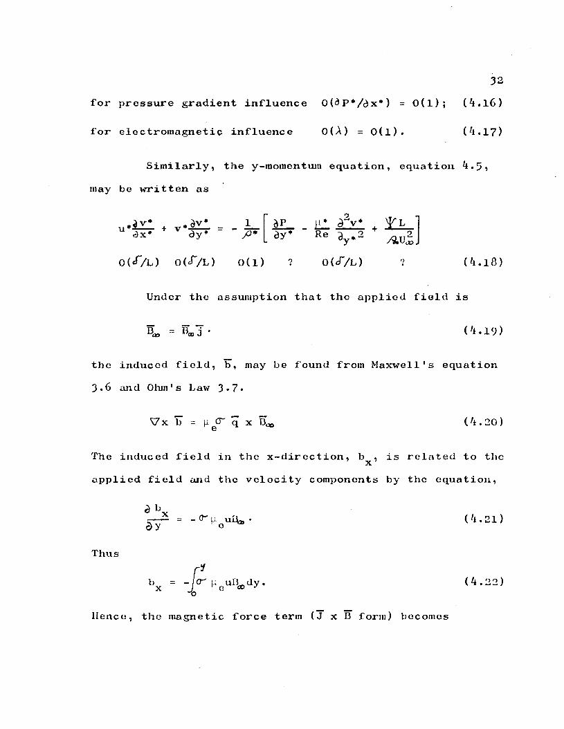
for pressure gradient influence 0 ( d p * / d x * ) = 0(l); (4.l6)
for electromagnetic influence 0(A) = 0(1)# (4.17)
Similarly, the y-moinentuin equation, equation 4. 5,
may be written as
U*S—_ + v*-2—— r3x* dy*
1 dy*
O(<T/L) O(<T/L) 0(1)
ILL a"v* + 1±
Re V2
0(cT/L) (4.18)
Under the assumption that the applied field is
(4.19)
the induced field, b, may be found from Maxwell's equation
3.6 and Ohm's Law 3-7»
S7 x b - (i CT q x ( 4. 20 )
The induced field in the x-direction, b , is related to the x'
c\pplied field and the velocity components by the equation,
3 b
dy ou4a> (4.21)
Thus
r* b = - CT }i uD dy. (4.22) x J e <® J
-x>
Hence, the magnetic force term (J x B form) becomes
Page 43
33
CT (qx(B«, + b) ) x (D^ + b) = i r( -B^u+vB^b )
+ j^-vb^+ul^b ) . (4.23) X
Thus
i-(J x II) - CTB^u + 0(<T2/L2), (4.24)
and
J. (J x U) = <rbxul\, + OiS*/Lh. (4.25)
From equation 4.22, 0(b) is no larger than an order of
<f/L. Returning to equation 4.5?
y = <r bxBBu , ( 4 . 26 )
and
= Au*b* (4.27)
.on which is no larger than order S/L. Using this in equati<
4.18, and comparing the various terms in the equation, it
may be observed that the pressure gradient in the y-direc-
tion, d P*/dy* , is of 0(cT/L). Since is of an order
larger than dP'/dy*, wo may assume that the pressure varies
only along the x-axis and treat c)P*/dx* as a total deriva
tive. When the pressure variation is thus restricted, the
pressure in the boundary layor region may bo determined by
the boundary conditions at the outer edge and hence the
number of unknowns is reduced by one. This fact allows us
Page 44
3^
to reduce the number of equations by one. Since the y-
momentum equation is an order of magnitude smaller than the
other equations, it is chosen to be the one which is not
considered.
Similarly the energy equation in dimensionless form
inay be written as
1 1 * + V • • — • d x * d y * / * *
1 *2 ^ dP* • A _A_ d2T* Re dx» U PrRe .2
dy' .
0( 1 ) 0 ( 1 ) o ( i ) o( i ) o( i ) ? o ( l 2 / c f r 2 )
(4.28)
where <Tt is the thermal boundary layer thickness and
u^/c (T - T ) , (4.29) 9 T1 W CO 1
Pr - p Cp/k. (4.30)
For convenience U, c , and k have been considered to be p
constant witliin one order of magnitude in equation 4.28.
The following statements may now be made:
for heat generation influence 0(E) ~ 0(l); (4.31)
for conductive influence 0(l/PrRe) = 0(S^/h^). (4.32)
In the case of a gas, the Prandtl number is nearly
unity. Comparing equations 4.32 and 4.15, it is observed
Page 45
35
that the thermal boundary layer is of the same order of
thickness as the velocity boundary layer,
o( ,T t ) - o(cT) . (4 .33)
Discussion of Model
The model can now be written in terms of applicable
equations for the three regions of flow.
Region 1. Free stream
The various variables from this region (i.e., M^,
, etc.) arc used as boundary conditions.
Region 2. Inviscid flow
The various variables are assumed to be actcd upon
by the magnetic field. However, the flow is assumed to
be one dimensional, without shear and with negligible
thermal conduction. The use of these assumptions
allows further reduction of the equations of motion.
The resulting equations of motion for Region 2 are
1. Cont inuity
d 7 (p0 u 0 ) ~ 0 j Ci.j'i)
ax
r)u o o o = cos)
if A subscript 0 will be used to denote the flow variables in Region 2.
Page 46
36
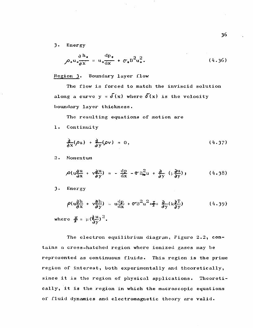
3« Energy
<3 h a ^P o o o / > o U „ — - + < r 0 o " u 7 . ( k . 3 6 )
Region 3« Boundary layer flow
The flow is forced to match the inviscid solution
along a curve y = cT(x) where <T(x) is the velocity
boundary layer thickness.
The resulting equations of motion are
1. Continuity
= 0 , ( 4 . 3 7 )
2. Momentum
+ Va7) = " S "<rB*u + I7 (4-38)
3. Energy
f(uf* + v|2i) = u^ + CTD2u2+f+ j-(k|l) (4.39) ' <3x dy dx <^y (?y
where
The electron equilibrium diagram, Figure 2.2, con
tains a cross-hatched region where ionized gases may be
represented as continuous fluids. This region is the prime
region of interest, both experimentally and theoretically,
since it is the region of physical applications. Theoreti
cally, it is the region in which the macroscopic equations
of fluid dynamics and electromagnetic theory are valid.
Page 47
Experimentally, ionized gases, which Tall in the region
where the continuum assumption is Vcilid, are naturally
easier to obtain because of the proximity of this region to
the region of a continuous neutral gas. Lysen and Serovy
(l8) give an extensive review of the typos of problems that
can be treated, based on the assumption that the fluid may
be represented as a continuum.
The phenomena of viscous interaction in the flow
over a flat plate has been discussed at great length in the
literature, e.g., Schlichting (22). For flow of a real «
fluid, i.e., 011c with viscosity, the flow is retarded
primarily in the vicinity of the body surface. This region,
called the boundary layer, is observable. While many
definitions of the boundary layer thickness are used, the
most physical definition is the one based on the mass flux
defect, called the displacement thickness, J*- The inviscid
flow outside the boundary layer sees a body which is
represented by the physical body plus the displacement
thickness. The effective change in the shape of the body
gives rise to the body shape factor, p. Tho velocity
boundary layer thickness,cT, the thickness for which the
local velocity is equal to tho free stream velocity, has
been previously defined.
It will be assumed that the velocity and thermal
boundary layer thicknesses are equal. While this is true
only if the Prandtl number is unity, it is considered a
Page 48
first approximation when the Prandtl number is of order
unity. Bogdonoff and Hammitt (2) concluded that the error
introduced by this assumption may be as great as 50% for
the thermal boundary layer thickness but is insignificant
for the boundary layer thicknesses related to momentum.
Page 49
CHAPTER V
INVISCID FLOW SOLUTIONS
Equations of Motion
Based upon the assumptions made in Chapters II
(Ionized Gas) and IV (Model), the equations of motion for
region 2 may be written as
1. Continuity
(/3.u0) = 0 (5.1)
2. Momentum
du# dp, = - dT" - <5-2>
and
3. Energy
dh® dp.
/° •U*d^~ = U#dF" + <r'^oU° * (5*3)
Density and Pressure
The equation of continuity may be integrated
directly. Applying the boundary conditions from the free
stream flow, we have
(O„U0 = PaPtjo* (5-^)
39
Page 50
ko
Solving for the density ratio
P*>
u CO
U. (5.5)
From Chapter II we may write the pressure ratio as
p. p.h. (5.6)
Substituting for the density yields
00
ucb h.
uc h^ (5.7)
Enthalpy
To obtain an enthalpy profile for the inviscid
region it is necessary to solve the energy equation 5*3 •
Differentiating equation 5»7 with respect to a dimension-
less length, x*, yields
dP.
dx* ~ P*>
u 00 1
• "-no
dh. du0
u. dx*-(5-8)
and with use of equation 5-3 1
dh# £/|dho
dx* ~ ^ [dx*
h- du,
uc dx* A. u. (5-9)
or
1_ h.
dh.
dx*
du = - -r~°W +
u. dx* • (5.10)
From the section on electrical conductivity we may write
Page 51
4l
(5.11)
Then, integrating equation 5*10 yields
h. u. tf-1 ln(^—) = -ln(—) + fltf-l) /IXx* (5*12)
or
^ • u^l-jr p _ _ jj- = (—) exp [ J f(/-1) (5.13)
Velocity
By using equation 5*10 in connection with 5»8 we
may solve the momentum equation 5*2 for the velocity pro
file. Writing equation 5.2 in a non-dimensional form gives
dCuo/u^)
dx*
dp # u,
n 2 dx P» uD
(5.14)
However, combining equation 5*8 and 5*10 results in
dp. -r—r = JR. =-dx * ® he
h. u«, u.
(<r-I) Xm M£ -uoo d(u./u^)
u. dx' (5.15)
Substituting 5»15 into 5«1^ and solving for d(u#/u^,)/dx*
gives
dfu./u ,)
dx*
y
(M^-l) u„ ( 5 . 1 6 )
Page 52
42
In the following section it is shown that M# may be ex
pressed as a function of x* only (see equation 5*23)•
Hence, for the purpose of computer integration, we may
•write
u
u
0
- = exp (-*/!«, M*0 ). (5-17) 07 4> M;-I
Mach Number
The logarithmic differential of the square of the
Mach number is
, m 2 , 2 . 2 dM du da / c i «\
= ~2 2~ * (5,l8) M u a
However,
^ = F1 ' <5-19) a
and
^ ' (5-20) u
Thus
dM^ du, dh0
—tt- = 2 . (5*21)
Page 53
43
Combining equations 5•21, 5•10, and 5»l6 yields,
, 2 i i f l / t . M . v „
dx* . (5.22) dM
M
n.HB2 2 •
Using the expression for A #, given in equation
5.11, we can integrate equation 5*22 to obtain
' 6 - 1 m 2 "I m2 2 • ^ ~ © r «i 2 *i
y—T 2 —P = exP -2MKM,#- . (5.2 3) 1+ 2- =- M M L J A 2 ® J •
Summary of Inviscid Flow
In this chapter the following relationships have
been established:
p.
K
U c
U „ (5-24)
u*> h.
U, hw
h. u. 1-lC r
j- = (—) exp [ W-l) g] ,
U ,
u„ = exp
i+ 41
- /
iii 2 TT MI
J dx*
X M?-l
i+ >u2, M
(5.25)
( 5 . 2 6 )
(5.27)
= exp [-2 If ^o>M* j£j . (5.28)
Page 54
These five relationships will be used in the fol
lowing chapter as the boundary conditions for the outer
edge of the viscous boundary layer flow of Region 3»
Numerical examples are presented in Chapter VII.
Page 55
CHAPTER VI
PROBLEM SOLUTION
General Method
The method of solution of the flow variables is one
of obtaining a finite difference equation for the boundary
layer thickness which may then be solved by computer tech
niques. The momentum and energy equations will be put in
integral forms. Before these two equations can be further
developed it is necessary to establish a velocity profile.
After the method of Pohlhausen, a polynomial will be used
to represent the velocity profile. While this method
satisfies the boundary conditions, it does not satisfy the
momentum equation throughout the boundary layer region.
However, since the integral form of the momentum equation
is used, knowledge of the exact solution for the velocity
profile is not necessary. Schlichting (22) compared
Pohlhausen's solution with the so called "exact" solutions
for the ordinary case and found the error to be very small.
The outer boundary conditions for the boundary
layer region will be based on the inviscid flow solutions.
It will be assumed that the only pressure gradient is that
induced by the magnetic field.
^5
Page 56
46
The resulting analysis yields a differential equa
tion for the boundary layer thickness coupled to other
equations involving the outer boundary conditions and wall
conditions. A solution is then obtained by use of a dig
ital computer.
Velocity Profile
The ratio of u to u, is assumed to be a polynomial
function of T| •
( 6 . 1 )
where T\
and a, b, c, d, and e may be functions of x
The boundary conditions are
y = 0 u = v = 0 o r f ( O ) = 0 ; (6.2)
u u or f(l) - 1; (6.3)
r 3u „ y = ay or f (1) = 0; (6.4)
or f''(1) = 0. (6.5)
By considering the momentum equation at the wall, a
fifth "boundary condition" may be determined.
Page 57
^7
^ |u} = dP (66)
'w d 2 , , dx >5
y wall
Equation 6.6, with the use of equation 4fc»35i can be
written as
f''(0) = -P (6.7)
where
p = -p Re 4 "*#• " L
1 du» ^ 1
u7 "dx/ L + ' (6*8)
3 is the body shape factor discussed previously.
Since the velocity at the wall must vanish, no
constant terra may appear in equation 6.1 and hence, e must
be zero. Solving for the other coefficients appearing in
equation 6.1:
a = 2 + P/6, (6.9)
b = -3/2, (6.10)
c = -2 + 3/2, (6.11)
d = 1 - 3/6. (6.12)
Finally, the velocity profile can be written in the fol
lowing manner:
» f(n) = f(ti) + 3G(n), (6.13)
where
f(ti) = i - (i - n)'5(i + ti)» (6.i4)
Page 58
48
G(ti) = (l - r\) 3 /6, (6.15)
and 3 is defined in equation 6.8.
It is observed that the velocity profile reduces to
that given in Schlichting (22) for the case of no magnetic
field, \ = 0.
Momentum Integral
The momentum equation 4.38 can be solved for the
shear term and integrated with respect to y.
v i + CB u + '5~)t y (6.l6)
Consider the term on the left.
J h_ dy (^)dy = = li £«) (6.17)
<iy L dyL °dy „ ' w ay w ' ><r
Since 4^)r = 0, this term reduces to dy * '
J7>w = "rw • (6-l8>
From the continuity equation 4.37
°v = - J (pu)dy • (6.19)
Then
cT <T
j i d y = - J [|if (/lujdyjdy (6.20)
Page 59
^9
Integrating by parts yields
/ </*v§7>dy =• - J - u!^r] dy- (6.21) 0
J ->Q
It has previously been shown that
dP ^ • o £ = sr = - - ^B-u- • (6-22)
Substituting equations 6.l8, 6.21, and 6.22 into equation
6.l6 gives
•ST du.
+ u'dT ?- = / ru _ u i _ w J L *ax dx ^ dx
- ( 0
*u j dy • (6.23) O CO O uD
It is now possible to rearrange the terras in equation 6.23
to arrive at the following relationship,
dO O d u o r * 2 ^ • c f f - T w
n + l : s r ' 2 + i - - M " > + - T ^ = 7 ^ < 6 - 2 , » /*.u.
where
e = (^7a " S:)dy' (6-25>
'I (1 ~ Hh")dy' (6-26>
r*
and r = / (1 - ££-)dy. (6.27) •>b * *
Page 60
50
The definition appearing in equation 6.27 might be con
sidered as an electrical conduction thickness.
It may be observed that if the magnetic field is
zero, equation 6.2k reduces to the ordinary equation as
presented in Schlichting (22, Chapter XV).
Energy Integral
In a manner similar to that used for the momentum
integral, the energy equation can be placed in an integral
form. The energy equation 4.39 can be written in the fol
lowing manner
o
<T 9 r<f r*
dy + dy
A dh dP „2 2 + " Ud^ " CrB U . dy. (6.28)
Substituting as before for ysv and dP/dx and using the defi
nition of the Prandtl number, the energy integral can be
written as
H 2^U* ^ 2 d^(/'«u.h.9H) + Au.-gj- ©H +
• Ik $7] w + (6"29>
where
e « - -1 , d y ( 6 - 3 0 >
Page 61
e = f'L (1 - £»_>dy. r J0 U. (T«U, J
51
(6.31)
As before, equation 6.29 reduces to,the solution given by
Schlichting (22) if the magnetic field is set equal to zero
and if the wall is adiabatic.
The various boundary layer thicknesses can be found
by using the momentum integral equation, equation 6.2^, and
the energy integral equation, equation 6.29* together with
the inviscid solutions obtained in Chapter V. The momentum
integral as previously developed is
From Chapter II and the fact that d p / d y = 0, the
density can be expressed as a function of the enthalpy in
the boundary layer.
The shear stress, equation 6.18, with the use of the
velocity profile, equation 6.13, can be written as
Boundary Layer Thickness
dO dx
( 6 . 3 2 )
(6.34)
Page 62
52 I
Substituting for f (0) yields
/ w ^w Pw 1 L
/*«
(6.35)
The following terms may also be evaluated in terms
of P with the use of the velocity profile.
e_ „ f'sL_ (i . £-)dT, x J0 U. U. 77
, l Z _ . J r . j L (6. 3 6 ) 315 9^5 9072
A = io + P/12° (6.37)
Using equations 6.35* 6.36, and 6.37, equation 6.32 may be
written in the form
2_ €k 1£l t I SL i_ (2-M2) - i_ (2_ + _£_ )] cTx L dx l2 [ J- u. dx v •' u. dx v10 120 'J
^"l f h d U * . 3 / , uo- H/3* . /jv (2 + P/6) t 2 J [u» dx7L A'U dT1 ^./>, Re.
+
L" Jo
(6.38)
With the definitions
z = <f2/L2, (6.39)
1 -1 ^ o
K = ^7 ' (6-4o)
and K = K+/(., ( 6 . 4l)
equation 6.38 becomes
Page 63
53
dz dx/L = - S ir [fj* <To + T§o)+I]
^w /°w (1 + 13/12) //- / r,x + FT Re.e/^ (6-42)
where
1 = 5 I [ k ' + ( 1 - ^ d | i - ( 6 . 4 3 )
Once an expression for the density or the enthalpy is
obtained, equation 6.43 can be evaluated. Equation 6.42 is
an ordinary first order differential equation with variable
coefficients which, at least numerically, can be integrated,
Enthalpy Profile
At this point of the analysis it is useful to
restrict the problem to the adiabatic wall. Although this
prevents an analysis of the heat transfer at the wall, it
allows the dominating factor in the boundary layer flow to
be that due to the magnetic field.
For an adiabatic wall
i£) = 0. (6.44) 9 y J w
With this boundary condition and with the Prandtl number
equal to unity, the enthalpy may be shown to be a function
of the velocity component in the x direction.
Page 64
5 4
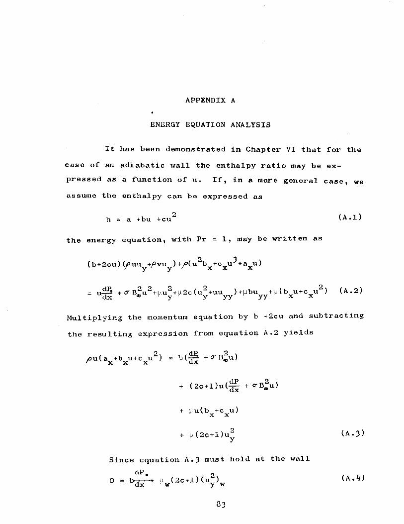
Assume that the enthalpy may be written as
h = a + cu^. (6.45)
Since the gradient at the wall is zero, equation 6.44, a
linear component need not be considered. The derivatives
of h are
= 2cuu , (6.46) dx x'
= 2cuu , (6.47) dy y'
2 and ^—77 = 2cuu + 2cu (6.48)
dy2 yy y
Substituting the above expressions into the energy equation
4.39 yields
dP 2 2 2 2cu(puu +pvu ) = u-r— + cr B n +|iu J x y y dx ® ' y
+ 2c|~i(u"+uu ). (6.49) y yy
If the momentum equation 4.38 is multiplied by 2cu and sub
tracted from the above equation we obtain
0 = u^'5x + l + 2c ) +|i ( 2c + l )u^. (6.50)
Since the modified energy equation must be valid at the
wall
c = -1/2. (6.51)
Page 65
55
Thus
h = a-u^/2. (6.52)
Applying the boundary condition,
h = h. at r\ = 1, (6.53)
= 1* (6.54) • U.
In the case Pr £ 1, a temperature recovery factor, r, must
be introduced. While the factor is a function of the flow
conditions, it has been shown by several authors (refer
ences 14 and 22) that the recovery factor is approximately
equal to the square root of the Prandtl number.
h _ jf - lv, 2_ 1/2/- U\ // rr> _ _ = 1 + y . l . - . - M t P r ( 1 - — ( 6 .55) U9
for an adiabatic wall.
The preceding method will not yield a solution if
the adiabatic wall restriction is released. Appendix A
contains the more general development showing that the
temperature (enthalpy) is a function of u alone only for
the adiabatic wall. In the general case the energy equa
tion is non-linear and is coupled with equation 6.42.
Drag Coefficients
The total drag on a body is comprised of two
contributions. The first is due to the viscous shear, T , w
Page 66
56
at the surface of the plate. The second is due to reaction
between the flow and the magnetic field.
The local shear force has been defined as
K - <^> • (6.56) J w
Then
0 = 1 • (6.57) f 1/2/O.u! w
In analyzing the effects of the magnetic field the ratio
of the magnetic skin friction coefficient to that of the
ordinary case will be used.
The total drag coefficient is defined as
* { %t(1 - »dy- (6-58)
It may be assumed that the effects of the magnetic field
are negligible outside the area defined by the body surface
and the bow shock wave for an arbitrary body. Since the
Mach line for a flat plate has somewhat of an equivalence
to a bow shock wave for an arbitrary body, the contribution
due to the magnetic influence will be restricted by the
Mach line. Hence the upper limit for the integral appear
ing in equation 6.58 is taken to be
y = L tan(sin"^(l/M^)). (6.59)
Page 67
57
Collected Equations
Thus far a set of coupled equations has been
developed for the adiabatic flat plate. Since closed-form
solutions are not obtainable, a digital computer was used
to obtain numerical solutions. The purpose of this section
is to present in final form the primary equations used in
writing the computer program. Because the symbolism used
in Fortran languages is limited and somewhat unique, the
symbolism used in this section will be consistent with the
preceding chapters and not with the computer program
appearing in Appendix B. The program is self-contained and
confusion in symbolism has been avoided as much as possible
by the use of comment cards.
a function of the ionization level and ranges from 1/2 to
5/2. It is assumed that the variation of n is linear with
the percentage of ionization.
The momentum integral, equation 6.^2, may be
written in the form
In Chapter II, it was found that the coefficients
of viscosity and thermal conductivity vary as hn where n is
-r- + P(x)z = Q(x) , (6 .60)
where
P(x) + I (6.61)
Page 68
58
and
Q(x) = (^)n 1T±- 1 + 3/12). (6.62)
Since P(x) and Q(x) are in parametric form, it is not
possible to obtain an integrating factor. Instead, the
Runge-Kutta method, Reference 10, for a finite difference
equation will be used. To the third power of dx the finite
difference equation for equation 6.60 may be written as
z(x+ x) = z(x) + (A1+4A2+A^)/6 (6.63)
where A ^ = [ Q ,(x)-P(x)*z(x)Jax (6.64)
ag = (q(x + ~)-P(x + 7j—)'[ z(x) + tjpj ] Ax (6.65)
and A^ = /q (x+ax) -P (x+ax) • [z(x) +2A^-A^ ] Ax. (6.66)
The following equations were used in the computer
program:
Inviscid Mach number, equation 5*28,
1 + I z . 1 TTf 2
7TT = ° (6.67) 1 - 1 1 *2. l
Other inviscid parameters,
I2 CO
m;-I
du./u„ rvi; clx/L * <6.68)
:= (6.69) •A?
Page 69
59
( 6 . 7 0 ) p. u«> ho
" "7 •
Percent ionization, equation 2.2,
x2
—~ P = 3.l6xlO~7T5/2exp(-Q./kT) , (6.71) 2 - — - — *** 1 -x.
l
At this point in the solution the change in the Reynolds
number and the Prandtl number and the various gas properties
were computed. Also, the enthalpy at the wall was computed.
P = zKRe.(h/h.) (6.72) vr
u u.
= F(ti ) +(BG(ri) (6.73)
h = x + M2Pr1/2(l - ~) (6.74)
° u »
At this point the various gas properties were computed for
the boundary layer region.
dz dx
= -P(x)z+Q(x), (z =£2/L2) (6.75)
0/L = —- = V5 f( ( 3 ) (6.76)
Cd =
x/L tan (sin M
4rr (1 - ir)di <6>77) o u tp
e f T S ^ W ( 6 ' 7 8 ) /°,U. W
Page 70
6o
T hCD»
T7 = h7c~" (6-79) * * P
The size of the net is variable. Near the leading
edge the increment on x/L was chosen as 10~^ while after
10% of the plate length was traversed, the increment was
-3 increased to 10 « The former was chosen so as to reduce
any error resulting from the necessity of assigning initial
values to various parameters such as z and p. The latter
increment was chosen so that the truncation error would be
greater than or equal to the round off error. The increment
- 2 on T] was chosen as 10 for the same reason.
In addition to the equations listed above, several
consistency checks were incorporated in the program. The
two most important ones were the subsonic flow and separa
tion checks. When the inviscid flow reaches sonic velocity,
several changes in sign occur. The most obvious change
occurs in the exponential appearing in equation 6.67» If
the Mach number is less than unity, the exponential becomes
positive, as is readily seen from equation 5«22. The
condition for separation, the velocity gradient at the wall
being zero, implies that separation occurs for (3 = -12.
Once this value is reached or exceeded negatively, the
shear is no longer expressible as a linear function of the
velocity gradient. As a result, essentially no equations
Page 71
developed are valid. The most readily observable case is
the momentum integral equation, equation 6.17'
In general, the numerical solutions were obtained
by specifying the initial values of z and P, the various
gas properties for dissociated air, and the free stream
values for the Mach, Reynolds, Prandtl, and Hartmann num
bers along with the ratio of specific heats and the plate
length. While the information obtainable from the program
is essentially unlimited with respect to the problem,
certain variables present the flow solution. They are the
equations listed in this section together with the two
consistency checks discussed.
The flow chart, Figure 6.1, deraonstrates the steps
which the computer is required to follow. Three basic
operations are shown. They are: (l) input/output com-
-mands, which cause the computer system to read or write
information; (2) block processing, which causes the
computer to perform one or more arithmetic operations in
sequence; and (3) decisions, which cause the computer to
transfer to various block processing areas depending on
information which has been previously computed. Appendix
B containa the Fortran program written in standard card
format for Fortran.
Page 72
62
M (X) (Control \ Card
Data Card
-12
Ionization Level T/T ,T /T
-ubionic Reverae I Flow
Storage ,N(.l)
Output Data
Run Run + 1
STOP
LEGEND
^ Input/Output
0 Connection
0 Decision
D Processing
Figure 6.1 Flow Chart for Digital Computer Program
Page 73
CHAPTER VII
CONCLUSIONS
Physical Limitations
A number of assumptions and simplifications have
been made in order to obtain solutions to the problem
presented in Chapter IV. It is the purpose of this sec
tion to investigate the physical limitations as they affect
the range of application of the solutions.
In order to determine an approximate upper limit
for the Hartmann number, Ha, the variables appearing in
this dimensionless group will be considered separately,
von Karman (15) shows that the electrical conductivity of
air is about 1.5 mhos/inch for a flow at Mach 20 and a
density of 10 atmospheres, approximately an elevation of
59,000 feet. In the section on electrical conductivity it
has been pointed out that the electrical conductivity does
not vary greatly with density. Thus 1.5 mhos/inch will be
considered as an upper limit for a physically realizable
electrical conductivity for air.
The magnetic flux density which can be created in
the boundary layer will depend on allowable coil size,
power available, etc.; however, with a permanent magnet
2 1000 lines/inch (155 Gauss) is not unreasonable.
63
Page 74
64
A calculation for air viscosity versus temperature
for air by Moore (19) shows that slightly ionized air has
a coefficient of viscosity of roughly 10 slugs/ft-sec.
While the length of the plate is arbitrary, 60
inches is used.
In terms of the units given above
2 I'B^L2 1*8348x10 Mho/in) (B,lines/in2)2(L, in)2
p. (n, slugs/f t-sec)
(7.1)
Substituting the arbitrary maximum values defined
above
Ha Si 125 (7*2)
Since the solutions for the flat plate are based on
the assumption of laminar flow in the boundary layer, the
critical Reynolds number must be considered. When the air
stream is very free from disturbances, values up to 3 x 10
have been found for the critical Reynolds number (reference
22). Thus 10^ may be considered as a reasonable upper
limit for the Reynolds number.
In developing the equations of motion, it has been
assumed that the ionized gas is a continuous fluid in order
to apply the macroscopic equations of fluids and electro
magnetic theory to the problem. Tsien (26) suggests that
the realm of continuum gas dynamics may be assumed if the
1 /2 order of Re /M is about 100 or greater. Assuming a
Page 75
65
maximum Reynolds number of 3 x 10 limits the Mach number
to about 18.
Example Problem
In the limiting case of zero magnetic field, i.e.,
Ha = 0, the solution of the flow characteristics for an
ionized gas over a flat plate has been found to reduce to
the results presented by Schlichting (22) and von Karman
(14).
In order to present the effects of the various
parameters involved in the problem the following values
have been selected as typical for the free stream condi
tions :
m : 5, 15;
5 6 Re: 10"% 10 ;
Pr: 0.721, l;
Ha: 0, 10, 50, 100.
For the purposes of comparison, the following variables
have been held constant:
IS = l.k
& = ° -applied
While solutions for all combinations of the above variables
are not presented in the following pages^ sufficient combi
nations are included to demonstrate the results. It should
Page 76
66
be noted that because of the physical limitations presented
earlier some combinations are not valid.
Figures 7*1 and 7*2 (plots begin on page 71) pre
sent typical solutions for the inviscid flow region. The
Mach number and the velocity decay exponentially with dis
tance along the plate while the temperature, density^ and
pressure increase. Figure 7*1 demonstrates the fact that
for higher Mach numbers a greater influence is exerted by
the same magnetic field because of the increase in elec
trical conductivity due to the increase in temperature.
Particular notice should be made of the adverse pressure
gradient shown in Figure 7«2. Further comment on this will
be made in connection with body shape factor and separation.
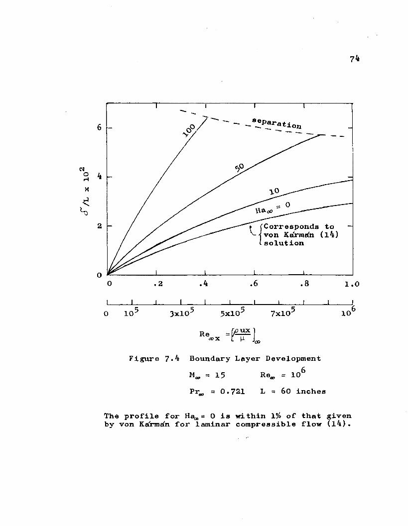
Figures 7«3 and 7,k show the effects of the magnetic
field on the boundary layer thickness for of 5 and 15
for constant Reynolds and Prandtl numbers. The variation
of the boundary layer thickness with the Reynolds number is
similar to that of ordinary flow, i.e., tT« 1/ -Vlfe. The
boundary layer thickness increases with the Hartmann
number, as might be expected by the adverse pressure gradi
ent, causing the velocity gradient at the plate surface to
decrease and thus decreasing the skin friction coefficient
as shown in Figure 7«5« This is consistent with the effect
Rossow (20) predicted for the case of no pressure gradient
and incompressible flow and is consistent with ordinary
flow as presented by Schlichting (22, Chapter XV).
Page 77
67
The overall drag coefficient has been defined in
terms of the wake drag. Since the upper limit of the
integral appearing in equation 6.73 has been taken as the
Mach line it is necessary to insure that the boundary layer
thickness is less than or equal to Ltan|i at x = L. The
computer program incorporates a check routine to insure
this condition is met. The contribution due to the magnetic
influence in Region 2 is approximately two percent of the
contribution from the boundary layer, Region 3> for each
additional increment of cT. In the cases considered the
upper limit was approximately three times the value of S'.
Figure 7«6 shows the variation of the overall drag coef
ficient .
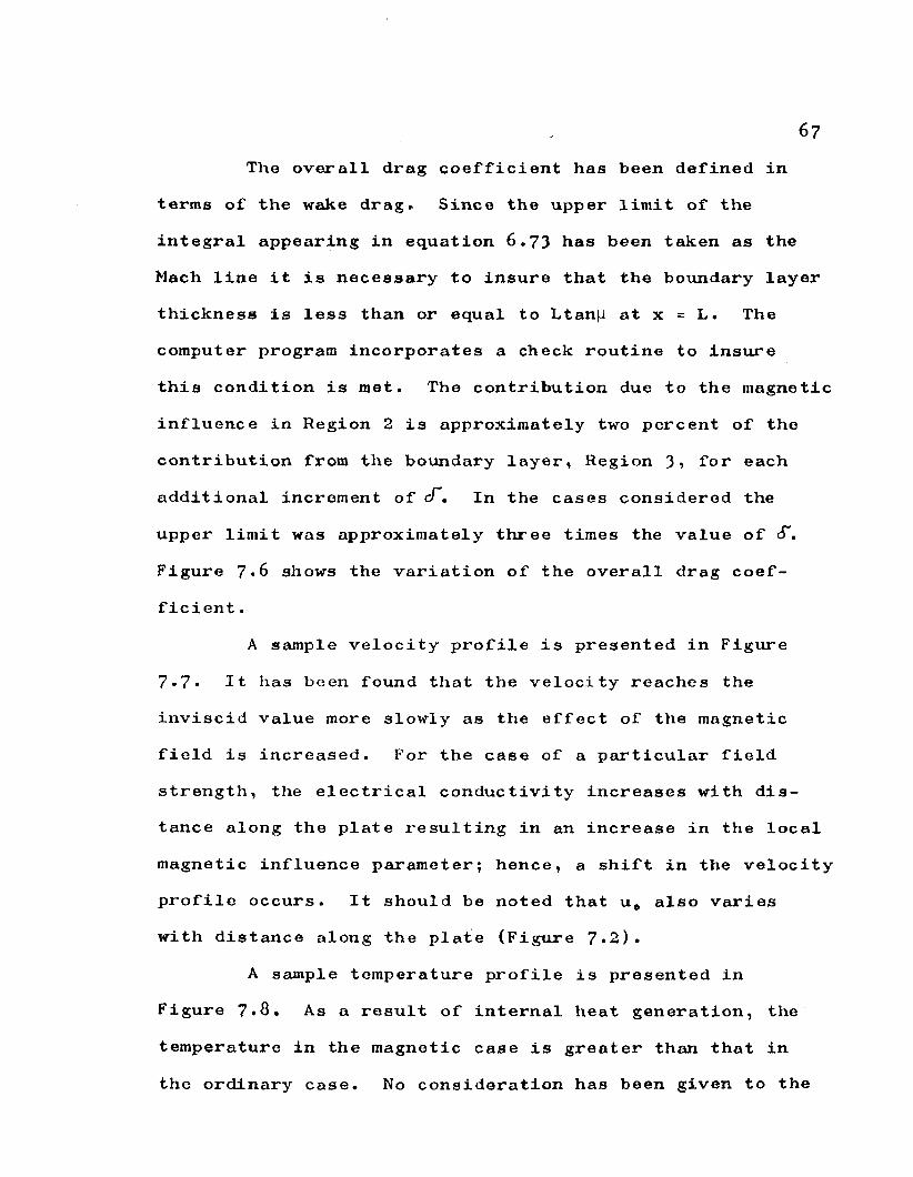
A sample velocity profile is presented in Figure
7«7» It has been found that the velocity reaches the
inviscid value more slowly as the effect of the magnetic
field is increased. For the case of a particular field
strength, the electrical conductivity increases with dis
tance along the plate resulting in an increase in the local
magnetic influence parameter; hence, a shift in the velocity
profile occurs. It should be noted that ua also varies
with distance along the plate (Figure 7»2).
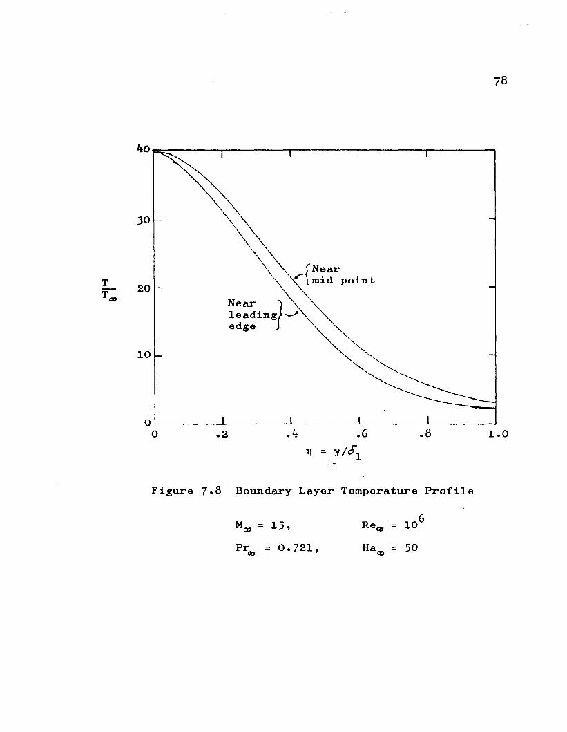
A sample temperature profile is presented in
Figure 7»8« As a result of internal heat generation, the
temperature in the magnetic case is greater than that in
the ordinary case. No consideration has been given to the
Page 78
68 t
fact that the thermal boundary layer thickness and the
momentum boundary layer thickness are different. As was
pointed out in Chapter IV, the thermal boundary layer
thickness can be much larger than the velocity boundary
layer thickness when the Prandtl number is not approxi
mately unity.
The body shape factor, p, is a measure of the
pressure gradient along the plate. Equation 6.9 shovrs
that separation occurs for p = -12. Figure 7«9 shows the
variation of P with distance along the plate for various
Hartmann numbers and = 15• Since it has been assumed
that the applied pressure gradient is zero, for a zero
Hartmann number 3-0. As the Hartmann number increases,
P increases negatively, and for sufficiently high values
of the Hartmann number separation occurs.
Approximate Solutions
Two useful equations can be obtained from the
computer solutions by fitting curves to the data. The
boundary layer growth may be expressed as
{- 2.12(1 J^iM|)'701(Re)U"501(g),750eI
I^8-6ft + 11-0)10
(7.3)
while the location of separation may be expressed as
Re = ^ * = 4.03xl09(Ma,)"1*51(Haa>)~1,113 (7 - ) H'Cb
Page 79
69
The error resulting from these equations is less than 5% in
the ranges:
.l*x/L*l;
20 ;
O'Ha^ilO3;
k 6 10 i Re. s 3x10 .
Equation 7«3 is not valid once separation occurs. Equation
7*3 overestimates the thickness near the leading edge by a
factor of 10 or more. Equation 7 predicts separation
earlier than the computer solution for the low Mach numbers.
Figures 7.10 and 7«H show the approximate solutions and
the computer solutions for the boundary layer thickness and
the location of the separation point respectively.
Summary
The results of this analysis show that a signifi
cant change in the boundary layer thickness and the total
drag is possible for reasonable values of electrical con
ductivity and magnetic field strength. Also it has been
demonstrated that separation can be induced by the applica
tion of a magnetic field. It should be recalled that this
effect is due to the induced pressure gradient. For large
Mach numbers, all results are more sensitive to variations
in the Hartmann number. Since the magnetic effect is
velocity dependent, the increased effect is reasonable.
Finally, it has been established that the velocity and the
Page 80
70
temperature vary with position along the plate. Hence a
true similarity condition does not exist as in the case of
ordinary flow (Blasius solution). In all cases, the solu
tions reduce to within one percent of those given in
Schlichting (22) find von Karmaln (l4) for ordinary flow.
While no experimental results are available at the present,
the assumptions made indicate results which, when compared
with experimental results, should be within the error
limits of current ordinary boundary layer analysis.
Page 81
71
1.0 M,
10
CD
.k .6 . 8 0 . 2 1 . 0
Figure 7»1 Mach Number Decay in Region 2
Re<D = 106, Pr^ = 0.721
Page 82
72
1.1 «
1.0
1.2
d>
1.0
co
6 .4 . 8 1.0 o . 2 x/L
Figure 7.2 Flow Pareuneters in the Inviscid Region
M, = 15, Prw = 0.721
Re. = 106, Ha<0 = 10
Page 83
73
5
Corresponds to von KeArmsth (l4) solution
0 1 . 0 x/L
1 L_ I I I _l I I I I J 0 105 3xl05 5xl05 7xl05 10
fi u _ x 00 <9
Re = — ®x
Figure 7*3 Boundary Layer Development
Mco = 5, = 106
Pr = 0.721, L = 60 inches CD '
The profile for Ha = 0 is within 1% of that given by von Kefrman for laminar compressible flow (l*») .
Page 84
7 4
6
k
2 Corresponds to von Ka'rmrfn (l4) solution
0 .6 .4 . 8 0 2 1.0
0 105 3xl05 5xl05 7xl05 10
=(^] •*x L H J®
Figure 7»4 Boundary Layer Development
= 15 He. = 106
Pr^, = 0*721 L = 60 inches
The profile for = 0 is within 1% of that given by von Ka'rmefn for laminar compressible flow (l4) .
Page 85
75
1.0
.75
TJ u o
o
25
k 6 . 8 0 . 2 1.0
x/L
, Figure 7.5 Local Skin Friction Coefficient Variation Along the Plate
= 15 = 106
Pr^ » 0.721
Page 86
25 50 75 100
Ha. 00
Figure 7»6 Coefficient of Total Drag for Laminar Flow Region
Pr , = 0.721
L = 60 inches
Page 87
77
1.0
Separation occurs at .87 x/L
8
. 6 Near 50% of plate length,
Near 80% of plate lengt!
Near leading edge of plate
. 2
0 .4 6 8 0 . 2 1.0
u/u#
Figure 7«7 Boundary Layer Velocity Profile
* 15, Re^ = 106
= 50, Pr^ = 0.721
Page 88
78
40
Near mid point
20 Near leading edge J
10
A 6 8 1.0 0 2 *
T1 - y/S1
Figure 7«8 Boundary Layer Temperature Profile
M* = 15, Re«, = 106
Pr^ = 0.721, Ha# = 50
Page 89
79
- 2
P
Flow separates when 3 < -12
-10
-12
. 6 8 0 . 2 1.0
x/L
Figure 7*9 Body Shape Factor
= 15, Re« = 106
Pr^ = 0.721
Page 90
8o
10
o H 1.0 X
* -8
® Computed solution
Approximate solution using the empirical equation 7*3
. 8 1 . 0 .1 • 3 .5 . 2 x/L
Figure 7«10 Approximate Boundary Layer Development
L = 60 inches, Re<® = 10^
Page 91
8l
20 -
10
8 .0
5.0
m
o H 3-0
:2.
<S> Computed points
Approximate solution using the empirical equation
30 50 80 100 200 300 500 800 1000 10 20
05, B|L2 1/2 Ha®' ( *
Figure 7.11 Location of Separation Point
(3 = -12, L = 60 inches
Page 93
APPENDIX A
ENERGY EQUATION ANALYSIS
It has been demonstrated in Chapter VI that for the
case of an adiabatic wall the enthalpy ratio may be ex
pressed as a function of u. If, in a more general case, we
assume the enthalpy can be expressed as
h = a +bu + cu2 (A.l)
the energy equation, with Pr = 1, may be written as
2 3 (b + 2cu) (/>uuy+/Jvuy)+/>(u bx+cxu-' + axu)
= "IS +£rB®u2 + MUy + l'L2c(uy + UUyy)+libUyy + li(bXU + CXu2) U*2)
Multiplying the momentum equation by b +2cu and subtracting
the resulting expression from equation A.2 yields
/>u(ax+bxu + cxu2) = +cr D«u)
+ (2c + l)u(^ + °"B2u)
+ U u ( b +c u) 1 X X
+ ^(2c+l)u2 (A.3) K y
Since equation A.3 must hold at the wall
dP„ o / . v 0 = b-z 1- fj. ( 2c + l) (u ) (A.4)
dx w y w
83
Page 94
Q k
If b / 0, c must be at least a function of x and the wall
shear. Returning to equation A.3 and equating like powers
3 of u, the coefficient of u is
c =0 (A.5) x
which contradicts equation A.k. Also, since the velocity-
gradient varies through the boundary layer, it is not
possible to eliminate the non-linear term appearing in
equation A.3«
2 If the coefficient of u is considered, it is found
that
bx = f(u, Uy, c, cx) (A.6)
which is contrary to the assumption that b and its deriva
tives are not functions of u. Hence it must be concluded
that equation A.l is wrong unless b = 0, which is the
adiabatic wall condition.
If a, b, and c are considered as functions of x and
y, the same contradictions result. This is to be expected
since u is primarily a function of y.
If the velocity gradient is assumed to be a constant
(a fair approximation for hypersonic flow), it is possible
to obtain the following differential equation for the
enthalpy ratio, h* = h/h#,
Page 95
I i H? 9
h* +PrRe-^(l + r|)h* +PrRe ax
= -Pr(tf-1)M^-RePr (A.7)
This equation may be used to replace equations 6.79
and 6.82 in the computer program. It should be noted that
P(x), equation 6.50, is also changed. The resulting pro
gram exceeds 10,000 words which is the word storage on the
available system.
coupled by their derivatives, the following process could
be used to obtain a computer solution.
1. z , .. is calculated for a given x. adiabatic
2. h* and its derivatives are calculated based on the
adiabatic solution.
3» z is again calculated, as is h* based on equation
6.29.
k. A variation in either variable greater than an
acceptable error causes a recycling, otherwise a
new value of x is calculated.
For one set of free stream flow conditions, this analysis
required approximately two hours of computer time to reach
a quarter of the length of the plate (Ax = 0.25). It is
estimated that approximately one hundred hours of computer
time would be necessary to obtain sufficient information
Since the resulting equations for z and h* are
Page 96
86
for valid conclusions. Therefore, the run was discontinued
due to the small amount of additional relevent information
which could be obtained.
Page 97
APPENDIX B
FORTRAN LANGUAGE PROGRAM
The following Fortran Language program was used to
obtain the solution of the set of equations for the
adiabatic flat plate* As it is presented here, each equa
tion number denotes one Fortran statement as it would
appear when the standard card format is used. In a few
cases the statement length exceeds the field length per
mitted for cards. In practice, such statements are placed
on two or more cards. However, for the purpose of clarity,
the statement is written as if it could be placed on one
card. Data cards would follow the program in the case of
an actual computer run. All data cards use a floating
point format. The first data card is the number of sets of
free stream data. The number begins in column 7« The
following card or cards are the free stream conditions for
a particular problem. Each card has the following format:
the Mach number, beginning in column 115 the Hartmann
number, beginning in column 21; the Reynolds number,
beginning in column 315 the ratio of specific heats,
beginning in column kl; the Prandtl number, beginning in
column 51and the length of the plate in inches, beginning
in column 6l. The time required to complete the analysis
Page 98
88
for one set of free stream conditions is approximately five
minutes exclusive of the time required for compiling and
printing.
1 FORMAT (10X, 6F10.0) (B.l
2 FORMAT(30H FLOW GOES SUBSONIC AT X = 1PE20.8)(B.2
k FORMAT (1H0 16X,1I1X l8x,4HBETA 13X,10HL0CAL MACH 13X,5HDELTA) (B.3
5 FORMAT (1110 3X,1P4E20.7) (B.4
6 FORMAT (1111 8H MI = (1PE13.4), 8H MPI = (1PE13.Z»)) (B.5
7 FORMAT (9H TI = 1PE13.4), 8H RE = (1PE13.4)) (B.6
8 FORMAT (1H0 l6X, 1HX 17X, 5HTHETA l4X,llHDRAG COEFF. 8X, 10HSKIN FRICT ) (B.7
9 FORMAT (1H0 JX, 1P4E20.7) (B.8
19 FORMAT (3X, 1P4E20.7) (B.9
26 FORMAT (6X, 1F8.0) (B.IO
60 FORMAT (9X, 8HF0R X = 1PE20.7, 11X, 8HFOR X = 1PE20.7) (B.ll
61 FORMAT (10X, 3IIETA 187, 4IIU/U0 22X,3META 19X, 4IIU/U0) (B.12
62 FORMAT (3X, 1P2E20.7 > 5X, 1P2E20.7) (B.13
127 FORMAT(16X,1HX16X,6IIU0/U0016X,6HT0/T0016X, 6HP0/P00l6X,6HD0/D00) (B.lk
128 FORMAT (IHO 3X, 1P5E20.7) (B.15
140 FORMAT (IHO) (B.l6
209 FORMAT (32H INCORRECT DATA FORMAT CARD ) (B.17
215 FORMAT (38H ORDER OF PRINT OUT AB1,AB,XL1, XL,EB ) (B.18
Page 99
89
216 FORMAT (3X, 1P5E20.7) (B.19)
521 FORMAT (4X, 3HETA 17X, 1III1 19X, 1HII 19X, IIHi 19X, 1HII ) (D . 20)
522 FORMAT (3X, F6.3, 1P4E20.7) (B.21)
523 FORMAT (3X, 9HF0R X = 4E20.7) (B.22)
DIMENSION U0I(105), T0I(105), PII(105), R0I(105) (B.23)
DIMENSION BEI(105),DELI(105),FMAJ(105),XI(105) (B.2*t)
DIMENSION THEI(105), CFl(l05) (B.25)
DIMENSION DUDI(105), UUl(l05,ll), ETl(ll) (B.26)
DIMENSION F0C2(k), FLC(4), TC(4), Ql(4), Pl(4) (B.27)
DIMENSION A k ( k ) , FHl(l05,ll) (B.28)
QI = 4.8 (B.29)
BK = 0.1380 (B.30)
TINF = 530. (B.31)
DX = 0.001 (B.32)
E = 2.718282 (B.33)
AK = 0.0 (B.34)
READ 26, AJ (B.35)
30 READ 1, FMAI, FHA, RE, G, FLE, PR (B.36)
FL = FILA*FHA/RE (B.37)
FMI = 12.'FL/FLE (B.38)
PR = PR/2. (B.39)
C INVISCID MACH NO. DECAY TIIRU STM 207 (B.^O)
IF (FL) 208,206,205 (B.4l)
208 PRINT 6,FMAI,FL (B.^2)
PRINT 7, TINF, RE (B.^3)
Page 100
90
PRINT 209 (B.44)
GO TO 403 (B.45)
206 EB = 0.0 (B. 46)
GO TO 207 (B.47)
205 AB1 = (1. +(G-l.)*FMAI* FMAI/2.)/(1.+G-1)*0.32* FMAI*FMAI) (B.48)
AB = 0.64*(AB1**((G+1.)/(G-1.))) (B.49)
XL1 = LOGEF(AB) (B.50)
XL = XL1/(2.0*G*FL*FMAI*FMAI) (B.51)
EB = -XL1/(FL*XL) (B.52)
IF(EB) 207,212,212 (B.53)
212 PRINT 6, FMAI, FL (B.54)
PRINT 7, TINF, RE (B.55)
PRINT 215 (B.56)
PRINT 216, AB1,AB,XL1,XL,EB (B.57)
GO TO 403 (B.58)
207 AK = AK +1.0 (B.59)
64 DUDY = 1.0 (B.60)
UO = 1.0 (B.61)
TO = 1.0 (B.62)
PI = 1.0 (B.63)
RO = 1.0 (B.64)
65 UUO = 1.0 (B.65)
X = 0.0 (B.66)
THE - 0.0 (B.67)
CFX =0.0 (B.68)
Page 101
91
BE = 0.0 (B.69)
DEL = 0.0 (B.70)
10 GH = (G-1.0)/2. (B.71)
FMI2 = FMAI*FMAI (B.72)
GM = GH*FMI2 (B.73)
ST = SQRTF(TI) ' (B.74)
FO = l./FMAI (B.75)
FMU - FO +(F0* * 3)/6. + 3 . *(FO* * 5)/40. +5.* (FO* * 7)/128. (B.76)
Z1 = 0.0 (B.77)
II = 1 (B.78)
1 = 1 ( B . 7 9 )
DO 300 J = 1,1001 (B.80)
FMAO = FMAI*E* *(EB*FL*X) (B.8l)
IF(FMA0-1.>11,11,12 (B.82)
11 GO TO 399 (B.83)
12 IF(11-j) 13,14,15 (B.84)
13 GO TO 403 (B.85)
14 FMAJ(I) = FMAO (B.86)
UOI(I) = UO (B.87)
TOI(I) = TO (B.88)
PII(I ) = PI (B.89)
ROI(I) = RO (B.90)
BEI(I) = BE (B.91)
DELI(I) - DEL *FLE (B.92)
XI(I) = X (B.93)
Page 102
92
67 DUDI(I) = DUDY ( B . 9*t)
THEI(I) = THE*FLE (B.95)
CFI(I) = CFX (B.96)
VELOCITY PROFILE (B.97)
92 ET = 0.0 (B.98)
93 DO 100 L = 1,11 (B.99)
95 FBE = 2.0* ET -2.0 *(ET * * 3) +ET**4 (B.100)
96 GBE = (ET -3•0*(ET* * 2) +3.0*(ET**3) -ET* * k) /(> .0 (B.101)
97 UUI(I,L) = FBE + BE*GBE (B.102)
ETI(L) = ET (B.103)
98 ET = ET + 0.1 ( B . l O k )
100 CONTINUE (B.105)
INVISCID FLOW THRU 71+2 (B.106)
15 FMAO = FMAI*E* *(EB*FL*X) (B.107)
FMA2 = FMAO ""FMAO (B.IOS)
FM = FMI* FMI2/FMA2 (B.109)
GMO = FMA 2 * GH (B.110)
68 El = E**(2.0*EB*FL*X) (B.lll)
EB1 = G*FMI2/(2.*EB) (B.112)
E2 = E**(G*(G-1.)*FMI2*FL*X) (B.113)
U02 = (FMI2 -1. )/(FMI2*El -1.) (B.ll*t)
U01 = U02* *EB1 (B.115)
UO = E2*U01 (B.116)
IF(UO)399,70,71 (B.117)
71 TO = E2/(U0**(G-1.0)) (B.118)
Page 103
93
PI = TO/UO (B.119)
RO = I.O/UO (B.120)
DELTA ITERATION THROUGH STMT 99 (B.121)
•70 FK = -G*FL*FMI2/(FMA2-1.0) + FL*FMI2/FMA2 (B.122)
FKP = -G*FL*GMI2/(FMA2-1.) (B.123)
43 AA = 37./315. -BE/9^5• -BE«BE/90?2. (B.12^)
B = 8113./4O45. -97•'BE/90090.0 -379.*BE*BE /2162160.0 -BE*BE*BE/6l7760. (B.125)
Q = (12.+BE)•(12.+BE)/2160.0 (B.126)
Gl = (2. -(B -PR * Q) /AA ) * Gil (B.127)
G2 = (2. -(B-Q)/AA)*GH (B.128) I
G4 = (1.3 +19 • *BE/120 . -19. *(.2. +BE/6 . ) /20•)*AA (B.129)
T = TO* (FM*G4t+ (l. +FMA2*Gl)/(l. +FMA2*G2)) (B.130)
IONIZATION PERCENT (B.131)
XA = 0•001*SQRTF(E * *(-QI/(BK*TINF))*TINF •*1.25 (B.132)
XB - (E**(QI*(l.-TO)/(BK*TINF))*(TO**2.5) (B.133)
FI = SQRTF(XB/(XA *XA * PI +XB)) *0.001 (B.134)
FMO - TO *(1.-FI) +T0* *(5•/2. ) *FI (B.135)
222 REI.= RE*UO*RO/FMO (B.136)
PRI= PR*FM0/2. (B.137)
IF(ABSF(REI-RE) -0.02)220,220,221 (B.I38)
221 RE = REI (B.139)
PR = PRI (B.1^0)
GO TO 70 (B.l4l)
220 CONTINUE (B.l42)
Page 104
94
Fl = 1.0 +BE/12. (B.143)
F2 = 215•*BE*BE/9072• -871.*BE/756O. -33./70. (B.l44)
F3 = -AA (B.145)
F4 = 83./630. -79.•BE/7560. -BE»BE/4536. (B.I46)
F5 = 1. +BE/120. (B.147)
69 RAT = U0*Fl*T/2.0 (B.148)
16 CHI = X (B.149)
DO 17 N = 1,3 (B.150)
FOC = FMAI*E*•(EB*FL*CHl) (B.151)
F0C2(N) = FOC *FOC (B.152)
FLC(N) = FL*FMI2/F0C2(N) (B.153)
TC(N) = TO*(FMI*FMI2*G4/FOC2(N) +(l. +F0C2 (N)*G1)/(1. +FOC 2 ( N )*G2)) (B.154)
17 CHI = C1II + DX/2. (B.155)
DO 18 NN = 1,3 (B.156)
Ql(NN) = Fl/(AA'RE) (B.157)
PO a ((0.7+BE/120.)/(2.•AA) -(2.-F0C2(NN)) /2.)* F KP (B.158)
PP = (FL*FMI2*(.6-19^*TC(NN)*TC(NN)/20.) /F0C2(NN)-FK*(.6+.4*TC(NN)))/(2.*AA) (B.159)
18 Pl(NN) = PO +PP (B.160)
A1 = DX*(Q1(l)+P1(1)*Z1) (B.l6l)
A2 = DX*(Q1(2)+P1(2)*(Zl+Al/2.)) (B.l62)
A3 = DX*(Q1(3)+P1(3)*(Zl+2.*A2 -Al)) (B.I63)
Z2 = Z1 + (Al + 4.*A2 + A3)/6 (B.164)
IF(Z2)20,21,21 (B.165)
20 DI = ABSF(Z2) (B.l66)
Page 105
95
DIN = SQRTF(DI) (B.167)
PRINT6, FMAI,FMI (B.168)
PRINT 7, TINF, RE (B.I69)
PRINT19, BE, X, FMAO, DIN (B.170)
GO TO 54 (B.171)
21 DEL = SQRTF(Z2) (B.172)
89 IF(DEL -0.0)90,90,91 (B.173)
90 DUDY = 9.8765 (B.174)
GO TO 99 (B.175)
91 DUDY = RAT/DEL (B.176)
99 BE = T*RE*Z2*FK (B.177)
THE = AA*DEL (B.178)
LEADING EDGE VARIATION (B.179)
601 IF(J-1)403,201,202 (B.180)
201 X = X +0.0001 (B.181)
IF(X-0.001) 15,700,700 (B.182)
202 X = X +0.001 (B.183)
o
o
1 ^-
CONTINUE (B.184)
DRAG COEFF (B.185)
120 DET = 0.0 (B.186)
DCD = 0.0 (B.187)
CDM =0.0 (B.188)
DO 125 IJ = 1,11 (B.189)
FBI = 2.* DET-2.*(DET * * 3) +DET**4 (B.190)
GBI = (DET -3•*(DET* *2) +3.*(DET*•3) -DET**4)/6. (B.191)
UUJ = FBI +BE*GBI (B.192)
Page 106
96
DCD = DEL*DET*UO»UUJ*(l.-UO'UUJ) (B.193)
CDM = CDM +DCD (B.194)
125 DET = DET +0.1 (B.195)
YD = X*(FMU+(FMU **3)/3*+2.*(FMU * * 5 )/l5•+17•* (FMU*•7)/315•) (B.I96)
DY = YD -DEL (B.197)
IF(DY)104,105,105 (B.198)
104 CFX = CDM (B.199)
GO TO 106 (B.200)
105 CFX a CDM +DYM1.-U0) (B.201)
106 CONTINUE (B.202)
Z1 - Z2 (B.203)
C TEMP PROFILE THRU STM 520 (B.204)
C STM 511 IS ADIABATIC WALL CONDITION (B.205)
IF(11-J ) 403,510,520 (B.206)
510 FII = T (B.207)
511 FHP = 0.0 (B.208)
ET = 1.0 (B.209)
DET = 0.01 (B.210)
FII = FI (B.211)
IT = 1 (B.212)
IK = 1 (B.213)
DO 500 IJ a 1,101 (B.214)
503 IF(IK-IJ) 403,504,505 (B.215)
504 FHI(I,IT) = FH'FMO (B.216)
IK = IK +10 (B.217)
Page 107
97
IT = IT +1 (B.218)
505 CONTINUE (B.219)
ET = ET -DET (B.220)
703 CONTINUE (B.221)
FBE = 2.0* ET -2.0 *(ET * * 3) +ET**4 (B.222)
GBE = (ET -3.0*(ET**2) +3«0*(ET**3) -ET**4)/6.0 (B.223)
U = FBE + BE*GBE (B.224)
FII = 1. +FMA2*(PR* *0.5)*GII*(1.-U) (B.225)
IONIZATION PERCENT (B.226)
XA = XB (B.227)
XB = (E* *(QI* (1. -FII) /(BK*TO*TINF)*(FII* *2.5) (B.228)
FI = SQRT(XB/(XA*XA*PI +XB) *0.001 (B.229)
FMO = FII* (1. -FI) +FH**(5./2. ) *FI (B.230)
REI = RE*U0/(FMO * FII) (B.231)
PRI= PR*FM0/2 (B.232)
IF( ABSF(PRI-PR) -0.02) 701,701,702 (U.233)
702 PR = PRI (B.234)
RE = REI (B.235)
GO TO 703 (B.236)
701 CONTINUE (B.237)
500 CONTINUE (B.238)
II = II +10 (B.239)
I = 1+1 (B.240)
520 CONTINUE (B.2kl)
C = ABSF(BE) (B.2k2)
Page 108
98
IF(C-12.)300,300,399 (B.2^3)
300 CONTINUE (B.244)
399 PRINT6, FMAI,FMI (B.245)
PRINT 7, TINF, RE (B.246)
IF(FMAO-1.) 53,53,5^ (B.247)
53 PRINT 2, X (B.248)
5^ M = II (B.2^9)
IF(M-6O) 51,51,52 (B.250)
51 N = 1 (B.251)
GO TO 400 (B.252)
52 N = 5 (B.253)
C X, BETA, MO, B. L. THICKNESS PRINT OUT (B.254)
400 PRINT4 (B.255)
PRINT5, (XI(K),BEI(K),FMAJ(K),DELI(K), K = 1,I,N) (B.256)
PRINT 140 (B.257)
C INVISCID FLOW PRINT OUT (B.258)
PRINT 140 (B.259)
PRINT 127 (B.260)
PRINT 128,(XI(K),U0I(K),TOI(K),PIl(K), ROI(K),K=1,I,N) (B.261)
C X, THETA, DRAG, SKIN FRICT, PRINT OUT (B.262)
PRINT 140 (B.263)
PRINT 8 (B.264)
PRINT 9, (XI(K),THEI(K), CFI(K), DUDI(K), K = 1,1,N) (B.265)
C MODIFIED VELOCITY PROFILE PRINT OUT (B.266)
Page 109
99
PRINT 140 (B.267)
101 PRINT 60, XI(1), XI(26) (D.268)
PRINT 6l (B.269)
PRINT 62,(ETI(L),UUI(1,L),ETI(L),UUI(26,L), L =1,11) (B.270)
IF(l-5l)52zt,102,102 (B.271)
102 PRINT 140 (B.272)
PRINT 60, XI(51), XI(76) (B.273)
PRINT 6l (B.274)
PRINT 62,(ETI(L), UUI(51,L), ETI(L), UUI(76,L), L = 1,11) (B.275)
IF(I-100)52^,103,103 (B.276)
103 PRINT l40 (B.277)
PRINT 60, XI(100), XI(IOI) (B.278)
PRINT 6l (B.279)
PRINT 62,(ETI(L), UUl(lOO,L), ETI(L), UUI(101,L) , L=l,ll) (B.280)
524 CONTINUE (B.281)
C MODIFIED TEMP PROFILE PRINT OUT (B.282)
PRINT l40 (B.283)
PRINT523, XI(1), XI(26), XI(76), XI(lOl) (B.284)
PRINT l40 (B.285)
PRINT 521 (B.286)
PRINT 522, (ETI(L), FHI(1,L), FHI(26,L), FHI(76,L), FHI(101,L), L = 1,11) (B.287)
404 IF(AJ-AK)403,403,30 (B.288)
403 STOP (B.289)
END (B.290)
Page 110
SYMBOLS
a Speed of sound
B Magnetic flux density
cd Coefficient of total drag
cf Coefficient of viscous drag (skin friction)
c P
Specific heat at constant pressure
D Displacement vector
E Defined by equation 4.29
E Electric intensity
exp Natural exponential
f(Tl) Velocity ratio (see equation 6.1)
F (n) Component of f ()
G(ri) Component of f ( r|)
h Enthalpy
H Magnetic intensity
Ha Hartmann number, (CB^L^/y.)^"^^
"i?T Unit vectors
J Electrical current
k Boltzman's constant (Chapter II)
k Coefficient of thermal conductivity
K Component of P, defined by equation 6 .44
f K Component of (3, defined by equation 6 .44
L Length
100
Page 111
101
In Natural logarithm
M Mach number
P Pressure
Pr Prandtl number, ^c^/k
P(x) Defined by equation 6.6l
q Velocity vector
Q(x) Defined by equation 6.62
r Larmor radius e
R Gas constant
Re Reynolds number, />uL/[J.
t Time
T Temperature (Chapter II)
T Density ratio at the wall (Chapter VI)
u,v Components of velocity
x,y Coordinates
z ^/L2
P Body shape factor, defined by equation 6.8
if Ratio of Specific heats
cT Boundary layer thickness
^ Momentum boundary layer thickness
Defined by equation 6.26
4 Defined by equation 6.27
Permittivity
T\ Dimensionless coordinate, defined by equation 6.1
Q Defined by equation 6.25
Defined by equation G.JO
Page 112
e<r Defined by equation 6.31
X 2 Magnetic influence parameter, CrB h/jiu
A Coefficient of thermal conductivity (Chapter II)
Coefficient of viscosity
lJe Permeability
^1 Second coefficient of viscosity
Tt Constant, 3-1^1592 . . .
Density
o - Electrical conductivity
f w
Wall shear
£ Dissipation function, defined by equation 3» 11
Defined by equation 4.26
Superscripts
( )* Dimensionless quantity
I ( ) First derivative with respect to independent
variable (exception is K defined above)
Subscripts
( )# Inviscid flow variable
( Free stream flow variable
Operators
4—, — Partial derivatives dx ay
4—, 4— Total derivatives dxT dy
Page 113
103
k - k + « - v < >
* - * %
Variables appearing in only one section are defined when
used.
Page 114
REFERENCES
1. Bertram, M. H., "An Approximate Method for Determining the Displacement Effects and Viscous Drag of Laminar Boundary Layers in Two-Dimensional Hypersonic Flow," NACA, T.N. 2773, 1952.
2. Bogdonoff, S. M. and A. G. Hammitt, "Fluid Dynamic Effects at Speeds from M 11 to 15i" of the Aero. Sci., V23, #2, pl08, 1956.
3« Braum, Willis II., "Stagnation Boundary Layer with Arbitrary Pressure Gradient," NASA, TND-1703, 1963.
4. Chapman, S., "The Viscosity and Thermal Conductivity of a Completely Ionized Gas," Astrophys. J., V120, #1, pl51, 195^.
5. Engel, A. von, Ionized Gases, Oxford Univ. Press, London, 1955*
6. Gilmore, F. R., "Equilibrium Composition and Thermodynamic Properties of Air to 24,000 K," Project RAND, The Rand Corp., RM-15^3, 1955-
7. Buganov, D. and I. Poshkarev, "Free Spiraling in Magnetic Fields," Soviet Physics, V7, #6, p48o, 1962.
8. Hartmann, J., "Ilg-Dynamics I, Theory of the Laminar Flow of an Electrically Conducting Liquid in a Homogeneous Magnetic Field," Det Kgl. Danske Videnskabernes Selskab., V15, #6, pi, 1937.
9. Hartmann, J. and F. Lazarus, "Hg-Dynamics II, Experimental Investigations on the Flow of Mercury in a Homogeneous Magnetic Field," Pet Kgl. Danske Videnskabernes Selskab., V15, #7, pi, 1937.
10. Hildebrand, Francis B., Advanced Calculus for Applications, Prentice-IIall, Englewood Cliffs, New Jersey, 19&3•
11. Hilsenrath, J. and M. Klein, "Tables of Thermodynamic Properties of Air in Chemical Equilibrium," AEDC, TDR-63-161, 1963.
104
Page 115
105
12. Kaeppeler, H. J. and G. Baumann, "Irreversible Stochastic Thermodynamics and the Transport Phenomena in a Reacting Plasma,1' Mitteilungen aus dem Forschungsinstitut fur Physik der Strahlantriebe E. V«, #8, Stuttgart, 1956•
13» Kantrowitz, A. R. and H. E. Petschek, "An introductory Discussion of Magnetohydrodynamics," Landshoff, R. K., Magnetohydrodynamics, Stanford Univ. Press, Stanford, California, pi, 1957•
lk. Karman, Theodore von and II. S. Tsien, "Boundary Layer in Compressible Fluids," Collected Works of Theodore von Karman, III, 1933-39? Butterworth Scientific Pub., London, 1956.
15. Karman, Theodore von, From Low Speed Aerodynamics to Astronautics, Pergamon Press, New York, 19o3*
16. Lin, S. C., E. L. Resler, and A. Kantrowitz, "Electrical Conductivity of Highly Ionized Argon Produced by Shock Waves," J. of App. Physics, V26, #1, p95, 1955.
17. Lock, R. C., "Stability of the Flow of an Electrically Conducting Fluid Between Parallel Planes Under a Transverse Magnetic Field," Proc. Roy. Soc. A, V233i #1192, P105, 1955-
18. Lysen, J. C. and G. K. Serovy, "The Boundary Layer in a Pressure Gradient," Iowa State University Bulletin, Report No. 4 3» Ames, Iowa, 196%.
19« Moore, L. L., "A Solution of the Laminar Boundary Layer Equations for a Compressible Fluid with Variable Properties, Including Dissociation," J. of the Aero. Sci., V19, #8, P505, 1952.
20. Rossow, Vernon J., "On Flow of Electrically Conducting Fluids over a Flat Plate in the Presence of a Transverse Magnetic Field," NACA, TN #3971, 1957*
21. Saha, M. N., "Ionization in the Solar Chromosphere," Phil. Mag, and J. of Sci., V40, S6, p472, 1920.
22. Schlichting, Herman, Boundary Layer Theory, McGraw-Hill, New York, i960.
Page 116
106
23• Spitzer, L. Jr. and R. Harm, "Transport Phenomena in a completely Ionized Gas," Phya. Rev., V89, #5, P977, 1953-
2k, Stuart, J. T., "On the Stability of Viscous Flow Between Parallel Planes in the Presence of a Coplanar Magnetic Field," Proc. Roy. Soc. A, V221, #1145, pl89, 195^.
25. Truitt, Robert W., Hypersonic Aerodynamics, Ronald Press, New York, 1959«
26. Ts ien, H. S., "Superaerodynamics, Mechanics of Rarefied Gases," J. of the Aero. Sci., V13, #12, p653, 19^6.
27* Williamson, R. R., "On the Equations of State of Ionized Hydrogen," Astrophysical J., V103, #3i pl39» 1946 .