University of Dundee Adaptive time-stepping for incompressible flow part I: scalar advection-diffusion Gresho, Philip M.; Silvester, David J.; Griffiths, David Published in: SIAM Journal on Scientific Computing DOI: 10.1137/070688018 Publication date: 2008 Link to publication in Discovery Research Portal Citation for published version (APA): Gresho, P. M., Silvester, D. J., & Griffiths, D. (2008). Adaptive time-stepping for incompressible flow part I: scalar advection-diffusion. SIAM Journal on Scientific Computing, 30(4), 2018-2054. 10.1137/070688018 General rights Copyright and moral rights for the publications made accessible in Discovery Research Portal are retained by the authors and/or other copyright owners and it is a condition of accessing publications that users recognise and abide by the legal requirements associated with these rights. • Users may download and print one copy of any publication from Discovery Research Portal for the purpose of private study or research. • You may not further distribute the material or use it for any profit-making activity or commercial gain. • You may freely distribute the URL identifying the publication in the public portal. Take down policy If you believe that this document breaches copyright please contact us providing details, and we will remove access to the work immediately and investigate your claim. Download date: 19. Mar. 2016
Transcript
University of Dundee
Adaptive time-stepping for incompressible flow part I: scalar advection-diffusion
Gresho, Philip M.; Silvester, David J.; Griffiths, David
Published in:SIAM Journal on Scientific Computing
DOI:10.1137/070688018
Publication date:2008
Link to publication in Discovery Research Portal
Citation for published version (APA):Gresho, P. M., Silvester, D. J., & Griffiths, D. (2008). Adaptive time-stepping for incompressible flow part I: scalaradvection-diffusion. SIAM Journal on Scientific Computing, 30(4), 2018-2054. 10.1137/070688018
General rightsCopyright and moral rights for the publications made accessible in Discovery Research Portal are retained by the authors and/or othercopyright owners and it is a condition of accessing publications that users recognise and abide by the legal requirements associated withthese rights.
• Users may download and print one copy of any publication from Discovery Research Portal for the purpose of private study or research. • You may not further distribute the material or use it for any profit-making activity or commercial gain. • You may freely distribute the URL identifying the publication in the public portal.
Take down policyIf you believe that this document breaches copyright please contact us providing details, and we will remove access to the work immediatelyand investigate your claim.
SIAM J. SCI. COMPUT. c! 2008 Society for Industrial and Applied MathematicsVol. 30, No. 4, pp. 2018–2054
ADAPTIVE TIME-STEPPING FOR INCOMPRESSIBLE FLOWPART I: SCALAR ADVECTION-DIFFUSION"
PHILIP M. GRESHO† , DAVID F. GRIFFITHS‡ , AND DAVID J. SILVESTER§
Abstract. Even the simplest advection-di!usion problems can exhibit multiple time scales.This means that robust variable step time integrators are a prerequisite if such problems are tobe e"ciently solved computationally. The performance of the second order trapezoid rule usingan explicit Adams–Bashforth method for error control is assessed in this work. This combination isparticularly well suited to long time integration of advection-dominated problems. Herein it is shownthat a stabilized implementation of the trapezoid rule leads to a very e!ective integrator in othersituations: specifically di!usion problems with rough initial data; and general advection-di!usionproblems with di!erent physical time scales governing the system evolution.
1. Background and context. The adaptive time-stepping algorithm that is thefocus of this work is certainly not new. We consider the simplest Adams–Bashforth–Moulton pair. A version of our algorithm is hard-wired as the MATLAB functionode23t, see [24], and the underlying methodology is discussed in any many textbookson the numerical solution of ODEs. See, for example, Henrici [13, p. 258] whereestimation of the truncation error is discussed, or Iserles [16, p. 78], where step-doubling and halving is described.
The aim of this work is to assess the performance of this integrator in the contextof method-of-lines discretization of PDEs that arise in incompressible flow modelling.In particular, we hope to provide insight into the role of adaptive time-stepping inthe context of modelling multiple physical timescales. For this purpose it su!ces torestrict our attention to the following simple model of scalar advection-di"usion:
(1.1)!u
!t+ a
!u
!x! "
!2u
!x2= 0 on 0 " x " 1,
together with the initial condition u(x, 0) = u0(x), and boundary conditions (BCs)
u(0, t) = uL and either,(1.2)
u(1, t) = uR or!u
!x(1, t) = 0,(1.3)
where a # 0 (the advecting velocity), " # 0 (di"usivity), and uL and uR are givenconstants. In part II, we build on the foundation laid in this paper and consider thepotential of the integrator in the context of solving the Navier–Stokes equations.
!Received by the editors April 11, 2007; accepted for publication (in revised form) September7, 2007; published electronically May 14, 2008. This collaboration was supported by EPSRC grantGR/R26092/1.
http://www.siam.org/journals/sisc/30-4/68801.html†Livermore, CA, USA ([email protected]).‡Mathematics Division, University of Dundee, DD1 4HN, Scotland, UK ([email protected].
ac.uk).§School of Mathematics, University of Manchester, M13 9PL, UK ([email protected]).
Spatial discretization will, throughout this paper, be carried out using the stan-dard Galerkin approximation with piecewise linear finite elements on an N -elementmesh. This leads to the system of coupled ODEs
(1.4) M u + Au = f ; u(0) = u0,
where the vector f arises from the BC’s (and is zero in the homogeneous case) and,for a Dirichlet BC at x = 1, u(t) := (U1(t), U2(t), . . . UN#1(t))T , where {Uj} are thenodal values of the finite element approximation. With a Neumann BC at x = 1 thevector u(t) will contain N components. Thus, for a uniform subdivision of intervalsof length h = 1/N , the jth component of (1.4) is the second order centered finitedi"erence equation
(1.5)1
6
!Uj#1 + 4Uj + Uj+1
"+
a
2h[Uj+1 ! Uj#1] !
"
h2[Uj#1 ! 2Uj + Uj+1] = 0.
For further details, see, e.g., Gresho and Sani [7, p. 40]. The matrix A in (1.4)is the sum of a symmetric positive-definite di"usion matrix K and a skew symmetricconvection matrix C, so as to properly mimic their continuous (operator) counterparts.M is the mass matrix associated with a discrete L2 projection operator.
The adaptive time-stepping algorithm that is applied to the ODE system (1.4)is a refined version of the “smart integrator” advocated by Gresho and Sani [7, sec-tion 2.7.3–4]. Our algorithm has three ingredients: time integration, the time stepselection method, and stabilization of the integrator. We discuss each of these sepa-rately below.
Time integration. According to the trapezoid rule (TR), given a vector un $u(tn) and a time step #tn, we compute un+1 $ u(tn +#tn) by solving the implicitsystem
(1.6) un+1 = un + 12#tn(un+1 + un) = un + M#1
#f ! 1
2A(un+1 + un)$.
We advocate TR because it is the most accurate A-stable method commensurate witha second order spatial discretization, and also because it is nondissipative (some con-sideration is given to other linear multistep methods in section 6). This is importantwhen solving advection-dominated problems. Another positive feature is that the lo-cal truncation error is easily estimated by repeating the time step using an explicitsecond order Adams–Bashforth method (AB2):
(1.7) u"n+1 = un +#tnun +
1
2#t2n
%un ! un#1
#tn#1
&.
A more subtle issue is that implemention of this linear multistep pair within aself-adaptive algorithm needs to be done carefully. Indeed, a naive implementationmay well have a tendency to “stall” since rounding errors often accumulate and causethe time steps to asymptote and prevent them from increasing as they should. Thisis illustrated in Figure 1.1 (top) which shows the behavior of #tn versus tn for theinitial value problem (IVP) y = !0.01y, y(0) = 1 with the error per step tolerance(to be defined later) # = 10#4 (%) and # = 10#7 (&). (The first two time stepsare #t0 = #t1 = 10#10.) Instead of increasing to infinity with n, it is found that#tn ' 135.1 in the first case and #tn ' 0.1351 in the second, indicating thatasymptotically,1 #tn ( O(#). The fact that this long-time behavior is spurious is
1This can be proven, but we do not include the proof here.
Fig. 1.1. Top: Log-log of the time steps #tn vs. t for a naive TR-AB2 integration of y = !0.01ywith tolerances ! = 10"4 ("), 10"7 (#), and #t0 = 10"10. Bottom: Corresponding plot using anumerically stable TR-AB2 integrator.
confirmed in Figure 1.1 (bottom) which shows the time step histories obtained fora mathematically equivalent algorithm [14] (see also [7, p. 273]), which uses exactlythe same startup time steps and tolerances. In this case, it is seen that #tn ' ) asn ' ).
Conscious of the need to minimize potential round-o" instability, our implemen-tation of the TR-AB2 pair explicitly computes the vector updates scaled by the timestep to avoid underflow and inhibit subtractive cancellation. Specifically, given un,un, and un, we compute a vector vn via
(1.8)#M + 1
2#tnA$vn = M un !Aun + f ,
and update the TR solution vector and time derivative via
(1.9) un+1 = un + 12#tnvn; un+1 = vn ! un.
(The more obvious way of writing the right-hand side (RHS) of (1.8) as !2Aun + 2fis more prone to the ringing phenomenon discussed later in this section. The reasonfor this is discussed in [7, pp. 272–273].) Similarly, the scaled AB2 update wn isexplicitly given by
and generates the AB2 estimate and the second time derivative (needed for the fol-lowing AB2 step) via
(1.11) u"n+1 = un +#tnwn, un+1 =
un+1 ! un
#tn.
Standard manipulations, see, e.g., [7, p. 265], then lead to the truncation error esti-mate
(1.12) un ! u(tn) =1
12#t3n
...u(t) $ dn =
#tn3(1 +#tn#1/#tn)
%1
2vn ! wn
&.
Time step selection. To control the time integration it is usual to place a user-specified tolerance, #, on the norm of dn+1:
(1.13) *dn+1* " #*u*$.
For our target problem (1.4) we use the L2 function norm
(1.14) *dn* = (dTnMdn)1/2
as this will ensure that #tn remains constant for pure advection. An appropriatechoice for *u*$ is (a possibly user-specified estimate of) the maximum norm of theODE solution over the prescribed time interval.2 Assuming that our ODE system hassmooth third derivatives in time (so that the TR time integration is indeed secondorder accurate) standard manipulation of Taylor series shows that the ratio of succes-sive truncation errors is proportional to the cube of the ratio of successive time steps.This implies that
*dn*(#tn+1/#tn)3 ! #*u*$.
Thus, assuming *u*$ = 1 and invoking equality (corresponding to taking the max-imum possible time step to satisfy the accuracy tolerance at the next step) leads tothe following time step selection heuristic:
(1.15) #tn+1 = #tn (#/*dn*)13 .
To implement this methodology in a practical code there are two start-up issuesthat need to be addressed:
1. AB2 is not self-starting. We suggest computing u0 = M#1(Au0 ! f) andu1 from (1.8) and (1.9) in order to start AB2 at the second timestep. Errorcontrol and #t variation is then switched on at the third time step (#t1 =#t0).
2. Choice of initial time step #t0. Several strategies are available with which tostart the TR method. If an estimate of the initial response time ($0 = 1/|%|,where % is the dominant eigenvalue of the matrix M#1A) is available, thena reasonable choice would be #t0 = 0.01$0#
13 . Alternatively, one may simply
select a conservatively small value for #t0 (say 10#10). With such a choicewe will have rapid growth in the time step: typically dn = O(eps) for thefirst few time steps, where eps is machine precision3 and so #tn+1/#tn =
2$u$# = $u0$ = 1 in all of the examples discussed in this paper.3eps % 2.22 " 10"16 in MATLAB, which is used for all of the examples discussed in this paper.
O((#/eps)1/3) $ 104 when # = 10#4. This rapid growth implies that, forsmall values of n,
tn =n#1'
j=0
#tj $ #tn#1,
and with very few such steps (typically 2–4), a time step is obtained that iscommensurate with $0. This also explains the linear growth of #t with t inFigure 1.1 for both implementations starting from #t0 = 10#10. We discussthe other features of Figure 1.1 in the next section.
A general ODE code (like ode23t) will have many additional heuristics, bells, andwhistles; see, Gresho and Sani [7, p. 275], Hairer, Norsett, and Wanner [12, p. 167],Hundsdorfer and Verwer [15, p. 197] or Shampine, Gladwell, and Thompson [24, p. 27].Our code has just one.
1. Time step rejection. If *dn* > 1.1#, then we consider the local error to betoo large. The step is rejected, the current value of #tn is multiplied by(#/*dn*)1/3, and the step is repeated with this smaller value of #tn.
This “trip” is not really needed when solving advection-di"usion problems: in the runsreported later, rejected steps are extremely rare. The heuristic would be important,however, if the linear algebra solve in the computation of the TR update is done“inexactly” (in particular, using a preconditioned Krylov subspace solver instead ofMATLAB’s sparse solver). This will be the case when applying our adaptive time-stepping methodology to the Navier–Stokes equations, and we, thus, defer furtherdiscussion of rejected steps until part II which will build on the strategy outlined byGresho and Sani [8, section 3.16.4].
Stabilization of the integrator. The solution of the IVP y = !%y, y(0) = y0
solved using the numerically stable TR-AB2 method (as in Figure 1.1 (bottom)) canbe shown to satisfy a recurrence with an explicit solution given by
(1.16)
(yn
1! yn
)=
y0 + 12#t0y0
1 ! 12%#t0
n#1*
j=0
1 ! 12%#tj
1 + 12%#tj
(1
!1
).
Looking at (1.16) suggests a potential problem caused by the product of rationalfactors. As %#tn ' ) the factors for large n tend to !1 and so both yn and 1
! ynwould behave asymptotically like (!1)n—this is the familiar “ringing” phenomenonfor TR. Although we have not observed this problematic behavior when solving scalarODEs, ringing e"ects are often observed for very sti" PDEs (typically with very smallspatial grid sizes to resolve fine detail) with relatively large tolerances on the timestep or towards the end of a simulation when close to steady state. Situations such asthese are discussed by Osterby [22] along with a variety of means of suppressing theoscillations. Our code implements an alternative strategy—time step averaging. Theaveraging is invoked periodically every n" steps. For such a step, having computedthe TR update vn via (1.8) we set tn+1 = tn + 1
2#tn and update the solution vectorsvia the sequence
un = 12 (un + un#1); un = 1
2 (un + un#1);(1.17)
un+1 = un + 14#tnvn; un+1 = 1
2vn.(1.18)
We then compute the next time step using (1.15) and continue the integration.
Fig. 1.2. Left: Log-log plot of #t vs. t for advection-di!usion of a step profile on a Shishkin grid:standard TR-AB2 integrator (#) and stabilized TR-AB2 integrator (") with tolerance ! = 10"3.Right: Corresponding plot for finer tolerance ! = 10"4 .
The averaging process annihilates any contribution of the form (!1)n to thesolution and its time derivative, thus cutting short the “ringing” while maintainingsecond order accuracy. In our code the parameter n" is computed automatically. Wespecify a target time, t", that is longer than the response time $0 = 1/|%|, and thenset n" to be the number of steps taken to reach this time starting from t = 0.4 Thebenefit of this simple stabilization strategy is illustrated in Figure 1.2 which shows thebehavior of stabilized and unstabilized TR-AB2 for advection-di"usion of a step profilewith di"usion parameter " = 10#3 and a Shishkin grid with N = 128 subintervals.More details of the experimental set-up are given in Example 5.2, discussed later.All time steps apart from the first two (both 10#10) are shown. For both the fine(right plot) and coarse (left plot) tolerance the time steps generated by stabilizedand unstabilized versions are very similar up to t $ 10#2. Thereafter the time stepsused by the unstabilized version are smaller (in the coarse case, considerably smaller).Reducing the tolerance in the unstabilized version delays the onset of instability. Thestabilized method for # = 10#4 (in this case with n" = 12) reaches the target timein 43 rather than 249 time steps. For # = 10#3 the frequency of averaging is n" = 9steps and 32 steps are used (as opposed to the 4600 steps required by the unstabilizedversion). It may appear that the averaging process is invoked very frequently butin these experiments it is only called on three times. A more typical value of n"with smaller tolerances is n" $ 100. The ringing e"ect is a consequence of the lackof L-stability in the TR scheme, see [11, p. 45], and is e"ectively countered by ourstabilization process.
An outline of the rest of the paper is as follows. We analyze the behavior ofthe TR-AB2 integrator when applied to a scalar ODE model in the next section.Then, in order to demonstrate the performance of the integrator over a wide rangeof conditions, we discuss six example problems in detail; two pure di"usion problems,three advection-di"usion problems (all advection-dominated), and one pure advectionproblem. In each case we give a (mainly) qualitative analysis explaining the observedbehavior of the integrator. We believe that, at the end, the reader will be stronglyconvinced not only that advection-di"usion problems benefit significantly by the useof an adaptive time integrator but also that studying the behavior of the time stepoften helps to delineate di"erent phases of the evolution.
4t! = 10"4 in all of the examples discussed in this paper.
2. A model ODE problem. To whet the appetite, let us take a closer look atthe performance of a numerically stable version of TR-AB2 (as in Figure 1.1) appliedto the standard scalar ODE test equation
(2.1) y = !%y, y(0) = 1,
with the solution y(t) = e#!t. The general case of % = 1/$ +i& is considered here. Inparticular, $ represents a decay time constant mimicking di"usion and the frequency& gives a simple model for advection. From (1.16) we have yn+1 = (1! 1
2%#tn)/(1 +12%#tn)yn and yn = !%yn, and on substituting into the scalar analogue of (1.12) weget the explicit expression
dn = ! %3#t3nyn12(1 ! 1
2%#tn#1)(1 + 12%#tn)
.
The time step selection heuristic (1.15) then implies that
(2.2) #t3n+1 =12#
|%3yn||%
1 ! 1
2%#tn#1)(1 +
1
2%#tn
&|,
and we deduce that
(2.3)#tn+2
#tn+1=
++++1 + 1
2%#tn+1
1 ! 12%#tn#1
++++1/3
.
This is a three-step recurrence with initial conditions #t0,#t1 prescribed and #t2given by (2.2). To make progress we distinguish the special case +% = 0 from themore general case +% = 1/$ > 0.
First, the recurrence (2.3) is stable and clearly has a constant solution when% = i& (& > 0). From (2.2) we find that
(2.4) #t2 = #t3 = · · · = #tn =(12#)1/3
&+ O(#/&).
Since |yn| = 1, there is no amplitude error—just phase error—and the global error|y(tn) ! yn| ranges between 0 and 2, that is from perfectly in-phase to completelyout-of-phase. This periodic behavior can be further analyzed by setting yn = ei"!ttn ,where &!t = & ! 1
12&3#t2 + O(#t4) is the numerical frequency, so that
|y(tn) ! yn| =++e#i"tn ! e#i"!ttn
++ = 2| sin 12 (& ! &!t)tn|
= 2| sin 124&
3#t2tn| + O(#t4).(2.5)
Thus, provided the time interval [0, t"] is such that &3t"#t2 , 1, the global error issecond order and grows linearly in time (this is typical behavior; see [3, ch. 9], forinstance). This is also illustrated quite clearly in Figure 2.1 (top) where log-log plotsof the global error are shown for tolerances # = 10#4, 10#7 (the errors for t = t1, t2 arenot shown since they are much too small). Using (2.5) leads to the simple estimate,T , of the period of the “beats” in the global error
T = 24'/&3#t2.
For & = 1 and # = 10#4, we get #t $ (12#)1/3 = 0.1063 . . . giving T = 6676.9vis-a-vis the numerical result 6675.6 in Figure 2.1 (bottom).
Second, if #tn+1 # #tn#1 and +% > 0, the RHS of (2.3) is > 1 and so #tn+2 >#tn+1. Thus, by induction, the sequence {#tn} grows monotonically. We will identifythree distinct phases of time step growth in the case +% > 0.
Fig. 2.1. The global error |y(tn)!yn| vs. t for TR-AB2 integration of y = !iy, with tolerances! = 10"4 (") and ! = 10"7 (#).Top: Log-log, Bottom: Log-linear.
A start-up phase. As discussed earlier, see Figure 1.1, the time step rapidly in-creases from any (conservatively small) initial value to a value that is appropriatefor the physical response time $0 = 1/|%| and the selected tolerance. The observedbehavior of #t vs. t (growing and then flattening) can be predicted analytically, atleast in the case of real % [14].
A transient phase as the solution relaxes to its rest state. Insight into the dynam-ical behavior in this phase can be obtained through a modified equation approach(see [29], [10], [9]). We reparameterize time by a pseudo-time variable s discretizedwith constant step-size #s = (12#)1/3. Since #tn/#s, is an approximation to dt/ds,then (2.2) is a consistent finite di"erence approximation of the ODE
(2.6)dt
ds= |%|#1|y|#1/3.
Using the chain rule dyds = !% dt
dsy, gives
(2.7)dy
ds= !%|%|#1|y|#1/3y.
The numerical solution yn of our time integrator and the time levels tn are approxi-mated by y(sn) and t(sn), the solutions of the coupled system (2.6) and (2.7). Mul-
so that, with respect to this new parameterization, the approach to the stationarypoint y = 0 is cubic rather than exponential. Solving (2.8), the steady state will bereached in the finite “pseudo-time” s" = 3|%|/+%, and since sn = n#s this gives atotal of n" = (1/(12#)1/3)(3|%|/+%) time steps. Note that n" is independent of %when % is real. In practice, if we compare n" with n (the actual number of time stepstaken by our integrator to satisfy |yn| < #), then there is almost perfect agreement.A typical set of results is given in Table 2.1.
Equations (2.6) and (2.8) imply (unsurprisingly) that %t = ! log |y|. The assump-tion that |%|#t , 1 can then be used to simplify (2.2) leading to the estimate
(2.9) #tn $ (12#)1/3e%!tn/3
|%| ,
which predicts that the time step will grow exponentially. These predicted time stepsare shown by dotted curves in the top of Figure 2.2 and again the agreement withcomputed time steps is excellent—the predicted and actual behavior is indistinguish-able to graphical accuracy for t < 250. We also indicate by the three vertical solidlines the times at which the numerical solution passes through |y| = #. The modifiedequation (2.7) cannot be expected to be valid in this neighborhood (or for longertimes). (2.9) coincides with the constant time step in (2.4) when +% = 0.
Computed global errors are shown in the bottom of Figure 2.2 for the three valuesof the tolerance #, and it is seen that the global error is reduced by a factor of 100when # is reduced by a factor 1000 in keeping with a global error of O(#2/3). Thetails in Figure 2.2 oscillate when the solution reaches the level of the tolerance andthus begin when t = O(log(1/#)).
Long term behavior. Our computional experiments have been carried out overunreasonably long time intervals in order to display this behavior clearly. As was men-tioned earlier, (2.3) shows that the time steps grow strictly monotonically when +% >0. The rate of increase is largest when #tn#1 $ 2/+%.5 From (2.9), this occurs when
|yn| $3#
2
%+%|%|
&3
,
that is when |yn| = O(#), so that the transient behavior of the true solution is wellover. After this point, the time steps continue to increase by the ratio on the RHS of(2.3). This ratio tends to unity (and becomes independent of %) as #tn ' ), thus therate of increase in the time step is progessively reduced—as can be observed in bothFigure 1.1 (bottom) and Figure 2.2 (top). Notice that, as well as being independentof %, the long term behavior of the time step is clearly independent of #.
5It is theoretically possible for the denominator on the RHS of (2.3) to vanish, in which caseyn = 0 and the calculation stops. We shall ignore this unlikely possibility.
Fig. 2.2. Top: Log-log of the time steps #tn vs. tn for TR-AB2 integration of y = !(0.01+i)y,with ! = 10"4 ("), 10"7 (#), and 10"10 (+). Bottom: Log-linear plots of the global error against t.
3. The heat equation. We now consider the heat equation, that is the case ofa = 0 in (1.1). Our objective is to relate the temporal variation of the time step tothe smoothness of the initial data. To start with, we assume homogeneous DirichletBCs in (1.2) and (1.3) and suppose that u0(x) has a Fourier sine series
(3.1) u0(x) =$'
j=1
aj sin j'x
that satisfies,$
1 a2j < ) so that it is convergent for u0 - L2(0, 1). When the Fourier
coe!cients decay more quickly than this, specifically,,$
j=1 j2#a2
j < ), for some
( > 0, then we say that u0 - H#0 (0, 1), and we define a norm on this space by
(3.2) |u0|2# =1
2
$'
j=1
j2#a2j .
See Babuska and Strouboulis [2, pp. 113–129] for a more complete discussion of thesespaces and the concept of square integrable fractional derivatives. The solution of theheat equation with this initial data can be expressed as
For later reference we bound the norm of uttt. If we assume that u0 - H#(0, 1)(0 " ( < 6), then, by Parseval’s relation,
*uttt*20 =
1
2"6'12
$'
j=1
a2jj
12e#2$j2%2t
" 1
2"6'12(max
je#2&$j2%2t)
$'
j=1
a2jj
2#j12#2#e#2(1#&)$j2%2t
" 1
2"6'12e#2&$%2t
#max
jj12#2#e#2(1#&)$j2%2t
$ $'
j=1
a2jj
2#
= "6'12e#2&$%2t#max
jj12#2#e#2(1#&)$j2%2t
$|u0|2#(3.4)
for any ) - [0, 1).6 Now, maxj j2'e#(j2 = (*/+)' e#', from elementary calculus,leading to the estimate
*uttt*0 " '6"3
%6 ! (
2(1 ! ))"e'2t
&3##/2
e#&$%2t|u|#.(3.5)
The decay in time in (3.5) is associated with the concept of “parabolic smoothing”
(see, for example, [4], [18], [19]): *uttt*0 " Ct#(3##/2)e#&$%2t for t > 0, C being aconstant depending on ", ), and (. For small times the algebraic decay dominateswhereas decay is governed by the exponential factor (with ) arbitrarily close to, butless than one) in the long run. In the case of very smooth initial data, u0 - H#(0, 1)for ( # 6, the maximum in (3.4) occurs at j = 1 and we obtain
(3.6) *uttt*0 " '6"3e#$%2t|u|#,
an exponential decay with a rate that is dictated by the smallest eigenvalue ("'2) ofthe di"usion operator !"uxx; this is independent of (.
We now turn to the analysis of the semidiscrete approximation of the heat equa-tion with homogeneous Dirichlet BCs (as in (1.4))
(3.7) M u = !Ku,
where M and K are symmetric positive-definite tridiagonal matrices. We supposethat the generalized eigenvalue problem
(3.8) Mv = %Kv
has eigenvalues ordered so that %1 < %2 < · · · < %N#1 and associated eigenvectorsnormalized so that vT
j Mvj = 1. The solution of (3.7) can then be written as
(3.9) u(t) =N#1'
j=1
cje#!jtvj ,
where the coe!cients {cj} are determined from the initial data by cj = vTj Mu(0).
6The introduction of " is purely a technical device—its aim is to give the exponential decay atlarge times by choosing " close to, but less than one. It could be avoided by redoing the analysiswith " = 0 with the proviso that the results are only useful at short times. The exponential phase
can then be handled separately, taking u & a1e"!2t sin#x and the spatial and temporal errors fromthe leading terms in (3.20) and (3.22), respectively.
When the TR-AB2 integator is applied to the system (3.7) there are three distincttime scales in the evolution; two of these are directly related to the eigenvalues %j
and the third to parabolic smoothing. These are discussed in turn below.Fast transient. At early times the variation in the solution is dominated by the
fastest transient in (3.9): u(t) $ cNe#!N!1tvN#1 + slower varying terms. Thus, as inthe scalar case (see (2.9)), we have that
(3.10) #tn+1 $ (12#)1/3
|cN#1|1/3%N#1e!N!1tn/3.
Since the high frequency modes in the numerical solution (3.9) bear no relation tothe corresponding modes in the PDE solution, this phase is spurious; the numericalsolution cannot begin to approximate the true solution unless all of the coe!cientsof high frequency modes are su!ciently small (which occurs if the initial data has ahigh degree of smoothness) or have su!ciently decayed.
Smoothing phase. Given the definition of the temporal truncation error, (1.12),we suppose the existence of a constant C such that the bound *dn* " 1
12C#t3n*uttt*0holds. Combining the time step selection heuristic (1.15) with the bounds (3.5) (with) = 0) and (3.6) then leads to the estimate
(3.11) #tn+1 # 1
C% (12#)1/3
|u|1/3# "'2%
-.
/
02$e%2tn
6##
11##/6if ( " 6
e$%2tn/3 if ( > 6.
The lower bound suggests that the time step grows sublinearly for ( < 6 and growsexponentially for ( > 6.
Relaxation to steady state. As t ' ), the solutions of the heat equation and itsspatial approximation are governed by the low frequency eigenvectors correspondingto the smallest eigenvalues: u(t) $ c1e#!1tv1. Thus, as in the scalar case (see (2.9)),we have that
(3.12) #tn+1 $ (12#)1/3
|a1|1/3"'2e$%
2tn/3.
This asymptotic form is more precise than (3.11) for long times in the case ( > 6.As for the ODE model discussed in section 2 there could be two additional (non-
physical) phases of time step growth: the startup phase as #tn grows from its initialvalue, and the long term behavior which is independent of #.
We now give an example that illustrates that these estimates of the time step canbe realized in actual computations.
Example 3.1. Consider the system (3.7) arising from discretizing ut = uxx on0 < x < 1 with BCs u(0, t) = 1, u(1, t) = 0, and an initial condition given by
(3.13) u0(x) = 1 ! |1 ! 2x|', * > 0.
Note that this is rough initial data for all * > 0. In addition to the obvious dis-continuities in derivatives at x =1/2 when * is not an even integer, there are sin-gularities since the initial condition does not satisfy the higher order compatibilityconditions required by the Dirichlet boundary conditions. When u0 is extended as anodd function to the interval (!1, 1), appropriate for homogeneous Dirichlet boundaryconditions, there is a discontinuity in the second derivative at the origin and so thecoe!cients {aj} cannot decay more quickly that 1/j3. Moreover, in view of the dis-
Fig. 3.1. Top: The observed rate of growth of time steps for Example 3.1 (#) and the ratepredicted by (3.14) (solid). Bottom: Log-log plot of time steps #t vs. t for $ = 1
2 (broken line),
$ = 1 (dot-dashed line) and $ = 5 (solid line). The predicted rates for $ = 12 , 5 are shown by dotted
lines.
continuities in derivatives at x = 12 for * < 2, u0 - Hp#)(!1, 1) for any , > 0, where
p = max{* + 12 ,
52}.
7 Given this level of regularity, the estimate (3.11) predicts thatduring the smoothing phase the time step will be bounded below by
(3.14) #tn+1 # Cts, s = max{7/12, 11/12 ! */6},
where the constant C depends on * and |u0|p#).We take a subdivision of N = 256 equal elements and use a small tolerance
# = 10#10 in order to accurately determine the observed rates of growth—obtainedby computing the slopes of the linear regression lines through the values of log#tnversus log tn for tn - [5 % 10#5, 5 % 10#3]. The resulting exponents s are shown onthe top of Figure 3.1 while on the bottom we show log-log plots of #tn against tn for* = 1
2 , 1, 5. The agreement between theory and practice is excellent.8
7The presence of % is a consequence of using the norm (3.2) on H". It could be removed by usinga (more appropriate) Besov space; see [2].
8In order to get this level of agreement, spatial resolution is not as important as having a smalltolerance; increasing ! to 10"7 leads to quite poor agreement while decreasing the number of elementsto 64 has little e!ect (except when $ = 0, which we interpret as the discontinuous function u0(x) =1 ! |1 ! 2x|sign(1 ! 2x)).
Our second example introduces some other important behavioral characteristicswithout the added complication of advection (which will be included in the nextsection).
Example 3.2. Consider the system (1.4) arising from discretizing ut = "uxx on0 < x < 1 with " = 1, BCs u(0, t) = 1, u(1, t) = 0, and an initial condition given byu0(x) = 1 , 0 " x " 1.
This PDE problem is particularly challenging because of the impossibility of ob-taining a solution of “arbitrary” accuracy for x ' 1 and t . 0, owing to the singularitythere. At early times, 0 < t < 10#2, we compare our numerical solution with the clas-sical error function approximation to the solution
(3.15) uerf(x, t) = erf#(1 ! x)/
/4"t
$.
In particular, using Maple 9.5 c!9 we can show that
2222!3uerf
!t3
22222
=
3 1
0
%!3
!t3erf
%1 ! x/
4"t
&&2
dx ( 945
2048
42"/'
t11/2,
where ( indicates that this is accurate up to exponentially small terms of the form
exp(!1/"t). Then, assuming #t $#12#/**3uerf
*t3 *$1/3
, this leads to the estimate
(3.16) #t(t) ( (12#)1/35
2048
9454
2"/'
61/6
t11/12.
Note that the step function initial data has a regularity estimate u0 - H#(0, 1) for( < 1/2, see [2, p. 126], so the factor t11/12 in the time step growth in (3.16) iscompletely consistent with the bound in (3.11).
For t # 10#2 our numerical solution will be compared with the truncated Fourierseries (FS) solution:10
(3.17) un(x, t) = 1 ! x +n'
j=1
2
j'exp(!j2'2"t) sin j'x.
We turn next to the issue of spatial resolution. A notional definition of thethickness of the growing boundary layer at small times is, from (3.15), given by,(t) :=
/4"t (,(0.01) = 0.02 at the time when (3.15) is replaced by (3.17)). We
combine this with the concept of minimum time of believability, see Gresho and Sani[7, p. 196], which is defined by
$MTB := h2/4".
This is the time at which the boundary layer width has grown from zero to approxi-mately h, the distance to the first node from the boundary i.e., ,($MTB) = h. Clearly,no numerical approximation can be accurate for ,(t) , ,($MTB). For ,(t) > ,($MTB)on the other hand—that is for t > $MTB—believability becomes at least plausible.
For a 256-element uniform mesh, the above remarks are validated by the com-putational results shown in Figure 3.2 where we show both the analytical solution
9Copyright (C) Maplesoft, a division of Waterloo Maple Inc.10For 0 < t < 10"2, $u! uerf$# < 10"12, and we can ensure comparable accuracy at later times
$u! un$# < 10"12 by taking n = '5/#(&t) terms of the FS.
Fig. 3.2. Numerical solutions (broken lines) and exact solution (solid lines) in the four elementsnearest the boundary where the singularity is present. Left: Uniform grid. Right: Geometric grid.
(solid line) and the FE solution (broken lines) at four values of t. In this case wehave $MTB $ 3.8% 10#6, and from the figure we see that the numerical solution doesnot resolve the boundary layer before t $ 10#5. We shall analyze the global errorbehavior in more detail in a moment.
Here, in order to make our numerical solution useful for much smaller times(while still retaining its usefulness for larger times, of course) we now introduce a256-element “smart” (or at least, smarter) mesh. To do this we select—admittedlysomewhat arbitrarily—a small time believability limit of $MTB = 10#8 (nearly 400times smaller than with the uniform mesh) and use the definition of $MTB to generatethe smallest grid size h = hmin on our new mesh (hmin = 2 % 10#4, nearly 20 timessmaller than h for the uniform mesh). The remaining nodal locations come from thegeometric formula
hj = -N#jhmin , j = 1 : N,
with the grid ratio - chosen so that,N
j=1 hj = 1. With N = 256 this gives - $ 1.0177and a largest element at x = 0 with hmax $ 0.0176—88 times larger than hmin . Thesolutions at early times in the four elements closest to the singularity are also shownin Figure 3.2. The numerical solution is (almost) useful by t = $MTB(= 10#8) andthe superiority of this grid is clear.
In Figure 3.3 we show, on a log-log scale, how the time step varies for fourcases, two on the uniform mesh and two on the geometric mesh, all starting with#t0 = 10#10. The first point we wish to emphasize is the tremendously large variationin step sizes—eleven orders of magnitude in the “best” case (geometric mesh with# = 10#7) using about 850 time steps (see Table 3.1). Clearly, there is no fixed-#tintegrator that could even begin to compete with this e!cient use of time steps! Thenext thing to note is the numerical agreement with theory: a thousandfold changein # gives a tenfold change in step size. In each case the time steps adjust from theinitial value #t0 = 10#10 to a more (#-dependent) appropriate value in no more thatfour steps.
We have included in Figure 3.3 three vertical broken lines that delineate themain phases of the evolution. The first occurs at t = $MTB: at earlier times thetime step behaves as given by the fast-transient expression (3.10) (shown by a dottedcurve for # = 10#4—the agreement is much better when # = 10#7). The interval$MTB < t < $1 ($MTB $ 4 % 10#6 for the uniform grid and 10#8 for the geometricgrid while $1 = O(1/%1) $ 1/"'2) covers the smoothing phase when the solution is
Fig. 3.3. Log-log plot of time steps #t vs. t for Example 3.2. Left: Uniform grid. Right:Geometric grid. The grids have N = 256 elements, ! = 10"4 ("), and ! = 10"7 (#). Also, shownon the left are the time steps for the geometric grid (') for comparison.
Table 3.1Total number of steps used by uniform and geometric grids in Example 3.2 for 0 < t * 10.
erf –like and the time step is given by the lower bound in (3.11) with ( = 1/2 (or(3.16)). Comparing with the dotted line which has gradient 11/12, it is seen thatthe exponent given for the time step is sharp. The time steps for the geometricand uniform grids for # = 10#7 (Figure 3.3, left, . and &, respectively) are virtuallyidentical for t > 10#5. The constant $2 in Figure 3.3 is the time when the solutionis within O(#) of the steady state. During the third interval $1 < t < $2, the timestep is governed by (3.12) (shown again by a dotted curve for # = 10#4). In the finalinterval t > $2, the time step is governed by the internal dynamics of the TR-AB2integrator and behaves as in the scalar case. Most notably #t is independent of #and the spatial grid; see the discussion at the end of section 2. It is seen in Table 3.1that increasing the number of elements for a given tolerance has a negligible e"ect onthe number of time steps required to integrate up to t = 10. This suggests that thesolution is well resolved spatially. It is also seen that the use of a geometric grid costsan additional 10%–20% time steps but in return the solution is accurately obtainedfor much smaller times.
We now consider the behavior of the global error. We do this back-to-front: wewill first discuss the computational results before deriving analytic bounds for thespatial and temporal errors consistent with the observed behavior. Figure 3.4 showsthe maximum error as a function of time for both meshes (and two values of #) and for127- and 255-term Fourier series. The results show the e"ectiveness of the combinationof a smart time integrator with a smart mesh—it even beats the Fourier series up untilt $ 10#5. (Of course, a really smart mesh would both move and remove nodes astime progressed, ending with just 3 nodes.) For each of these meshes the behaviorof the error goes through several phases. For the uniform mesh the log-log plot ofthe error shown on the top of Figure 3.4 initially behaves like t#1. Also, when N is
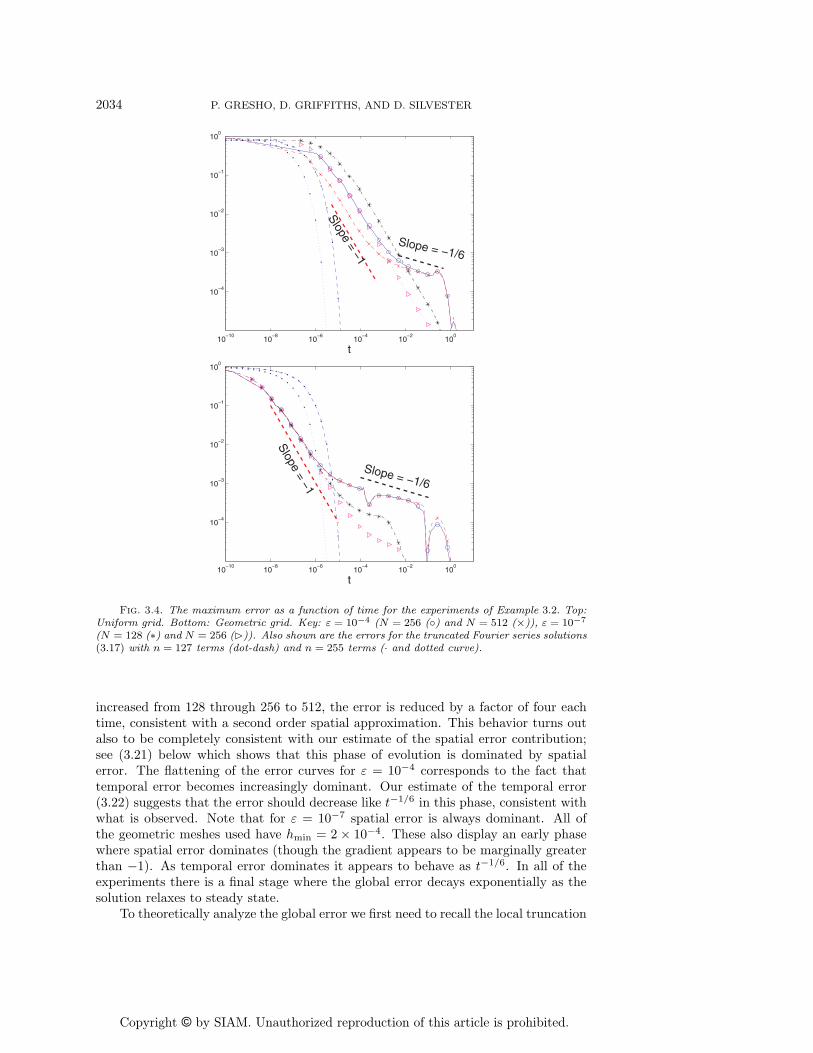
Fig. 3.4. The maximum error as a function of time for the experiments of Example 3.2. Top:Uniform grid. Bottom: Geometric grid. Key: ! = 10"4 (N = 256 (#) and N = 512 (")), ! = 10"7
(N = 128 (+) and N = 256 (!)). Also shown are the errors for the truncated Fourier series solutions(3.17) with n = 127 terms (dot-dash) and n = 255 terms (· and dotted curve).
increased from 128 through 256 to 512, the error is reduced by a factor of four eachtime, consistent with a second order spatial approximation. This behavior turns outalso to be completely consistent with our estimate of the spatial error contribution;see (3.21) below which shows that this phase of evolution is dominated by spatialerror. The flattening of the error curves for # = 10#4 corresponds to the fact thattemporal error becomes increasingly dominant. Our estimate of the temporal error(3.22) suggests that the error should decrease like t#1/6 in this phase, consistent withwhat is observed. Note that for # = 10#7 spatial error is always dominant. All ofthe geometric meshes used have hmin = 2 % 10#4. These also display an early phasewhere spatial error dominates (though the gradient appears to be marginally greaterthan !1). As temporal error dominates it appears to behave as t#1/6. In all of theexperiments there is a final stage where the global error decays exponentially as thesolution relaxes to steady state.
To theoretically analyze the global error we first need to recall the local truncation
error. Specifically, we take the standard uniform grid estimate
(3.18) Tn+1/2j = ! 1
12
("h2 !
4u
!x4+#t2
!3u
!t3
)n+1/2
j
+ . . . ;
see, for example, Morton and Mayers [21, p. 30]. We then take our estimate of theglobal error to be the function e(x, t) that solves the “correction equation”:
(3.19) et = "exx ! 1
12"h2 !
4u
!x4! 1
12#t2
!3u
!t3.
Note that here #t is a function of t.We shall determine bounds on the maximum norms of the spatial and temporal
errors separately, and, to keep things simple (see (3.11)), we assume that ( " 6.(Later we are only really interested in the particular case of ( = 1/2.) With u givenby the Fourier expansion (3.3) the spatial error component, e(S), will be governed by
e(S)t = "e(S)
xx ! 1
12"'4h2
$'
j=1
j4aje#$%2j2t sin j'x
from which we deduce, since e(S)(x, 0) = 0,
(3.20) e(S)(x, t) = ! 1
12"'4h2t
$'
j=1
j4aje#$%2j2t sin j'x,
and hence
*e(S)(·, t)*$ " C"h2t$'
j=1
j4|aj |e#$%2j2t,
where C denotes a generic constant independent of x, t, h,#t. Assuming that u0 -H#(0, 1), we obtain (with any , > 0 and with 0 " ) < 1)
*e(S)(·, t)*$ " Ch2("t)#max
je#&$%2jt
$ $'
j=1
(j#|aj |)j#1/2#)0j9/2##+)e#(1#&)$%2j2t
1
" Ch2("t)e#&$%2t maxj&1
0j9/2##+)e#(1#&)$%2j2t
1 $'
j=1
(j#|aj |)j#1/2#).
Then, since,$
j=1 j#1#2) < ), using the Cauchy–Schwarz inequality gives
(3.21) *e(S)(·, t)*$ " C"h2|u0|#e#&$%2t
("t)5/4##/2#)/2.
For practical purposes, we can set ) = 1 and , = 0. Thus, in the case of interest( = 1/2, our bound suggests that the spatial error initially behaves like t#1 and thenultimately decays exponentially.
The temporal error component e(T ) := e! e(S) is governed by
We now assume that #t(t) is given by the lower bound in (3.11) for ( < 6, that is
e(T )(x, t) = C (#/|u0|#)2/3 ("t)3##/3
$'
j=1
j6aje#$%2j2t sin j'x.
Then, the same argument that was used to estimate the spatial error gives the estimate
(3.22) *e(T )(·, t)*$ " C#2/3|u0|1/3#
e#&$%2t
("t)1/4##/6#)/2.
The algebraic powers of t in (3.22) and (3.21) are equal when ( = 3. For ( < 3 andfor early times the bounds suggest that the spatial error is dominant. In the case ofinterest ( = 1/2, the bound (3.22) is consistent with the behavior seen in Figure 3.4,that is, for dominant temporal error the global error behaves like t#1/6.
In some recent related works, Verfurth [27] has presented a posteriori energy errorestimates of theta time stepping for the fully discretized heat equation, and Akrivis,Makridakis, and Nochetto [1] give refined a posteriori error estimates for TR semidis-cretization of selfadjoint parabolic equations (which does not include convection-di"usion or a discussion of spatial discretization). The nature of corner singularitiesfor the heat equation and their e"ects on numerical simulations have been studied byFlyer and Fornberg [6].
4. Pure advection of a smooth wave form. We now take a rather largestep—from a “rough” di"usion problem to a “smooth” advection problem—in partto see what di"erent aspects of the TR-AB2 might surface. The smoothness of theinitial data assures good spatial resolution with relatively few elements on a uniformgrid. The solution is governed by the ODE system (1.4) with " = 0, and if periodicboundary conditions had been considered, A = C would then be a circulant skew-symmetric matrix. In such a case, as in (3.9), the solution would be written in theform
(4.1) u(t) =N'
j=1
cje#!jtvj ,
except that now %j are imaginary (cf. (2.4)). This would, in turn imply that *u* 0(uTMu)1/2 was conserved in time, as would the time derivatives of the solution: *u*,*u*, and *...u*, which would further imply a constant sequence of time steps
(4.2) #t2 = #t3 = · · · = #tn $ (12#)1/3
*...u*1/3.
Returning to the general (nonperiodic) case, the global error e is defined by thefollowing analogue of (3.19),
Fig. 4.1. Pure advection of Gaussian given by (4.5) at t = 0, 0.25, 0.5.
where T (x, t) is the truncation error term. Since u 0 u(x! at) and #t is constant, itfollows that T 0 T (x! at) and that (4.3) has the solution
(4.4) e(x, t) = t T (x! at),
which implies that the error grows linearly with time along characteristics x ! at =constant. This behavior of the error will also be seen in the following example.
Example 4.1. Consider the system (1.4) arising from discretizing ut + ux = 0 on0 < x " 1, with BC u(0, t) = 0 for t # 0, and the initial condition given by a discreteversion of the Gaussian profile
(4.5) u0(x) = exp{!(x! x0)2/2/2},
which is centered at x0 = 1/2 and which has / = 1//
200 $ 0.071.The semidiscrete equation at x = 1 is given by
(4.6) 16h(2UN + UN#1) + 1
2 (UN ! UN#1) = 0,
which means that K is no longer skew-symmetric. Figure 4.1 shows the numericalsolution at several times for N = 128. Clearly the well-resolved Gaussian is easilytracked through these grids. The TR-AB2 time step histories are shown on the top inFigure 4.2 for two values of N , namely 128 and 256, and two values of the tolerance# = 10#4 and # = 10#7. These time steps can be compared with the “theoreticalvalues” obtained by replacing
...u in (4.2) by !3u$/!t3, where
(4.7) u$(x, t) = exp(!(x! x0 ! t)2/2/2)
is the travelling wave solution that would arise on an infinite span—this prediction isgraphically indistinguishable from the computed values shown up to a time of t $ 5/6,when the Gaussian has e"ectively left the domain. Indeed, for 0 < t ! 0.4 the timestep is constant (to machine precision for # ! 10#5) and may be estimated (in asimilar way to (3.16)) from the full span Gaussian to be
(4.8) #t$ = (12#)1/3#8/5/(15
/')$1/6
,
which gives #t$ $ 9.6% 10#3 for # = 10#4 and is a factor of 10 smaller for # = 10#7,in agreement with Figure 4.2. Also, up to the time t $ 5/6 the time steps di"er im-perceptibly for the two values of N which indicates that the spatial error is negligible.
The global error e = u!U for 0 < t < 0.25 is shown in Figure 4.3 with # = 10#7
and N = 128 and grows according to the predicted form (4.4). The analogous figuresfor the other parameter values scale as #2/3 since the global error is dominated bytemporal error in this time interval.
We return now to the discussion of the time step histories in Figure 4.2. Theexact solution (that is u, not u$) is virtually zero for t > 1 which would lead one to
Fig. 4.2. Time step history for propagation of a Gaussian. Top: Example 4.1, pure advectionon uniform grids with ! = 10"7 and ! = 10"4. Bottom: Example 5.1, advection-di!usion with& = 2 " 10"5 and ! = 10"7.
0
0.2
0.4
0.6
0.8
1
0
0.05
0.1
0.15
0.2
!5
0
5
x 10!5
& xt '
Fig. 4.3. Global error for pure advection of a Gaussian for 0 * t * 0.25, ! = 10"7 and N = 128.
suppose that the time steps should increase to infinity. However, the computed timesteps are approximately constant for 5/6 < t < 11/6. The problem, not apparent onthe scale of Figure 4.1, is that the numerical solution has some di!culty in leaving thecomputational domain cleanly. This is manifested in a very small trail of “wiggles”(with wave lengths $ 2h) that move upstream at the group velocity (!3) of a 2h wave(see Gresho and Sani [7, section 2.6]). The wiggles are a consequence of the outflowequation and their properties can be deduced from the semidiscrete equations. Weanalyze them in some detail since they have a significant bearing on the examples inthe next section.
To isolate the reflections we need to compare the FE solution U with the FEsolution U$ on the domain {(x, t) : !) < x < ), t > 0} with initial data extendedto infinity by zero. However, U$ is an O(h4) approximation to u$, the solution of theadvection equation on the same domain. Since the reflections are of O(h2) it su!cesto look at the truncation error associated with the outflow approximation (4.6) whichgives
TN = h6 (2uN + uN#1) + 1
2 (uN ! uN#1)
= 12h[ut + ux]N ! 1
12h2[2uxt + 3uxx]N + · · · .(4.9)
The reflection induced by T is given by the solution, say -, of the semidiscrete equa-tions (1.5) (with " = 0) with -j(0) = 0 for 0 < j " N , -0(t) = 0 and the outflowequation
(4.10) h6 (2-N + -N#1) + 1
2 (-N ! -N#1) = ! 112h
2u''0(1 ! t),
where the RHS has been obtained by substituting the exact solution u$ = u0(x! t)into the above expression for T . Since the initial data u0 is only defined on the interval(0, 1), the RHS of this equation is nonzero only for 0 < t < 1.
We now assume that the values of - at even and odd numbered grid points areapproximations to separate smooth functions p(x, t) and q(x, t). The internal semidis-crete equations will then be consistent of order O(h2) with the hyperbolic system
To leading order p = q = O(h2) so the first term on the left-hand side (LHS) is O(h3)which may be neglected. This leads to the outflow BC
(4.12) p! q = ! 16h
2u''0(1 ! t)
at x = 1 and the RHS is again zero for t > 1. Adding and subtracting the componentequations in (4.11) reveals that p + q and p! q are constant along the characteristiclines x ! t = constant and x + 3t = constant, respectively (the slopes of these linescorrespond to the group speeds of 1 for long wavelengths and !3 for 2h-wavelengths).
We focus first on the boundary values of the solution. Since p = q = 0 at t = 0and p + q = 0 on the incoming characteristic at x = 1, the BC (4.12) gives
Fig. 4.4. Plots of p and q (scaled by a factor of 100) showing reflections caused by the outflowequation (N = 128) for pure advection (top) and with added di!usion (& = 2"10"5) (bottom). Thehorizontal curves at t = 2/3, 4/3, 7/3 show the numerical error (dots) and predicted behavior (solidlines).
This data is swept into the domain along the left-going characteristic along whichp! q is equal to its value at x = 1. Since p = 0 at x = 0, we then find that
q(0, t) = 16h
2u''0( 4
3 ! t), 13 < t < 4
3
so that the amplitude of q at the left boundary is twice its value at the right boundary.This boundary data is then carried back into the domain along right-going character-istics along which p + q is constant and the process repeats for 4/3 < t < 7/3. (Ourasymptotics break down on this “rebound” because the forcing data on the RHS of(4.12) is zero for t > 1 and higher order terms have to be included.) The computedvalues of U1(t) (corresponding to q(0, t)) and UN#1(t), UN (t) (corresponding to q(1, t)and p(1, t)), for N = 128 and # = 10#7 are shown as vertical curves in Figure 4.4(top). These curves have been amplified by a factor of 100 and the chosen tolerance
is su!ciently small so that spatial errors dominate. The predicted curves are graphi-cally indistinguishable from the computed values. The horizontal curves in Figure 4.4(top) show the computed solutions (dots) at times t = 2
3 ,43 ,
73 (only alternate even
and odd points are shown) and the predicted reflections (solid lines).This explains what is going on in Figure 4.2. The first (left-going) reflection
does not a"ect the growth of #t since *...u* is still dominated by the tail of theexiting Gaussian. The vertical dotted lines in Figure 4.2 are the times the right-going characteristic passing through the peak of the initial profile and its consequentreflections hit the endpoints. Following the reflection from x = 0, the time step isconstant #t = O((#N2)1/3) for 5/6 ! t ! 11/6. At t = 1 with # = 10#7 the ratioof time steps with N = 128 and 256 is 1.598 compared with the predicted ratio of41/3 = 1.587. Subsequent reflections have amplitude O(h4) and so #t = O((#N4)1/3).
5. Advection-di!usion. We are now ready to consider the advection-di"usionequation (1.1) with u(0, t) specified as inflow BC and, as in the previous section,initial data that are smooth on the open interval (0, 1). This precludes, for instance,the study of travelling fronts if they have regions of large gradient. We shall beginwith the easier case of a “natural” outflow BC ux(1, t) = 0 before proceeding to a“hard” BC u(1, t) = 0. The former is perhaps of greatest interest because of thedi!culty in achieving the latter in physical situations, however, the latter has becomea benchmark for computations because of the numerical di!culties it presents.
5.1. Natural outflow boundary conditions. With smooth, compactly sup-ported initial data u0, a weak boundary layer develops gradually at the outflow x = 1.Expanding in the parameter "/a we find that the solution of (1.1) under these condi-tions can be approximated by
(5.1) u(x, t) = u$(x, t) ! "
ae#a(1#x)/$ !u$
!x(x, t),
where the truncation error term is O(("/a)2), and where u$ denotes the correspond-ing infinite span solution with the same initial data extended to be zero outside (0, 1),as in section 4.
If "/a , 1, then the numerical solution is prone to spurious reflections from theright-hand boundary as in the pure advection case discussed above. With the di"usionterm present, the analogues of the hyperbolic system (4.11) and the boundary equation(4.12) are
(5.2)13 (2pt + qt) + aqx = ! 2$
h2 (p! q)13 (pt + 2qt) + apx = 2$
h2 (p! q),
7
and
p! q = TN = 2a ["ux ! 1
12ah2uxx]N + . . . ,
respectively, where TN is the truncation error at the outflow (cf. (4.9)). Followingthe approach in section 4 we substitute the truncated estimate of the solution u(x, t)into the above expression for TN and then solve the system (5.2) with initial datap = q = 0 and boundary datum p = 0 on x = 1. This leads to the conclusion thatp+ q is constant along characteristics x!at = constant, but that there is exponentialdecay,
Fig. 5.1. Global error vs. t for advection-di!usion of a Gaussian.
along left-going characteristics x + 3at = constant.Example 5.1. Consider the system (1.4) arising from discretizing ut+aux = "uxx
on 0 < x " 1, with BCs u(0, t) = 0 and ux(1, t) = 0 for t # 0, and the initial conditiongiven by the Gaussian profile (4.5) as in Example 4.1.
Predicted reflections (solid lines) and the numerical results for a uniform gridwith N = 128 (dots showing alternate even and odd grid values) for the case a = 1," = 2 % 10#5 are also shown in Figure 4.4. Comparing these results with those with" = 0 the level of exponential decay is gentle but noticeable. In order to inhibit thesereflections we clearly require much better resolution of the outflow boundary layer.
Perhaps the simplest way of achieving this increased resolution is to use a so-called Shishkin grid [20, 23]. In such a grid N/2 elements are equally spaced in eachof the subintervals [0, 1 ! +] and [1 ! +, 1], where the “boundary layer thickness” isgiven by,
(5.4) + = min
%1
2,2"
alnN
&.
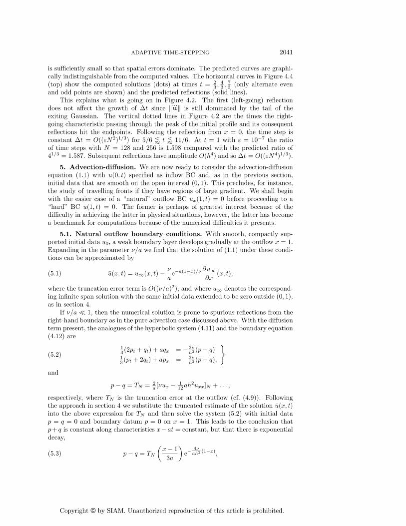
For advection-dominated problems, + = (2"/a) lnN . Using such a Shishkin gridwith N = 256—so that the coarse grid is essentially the same as for the previousexperiment—does not dampen the wiggles for reasons given below. In computationsthe results are graphically indistinguishable from those in Figure 4.4. This can alsobe seen by comparing the second and third rows of Table 5.1 where we give themagnitudes of the reflected waves at x = 1/2, for the times t = 2/3, 4/3, 8/3.
Figure 5.1 shows the behavior of the maximum norm of the global error11 for thecases reported in Table 5.1. In all cases the error is approximately linear in time upto t $ 0.2 (as in (4.4) for pure advection), and grows thereafter up to t $ 0.5 (whenthe peak of the Gaussian meets the right boundary). The error for pure advection isthen nearly constant up to t $ 1.7 except for two peaks near t = 5/6 when the wavereflects from the left boundary, and it finally drops to zero at t $ 2.1. In contrast, forboth the uniform grid (N = 128) and the Shishkin grid (N = 256) when di"usion ispresent, the error decays on 0.5 < t < 5/6 in accordance with (5.3) before mirroringthe behavior seen in the case of pure advection.
Further insight is provided by Figure 5.2 where the computed solution and theglobal errors are plotted for t = 0.4. It can be seen that the uniform grid (N = 128,
11When computing the global error we approximate u(x, t) by the O((&/a)2) approximation (5.1)
which makes use of the infinite span solution u#(x, t) = exp("(x"x0"at)2/(2#2+4$t))(1+2$t/#2
Fig. 5.2. Top: The numerical solution for advection-di!usion of the Gaussian at t = 0.4 with& = 2 " 10"5 for a Shishkin grid (N = 256, dots). Bottom: Global error with a uniform grid(N = 128, circles), Shishkin grid (N = 256, dots), and Geometric grid (N = 256, crosses). Theinterval (1 ! (, 1) has been expanded in order to show the layer solution.
circles) and the Shishkin grid (N = 256, dots) behave in essentially the same mannerfor 0 < x < 1 ! + showing wiggles of roughly equal amplitude. These results suggestthat the reason that the Shishkin grid generates reflected waves is the sharp transitionbetween the coarse and fine grid sizes—such behavior has been known for some timefor pure advection; see, for example [17].
Within the numerical layer (1!+, 1) the magnitude of U = O(a) while the spatialderivatives are well approximated and are of O(a/"). It can then be shown that theanalogue of (5.1) is
for j = N/2 : N . Using this expansion it can be shown that the semidiscrete equationholding at the interface corresponds to the weak implementation of the BC aux = !ut
at x = 1 ! +.To reduce the reflections from the interface we adopt a “smarter” grid that is
defined by
(5.6) hj = 12 (H + h) + 1
2 (H ! h) tanh*( 12 (N + 1) ! j), j = 1 : N
with * = log(5/4), and satisfies h < hj < H, where H and h are, respectively, thecoarse and fine grid sizes used in the Shishkin grid. Since hj approaches its extremevalues geometrically (as j ' ±)), we refer to this as a geometric-Shishkin grid.The largest ratio of consecutive grid sizes for the Shishkin grid is H/h while it ise' = 5/4 for this alternative grid. The grid size sequence {hj} is shown in Figure 5.3
Fig. 5.3. Grid size hj for geometric-Shishkin grid (5.6) for & = 2 " 10"5 and N = 256.
for " = 2% 10#5 and N = 256, when we have + $ 2.2% 10#4 and 111 grid points arelocated in the boundary layer region (1!+, 1). The global error on this geometric gridat t = 0.4 is plotted with crosses in Figure 5.2. It is seen that the amplitude of theerror for x < 1!+ is reduced by a factor of about two, but no wiggles are discernable.The time history of the global error in Figure 5.1 confirms this fact—the plateau isno longer apparent. This better resolution of the physics is also reflected in the timestep behavior using the TR-AB2 integrator. This is illustrated in Figure 4.2. Up untilthe Gaussian meets the right boundary the time step sequence is independent of thegrid used. Thereafter #t is dependent on the amplitude of reflected waves and so itis appreciably larger using the geometric grid compared to the Shishkin and uniformgrids. Although the Shishkin grid solution can be shown to converge uniformly in "as N ' ) [23], our geometric grid is superior (at least for these parameter values).
We have dwelt for some time on the oscillations caused at or near the outflow withthe natural BC employed with the finite element method (FEM). These oscillations areinsignificant when compared with the common finite di"erence treatment of Neumannboundary conditions using the so-called image point method. The superiority of theFEM for natural boundary conditions for advection-di"usion (or Navier–Stokes, forthat matter) is clearly shown by Gresho and Sani [7, p. 209].
5.2. Dirichlet outflow boundary conditions. Our final scenario involvessolving the full advection-di"usion equation (1.1) with smooth initial data u0(x) andboundary conditions u(0, t) = u0(0) and u(1, t) = 0 so that there is a step discontinu-ity at x = 1, t = 0. This scenario is much more challenging than that of the previoussection because here it is the solution u, rather than the flux "ux, that changes by O(1)over the width O("/a) of the layer region. Verhulst [28] provides a brief introductionto singular perturbation techniques for situations such as this.
We consider two example problems. In the first of these we revisit Example 3.2with the addition of advection. The e"ects of advection are confined to the outflowregion and this allows a study of the transition from di"usion-dominated to advection-dominated flow—what we shall refer to as the advection-di"usion time scale ($AD)—inits simplest setting. Our second example then looks at a more complex transition.
Example 5.2. Consider the system (1.4) arising from discretizing ut+aux = "uxx
on 0 < x " 1, with BCs u(0, t) = 1 and u(1, t) = 0, and the step initial conditionu0(x) = 1 , 0 " x < 1.
We take N = 256 and concentrate on the classical Shishkin grid introduced in theprevious section. Such grids are, of course, designed for exponential layers and arenot ideally suited to the narrower erf-like layer that will arise at early times. Resultsobtained for the geometric-Shishkin grid will be discussed subsequently.
Fig. 5.4. Eigenvalues for pure di!usion problem (top) and advection-di!usion (bottom) bothwith & = 10"4 and N = 256. Symbols: Dots (•) correspond to the Shishkin grid and circles (#)correspond to the geometric-Shishkin grid.
For comparison purposes we first discuss the results for the heat equation (a = 0)when using a Shishkin grid with N = 256 that is defined with + = 2" lnN . The sameproblem on a uniform grid was discussed in Example 3.2. The solution of the PDEfor early times is given by (3.15) and relaxes to the steady state u(x, t) = 1 ! x in atime t = O(1/").
The numerical solution, in contrast, evolves in two separate phases. In the firstphase the erf-layer develops entirely within the layer (1!+, 1) and then, in the secondphase, the e"ect of the singularity spreads to the coarse grid on (0, 1 ! +).
An understanding of this evolution requires knowledge of the associated general-ized eigenvalue problem (3.8). The eigenvalues are shown in the top of Figure 5.4.They form two distinct sets, Sc = {%j : j = 1 : N/2! 1}, corresponding to the coarsegrid and Sf = {%j : j = N/2 + 1 : N ! 1} corresponding to the fine grid, with %N/2 a“bridge” between the two sets (its eigenvector has a quite di"erent structure to thosecorresponding to Sc and Sf ). The eigenvalues in these sets are closely approximatedby the eigenvalues of the FE discretization of the di"erential operator !"u'' on thedomains (0, 1 ! +) and (1 ! +, 1), respectively, each with Dirichlet boundary condi-tions (formulae for the discretized operator may be deduced from the results givenin Gresho and Sani [7, p. 190] or [5]). Thus, we have the estimates (confirmed by
that are valid when "N , 1; they show the considerably di"erent time scales onwhich these modes operate. (The estimate for %N/2 is conjectured from the results ofnumerical experimentation.)
Both phases of the numerical evolution have similarities with those in Example 3.2with suitably modified time scales. Each has its own minimum time of believability:
$MTB(h) = h2/4", $MTB(H) = H2/4"
associated with the fine (h) and the coarse (H) grid, respectively. We note that thesetimes are also related to the largest eigenvalues in the sets Sf and Sc: $MTB(h) =O(1/%N#1) and $MTB(H) = O(1/%N/2#1).
After the first four time steps, #t settles into the fast transient mode appropriatefor the fine grid, i.e., #t $ C exp(%N#1t/3) for t < $MTB(h) $ 1.9 % 10#7 (seeFigure 5.5, top, &). The solution then enters the parabolic smoothing phase duringwhich #t increases as t11/12 until t $ $1. At this stage all but the last of the “fastmodes” from Sf have decayed and, for $1 < t < $2, #t $ C exp(%N/2+1t/3) basedon the smallest eigenvalue from Sf . This suggests that $1 = O(1/%N/2+1), where%N/2+1 $ "'2/+2.
An estimate of $2 may be made as the time at which the width of the singular layer(which grows proportional to
/"t) equals the width of the fine grid region:
/"t $ +,
i.e., $2 $ +2/" $ 0.012 so $2 $ 10$1. The e"ect of the singularity subsequentlyspreads into the coarse grid and a second “fast” transient stage begins where #t $C exp(%N/2#1t/3) for $2 < t < $MTB(H) $ 0.15. The solution then enters another
smoothing stage (#t $ Ct11/12) followed by relaxation to steady state (the time stepscorresponding to these later times are not shown as the steady state is not achieveduntil t = O(1/")). Overall, the time step follows the pattern of Figure 3.3 twice insuccession.
In Figure 5.5 we show a linear-log plot of *U ! uerf*$ with time, where uerf isthe solution given by (3.15). (The maximum norm of the di"erence was computedby interpolating uerf onto a finer grid—it is not based on just the nodal errors.)For the heat equation (&) it is seen that the norm decreases and is small ($ 10#2)at t = 10#6—this suggests that the estimate $MTB(h) $ 1.9 % 10#7 is a little toosmall. The norm continues to decrease until t = $1 $ 10#3 when the erf layer beginsto penetrate the coarse grid. During this process, which takes place in the interval$1 < t < $MTB(H), it grows appreciably before decaying again. The norm shows asimilar rise and fall for the geometric-Shishkin grid but it is two orders of magnitudesmaller. The final increase in the norm for t > 103 is due to the fact that uerf doesnot satisfy the boundary condition u(0, t) = 1.
Figure 5.5 also shows a linear-log plot of *U!USS*$with time, where USS = 1!xdenotes the steady state solution of the ODE system when a = 0. The solution iswithin 10#5 of the steady state by t = 104 = O(1/"). Also shown by a broken line isthe maximum di"erence U ! USS computed over only those nodal points lying in thefine Shishkin grid. This shows that the numerical solution becomes close to steadystate relatively quickly in the fine grid (t $ 1).
The main di"erence when using a geometric-Shishkin grid—see Figure 5.5 (top,1 and broken line)—is that #t behaves as Ct11/12 for t > $MTB(h) $ 1.9 % 10#7 and
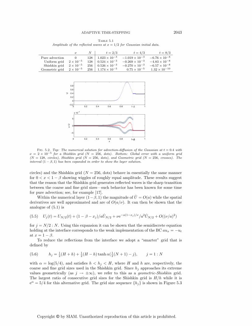
Fig. 5.5. Top: Time step histories for Example 5.2 with & = 10"4, tolerance ! = 10"7, andinitial time step #t0 = 10"10. Bottom: Top: $U ! uerf$# vs. t. Bottom: $U ! USS$# vs. t; thebroken line corresponds to $U !USS$# measured over grid points in (1!(, 1) for the Shishkin grid.Key: Heat equation (a = 0), Shishkin grid (#), heat equation (a = 0), geometric-Shishkin grid (+),AD equation (a = 1), Shishkin grid (!), AD equation (a = 1), and geometric-Shishkin grid (').
does not deviate from this, as the Shishkin grid does, over the interval ($1, $MTB(H)).We attribute this to the fact that the eigenvalues %n (see Figure 5.4, top, shown by&) are more evenly distributed when n is close to N/2.
We now discuss the results of the experiments with advection included (a = 1).At early times the continuum problem is di"usion-dominated; an erf layer forms asdescribed above for the heat equation and the solution is given by u $ uerf(x, t) (cf.(3.15); see, for instance, Flyer and Fornberg [6]). For long times, the solution tendsto the steady state
(5.7) uSS(x) =1 ! e#a(1#x)/$
1 ! e#a/$
having an exponential boundary layer with thickness O("/a). The advection-di"usionequation satisfies a maximum principle so this transition is monotonic.
The eigenvalues of the discrete advection-di"usion operator on a Shishkin gridagain form two distinct sets Sc and Sf ; those in Sc are complex and so it is their modulithat are shown on the bottom of Figure 5.4 (&)—the vertical scale used is the same asthat in the top figure. The larger eigenvalues in Sf are closely approximated by those
of the discrete eigenvalue problem on (1!+, 1) with homogeneous Dirichlet boundaryconditions and are comparable in magnitude with those for the heat equation. Thissuggests that the time scales associated with exponential phases based on the fine gridare also comparable. In particular, the largest eigenvalues are roughly the same sothat $MTB(h) is the same for both problems. The moduli of the eigenvalues in Sc areconsiderably larger than the corresponding eigenvalues of the heat equation thoughthese have little bearing on the solution due to ill conditioning; see Trefethen andEmbree [26].
During the early stages of the evolution, as the erf layer develops, the time stephistory in Figure 5.5 (top, !) is seen to follow that for the heat equation up untiladvection and di"usion have comparable magnitude. This occurs when the widths ofthe erf and exponential layers are comparable:
/"t $ "/a which gives rise to what
we refer to as the advection-di"usion time scale
(5.8) $AD = "/a2
and its location is highlighted in Figure 5.5. This is also the time required for materialto be transported through the width of the exponential boundary layer so is a measureof the time it takes to attain a steady state in the outflow layer. It is clearly aphysical, rather than a numerical time scale—thus correcting the discussion in [7,section 2.6.2g]. The minimum time of believability on the fine grid can be expressedin terms of $AD and N as
(5.9) $MTB(h) =
%2 lnN
N
&2
$AD.
The di"erence *U!uerf*$, shown in Figure 5.5 for a Shishkin grid (!), is a minimumwhen t $ 10#6. The behavior is almost identical for the geometric-Shishkin grid (.).
The next time scale, which is a numerical artifact, occurs when the width of theerf layer (
/"t) grows to that of the fine grid:
/"t = +, leading to $2 = +2/". There
follows a period during which the numerical solution is stationary in the layer and awave emanates to the left with speed !3a and having the same oscillatory structureas that analyzed in section 5.1.
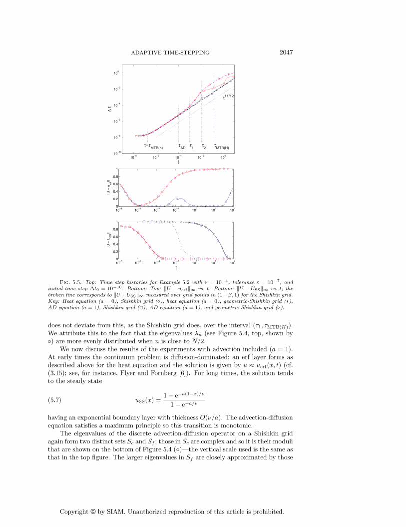
The progress of the solution to steady state is monitored in Figure 5.5 wherewe show *U ! USS*$ as a function of time. It is small when t " 10#3 = 10$AD.The behavior is again almost identical for the geometric-Shishkin grid (.). The nodaldi"erences Uj!uSS(xj) between the numerical and exact solutions (5.7) at steady stateare shown in Figure 5.6 (as a function of j) for Shishkin grid (dots) and geometric-Shishkin grid (solid line) with N = 256. It is seen that the di"erence is oscillatory forthe Shishkin grid when j " N/2 (outside the layer region)12 but the dominant erroroccurs inside the layer region and is of almost identical magnitude for both grids.
When the geometric-Shishkin grid is employed the time step history (see Fig-ure 5.5, top, .) is virtually identical to the classical Shishkin grid while the dynamicsof the solution are restricted to the layer (t < $2). Thereafter, the advection-di"usionsolution evolves using a much larger time step with the geometric-Shishkin grid sincethe amplitude of the 2h–wavelength wave propagating in the negative x-directionfrom the grid interface is much smaller when there is a smooth transition from fine tocoarse grid.
12An explicit expression for the steady state solution on a Shishkin grid is readily obtained fromwhich it can be shown that |UN/2 ! uSS(xN/2)| % 1/N2.
Fig. 5.6. The di!erence between the nodal values of the steady state uSS(xj) of the advection-di!usion equation and the steady state nodal values Uj of the numerical solution on a Shishkin grid(dots) and geometric-Shishkin grid (solid line) for Example 5.2, N = 256, & = 10"4, and a = 1.
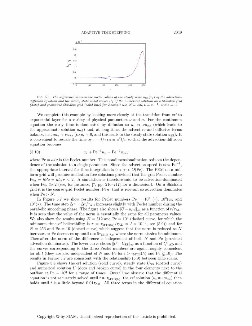
We complete this example by looking more closely at the transition from erf toexponential layer for a variety of physical parameters " and a. For the continuumequation the early time is dominated by di"usion so ut $ "uxx (which leads tothe approximate solution uerf) and, at long time, the advective and di"usive termsbalance, i.e., aux $ "uxx (so ut $ 0, and this leads to the steady state solution uSS). Itis convenient to rescale the time by $ = t/$AD 0 a2t/" so that the advection-di"usionequation becomes
(5.10) u+ + Pe#1ux = Pe#2uxx,
where Pe = a/" is the Peclet number. This nondimensionalization reduces the depen-dence of the solution to a single parameter. Since the advection speed is now Pe#1,the appropriate interval for time integration is 0 < $ < O(Pe). The FEM on a uni-form grid will produce oscillation-free solutions provided that the grid Peclet numberPeh = hPe = ah/" < 2. A simulation is therefore said to be advection-dominatedwhen Peh 2 2 (see, for instance, [7, pp. 216–217] for a discussion). On a Shishkingrid it is the coarse grid Peclet number, PeH , that is relevant so advection dominateswhen Pe > N .
In Figure 5.7 we show results for Peclet numbers Pe = 102 (&), 103(!), and104(1). The time step #$ = #t/$AD increases slightly with Peclet number during theparabolic smoothing phase. The figure also shows *U!uerf*$ as a function of t/$AD.It is seen that the value of the norm is essentially the same for all parameter values.We also show the results using N = 512 and Pe = 103 (dashed curve, for which theminimum time of believability is $ = $MTB(h)/$AD $ 5 % 10#4, see (5.9)) and forN = 256 and Pe = 10 (dotted curve) which suggest that the norm is reduced as Nincreases or Pe decreases up until t $ 5$MTB(h), where the norm attains its minimum.Thereafter the norm of the di"erence is independent of both N and Pe (providedadvection dominates). The lower curve shows *U !USS*$ as a function of t/$AD andthe curves corresponding to the three Peclet numbers are again roughly coincidentfor all t (they are also independent of N and Pe for t > $MTB(h) and Pe " 10). Theresults in Figure 5.7 are consistent with the relationship (5.9) between time scales.
Figure 5.8 shows the erf solution (solid curve), steady state USS (dotted curve)and numerical solution U (dots and broken curve) in the four elements next to theoutflow at Pe = 103 for a range of times. Overall we observe that the di"erentialequation is not accurately solved until t $ $MTB(h); the erf solution (ut $ "uxx) thenholds until t is a little beyond 0.01$AD. All three terms in the di"erential equation
Fig. 5.7. Advection-di!usion problem with step initial data on a geometric-Shishkin grid withN = 256 and ! = 10"7 (Example 5.2) for Pe = 102 (#), Pe = 103 (!), Pe = 104 (+). Top: #) vs.) for the rescaled equation (5.10). Bottom: $U ! uerf$# vs. t/)AD (dotted curve Pe = 10, brokencurve N = 512) and $U ! USS$# vs. t/)AD. The vertical dotted lines are drawn at t = )MTB(h).
have to be retained until steady state (ut $ 0) is approached at $ $ 10. There is nosignificant di"erence for any Peclet numbers Pe # 1.
Our final example incorporates another combination of the time scales seen inExamples 5.1 and 5.2 but with more interesting “physics.”
Example 5.3. Consider the system (1.4) arising from discretizing ut+aux = "uxx
on 0 < x " 1, with BCs u(0, t) = 0 and u(1, t) = 0 for t # 0, and the initial conditionis the Gaussian profile (4.5) centered at the point x = 1 ! / with / = 1/
/200 (see
Figure 5.9).The main di"erences between this and the previous example are that the solution
is nonconstant in the outer region and the amplitude of the outflow boundary layeris also time varying.
With the Dirichlet outflow BC the e"ects of advection are again negligible at earlytimes and the solution is given quite accurately by the approximation (cf. (3.15))
(5.11) u(x, t) $ ue(x, t) 0 u0(x)erf#(1 ! x)/
/4"t
$.
This erf layer then develops into an exponential layer at which stage the solution isgiven, again quite accurately, by the approximation
Fig. 5.8. The erf solution (solid curve), steady state USS (dotted curve), and numerical solutionU of (5.10) (dots and broken curve) in the four elements next to the outflow for Example 5.2 at times) = t/)AD = 1.9 " 10"3(t = )MTB(h)), 10
"2, 10"1, 1, 10 with N = 256, ! = 10"7, and Pe = 103.
0 0.2 0.4 0.6 0.8 10
0.2
0.4
0.6
0.8
1
x
Fig. 5.9. Initial condition for Example 5.3.
where uSS is given by (5.7) and u$ in footnote 11—the latter could equally be replacedby the exact solution for advection on an infinite span: u0(x! at). We shall be moreprecise about the time intervals over which these solutions are valid presently. Thetime-varying Gaussian (the “outer” solution) sets the amplitude of the solution in theboundary layer (the “inner” solution). It is noteworthy that, whereas u$ satisfiesthe full advection-di"usion equation and uSS satisfies the steady state version of thisequation, the solution given by (5.12) satisfies neither—yet does an excellent jobof describing the physics, both within and outwith the boundary layer. A similarstatement applies to (5.11).
The time step histories for the two Shishkin grids are plotted in Figure 5.10.The time step follows the familiar path through the fast transient t ! $MTB(h) then
increases as t11/12 until t $ $AD after which it increases more rapidly as advectiongains in strength. At t = $1, #t reaches the value given by (4.8)—advection isdominant and di"usive e"ects have little influence on its value. At this stage theoutflow boundary layer is fully formed (i.e., is in steady state) with a slowly varyingamplitude, but this variation has little e"ect on #t since the width of the layer is sonarrow that the solution within it makes a negligible contribution to the L2 norm of...U for $1 < t < $2.
Fig. 5.10. Time steps for Example 5.3 on a Shishkin grid (#) and a geometric-Shishkin grid(!) with N = 256, ! = 10"7, a = 1, and & = 10"4.
10!4
10!3
10!2
10!1
100
101
0
0.2
0.4
t = #mtb
||U!u
e|| i
t/#AD
10!4
10!2
100
102
104
0
0.2
0.4
0.6
||U!U
l|| i
t/#AD
t = #mtb
Fig. 5.11. Top: $U ! ue$i, Bottom: $U ! u%$ for the clipped-Gaussian initial data for bothShishkin and geometric-Shishkin grids with N = 256, ! = 10"7 and Pe = 103 (#), Pe = 104 (!),and Pe = 105 (+).
For t > $2 the increase in #t becomes more rapid as the Gaussian “exits” thedomain. Up to this time the two grids generate essentially identical histories. Theconstant $3 in Figure 5.10 is O("/a2). Thus, for t > $3, the numerical solutionsbecome dominated by the spurious reflected waves from the grid interface and thetime steps for the Shishkin grid, having much larger left-going waves, are appreciablysmaller. Also noteworthy is the close similarity of the time step histories for Examples5.2 and 5.3 (except of course for large t).
To estimate the times over which the two solutions, ue and u, (given, respectively,by (5.11) and (5.12)) are valid we compute *U ! ue*$ and *U ! u,*$ and these areshown in Figure 5.11 as functions of $ = t/$AD for Pe = 103 (&), Pe = 104 (!), Pe =105 (1). For fixed N both norms are essentially independent of Peclet number (in theadvection dominated case). Both norms behave quantitatively as in Figure 5.7 whenthe solution in this example is scaled so that the initial amplitude of the discontinuityis unity—the same as for the step data. A detailed study of the solutions in the fourelements closest to the outflow shows a behavior very similar to that in Figure 5.8once the amplitude of the boundary layer solution is taken into account.
A corner singularity can also occur at x = t = 0 caused by the mismatch of theboundary data u(0, t) and u(x, 0) (or their derivatives) as x, t ' 0. The nature of the
singularity is discussed by Flyer and Fornberg [6] and the internal layer created asthe e"ects are propagated into the domain along the characteristic x = at is studiedby Shih [25]. A finite element method with a fixed spatial grid is inappropriate in thecase that a discontinuity occurs since this will generally create oscillatory numericalsolutions. Weaker singularities on the other hand can be handled quite successfullyand the behavior of the time step can be predicted from the level of regularity in thesolution using the techniques described in section 3.
6. Possible extensions. Our examples reveal that even simple problems canhave quite complex time scales, some physical and some of numerical origin, andin this paper we have endeavored, wherever possible, to identify as well as quantifythe di"erent phases of each simulation. It is clear that some form of adaptive timeintegrator is essential in order to e!ciently respond to the di"erent time scales and,given the wide range of dynamics taking place during these simulations, it is ratherreassuring to see the TR-AB2 integrator find the appropriate time step during allphases. We have looked in detail at the way that smoothness of the initial datainfluences the solution, the error, and the selection of time steps. A close study ofthe behavior of the time step can often be useful in shedding light on the di"erenttemporal phases of a simulation.
We note that, of all A-stable linear multistep methods, TR has the smallest errorconstant and therefore allows the largest time step for a given accuracy. For the secondorder backward di"erentiation (BDF) BDF2 method (see Hairer, Norsett, and Wanner[12, p. 401] for the variable step formulation and Hundsdorfer and Verwer [15, p. 203]for numerical results) the error constant is C3 = !2/9 from which we deduce thatthe time step selected by an adaptive time-stepping method will be (3/8)1/3 $ 0.72times smaller than that used by our TR-AB2 method. This has been verified bycomputation; for instance, in Example 3.2, the BDF2 time steps are smaller thanthose shown in Figure 3.3 by the predicted fraction up until t $ $2, after which bothmethods have approximately equal time steps (in keeping with our discussion of longterm behavior in section 2). The same ratio of time steps is observed in pure advectionproblems provided that the tolerance is chosen to be su!ciently small that the timesteps remain essentially constant; otherwise, the dissipative nature of BDF2 causesthe time steps to increase with time.
The theoretical results of this paper have all been based on the principal trunca-tion error term of the TR integrator. For a general pth order linear multistep methodwith error constant Cp+1 (see, for instance, Hairer, Norsett, and Wanner [12]) weobtain, using (1.15),
#tn $%
#
|Cp+1| *u(p+1)*
& 1p+1
.
Thus, for specific model problems, such as the examples used in this paper, it ispossible to compare the e!ciency of methods of di"ering orders as a prelude to theuse of variable step-variable order methods. We intend to pursue these ideas in futurepublications.
Acknowledgments. Thanks are due to John Dold of the University of Manch-ester for improving our understanding of PDE asymptotics, and especially to AlanHindmarsh who has been a guiding light to the “smart” time integration of ODE’s(and DAE’s, when Navier–Stokes is addressed) over the last thirty years; this paperis dedicated to him.
[1] G. Akrivis, C. Makridakis, and R. Nochetto, A posteriori error estimates for the Crank–Nicolson method for parabolic equations, Math. Comp., 75 (2006), pp. 511–531.
[2] I. Babuska and T. Strouboulis, The Finite Element Method and its Reliability, OxfordUniversity Press, New York, 2001.
[3] M. P. Calvo and J. M. Sanz-Serna, Numerical Hamiltonian Problems, Appl. Math. Math.Comput., 7, Chapman & Hall, 1994.
[4] T. F. Dupont, A short survey of parabolic Galerkin methods, in The Mathematical Basis ofFinite Element Methods, Inst. Math. Appl. Conf. New Ser. 2, D. F. Gri"ths, ed., UniversityPress, Oxford, 1984, pp. 27–40.
[5] R. Fletcher and D. F. Griffiths, The generalized eigenvalue problem for certain unsym-metric band matrices, Linear Algebra Appl., 29 (1980), pp. 139–149.
[6] N. Flyer and B. Fornberg, Accurate numerical resolution of transients in initial-boundaryvalue problems for the heat equation, J. Comput. Phys., 184 (2003), pp. 526–539.
[7] P. M. Gresho and R. L. Sani, Incompressible Flow and the Finite Element Method, Vol. 1:Advection-Di!usion, John Wiley & Sons, Chichester, UK, 2000.
[8] P. M. Gresho and R. L. Sani, Incompressible Flow and the Finite Element Method, Vol. 2:Isothermal Laminar Flow, John Wiley & Sons, Chichester, UK, 2000.
[9] D. F. Griffiths, The dynamics of some linear multistep methods with step-size control, inNumerical Analysis 1987, Pitman Res. Notes Math. Ser. 170, D. F. Gri"ths and G. A.Watson, eds., Longman, Harlow, Sci. Tech., UK, 1988, pp. 115–134.
[10] D. F. Griffiths and J. M. Sanz-Serna, On the scope of the method of modified equations,SIAM J. Sci. Statist. Comput., 7 (1986), pp. 994–1008.
[11] E. Hairer and G. Wanner, Solving Ordinary Di!erential Equations, II, Sti! and Di!erential-Algebraic Problems, Springer-Verlag, Berlin, 1991.
[12] E. Hairer, S. P. Norsett, and G. Wanner, Solving Ordinary Di!erential Equations I. Non-sti! Problems, Springer-Verlag, Berlin, 1993.
[13] P. Henrici, Discrete Variable Methods in Ordinary Di!erential Equations, John Wiley & Sons,New York, 1962.
[14] A. C. Hindmarsh, private communication, 2003.[15] W. Hundsdorfer and J. G. Verwer, Numerical Solution of Time-Dependent Advection-
[16] A. Iserles, A First Course in the Numerical Analysis of Di!erential Equations, CambridgeUniversity Press, Cambridge, UK, 1996.
[17] H.-O. Kreiss and J. Oliger, Methods for the approximate solution of time dependent prob-lems, GARP Publications Series 10, World Meteorological Organization, Geneva, 1973.
[18] M. Luskin and R. Rannacher, On the smoothing property of the Crank–Nicolson scheme,Applicable Anal., 14 (1982), pp. 117–135.
[19] M. Luskin and R. Rannacher, On the smoothing property of the Galerkin method for parabolicequations, SIAM J. Numer. Anal., 19 (1982), pp. 93–113.
[20] J. J. H. Miller, E. O’Riordan, and G. I. Shishkin, Fitted Numerical Methods for SingularPerturbation Problems, World Scientific, River Edge, NJ, 1996.
[21] K. W. Morton and D. F. Mayers, Numerical Solution of Partial Di!erential Equations,2nd ed., Cambridge University Press, 2005.
[22] O. Osterby, Five ways of reducing the Crank–Nicolson oscillations, BIT, 43 (2003), pp. 811–822.
[23] H.-G. Roos, M. Stynes, and L. Tobiska, Numerical methods for singularly perturbed dif-ferential equations, in Convection Di!usion and Flow Problems, Springer Ser. Computat.Math. 24, Springer–Verlag, Berlin, 1996.
[24] L. F. Shampine, I. Gladwell, and S. Thompson, Solving ODEs with MATLAB, CambridgeUniversity Press, Cambridge, UK, 2003.
[25] S.-D. Shih, On a class of singularly perturbed parabolic equations, ZAMM Z. Angew. Math.Mech., 81 (2001), pp. 337–345.
[26] L. N. Trefethen and M. Embree, Spectra and Pseudospectra, in The Behavior of NonnormalMatrices and Operators, Princeton University Press, Princeton, NJ, 2005.
[27] R. Verfurth, A posteriori error estimates for finite element discretizations of the heat equa-tion, Calcolo, 40 (2003), pp. 195–212.
[28] F. Verhulst, Methods and Applications of Singular Perturbations: Boundary Layers andMultiple Timescale Dynamics, Texts Appl. Math. 50, Springer, New York, 2005.
[29] R. F. Warming and B. J. Hyett, The modified equation approach to the stability and accuracyanalysis of finite-di!erence methods, J. Comput. Phys., 14 (1974), pp. 159–179.