Unsupervised Learning of Categorical Segments in Image Collections

Unsupervised Learning ofCategorical Segments in Image Collections

Marco Andreetto, Lihi Zelnik-Manor, Member, IEEE, and Pietro Perona

Abstract—Which one comes first: segmentation or recognition? We propose a unified framework for carrying out the two

simultaneously and without supervision. The framework combines a flexible probabilistic model, for representing the shape and

appearance of each segment, with the popular “bag of visual words” model for recognition. If applied to a collection of images, our

framework can simultaneously discover the segments of each image and the correspondence between such segments, without

supervision. Such recurring segments may be thought of as the “parts” of corresponding objects that appear multiple times in the

image collection. Thus, the model may be used for learning new categories, detecting/classifying objects, and segmenting images,

without using expensive human annotation.

Index Terms—Computer vision, image segmentation, unsupervised object recognition, graphical models, density estimation, scene

analysis.

Ç

1 INTRODUCTION

IMAGE segmentation and recognition have long beenassociated in the vision literature. Three views have been

entertained on their relationship: 1) Segmentation is apreprocessing step for recognition: First you divide up theimage into homogeneous regions, then recognition proceedsby classifying and combining these regions [1], [2], [3], [4].2) Segmentation is a by-product of recognition: Once weknow that there is an object in a given position, we mayposit the components of the object and this may helpsegmentation [5], [6]. 3) Segmentation and recognition maybe performed independently; in particular, recognition doesnot require segmentation or grouping [7], [8], [9], [10], [11].These views are not mutually exclusive, while segmentationand recognition are not necessary for each other, bothbenefit from each other. It is therefore intuitive thatrecognition and segmentation might have to be carried outtogether, rather than in sequence, in order to obtain the bestresults. We explore here the idea of carrying out categorylearning for recognition and segmentation jointly—wepropose and study a simple probabilistic model that allowsa unified view of both tasks. Our model represents eachimage as a composition of segments, where a segment couldcorrespond to a whole object (e.g., a cow) or to a part of anobject (e.g., a leg), to a patch of a distinctive texture, or to a

“nonsense” homogeneous region in the background. Theinference process divides each image into segments, anddiscovers segments that are similar across multiple images,thus discovering new visual categories.

We build upon recent work on recognition and segmen-tation. First, we choose to represent image segments usingsimple statistics of “visual words” as features. Using “bagsof visual words” to characterize the appearance of an imagesegment combines an idea coming from the literature ontexture, where Leung and Malik [12] proposed vector-quantizing image patches to produce a small dictionary of“textons,” and an idea from the literature on documentretrieval, where statistics of words are used to classifydocuments [13]. Early visual recognition papers using “bagsof visual words” considered the image as a single bag [14],[15], [11], while recently we have seen efforts either toclassify independently multiple regions per image, afterimage segmentation [3], [4], [16] or to force nearby visualwords to have the same statistics [17]. Recent literature onimage segmentation successfully combines the notion thatimages are “piecewise smooth” with the notion that segmentshapes are more often than not “simple.” These insightshave been pursued with parametric probabilistic models[18], [19], with nonparametric deterministic models [20],hierarchical segmentation models [21], and nonparametricprobabilistic models [22]. The last is a very simple probabil-istic formulation which, as we shall see, combines gracefullywith the popular LDA model for visual recognition.

Our work most closely builds upon two papers: Russellet al. [3] and Andreetto et al. [22]. In the paper of Russell et al.,a “bag of words” representation is used to describe the visualappearance of different segments in images. These segmentsare extracted prior to inference, and are computed indepen-dently of the visual words contained in them. Our workcombines segmentation and category model learning in asingle step, rather than first carrying out segmentation andthen categorizing the segments. While Russell et al.’ssegmentation is independent for each image, in our work

1842 IEEE TRANSACTIONS ON PATTERN ANALYSIS AND MACHINE INTELLIGENCE, VOL. 34, NO. 9, SEPTEMBER 2012

. M. Andreetto is with Google Los Angeles (US-LAX-BIN), 340 MainStreet, Venice, CA 90291. E-mail: [email protected].

. L. Zelnik-Manor is with the Department of Electrical Engineering, TheTechnion-Israel Institute of Technology, Haifa 32000, Israel.E-mail: [email protected].

. P. Perona is with the Department of Electrical Engineering, CaliforniaInstitute of Technology, 1200 East California Blvd., MC 136-93, Pasadena,CA 91125. E-mail: [email protected].

Manuscript received 12 Dec. 2009; revised 23 Nov. 2010; accepted 22 Nov.2011; published online 22 Dec. 2011.Recommended for acceptance by S. Belongie.For information on obtaining reprints of this article, please send e-mail to:[email protected], and reference IEEECS Log NumberTPAMI-2009-12-0814.Digital Object Identifier no. 10.1109/TPAMI.2011.268.

0162-8828/12/$31.00 � 2012 IEEE Published by the IEEE Computer Society

segmentation is carried out simultaneously and eachsegment’s definition benefits from related segments beingsimultaneously discovered in other images. Conversely,Andreetto et al. segment an entire collection of imagessimultaneously, while discovering the correspondence be-tween homologous segments. However, the features thatrelate segments are restricted to size, shape, and averagecolor of the segments. Associating bags of visual words toeach segment enables us to discover more interesting visualconnections between corresponding segments, and thusdiscover visual categories. We develop the simultaneoussegmentation/recognition scheme step by step. We start(Section 2) by proposing a probabilistic model for segmentingindividual images. Then, we further extend the model toincorporate a richer set of visual features (Section 3). Thisprovides a model for automatic inference of categoricalsegments.

2 A PROBABILISTIC MODEL FOR SINGLE IMAGE

SEGMENTATION

Image segmentation techniques may be categorized intothree broad classes. The first class consists of deterministicheuristic methods, such as k-means, mean-shift [24], andagglomerative methods [25]. When the heuristic captures thestatistics of the data, they perform well. For example,k-means provides good results when the data are blob-likeand the agglomerative approach succeeds when clusters aredense and there is little noise. However, these methods oftenfail with more complex data [26].

The second class consists of probabilistic methods thatexplicitly estimate parametric models of the data, such asexpectation maximization for fitting Gaussian mixturemodels (GMM) [27]. The GMM method is principled andcan easily be used as a building block of a larger model thataddresses a more general task. However, when the data arearranged in complex and unknown shapes, as is the case forimages, it tends to fail as, in GMM, each class is representedby a Gaussian (see Fig. 4).

Complex data are handled well by the third class ofmethods, consisting of the many variants of spectralfactorization [28], [26], [20], [29], [30]. These techniques donot make strong assumptions about the shape of clusters

and thus generally perform well on images. Unfortunately,integrating them into larger probabilistic models to tacklemore complex problems, such as recognition and segmen-tation [3] or segmentation with prior knowledge [31], isusually convoluted. We propose a generative probabilisticmodel that can describe segments of complex shape andappearance and can easily be used as a building block for amore complex probabilistic model. Unlike previous prob-abilistic models, it contains a nonparametric componentallowing complex-shaped groups to be modeled faithfully.Unlike factorization methods, it is probabilistic in nature,allowing easy extensions to situations where prior informa-tion is available and integration into larger probabilisticmodels that address more complex problems such asrecognition and motion segmentation [22].

Let x1; x2; . . . ; xN be a set of observations in IRD generatedfromK independent processes fC1; . . . ; CKg. Each processCkis described by a density function fkðxÞ. These densityfunctions are not restricted to any specific parametric family,such as Gaussian densities; we only assume that they aresmooth functions (see Section 2.1.1). The observationsx1; x2; . . . ; xN are generated as follows (see Fig. 1):

1. Select a set of K mixing coefficients �1; �2; . . . ; �K ,drawing them from a probability distribution pð�Þ (seeSection 2.2). Each �k will correspond to a process Ck.

2. For n equal 1 to N :

3. Select one of the K processes Ck by sampling thehidden variable cn according to a multinomialdistribution with parameters �1; �2; . . . ; �K .

4. Draw the observationxn according to the process-specific probability density function fkðxÞ.

Rather than obtaining samples from the model of Fig. 1, weare interested in the inverse problem: computing the poster-ior distribution of the hidden variables cc ¼ fc1; c2; . . . cNggiven the observed variables xx ¼ fx1; x2; . . .xNg. UsingBayes’ theorem we have

pðccjxxÞ / pðxxjccÞpðccÞ; ð1Þ

where the mixing coefficients �k have been marginalizedout from the joint distribution pðcc; �Þ, leaving just the prior

ANDREETTO ET AL.: UNSUPERVISED LEARNING OF CATEGORICAL SEGMENTS IN IMAGE COLLECTIONS 1843

Fig. 1. Left: Plate diagram [23] of our generative model for image segmentation. The gray node xn represents the observations (pixel features). Thenode cn represents the segment assignment for the observation xn. The node � represents the mixing coefficients for each segment. The tworounded boxes � and fk represent the hyperparameters for the Dirichlet distributions over � and the density function for each segment k. Finally, N isthe total number of pixels in the image and K is the number of segment in the image. Right: Image formation process as described by the graphicalmodel. An image is composed of two segments: ground (45 percent of the image) and sky (55 percent of the image). An observation xn is obtainedby first sampling the assignment variable cn. Assuming cn ¼ 1, the corresponding density f1 is used to sample xn as a member of the groundsegment. Similarly, a second observation xm in the sky segment is sampled from the corresponding density f2 when cm ¼ 2.

term pðccÞ. If we assume that the xi are independent giventhe ci, then the likelihood term is defined as

pðxxjccÞ ¼YNn¼1

pðxnjcnÞ ¼YNn¼1

fcnðxnÞ: ð2Þ

So far we have not made any assumptions on the structureof the segments, i.e., on fkðxÞ. In the following sections, wedescribe how the segments densities fkðxÞ and the prior pðccÞare modeled.

2.1 Modeling Segment Distributions

2.1.1 Nonparametric Segment Model

If the fkðxÞ are Gaussians, then the generative modeldescribed is a GMM. To handle segments of complexshapes and irregular appearances it is best to avoidparametric representations (which may not fit the shapeof the segment) and use nonparametric representation forthe densities fkðxÞ.

Given a kernel function Kðxi; xjÞ [32] representing theaffinity Aij between observations xi and xj (i.e., how muchwe believe the two observations originated from the sameprocess when all we know is their coordinates xi and xj),and a set of Nk observations drawn from the unknowndistribution fkðxÞ, a nonparametric density estimator forfkðxÞ is defined as

fkðxÞ ¼1

Nk

XNk

n¼1

Kðx; xnÞ: ð3Þ

This is equivalent to placing a little probability “bump,” thekernel Kðxi; xjÞ, around each observation xn sampled fromthe segment density fk and approximating the segmentdistribution as the normalized “sum” of all the “bumps.” Ifthe density function fkðxÞ is sufficiently regular, meaningthat it is nonzero near any sampled point, and if a sufficientnumber of samples xn are available, then fkðxÞ is a goodestimate of the unknown distribution fkðxÞ. A typical choicefor the kernel function is the Gaussian

K�jðx; xjÞ ¼1ffiffiffiffiffiffiffiffiffiffiffiffiffiffiffiffiffiffiffiffi

ð2�ÞDj�jjq exp � 1

2ðx� xjÞT��1

j ðx� xjÞ� �

;

where �j is a local covariance matrix that can be setaccording to local analysis, as suggested in [33], [34]. Otherkernel functions may be used as well [35]. For example, inimage segmentation we may wish to set to zero theconnectivity between far away pixels to enforce a localityof the segmentation or to obtain a sparse problem. Thekernel in this case will be a product of a Gaussian kerneland two “box kernels”:

Kðx; xjÞ ¼ KLðr; rjÞKLðs; sjÞK�jðl; ljÞ; ð4Þ

where rj; sj are the image coordinates of the jth pixel and ljis its intensity. The box kernel is defined as: KLðr; rjÞ ¼Iððy�yjÞ=2LÞ

2L and IðaÞ ¼ 1 for jaj � 1 and 0 otherwise. L is theradius of the box kernel and K�j is as defined above. Weobserve that the kernel density estimator, or Parzenwindow method, is a frequentist estimation method andas such is not fully consistent with the Bayesian model of

Fig. 1. A fully Bayesian treatment of the problem wouldrequire the definition of a family of densities with a priordistribution over this set. For example, we could haveconsidered the set of Dirichlet Process Gaussian mixturemodel (DP-GMM) [36]. Although not consistent with theBayesian framework, the Parzen method can be consideredas a limiting case of a Gaussian Mixture Model distributionswith as many components as observations [37]. In thisrespect the Parzen estimator is justified by its relation to theDP-GMM (see also [38] for comparison with the GaussianMixture Sieve). However, since the Kernel functionK�jðxi; xjÞ can be precomputed for all pairs xi and xj, usingthe Parzen estimator results in a faster inference algorithmthan its equivalent for a fully Bayesian model. In thefollowing, we perform an experimental evaluation of ourmodel rather than a theoretical analysis of its consistencyand the convergence properties of its inference algorithm.Such analysis is an interesting open problem for thestatistical and machine learning community.

2.1.2 Parametric Segment Model

When it is known a priori that some segments aredistributed according to some parametric form one shouldincorporate this information. This is easily done within theproposed framework by using parametric models for thesegment densities fkðxÞ. For example, when it is believedthe data generated by one segment is “lumpy,” it may bedescribed by a Gaussian density: fkðxÞ ¼ Gðx;�k;�kÞ.Uniformly distributed outlier points can be represented asa segment with uniform density: fkðxÞ ¼ 1

V olðBÞ if x 2 B and0 otherwise, where B is the data bounding box. We assumethat the densities of different segments are independent;thus different types of models can be used for each one.

2.1.3 Semiparametric Segment Model

It is interesting to consider a hybrid representation combin-ing a parametric and a nonparametric component. Intui-tively, the parametric component captures a coarse blob-likedescription of the global structure, while the nonparametriccomponent captures the local deviation from it. Thesimplest such representation is a convex combination:

fkðxÞ ¼ ð1� �Þ1

Nk

XNk

j¼1

Kðx; xjÞ þ �gkðxÞ; ð5Þ

where gkðxÞ is a parametric density, e.g., a Gaussian or auniform density, and � 2 ½0; 1� represents the relativeinfluence between the two terms (recall that both termsare normalized and sum to 1). We experimented with thisrepresentation of the segment distribution and found that itdoes indeed present numerous advantages with respect tothe simpler parametric and nonparametric models (seeSection 2.4). We can think of the parametric term as biasingfkðxÞ toward a specific region of the feature space. Theparametric terms acts similarly to a regularization or priorterm over the set of segment densities, like a prior for aDP-GMM. Each segment density is mainly represented bythe nonparametric term. In all of our experiments we used� ¼ 0:1. An interesting question which we do not address inthis paper is whether � could be estimated automaticallyfor each segment. We refer to this representation as


semiparametric [32] since it is composed of two parts: aparametric part, the Gaussian distribution, and a nonpara-metric part, the Kernel density estimator.1 When this type ofmodel is used for fk in the graphical model of Fig. 1 we call theoverall model a semiparametric mixture model (SPMM).

2.2 Modeling the Mixing Coefficients

We assume the mixing coefficients �1; �2; . . . ; �k are dis-tributed as a Dirichlet random variable [13]:

ð�1; �2; . . . ; �kÞ � Dirð�1; �2; . . . ; �KÞ: ð6Þ

Under this assumption the ratio �k=P

k �k represents the apriori knowledge of the mixing coefficient �k, while

Pk �k

represents the level of confidence in this a priori knowledge.The larger

Pk �k is, the stronger the belief in the mixing

coefficients and the corresponding segment sizes is. Settingall �k to the same value suggests that all segments havea priori equal size, while if prior knowledge suggests thatsome segments are larger, e.g., following a power law, thismay be incorporated in the model by setting �k accordingly.

The choice of a Dirichlet distribution for the hiddenvariable � is a convenient one, since it allows closed-formderivation of many useful quantities during inference. Forexample, it is possible to derive the expression for theconditional prior term (see Appendix A1, available in theonline supplemental material, which can be found in theIEEE Computer Society Digital Library at http://doi.ieeecomputersociety.org/10.1109/TPAMI.2011.268):

pðci ¼ kjcc�iÞ ¼Nk þ �k

N � 1þP

k �k;

where Nk is the size of segments k excluding observation i,N is the total number of observations, and the �ks are thehyperparameters of the Dirichlet distribution for �.

Other choices for the distribution of the random variable �are possible. Of particular interest are nonparametricpriors such as the Dirichlet Process [39], in which thenumber of segments is automatically discovered duringinference, and priors that capture the empirical distributionof segments in natural images [40], such as the one in [41].

2.3 Inference

Since it is not computationally feasible to perform exactinference for the model of Fig. 1, we have to use approximateinference. In particular, we developed an inference algo-rithm based on a Markov chain Monte Carlo (MCMC)method [42]. Details on the derivation of this algorithm andon its implementation are given in Appendix A1, availablein the online supplemental material.

2.4 Experiments

Experiments for the image segmentation model of Fig. 1were performed on two image data set. The first is a set of100 images of Egrets [43] where only gray level values andpixel coordinates were used to compute affinities Aij ¼Kðxi; xjÞ (see Section 2.1.1, (4)). The second is a set of16 general color images, where the RGB values and thepixel coordinates were used to compute affinities. Fig. 2shows a few representative image segmentation results.

Fig. 3 compares the quality of our results with the state-of-the-art on both data sets. The performance of fitting aGMM is of the lowest quality because Gaussian “blobs”poorly approximate the image segments in xy-RGB space.The results for normalized cut (Ncut) and our SPMM arecomparable, with slight preference to our method. TheSPMM, as well as GMM, naturally provides soft assignmentof pixels to segments (see Fig. 2 columns 3 and 6). Such soft


1. Defining the model of (5) as “semiparametric” is in agreement with thedefinition in [32, Chapter 10, pages 235-236]. Usually, in a semiparametricmodel the parametric term describes the variables of interest, while thenonparametric term models the nuisance variables. In our model themeaning of the two terms is different.

Fig. 2. Unsupervised image segmentation. Example results from the two data sets we experimented on. Columns 2, 4, and 5 show segmentations of

three images (column 1) using a GMM, Ncut, and our SPMM, respectively. The images shown in rows 1 and 2 come from a collection of 16 general

pictures; the bottom image was selected from the 100 Egret images (the same experiment was carried out on all images in both collections, see

supplemental material, available online). The number of segments was set to 8 for general images and to 4 for the Egrets. Columns 3 and 6 show

assignment probabilities where the color of a pixel is a convex combination of the segment markers according to segment assignment probabilities.

assignments often make more sense, e.g., in ambiguouscases where the transition between segments is gradual.Furthermore, they provide more information than harddecisions do. An attempt at obtaining soft assignments fromnormalized cuts was proposed in [44]. This approachhowever, lacks a complete probabilistic interpretation.

Figs. 4 and 5 show an experimental comparison betweenthe two probabilistic models we are considering. To betterunderstand the properties of the SPMM presented inSection 2.1.3, as well as its potential advantages over theGMM, we analyzed a specific example in detail. The imagewe chose, on the left of Fig. 4, presents a number ofchallenges for any segmentation algorithm: It has an objectof complex shape (the stone arch), a sky partially coveredwith clouds with color changing quickly from deep blue(left part of the image) to veiled whitish blue (right part ofthe image), and complex texture regions (the mountains inthe background).

Examining the segmentation results, we see that theGMM model (center) failed to identify the sky as a singlesegment, but rather divided it in two parts. The left partwithout clouds was assigned to the red segment, while theright part, where clouds are present, was assigned to theblue segment. In the left column of Fig. 5 we can see theprojections on different coordinate planes of the observa-tions in each segment of the GMM segmentation. The pixelsin the red segment (in red) and the pixels in the bluesegment (in blue) were separated into two different butcontiguous elliptic clusters (see RED/BLUE and X/BLUEprojections on the second and third rows). This is aconsequence of the multimodal shape of the distribution ofthe sky segment in the xy-RGB space. Finally, since only foursegments are used, the mountains on the background andthe stone arch were grouped into a single segment (cyan).

On the other hand, considering the segmentation resultsof the SPMM (Fig. 4 right), we see that it identified the skyregion as a single segment (green). This is due to thenonparametric term in (5) which allowed the model to takeadvantage of the local proximity (see kernel expression in (4))of the two modes of the sky distribution (see right column ofFig. 5). It is also interesting to observe how the parametricterm captured the global color of the sky resulting in alsoassigning the sky label (green) to the portion of sky under thestone arch. Finally, the SPMM method correctly segmentedthe arch as a single object (cyan).

3 MODELING CATEGORICAL SEGMENTS

Inspired by the “bag-of-words” approach [11], [46], weextend the model in Fig. 1 by adding new observed variableswmn that represent the visual words associated with anobservation. These new discrete random variables aresampled from K different multinomial distributions �k(topic distributions) which model the visual words’ statisticsfor each of the K segments. Fig. 6 shows the graphicalrepresentation of the extended model. The model representsa collection of M images. An image is represented byNm regularly spaced observations (e.g., one sample perpixel). At the nth observation of image m we measure afeature vector xmn, e.g., the pixel’s position and RGB values.We further extract a fixed size image patch centered at thenth pixel and assign to it a “visual word” wmn. In ourimplementation the dictionary of visual words is obtainedby vector-quantizing a subset of all the descriptors of thepatches extracted from all the images. Thewmn variable of anobservation is the label of the dictionary entry closest to thedescriptor associated to the observation.

Each image is formed by K regions (segments) whosevisual words statistics are shared across images. Segment k


Fig. 4. Comparison between the GMM and the SPMM of Section 2.1.3. The colors of the sky segment are not well modeled by a unimodaldistribution: The left part has a more uniform color than the right part, where some clouds are present. The GMM segmentation (center) splits the skyinto two components, while the semiparametric segmentation (right) correctly assigns the sky to a single segment. Fig. 5 shows the observations ineach segment projected on different coordinate planes of the xy-RGB feature space.

Fig. 3. Human Ratings. Six people rated the unsupervised segmentation results of all the images in our data sets (Section 2.4) as good, OK, or bad.The plots show the rating statistics for each experiment and each method. Each bar is split into three parts whose sizes correspond to the fraction ofimages assigned to the corresponding rating. Better overall performance corresponds to less red and more blue. Our method outperforms othermethods in both experiments.

in image m has a probability distribution fk;m of feature

vector values xmn and a probability distribution �k of the

visual words wmn. Note that the distributions fk;m of feature

vectors are not shared between images, while the distribu-

tions of visual words �k are shared across images. This is

because we assume that the appearance of an object which is

captured by the �k distributions is similar in all images. On

the other hand, the position of an object in a particular image

can be assumed independent of the position in other images.

For example, a car can appear in various image locations.

However, its overall appearance, as described by the visual

words, is the same in all images. We model the segment

distributions fk;m using the nonparametric model proposed

in Section 2, while for�k we use an LDA model, as proposed in

[11] and [46]. Thus, if we remove the xmn node from the

graphical model, we obtain the LDA model. Removing the

wmn node from the model yields a collection of

M independent models, like the ones described in Section 2.


Fig. 5. Comparison between the different segmentations in Fig. 4. Each plot shows different coordinate planes of the xy-RGB feature space. The leftcolumn refers to the GMM segmentation, the right column to the SPMM one. The points correspond to the projections of the image pixels. Theellipses represent Gaussian distributions (the parametric term for the SPMM). The colors of points and ellipses correspond to the segments in Fig. 4.

We call this new model Affinity-Based Latent Dirichlet

Allocation (A-LDA) since we are using the affinities between

pixels (see (3)) to describe the segment distributions fk;m.In the A-LDA model, visual words are grouped by

segments. This enables learning topics that are related to

object parts rather than to whole scenes, as is done with the

“bag of words” representation of whole images [11]. A key

aspect of the proposed model is that the densities fk;m allow

grouping of all the visual words generated from the

corresponding topic distribution �k into a single image

segment. Moreover, it is possible to enforce different

grouping properties by choosing different forms for the

densities fk;m. Assuming a Gaussian distribution over the

pixel positions in the image, as in Sudderth et al. [47],

results in a spatially elliptical cluster of visual words

generated from the topic �k. Assuming a nonparametric

distribution (see Section 2.1.1), results in a more complex

grouping based on color information as well as position in

the image.An important remark is that the A-LDA model assumes

that the feature vectors xmn and the visual words wmn of a

given pixel are independent given the topic assignment for

the pixel cmn. It also assumes that visual words are

independent given their hidden labels. These two assump-

tions are theoretically incorrect. The two random variables

wmn and xmn are correlated since both depend on the image

patch centered on pixel n. The same is true for the visual

words of close (overlapping) patches. However, ignoring

these dependencies results in a simpler probabilistic model.The densities fk;m and the distributions �k have

complementary roles in the model. The density fk;m models

segment k in a specific image m, and it forces pixels with

high affinity to be grouped together. The multinomials �kcouple together segments in different images of the

collection, i.e., they force segments in different images to

have the same visual words statistics. All the multinomial

coefficients of the �k are sampled from the same prior

distribution: a symmetric Dirichlet distribution [13] with(scalar) parameter ":

�k � Dirð"Þ;wmnj�k � Multinomialð�kÞ:

ð7Þ

The K topic/segment distributions are not image specificlike the densities fk;m, but rather are shared within theentire collection. This allows coupling segment appearancestatistics across multiple images based on the distribution ofvisual words they contain. However, in a particular imageof a collection there may be objects that do not appear inother images. To model these nonrecurring elements onecan extend the model of Fig. 6 by forcing some of the �k tobe image specific, like the fk;m, rather than common to allthe collection.

4 EXPERIMENTS: UNSUPERVISED SEGMENTATION

AND CATEGORY LEARNING

Following Fei-Fei and Perona [11], we extract patches bydensely sampling each image with a grid of 4 pixels. Foreach patch a local descriptor is computed. We experimentedwith three possible descriptors: the RGB value of the centralpixel of the patch, filter bank outputs [48], and the well-known SIFT descriptor [9]. The dimensionality of thedescriptor vectors are 3, 17, and 128, respectively. In allthree cases a subset of the extracted descriptors is used toconstruct a visual dictionary via K-means clustering (seeSivic et al. [46]). We experimented with three differentdictionary sizes: 256, 512, and 1,024. Finally, the visual wordassigned to the patch is the label of the most similardictionary element. The multinomial distribution of visualwords �k are shared across images since they model theappearance of recurring elements in the collection.

In all our experiments the densities fk;m are nonpara-metric (see Section 2.1.1) and are assumed independentbetween images (see Section 3). We use the interveningcontour method [35] to compute the affinities used for thenonparametric approximation of fk;m. We also experimen-ted with the semiparametric model (see Section 2.1.3),which achieved comparable performance but requiredmore computational resources for estimating the meanand the covariance of the parametric term.

The computational cost of the inference algorithm for themodel of Fig. 6 is linear in the number of images and in thenumber of topics/segments K (see Appendix A2, availablein the online supplemental material, for the implementationdetails). The algorithm is implemented in C++ and it has arunning time of about 20 second per image (with K ¼ 20)on a 2.50 GHz Intel Xeon machine.

We tested our system on four databases: the MicrosoftResearch Cambridge data set version one (MSRCv1) andversion 2 (MSRCv2) [49], a subset of the LabelMe data set[3], and the scene database of Oliva and Torralba [50]. Notethat our experiments are completely unsupervised: We donot use any labeling information during inference. The“ground truth” segmentation is used only to evaluate thesegmentation results. The results of our unsupervisedrecognition/segmentation system are illustrated by show-ing the segmentation masks and by reporting numerical


Fig. 6. The Affinity-based LDA model (A-LDA) for learning categoricalsegments (see Section 3). The two gray nodes xmn and wmn representthe observed quantities in the model: the feature vector (position andcolor) and the visual word associated with each pixel, respectively. Thenodes cmn, fk;m, �k, and �m are hidden quantities that represent thesegment assignment for xmn and wmn, the probability density of thefeature vectors in segment k of image Im, the visual words distribution forsegment k, and the sizes of the segments in image m, respectively. Thetwo squares with rounded corners� and " represent the hyperparametersof the Dirichlet distributions over �m, and �k, respectively. Finally,K is thenumber of segments,Nm is the number of pixels in imagem, andM is thenumber of images in the collection.

evaluation of the segmentation accuracy of the model.Finally, we provide a comparison with three other relatedprobabilistic models: the GMM, the Latent Dirichlet Alloca-tion (LDA), and the spatial Latent Dirichlet Allocation (S-LDA) [17].

4.1 Comparing Different Types of Visual Words

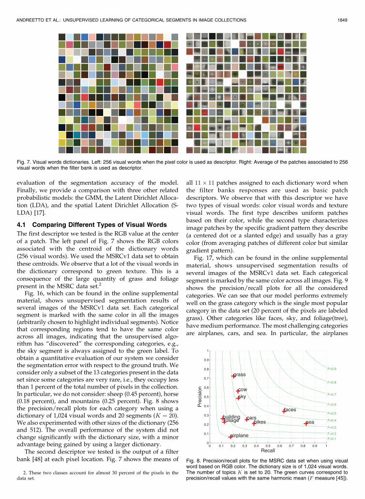
The first descriptor we tested is the RGB value at the centerof a patch. The left panel of Fig. 7 shows the RGB colorsassociated with the centroid of the dictionary words(256 visual words). We used the MSRCv1 data set to obtainthese centroids. We observe that a lot of the visual words inthe dictionary correspond to green texture. This is aconsequence of the large quantity of grass and foliagepresent in the MSRC data set.2

Fig. 16, which can be found in the online supplementalmaterial, shows unsupervised segmentation results ofseveral images of the MSRCv1 data set. Each categoricalsegment is marked with the same color in all the images(arbitrarily chosen to highlight individual segments). Noticethat corresponding regions tend to have the same coloracross all images, indicating that the unsupervised algo-rithm has “discovered” the corresponding categories, e.g.,the sky segment is always assigned to the green label. Toobtain a quantitative evaluation of our system we considerthe segmentation error with respect to the ground truth. Weconsider only a subset of the 13 categories present in the dataset since some categories are very rare, i.e., they occupy lessthan 1 percent of the total number of pixels in the collection.In particular, we do not consider: sheep (0.45 percent), horse(0.18 percent), and mountains (0.25 percent). Fig. 8 showsthe precision/recall plots for each category when using adictionary of 1,024 visual words and 20 segments (K ¼ 20).We also experimented with other sizes of the dictionary (256and 512). The overall performance of the system did notchange significantly with the dictionary size, with a minoradvantage being gained by using a larger dictionary.

The second descriptor we tested is the output of a filterbank [48] at each pixel location. Fig. 7 shows the means of

all 11� 11 patches assigned to each dictionary word whenthe filter banks responses are used as basic patchdescriptors. We observe that with this descriptor we havetwo types of visual words: color visual words and texturevisual words. The first type describes uniform patchesbased on their color, while the second type characterizesimage patches by the specific gradient pattern they describe(a centered dot or a slanted edge) and usually has a graycolor (from averaging patches of different color but similargradient pattern).

Fig. 17, which can be found in the online supplementalmaterial, shows unsupervised segmentation results ofseveral images of the MSRCv1 data set. Each categoricalsegment is marked by the same color across all images. Fig. 9shows the precision/recall plots for all the consideredcategories. We can see that our model performs extremelywell on the grass category which is the single most popularcategory in the data set (20 percent of the pixels are labeledgrass). Other categories like faces, sky, and foliage(tree),have medium performance. The most challenging categoriesare airplanes, cars, and sea. In particular, the airplanes


2. These two classes account for almost 30 percent of the pixels in thedata set.

Fig. 8. Precision/recall plots for the MSRC data set when using visualword based on RGB color. The dictionary size is of 1,024 visual words.The number of topics K is set to 20. The green curves correspond toprecision/recall values with the same harmonic mean (F measure [45]).

Fig. 7. Visual words dictionaries. Left: 256 visual words when the pixel color is used as descriptor. Right: Average of the patches associated to 256visual words when the filter bank is used as descriptor.

category is almost never recovered. The problem with theairplanes and cars categories is that they have a wide rangeof appearances and points of view, which makes it difficultfor the A-LDA model to spot their recurrence across imageswithout supervision. The sea category is relatively rarecompared to the others, less than 1 percent of the data set.

For each category we compute the segmentation accu-racy as a measure of the system performance. Following[51], we define the segmentation accuracy for a category asthe number of correctly labeled pixels in that category,divided by the number of pixels labeled in that category ineither the ground truth or the segmentation results(intersection/union metric3). This pixel-based measure hasseveral limitations: It does not take into account multipleinstances of the same object category in a single image andit does not consider the quality of the segment contours.Nonetheless, we decided to use this particular definitionbecause it is a de facto standard for the computer visioncommunity and it has been used to evaluate other(supervised) segmentation/recognition systems [52], [53].Fig. 10a shows the scatter plot of the accuracies for eachcategory when using color visual words and when usingvector quantized filter bank responses. We see that, ingeneral, the filter banks perform better, although for thecows and sea categories, the color visual words performbetter. We also tested a third type of visual words based onthe SIFT descriptor. Since the SIFT descriptor is based onthe intensity gradient, it does not capture color information.In order to also consider color information, we modified themodel of Fig. 6 to have two different visual words perobservation: one derived from color (see previous discus-sion) and one derived from SIFT.4 For a given segment k,visual words of different types are sampled from twoindependent multinomial distributions, �ck (color) and �sk(SIFT). Fig. 10b shows the scatter plot of the accuracieswhen using color/SIFT visual words and when using filterbank visual words. We observe that the filter banks visual

words and the joint color/SIFT ones have similar accuracyresults (close to the diagonal), with the filter banks visualwords performing better for the categories grass, sky, faces,and foliage, and the color/SIFT visual words giving greateraccuracy for building, bikes, and cows. As previouslyobserved, filter bank visual words can be divided into twogroups: color and texture. Since color/SIFT visual wordsalso capture these two patch properties (in a different way),the similarity of segmentation accuracy is not surprising. Inall the following experiments we will always use filter bankvisual words. We also experimented with other collectionsof images, such as the Boston urban area subset of LabelMe[3] and the scene data set used by Oliva and Torralba [50].Figs. 11 and 12 show several examples of categoricalsegments learned from these data sets.

All the experiments considered so far are completelyunsupervised, i.e., neither regions of an image nor wholeimages have any label. If we allow for a certain amount ofsupervision, we can improve the performance over theunsupervised case. For example, we can consider the casewhen we know a priori which objects are present in eachimage of the collection. In this case we share statistics onlybetween images that contain the same object. Fig. 13compares the precision/recall values for the unsupervisedcase (red crosses) and the semi-supervised case (bluecircles). In the first case, all the images in the collectionare segmented together and the model has to determinewhich object is present in each image. In the second case,we segment together only images that contain objects fromthe same category.5 Using this limited information we canachieve much higher precision/recall values on all thecategories we have labeled.

4.2 Comparison with Other Probabilistic Models

We compare the A-LDA model with three alternativemodels. The first model is a simple GMM with the samenumber of components as topics/segments in the A-LDAmodel. To obtain the model we collect all the descriptors ofall the images and estimate the model parameters and theobservation assignment using EM. We observe that, whenestimating the model, we use neither any affinity informa-tion (segmentation cues) nor image membership.

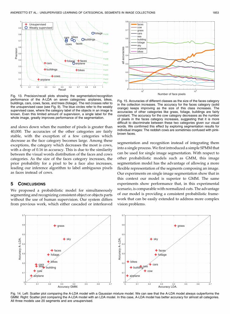
Another possible probabilistic model is the LDA model.As observed in Section 3, this model can be seen as asimplification of the A-LDA model in which the xmn variableis removed. Therefore, the LDA model does not consider therelationship between the visual words of an image (affinitiesinformation), but does consider image membership, i.e., thesame visual word may have different meanings in differentimages. The number of segments is 20 in all the experimentsand a dictionary of 1,024 visual words is used for both theLDA model and A-LDA model. We use filter bank responsesas the descriptor for image patches. Fig. 14 shows scatterplots comparing the A-LDA model with GMM (left) andLDA (right). We see that the A-LDA outperforms GMM onall the categories in the data set. The A-LDA outperforms theLDA in all the categories but two: cars and cows.

We compare our model (A-LDA) with S-LDA proposedby Wang and Grimson [17]. This model extends LDA by


Fig. 9. Precision/recall plots for the MSRC data set when using visualwords based on filter bank responses (red crosses). The dictionary sizeis 1,024 visual words. The number of topics K is set to 20. Theprecision/recall for the spatial latent Dirichlet allocation [17] is alsoreported (black diamonds).

3. Equivalently, the accuracy is given by the equation accuracy ¼true positive

true positive þfalse positive þfalse negative .4. Using only visual words based on SIFT merges categories with similar

texture but different color, like grass and sea.5. We only consider one category for each image. For example, if an

image has both cows and grass, we only consider cows.

considering the proximity of visual words in an image, butwithout using information based on the local similarity ofthe image patches. Table 1, which can be found in the onlinesupplemental material, reports the detection/false alarmrates and the accuracy6 of the two systems. In three out ofthe four categories reported in [17] we obtain higheraccuracy and lower false alarm. For two categories, bikesand faces, we also have higher detection rate. Furthermore,we report results on six categories ignored by Wang andGrimson [17].

Finally, we tested the A-LDA system on the morechallenging MSRCv2 data set. This data set contains a totalof 591 images and 23 categories.7 Since this data set is asuperset of the MSRCv1, we can also observe if and howmuch the segmentation accuracy of the A-LDA decreases

when more categories need to be identified. Besides theusual comparison with the LDA model we also consider thethree supervised segmentation systems described in [52],[53], and [54]; this comparison provides an upper bound onthe performance of the system. The accuracy results arereported in Table 2, which can be found in the onlinesupplemental material. For both the A-LDA model and thebasic LDA we use a dictionary of 1,024 visual wordsobtained from filter bank descriptors and K ¼ 60 topics inthe model.8 We ran the two inference algorithms (Gibbssampling) for approximately the same amount of time. Weobserve that A-LDA outperformed the standard LDA formost categories, with the major exceptions of the categoriesFlower and Book (see the second and third rows of Table 2).Both unsupervised methods had considerable difficulty inrecognizing and segmenting object categories like Cat, Boat,and Body. These categories have a wide range of variabilityand represent only a small fraction of the pixels in the


Fig. 10. Comparison of the segmentation accuracy of the A-LDA model for different types of visual words. (a) Color (RGB) visual words (horizontalaxis) and the filter bank visual words (vertical axis). (b) SIFT visual words (horizontal axis) and the filter bank visual words (vertical axis).

Fig. 11. Four topics/segments learned from the LabelMe database. Each panel contains eight segments from the same topic. The four topicsrepresent four different elements of a possible street scene: “tree/foliage,” “buildings,” “street pavement,” and “sky.” These topic panels show theconsistency we obtain across the images of the collection.

6. The accuracy values for S-LDA were not reported in [17]. Weestimated them from the Detection and False alarm rates reported in [17]and ground truth by calculating, for each category, the number of truepositive, false positive, false negative, and true negative.

7. Two categories, horse and mountains, were not consider in theexperiments because of the limited number of pixels with those labeled.

8. We used a larger number of topics (K ¼ 60) than we did for theMSRCv1 (K ¼ 20) because of the larger number of categories in the data set.

collection so it is challenging to spot the statistical regularityof their appearance. The same categories are better handledwhen a certain amount of supervision is provided as shownby the bottom three rows of Table 2. For all three methodsboth the visual words and the category model are built in adiscriminative way. It is also interesting to compare resultsfor the A-LDA model when applied to the MSRCv1 subsetof images. We see that accuracy is lower for the morechallenging MSRCv2. This is a consequence of the largernumber of categories the system is trying to identify. Forcategories with a large number of observations like Grass,Trees, Bicycle, Sky, and Water the segmentation accuracy iscomparable if not larger. For these categories, the data setprovides enough evidence for building a good statisticalmodel. This observation is further analyzed in Section 4.3.

Of course, even for the grass category (which is thelargest in both the MSRCv1 and MSRCv2), the performanceof the A-LDA is lower than the corresponding one for thesupervised methods. These methods use a large amount ofsupervision, as seen [54]. Those results were obtained using276 training images with pixel level labeling. More complexdata sets like the Pascal VOC were not considered forexperimental evaluation. These data sets were designed tobe challenging for supervised systems, and will be almostimpossible for the unsupervised case.9 Even a relatively

“easy” data set for supervised recognition MSRCv2 is quitechallenging for the unsupervised methods like A-LDA.

4.3 Accuracy versus Category Sample Size

Since our model (Fig. 6) is completely unsupervised, it hasto rely on the co-occurrences of visual words wmn to identifydifferent categories. Therefore, we expect that the larger thenumber of pixels in a category, the higher the accuracy willbe for that category since there is more evidence to identifyco-occurring visual words in that category. To verify thisintuition, we consider the MSRC data set, remove all theimages of faces, and progressively add new images fromthe faces category in the Caltech101 data set.10 In eachiteration, we add a new batch of 10 images to the collection,then run our inference algorithm to obtain the categoricalsegments and compute the accuracies for the faces as wellas all the other categories in the data sets.

Fig. 15 shows the mean accuracies of each category in thedata set for different number of pixels in the facescategory.11 As expected the accuracy for the faces category,depicted with thick solid orange, increases as its sizeincreases. In particular, the accuracy increases faster at thebeginning, when the number of pixels is relatively small


Fig. 12. Six topics/segments learned from the Scene database. Each panel contains eight segments from the same topic. Our visual words

representation incorporates color information; therefore, skies were assigned to two topics, light blue and dark blue.

9. If the recognition accuracy is very low for all the unsupervisedmethods tested, it would be difficult to draw any conclusion.

10. The 30 images in the MSRC data set with face labels are a subset ofthe faces category of the Caltech101.

11. We repeat this experiment 20 times. Each time we randomly selectthe batch of 10 images to add from the list of unused images.

and slows down when the number of pixels is greater than40,000. The accuracies of the other categories are fairlystable, with the exception of a few categories whichdecrease as the face category becomes large. Among theseexceptions, the category which decreases the most is cows,with a drop of 0.16 in accuracy. This is due to the similaritybetween the visual words distribution of the faces and cowscategories. As the size of the faces category increases, theprior probability for a pixel to be a face also increases,leading our inference algorithm to label ambiguous pixelsas faces instead of cows.

5 CONCLUSIONS

We proposed a probabilistic model for simultaneouslysegmenting and recognizing consistent object or objects partswithout the use of human supervision. Our system differsfrom previous work, which either cascaded or interleaved

segmentation and recognition instead of integrating them

into a single process. We first introduced a simple SPMM that

can be used for single image segmentation. With respect to

other probabilistic models such as GMM, this image

segmentation model has the advantage of allowing a more

flexible representation of the segments composing an image.

Our experiments on single image segmentation show that in

this context our model is superior to GMM. The same

experiments show performance that, in this experimental

scenario, is comparable with normalized cuts. The advantage

of our model is providing a consistent probabilistic frame-

work that can be easily extended to address more complex

vision problems.


Fig. 15. Accuracies of different classes as the size of the faces categoryin the collection increases. The accuracy for the faces category (solidorange) keeps improving as the size of this class increases. Theaccuracies of other categories like grass, foliage, buildings are fairlyconstant. The accuracy for the cow category decreases as the numberof pixels in the faces category increases, suggesting that it is moredifficult to discriminate between these two categories given our visualwords. We confirmed this effect by exploring segmentation results forindividual images: The reddish cows are sometimes confused with pink-brown faces.

Fig. 14. Left: Scatter plot comparing the A-LDA model with a Gaussian mixture model. We can see that the A-LDA model always outperforms theGMM. Right: Scatter plot comparing the A-LDA model with an LDA model. In this case, A-LDA model has better accuracy for almost all categories.All three models use 20 segments and are unsupervised.

Fig. 13. Precision/recall plots showing the segmentation/recognitionperformance of the A-LDA on seven categories: airplanes, bikes,buildings, cars, cows, faces, and trees (foliage). The red crosses refer tothe unsupervised case (see Fig. 9). The blue circles refer to the weaklysupervised case, where the category label of the objects in an image isknown. Even this limited amount of supervision, a single label for thewhole image, greatly improves performance of the segmentation.

We extended the single image model to approach themore challenging problems of simultaneous segmentationand recognition of an entire image collection, with limited orno supervision. We found that sharing information about theshape and appearance of a segment across a collection ofimages of objects belonging to the same category can improveperformance. To address the more general case of thesimultaneous unsupervised segmentation and recognitionof multiple categories in a collection of images, we furtherextended our model by also using visual words to describerecurring categorical segments in different images. Thestatistics of the visual words in each segment are sharedacross images, helping the segmentation process and auto-matically discovering recurring elements in the imagecollection. Our experiments show that our model (A-LDAmodel) outperforms other probabilistic models such asGMM, LDA, and S-LDA. We also show how a limitedamount of supervision, namely, the label of the object presentin an image, can greatly improve the segmentation results.Finally, we studied the relation between the performance andthe number of observations in a given category and foundthat the accuracy increases with the number of observations.

In our experiments we considered observations sampledfrom a regular grid in the image. An alternative approachthat can be pursued is the use of superpixels [55] asobservations. This would result in a reduction of the numberof observations and a corresponding speedup of the system.

While A-LDA outperforms the other unsupervisedmodels, its accuracy in a challenging data set like theMSRCv2 is low in absolute terms and quite distant from theresults achieved by the supervised methods. The lack ofsupervision makes the recognition/segmentation problemconsiderably more difficult. However, the gap between thesupervised methods and the A-LDA model is also a resultof the assumptions of the model, in particular theindependence assumption of visual words and observationsand the common topic model for all the segments from thesame category (see [56] for a in-depth discussion on theissue). We believe that our model can offer a starting pointfor investigating more complex descriptions of how imagescan be segmented and objects recognized.

ACKNOWLEDGMENTS

The authors would like to thank Greg Griffin and KristinBranson for reviewing the manuscript and giving manyimportant suggestions for improving it. Funding for thisresearch was provided by ONR-MURI Grant N00014-06-1-0734. Lihi Zelnik-Manor is supported by FP7-IRG grant2009783.

REFERENCES

[1] D. Marr, Vision: A Computational Investigation into the HumanRepresentation and Processing of Visual Information. Henry Holt andCo., Inc., 1982.

[2] J. Malik, S. Belongie, T. Leung, and J. Shi, “Contour and TextureAnalysis for Image Segmentation,” Int’l J. Computer Vision vol. 43,no. 1, pp. 7-27, 2001.

[3] B.C. Russell, A.A. Efros, J. Sivic, W.T. Freeman, and A. Zisserman,“Using Multiple Segmentations to Discover Objects and TheirExtent in Image Collections,” Proc. IEEE Conf. Computer Vision andPattern Recognition, 2006.

[4] L. Cao and L. Fei-Fei, “Spatially Coherent Latent Topic Model forConcurrent Object Segmentation and Classification,” Proc. 11thIEEE Int’l Conf. Computer Vision, 2007.

[5] B. Leibe, A. Leonardis, and B. Schiele, “Combined ObjectCategorization and Segmentation with an Implicit Shape Model,”Proc. Workshop Statistical Learning in Computer Vision, pp. 17-32,May 2004.

[6] E. Borenstein and S. Ullman, “Class-Specific, Top-Down Segmen-tation,” Proc. Seventh European Conf. Computer Vision-Part II,pp. 109-124, 2002.

[7] M. Weber, M. Welling, and P. Perona, “Unsupervised Learning ofModels for Recognition,” Proc. Sixth European Conf. ComputerVision-Part I, pp. 18-32, 2000.

[8] P. Viola and M.J. Jones, “Robust Real-Time Face Detection,” Int’lJ. Computer Vision, vol. 57, no. 2, pp. 137-154, 2004.

[9] D.G. Lowe, “Distinctive Image Features from Scale-InvariantKeypoints,” Int’l J. Computer Vision, vol. 60, no. 2, pp. 91-110, 2004.

[10] R. Fergus, P. Perona, and A. Zisserman, “Object Class Recognitionby Unsupervised Scale-Invariant Learning,” Proc. IEEE Conf.Computer Vision and Pattern Recognition, 2003.

[11] L. Fei-Fei and P. Perona, “A Bayesian Hierarchical Model forLearning Natural Scene Categories,” Proc. IEEE Conf. ComputerVision and Pattern Recognition, vol. 2, pp. 524-531, 2005.

[12] T. Leung and J. Malik, “Representing and Recognizing the VisualAppearance of Materials Using Three-Dimensional Textons,” Int’lJ. Computer Vision, vol. 43, no. 1, pp. 29-44, 2001.

[13] D.M. Blei, A.Y. Ng, and M.I. Jordan, “Latent Dirichlet Allocation,”J. Machine Learning Research, vol. 3, pp. 993-1022, 2003.

[14] M. Vidal-Naquet and S. Ullman, “Object Recognition withInformative Features and Linear Classification,” Proc. Ninth IEEEInt’l Conf. Computer Vision, pp. 281-288, 2003.

[15] G. Dorko and C. Schmid, “Selection of Scale-Invariant Parts forObject Class Recognition,” Proc. Ninth IEEE Int’l Conf. ComputerVision, pp. 634-639, 2003.

[16] A. Rabinovich, A. Vedaldi, C. Galleguillos, E. Wiewiora, and S.Belongie, “Objects in Context,” Proc. 11th IEEE Int’l Conf. ComputerVision, 2007.

[17] X. Wang and E. Grimson, “Spatial Latent Dirichlet Allocation,”Proc. Advances in Neural Information Processing Systems, 2007.

[18] Z. Tu and S.-C. Zhu, “Image Segmentation by Data-DrivenMarkov Chain Monte Carlo,” IEEE Trans. Pattern Analysis andMachine Intelligence, vol. 24, no. 5, pp. 657-673, May 2002.

[19] P. Orbanz and J.M. Buhmann, “Nonparametric Bayesian ImageSegmentation,” Int’l J. Computer Vision, vol. 77, pp. 25-45, 2007.

[20] J. Shi and J. Malik, “Normalized Cuts and Image Segmentation,”IEEE Trans. Pattern Analysis and Machine Intelligence, vol. 22, no. 8,pp. 888-905, Aug. 2000.

[21] N. Ahuja and S. Todorovic, “Learning the Taxonomy and Modelsof Categories Present in Arbitrary Images,” Proc. 11th IEEE Int’lConf. Computer Vision, 2007.

[22] M. Andreetto, L. Zelnik-Manor, and P. Perona, “Non-ParametricProbabilistic Image Segmentation,” Proc. 11th IEEE Int’l Conf.Computer Vision, 2007.

[23] M.I. Jordan, “Graphical Model,” Statistical Science, vol. 19, no. 1,pp. 140-155, 2004.

[24] D. Comaniciu and P. Meer, “Mean Shift: A Robust ApproachToward Feature Space Analysis,” IEEE Trans. Pattern Analysis andMachine Intelligence, vol. 24, no. 5, pp. 603-619, May 2002.

[25] R.O. Duda, P.E. Hart, and D.G. Stork, Pattern Classification, seconded. Wiley-Interscience, 2000.

[26] A. Ng, M.I. Jordan, and Y. Weiss, “On Spectral Clustering:Analysis and an Algorithm,” Proc. Advances in Neural InformationProcessing Systems, 2001.

[27] C. Carson, S. Belongie, H. Greenspan, and J. Malik, “Blobworld:Image Segmentation Using Expectation-Maximization and ItsApplication to Image Querying,” IEEE Trans. Pattern Analysisand Machine Intelligence, vol. 24, no. 8, pp. 1026-1038, Aug. 2002.

[28] R. Kannan, S. Vempala, and A. Vetta, “On Clusterings: Good, Badand Spectral,” J. ACM, vol. 51, no. 3, pp. 497-515, 2004.

[29] R. Zass and A. Shashua, “A Unifying Approach to Hard andProbabilistic Clustering,” Proc. 10th IEEE Int’l Conf. ComputerVision , vol. 1, pp. 294-301, Oct. 2005.

[30] M. Meila and J. Shi, “Learning Segmentation by Random Walks,”Proc. Advances in Neural Information Processing Systems, pp. 873-879, 2000.

[31] S.X. Yu and J. Shi, “Segmentation Given Partial GroupingConstraints,” IEEE Trans. Pattern Analysis and Machine Intelligence,vol. 26, no. 2, pp. 173-183, Feb. 2004.

[32] L. Wasserman, All of Nonparametric Statistics. Springer, 2006.


[33] L. Zelnik-Manor and P. Perona, “Self-Tuning Spectral Clustering,”Proc. Advances in Neural Information Processing Systems, pp. 1601-1608, 2005.

[34] T. Brox, B. Rosenhahn, D. Cremers, and H.-P. Seidel, “Nonpara-metric Density Estimation with Adaptive, Anisotropic Kernels forHuman Motion Tracking,” Proc. Workshop Human Motion in IEEEInt’l Conf. Computer Vision, pp. 152-165, 2007.

[35] T. Cour, F. Benezit, and J. Shi, “Spectral Segmentation withMultiscale Graph Decomposition,” Proc. IEEE CS Conf. ComputerVision and Pattern Recognition, vol. 2, pp. 1124-1131, 2005.

[36] M.D. Escobar and M. West, “Bayesian Density Estimation andInference. Using Mixtures,” J. Am. Statistical Assoc., vol. 90,pp. 577-588, 1995.

[37] C.M. Bishop, Neural Networks for Pattern Recognition. Oxford Univ.Press, 1995.

[38] C.R. Genovese and L. Wasserman, “Rates of Convergence for theGaussian Mixture Sieve,” Annals of Statistics, vol. 28, no. 4,pp. 1105-1127, 2000.

[39] Y.W. Teh, M.I. Jordan, M.J. Beal, and D.M. Blei, “HierarchicalDirichlet Processes,” J. Am. Statistical Assoc., vol. 101, no. 476,pp. 1566-1581, Dec. 2006.

[40] A. Lee, D. Mumford, and J. Huang, “Occlusion Models for NaturalImages: A Statistical Study of a Scale-Invariant Dead LeavesModel,” Int’l J. Computer Vision, vol. 41, nos. 1/2, pp. 7-27, 2001.

[41] E.B. Sudderth and M.I. Jordan, “Shared Segmentation of NaturalScenes Using Dependent Pitman-yor Processes,” Proc. Advances inNeural Information Processing Systems, 2008.

[42] R. Casella, Monte Carlo Statistical Methods. Springer, 1999.[43] S. Lazebnik, C. Schmid, and J. Ponce, “A Maximum Entropy

Framework for Part-Based Texture and Object Recognition,” Proc.10th IEEE Int’l Conf. Computer Vision, vol. 1, pp. 832-838, Oct. 2005.

[44] R. Jin, C. Ding, and F. Kang, “A Probabilistic Approach forOptimizing Spectral Clustering,” Proc. Advances in Neural Informa-tion Processing Systems, 2005.

[45] C. Van Rijsbergen, Information Retrieval, second ed. Butterworth,1979.

[46] J. Sivic, B.C. Russell, A.A. Efros, A. Zisserman, and W.T. Freeman,“Discovering Objects and Their Location in Images,” Proc. 10thIEEE Int’l Conf. Computer Vision, 2005.

[47] E.B. Sudderth, A. Torralba, W.T. Freeman, and A.S. Willsky,“Learning Hierarchical Models of Scenes, Objects, and Parts,”Proc. 10th IEEE Int’l Conf. Computer Vision, pp. 1331-1338, 2005.

[48] J. Winn, A. Criminisi, and T. Minka, “Object Categorization byLearned Universal Visual Dictionary,” Proc. 10th IEEE Int’l Conf.Computer Vision, 2005.

[49] A. Criminisi, “Microsoft Research Cambridge Object RecognitionImage Database, Version 1.0,” 2004.

[50] A. Oliva and A. Torralba, “Modeling the Shape of the Scene: AHolistic Representation of the Spatial Envelope,” Int’l J. ComputerVision, vol. 42, pp. 145-175, 2001.

[51] M. Everingham, L. Van Gool, C.K.I. Williams, J. Winn, and A.Zisserman, “The PASCAL Visual Object Classes Challenge2009 (VOC 2009) Results,” http://www.pascal-network.org/challenges/VOC/voc2009/workshop/index.html. 2012.

[52] J. Verbeek and B. Triggs, “Region Classification with Markov FieldAspect Models,” Proc. IEEE Conf. Computer Vision and PatternRecognition, pp. 1-8, June 2007.

[53] J. Shotton, J.M. Winn, C. Rother, and A. Criminisi, “Textonboostfor Image Understanding: Multi-Class Object Recognition andSegmentation by Jointly Modeling Texture, Layout, and Context,”Int’l J. Computer Vision, vol. 81, no. 1, pp. 2-23, 2009.

[54] J. Shotton, M. Johnson, and R. Cipolla, “Semantic Texton Forestsfor Image Categorization and Segmentation,” Proc. IEEE Conf.Computer Vision and Pattern Recognition, pp. 1-8, June 2008.

[55] X. Ren and J. Malik, “Learning a Classification Model forSegmentation,” Proc. Ninth IEEE Int’l Conf. Computer Vision,pp. 10-17, 2003.

[56] M. Andreetto, “Unsupervised Learning of Categorical Segmentsin Image Collections,” PhD thesis, Dept. of Electrical Eng.,California Inst. of Technology, 2011.

[57] G.C.G. Wei and M.A. Tanner, “A Monte Carlo Implementation ofthe EM Algorithm and the Poor Man’s Data AugmentationAlgorithms,” J. Am. Statistical Assoc., vol. 85, no. 411, pp. 699-704,1990.

Marco Andreetto received the BSc degree incomputer engineering from the University ofPadua in 2001 (summa cum laude) and the MScand PhD degrees from the California Institute ofTechnology in 2005 and 2011, respectively.After graduation he joined Google, Inc., wherehe is currently a member of the Visual SearchTeam. His research interests include visualrecognition, unsupervised learning, statisticalmodeling, Bayesian methods, and large scale

computer vision systems.

Lihi Zelnik-Manor received the BSc degree inmechanical engineering from the Technion in1995, where she graduated summa cum laude,and the MSc (with honors) and PhD degrees incomputer science from the Weizmann Instituteof Science in 1998 and 2004, respectively. Aftergraduating, she worked as a postdoctoral fellowin the Department of Engineering and AppliedScience at the California Institute of Technology(Caltech). Since 2007, she has been a senior

lecturer in the Electrical Engineering Department at the Technion. Herresearch focuses on the analysis of dynamic visual data, including videoanalysis and visualizations of multiview data. Her awards and honorsinclude the Israeli high-education planning and budgeting committee(Vatat) three-year scholarship for outstanding PhD students, and theSloan-Swartz postdoctoral fellowship. She also received the bestStudent Paper Award at the IEEE Shape Modeling InternationalConference 2005 and the AIM@SHAPE Best Paper Award 2005. Sheis a member of the IEEE.

Pietro Perona is the Allen E. Puckett Professorof Electrical Engineering at Caltech. He hascontributed to the theory of partial differentialequations for image processing (anisotropicdiffusion), modeling, and implementing earlyvision processes, to modeling and learningvisual categories (the constellation model). Heis currently interested in visual categorization,the analysis of behavior, and Visipedia.

. For more information on this or any other computing topic,please visit our Digital Library at www.computer.org/publications/dlib.


Date post:	03-Oct-2016
Category:	Documents
Upload:	pietro
View:	213 times
Download:	1 times

Unsupervised Learning of Categorical Segments in Image Collections

Documents