Unwritten Procedural Modeling with the Straight Skeleton This thesis has been composed by the student — Tom Kelly Submitted in fulfilment of the requirements for the degree of Doctor of Philosophy School of Computing Science College of Science and Engineering May 2013 c Tom Kelly. All contents not marked c other parties is released under the Creative Commons - BY 3.0 license Available online http://goo.gl/whgo6j
Transcript
Unwritten Procedural Modelingwith the Straight Skeleton
This thesis has been composed by the student —
Tom Kelly
Submitted in fulfilment of the requirements for the degree of
5.53 Comparison of PEs with previous systems . . . . . . . . . . . . . . . . 204
5.54 The PE as an automated data-loss system . . . . . . . . . . . . . . . . 205
A.1 The source material for interactive evaluation . . . . . . . . . . . . . . 215
1
Chapter 1
Introduction
1.1 Motivation
Figure 1.1: Hour glasses at the London Science Museum.
We may ask ourselves how we would create a single model that could create all of
the hour glasses in Figure 1.1. This is the goal in procedural geometric modeling –
we have no definitive way to do this today, but in this document we hope to take
some steps towards a solution.
Whilst a standard 3D work flow might allow a user to create a single hour glass
of a specific dimension and design, a procedural modeling system might let a user
create an algorithm that produces a glass of any given dimension.
Procedural geometric modeling (PGM ) is a field studying algorithms that compute
geometry. A procedural model consists of a sequence of parametrised operations that
are able to automatically construct a variety of geometric forms.
The additional level of abstraction offered by PGM has significant benefits over single-
instance modeling, but introduces a number of challenges. The advantages of PGM
1.1. Motivation 2
include:
• An arbitrary quantity of geometry can be created to describe a virtual environ-
ment in constant time; the time it takes to construct the procedural model.
• The removal of the existing restriction that the size of a virtual environment is
proportional to the time spent creating it.
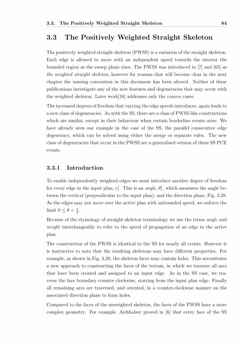
• The quality of the environment is consistent at no additional cost.
• Procedural geometry tools could lead to runtime environment generation. A
virtual world can be generated as the user explores it, giving an experience with
more variety and less repetition to the user [97].
• Procedural methods offers the potential to generate content that reacts to various
stimuli. For example it could respond to current hardware availability, to users’
level of expertise, the length of their attention span, or the medium on which it
is presented.
One particular application that has become a testbed for the concepts of PGM is urban
modeling. In 2010, half of the people in the world lived in cities, and this fraction is
increasing. Cities form the backdrops to large portions of our lives; the way they
are designed, how they look, how we think about them, and how we get around them
directly affects us all. With the rise of computer graphics, creating cityscapes in virtual
worlds has become a common task in a wide range of disciplines such as architecture,
city planning, 3D cartography, video games and cinema.
However, creating virtual representations of cityscapes is expensive. At the crudest
level, paying an artist to attach a door-handle to every door in every building in a
town is costly. Alternately we may obtain 3D city geometry by reconstructing pho-
tographs, but obtaining the photos is difficult, and the results often have a lot of noise.
Furthermore, the cities that we wish to model may not yet exist, may have only existed
before the invention of photography, or be entirely fictional. PGM offers a solution to
these issues by promising to generate large quantities of characteristic geometry very
quickly. The real world applications of urban procedural modeling are growing, recent
examples include —
• Masdar is a new city, designed and built entirely on undeveloped land outside
Abu Dhabi. The initial project is intended to be completed in 2015 and will cover
106m2[266]. Given the large quantity of architecture that had to created, one of
the designers turned to PGM, in the form of CityEngine[66] to design the Swiss
Quarter of the city[67].
1.1. Motivation 3
• Video games can use procedural technology to create new locations as the player
explores. For example Dwarf Fortress [78] generates the terrain, structures and
inhabitants of a virtual world procedurally. In this situation the key advantage is
that a player may continually explore and discover unique structures, that neither
they, nor anyone else, have seen before.
• When the first Superman movie was filmed in 1978 computer graphics were in
their infancy. To give the appearance of Superman flying, Christopher Reeve was
composited on top of footage from New York City, as a stand in for the fictional
city of Metropolis. In contrast the 2013 release of Man of Steel portrayed the
same fictional city, this time generated using the PGM tools Houdini[219] and
CityEngine[103]. The advantages of PGM in this situation is that an entirely
unrecognisable yet realistic fictional city could be created. Additionally, because
the model was digital it could be realistically destroyed by a physical simulation
of the alien invaders.
Given the promise of PGM, it makes sense to question why it isn’t the standard tech-
nique for geometry creation. Designing procedural models is more complex; the de-
signer must not just design a single item of geometry, but a continuum. Current
state-of-the-art systems rely extensively on programming paradigms for users to con-
struct useful and powerful procedural models. In summary, the drawbacks of current
PGM include —
• Designers must undertake the more complex task of designing a class of geometry,
rather than a single instance.
• Traditional artists are not familiar with classical methods of describing algo-
rithms, such as programming languages.
• Traditional software engineers do not possess a classically trained sense of aes-
thetic.
• There are a large number of use cases of PGM, with each likely to require different
solutions.
In this thesis we are concerned with removing several of these drawbacks, specifically
the requirement that current PGM systems require considerable programming exper-
tise.
1.2. Hypothesis 4
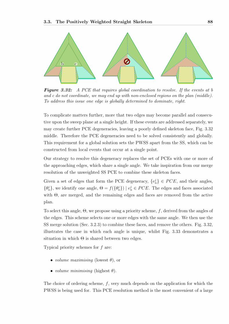
1.2 Hypothesis
We propose that a geometric construct, the straight skeleton, and its generalisations,
are a powerful technique for the creation of PGM systems that are accessible to people
without programming skills. Systems exploiting these skeletons and variations thereof
are able to generate large scale, varied and highly realistic results within the domain
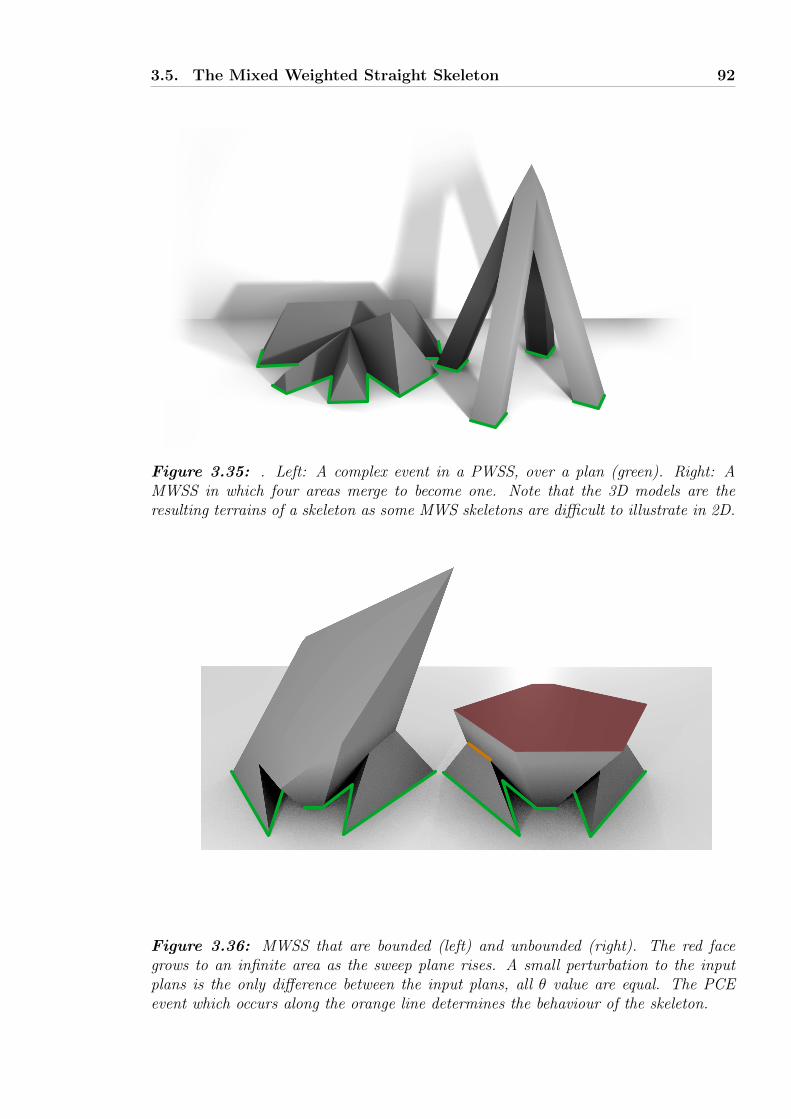
of urban procedural modeling.
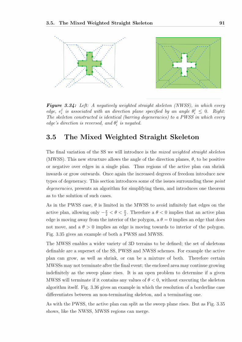
1.3 Contributions
Our contributions to the corpus while examining the above hypothesis include:
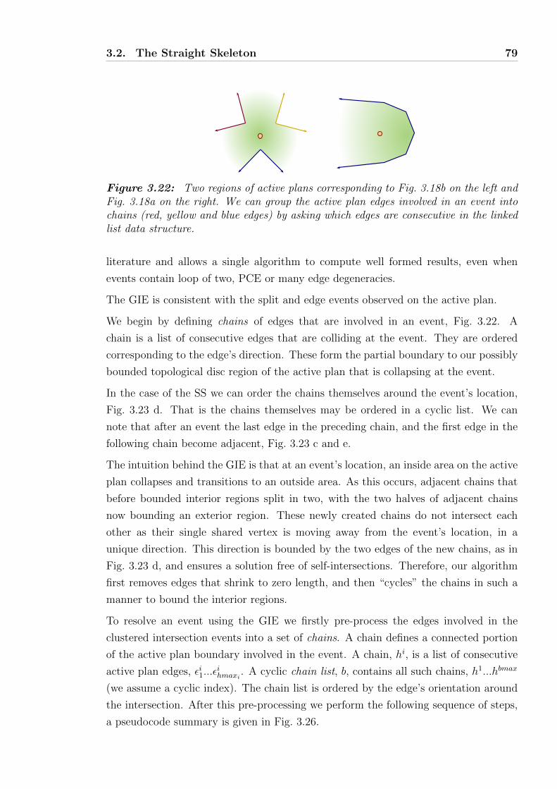
• A simplification of existing straight skeleton events, the generalised intersection
event.
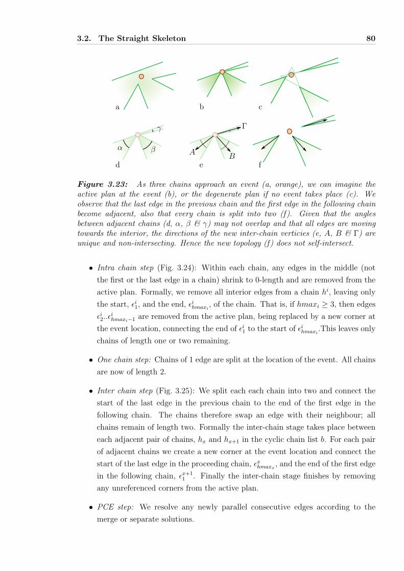
• A novel skeleton, the mixed weighted straight skeleton.
• A method and evaluation of a system for procedural modeling of city lot shapes
using the straight skeleton.
• A method and evaluation for the procedural modeling of architectural shells using
the MWSS.
The papers written in the course of this thesis were:
• Interactive Architectural Modeling with Procedural Extrusions [121]
• Procedural Generation of Parcels in Urban Modeling [252]
1.4 Overview
To lay the ground for this work Chapter 2 examines existing work, and describes the
properties of existing procedural systems. We continue to analyse the straight skeleton
in Chapter 3 and to apply the skeleton to the problem of urban procedural modeling
in Chapters 4 and 5.
The following chapter samples the wide range of tools available for the generation of
3D geometry. In particular we observe that an offset mechanism driven by the straight
skeleton is a powerful accompaniment to a written programming language. This insight
lead us to examine skeletons in greater detail.
1.4. Overview 5
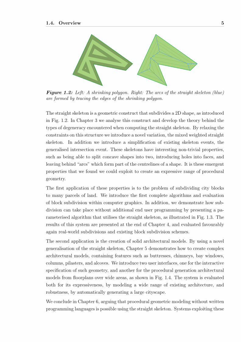
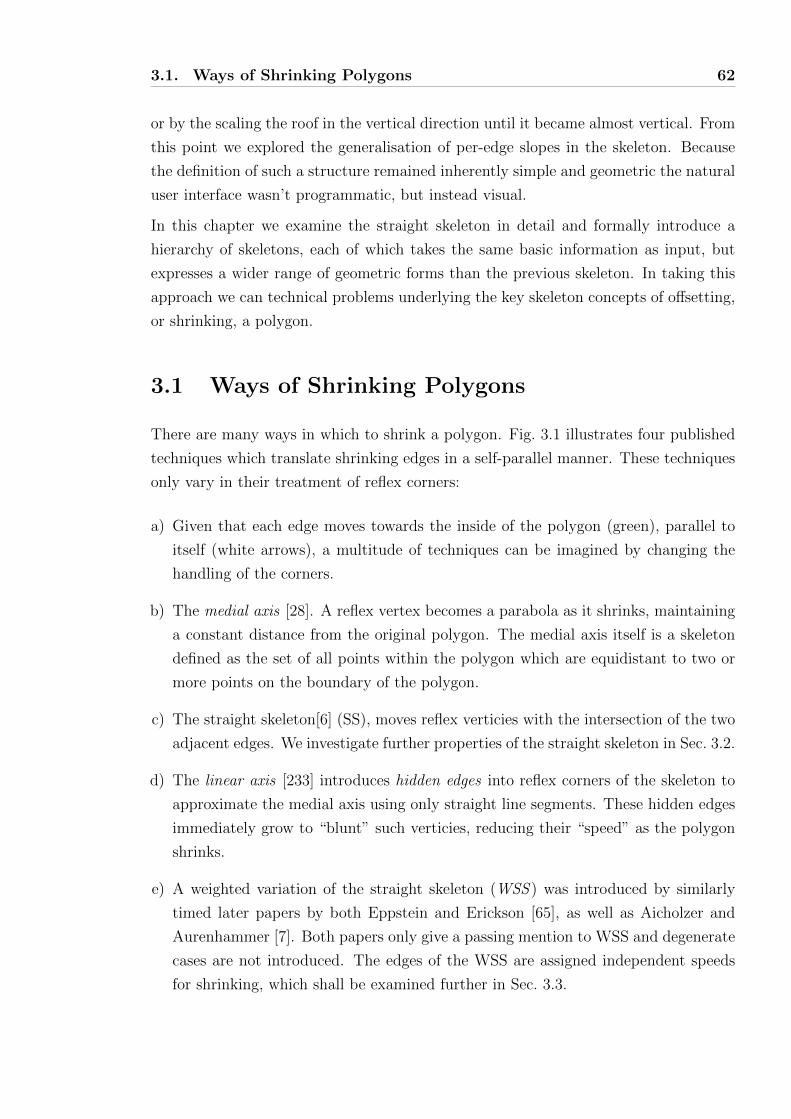
Figure 1.2: Left: A shrinking polygon. Right: The arcs of the straight skeleton (blue)are formed by tracing the edges of the shrinking polygon.
The straight skeleton is a geometric construct that subdivides a 2D shape, as introduced
in Fig. 1.2. In Chapter 3 we analyse this construct and develop the theory behind the
types of degeneracy encountered when computing the straight skeleton. By relaxing the
constraints on this structure we introduce a novel variation, the mixed weighted straight
skeleton. In addition we introduce a simplification of existing skeleton events, the
generalised intersection event. These skeletons have interesting non-trivial properties,
such as being able to split concave shapes into two, introducing holes into faces, and
leaving behind “arcs” which form part of the centrelines of a shape. It is these emergent
properties that we found we could exploit to create an expressive range of procedural
geometry.
The first application of these properties is to the problem of subdividing city blocks
to many parcels of land. We introduce the first complete algorithms and evaluation
of block subdivision within computer graphics. In addition, we demonstrate how sub-
division can take place without additional end user programming by presenting a pa-
rameterised algorithm that utilises the straight skeleton, as illustrated in Fig. 1.3. The
results of this system are presented at the end of Chapter 4, and evaluated favourably
again real-world subdivisions and existing block subdivision schemes.
The second application is the creation of solid architectural models. By using a novel
generalisation of the straight skeleton, Chapter 5 demonstrates how to create complex
architectural models, containing features such as buttresses, chimneys, bay windows,
columns, pilasters, and alcoves. We introduce two user interfaces, one for the interactive
specification of such geometry, and another for the procedural generation architectural
models from floorplans over wide areas, as shown in Fig. 1.4. The system is evaluated
both for its expressiveness, by modeling a wide range of existing architecture, and
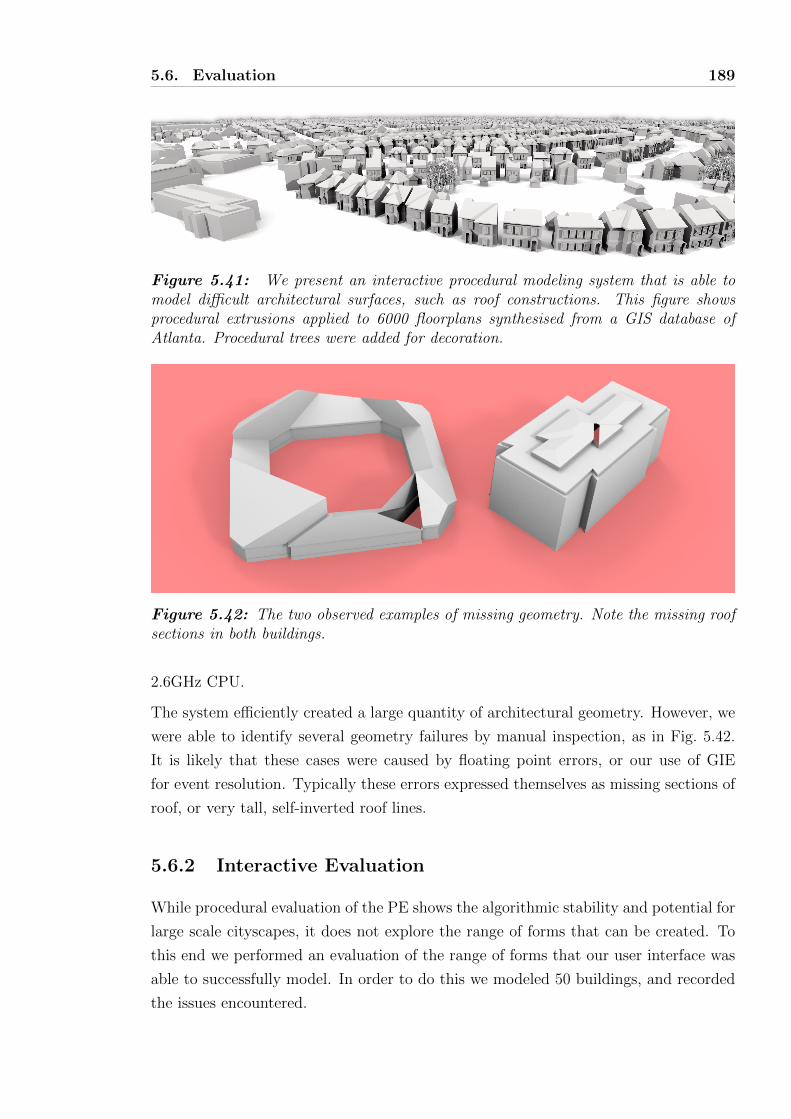
robustness, by automatically generating a large cityscape.
We conclude in Chapter 6, arguing that procedural geometric modeling without written
programming languages is possible using the straight skeleton. Systems exploiting these
1.4. Overview 6
Figure 1.3: The results of our parcel subdivision algorithm within CityEngine. Left:The parcel subdivision generated with both skeleton (bottom left of grey line) and OBB(top right) techniques; the colouring denotes relative area. Right: the result of the urbanprocedural modeling pipeline within CityEngine.
Figure 1.4: We present an interactive procedural modeling system that is able tomodel difficult architectural surfaces, such as roof constructions. This figure showsprocedural extrusions applied to 6000 floorplans synthesised from a GIS database ofAtlanta. Procedural trees were added for decoration.
1.4. Overview 7
skeletons and variations thereof are able to generate large scale, varied, and highly
realistic results within the domain of urban procedural modeling.
8
Chapter 2
Readings: A Spectrum of
Proceduralisation
This chapter introduces some of the technical background of procedural modeling
within the field of graphics. Procedural modeling is a broad subject that borrows
from many established fields; we give an overview of the subject’s context within a
broad spectrum of proceduralisation.
This spectrum leads from general purpose languages to a specific instance of a model.
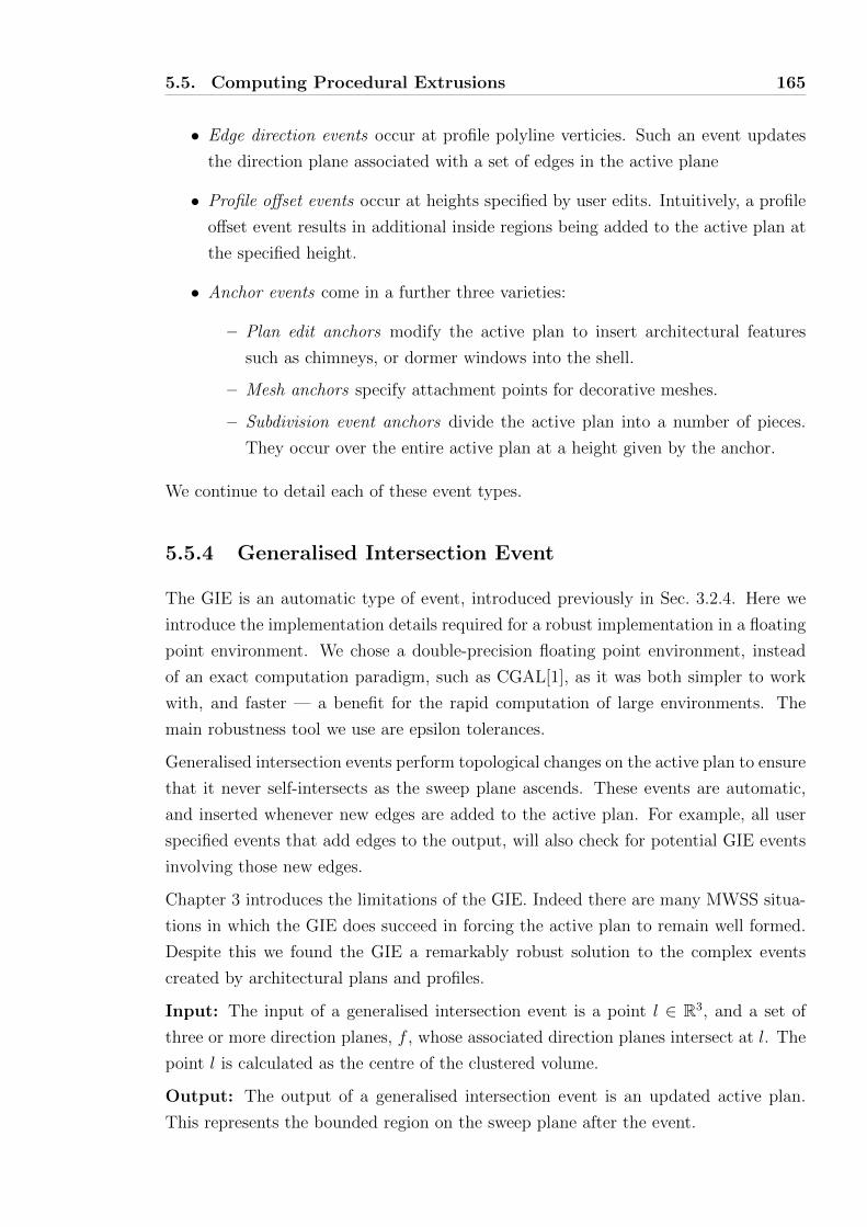
At one extreme we visit general models that are able to create a wide variety of geom-
etry, for example a programming language (not to be confused with a single program
in a language) is capable of creating any geometry we can describe. As we progress
we visit models that only work within a specified domain or produce models similar to
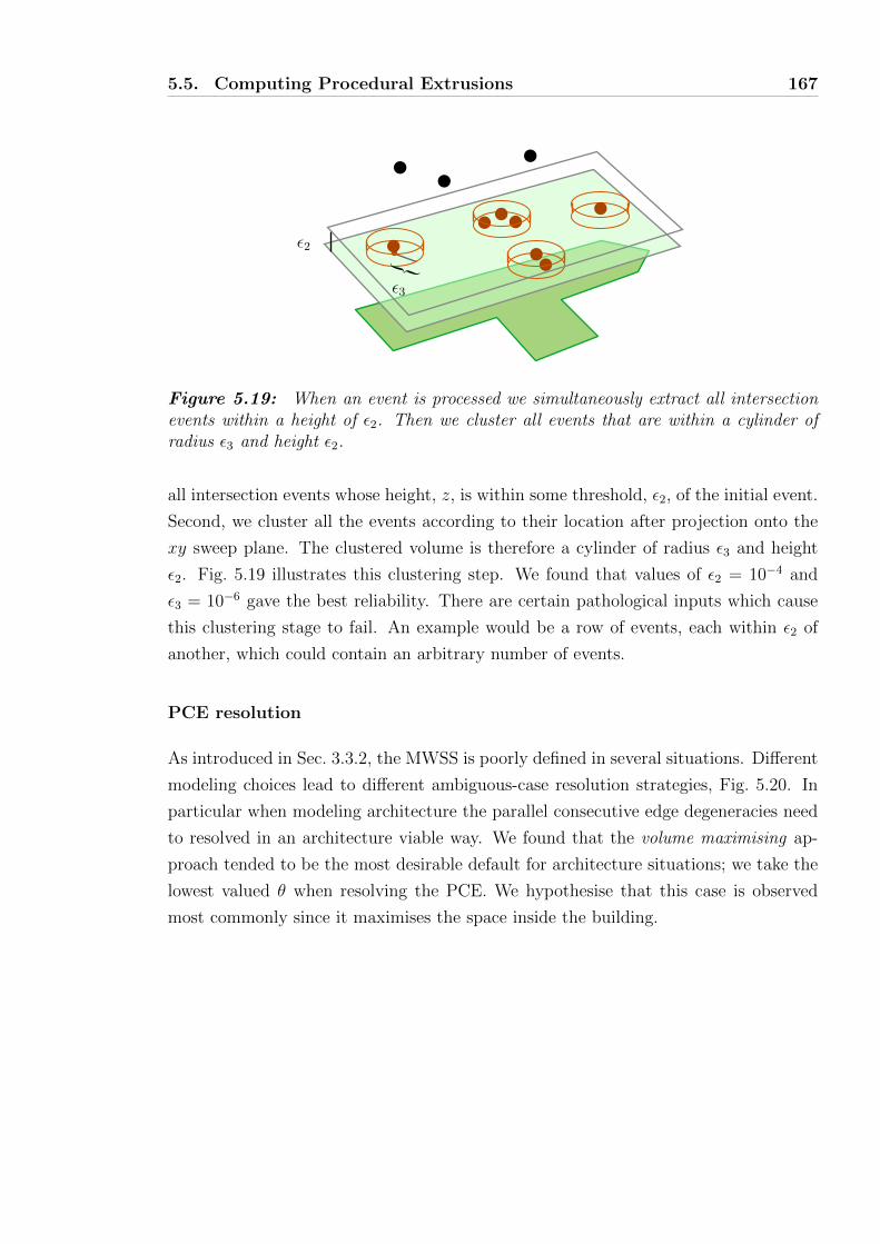
an example. At the most specific end of our spectrum we visit “models” that are only
single instances, such as a 3D mesh of a bunny.
A general language can describe any computable geometry, while an instance is a
single, unchanging, object. However an instance is ready to use, while a language takes
considerable specialisation to create any results. Furthermore, an instance requires no
intelligence on the part of the user and guarantees good results, while a fully general
language requires lots of intelligence and provides no assurances as to the final quality
of the geometry.
In line with the content of the thesis this section will provide an emphasis on those
techniques relevant to urban procedural modeling, although context is provided by
sketches of the surrounding topics. We begin by examining the most general geometry
production systems — languages, grammars and their variants, before moving onto
the more specific combinatory modeling approaches, simulation and inverse procedural
modeling techniques. The most specific techniques form the end of our spectrum —
shape deformation and 3d tools.
2.1. General Purpose Programming Languages 9
public void pa int ( Graphics2D g ){
int count = 1 ;do{
g . r o t a t e ( Math . PI/2 ) ;g . s c a l e ( 1+ ( count /100.) ,1+ ( count / 1 0 0 . ) ) ;for (double d : new double [ ] {0 , Math . PI }){
g . r o t a t e ( d ) ;g . t r a n s l a t e ( −50, 0 ) ;g . draw ( new Arc2D . Double ( −5, −5, 10 , 10 , 90 , 180 , Arc2D .OPEN ) ) ;g . t r a n s l a t e ( 50 , 0 ) ;
}} while ( count++ < 2 0 ) ;
}
Figure 2.1: A small example of a 2D geometric program in Java.
There are two common uses of the word model in PGM — to represent some
system that may create some geometry (“a grammatical model of architecture”),
and to refer to the geometry itself (“the 3D bunny model”). In this chapter we
will attempt to only use the former description, reserving model as a synonym for
system to avoid confusion.
2.1 General Purpose Programming Languages
We first encounter an extreme – the general purpose programming language. Pre-
dominantly these languages are text-string based and Turing complete[245], such as
FORTRAN[114], Haskell[110] or Java[86], Fig. 2.1. Appropriate libraries and inter-
faces allow these languages to create descriptions of geometric objects.
Being general, these languages can describe any computable geometry. However doing
so is quite complex, especially for users unable to write programs. In particular a
random string is most likely not a valid program, while a particular random program
will be unlikely to create geometric output.
There are a wide variety of libraries available to generate geometry via a general pur-
pose programming language. Many of the original library functions were intended
to interface with graphics hardware such as OpenGL[270], others were languages for
realistic rendering, such as RenderMan[247]. More recently higher level interfaces
have emerged such as Open Inventor[262] and the Generative Modeling Language[105]
(GML). Havemann introduced GML to construct procedural graphical primitives via
Euler operations to generate meshes, which may be interrupted as multi-resolution
2.2. Formal String Grammars 10
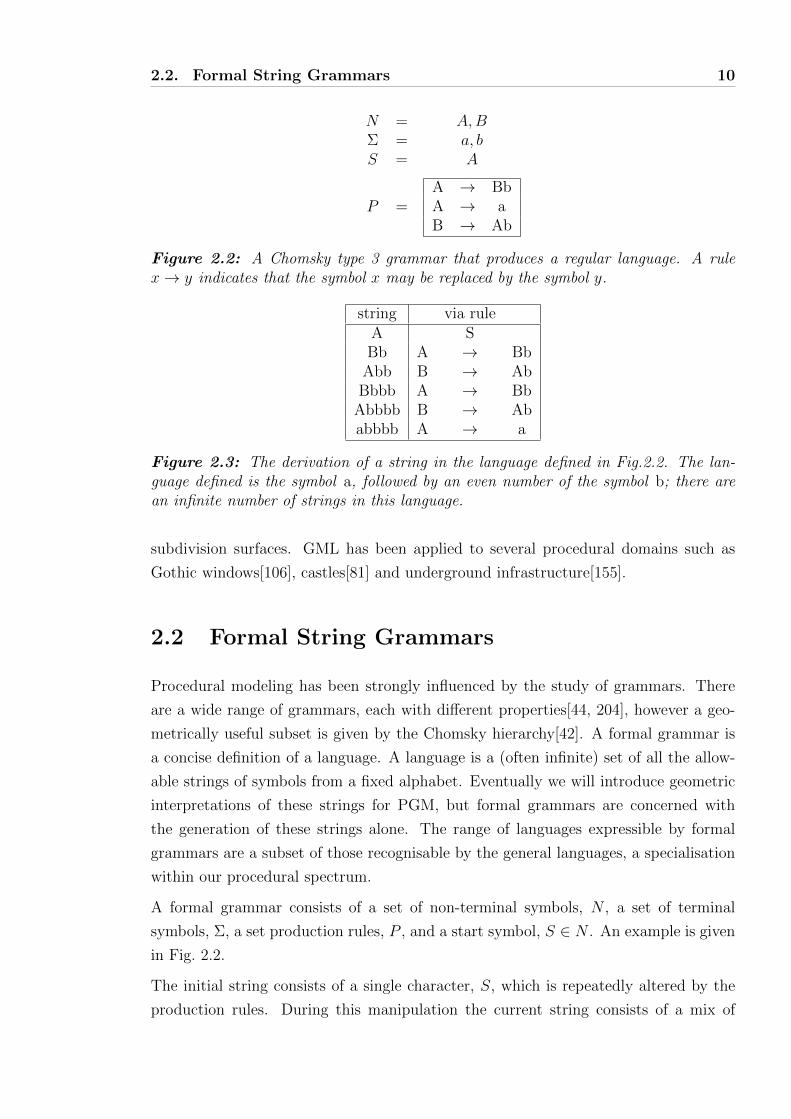
N = A,BΣ = a, bS = A
P =A → BbA → aB → Ab
Figure 2.2: A Chomsky type 3 grammar that produces a regular language. A rulex→ y indicates that the symbol x may be replaced by the symbol y.
string via ruleA SBb A → Bb
Abb B → AbBbbb A → Bb
Abbbb B → Ababbbb A → a
Figure 2.3: The derivation of a string in the language defined in Fig.2.2. The lan-guage defined is the symbol a, followed by an even number of the symbol b; there arean infinite number of strings in this language.
subdivision surfaces. GML has been applied to several procedural domains such as
Gothic windows[106], castles[81] and underground infrastructure[155].
2.2 Formal String Grammars
Procedural modeling has been strongly influenced by the study of grammars. There
are a wide range of grammars, each with different properties[44, 204], however a geo-
metrically useful subset is given by the Chomsky hierarchy[42]. A formal grammar is
a concise definition of a language. A language is a (often infinite) set of all the allow-
able strings of symbols from a fixed alphabet. Eventually we will introduce geometric
interpretations of these strings for PGM, but formal grammars are concerned with
the generation of these strings alone. The range of languages expressible by formal
grammars are a subset of those recognisable by the general languages, a specialisation
within our procedural spectrum.
A formal grammar consists of a set of non-terminal symbols, N , a set of terminal
symbols, Σ, a set production rules, P , and a start symbol, S ∈ N . An example is given
in Fig. 2.2.
The initial string consists of a single character, S, which is repeatedly altered by the
production rules. During this manipulation the current string consists of a mix of
2.3. Graph Grammars 11
Chomsky designation rule format language nametype 3 n1 → σ1 (left) regular
n2 → n3σ2
type 2 n4 → φ•1 context freetype 1 φ•2n5φ
•3 → φ•2φ
•4φ•3 context sensitive
type 0 φ•5 → φ•6 recursively enumerable
Figure 2.4: The Chomsky hierarchy of grammars. σx ∈ Σ, nx ∈ N and φx ∈ Σ ∪N .Repeated elements from a group are marked •.
terminal and non-terminal symbols. When only terminal symbols remain in the string
the production terminates. The final string is a member of the language defined by the
grammar. We evaluate the earlier example in Fig. 2.3.
Different classes of languages can be defined by different forms of production rules.
The example in Fig. 2.2 is a type-3 grammar in the Chomsky hierarchy. A type-3
language may replace a single non-terminal symbol, with either a terminal symbol, or
a non-terminal symbol followed by a terminal.
Type-3 grammars define the set of regular languages. A more expressive grammar may
be allowed to replace the symbol with a longer string (a type-2 language), examine the
context of the single symbol to be replaced (type 1), or replace any string with any
other (type 0). Chomsky named this increasingly powerful hierarchy of grammars as
types 2, 1 and 0, as shown in Fig 2.4. Each expresses a super-set of the languages of
the previous type by relaxing the restrictions on the context of the replaced symbols.
There are a wide variety of other string rewriting systems[124]. For example, if we re-
move the distinction between terminal and non-terminal symbols, and the requirement
for a single starting symbol, then we instead have a semi-Thue process [49]. Another
variation is a parallel grammar, which applies a rule to every symbol in the string with
each iteration. If we use a parallel context sensitive grammar over a symbol set con-
sisting of the binary digits, then we have cellular automata[268], a popular example
of which is Conway’s game of life[80]. 3D cellular automata have been used to create
procedural models of creeping plants[90]. Alternately every production rule in a gram-
mar may manipulate attributes associated with a specific instance of a symbol, leading
to attributed grammars [126]. Finally we may operate on graphs, instead of strings,
leading to the concept of graph-grammars.
2.3 Graph Grammars
Graph Grammars specialise the concept of string grammars to include a topological
element. Instead of replacing a symbol or string, we replace a node or sub-graph of a
2.3. Graph Grammars 12
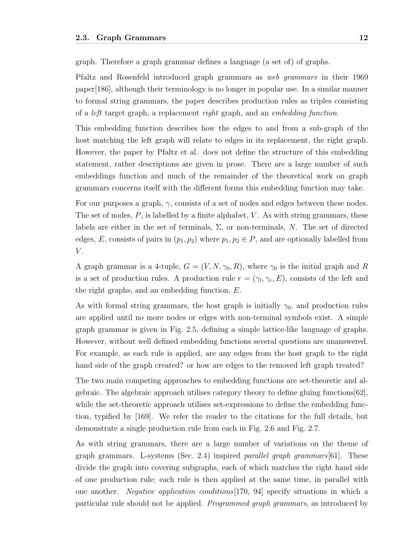
graph. Therefore a graph grammar defines a language (a set of) of graphs.
Pfaltz and Rosenfeld introduced graph grammars as web grammars in their 1969
paper[186], although their terminology is no longer in popular use. In a similar manner
to formal string grammars, the paper describes production rules as triples consisting
of a left target graph, a replacement right graph, and an embedding function.
This embedding function describes how the edges to and from a sub-graph of the
host matching the left graph will relate to edges in its replacement, the right graph.
However, the paper by Pfaltz et al. does not define the structure of this embedding
statement, rather descriptions are given in prose. There are a large number of such
embeddings function and much of the remainder of the theoretical work on graph
grammars concerns itself with the different forms this embedding function may take.
For our purposes a graph, γ, consists of a set of nodes and edges between these nodes.
The set of nodes, P , is labelled by a finite alphabet, V . As with string grammars, these
labels are either in the set of terminals, Σ, or non-terminals, N . The set of directed
edges, E, consists of pairs in (p1, p2) where p1, p2 ∈ P , and are optionally labelled from
V .
A graph grammar is a 4-tuple, G = (V,N, γ0, R), where γ0 is the initial graph and R
is a set of production rules. A production rule r = (γl, γr, E), consists of the left and
the right graphs, and an embedding function, E.
As with formal string grammars, the host graph is initially γ0, and production rules
are applied until no more nodes or edges with non-terminal symbols exist. A simple
graph grammar is given in Fig. 2.5, defining a simple lattice-like language of graphs.
However, without well defined embedding functions several questions are unanswered.
For example, as each rule is applied, are any edges from the host graph to the right
hand side of the graph created? or how are edges to the removed left graph treated?
The two main competing approaches to embedding functions are set-theoretic and al-
gebraic. The algebraic approach utilises category theory to define gluing functions[62],
while the set-theoretic approach utilises set-expressions to define the embedding func-
tion, typified by [169]. We refer the reader to the citations for the full details, but
demonstrate a single production rule from each in Fig. 2.6 and Fig. 2.7.
As with string grammars, there are a large number of variations on the theme of
divide the graph into covering subgraphs, each of which matches the right hand side
of one production rule; each rule is then applied at the same time, in parallel with
one another. Negative application conditions [170, 94] specify situations in which a
particular rule should not be applied. Programmed graph grammars, as introduced by
2.3. Graph Grammars 13
c
a
b
a
b
A
B
a
b
A
B
A
B
C
a
b
a
b
a
b
a
b
a
b
a
b
A
B
a
b
c
a
b
cCinitial host graph, γ0 =
production rules, R =
c
c
cc
c
V = {A,B,C, a, b, c}, N = {A,B,C}
Figure 2.5: Left: an overly simple graph grammar, overlooking embedding rules.Right: several graphs in the language defined by this grammar. Note edge labels are notshown here.
R =
A
B C
a
b c
d
A
B C
a
b c
a
b d
a
b d
a
b c
d
γ0 = = result
1
2 3
1
2 3
1
2 3
Figure 2.6: The application of an set-theoretic production rule, R, using the doublepushout method[62]. Note that numeric values establish node identity in these diagrams.Top row: the two stages in the production rule. Top left: the left graph to match. Topmiddle: any nodes to be renamed have their labels removed and edges to be deleted areremoved. Top right: the new labels and edges are applied. Bottom: the application ofR to a graph (bottom right).
2.3. Graph Grammars 14
γ0 =R =1 2 3 4 5
A a b b a
ri = (5; Rj Li ∪ Li (1)) A
B
C
i
j
i
lj = (B Li (1); 3, 4)
B
Cj
2 3 4 5a b b ai
j j
lj = (B Li (1); 3, 4)
ri = (5; Rj Li ∪ Li (1))
B
Cj
2 3 4 5a b b aiA
B
C
i
j
1
B
B
Cj
2 3 4 5a b b aiA
B
C
i
j
1
B
Cj
2 3 4 5a b b aiA
B
C
i
j
1
B
Cj
2 3 4 5a b b ai
j j
ii
node replacement
Figure 2.7: The application of an algebraic production rule using the system specifiedby Nagl[169]. First row: the rule, R which consists of the left graph, the right graph,and the embedding components lj, ri. Numeric node identities are given outside eachnode in the rule. The graph we will apply the rule to is γ0, replacing the node labelledA with the right graph (second row). Third row: the application of the embedding ljcreates new edges by walking over the graph (dashed arrows). The origin of the walk isthe node with identity 1, traversing all outbound edges labelled i and filtering for nodeslabelled B. The destinations are the nodes with identity 3 and 4, the new edges areshown in bold. The embedding ri proceeds similarly, except the ∪ operator performstwo walks to use as the destinations. The resulting graph is given in the bottom right.
2.4. L-Systems 15
Gottler[88], take this concept further and replace the set of production rules with a list
of production rules to be applied sequentially, via conditional statements or loops.
Unfortunately identifying matching subgraphs in graphs (to identify the portion of
graphs to be replaced) is an instance of the computationally NP-complete subgraph
isomorphism problem. While there are situations where this complexity is alleviated,
such as in the case of planar graphs[64], this complexity may be a reason that graph
grammars are not widely used in PGM. Another problem is that graph grammars are
no more expressive than string grammars as there is an encoding of any graph in string
form (typically an adjacency matrix). This string representation may be manipulated
in equally expressive ways via a type 0 string grammar.
In spite of these shortcomings there are several graphical applications of graph gram-
mars, such as the design of technical diagrams[87], production of system flow dia-
grams [56], the design of a visual languages[91] and CAD-systems[92]. In particular
graph grammars offer a topological-oriented description of the otherwise geometry ori-
ented shape-grammars[279], introduced in Sec. 2.5.
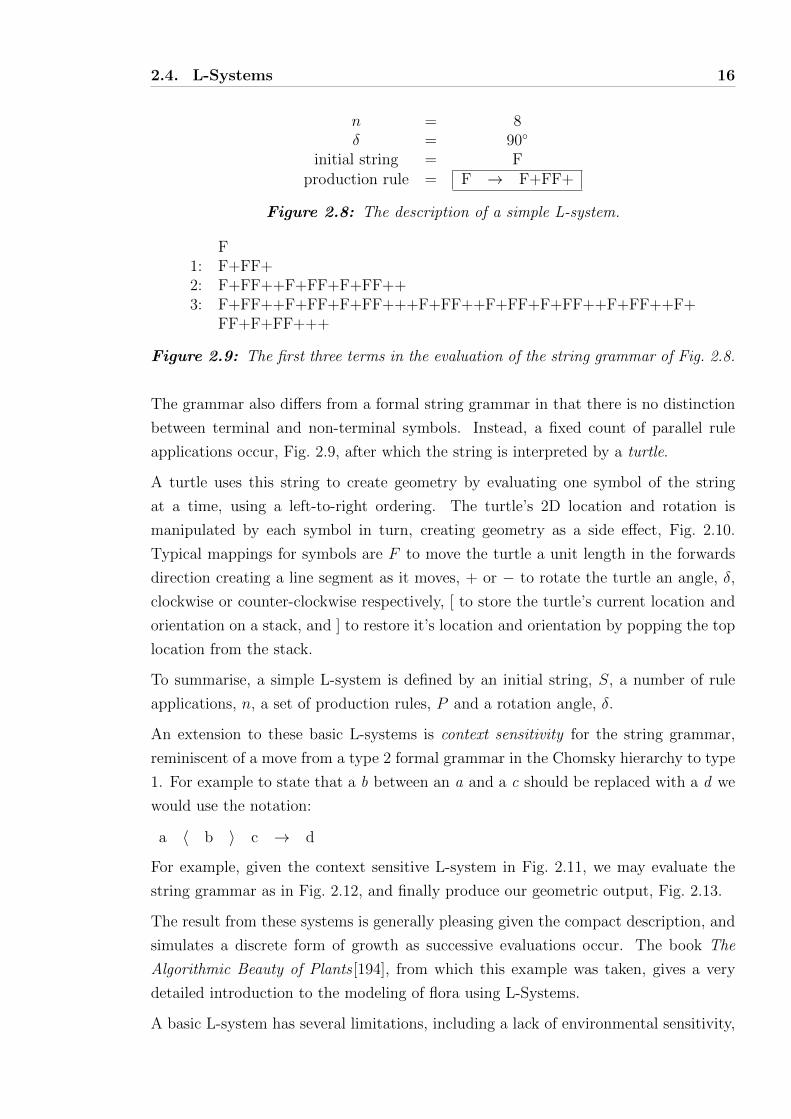
2.4 L-Systems
Lindenmayer-systems [142] introduced a parallel string replacement grammar in 1968,
specifically motivated by the study of plant growth. Unlike the sequential model de-
scribed by Chomsky, every biological cell in a plant may divide simultaneously. To
simulate this, a production rule is applied to every symbol in the string concurrently.
Meanwhile in the 1980’s the computer graphics field was producing tree models, these
were lacking a formal grammar, such as the tendril-like forms in [119], or the detailed
models of specific varieties of trees in [27]. In 1986 L-systems were combined with
graphical techniques[193] to produce a graphical interpretation of a grammar’s lan-
guage. This combination of a string grammar and a turtle became synonymous with
the term L-system. In binding their domain to graphics, and usually botany, L-systems
are a more specialised system than formal grammars, the first true procedural geomet-
ric modeling system we examine.
A basic L-system specifies a parallel string replacement grammar, a number of iter-
ations, a starting string, and a turtle interpreter to create graphical output. Unlike
grammars their output is a single result, rather than a language. We define an example
L-system in Fig. 2.8,
The string replacement grammar doesn’t contain any terminal symbols, and is parallel
in that at every derivation step every symbol in the string is replaced by a matching rule.
Figure 2.9: The first three terms in the evaluation of the string grammar of Fig. 2.8.
The grammar also differs from a formal string grammar in that there is no distinction
between terminal and non-terminal symbols. Instead, a fixed count of parallel rule
applications occur, Fig. 2.9, after which the string is interpreted by a turtle.
A turtle uses this string to create geometry by evaluating one symbol of the string
at a time, using a left-to-right ordering. The turtle’s 2D location and rotation is
manipulated by each symbol in turn, creating geometry as a side effect, Fig. 2.10.
Typical mappings for symbols are F to move the turtle a unit length in the forwards
direction creating a line segment as it moves, + or − to rotate the turtle an angle, δ,
clockwise or counter-clockwise respectively, [ to store the turtle’s current location and
orientation on a stack, and ] to restore it’s location and orientation by popping the top
location from the stack.
To summarise, a simple L-system is defined by an initial string, S, a number of rule
applications, n, a set of production rules, P and a rotation angle, δ.
An extension to these basic L-systems is context sensitivity for the string grammar,
reminiscent of a move from a type 2 formal grammar in the Chomsky hierarchy to type
1. For example to state that a b between an a and a c should be replaced with a d we
would use the notation:
a 〈 b 〉 c → d
For example, given the context sensitive L-system in Fig. 2.11, we may evaluate the
string grammar as in Fig. 2.12, and finally produce our geometric output, Fig. 2.13.
The result from these systems is generally pleasing given the compact description, and
simulates a discrete form of growth as successive evaluations occur. The book The
Algorithmic Beauty of Plants [194], from which this example was taken, gives a very
detailed introduction to the modeling of flora using L-Systems.
A basic L-system has several limitations, including a lack of environmental sensitivity,
2.4. L-Systems 17
n = 1 n = 2 n = 3 n = 4
n = 8
F F+ F+F F+FF F+FF+
Figure 2.10: Top, left-right: incrementally constructing a graphical interpretation ofa string using a turtle. Bottom: the turtle’s evaluation of terms 1,2,3,4 and 8 of theL-system in Fig. 2.8
Figure 2.12: Some statements given in the language. The evaluation of the grammargiven in Fig. 2.11 for the first 10 iterations.
Figure 2.13: The turtle evaluations of the different L-Systems given by n =0, 3...36, 39, as computed in Fig. 2.11. Consecutive systems are evaluated in a dif-ferent frame, rotated clockwise from vertical. Each evaluation is drawn a factor of 0.7times smaller than its predecessor.
Figure 2.14: A parameterised programmable L-system from[13] to model the biologicalphenomena of decussate phyllotaxis. The necessity of referring to the previous iterationadds considerable complexity.
2.4. L-Systems 20
non-realistic rendering and a complex grammar editing process. To overcome these,
L-systems have been periodically extended. The remainder of this section explores
some of these extensions and their applications:
• Context sensitive. As described above, symbol replacement can occur based on
the surrounding elements.
• Stochastic. Each production rule is given a corresponding probability with which
it occurs on each iteration[276]. For example the branching characteristics of a
tree may be encoded in a stochastic L-system[196], or the choice of which building
to place on a given parcel of land[180] may be made stochastically. While a basic
L-system is deterministic in that it always creates the same output, a stochastic
L-system may produce different output every time it is evaluated.
• 3D. By using a three dimensional turtle, instead of the two dimensional standard,
three dimensional geometry can be created. For example, [195] uses a two-axis
rotation system to manoeuvre the turtle in 3D, while using L-system rules to
determine the developmental cycles.
• Parametric. Here each symbol is given a set of parameters, and a replacement
can only take place if a logical statement associated with the parameters is true
[100]. Parametric L-systems are comparable to the parallel case of attributed
formal grammars[126]. These parameters can model the flow of morphogens
such as genes or hormones[34].
• Table. These use a variable table of production rules to simulate step-changes
in the applicable rules. For example one table may model the plant in a winter
(non-flowering) state, and another the summer (flowering) state.
• Map. This early approach to produce a graphical interpreter for L-systems uses
a parallel grammar to manipulate a geometric graph as “cells”[141]. Because this
system works directly on geometry it is unnecessary to interpret the results using
a turtle. Map L-systems are a geometric analog of graph grammars, see Sec. 2.3.
• Environmentally sensitive. There has been a large quantity of work to allow
L-systems to interact with their virtual environments. Table-L-systems provide
a discrete phase-transition in response to external stimuli, while context sensi-
tive L-systems give only topological self-sensitivity. L-systems that are physically
constrained by their environment are introduced by [196], although the effect of
the plant on the environment are not modelled. To address this issue, bidirec-
tional information exchange is introduced by [167], using physical simulations to
2.5. Shape Grammars 21
describe the availability of water and light to developing foliage and root sys-
tems. Geometrically self-sensitive L-systems are used by Parish[180] to generate
road networks; these modify a production rule with both global goals and local
geometric constraints.
As they have been extended to overcome their limitations, L-systems have become
increasing complex. One case study is that of phyllotaxis, the pattern that plant
organs (leaves or flowers) form around the stem; in particular decussate phyllotaxis
alternates between pairs of leaves at 90◦. It is instructive to compare an L-system
for a phenomena such as decussate phyllotaxis from Fig. 2.14, to the same description
in a general purpose language, Fig 2.1. It becomes clear that it is more complex to
represent this phenomena in parallel production systems than in Java. This suggests
an issue for the designer of the L-system in comprehending the consequences of an edit
to an L-system. To address this usability issue, there is limited work to reconstruct
L-systems from an image representations [220, 210] or user sketches[13], avoiding the
issue of writing grammars altogether.
The above argument suggests L-systems are an over simplification of botanical sys-
tems, that are not gracefully extended to all observed plant models. It is strengthened
by recent research into physical simulation to model the Auxin hormones that cause
phyllotaxis[216]. More generally, algorithmic botany has moved away from L-systems,
towards deeper physical simulations such as the simulation of tropisms in [179] or
geometric simulation of the apical meristem (growing tip of a plant shoot) in [171].
There are similarities between programming an L-system and multicore (parallel) pro-
gramming. In particular the current string is reminiscent of the shared state of some
parallel models of computing, and developmental delay[195] is similar to message pass-
ing. The similarities suggest that some of the problems of multicore programming may
be present when designing large L-systems. These may include synchronisation issues,
dead and live locks, as well as race conditions.
2.5 Shape Grammars
In the previous sections we have examined grammars that are formed by production
rules over strings of symbols (formal grammars and L-systems), as well as graphs. In
contrast, shape grammars consist of production rules that match and replace certain
shapes in a figure. The high level description of the grammar remains the same —
a start state is given, and production rules transform it to a shape in the language;
however the states and rules are expressed as shapes rather than graphs or symbols.
2.5. Shape Grammars 22
Stiny and Gips created the concept of shape grammars in 1971[227]. They have since
been used in a relatively unchanged form to design a wide range of procedural models
within academia. We may position shape grammars in our spectrum of proceduralisa-
tion by noting that like L-systems they are constrained to the construction of geometry.
They are also Turing complete[84].
In comparison to L-systems, shape grammars are indeed grammars. They specify a
language, a set of valid statements, but do not say which specific sentence should be
generated at a particular evaluation. The order of the rules applied may be determined
manually or automatically depending on the application.
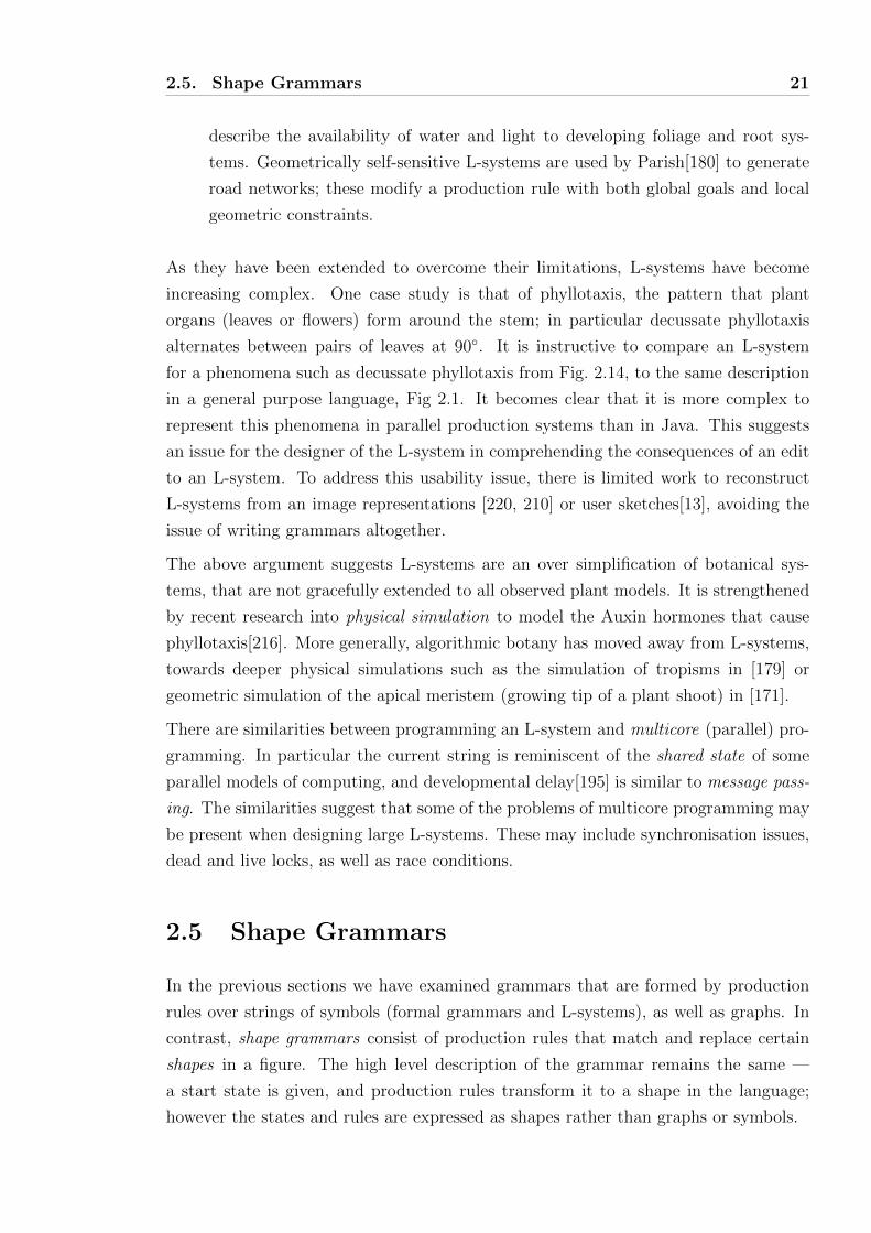
The formalism behind a shape grammar eventually[223] came to consist of a set of
shapes, S, a set of symbols, L, an initial labelled shape, γ0, and a set of production
rules, R; each production rules takes the form α→ β. The left hand side, α, specifies
zero or more labelled shapes, (S, L)∗, that are matched against the current shape. The
right hand side, β gives a labelled or unlabelled replacement, ∈ (S, L)+ ∪ S+. As
with the previous grammars, we begin with γ0, applying rules until all symbols have
been removed. At this point the current shape, γ is an element in the language defined
by the grammar.
In contrast to L-Systems, the production rules are not applied in parallel to all matching
instances, rather in a serial manner reminiscent of Chomsky grammars[41]. Given the
lack of restrictions on the context of the shape, we may see similarities to a type-0
Chomsky grammar.
An example of a very simple facade shape grammar is given in Fig. 2.15, left, using the
symbols L = N, T . We show the evaluation of one shape in the language in Fig. 2.15,
right, by repeated production rule application until no symbols remain. Various other
shapes in the language are shown in Fig. 2.16.
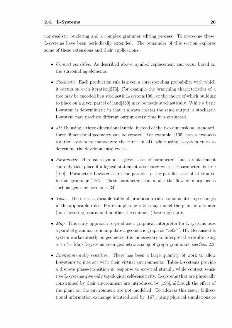
A single grammar production rule can often be matched to an infinite number of
positions on the current shape by matching subshapes. For example a rule containing
an arc may be positioned at an infinite number of points around a circle, as in Fig. 2.17.
Given this flexibility of rule application, it is a natural that the categorisation of the
different varieties of shape-grammars concerns itself with the mechanism for matching
α against the current shape, γ, the subshape problem. Common variations include:
• the shapes that may be matched — such as only lines, rectangles or curves in 2D
or 3D,
• the type of matching that occurs — whether only whole shapes (such as rectan-
gles), or subshapes (such as one corner of a rectangle), may also be matched. The
2.5. Shape Grammars 23
T
T
T
T
T
rule 1
rule 2
rule 3
rule 4
rule 5
rule 6
rule 7
rule 8
initial shape
TT T
TT T
T T
T T
T T
T T
rule 1
rule 2
rule 4
(2) rule 8
(2) rule 6
T
T
T
initial shape
T T
T
T
T
T
T
T
T
T
T
T
T
T
T
Figure 2.15: Left: We introduce a shape grammar consisting of 8 shape rules. Theshapes on the left of each arrow may be replaced by the shapes on the right of the samearrow. Right: An example derivation of this shape grammar that creates a bungalow.The number of applications of a rule are specified in parentheses.
Figure 2.16: Four evaluations of the shape grammar given in Fig. 2.15, with therules that created them.
2.5. Shape Grammars 24
A AAA
...
Figure 2.17: Left: A shape grammar production rule that positions a tree on anarc. Right: If we allow subshape matching under rotation we may position trees at aninfinite number of locations on a circle. We show the result of several applications ofthe production rule upon a circle.
(x2, y
2)
(x3,y 3
)
(x4 , y
4 )(x
5,y 5
)
(x1 , y
1 )
(x6 , y
6 )(x
7,y 7
)
(x10,y 10
)(x
8 , y8 )(x
9 , y9 )
(x2, y
2)
(x3,y 3
)
(x4 , y
4 )(x
5,y 5
)
(x1 , y
1 )
Figure 2.18: A single parametric shape grammar production rule inspired by[223].The accompanying schemata might specify that the new point (x6, y6) lies on the linebetween existing points (x1, y1) and (x2, y2), and similarly for the other new points.This parametrisation permits a language of nested pentagons to be defined.
advantage of subshape matching is that it allows more “emergent” (unexpected)
shapes to be generated,
• the transform we are allowed to apply to alpha to locate a match — such as
isometries, rigid transforms or affine transforms, and
• whether any parametrisation of α is allowed.
These parametric shape grammars [223] are variants which allow the arbitrary parametri-
sation of production rules. We show an example parametric rule in Fig. 2.18. There
are no computational limits placed on these rules, and are typically expressed in the
corpus by prose[222], or omitted entirely[72]. These parametrisations can be also used
to limit the repetition of rules, for example by adding area or height conditions.
The computational complexity of finding potential matches of α in the current shape,
γ, the subshape problem, is well studied. The matching of whole labelled shapes has
2.5. Shape Grammars 25
a linear computational complexity in the number of the current shapes. Therefore
there are well developed algorithms and systems for matching rectilinear[131, 130] and
curved 2D shapes. However parametric subshape recognition is NP-hard[279], even in
the case of a rectilinear shape vocabulary. This has not stopped implementations of
the parametric case in 2D[153]. The theory of shape recognition in 3D is addressed by
[132], against straight line figures only, while [37] introduces an implementation that
limits their use to circles and arcs. The issue of subshape matching with general curves
and surfaces in 3D is still unaddressed in the literature.
Despite these complexity issues, shape grammars have been widely applied in academia.
The initial examples were artistic drawings[227] and 2D architectural plans[225]. These
were extended to 3D isometric plans of houses, generated using parametric shape
grammars[128]. 3D shape grammars are less common, and tend to be simple, such as
modeling historic soft drink bottles[37]. A wide range of applications have been found
for shape grammars include modeling the morphospace of chair-backs[125], Harley
Davidson motorbikes[198], and coffee machines[3].
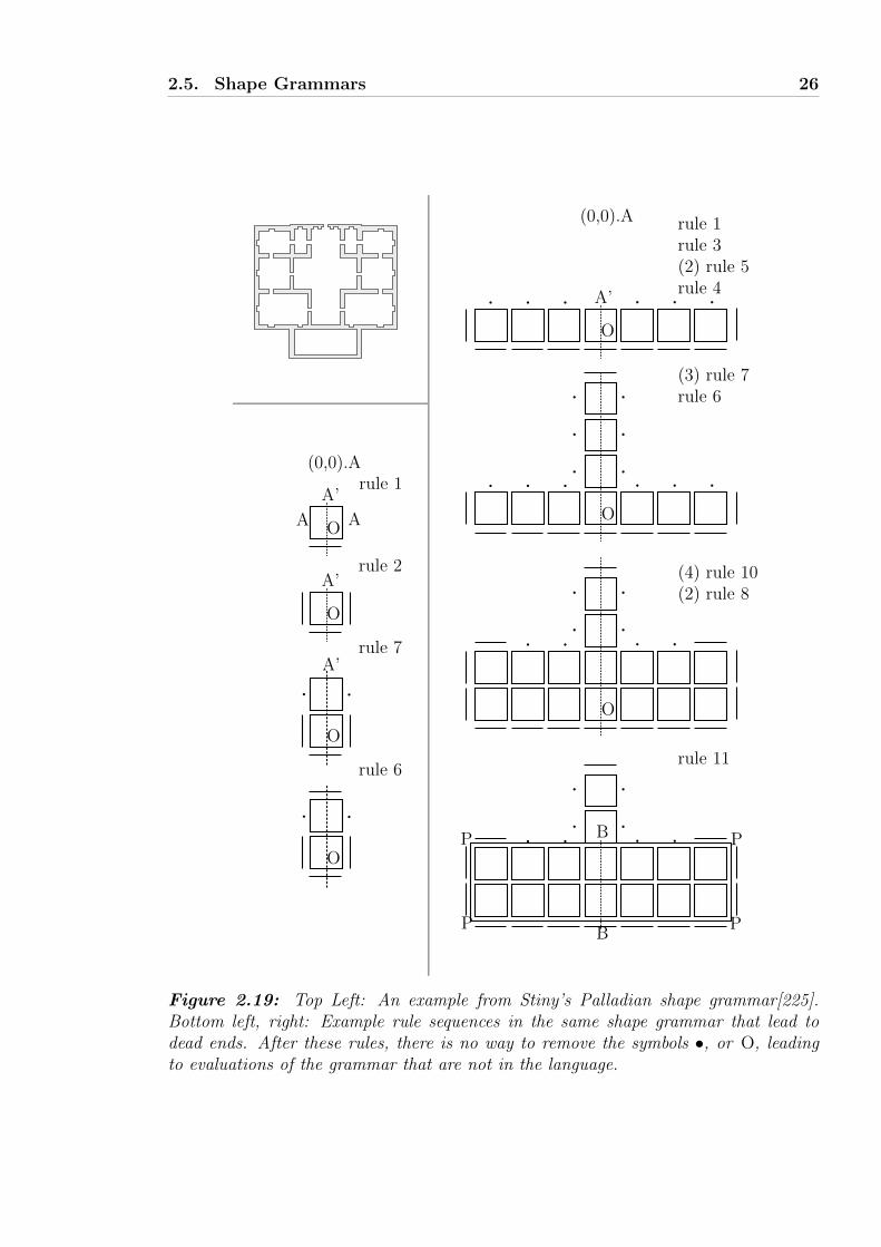
A subtlety of shape grammars are their termination criteria. The language specified
by the grammar does not contain all possible evaluations of rule sequences, but only
those shapes that do not contain symbols. There are sequences of production rule
applications in Stiny’s well cited Palladian grammar[225] that lead to dead-ends in
which the grammar can never terminate, Fig. 2.19. Of particular issue is the fact that
there are no guarantees as to how many times we might have to evaluate statements
in the grammar before a valid result in the language is generated.
The lack of a mechanism to specify situations in which a rule cannot be applied causes
additional difficulties with self intersection and termination (negative application con-
ditions in graph grammar terminology). A shape grammar rule with a β that is a
superset of the corresponding α gives rise to an infinite language. We present an exam-
ple in Fig. 2.16d, in which the facade may be indefinitely tall. This poses the problem
of how to stop a sequence like this from intersecting other geometry, especially in
non-parametric shape grammars.
Because of the requirement for shapes in the language to not contain symbols, and
the infinite nature of certain shape grammars, we may characterise shape grammars
as a search through some shape-space. The order of search can either be manually
defined (as in most of the corpus) or automated to produce figures automatically[89].
Regardless of the mechanism for choosing rules, sequences of rules will behave in one
of the following ways:
• All symbols will be removed, and a figure that the grammar describes will be
produced.
2.5. Shape Grammars 26
O
A’
A AO
(0,0).A
A’
O
A’
O
rule 1
rule 2
rule 7
rule 6
(0,0).A
A’
O
O
O
P B
P
P
PB
rule 11
rule 1rule 3(2) rule 5rule 4
(3) rule 7rule 6
(4) rule 10(2) rule 8
Figure 2.19: Top Left: An example from Stiny’s Palladian shape grammar[225].Bottom left, right: Example rule sequences in the same shape grammar that lead todead ends. After these rules, there is no way to remove the symbols •, or O, leadingto evaluations of the grammar that are not in the language.
2.6. Split Shape Grammars 27
• Symbols remain in the figure, but no further rules may be applied. The evaluation
stalls at this invalid shape (Fig.2.19).
• The evaluation continues endlessly. Either by force or choice the sequence of
applied rules is unending, and evaluation continues indefinitely. There are similar
situations in formal grammars, graph grammars and L-systems.
Other common issues surrounding the use of shape grammars are well summarised by
[84], for example
• the subshape and termination problems introduced above,
• the design of an adequate interface for the construction and application of shape
grammars,
• the lack of robust implementations for parametrised shape grammars,
• the difficulty in application to non-linear geometry, such as curved surfaces,
• the lack of a standardised shape-description, and finally,
• the lack of production grade or commercial systems for working with shape gram-
mars.
2.6 Split Shape Grammars
The computational complexity of classical shape grammars seems to have limited their
use to small scale academic projects. However in 2003, Wonka et al. created a spe-
cialisation of shape grammars, split shape grammars [269], with lower complexity. To
simplify their computation, these extend set grammars, initially within a 2D domain
of labelled nested shapes and using only whole-shape matching. These grammars have
been shown to be well suited to large urban environments, and facade generation in
particular.
As the name implies, a split shape grammar consists of production rules that take a
labelled shape and split it into a number of covering labelled shapes. Unlike a shape
grammar these labels are categorised as terminal or non-terminal. This delegation of
area to subsequent rules continues down a hierarchy until only shapes with terminal
symbols remain.
A principle assumption is that this hierarchical split operation is well suited to the gen-
eration of designed structures. There is ample justification for this assumption in the
2.6. Split Shape Grammars 28
literature of early urban modeling pipelines, such as the book A Pattern Language[9],
which introduces a hierarchy of 35 guidelines for the design of of urban areas, ranging
from “major city structures” and “common land” to “structure of the floor and walls”
and “furnishing”:
“The elements of this language are entities called patterns. Each pattern describes a
problem which occurs over and over again in our environment, and then describes the
core of the solution to that problem, in such a way that you can use this solution a
million times over without ever doing it the same way twice.”
The book is representative of the architectural literature in that it purports to present
solutions to urban design problems, without providing sufficient details for an compu-
tational implementation, for example:
“Pattern 10...Do this by means of collective regional policies which restrict the growth
of downtown areas so strongly that no one downtown can grow to serve more than
300,000 people.”
This hierarchical split approach to urban languages presented by A Pattern Language
is quite pervasive in the computer graphics literature, with examples such as [70], [97],
[11], and [180] using variations on the theme of a hierarchical urban decomposition.
Returning to Wonka’s 2003 paper[269], we observe that this concept of a strict hierarchy
in urban design is exploited to simplify shape grammars.
Compared to shape grammars, split shape grammars have the advantages of fast com-
putation and no dead-ends during the evaluation. The subshape problem is bypassed
by using a set grammar[224] in which matching takes place based on a whole shape and
a symbol. This removes the emergent behaviour of subshape matching, but permits
finding all possible shape matches in time linear to the size of the existing figure. While
certain split shape grammars may be evaluated endlessly, if they do terminate they are
guaranteed to supply a valid shape.
Muller et al.’s later influential paper, Procedural Modeling of Buildings [164], extends
the concept of a split shape grammar to 3D and introduces a written formalism for split
shape grammars, CGA Shape. The system has gained widespread use and notoriety as
it has been successfully commercialised[66].
A CGA Shape grammar consists of an initial labelled shape and a set of production
rules, each with a certain priority. All the applicable rules with the highest priority
are executed before others; this priority mechanism is exploited to produce differing
2.6. Split Shape Grammars 29
y
x
y
x
z
3: hex Subdiv(“x”,1r,1r,1r){A|A|A}
2: hex Comp(“sidefaces”) {A}
1: hex T(1,0,0)S(0.4, 0.5, 0.5)I(“hex”)
Figure 2.20: The current scope in a CGA Shape grammar defines a frame and extentfor the production rules. Given the initial 3D scope, shown in the top left, and the initialgeometry, top middle, we show the result of three production rules. Rule one translatesand scales the frame before adding another hexagonal prism of dimension specified bythe transformed frame. Rule two performs a component split, creating 2D faces, givingthem each their own 2D frame. Rule three subdivides the current shape along the x axisinto 3 equally high prisms, and matching scopes.
geometry based on the required level of detail. Models with higher details are generated
by executing rules with lower priority.
To define the reference frame for the production of geometry, a scope is introduced
that defines a frame, as well as an extent, as in Figure 2.20. This is reminiscent of
an L-system’s turtle. When geometry is created, the scope defines the size, location
and orientation. When the current shape is split, the scope defines the orientation and
number of splits.
A production rule of a given priority in CGA Shape consists of a unique ID, a parametric
symbol to match on, an optional condition, a labelled successor shape that is generated,
and a probability with which the rule will be applied: id: predecessor : cond
successor : prob. The successor operation has an involved syntax that is able to
manipulate the scope via transforms, splits, repeats and dimension reduction. A 2D
example is given in Fig. 2.21. The condition is used to limit the applicability of the
rule, for example to shapes of a certain size, or if certain occlusion conditions are met.
These occlusion queries form a domain-specific environmental sensitivity that is used,
for example, to stop the production of windows occluded by roof geometry. This is the
only context sensitivity available in the system.
Split shape grammars have been successfully applied to the reconstruction of several
historical sites such as Mayan ruins[168], the ancient Roman city of Pompeii[163, 58]
2.6. Split Shape Grammars 30
facade
u
u
l
a
w w w w
w w w w
w d w w
wtwm
wb
dmdt
wl
wrwc
dldc
dr
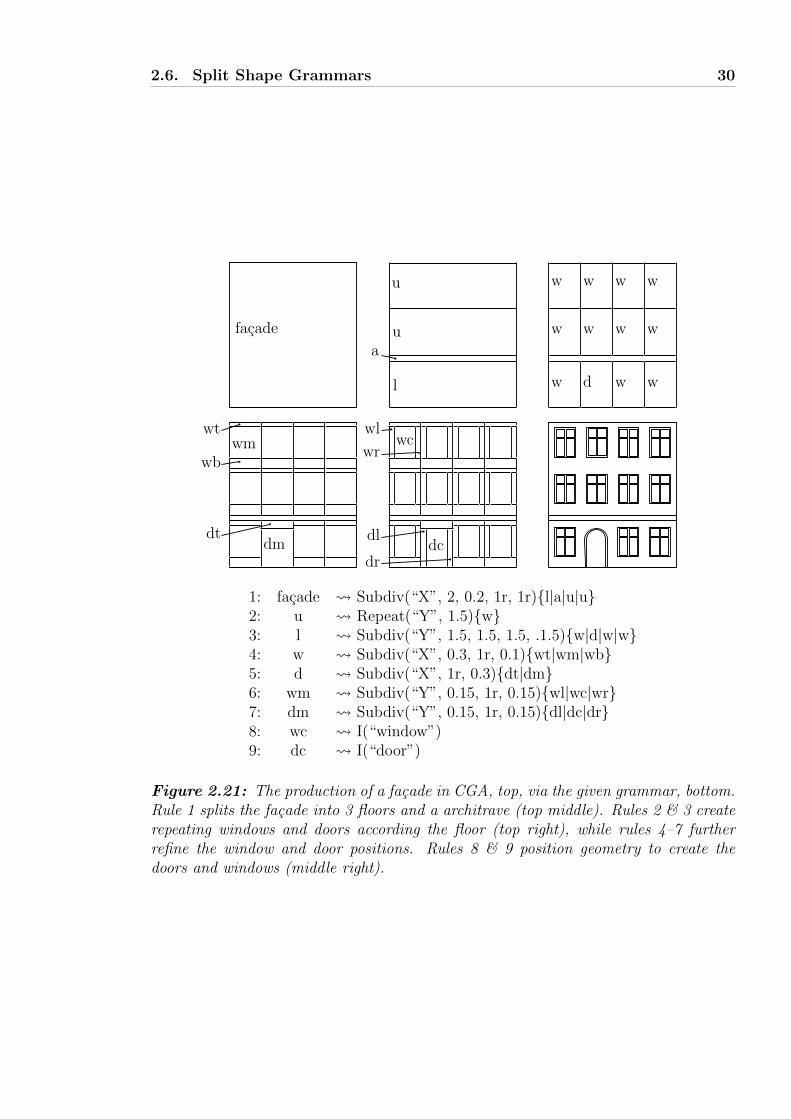
1: facade Subdiv(“X”, 2, 0.2, 1r, 1r){l|a|u|u}2: u Repeat(“Y”, 1.5){w}3: l Subdiv(“Y”, 1.5, 1.5, 1.5, .1.5){w|d|w|w}4: w Subdiv(“X”, 0.3, 1r, 0.1){wt|wm|wb}5: d Subdiv(“X”, 1r, 0.3){dt|dm}6: wm Subdiv(“Y”, 0.15, 1r, 0.15){wl|wc|wr}7: dm Subdiv(“Y”, 0.15, 1r, 0.15){dl|dc|dr}8: wc I(“window”)9: dc I(“door”)
Figure 2.21: The production of a facade in CGA, top, via the given grammar, bottom.Rule 1 splits the facade into 3 floors and a architrave (top middle). Rules 2 & 3 createrepeating windows and doors according the floor (top right), while rules 4–7 furtherrefine the window and door positions. Rules 8 & 9 position geometry to create thedoors and windows (middle right).
2.6. Split Shape Grammars 31
Figure 2.22: The instance locators of Lipp et al. [144] identify a component by itsposition in a derivation tree (left). After each production rule the index referred to(dashed lines) can be stored relative to the start, middle or end of the split sequence.The instance locator can be used to store modification to a procedural object, such as amodification to the style of a window, right.
and Malay houses[206]. Novel uses of split shape grammars include the presenta-
tion of uncertainty in archaeological findings by presenting several derivations of a
grammar[96], and animatable articulated objects structures[112].
Writing the production rules for split grammars is somewhat involved and required
specialist knowledge. Several attempts have been made to simplify the process. The
first presents the production rules as a graph[183], giving an understanding of the
relationship between application possibilities of the rules. However using this system
requires the user to comprehend the underlying grammar before using it. An alternative
is given by Lipp et al.[144], who allows the user to construct a grammar by editing an
example instance. By constraining the modeling tools to those that may be translated
to production rules, the user is able to quickly produce a PGM without interacting
with the grammar itself. When a user edits a single feature in an example instance,
this edit must be encoded into the grammar, in a persistent manner. To do this Lipp
introduces instance locators to store user edits in a split shape grammar, Fig 2.22.
Strict hierarchy and over-compartmentalisation can cause problems when working with
shape grammars[107]. For example sharing information about the number of elements
in a facade, as in Fig. 2.23, left. Additional difficulties are caused by problems placing
objects over two or more disjoint portions of the hierarchy, as in Fig. 2.23, right. In
these situations it is necessary to re-write the grammar to add a new shape, or to
add some portion of the shape to two separate portions of the hierarchy. Recently
work has begun to address this issue by creating connection patterns between portions
of two different shape grammars[129]. The problem of over-compartmentalisation is
uniquely critical to split shape grammars; while some shape grammars do use such a
hierarchy[225], many do not[146, 128].
2.7. Data Flow Programming 32
Figure 2.23: Left: The strict hierarchy may cause problems for coordinating features,as in this evaluation of the grammar of Fig. 2.21, showing a lack of synchronisationbetween the ground floor and upper windows. Right: The over-compartmentalisationmeans that it is impossible to place some features that cross over the hierarchy’s bounds,such as positioning an intercom near the door (black rectangle).
2.7 Data Flow Programming
Data-flow graphs are a model of parallel computation introduced as an alternative to
the classical von Neumann model.
Written imperative programming languages are typically a 1D sequence of symbols
which explicitly sequence instructions. This ordering of instructions is typically asso-
ciated with the von Neumann model, which executes a single instruction at a time. In
contrast, a parallel model of computation may execute many instructions concurrently.
To schedule the execution of a single instruction, a general requirement is that the
instruction’s inputs are available — whether they have been entered by the user or
calculated by a previous instruction. The necessity of the inputs’ availability creates
a dependence of the following instruction on the previous instructions’ execution, and
may be represented as a data flow from the previous function to the next, as in Fig. 2.24.
In this way data flow languages are declarative, allowing the executing system’s sched-
uler to determine the order of operations given the data flow constraints.
We introduce data flow languages, and in particular graphical data flow languages for
geometry as a typical example of a general non-written PGM system, before looking
at an example commercial application. The topic of data flow programming occupies a
wide range of our procedural spectrum. A data flow language with loops may be Turing
complete, and has many applications from parallel programming to task scheduling.
However there are a number of implementations that are graphical and geometrical —
their user interface is a graphical graph editor, and their output is geometrical. These
are the use cases that are of most interest to PGM, being of similar generality to shape
grammars, being concerned with the graphical domain.
2.7. Data Flow Programming 33
a b c d
mul mul
add
1 2
3
Figure 2.24: A data flow graph that calculates ab+cd given the mathematical conven-tion that multiplication instructions are performed before addition. The circular nodesare instructions, while the directed edges are the data flows. An inbound edge is an in-put to the instruction, while an outbound edge is a use of the output. Each instructionrequires that all of their inputs be present before calculating an output. For exampleinstruction 3 requires both instruction 1 and instruction 2 to be complete. However theorder of the operations are not specified in a data flow graph, so the execution ordermay be 123, 213 or instruction 1 and 2 may be executed in parallel before 3.
There are several varieties of data-flow graphs in the literature, we shall briefly examine
the token based model of Dennis from [54], introduced in 1974. Fig. 2.25 shows an
example graph for generating nested rectangles, showing examples of splitting and
combining data flow arcs. A token based data flow model models the arcs in data flow
graphs as FIFO queues of tokens. Each token is associated with a value, in our example
this value is either a rectangle or a Boolean. When a node has a token available on
each of its inputs it removes these tokens from its input arcs, computes an output, and
adds a token representing this output to any output arcs. The FIFO queues may be
initialised with tokens before the system is executed (as Fig. 2.25e). Ensuring that the
correct sets of input tokens arrive at the front of the FIFO queues at the same time
is challenging for the user, as demonstrated by the involved select/distribute syntax
of our example. This sequencing issue is one that will occur frequently in data flow
graphs.
We note that the graph of Fig 2.25 can only be used for the generation of one figure
at a time because of loops, negating the advantages of parallelism. This is somewhat
mitigated by the use of tags[54, 259], in which each invocation of the graph uses tokens
with different tags, allowing the same instruction node to execute on different sets of
input concurrently.
An alternative data flow model offers a different way to mitigate the sequencing issue,
by removing loops from data flow graphs. The structural data flow model[47] models
arcs as arbitrary and possibly infinite data structures. As computations are completed,
2.7. Data Flow Programming 34
area > 3 shrink rect
distribute
display
input rect
tf
selectfalse
f
a
bc
de
f
t
gh
Figure 2.25: A token based data flow graph (left) that generates nested rectangles(right). The data flow graph takes an input rectangle (a), shrinks and positions it (b)or terminates if the area is less than a constant (c), otherwise the sequence repeats itself.The sequencing issue of whether to take a new input rectangle, or iterate on the existingis addressed by the select and distribute nodes. The select node (d) outputs either thenew input rectangle, or the result of a previous iteration, based on the horizontal input;it is initialised with a token of value false (e) to initially take a new input rectangle.The distribute node (f) sends the output of the shrunk rectangle to one of two locations,based on the result of the area test. It is either discarded (g), or output (h) and usedin a subsequent iteration via the select node (d).
2.7. Data Flow Programming 35
Figure 2.26: A visual data flow diagram used for controlling the temperature of avirtual water tank.
these data structures are updated, and their values used by subsequent nodes. Struc-
tural data flow diagrams do not require loops as the token based systems do, however
this comes at the cost of storage; all computed values are retained by the data struc-
tures. Additionally nodes must be equipped with the logic to comprehend the, possibly
involved, input data structures.
While textual systems, such as LAU[188] and CAJOLE[101], focused on parallelism
and efficiency, another early justification for data flow programming was ease of use.
Curiously the development of easy to use graphical user interfaces to data flow lan-
guages preceded these formal written languages. In particular Sutherland introduced a
data flow editor[230] in 1966, 8 years before Dennis’ work. This system used a light-pen
to edit the structure of data flow graphs, and define functions by drawing nodes and
arcs. There followed many graphical data flow research languages, with examples such
as the Graphical data-driven Programming Language[48] and Grunch[50], a graphical
interface to CAJOLE. Many of the graphical programs were more visually complex
than their textural counterparts. In particular embedding a data flow graph into the
plane often leads to the crossing (without connecting) of graph arcs, making reading
the graph quite difficult. However this did not stop the use of graphical data flow
languages in industry, with systems such as Prograph[152] for general programming
and LabVIEW[113] as a digital laboratory, Fig 2.26.
There are several interesting diversions at this point that are beyond the scope of this
chapter:
• Data flow graph editors cannot express anything more than a written language (at
their most expressive they are still only Turing complete) despite their additional
dimensions. However many authors make the claim that graphical programming
is easier as it is more difficult to introduce syntax errors than when writing text
based programs.
2.7. Data Flow Programming 36
Figure 2.27: A random walk (red line, top right) programmed in the Scratch visualprogramming language[200]. Statements are chosen from the palette on the left to beadded to the program in the centre. The execution of the program is performed by thecat sprite in a turtle-like manner, top right. Note that invalid expressions may not beprogrammed, for example there is no attachment point to add a further operation aftera “loop forever” statement.
• There are a significant number of graphical editors for imperative programming[234,
85]. These exploit the ease of use of graph-based systems to appeal to, for ex-
ample, those new to programming. For example Scratch[200] shown in Fig. 2.27
is able to create geometry. These control graphs describe the sequence of op-
erations, rather than the data dependencies, usually allowing side effects and
mutable data structures which data flow programming largely avoids.
• We may create graph based graphical visualisations of many aspects of a pro-
gram. For example the data structures may be modelled by the Unified Modeling
Language (UML) or we may animate the flow of data[209]. These are analytical,
not generative, applications of graphs to programming.
As graphical hardware advanced it became clear that the graphical editing of data flow
programs was a good candidate for creating geometric programs. To clarify, not only
is the program edited graphically, but also creates geometric output. These systems
provide a widely used example of PGM without written programs, albeit under another
name.
The Fabrik Programming Environment[149] allowed 2D graphics, user interfaces, and
their elements, such as scroll bars, to be constructed within a dataflow environment,
but suffered from “poor performance”. Conman[95] utilised data flow graphs on more
complex graphics hardware to create 3D objects. A user of the system could construct
nodes that interact with the user, allowing user interface sliders, 2D curve editors, and
arbitrary scripts to create 3D objects. Later Lovejoy et al. used the Prograph data
2.7. Data Flow Programming 37
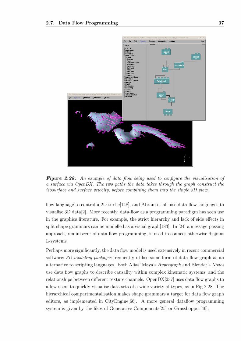
Figure 2.28: An example of data flow being used to configure the visualisation ofa surface via OpenDX. The two paths the data takes through the graph construct theisosurface and surface velocity, before combining them into the single 3D view.
flow language to control a 2D turtle[148], and Abram et al. use data flow languages to
visualise 3D data[2]. More recently, data-flow as a programming paradigm has seen use
in the graphics literature. For example, the strict hierarchy and lack of side effects in
split shape grammars can be modelled as a visual graph[183]. In [24] a message-passing
approach, reminiscent of data-flow programming, is used to connect otherwise disjoint
L-systems.
Perhaps more significantly, the data flow model is used extensively in recent commercial
software; 3D modeling packages frequently utilise some form of data flow graph as an
alternative to scripting languages. Both Alias’ Maya’s Hypergraph and Blender’s Nodes
use data flow graphs to describe causality within complex kinematic systems, and the
relationships between different texture channels. OpenDX[237] uses data flow graphs to
allow users to quickly visualise data sets of a wide variety of types, as in Fig 2.28. The
hierarchical compartmentalisation makes shape grammars a target for data flow graph
editors, as implemented in CityEngine[66]. A more general dataflow programming
system is given by the likes of Generative Components[25] or Grasshopper[46].
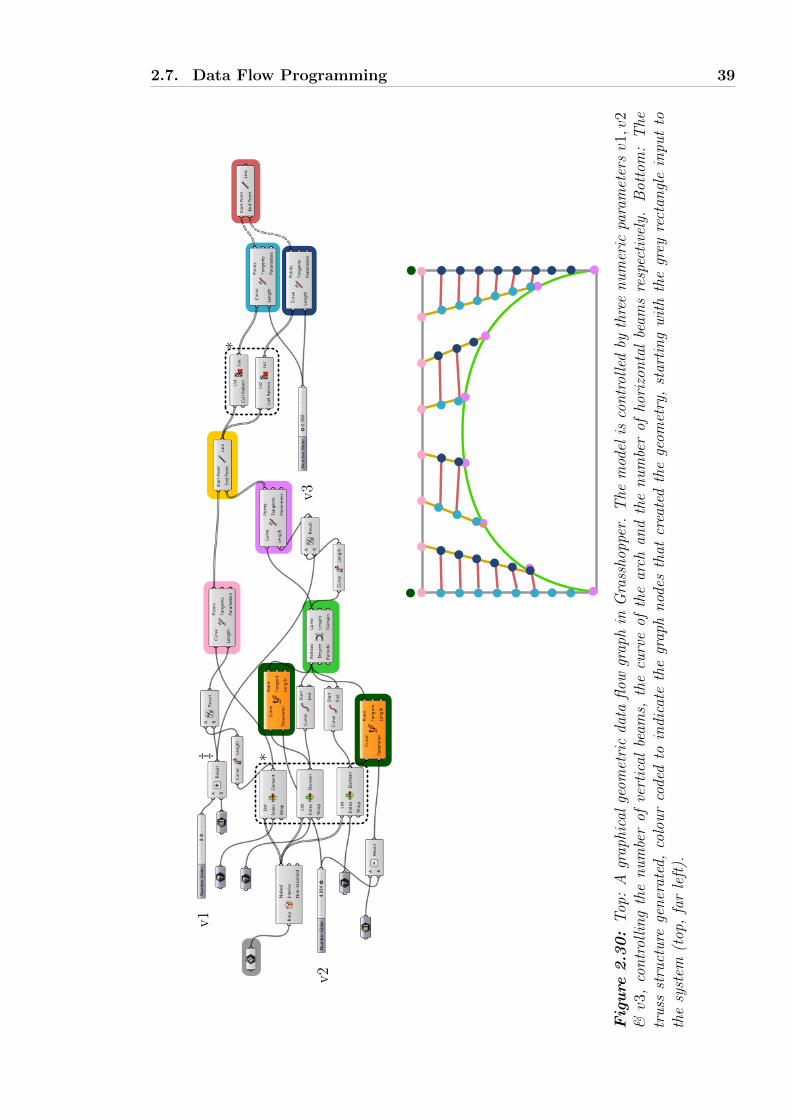
2.7. Data Flow Programming 38
v3v2v1
Figure 2.29: The result of varying the parameters v1, v2 & v3 in the Grasshopperparametric model of Fig. 2.30.
To conclude this discussion of data flow graphs we introduce details of Grasshopper to
give an indication of the typical tools available in these languages. Grasshopper uses a
structural data flow graph to describe procedural geometry. We give an example of a
Grasshopper data flow graph in Fig 2.30, to create the geometry of a procedural truss
bridge in Fig 2.29.
The structures transmitted along the arcs are nested lists, each nested to a depth
specified at compile time. Because only lists with the same nesting depth can be used
as inputs to the same function, Grasshopper’s UI indicates the nesting depth by the
type of line between nodes (undecorated, double or dashed lines for single elements,
lists-of-elements or lists-of-lists-of-elements respectively), as in Fig 2.30. To address
the sequencing issue, when an operation node takes more than one input Grasshopper
specifies several data-matching techniques, demonstrated in Fig. 2.31, based on the
number of evaluations of the operation — either the shortest, longest, or product of
the sizes of the inner most list. In addition there are a number of operations for
re-ordering or selecting elements from the data structure, marked by ∗ in Fig. 2.30.
However they are only able to manipulate elements in the inner-most list; more complex
patterns require writing programs to order the nested lists.
As an aside we note that data flow programming in no way alleviates the standard
numerical computation issues, as witnessed by the removal of a small delta in two
places of the computation, marked ‡ in Fig. 2.30.
2.7. Data Flow Programming 39
*
*
‡v1
v2
v3
Figure
2.30:
Top
:A
grap
hica
lge
omet
ric
data
flow
grap
hin
Gra
ssho
pper
.T
hem
odel
isco
ntr
olle
dby
thre
en
um
eric
para
met
ersv1,v2
&v3,
con
trol
lin
gth
en
um
ber
ofve
rtic
albe
ams,
the
curv
eof
the
arch
and
the
nu
mbe
rof
hori
zon
tal
beam
sre
spec
tive
ly.
Bot
tom
:T
hetr
uss
stru
ctu
rege
ner
ated
,co
lou
rco
ded
toin
dica
teth
egr
aph
nod
esth
atcr
eate
dth
ege
omet
ry,
star
tin
gw
ith
the
grey
rect
angl
ein
put
toth
esy
stem
(top
,fa
rle
ft).
2.8. Simulation Approaches 40
Figure 2.31: Data matching in Grasshopper. When joining the horizontal trussmembers, three techniques are offered — Left to right: Shortest list, longest list andcross reference.
2.8 Simulation Approaches
Creating grammars to describe man made objects is somewhat natural, as we are able to
encode the design process that a human may go through to create an object. However
there are many non-designed artifacts that we may wish to model in a procedural
manner, for example terrains, the historical growth of cities or damage to trees and
plants. Simulation approaches to procedural modeling involve the imitation of observed
processes to approximate the interactions within a model, and between the model and
its environment.
Simulation is used in a wide variety of ways to create geometry; we have already
seen examples of grammars simulating the growth of plants using L-systems[51] and
complex systems via data flow graphs[113]. We might even consider that searching
through grammar derivations is a simulation of the human design process. This section
explores a collection of systems that have simulation in common.
A very simple form of simulation are cellular automata; a specific example is provided
by Conway’s Game of Life[80] in which every simulation step updates a 2D array of
cells (boolean values) using very simple rules. As illustrated in Fig. 2.32, these simple
rules are executed in parallel on every update step, possibly changing the value of a
cell. Despite the simplicity of the rules, different starting values for the cell yields a
wide range of persistent and varied forms.
Attempting to program Conway’s Game of Life for a particular purpose is often quite
involved, however it delights in the unexpected behaviours that may be observed as
the simulation progresses. These unexpected or emergent behaviours have been better
studied in simpler still automata, such as those 1D systems studied by Wolfram[267].
Fig. 2.33 shows certain very simple rules creating complex patterns. There are 256
similar sets of rules, and this example is one of two examples that exhibit these emergent
Emergent behaviour seems to be very powerful as it produces intricate patterns from
2.8. Simulation Approaches 41
0-12-34-8
prev
ious
neighb
ours
next
0-234-8
n=0
n=10 n=200
Figure 2.32: Left: Conway’s Game of Life[80] simulation takes place on a 2D grid,the transition from a living (black) to a dead (white) state occurs based on the currentstate and the eight neighbours (top). Middle: The glider pattern, which self-propagatesalong a diagonal as the simulation progresses. Right: A space-filling pattern by HartmutHolzwart, at simulation steps 0, 10 and 200.
. . .
Figure 2.33: A Wolfram cellular automata defines a transition over a 1D sequenceof cells who are either alive (black), or dead (white). Left: In this particular case “rule30” specifies these eight transitions given a context of three cells (the cell to the left,the cell itself and the cell to the right). Middle: When applied in parallel these rulesmutate a start state consisting of a single black cell in a deterministic manner. Right:We may repeat this procedure a large number of times to generate an complex emergentsystem of local structures throughout the right hand side of the pyramid.
2.8. Simulation Approaches 42
very concise descriptions. For these reasons simulation seems to lie on a cusp on
our spectrum of procedural modeling. Those general models that we have already
examined, may exhibit emergent behaviour, while those that follow are less likely to.
However, by definition, emergent behaviours are not intended. It is difficult to engineer
these system with particular properties; perhaps the only way of working with these
systems is to have a large library with known behaviours, and to select the system with
the most desirable properties.
Turing’s work on emergent patterns in physically based simulations[244] suggests that
this library approach may be the one favoured by natural selection; appropriating
emergent patterns into situations where they are evolutionary advantageous. However
these approaches have not found much traction in the computer graphics and procedu-
ral modeling mainstream. Examples are limited to corpora to texture synthesis [154]
and the physical simulation of plants. Smith et al. construct a time-based 3D growth
simulation of the meristem (growing tip of a plant’s shoot) in [216]. By modeling the
flow of growth hormone auxin through this region, and the geometric changes that
it produces, the model produces a realistic geometry demonstrating several modes of
Phyllotaxis.
As well as simulating the processes within a plant, there is also a body of work that
simulates the environment surrounding a plant. 3D (voxel) cellular automata may
be used to model the intersection, proximity and occlusion of a plant[90]. Traumatic
events, such as branches breaking may be modeled as step events during the simulated
growth of a plant[51]. The growth of a tree through a volume can be simulated as
a space colonisation algorithm[205] while structural simulation can create balanced
trees[104]. Finally some systems simulate the interaction between both internal and
external factors; for example work by Prusinkiewicz et al. growth[167] simulates both
the plant-state, via L-systems, and exogenous factors such as the availability of daylight
and water.
Another frequently simulated domain are cities. Many systems exist for modeling land
use, populations and travel costs within cities[255, 212]. Mostly these use grids of data
points, or fixed-structure cells to represent design and layout, some even use cellular
automata to model these processes[8, 108].
The introduction of PGM to urban modeling simulations has allowed the creations of
detailed visualisations of the resulting cityscapes that change over time. Typically geo-
metric city simulations follow the same procedural urban modeling “waterfall” pipeline
as time-static procedural cities[180], an example of which is given in Fig. 2.34. Major
roads, such as motorways and A-roads provide access to a quarter, an area with partic-
ular characteristics. Access within the quarter is provided by minor B-roads. The area
2.8. Simulation Approaches 43
Major Roads
Quarters
Minor Roads
Blocks
Parcels
Mass Models
Facades
Figure 2.34: A typical urban modeling pipeline, similar to [260] and [250].
between B-roads becomes blocks, which are further split into parcels of land. Finally
buildings are positioned on the lots — the 3D geometry described by mass models, each
face of which is then assigned a facade. When working with discrete time-step simula-
tions, as in the 2D model by Vanegas et al.[249] or 3D model by Weber et al.[260], it
is necessary to repeat this course to fine hierarchy with every time step. Examples of
Weber’s resulting land-use and transport map are given in Fig. 2.35.
This concept of a single pipeline is a gross simplification of the processes that occur
within a real city, in which many other factors are considered — for example major
roads must take into account and avoid historical buildings. However the waterfall
pipeline is a computationally efficient system with proven results. A system that al-
lows for interactive feedback between users of the simulation and the system itself is
presented by Vanegas et al.[251]. The user may edit values in the simulation using
a paintbrush tool, after which the simulation then commences and the system brings
the underlying behavioural and urban models back into equilibrium under the new
assumptions. This is a useful urban planning tool for quickly examining the results of
decisions, such as building new roads in neighbourhoods.
A further use for simulation at the building level is for the investigation of the physical
strength of a system. For example we may wish to:
• identify the safe range of parameters in a parametric model, such that our building
is able to support itself[264].
• design a truss structures to support certain loads[215].
• find self-supporting free-form surfaces[254] that are sufficiently strong to be con-
structed.
• build furniture that is both stable and durable[246].
Each of these systems allow the user to specify a model and then simulation is used
to search for physically stable variation. This approach blends artistic human design
elements with automated reasoning about the properties of such a design.
Finally we find systems that use simulation for interior design. Two recent systems at-
tempt to position a given set of furniture in room by maximising an evaluation function.
Merrel et al.[158] encode various interior design guidelines, such as the distance chairs
should be from one another to permit conversation. Starting from a user suggestion,
the system is able to find a solution that accommodates these guidelines. Alternately
Yu et al.[278] learn pairwise relationships between items of furniture from several exam-
ples, and include occlusion constraints to ensure clear paths between doorways. Both
of these systems simulate a walk through an evaluation function by Markov Chain
Monte-Carlo sampling. While this is perhaps not simulation in the classical sense, it
may be seen as simulating a human designer’s exploration of the design decisions.
2.9 Inverse Procedural Modeling
As we have seen, the creation of procedural models is quite involved, requiring consid-
erable knowledge of grammars and languages. Recently there have been attempts to
generate procedural models from real world examples, the process of inverse procedu-
ral modeling. As with much of the shape grammar literature, the focus has been on
applications to the urban environment.
The data from the input examples may have been captured via multiple cameras and
terrestrial or aerial LiDAR (LIght Detection And Ranging, Sec. 2.12 contains further
2.9. Inverse Procedural Modeling 45
details); therefore it may contain significant quantities of noise. Identifying features in
this data is the first challenge, for urban environments in particular repeated features
are of significant importance. Recent techniques[159, 184] for identifying such fea-
tures in noisy data cluster the transforms between similar local features to determine
prevalent transforms. To reduce noise in the input data, RANSAC[71] is a popular
algorithm, and is utilised by GlobFit[138] to clean meshes making assumptions about
features such as planar surfaces, repeated distances and shared angles. Finally we can
form descriptions of 3D meshes as a tree of such patterns and symmetries[258] for
compression and error correction.
The grammar extraction techniques presented in this section mainly use the models
derived to compress data, rectify noisy captured data, or to extrapolate data to fill
holes. There has been relatively little work to re-target the extracted procedural models
to create novel geometry.
Before we examine systems that derive entire grammars themselves, we note that there
is a quantity of work on fitting parametric models to existing data. In the field of
urban layout reconstruction Aliaga et al.[12] learn descriptive parameters for a road
network via statistical analysis; this is then used to create new road maps. Alterna-
tively a template shape grammar may be parameterised to match input from vision
techniques[151].
The construction of grammars from examples has proved difficult, and the majority of
solutions rely on meta-heuristic techniques to search for a suitable candidate. Typically
these techniques repeatedly manipulate the grammar and compare the current results
with the noisy input data. In early work, Dick et al.[55] fit a grammar from several
images using a reversible jump Markov chain Monte-Carlo technique. The grammar
used is relatively simple — a set of walls formed the model, and each wall having a
set of associated decorations. The work is notable as it was able to reconstruct unseen
portions of buildings. Another system that uses a simple grammar and rjMCMC is
that of Ripperda et al.[202, 203] who utilise minimum description length of the derived
grammar as an evaluation criteria. By simplifying the grammar to an assignment
of a parameterised mass model to a number of quads covering the floor plan, [133]
successfully used rjMCMC to reconstruct large cities from aerial data.
More generally, rjMCMC has been recently used to force the derivation of an arbitrary
stochastic context free grammars to posses some specific qualities[232]; for example the
silhouette of a derived tree to some specified shape.
An alternative meta-heuristic for creating grammars are evolutionary algorithms. Si-
mon et al.[213] exploit a Pareto evolutionary algorithm to evolve a facade shape gram-
mar matching a number of images. In this system the appearance from multiple views,
2.10. Combinatory Modeling 46
and the depth correspondence form the evaluation (evolutionary fitness) function.
An incidental generation of grammars occurs in several places in the urban reconstruc-
tion literature. As [99] and [22] typify, the grammar complements the bottom-up land-
mark cluster analysis with a top-down grammatical description of the scene, enhancing
feature extraction. An alternative approach[239] is to only apply the bottom-up clus-
tering analysis, using the grammar to describe the properties derived from the input
data.
To avoid the need for meta-heuristics entirely Muller et al.[165] use the concept of
mutual information to identify repeating patterns in images of facades. The presence
of strong horizontal or vertical lines is used to determine the split-locations to generate
a CGA Shape grammar. This leads to a compact representation of the facade that can
be manually extrapolated to 3D. Another assumption that simplifies the construction
of grammars is that of a Manhattan World[248], in which all objects are orthogonal
polyhedra.
Muller’s automated extraction of facades is one example of using the extracted gram-
mars to re-target content. In this case the resulting facade could be re-sized arbitrarily.
Another example is Style Grammars [11]; a building grammar is created from 3D ge-
ometry, such that it may be retargetted to a different floorplan or height. This system
works principally by analysing the 1D patterns of sequences within a shape-grammar
like environment to predict a split rule for the resulting grammar. Finally Vstava et al.
extract L-systems from 2D vector designs by identifying similar components and then
analysing the transforms between them[220]. These L-systems may then be edited to
create unique new designs.
Inverse procedural modeling has the potential to create models that may be retargetted
to model novel situations, such as constructing buildings of different heights or floor
plans. However the results are, by design, derivative of the examples provided. For this
reason we may consider inverse procedural techniques to be more specific than general
purpose or simulation systems, yet more general than geometry capture or modeling
systems.
2.10 Combinatory Modeling
A subset of the inverse procedural modeling techniques that have an emphasis on
usability are combinatory modeling techniques. Combinatory modeling assembles sub-
components of example objects to create unique new geometries. These techniques fall
into one of three broad categories based on the level of input that the user is required
to supply.
2.10. Combinatory Modeling 47
Figure 2.36: Texture synthesis by the method of Wei et al.[261]. Left: An exampletree bark texture. Middle: The results of the synthesis. Synthesising a pyramid oftextures helps preserve large features. Right: Each pixel in a scan-line ordering of thenew texture is synthesised in turn. The feature vector of the red pixel is shown in thebottom right, This will be compared to the example texture to identify a suitable colourfor the pixel.
Combinatory modeling obtains its procedural element from the choices made during
automated assembly. When there is a choice of the choice of parts to attach, a range
of designs may result. However, whatever algorithm is used to make the derivation
choice, the result can only comprise subcomponents of the examples. For this reason
combinatory modeling is a very domain specific technique in our procedural spectrum.
Early work in combinatory modeling was inspired by the 2D case of synthesising tex-
tures. Given an example texture in the form of a bitmap, texture synthesis aims to
generate additional bitmaps that are at the same time characteristically similar to the
input and yet unique. As in Fig. 2.36, the standard technique is to grow an image
from an example texture by combining pixels from the example in a novel order, based
on their neighbourhood. To synthesise a certain pixel adjoining the patch, local pixels
from the patch form a feature vector. This is compared against all possible vectors in
the example texture to find the best match[59, 261].
Variations of texture synthesis include image quilting [60], which creates a reasonably
coherent grid of overlapping square texture tiles from the example texture. A minimum
error cut then determines the exact boundary through the overlapping pixels. An
alternative approach is to ensure that the tiles are always positioned in such a way
that adjacent borders do not contain discontinuities. An example of this approach is
Wang tiles[43].
When attempting the synthesis of 3D mesh-based geometry, local features, such as
those in texture synthesis, have been successful in reconstructing small missing patches
2.10. Combinatory Modeling 48
of meshes[208] using iterative refinement of nearest neighbour search and blending tech-
niques. The synthesis of entire objects has been attempted by tiling 3 space with com-
patible cuboids, with early examples using Wang Cubes [211]. Later examples by Mer-
rell et al.[156] use learnt adjacencies between neighbouring cuboids. Merrell extended
his work to arbitrary meshes[157], from which common adjacencies are extracted, and
a backtracking search constructs a new model consistent with these adjacencies. The
system is able to create a large quantity of architectural models with only a single
mesh as input, and no further user interactions. However the work with tiling geome-
try retains the limitation that only transformations allowed by the tiling, rather than
arbitrary transforms, are present in the output.
Domain specific tools use specialised techniques to relax this limitation and consider
non-local portions of the geometry when combining portions of meshes. Two notable
examples by Aliaga et al. synthesise city layouts, and facades. The first system[11]
extracts statistics about the roads and parcels in an example city layout and and uses
them to synthesise new portions of a city. The gaps between the roads are filled with
textured parcels generated using a Voronoi tessellation; the textures for these parcels
are taken from similar shapes from the example, and morphed to fit. Given a seg-
mented 3D facade the second system[11] decomposes it into a simple split grammar by
identifying 1D patterns, which can be retargetted to new geometry or floor plans. More
recently work has taken place to allow “intertwined” 1D sequences of elements over
such a facade, allowing for more irregular elements to be represented in a retargettable
fashion[140].
To overcome tiling limitations general symmetry analysis techniques have been devel-
oped [159] to identify compatible (symmetrical) subcomponents and valid location sites,
from an example model[30]. To address the subsequent issue of controlling which of
several subcomponents is positioned at a certain site, systems such as those by Kaloger-
akis et al. introduce a probability based approach[118] which learns the conditional
probability of certain classes of geometry being adjacent, and the spacial relationship
between the parts. To gather these probabilities, a large number of examples with
subcomponents are required, but the result is a realistic combination of those subcom-
ponents. For example when working with a corpus of aeroplanes, propellers are not
combined with jet-engined chassis.
In contrast to these unsupervised combinatory modeling techniques, interactive com-
binatory modeling of arbitrary meshes is addressed by Funkhouser et al.[75]. This
work introduces a tool-chain to allow the user to quickly create detailed models using
subcomponents from existing libraries. A shape-based search finds components in a
database, and both positioning and mesh blending tools are provided to the user to
align and attach those subcomponents to the existing model. This work is later ex-
tended to search for 2D sketched profiles of shapes in a library[135]. Other systems
specialise in the interactive synthesis by example of repeating 1D systems[176] and the
use of genetic programming to inspire the exploration of subcomponent-space[272].
An obvious limitation of combinatory approaches is that they are only capable of
imitating local and global patterns that have already been observed. While these
systems are very successful in combining geometry in new and interesting ways, they
are also limited by various geometric cases, where geometric continuity is required
between the subcomponents, as demonstrated in Fig. 2.37.
2.11 Shape Deformation
Moving towards more specific procedural modeling techniques we may decide to only
manipulate existing geometry, rather than attempting to design geometry from first
principles . Shape deformation is the continuous manipulation of an existing geometry.
Typically these models create a range of designs as they deform a shape, and so are a
more general procedural tool than geometry construction techniques.
Recent work has begun to explore the overlap between combinatory and shape defor-
mation techniques. Bokeloh et al. continued their work on identifying symmetry[29]
to exploit these repetitions to deform models, typically architectural, that contain du-
plicated elements. These repeats are often reminiscent of combinatory modeling tech-
niques. For example [30] resizes a repeating 1D sequence by repeating symmetrical
elements, either chosen randomly, or by a user. An alternative interface is given in [31]
which introduces sliding dockers as user positionable handles to deform meshes with
repeating elements. An underlying elastic deformation is combined with constraints
2.11. Shape Deformation 50
Figure 2.38: An example of the ‘morphing system of Beier and Neely[23]. Left: Twoimages (black) and their control points (pink, blue). Right: The result of a 50% warpbetween the two.
to preserve observed symmetries, such as straight lines or 1D repeating patterns. The
most recent system in Bekeloh’s series of papers [32] uses a linear system to maintain
basic relationships, after factoring out 1D or 2D repeating elements.
The first 2D image warping method was created by D. Smythe for the movie Wil-
low [217] in 1988; it was used to smoothly deform a goat into an ostrich, and finally
a tortoise. The user specifies the location of key points between the images by posi-
tioning a grid, and the system would create an image at a certain interval between the
examples, allowing the features to flow to different locations smoothly. To achieve this
effect the grid was smoothly interpolated between the two states, and the content of
the meshes blended. A similar technique was presented in 1992[23], that used discrete
handles instead of a grid, that weighs each pixel’s location relative to each handle. An
example is given in Fig. 2.38. A recent system by Igarashi et al. has a different goal; to
allow an image to be deformed as rigidly as possible[111]. This is applied to examples
to allow the interactive animation of images. A pair of linear solvers allow a mesh to
retain a physical rigidity, while being retargetted to a new shape. An alternative im-
age deformation technique is image resizing. Seam carving is a 2D technique to resize
images, whilst retaining the most important features[21]. By discarding low-energy
seams from an image, the most interesting features of an image can be retained, at the
cost of global distortions.
One of the earliest system to deform 3D objects was created by Sederberg[207]. This
scheme, analogous to the 2D system of Smithe, utilises a 3D lattice positioned over the
object to be deformed. By moving the points of this lattice, the geometry within can
be smoothly reshaped without introducing discontinuities. This technique is global, in
that the entire mesh is deformed when a lattice point is manipulated. Another global
technique[33] allows the user to position handles on the 3D mesh. After moving these
to a new location the system deforms the mesh such that it again touches the handles.
One issue with global deformations is that it is difficult for two physically local sections
of geometry to have different deformations without interference. For example, when
2.11. Shape Deformation 51
deforming the middle finger of a hand, it is likely that the index finger will also be
repositioned. A response to this was a local deformation — skeleton based deformation
techniques, in which portions of a 3D mesh are deformed in response to only a subset
of the skeleton. Different portions of the mesh are associated with different portions
of the skeleton, allowing for nearby verticies to be manipulated by entirely different
deformations. There are many different methods for defining a skeleton —
• In early work[136] the bones that comprise the skeleton are coordinate frames
defined by the user.
• Later systems[26, 277] use the medial axis of the mesh to define a skeleton as a
“shrunk” version of the mesh that can be animated and reconstructed.
• Lastly we may analyse a mesh to discover mechanical joints, and the joint limits
that may be present[273], to associate the correct portions of the skeleton with
the mesh.
One issue that is common to most deformation techniques, but skeleton based defor-
mation in particular, is the undesirable self-intersection of the mesh under aggressive
editing. Various approaches have been suggested to address this issue, including chang-
ing the weights near a sharp bend in the skeleton[136], or deforming the mesh based
on self-proximity[277].
Both the local and global techniques examined so far have been unable to identify and
preserve the symmetries and patterns present in man-made objects. To this end, there
have been several recent efforts to create tools specifically targeted to the deformation
of man-made objects. For example Cabral et al.[35] resize meshes using constraints
that specify that the angles must remain constant, and the edge lengths must remain
as similar to the original as possible. These linear systems can then be solved at
interactive rates to allow urban geometry to be resized by a number of user-placed
handles. iWires[77] instead analyse the geometry of the given object, to extract a
number of wire-like handles that can be used to deform the object. The analysis
reveals the symmetries between the wires visible in the shape, and these may then be
retained under user edits. Given a model that has a number of constraints, such as
orthogonality or planarity, Habbecke et al[93] present a method for deformation when
the user drags an arbitrary vertex. A combination of a linear model and compressed
sensing are used to ensure as few verticies as possible are moved.
Some mesh representations, such as planar quad (PQ) meshes, have underlying con-
straints on the location of verticies. PQ meshes require that all the faces of a mesh are
planar quads, and are useful when, for example, we wish to build curved glass roofs
2.12. Geometry Construction 52
from a patchwork of planar tiles. Yang et al[274] introduce a framework for deforming
such meshes by exploring a high dimensional space. This space is bounded by the
given constraints, and may be explored via 2D maps. The resulting mesh is found by
projecting back to 3D.
As a form of deformation parametric modeling is an often-overlooked subject in both
general academia and computer graphics[105]. Computer aided design (CAD) systems
are used to design 3D geometry in many industries. Typically these operate on similar
principles to geometrical modeling, but with the end goal of producing domain specific
results, such as AutoCAD[18] for standard-compliant architect’s plans, ArcGIS[17]
for maps, or Mastercam[218] for computer numerical controlled (CNC ) fabrication
machines. Parametric modeling is an extension to CAD to consider the design of
elements where parameters may vary, producing a range of objects, as in procedural
modeling. This offers a way for a draftsman to encode domain knowledge into a
model[14]; as they work the designer specifies which measurements are parametric,
and the constraints that are necessary for each measurement. As with PGM, there is
no standard format for parametric components[134].
An example of a deformation technique that is typically used to create a single in-
stance of a 3d mesh is digital sculpting. Commercial projects such as zBrush[187] and
Mudbox[20] provide the best example of this technique — users are able to manipulate
a 2.5D or 3D mesh by drawing strokes on the surface to mark the location of deforma-
tions. Typically users can push and pull the surface, as when sculpting a real-world
deformable material, such as clay. These tools are used widely by 3D mesh artists to
create highly detailed models, for example, reconstructing extinct animals from their
fossil remains[221].
2.12 Geometry Construction
Towards the most specific end of our procedural spectrum the systems we examine
do not create true procedural models, but only create a single geometric instance,
such as a 3D mesh. Typically every new geometric instance will require significant
human interaction. We begin our overview of this expansive subject by looking at
some examples of domain specific geometry modeling tools, then sample some geometry
capture methods, and finally examine 3D mesh construction techniques.
An overwhelming variety of domain specific geometric modeling tools are available.
Chen et al. exploit tensor field editing systems to design street networks in an urban
environment[38], exploiting the literature on the subject to build a novel urban geome-
try design tool. The Arches [185] framework presents a novel representation of terrains,
2.12. Geometry Construction 53
as well as sculpting and editing tools to manipulate the mass of of rocks, or introduce
features such as cracks. Another domain that has been approached is to allow the easy
modeling of flexible objects[257], by reducing the degrees of freedom that such objects
have in an intelligent manner.
Freeform architectural surfaces are characterised by large smooth curved areas, that are
not regular geometric structures. The work in graphics on these surfaces is largely con-
nected to modeling these surfaces as 3D meshes, with each face, having certain physical
properties. The faces are often constructed of planar glass sheets, often quadrilateral.
These surfaces are well represented by PQ meshes, but many mesh editing techniques
do not guarantee these planarity properties. One approach by Pottman et al. is to op-
timise a given thin PQ mesh such that each quad is within some planar tolerance[147],
another is to allow the user to explore the space of such meshes[274]. The generation
of thick, offset, surfaces to PQ meshes is studied in later work[190]. Instead of PQ
meshes, we may wish to construct our freeform surfaces from bendable strips of flexi-
ble material[192], or use such strips to create geodesic patterns[191]. These techniques
use elements of simulation to create one-time models, with a typical example being the
simulation of a cost function for the physical manufacture of the mesh faces[63]. The
authors present a cost function based on the reuse of face shapes and deviation from
the specified design.
A quantity of work aims to reconstruct 3D objects from 2D plans[275]. We may, for
example attempt to interpret 2D vector plans, typically created by CAD software, into
plausible 3D objects. Lewis et al.[137] introduce techniques to re-structure plans in such
a way as to make the data suitable for extrusion. However if we only possess a bitmap
image of the plan, without any of the meta-data associated with vector plans, a range
of machine vision techniques must be used to identify the different features[57]. These
techniques have also been used for rapid video-game environment construction[73].
Academic projects also explore sketch based deformation techniques, such as Keraut et
al.[123] who utilise shape from shading techniques to allow users to construct 3D meshes
from their 2D drawings of an object lit from several angles. More recent work allows
users to deform 3D meshes by sketching the position of highlights or silhouettes[83]. An
alternative to sketch based deformation, is the photo based approach of Xu et al.[271],
who use a photo to deform a 3D mesh to replicate the form of a certain 2D image.
This is achieved by decomposing the symmetry of the mesh and re-aligning it to the
silhouette given in the photograph.
Utilising 2D images to aid in 3D geometry synthesis forms an extensive sub-field of
geometry capture from sources such as single photographs, sets of photographs, LiDAR
and GPS data. In Sec. 2.9 we explored several systems that exploit a procedural
2.12. Geometry Construction 54
model as a reconstruction tool; there is considerable overlap between such systems and
the geometry reconstruction techniques given here that reconstruct a static 3D mesh.
A thorough treatment of this spectrum of reconstruction techniques is given in[166],
although we now give an overview.
Manual reconstruction from a single photograph is quite unconstrained and so relies
on domain specific information to produce useful results. Early attempts[109] required
further human assistance and exploited assumptions about objects always touching a
known floor to infer depth. More recent attempts exploit domain specific properties,
such as the strong rectilinear nature of facades[165], or the symmetrical nature of a
certain class of buildings[116] to automatically reconstruct geometry.
Given several photographs we may reconstruct a 3D point cloud over the surface of a
building, using techniques such as structure from motion[53]. To construct accurate
meshes from a low number of images, together with user interaction, one approach is
to use such 3D data as a mesh modeling aid. The Facade[52] system pioneered this
approach, using several images, with edges identified by the user, to reconstruct the
geometry from basic blocks. Another approach is given by Sinha et al.[214] who allow
the user to sketch polygonal faces that are then fitted to the recovered 3D point cloud
using the RANSAC algorithm. This is then followed by automated texture extraction
from the source images. A similar vision approach is used in [177] to reconstruct a
coarse 3D representation of a building site, such that the user can sketch the walls of
a building on embedded 2D planes.
To perform fully automatic reconstruction, we may make assumptions about the ge-
ometry in the scene. For example Werner et al.[263] assume an architectural scene
with a few principle edge directions. To automate reconstruction from general images,
generally a larger set of images are required. For example, an automated version of
the Facade system uses dense polygonal reconstruction from several photographs[189];
this is sufficient detail to reconstruct a coarse mesh of a single building. Larger scale
reconstructions require using hundreds or thousands of photographs to reconstruct ur-
ban areas in fine detail. Gathering sufficient data for these approaches is challenging,
with researchers using image-sharing websites[4], crowdsourced calibrated capture[115]
and novel games[242] to collect a sufficient number of images covering the geometry to
be reconstructed.
An alternative to optical photography is LiDAR reconstruction. LiDAR uses laser
range finding to plot a depth-map of some geometry. Common examples include street
level LiDAR for facade reconstruction[197], and aerial LiDAR for urban[280] or forest
environments[161].
The industry default 3D mesh creation techniques are mesh construction tools, these
2.12. Geometry Construction 55
a
b
c
d
e
f
g
h
ij
k
Figure 2.39: A slightly contrived mesh construction workflow to create a house (cen-tre). The walls, windows, door and roof are created using lofting, constructive solidgeometry, bevelling and manual modeling tools respectively.
have become ubiquitous, with commonly used commercial packages such as Maya[19],
Blender[74] and Sketchup[240]. In the most part this chapter has been discussing more
general alternatives to these techniques, however this tool chain is used to create the
majority of 3D geometry in use today.
A typical workflow to create a 3D mesh of a house in a is show in Fig 2.39. To create
the roof (Fig 2.39, ab), a user may manually add verticies (red points), and select
groups of verticies to form faces. Rotational, translational and scaling tools allow
these elements to positioned appropriately, (c). A door may be constructed using the
bevel tool. A cross section and path are defined (d) using manual modeling techniques;
an application of the bevel tool then sweeps the same cross section along the profile,
creating faces (ef). The loft tool is similar but takes a list of curves with the same
topology, but changing geometry (g) and creates solid faces between them (hi). The
loft tool creates the walls of the house, but to inset the windows we use constructive
solid geometry tools[238] to subtract the volume of a set of carefully positioned cuboids
(j) from the result of the loft operation (k). We note that there is no correct choice of
tool for each geometric element. For example manual vertex construction could have
been used for the entire mesh, or the walls could have been constructed via CSG over
an appropriate set of cuboids.
However a wide variety of research is still undertaken to create meshes, here we only
present a small sample. For example, given only a 2D sketch of a 3D object, recon-
struction is an under constrained problem; a problem that Structured Annotations [82]
approaches by asking the user to annotate a sketch to provide more constraints. Alter-
nately FiberMesh[172] approaches construction using a sketch-and reconstruct cycle.
A novel tool is the application of texture cloning to 3D to allow interactive mesh ge-
ometry copying from one mesh to another[231]. Finally Li et al.[139] address the issue
of the manipulation of irregular verticies in near-PQ meshes to achieve aesthetic or
structural benefits.
2.13 Digital Libraries
The most specific extreme of our spectrum of PGM contains libraries of objects. Given
the range of geometry creation systems available it should be not surprising that repos-
itories such as TurboSquid [243] contain upwards of 200,000 3D meshes.
Given such a variety of geometry, some search tools are required to allow users to locate
the geometry they require. Most of the commercial websites such as Trimble Ware-
house[241] or Turbosquid use text based search, an example result is show in Fig. 2.40.
However searching large collections of 3D meshes remains a active research area. The
seminal work in this area by Funkhouser et al.[76] indexes and retrieve meshes by
sketches or example models. The rotation invariant properties of spherical harmonics
are used to construct easily indexed feature vectors. An alternative feature descriptor
2.14. Summary 57
is given by [174], which uses the low frequencies of the depth map of the rendered
object. The rendering stage ensures the system is robust to irregular meshes, such as
those which contain holes. A different approach is to exploit the continuous variability
in a set of models to allow users to explore the set of models interactively, as in [175].
For example, users navigate from one airplane mesh to another by indicating that they
wish the wings to be further forwards on the fuselage. Recently fuzzy correspondences
have been introduced as a technique for exploring a library of meshes uses regions of
interest that the user specifies on an example model.
Because each model in the library has been manually created, they are free from many
of the artifacts that recovered geometry may contain. Furthermore they are free from
many technical concerns that come with many of the more general procedural systems,
such as termination criteria in the case of shape grammars. However, the user faces
several other issues in using this content — for example, given an existing lot in a
city finding a house of the correct style to fit, depends on the contents of the library.
Generating a large cityscape may require repeating objects from the library, or mixing
meshes of different styles and level of detail.
2.14 Summary
In general there are many axes on which we can classify the work on procedural mod-
eling, such as quantity of human interaction, or applicability to real-time situations.
However in this chapter we have introduced one such axis — a continuum of procedural
specialisation from the general purpose to the specific.
We have given examples examining the range of geometry that may be generated
with each system. From general purpose programming languages, that only happen
to be used for geometry creation, through complex grammar and inverse procedural
techniques, to simply finding the closest possible item of geometry in a library. Unfor-
tunately it is hard to make a quantitive argument about the trade off between power
and ease of use over this spectrum. This is due to the difficulty in capturing ease of use
information given the wide range of users’ abilities (both programming and artistic),
and in quantifying the range of results that a system can create. We may imagine
some future work in which users create a model with each system in the spectrum, and
we then evaluate the time it took the user, the fidelity, and the range of geometry the
created model creates.
Complicating matters we have observed an increasing number of cross over systems in
recent years — combining separate parts of this spectrum to increase the utility of the
system. For example,
2.15. Approach 58
• grammars are used in urban reconstruction via inverse modeling to more tightly
fit geometry.
• the 3D meshes created by tools can be positioned to form a facade using a shape
grammar, that itself is implemented in a general purpose programming language.
• simulation is used to evaluate the results of L-systems to create models of trees.
Given the broad range of geometry synthesis systems available today, users would be
well advised to find the most specific technique that has the required flexibility. For
example a video game artist may wish to “synthesise a large set of alien tower blocks”
with a shape grammar, a town planner may wish to “visualise this area of a city after a
10% increase in public transport usage” using simulation techniques, or residents may
only care to “visualise the new statue outside the town hall” using mesh construction
tools.
In our introduction we stated that in order to be useful, existing procedural systems
required users to write computer programs. With this spectrum of proceduralisation,
we can see a strong correlation between general, powerful systems and the requirement
to write computer programs. The most general geometry creation techniques, Sec. 2.1
to 2.7, require users to program. The type of programming involved was quite varied;
we have encountered systems that use a conventional language, a shape grammar, or a
data flow graph to specify an algorithm. Conversely, the the most specific techniques,
Sec. 2.8 to 2.13 do not require any programming. The user is able to generate a smaller
variety of geometry, often confined to a single domain. However they are able to create
models using a variety of easier to master techniques such as graphical editing (in the
case of shape deformation or geometry construction), discrete selection (in the case
of digital libraries or combinatory modeling approaches), or by selecting a number of
parameters (in the case of simulation systems).
If we start from the premise that we wish to build a system that is as general as possible
without writing a computer program in any form, we find the state-of-the-art in the
middle of such a spectrum.
2.15 Approach
We wish to possess a system that is as expressive as a split shape grammar, or data
flow programming system, but inspired by the types of user interface present in the
simulation or inverse procedural modeling approaches. Inspiration for a such a system
was forthcoming from Havemann’s thesis[105]. This provides some convincing examples
2.15. Approach 59
that an offset mechanism driven by the straight skeleton was a powerful accompaniment
to a written programming language. After studying a variety of man made objects
inside and outside an urban environment, it became clear that some generalised offset
mechanism could describe many features of man-made geometry.
The straight skeleton has a simulation-like definition, in which a 2D shape is shrunk
until it disappears, leaving behind it a subdivision of the original shape. The output is
promising because it was closely correlated to the input, and is quite predictable and
easy to understand via a user interface. However the skeleton also had some interesting
non-trivial outcomes, such as being able to split concave shapes into two, introducing
holes into faces, and leaving behind “arcs” which form part of the centrelines of a shape.
It is these emergent properties that we found we could exploit to create an expressive
range of geometry.
Chapter 3 introduces our detailed examination of the straight skeleton, the kind of
events that we observe as it shrinks, and the kind of degeneracies that occur if we
are unlucky. We continue to examine how the straight skeleton can be generalised so
that it becomes a more powerful modeling tool in more situations, whilst keeping its
desirable properties.
Given a theoretical understanding of the geometry, we continue to apply the skeleton
to the domain of urban procedural modeling. The urban domain has several prop-
erties which make it ideal for modeling with skeletons. Given the polygonal output
required for many tool-chains used to create 3D environments, the straight edges of
many architectural forms was appealing. Cityscapes also offer a more semantically and
geometrically demanding domain than, for example flora — facades have constraints
such as only locating doors at street level, and unlike procedurally generated botany,
the self-intersection of buildings is undesirable. Finally the urban landscape is well
documented, which facilitates easy to obtain reference material and comparisons.
Our first application of the straight skeleton to an urban domain was in identifying the
centerline of city blocks so that they could be split into lots. Existing systems assumed
a simpler model, in which the block was repeatedly split into two pieces, however
such a system was unable to represent the characteristic centrelines. In Chapter 4 we
examine a novel technique for the subdivision of city blocks using the straight skeleton.
The straight skeleton is combined with geometric construction techniques to give a
parameterised algorithm for city lot formation.
We continue into Chapter 5 to apply a generalisation of the straight skeleton to the
construction of solid buildings that may be located within such lots. The similarity
of the of the straight skeleton to a building’s roof is exploited and extended to gen-
erate a wide variety of interesting architectural forms. Repeated applications of the
2.15. Approach 60
skeleton are guided by user defined plans and profiles to generate buildings. The gen-
eralisations of the skeletons that we introduce prove to be robust building blocks for a
novel yet expressive system.The emergent properties of the skeleton gives very intricate
forms simple constructive definitions. These forms prove to be robust enough for large
scale cityscape generation, and capable of generating a wide variety of observed urban
structures.
61
Chapter 3
Various Skeletons
This section contains both literature survey and novel components. As introduced
in Interactive Architectural Modeling with Procedural Extrusions [121] I contribute
both the general intersection event and the mixed weighted straight skeleton. Fur-
ther contributions are the analysis of the weighted skeleton degeneracies, as “pub-
lished” in a blog post, and the description of the pincushion problem.
The straight skeleton is a geometric subdivision of a 2D shape, based on the notion of
“shrinking” the shape. In the following we will introduce the skeleton, its properties,
degenerate cases, computational complexity, and how to construct it. We extend the
standard definition of straight skeleton in several steps, introducing a hierarchy of
several skeletons, each of which is a generalisation of the previous. These generalisations
introduce additional degeneracies which we catalogue and suggest techniques to resolve.
Given the spectrum of geometry creation tools explored in Chapter 2, we were searching
for an expressive yet simple to use tool that would lie in the centre of our spectrum of
proceduralisation. It had to be general enough to create a width range of useful results,
but easily controllable without the need for specialist training. As we stumbled upon
the idea of offsetting geometry, and were introduced to existing results[105] relating to
the straight skeleton modeling the roofs of buildings, it became clear that the skeleton
had the potential of being a powerful modeling tool. The close relation between offsets
and the straight skeleton, introduced in Sec. 3.2 formed a powerful argument for this
particular geometric primitive having a wide range of modeling applications.
Discovering that the straight skeleton was also heavily used for roofs, we examined how
the skeleton could be extended to a larger domain. In the first case we noted that the
walls below a skeleton-created roof could be modelled either by an extrusion operation
3.1. Ways of Shrinking Polygons 62
or by the scaling the roof in the vertical direction until it became almost vertical. From
this point we explored the generalisation of per-edge slopes in the skeleton. Because
the definition of such a structure remained inherently simple and geometric the natural
user interface wasn’t programmatic, but instead visual.
In this chapter we examine the straight skeleton in detail and formally introduce a
hierarchy of skeletons, each of which takes the same basic information as input, but
expresses a wider range of geometric forms than the previous skeleton. In taking this
approach we can technical problems underlying the key skeleton concepts of offsetting,
or shrinking, a polygon.
3.1 Ways of Shrinking Polygons
There are many ways in which to shrink a polygon. Fig. 3.1 illustrates four published
techniques which translate shrinking edges in a self-parallel manner. These techniques
only vary in their treatment of reflex corners:
a) Given that each edge moves towards the inside of the polygon (green), parallel to
itself (white arrows), a multitude of techniques can be imagined by changing the
handling of the corners.
b) The medial axis [28]. A reflex vertex becomes a parabola as it shrinks, maintaining
a constant distance from the original polygon. The medial axis itself is a skeleton
defined as the set of all points within the polygon which are equidistant to two or
more points on the boundary of the polygon.
c) The straight skeleton[6] (SS), moves reflex verticies with the intersection of the two
adjacent edges. We investigate further properties of the straight skeleton in Sec. 3.2.
d) The linear axis [233] introduces hidden edges into reflex corners of the skeleton to
approximate the medial axis using only straight line segments. These hidden edges
immediately grow to “blunt” such verticies, reducing their “speed” as the polygon
shrinks.
e) A weighted variation of the straight skeleton (WSS ) was introduced by similarly
timed later papers by both Eppstein and Erickson [65], as well as Aicholzer and
Aurenhammer [7]. Both papers only give a passing mention to WSS and degenerate
cases are not introduced. The edges of the WSS are assigned independent speeds
for shrinking, which shall be examined further in Sec. 3.3.
3.2. The Straight Skeleton 63
a b c
d e
Figure 3.1: Techniques to shrink a polygon (a). These include the medial axis (b),straight skeleton (c), linear axis (d) and weighted straight skeleton (e). The result ofusing each technique to shrink the polygon by a small distance is shown (the light greenareas are lost to the shrinking process).
Our interest here is in the straight skeletons (SS and WSS), as these structures do not
introduce curved or additional edges, and, as demonstrated in Chapters 4 and 5, are
well suited to modeling certain classes of man-made objects as 3D meshes.
3.2 The Straight Skeleton
Let us consider the growth of a crystal, as in Fig. 3.2. As Aichholzer observed in [7], if
we were to watch such a crystal growing we would see that each face grows outwards
in a self-parallel manner, and the edge between two such faces moves outwards as the
intersection of these faces. Thijssen et al.[236] earlier explored the statistical properties
of such growth in crystals, introducing a 2D proxy for the original 3D geometry, Fig. 3.3.
This model of self-parallel growth is the reverse of the process that is performed to
calculate the straight skeleton, which is calculated by the shrinking of a polygon.
The straight skeleton (SS) is a 2d graph of arcs generated from this shrinking of a
polygon. Each of the edges of the polygon moves towards the interior at a constant
speed in a self-parallel manner. Occasionally the topology of the polygon changes as
we observe events such as an edge shrinking to zero length. As shown in Fig. 3.4, the
movement of the corners of the decaying polygon trace out the “skeleton” itself. These
arcs describe the path of the verticies as the polygon shrinks. Several examples are
3.2. The Straight Skeleton 64
Figure 3.2: Composite grey cubit crystals of galena with purple cubic crystals offluorite. Cave-in-rock, Hardin Co., Illinois, USA.
Figure 3.3: Given a set of square seeds (grey) on a line, the polycrystalline growthmoves outwards (green), and the movement of the corners traces out lines (blue).
3.2. The Straight Skeleton 65
Figure 3.4: Left: A shrinking polygon. Right: The arcs of the straight skeleton (blue)are formed by tracing the edges of the shrinking polygon.
shown in Fig. 3.5.
3.2.1 Constructing the Straight Skeleton
The SS is a graph of straight edges in R2. However we can interpret it as a terrain – a
set of faces in R3 which form a “landscape”[6], Fig. 3.6 right. This approach is taken
as it allows a comparison between the standard, unweighted straight skeleton, and
the various types of weighted straight skeletons (WSS), a generalisation introduced in
Sec. 3.3. The terrain constructed touches the polygon on each edge, and the projection
of the edges of the terrain onto the polygon forms the 2D straight skeleton.
The shrinking process is modeled as a sweep plane that rises with constant speed from
the input polygon, carrying with it the evolving shape. Each edge of the polygon moves
inwards with a constant speed relative to the sweep plane motion. The sweep plane
rises and the polygon shrinks, encountering various topological events. Eventually the
polygon shrinks to nothing and the skeleton is complete. The terrain approach allows
the events to be modelled as the intersection of three planes, rather than three 2D
edges, allowing the geometry of Chapter 5 to be constructed trivially.
To distinguish between the under constrained term “polygon” and a similar structure
with additional constraints, we introduce a plan, Fig. 3.6. A plan is a planar partition
(a straight line planar embedding of a planar graph) that divides the plane into finite
inside and infinite outside regions. A plan is a set of polygons consisting of corners
and edges, these are embedded in a plane parallel to the xy (“ground”) plane, so that
all corners of a plan have the same z (height) value. The jth polygon is described
by nj polygon corners cji ∈ R3 with 1 ≤ i ≤ nj. Each corner cji is connected to the
next corner (according to the polygon orientation) by an edge eji . The loops of edges
are oriented counter-clockwise, but polygons describing holes are oriented clockwise.
Additional bounded regions may be recursively located inside a hole. When discussing
3.2. The Straight Skeleton 66
Figure 3.5: A variety of polygons (green) and their straight skeletons (blue).
plans, indices are treated cyclically, so that in a polygon with corners cj1, cj2, and cj3,
the vertex cj4 means cj1.
Unlike the medial axis, there is no trivial description as to whether a particular point
within a polygon lies on the SS arcs. Instead, the skeleton is defined in the literature
as the result of the process of shrinking a polygon. That is, the only description of the
SS we have, is the algorithm for its construction.
To construct the skeleton, a sweep plane rises vertically from the input plan. This
sweep plane carries with it an active plan that defines cross sections of the terrain.
input plan
face
straight skeleton
arc
active plan
input-edge
corner
roof model
Figure 3.6: Straight skeleton terminology. The input plan defines the starting state ofthe construction, while the active plan defines the state part way through the shrinkingprocess. The final straight skeleton is a 2D graph consisting of arcs adjacent to faces.The roof model is an alternative 3D representation, the projection of which onto theground plane forms the 2D straight skeleton.
3.2. The Straight Skeleton 67
This 3D approach was first suggested by Eppstein et al. [65], although in spirit similar
to the original 2D proposal by Aichholzer[6], with data structures inspired by Felkel
and Obdrzalek[68]. However we use our own notation for continuity. The output of the
system is a series of skeleton faces that make up the 3D terrain. The edges between
the faces are named arcs after Aichholzer et al.[6], a term that we shall use in both 2D
and 3D interpretations of the skeleton.
As the SS is constructed, the sweep plane rises with constant speed, and the active
plan shrinks. In the case of the basic straight skeleton every plan edge moves with a
constant and uniform speed towards the interior of the polygon. As both the speed
of the sweep plane and plane edges are constant, each plan edge remains within the
same 3D plane. One of these direction planes is associated with, and intersects, every
edge in the input plan. As both the speed with which the sweep plane rises and the
movement of the edges is equal, the direction plane associated with each edge eji forms
an angle π/4 with the input plane. Each skeleton face lies in one of these direction
planes. To obtain a steeper or shallower roof from the SS we may scale the faces in the
Z direction appropriately.
At all times in this shrinking process we must ensure that the active plan remains well
formed. That is:
• The enclosed region remains to the left of every directed edge.
• No edge intersects another edge, with the exception of touching the neighbouring
edges only at shared corners.
• Every enclosed region has a positive, finite and non-zero area.
• There must be a finite number (zero or more) of such enclosed regions.
In the SS every active plan edge has the same constant, positive, speed. As the edges
move, the corners remain defined by the intersection of the adjacent direction planes
and the current sweep plane, as in the plans of Fig. 3.7. Therefore each corner in the
active plan, cji , moves between events with a constant, and often unique, speed and
slope relative to the input plan.
Fig. 3.8 shows that as sweep plane rises and the active plan shrinks, the plan may
become badly formed (red). To ensure that the active plan remains well formed, we
detect when more than two or more edges intersect and we make topological changes
to the active plan. We call these events ; as introduced by Aicholzer et al. [6] there are
two types of event:
3.2. The Straight Skeleton 68
x xx x
xx
Figure 3.7: As the active plan shrinks, the edges move with a constant speed. Severalplans (left, middle, right) are shown (green), along with their shape at a later time(grey lines). In a certain time, every edge moves the same distance (x), but movementof the corners is defined as the intersection of the corners and so the distance movedtypically varies. Very sharp reflex or acute angles between edges may cause cornersto move with high speed (right). This speed approaches infinite as the interior angleapproaches 2π from below, or 0 from above.
a
b
Figure 3.8: Left: the anti-clockwise oriented input plan. Middle: The active planat a split event (orange). Right: Without a split event, a portion of the active planbecomes badly formed. There are self-intersections at a and b, and the red region isdefined by a clockwise loop; that is, the edges define an infinite inside region outsidethe red area.
3.2. The Straight Skeleton 69
a
b
d
f
(adf)
(abc)
1.
2.
3.
(acd)
c
(def)
(acd)
e(def)
Figure 3.9: Left: the straight skeleton is given by arcs (blue lines) tracing the verticiesof a shrinking polygon (black lines). Each edge moves with a constant speed towardsthe interior of the polygon, and as it does the topology of the polygon changes in severaldifferent ways (dark green lines), during events. Right 1-3: The calculation of the SSis primarily a sequence of such events.
• Edge events occur as the length of an edge shrinks to zero. When a plan edge
shrinks to zero the direction planes defined by three consecutive (linked by cor-
ners) edges collide (Fig. 3.9, 2).
• Split events take place when two adjacent direction planes, and one non adjacent
direction plane collide (Fig. 3.9, 3). These split the region bounded by the active
plan into two parts.
.
We can describe these events in terms of the local plan around the direction plane
ac
a
b
c, d
db
before during after
Figure 3.10: Edge (a) and split (b) events that occur as a polygon shrinks. Peaks(c & d) comprise three co-sited edge events.
3.2. The Straight Skeleton 70
Figure 3.11: The active plan in two configurations in which intersection of unboundeddirection planes (intersection with active plan shown as red, cyan and orange lines) doesnot lead to an event as they occur outside the bounds of the associated edges.
intersection point, Fig. 3.10. Here we see the local active plan region before, during
and after edge events (a), split events (b) as well as peaks (c & d). As these peaks
may be considered to be three edge events occurring together, we classify them as edge
events.
Each of these events is witnessed by the intersection of three direction planes. However
not all intersections between three unbounded direction planes indicate an event. As
identified in Fig. 3.11, we must be sure that the faces intersect within the bounds of
the associated edges on the active plan. Also of interest to optimisation is that at least
one pair of adjacent plan-edges must be involved; an SS event consists of three edges,
at least two of which must be adjacent.
Every event creates one or more output arcs, a portion of the boundary of a terrain
face. Every arc is the boundary between two faces.
We present a crude algorithm in Fig. 3.14 that maintains this queue as new corners are
introduced by events. We defer describing the event handling in detail until Sec. 3.2.4,
noting that Felkel [68] simply gives a terse set of manipulations to the data structure
in the case of edge or split events.
The active plan is stored in a data structure that holds the corners of each polygon in
a doubly linked list, as illustrated in Fig. 3.12. There is such a list for every polygon
and associated holes. Each corner, therefore, has a pointer to its next and previous
corners (assuming counterclockwise order), as well as a pointer to its previous and next
direction planes. The corner is a point in R3 at the lowest intersection of the adjacent
plan edges. We may find the position of a corner in the active plan by intersecting the
corner’s next and previous direction planes with the sweep plane. Correspondingly,
an edge on the active plan is given by the positions of two consecutive corners in the
linked list. In this manner the linked list implicitly stores the active plan at the sweep
3.2. The Straight Skeleton 71
Figure 3.12: Left: The initial set of corners (yellow circles) and points in the doublylinked list (yellow arrows) that make up the input plan. Not shown are the pointersto the adjacent direction planes. Centre: As the sweep plane rises, and various eventsoccur the active plan may split. Corners are added and removed from the linked lists.Here two linked lists store an active plan with two polygons (yellow, purple lists). Right:By projecting the intersection of the corner’s direction planes onto the sweep plan, westore the implicit active plan (purple, yellow polygons)
Figure 3.13: Left: After all events have been processed, every arc is associated withtwo input plan edges. Middle: A single input plan edge has a set of edges, which maybe traversed (right) in a counter clockwise direction to construct a face (right, orange).
plane, via corners at or below the plane.
To simulate the rising sweep plane approaching events, a priority queue ordered by
height (z) is kept, specifying triplets of edges colliding at a certain height. We assume
that the queue only holds one event for each unique set of colliding direction planes.
Before an event is processed, the algorithm checks that it is at or above the sweep plane,
and within the current bounds of each face — previous edge events may even have
removed the edges and their direction planes entirely. The details of the HandleEvent
routine of Fig. 3.14 are introduced in the following section, which may add arcs to
faces, and add or remove corners and edges from the active plan. Arcs are stored in
a list associated with each input-edge; events add arcs to these lists. The algorithm
continues until all events in the queue have been processed. After all events have been
processed we traverse an input-edge’s arcs in a counter clockwise direction to determine
the 3D face. This process is illustrated in Fig 3.13.
Given a “random” or irregular input plan these two (split and edge) event types are
the only features we are likely to see, Fig. 3.15. This is because the skeleton of irregular
3.2. The Straight Skeleton 72
Main beginQ = new priority queue;sweepZ = 0;foreach corner c in active plan do
CreateGIEEvents ( c, Q );
while !Q.empty() doevent = FindNextEvent(Q);event.removePlanesNotInActiveplan();event.removePlanesOutOfBounds();if event.getPlanes().size() ≥ 3) andevent.z ≥ sweepZ then
newCorners = HandleEvent( event );sweepZ = event.z;foreach corner c in newCorners do
CreateEvents(c, Q);
foreach edge e in input plan doReconstructFace (e);
endCreateGIEEvents( corner c, queue Q ) begin
p1 = c.nextEdge.getPlane();p2 = c.prevEdge.getPlane();foreach direction-plane p3 in the input do
polygons rarely have events where more than 3 faces meet at one point.
3.2. The Straight Skeleton 73
Figure 3.15: The straight skeleton of a complex plan in which only three faces meetat every node in the graph.
3.2. The Straight Skeleton 74
3.2.2 Computational Complexity of the Straight Skeleton
The algorithm presented in the previous section, Fig. 3.14, runs in a time complexity of
O(n2 log n), where the number of input plan corners is n. This is due to the observation
that there are a maximum of n events that must each search for new adjacent planes
to intersect (O(n2)), and insert any new events into the priority queue (log n). Filling
the priority queue initially also takes O(n2 log n) time.
Originally Aichholzer et al. presented a similar analysis in 2D[6], and a variation
with a similar result[5]. These papers also prove the above lemma stating the number
of events is O(n). It is also given that calculating the SS of a convex polygon is
possible in O(n log n) time since an edge on the active plan will only intersect with its
neighbours. The higher complexity in the concave case is caused by the propagation of
reflex verticies, and the requirement to identify which other edge they intersect with.
The following year Aichholzer and Aurenhammer[7] introduced an elegant method that
triangulates the active plan.The key observation is that every event is witnessed by a
shrinking triangle reaching zero area and collapsing, Fig 3.16. By keeping a list of
triangles, ordered by their collapse time, the propagation of the offset (wavefront) is
simulated. This would give a linear time complexity, except that the collapse of certain
triangles does not signify an event. Due to an inability to place a non-trivial bound
on these flip events, the algorithm has a total time complexity of O(n3 log n). Recent
research has lead to strong evidence that such an algorithm delivers O(n) performance
in practice[178].
Eppstein and Erickson[65] introduced the sweep-plane component used in the previous
algorithm to construct a 3D terrain. This was augmented by a powerful closest-pairs
data structure and advanced ray-casting techniques to give a sub-quadratic time com-
plexity of O(n1+ε + n8/11+εr9/11+ε), where r is the number of reflex verticies, and ε is
a arbitrarily small constant controlling time/space trade off. Given that r is of order
O(n), and as ε approaches 0, a time complexity of O(n17/11) is achieved.
Figure 3.16: Aicholzer introduced a triangulation based algorithm[7] for the calcu-lation the Straight Skeleton in 1996. As the shape shrinks, the events (above; left toright) are each witnessed by a collapsing triangle in the triangulation (bordered by whitelines). By ordering the triangles by their collapse time, it is possible to identify a correctsequence of events.
3.2. The Straight Skeleton 75
Figure 3.17: Eppstein’s motorcycle[65] graph divides the polygon (left) into concaveregions, considering only the reflex verticies (orange points) and their propagation (or-ange line) with time. These propagation lines may not be crossed by another vertex, ifthey do the vertex terminates (red points). The time complexity of constructing such agraph is introduced as O(n3/2). The resulting tessellation of the polygon may then beused as an acceleration structure when constructing the straight skeleton.
Eppstein and Erickson also introduced a model of the problematic reflex verticies -
that of calculating the motorcycle graph. A brief introduction is given in Fig. 3.17.
Chen and Vigneron[40] continued this work to produce an algorithm that isolates parts
of the skeleton based on the motorcycle graph. Chen’s algorithm to calculate the
motorcycle graph in a time of O(r√r log r) leads to a randomised algorithm to calculate
the skeleton with a lower bound of O(n log2 n+ r√r log r).
Recently Huber et al. introduced a robust, implementation-oriented approach with
time complexity O(n2 log n), which exhibited O(n log n) in practice. The algorithm
introduces additional Steiner verticies to account for the effects of reflex verticies.
3.2.3 Straight Skeleton Degenerate Events
Thus the algorithm presented in Sec. 3.2.1, in line with the literature, is applicable to
general input plans, however in contrived degenerate situations, we may see complex
arrangements of active plan edges intersecting at a point. The previous work leaves
these events badly defined; here we detail several observed situations: loops of two,
many edges colliding and parallel consecutive edges. In contrast, the following Sec.
3.2.4 will introduce a general intersection event which calculates a well-formed active
plan after all events – edge and split events, as well as the degenerate cases introduced
here.
The literature is limited in its discussion of events. The original work by Aichholzer[6]
describes split and edge events, but does not describe an algorithm to compute them.
Eppstein[65] presents the many edges colliding degeneracy, under the classification
vertex events, but does not detail an algorithm to resolve them. Only the work by
3.2. The Straight Skeleton 76
a
b
a
b
before during after
c
d
e
**
**
**
c, d
e
Figure 3.18: In degenerate situations, more than three edges will collapse at onetime (a,b & e). We also note that sometimes the active plan collapses to a loop of two(c,d & e). We show these coincident edges as curved lines, with asterisks.
Felkel[68] explicitly addresses the topology manipulation at events, but then does not
discuss degenerate events, beyond a special check for loops of two. As we introduce
generalisations of the straight skeleton, these degenerate events and the algorithms
used to resolve them become more important.
Fig 3.18, c,d and e, shows one degenerate case in which the active plan becomes a region
with only two edges and zero area, a loop of two degeneracy. A more involved example
is shown in 3.19. After all the events at a certain height, parallel edges may cause the
active plan to become partially or entirely composed of these zero-area regions. Felkel
at al.[69] require a special case to identify and remove these degeneracies.
Another type of degeneracy occurs as four or more plan edges collide at a point, the
many edge degeneracy. Several connected edges may intersect at the same time, as
illustrated in Fig 3.18 a, in which only the first and last edges exist after the event, as
the intermediate edges shrink to zero length. Alternatively we may see reflex verticies
in the input plan form several connected sets of edges involved in a single event, as in
Fig 3.18, b. These types of events are ignored in some of the earlier work[6], introduced
3.2. The Straight Skeleton 77
Figure 3.19: A more complex example of a straight skeleton, left, that creates a zeroarea plan, right. Note that the curved line segments are in reality straight, but againdrawn as curved segments to represent the topology.
as a third type of vertex event in [65], and dramatically changes the expected time
complexity of the algorithm in [40].
A final degenerate case occurs when adjacent, yet parallel, edges in the active plan
become consecutive, the parallel consecutive edge (PCE) degeneracy. Fig. 3.20 demon-
strates such a case. Because we have defined the movement of corners over the ac-
tive plan, the intersection of the adjacent direction planes, the intersection of parallel
collinear edges neighbouring a corner is a line, rather than point, causing a special case
to arise. Existing work[6] leaves the outcome undefined. It appears that there are two
resolutions techniques applicable to this degeneracy:
• The separate solution shown in Fig. 3.20, left-centre. After the PCE, the faces
remain separated by an arc. This approach maintains a single face for every edge
in the input plan. However defining the movement of such a vertex is problematic
as the adjacent direction planes are coincident.
• The merge solution illustrated in Fig. 3.20, right-centre. When a PCE occurs,
the two faces are joined together. This has the advantage that no vertex is cre-
ated with parallel adjacent edges. However this removes the one-to-one mapping
between the edges in the input plan and the output skeleton faces.
In the unweighted case a further resolution is to define a special case for this situation.
In this case the corner would move perpendicularly to both the neighbouring plan
edges, towards the interior of the plan. This is inelegant, and is not able to generalise
to the weighted case in Sec. 3.3.
3.2. The Straight Skeleton 78
a
Figure 3.20: Left: The PCE problem: What is the resolution to the event markeda? Left-Centre: The separate rule. Right-Centre: the merge rule. Right: When thereare PCE in the active plan, a resolution must still be applied to determine the initialdirection and speed of the corner.
Figure 3.21: Figure from [65], demonstrating that perturbing the sequence of eventsat a point (orange), rather than solving them together, may lead to wildly differentresults (left).
It is interesting to note that [6] seems to exclude such PCE in the input, however
there is no easy way to tell if parallel edges will become consecutive as the skeleton is
constructed. By symmetry we would expect to see PCEs in the input computed using
the same solution, as illustrated in Fig. 3.20, right.
The PCE resolution technique chosen in a given SS implementation will depend on the
desired properties of the resulting skeleton.
In order to process any of these degenerate events it may be suggested that we per-
turb the active plan slightly. However, as in Fig. 3.21 from Eppstein and Erickson[65],
there are situations in which small perturbations cause undesirable large changes in
the resulting skeleton. In this situation two input reflex corners form a third reflex
corner during evaluation. It is therefore necessary for a single event to process colli-
sions between many direction planes. The earlier Fig.3.5, bottom right, gives another
example where successive pairs of reflex corners meet, are resolved, and carry on to
create additional reflex corners.
3.2.4 The Generalised Intersection Event
This section demonstrates that we can unify the split, edge and vertex events into
a generalised intersection event (GIE). This avoids the involved categorisation in the
3.2. The Straight Skeleton 79
Figure 3.22: Two regions of active plans corresponding to Fig. 3.18b on the left andFig. 3.18a on the right. We can group the active plan edges involved in an event intochains (red, yellow and blue edges) by asking which edges are consecutive in the linkedlist data structure.
literature and allows a single algorithm to compute well formed results, even when
events contain loop of two, PCE or many edge degeneracies.
The GIE is consistent with the split and edge events observed on the active plan.
We begin by defining chains of edges that are involved in an event, Fig. 3.22. A
chain is a list of consecutive edges that are colliding at the event. They are ordered
corresponding to the edge’s direction. These form the partial boundary to our possibly
bounded topological disc region of the active plan that is collapsing at the event.
In the case of the SS we can order the chains themselves around the event’s location,
Fig. 3.23 d. That is the chains themselves may be ordered in a cyclic list. We can
note that after an event the last edge in the preceding chain, and the first edge in the
following chain become adjacent, Fig. 3.23 c and e.
The intuition behind the GIE is that at an event’s location, an inside area on the active
plan collapses and transitions to an outside area. As this occurs, adjacent chains that
before bounded interior regions split in two, with the two halves of adjacent chains
now bounding an exterior region. These newly created chains do not intersect each
other as their single shared vertex is moving away from the event’s location, in a
unique direction. This direction is bounded by the two edges of the new chains, as in
Fig. 3.23 d, and ensures a solution free of self-intersections. Therefore, our algorithm
first removes edges that shrink to zero length, and then “cycles” the chains in such a
manner to bound the interior regions.
To resolve an event using the GIE we firstly pre-process the edges involved in the
clustered intersection events into a set of chains. A chain defines a connected portion
of the active plan boundary involved in the event. A chain, hi, is a list of consecutive
active plan edges, εi1...εihmaxi
. A cyclic chain list, b, contains all such chains, h1...hbmax
(we assume a cyclic index). The chain list is ordered by the edge’s orientation around
the intersection. After this pre-processing we perform the following sequence of steps,
a pseudocode summary is given in Fig. 3.26.
3.2. The Straight Skeleton 80
a b c
f
α β AB
Γγ
d e
Figure 3.23: As three chains approach an event (a, orange), we can imagine theactive plan at the event (b), or the degenerate plan if no event takes place (c). Weobserve that the last edge in the previous chain and the first edge in the following chainbecome adjacent, also that every chain is split into two (f). Given that the anglesbetween adjacent chains (d, α, β & γ) may not overlap and that all edges are movingtowards the interior, the directions of the new inter-chain verticies (e, A, B & Γ) areunique and non-intersecting. Hence the new topology (f) does not self-intersect.
• Intra chain step (Fig. 3.24): Within each chain, any edges in the middle (not
the first or the last edge in a chain) shrink to 0-length and are removed from the
active plan. Formally, we remove all interior edges from a chain hi, leaving only
the start, εi1, and the end, εihmaxi , of the chain. That is, if hmaxi ≥ 3, then edges
εi2..εihmaxi−1 are removed from the active plan, being replaced by a new corner at
the event location, connecting the end of εi1 to the start of εihmaxi .This leaves only
chains of length one or two remaining.
• One chain step: Chains of 1 edge are split at the location of the event. All chains
are now of length 2.
• Inter chain step (Fig. 3.25): We split each each chain into two and connect the
start of the last edge in the previous chain to the end of the first edge in the
following chain. The chains therefore swap an edge with their neighbour; all
chains remain of length two. Formally the inter-chain stage takes place between
each adjacent pair of chains, hx and hx+1 in the cyclic chain list b. For each pair
of adjacent chains we create a new corner at the event location and connect the
start of the last edge in the proceeding chain, εxhmaxx , and the end of the first edge
in the following chain, εx+11 . Finally the inter-chain stage finishes by removing
any unreferenced corners from the active plan.
• PCE step: We resolve any newly parallel consecutive edges according to the
merge or separate solutions.
3.2. The Straight Skeleton 81
a
b
c
Figure 3.24: The intra chain step removes all edges in the interior of a chain, joiningthe first edge to the last. Left: The edges a,b and c intersect at the orange point. Thecorner’s next and previous pointers are shown (black arrows). Right: New arcs areadded from the old corners to the intersection location (blue lines), and the pointersare manipulated to remove the central edge, b.
ab
c
d
e
Figure 3.25: An intra chain manipulation followed by an inter chain manipulation,colouring as Fig. 3.24. Left: the active plan before the event. Middle: Additional arcsare created during the intra chain stage. Right: The pointer manipulations swap edgeswith their neighbours around the intersection point.
3.2. The Straight Skeleton 82
Because more than three planes may meet at a single point, we must modify the
FindNextEvent routine of Fig. 3.14 to search Q for all co-sited events. The new event
contains all directions planes that intersect at one point. Because Q is ordered by
sweep plane height, we are able to find such planes efficiently.
Figure 3.26: Algorithm for the generalised intersection event.
The single GIE event with PCE handling allows the active plan to remain well-formed
after both collisions with more than three edges involved, and successfully handles the
loop of two situation, as in Fig. 3.27.
3.2. The Straight Skeleton 83
Figure 3.27: The results (right column) of applying the GIE to several different typesof situation (left column). From the top: an edge event, a split event, a peak event, onepair of collapsing non-parallel edges, a three chain situation, four pairs of collapsingnon-parallel edges and an event that includes a straight line and parallel edges. Boldsolid coloured lines show chains both before and after.
3.3. The Positively Weighted Straight Skeleton 84
3.3 The Positively Weighted Straight Skeleton
The positively weighted straight skeleton (PWSS) is a variation of the straight skeleton.
Each edge is allowed to move with an independent speed towards the interior the
bounded region as the sweep plane rises. The PWSS was introduced in [7] and [65] as
the weighted straight skeleton, however for reasons that will become clear in the next
chapter the naming convention in this document has been altered. Neither of these
publications investigate any of the new features and degeneracies that may occur with
the weighted skeleton. Later work[16] addresses only the convex cases.
The increased degrees of freedom that varying the edge speeds introduces, again leads to
a new class of degeneracies. As with the SS, there are a class of PWSS-like constructions
which are similar, except in their behaviour when certain borderline events arise. We
have already seen one example in the case of the SS, the parallel consecutive edge
degeneracy, which can be solved using either the merge or separate rules. The new
class of degeneracies that occur in the PWSS are a generalised version of these SS PCE
events.
3.3.1 Introduction
To enable independently weighted edges we must introduce another degree of freedom
for every edge in the input plan, eji . This is an angle, θji , which measures the angle be-
tween the vertical (perpendicular to the input plan), and the direction plane, Fig. 3.28.
As the edges may not move over the active plan with unbounded speed, we enforce the
limit 0 ≤ θ < π2.
Because of the etymology of straight skeleton terminology we use the terms angle and
weight interchangeably to refer to the speed of propagation of an edge in the active
plan.
The construction of the PWSS is identical to the SS for nearly all events. However it
is instructive to note that the resulting skeletons may have different properties. For
example, as shown in Fig. 3.29, the skeleton faces may contain holes. This necessitates
a new approach to constructing the faces of the terrain, in which we traverse all arcs
that have been created and assigned to an input edge. As in the SS case, we tra-
verse the face boundary counter clockwise, starting from the input plan edge. Finally
all remaining arcs are traversed, and oriented, in a counter-clockwise manner on the
associated direction plane to form holes.
Compared to the faces of the unweighted skeleton, the faces of the PWSS have a more
complex geometry. For example, Aichholzer proved in [6] that every face of the SS
3.3. The Positively Weighted Straight Skeleton 85
θji
direction planeeji
Figure 3.28: In the PWSS, every input edge is associated with an angle that definesthe slope of the associated face.
Figure 3.29: Top: The 3D terrains or roof models of two skeletons. Bottom: Theircorresponding 2D PWSSs. Left column: An unweighted skeleton. Right: A PWSS inwhich one face (red) has a shallow angle which causes it to contain a hole.
3.3. The Positively Weighted Straight Skeleton 86
Figure 3.30: A PWSS in which a face (red area) is non-monotone with respect toit’s associated input plan edge (red line).
is monotone with respect to the edge that lies on the input plan, however this is not
the case with the PWSS. Fig. 3.30 introduces an input plan in which reflex corners
and steep angled edges combine to cause a shallow edge to become non-monotone with
respect to its edge.
Although degenerate cases do not occur frequently, the additional degrees of freedom
that the PWSS has over the SS allows more input plans to become degenerate, given
particular direction plane angles. The output of all possible PWSSs are are a superset
of all possible SS; the possible PWSS events are also a superset of the SS events. As
with the SS, given a random input plan, we are likely to see only events involving three
edges. However, the degenerate cases become more intricate, and must be addressed
on a global scale. It is hard to defend the use of the PWSS when a complete algorithm
for all possible plans cannot be given, and so we continue to introduce, and suggest
resolutions to, these PCE-like events.
3.3. The Positively Weighted Straight Skeleton 87
3.3.2 The PCE event revisited
The parallel consecutive edge problem of the SS can again be observed in the PWSS.
Recall that this degenerate case arises when two (or more) neighbouring edges in the
active plan become colinear upon the sweep plane. This happens, for example, when
edges previously separating the colinear edges are eliminated, via the intra-chain step
of the GIE.
A PCE event may occur in the same manner as in the SS, as in the earlier Fig. 3.20,
as well as new situations introduced by the varying edge speeds. The input plan edges
which cause the degeneracy no longer need to be colinear since a faster moving edge
may catch up a slower edge in the PWSS. Therefore there are a larger range of input
plans that lead to PCEs in the PWSS than the SS, as illustrated in Fig 3.31.
a
Figure 3.31: A plan that leads to a PCE, a. The algorithm must choose between thered (middle figure) or yellow (right figure) faces to dominate.
If the two neighbouring and colinear edges bound different sides of a region, the output
is an arc. This arc is a roof-ridge and the computation proceeds as normal – at the
opposite end of the ridge the two edges will collide again. This is not a degenerate
event; we can distinguish the regular “roof ridge” case from a degenerate event by
examining the relative directions of the directed edges in a plan. However, when the
edges have the same orientation (they bound the same side of a region) we are not
able to determine the direction of the subsequent arc, Fig. 3.31. The intersection
of the adjacent direction planes is a horizontal line, parallel with the sweep plane,
which causes the direction of the new corner to be under-constrained. For example in
Fig. 3.31, left, it is unclear, at point a, whether the corner should move to the left, or
the right.
It is unhelpful to examine situations where the edges are nearly parallel for guidance. As
the angle between the edges approaches π/2 from different directions, we get suddenly
different results. Either one or the other edge will be predominant. This singularity
means that the limiting case is of little help when resolving the degeneracy.
3.3. The Positively Weighted Straight Skeleton 88
b c
Figure 3.32: A PCE that requires global coordination to resolve. If the events at band c do not coordinate, we may end up with non-enclosed regions on the plan (middle).To address this issue one edge is globally determined to dominate, right.
To complicate matters further, more that two edges may become parallel and consecu-
tive upon the sweep plane at a single height. If these events are addressed separately, we
may create further PCE degeneracies, leaving a poorly defined skeleton face, Fig. 3.32
middle. Therefore the PCE degeneracies need to be solved consistently and globally.
This requirement for a global solution sets the PWSS apart from the SS, which can be
constructed from local events that occur at a single point.
Our strategy to resolve this degeneracy replaces the set of PCEs with one or more of
the approaching edges, which share a single angle. We take inspiration from our merge
resolution of the unweighted SS PCE to combine these skeleton faces.
Given a set of edges that form the PCE degeneracy, {ejn} ∈ PCE, and their angles,
{θjn}, we identify one angle, Θ = f({θjn}) | ejn ∈ PCE. The edges and faces associated
with Θ, are merged, and the remaining edges and faces are removed from the active
plan.
To select this angle, Θ, we propose using a priority scheme, f , derived from the angles of
the edges. This scheme selects one or more edges with the same angle. We then use the
SS merge solution (Sec. 3.2.3) to combine these faces, and remove the others. Fig. 3.32,
illustrates the case in which each angle is unique, whilst Fig. 3.33 demonstrates a
situation in which Θ is shared between two edges.
Typical priority schemes for f are:
• volume maximising (lowest θ), or
• volume minimising (highest θ).
The choice of ordering scheme, f , very much depends on the application for which the
PWSS is being used for. This PCE resolution method is the most convenient of a large
3.3. The Positively Weighted Straight Skeleton 89
d e
Figure 3.33: Left: A PCE degeneracy with two edges sharing an angle (red), anda shallower edge (yellow). Middle: Using the scheme f = volume maximising, Θis chosen to be the angle of the red edges. Therefore the two red edges and theirfaces are merged, and the yellow face is removed. Appropriate arcs are added to theoutput. Right: There are many alternate consistent resolution systems apart from theone presented here.
number of alternatives. We can imagine other schemes, Fig 3.33, right, but find ours
is a simple and practical approach.
3.4. The Negatively Weighted Straight Skeleton 90
3.4 The Negatively Weighted Straight Skeleton
In passing we may also note that the same degeneracies and techniques are applicable
to the negatively weighted straight skeleton (NWSS), an example of which is show in
Fig. 3.34 left. This skeleton is the dual of the PWSS, representing an ever-growing
polygon. We omit further details of this structure here due to its similarity to the
PWSS. Indeed, we obtain the same 2D skeleton by taking the PWSS of weighted
polygon, and the NWSS of the same polygon with each edge’s direction reversed, a
situation illustrated in Fig.3.34, right.
3.5. The Mixed Weighted Straight Skeleton 91
Figure 3.34: Left: A negatively weighted straight skeleton (NWSS), in which everyedge, eji is associated with an direction plane specified by an angle θji ≤ 0. Right:The skeleton constructed is identical (barring degeneracies) to a PWSS in which everyedge’s direction is reversed, and θji is negated.
3.5 The Mixed Weighted Straight Skeleton
The final variation of the SS we will introduce is the mixed weighted straight skeleton
(MWSS). This new structure allows the angle of the direction planes, θ, to be positive
or negative over edges in a single plan. Thus regions of the active plan can shrink
inwards or grow outwards. Once again the increased degrees of freedom introduce new
types of degeneracy. This section introduces some of the issues surrounding these point
degeneracies, presents an algorithm for simplifying them, and introduces one theorem
as to the solution of such cases.
As in the PWSS case, θ is limited in the MWSS to avoid infinitely fast edges on the
active plan, allowing only −π2< θ < π
2. Therefore a θ < 0 implies that an active plan
edge is moving away from the interior of the polygon, a θ = 0 implies an edge that does
not move, and a θ > 0 implies an edge is moving towards to interior of the polygon.
Fig. 3.35 gives an example of both a PWSS and MWSS.
The MWSS enables a wider variety of 3D terrains to be defined; the set of skeletons
definable are a superset of the SS, PWSS and NWSS schemes. For example the active
plan can grow, as well as shrink, or can be a mixture of both. Therefore certain
MWSSs may not terminate after the final event; the enclosed area may continue growing
indefinitely as the sweep plane rises. It is an open problem to determine if a given
MWSS will terminate if it contains any values of θ < 0, without executing the skeleton
algorithm itself. Fig. 3.36 gives an example in which the resolution of a borderline case
differentiates between an non-terminating skeleton, and a terminating one.
As with the PWSS, the active plan can split as the sweep plane rises. But as Fig. 3.35
shows, like the NWSS, MWSS regions can merge.
3.5. The Mixed Weighted Straight Skeleton 92
Figure 3.35: . Left: A complex event in a PWSS, over a plan (green). Right: AMWSS in which four areas merge to become one. Note that the 3D models are theresulting terrains of a skeleton as some MWS skeletons are difficult to illustrate in 2D.
Figure 3.36: MWSS that are bounded (left) and unbounded (right). The red facegrows to an infinite area as the sweep plane rises. A small perturbation to the inputplans is the only difference between the input plans, all θ value are equal. The PCEevent which occurs along the orange line determines the behaviour of the skeleton.
3.5. The Mixed Weighted Straight Skeleton 93
We note in passing that MWSS events exist in which no resolution is necessary. The
edges intersect only at the event, but not after it. We disregard these grazing events
in what follows, as they are trivial to test for and may be simply ignored.
Given the additional degrees of freedom available in the MWSS we expect to encounter
the degenerate situations observed in the SS and PWSS cases. In addition there are
are a new class of point degeneracies observable
3.5.1 Point degeneracies
Given the additional degrees of freedom available in the MWSS, it is unsurprising that
the GIE solution no longer solves all situations. Fig. 3.37 gives one simple example
event in which the GIE causes the active plan to become badly formed.
Indeed every edge of an arbitrary input plan may be coerced to collide at single point
by altering the values of θ. A more complex example of a simple event is introduced
in Fig. 3.38, which shows a possible event with many edges colliding. Here we can see
chains of edges representing bounded, as well as unbounded areas, loops, and chains
surrounding other chains, colliding at a simple event.
If all the edges are moving inwards or outwards, as with the PWSS or NWSS, the
SS GIE introduced in Sec. 3.2.4 is still suitable. However in the complex degenerate
events that may occur with some angles of θ > 0 and some θ < 0, another algorithm
is needed. Fig. 3.40 gives one such situation and a number of plausible solutions.
Figure 3.37: A MWSS topology at (left) and after (middle, right) an event (orange)that is not suitable for the GIE. The GIE output (middle, purple) is self-intersecting,and thus badly formed. A non-intersecting solution does exist (right).
3.5. The Mixed Weighted Straight Skeleton 94
* *
Figure 3.38: Left: The active plan just before an event. A complex set of chainscollide at a single event (orange). Right: after the intra-chain step and one-chain stepof the GIE the topology is simplified. Note that the curved edges marked with an asteriskrepresent the topology of two colinear straight edges.
φ
a
bγ
Figure 3.39: We describe the chain a as enclosing chain b, as b lies inside a, andtherefore φ < γ, φ < π radians. The chains are shown here before a collision at theorange point.
3.5. The Mixed Weighted Straight Skeleton 95
a b c d e
before during after
Figure 3.40: Above: Four chains collide at an event (orange point). The desired plantopology after the event is unclear. We must keep the interface edges (above, right: boldgreen arrows) in the same locations to remain compatible with the remainder of the plan.Below: There are many possible options for the topology change at the event. (Notethat we show the active plan a time after the event). Some solutions use existing edges,others create new zero length edges (below: red shadows). During the event these edgeshave zero length, but subsequently grow).
Characteristics that are logical in an algorithm for such events include:
1. The plan remains well formed.
2. Consistency with the SS when all angles are a positive constant.
3. Consistency with the PWSS when all angles are positive.
4. Consistency with the NWSS when all angles are negative.
5. Invariance to rotation of the plan. As with the the straight skeleton the result of
an event should not depend on the orientation of the plan.
6. No creation of new zero length edges during the event. The SS, PWSS and NWSS
do not introduce additional edges; for consistency, neither should the MWSS.
We have been unable to find a elegant general solution to this problem!
We hypothesise that it is always possible to find a solution in the events we encounter.
Fig. 3.41 shows several events and potential solutions, however an algorithm to compute
these events has not been discovered. In particular it is condition 6, finding solutions
that do not introduce zero length edges, that rules out many obvious algorithms.
3.5. The Mixed Weighted Straight Skeleton 96
Figure 3.41: Several example events and solutions that do not require 0-length edgesto be introduced into the active plan. The geometry (green area) is shown after theevent, and consists of length 2 chains colliding. A good solution for each topology isshown in purple. All examples except that in top, middle, fail when the GIE is used.
We continue by introducing one further processing step that simplifies these point
degeneracies by removing parallel edges. Finally we conclude by introducing a concise
description of the unsolved problem, given this simplified event.
3.5.2 Removing Parallel Adjacent Edges
As per the GIE introduced in Sec. 3.2.4 the topology of the event can be simplified by
the intra chain and one chain steps. These steps simulate the plan as the sweep plan
reaches the height of the event. Zero length edges, including chains that form a closed
loop are removed and chains of length 1 are split, leaving a homogeneous topology of
chains of length 2.
At an event all the edges involved in the collision approach the location in an ordering
defined by the edge’s orientation. Fig. 3.42, left, shows the orientation-ordered points
for Fig. 3.38. Any edges that do not approach according to their angle must have
been removed by an earlier collision, Fig. 3.42, right. This property is known as the ≥approaching edges property. This refers to the fact that the angle between consecutive
edges around an intersection is equal to, or greater than, zero.
The simplification we would like to perform is the removal of edges which are adjacent
and parallel as they approach the event. That is when two parallel edges separated by
0◦ approach an event from the same side. The area between these edges approaches
zero near the event. If we connect these adjacent edges together, the event at the other
end of the parallel lines will remove the loop in its intra chain stage. Therefore it can
3.5. The Mixed Weighted Straight Skeleton 97
Figure 3.42: As the chains of edges in the MWSS approach the event (orange) theybecome ordered (left). If this were not the case (right), they would have intersectedduring an separate earlier event (red).
be ignored for the purposes of this event. After we remove these lines, we can say
that the event has the > approaching edges property as all the angles between adjacent
approaching edges are greater than zero.
This basic approach is hampered by the fact that more than two parallel edges may
be adjacent at an event. If there are an even number of such edges at one event,
the adjacent pairs of edges can be connected together to enclose a region under the
sweep plane, as in Fig. 3.43. However if there are an odd number of edges, one edge
must be chosen that is not connected to another and remains. This decision should
be independent of the order co-heighted events are processed in, and must discard the
same edge globally. Here we present two resolutions:
• interior bias: The pairs of lines surrounding an interior region of the plan are
always connected.
• exterior bias: The pairs of lines surrounding an exterior region of the plan are
always connected.
The earlier example in Fig. 3.38, is resolved using these two resolutions as shown in
Fig. 3.44. Note that although the edges remaining have the same orientation, they may
have different speeds. A consequence of the necessity of choosing an interior or exterior
bias is that otherwise symmetrical plans may produce an asymmetrical outcome after
an event. For example Fig 3.45 shows a plan that before the event is not changing
area, but after will either be gaining, or losing area if the interior or exterior biases are
chosen respectively.
3.5. The Mixed Weighted Straight Skeleton 98
a
ce
g
d
b
f
(acd)
(acef)
(abcfg)
v
w
x
y
Figure 3.43: Given a plan before the event (top left) that leads to a number of eventswith parallel adjacent edges at the same height (top right, red blue and yellow circles), adeterministic and reproducible decision must be made as to which of the parallel edgesare connected. The solutions given are to connect the parallel adjacent lines with aninterior bias (bottom left) or exterior bias (bottom right). The areas v, w, x and y areall removed by subsequent events.
3.5. The Mixed Weighted Straight Skeleton 99
* * *
* * *
**
**
**
Figure 3.44: After the intra chain step and one chain steps, we have a simplifiedtopology (top, left). The chains are shown just before the event for clarity. The blacklines connect (asterisked) edges which would become adjacent and parallel at the event.We convert these pairs of edges into single chains as shown. We either use the interiorbias (top right) or exterior bias (bottom left). After any subsequent events at the sameheight are processed we are left with simplified topology (bottom right, for exterior bias).
Figure 3.45: A MWSS event that has unchanging area before the event, but willeither grow or shrink after, depending on the resolution strategy.
3.5. The Mixed Weighted Straight Skeleton 100
3.5.3 The Pincushion Problem
Once an event has been prepared in the above way, we wish to process it in such a way
that the plan remains well formed after the event. This is an unsolved problem; this
section makes only definitions and observations.
Given a valid event that has been pre-processed such that it has the > approaching
edges property, the pincushion problem is to devise an algorithm that always finds a
solution that does not introduce new zero length edges in to the active plan. First we
will show that the plan remains topologically invariant after an event, and then that
we can draw a circle around all possible intersections of edges involved in the event.
This “pincushion” circle, with “pin” edges leading into it encapsulates the problem of
solving a general MWSS event.
As the sweep plane rises towards an event, after it has processed any previous events,
the topology of the edges does not change. By definition the plan is well-formed
before the event, with no self-intersections. Furthermore we can note that there are no
topological changes as the sweep plane approaches the height; such changes would be
witnessed by other events. Of more consequence is that topological invariance may also
be observed after the event. That is, if we do not handle the event, the geometry after
the event only scales, rather than changing topology. We call this the sector property
of SS events, and is introduced in Fig 3.46. The sector property is summarised in the
trivial statement “between events, no events occur”.
The sector property follows from two previous definitions:
• The edges move over the plan in a self-parallel manner, at a constant speed.
• The edges involved in an event pass through the event’s location at the event
Applying these two definitions allows us to make the trivial observation that all inter-
sections between any pairs of edges move directly away from the intersection point after
before during after 1 after 2
Figure 3.46: The plan (green triangles) undergoes an event (orange). The sectorproperty states that topology of the edges remains unchanged after the event if we makeno attempts at solving it (after 1, 2).
3.5. The Mixed Weighted Straight Skeleton 101
Figure 3.47: A PWSS event in which the only solution requires the extension of edges(dashed line) from their unmodified post-event topology.
the event, each with constant speed. Therefore the order of crossings of any subset of
involved edges remains invariant, along with the topology.
We may note in passing that there are three topologies of the edges involved in the
event - before, at and after. The topology at the event only occurs for a single sweep-
plane height, at an instant in time. We define the pincushion problem on the topology
after the event.
To find solutions in the MWSS case it is necessary to extend some of the edges. An
example where this is required is shown in Fig. 3.47.
Given the invariant topology at some time after the event in question, there are only
a finite number of edges involved. If we intersect all the edges we obtain a finite
number of possible intersection points that may make up the solution. We discount
non-intersections between parallel edges. Therefore we may attempt to encapsulate our
problem by drawing a circle that encompasses all these possible intersection points. An
example of the resulting pincushion diagram is given in Fig. 3.48. From the edge of
the circle, an even number of unbounded edge-rays are ordered by angle around the
perimeter. Rays are used since we may have to extend some of the line segments.
There are an even number of rays, for each edge of the active plan that enters and
leaves the circle.
A trivial observation is that for any successful solution only odd-numbered rays may
intersect even number rays and vice versa (for any ordering around the perimeter of
the pincushion). This matches the intuition that the orientation of the edges within
the active plan determines which other edges they may intersect with. To this end we
may colour the rays in the diagram with alternating colours; rays may only connect
with other rays of the other colour, but may not cross any other rays as in Fig. 3.48
bottom row.
In a valid solution all pairs of rays in the pincushion diagram are connected to form
chains of length 2, in such a way that the chains do not cross. We hypothesise that
it is always possible to solve the pincushion problem. Given a such a solution we can
update the active plan in all situations.
3.5. The Mixed Weighted Straight Skeleton 102
m1
m2
m3
m4
m5
m6
f1f2
f3
f4
f5
f6
Figure 3.48: Top Left: It is possible to draw a circle around all possible edges that in-tersect at an event. Top Middle, Right: Given the sector property, we may summarisethe topology as rays entering the pincushion circle. Bottom Left: We may assign al-ternating colours to rays around the circle. Bottom Middle: A pincushion diagramcoloured in this way. Bottom Right: A solution to this pincushion consisting of theintersections {(m2, f1), (m1, f2), (f3,m4), (m3, f4), (m6, f5)(m5, f6)}
The solution is not unique, as in Fig. 3.49. Given a number of solutions we may chose
to use the criteria of Sec. 3.5 to determine which solution is most suitable for our
application.
A brute force search program has been written to search for valid edge pairs to intersect.
Fig. 3.50 details an algorithm that applies the intra-chain stage of the GIE to all
allowable subsets of edges in the event. This algorithm, together with a visual interface,
as in Fig. 3.51, never failed to find a solution to a valid pincushion arrangement.
However, without a proof that there is always a solution to the pincushion problem we
can not be certain that the brute force approach will always return a valid active plan.
Another approach is a constructive methodology to incrementally add the next pair of
rays to an already valid solution, given some arbitrary order of rays. Since we theorise
that all such arrangements have a valid solution, such a solution should be possible.
However a counter example was found in the “5-star” structure of Fig. 3.52. Attempting
to incrementally add rays around the circumference, always keeping a valid solution
with those lines already processed, either is not possible, or does not terminate; it is
necessary to solve the system globally. In this case the GIE provides such a solution.
We therefore believe that a global solution must be found, rather than an iteratively
constructed one.
The failures of the GIE, brute force, and incremental approaches to the pincushion
3.5. The Mixed Weighted Straight Skeleton 103
Figure 3.49: Given the post-event topology (top left), and the corresponding pincush-ion diagram (top right), there are three different solutions that do not introduce zerolength lines (bottom).
3.5. The Mixed Weighted Straight Skeleton 104
BruteForceEvent ( Event event ) beginpincusion = preprocess( event );Set<Set<Set<Chain>>> combinations = all covering combinations of pincushion.chains();foreach Set <Set<Chain>> GIEChains in combinations do
Set<Chain> resolvedChains = new emptySet();foreach Set<Chain> chain in GIEChains do
resolvedChains.add( interChainStage ( chains ) );
if noChainsIntersect( resolvedChains ) thenreturn resolvedChains;
return null;end
Figure 3.50: A brute force approach to the pincusion problem. We hypothesise thatit will never return null.
problem are disappointing. Ultimately the lack of proof that the events of the MWSS
have well formed solutions is problematic to the definition of the MWSS. However
we may take solace that these are very degenerate situations and solutions that do
introduce zero length edges are common.
The pincushion problem was discussed with David Eppstein, author of [65] and
Antoine Vigneron, author of [40].
3.5. The Mixed Weighted Straight Skeleton 105
b
a
c
Figure 3.51: A user interface to the pincusion event solver. Top Left: The usersselects a resolution algorithm (a), draws the edges involved in the event around theevent location (b), and selects the time relative to the event (c). Top Right: Thesystem simulates the topology at the event. Bottom: The system shows the solutionsgiven by the GIE (Left) and brute force algorithms (Right) in purple after the event.
3.6. Summary 106
a b c d e
f g
Figure 3.52: The “5 star” event arrangement of edges, shown after the event (a),and the corresponding pincushion diagram (b). A constructive approach, which takesan arbitrary ordering of edges (c, grey lines) and attempts to maintain a valid solutionwith each additional line (d), runs into problems when it cannot alter a past result (e).The correct solution in this case (f,g) must be found globally, and happens to be thesame as the GIE solution.
3.6 Summary
In this chapter we have explored a certain class of skeletons, formed by allowing the
edges of a 2D shape to move in a self-parallel manner. By observing intersection events
as the edges collapse we are able to trace out the arcs of the skeletons. Indeed it is by
the simulation of the edge movements that we are able to evaluation skeletons. We may
go so far as to describe the skeleton as a “procedural geometric construct”. However
the fact that we will use such a construct for “procedural modeling” would make such
a description less than helpful.
By specifying different constraints over the speed of these edges, distinct classes of
behaviour can be witnessed. Four varieties of the straight skeleton have been introduced
– the unweighted straight skeleton, the positively weighted skeleton, the negatively
weighted straight skeleton, and the mixed weighted straight skeleton. These skeletons
form a tree of generalisation as the requirements on the angle of the direction planes
are relaxed; SS ⊆ PWSS ⊆ MWSS and NWSS ⊆ MWSS. Of these different geometric
constructs only the SS was well previously well described in the literature.
In the non-degenerate case of the of SS, PWSS and NWSS we have simplified existing
algorithms by introducing a GIE that specifies a general behaviour given an arbitrary
topology of collapsing edges. However each additional generalisation has also brought
with it new degenerate cases which we have presented, and found resolution strategies
for. These have included the parallel consecutive edge event, many edge degeneracy,
point degeneracy and parallel adjcent edges. However in the deepest, most unlikely,
3.6. Summary 107
degenerate cases we were unable to suggest a general solution for the MWSS, managing
only to formulate the pincushion description. Although we tried, we were unable to
create either a proof that the pincushion problem was solvable or not.
The skeletons studied here also contain interesting properties, such as the SS splitting
faces into two, the PWSS introducing holes into faces, and the MWSS allowing faces
to merge together and split apart. We may also observe that many of the skeletons
output resemble fragments of man made structures. The arcs between the faces of the
output, the skeleton itself, serves as a polygonal partition of the polygon, influenced by
a distance field. We take insipration from this fact in the following Chapter 4, where
we use the arcs to partition city blocks into parcels. The offset 2D polygons generated
in the shrinking process are reminsicent of man made arches or frames, while the 3D
terrain model resembles building’s roofs. In addition we find that it is possible to halt
the evaluation of the MWSS at any point, creating a new form of extrusion between
two plans. It is this observation that will lead us to the ideas in Chapter 5, using the
MWSS for solid building modeling.
108
Chapter 4
Procedural Generation of Parcels
The work in this chapter was based on a collaborative project published in the
paper Procedural Generation of Parcels in Urban Modeling [252]. I contributed the
skeleton parcel subdivision algorithm and implementation, the statistical fitting
mechanism and the comparative analyses.
This chapter introduces a method for the procedural generation of city parcels from city
blocks. Within an interactive procedural modeling environment the method reproduces
parcel subdivisions in a distinct style, given a small number of user specified parameters
and no additional user programming. The work was motivated by the real world need
of a commercial procedural modeling system, CityEngine[66], a procedural cityscape
generator. A fast, robust and realistic block subdivision scheme was required for the
product. Given the interesting properties that we observed in the straight skeleton in
previous Chapter 3, it seemed a natural choice to solve some of the geometric problems
that block subdivision presented.
To create a virtual cityscape a classical “waterfall” urban PGM pipeline utilises dis-
crete stages to first create course features, which specify the inputs to finer elements.
A typical pipeline features main roads, between which quarters are divided further by
minor roads. Between these small roads, city blocks lie. These are subdivided indi-
vidual lots, lots into footprints and from footprints, buildings . An overview of these
stages is given in Fig. 2.34. In this chapter we address one aspect of this pipeline — the
critical problem of creating realistic city lots from blocks within an interactive PGM
system.
Here we introduce a novel method of block subdivision. We utilise the geometric self
sensitivity of the straight skeleton to generate Modernist style parcel subdivisions. We
also present a recursive-split approach to create traditional parcel subdivisions, which
4.1. Introduction 109
is presented here in order to provide a state of the art implementation of a subdivision
scheme for comparison. The complete system is able to retain parcel identity under
interactive user edits such as moving a street intersection, and is robust enough for
integration into a commercial procedural modeling tool. We conclude the chapter by
comparing the results of these subdivision techniques against real-world examples.
One of the challenges in procedurally generating parcels is creating geometry that is
adaptive to the block shape. In particular identifying the centrelines of rows of parcels
within irregular blocks is essential to many observed block subdivisions. We found
that the straight skeleton provided a very powerful and stable centreline detection
mechanism, that was well suited to interactive modeling.
4.1 Introduction
The urban procedural modeling pipeline has been widely applied to several fields in-
cluding virtual environments, urban reconstruction and architecture. While there have
been numerous systems for the generation of street networks[38], buildings[164] and
facades[165], there has been relatively little attention paid to the generation of parcels
from city blocks. Those systems which do exist are either not responsive to the block
geometry, unrealistic, or are not easily controlled. Increasing the fidelity and speed of
parcel subdivision benefits the quality and speed of the entire urban modeling pipeline.
Our high-level approach was to emulate two distinct modes of block subdivision from
the urban planning literature. Carmona[36] identifies two such modes:
• Modernist patterns position “buildings as separate pavilions freestanding in a
more generalised type”, examples are given in Fig. 4.1, left. This design often
appears “in its pure form when built on greenfield sites”, and is generally used
in lower density neighbourhoods that are homogeneously planned. The parcels
will typically be rectangular, have street access at the front, and neighbour other
blocks at the sides.
• Traditional patterns of subdivision are characterised by a “generalised highly
connected mass” and “streets and squares and a small-scale, finely meshed street
grid”. As demonstrated in Fig. 4.1, right, this design is prevalent in historic cities
and unplanned high density areas. The parcels may or may not have street access,
with small lanes and courtyards offering access to occupants. Often traditional
subdivision patterns emerge in an ad hoc manner, rather than the block being
We present an algorithm to model the modernist pattern, and refer the reader to
[252] for the details of the traditional subdivision algorithm. As Carmona notes there
is something of a continuum between these two ideals – “Indeed, it is not clear at
what point space between buildings becomes open space containing buildings”. Both
designs are often observed with a uniform structure with rectangular, quadrilateral or
sometimes polygonal shape[45].
After discussing the several parcel subdivision schemes in the corpus in the follow-
ing Sec. 4.2, we will detail the inputs and outputs to our two subdivision systems in
Sec. 4.3. The Modernist subdivision style forms the basis for the skeleton subdivision
algorithm, detailed in Sec. 4.3.2, while the traditional style is approximated by the
oriented bounding box (OBB) algorithm of [252]. Concluding, the application of these
techniques to real-world block patterns is presented and evaluated in Sec. 4.4.
4.2 Existing Parcel Subdivision Techniques
The existing literature addressing procedural parcel subdivision comes mostly from
computer graphics. Given a city block as a polygon, the task is to subdivide it into
a number of non-overlapping parcel-polygons, giving the user control via a number of
parameters.
Fig. 4.2 gives several examples of existing automated parcel subdivision techniques.
The first approach that the authors are aware of, from within computer graphics, by
Parish and Muller[181] (Fig. 4.2, brown), has gained the most traction and variations.
The parcel is recursively split into two using straight lines (top, with darker splits
created before lighter ones). The variations include different criteria for selecting the
line to split a region and the termination criteria, although the literature often gives
trivial treatment to the details —
• Parish chooses to split perpendicular to the longest pair of edges that are ap-
proximately parallel, until the resulting parcels are below a specified area.
• Weber[260] et al. assume mostly rectilinear parcels and select the longest edge
adjacent to a street, before splitting perpendicular to this edge at a randomly
displaced midpoint. If the resulting parcels do not have an undesired aspect ratio,
they are accepted, otherwise another randomly displaced midpoint is attempted.
Once the parcels are below a user specified area the process terminates.
• Vanegas et al.[251] use the population count and number of jobs to estimate the
area in their subdivision scheme at which recursion halts.
4.2. Existing Parcel Subdivision Techniques 112
Figure 4.2: Comparison of the skeleton subdivision approach to existing approaches.From left to right, the input, the parcel subdivision techniques from [181, 122, 12, 265]and our result which gives realistic result of Modernist parcel subdivision on concaveblocks.
Another early approach was to use area division based on a number of sites. The
Voronoi [253] diagram of a set of sites is a geometrical construct that associates every
point on the plane with the nearest site. The area spanned by points associated with
a single site is known as a cell. These Vornoi cells have been used to generate street
networks from a set of sites sampled by population density[229], as well as being used
to specify parcel boundaries[122] (Fig. 4.2, yellow). Because the cells boundaries are
rarely rectangular, the results are not characteristic of observed parcel subdivisions.
An alternative application of the Vornoi concept is given by Aliaga et al.[12] (Fig. 4.2,
green). He observes that blocks often have a centreline dividing two strips of parcels
on either side leads. This line is approximated by the fitting of an oriented bounding
box (OBB), minimising the space between the box (a rectangle) and the block, and
using the centreline of the box. Voronoi sites are then positioned on either side of this
line and the cells become the parcels. The assumption of a straight line as a centreline
fails for concave blocks, as in Fig. 4.2, and still suffers from non-rectangular blocks in
some situations.
In general the urban modeling community has performed block subdivision manually
according to desired patterns[235, 182]. Those systems that have been created are
very limited in their realism and available styles[256, 98, 150]. One such example,
[265], again fits an OBB to the block and generates a centreline. As shown in Fig. 4.2,
blue, these strips are then divided to approximate a certain parcel width, specified
4.2. Existing Parcel Subdivision Techniques 113
by a user-defined parameter, and clipped to the block’s perimeter. The system also
generates additional access roads, a property that we do not wish to emulate since
this is an earlier stage of the urban procedural modeling pipeline. This system again
fails on concave parcels, and is inflexible to the local geometry of the parcel boundary.
The remainder of the work from the urban modeling community has focused on parcel
subdivision of coarse raster-grid environments[127, 10, 160], which are not detailed
enough to use for visualisation purposes.
If we wish to interactively edit a city we are faced with the further problem of retaining
consistency under edits. We wish that changes to the road network, when edited
interactively, only minimally affect the associated parcels created. When the changes to
the shape of a block are small Lipp[143] utilises mesh-warping techniques to deform the
existing parcel subdivision to the new geometry while keeping the topology intact. We
are not aware of any techniques in the literature that allow for larger scale interactive
editing. The problem of retaining the identity of individual parcels between user edits
is also unaddressed.
We find the existing work somewhat limited in the lack of interactive features and
ability to deal with planned Modernist parcel subdivisions over concave parcels. We
continue by introducing our solutions to these issues.
4.2.1 Evaluating Parcel Subdivisions
Due to both the nature of procedural modeling and its relatively new appearance in
the computer graphics world, evaluating any results is often difficult. Typical evalua-
tion techniques are to show the results of the procedural system alongside real world
data, such as photographs and plans[165, 226, 39], or to perform subjective studies to
explore whether the results of a system correlate to a non-procedural workflow or user
intuition[144, 278, 158]. The objective evaluation of procedural content has yet to be
addressed in a detailed and consistent way.
Currently a new procedural systems are introduced with a high frequency in very
different domains. Therefore there has been little requirement to compare systems
within the same domain. In addition, attempting to evaluate content that ideally has
the property of being “characteristically similar” to some example, and yet still “varied
and unique” is a challenging and somewhat contradictory goal. Evaluating where any
given system lies in relation to these two extrema is an interesting problem that has
not yet been addressed.
Our literature survey failed to identify any evaluation system for procedurally gener-
ated block subdivision. Due to the lack of existing material that evaluates procedural
4.3. Block Subdivision 114
content in general, and procedural parcel subdivisions in particular, we introduce three
per-lot metrics that we will use to evaluate our block subdivisions. These metrics were
chosen because of their:
• Objectivity — the statistics are not subject to opinion.
• Ease of computation — because the test data sets are large, each of the heuristics
must be fast enough to compute for every lot in a city.
• Clarity — the metrics are all sufficiently simple to implemented quickly by future
researchers on the subject.
Therefore the per-lot metrics we have chosen are:
• Area — measured in m2.
• Aspect ratio — given the smallest bounding box that encloses each lot, this is
the ratio of the longest to shortest side.
• Neighbour count — the number of unique lots that the lot shares an edge with.
Lots adjacent only at verticies are not counted.
4.3 Block Subdivision
This section introduces the technical background to our parcel subdivision schemes.
We first detail the data structures used for the input and output of the system, and
the requirements of the output. We continue to discuss both the skeleton and OBB
based subdivision algorithms.
4.3.1 Inputs, Outputs and Goals
The input to the system is a set of city blocks, generated by the previous stage in the
urban modeling pipeline, while the output is a set of parcel polygons, suitable for the
next stage of the pipeline, creating mass models. Our system is able to fulfil these
conditions, while delivering statistically similar subdivisions over concave city blocks,
controlled interactively by a few parameters.
The previous stage of the urban procedural modeling pipeline delivers a street-network,
in our case a planar graph, (V,E), of verticies, V , and edges, E. These verticies lie in
the same plane in R2, at the road intersections. The roads represented by the edges in
4.3. Block Subdivision 115
E, posses a width, and may be straight or curved. We expect that the graph is planar,
and no two roads intersect, giving a 1:1 mapping between the faces of (V,E) and the
set of blocks. The topology of city blocks is therefore formed by the faces of (V,E);
unbounded faces are not considered at this time.
Taking the geometry of a street (street width, sidewalks, intersections) surrounding
the block, B, the street modeling subsystem creates a simple polygon describing the
border of the block, C(B). The polygonal border approximates curving streets and
any features of the street geometry, such as pavements. This boundary is formed of
m verticies C(B) = {b1, b2, . . . , bm} in a counter-clockwise direction. Note that such
street modeling is a previous stage in the urban modeling pipeline, and like the following
stage of mass-model generation is not addressed here. Every edge in the boundary is
associated with a street in E, and a set of parameters. In our implementation we
recompute the faces, blocks, and parcels as the street network is edited, or the block
parameters adjusted.
The city block, B, is associated with various parameters. Each of these may be specified
by the user or extracted from example block subdivisions. The parameters include:
• the algorithm to subdivide the block into parcels, either skeleton or OBB
• parcel area bounds, (Amin, Amax): The upper and lower bounds on the area of
the resulting parcels.
• minimum parcel width, (Wmin,Wmax): The upper and lower bounds on the length
of the sides of the oriented bounding box of a parcel.
• split irregularity, ω: The deviation of a split edge from its default position, nor-
malised in [0, 1]. Larger values result in the split being further away from the
mid-point and a larger variety of parcel areas.
• various algorithm subdivision specific parameters.
The output of the system is a set of polygons describing the new parcels. For every B
a set of n parcels, L = {l1, l2, . . . , ln}, are created that exactly cover B with no overlap;
that is⋃ni=1 li = B and ∀li,lj∈L(li ∩ lj = ∅). Every parcel, l, is a simple planar polygon.
Modern procedural urban modeling systems make use of non-flat terrain and roads. In
this situation, we vertically project the blocks onto the plane before subdivision and
re-project the output parcels onto the terrain after. We assume that the terrain is a
height field and thus sufficiently flat to preserve the planar and covering properties of
the blocks and parcels.
4.3. Block Subdivision 116
To replicate the two patterns suggested by urban design work (Sec. 4.1) we introduce
two independent algorithms to transform each B to a L. Our implementation was in
the Java language, within the procedural modeling system provided by CityEngine[66].
The straight skeleton (“SS” or “skeleton”) algorithm produces procedural Modernist
subdivisions, and is introduced in Sec. 4.3.2. The central assumption of the algorithm
is that each parcel has a similar street-frontage. The distance that each parcel occupies
behind this frontage is the parcel depth. If the depth is shallow, the block becomes a
perimeter block, with a semi-private patio area in the centre of the block. An example
of such a block is given at the top left of Fig. 4.1. If the depth is high, there is no
patio area, but instead often observe a centreline in the subdivision, with a row of
parcels on either side. An example of this is shown in the bottom left of Fig. 4.1. The
skeleton parcel algorithm uses either a partial or complete application of the straight
skeleton to model perimeter and centreline blocks respectively. Typically the result of
this algorithm is rectangular blocks on rectilinear street patterns, and “wedge” shaped
blocks on curved streets.
4.3.2 Skeleton-based Subdivision
The straight skeleton subdivision algorithm generates Modernist parcel division. Our
approach is to generate a contiguous area for a row of parcels along a street (we refer to
these areas as strips) before slicing these strips along the adjacent street into parcels.
This approach ensures that every parcel has street access, and that the length of street-
frontage is similar for every parcel.
We observe that both perimeter blocks and centreline blocks contained such strips, and
that both can be generated by varying the depth of a block from the street. However
determining borders between these strips, both parallel and orthogonal to the street,
is an involved problem —
• We observe that at corners of blocks near street intersections one strip will give
priority to another to ensure more rectangular blocks
• To control the style of subdivision to be centreline or perimeter, the depth of the
blocks from the street must also be generated as specified.
• A special case in our algorithm is the treatment of narrow blocks, in this situation
only a single strip is generated. The narrow-block threshold parameter identifies
the parcels in which this behaviour is appropriate.
Our insight into this problem came after we observed that the arcs of the partial straight
skeleton included a lot of the information that we required to identify the centrelines.
4.3. Block Subdivision 117
Figure 4.3: Left: The medial axis (dashed lines) of a polygon (solid green lines)describes points equidistant from the boundaries of the polygon (grey circles). We notethat the curved (red) arcs of the medial axis require rasterisation for use in a polygonalenvironment and that they generate sharp corners in the faces (shaded regions). Right:The equivalent straight skeleton contains no curved arcs, and includes arcs for reflexcorners.
This lead to the solution presented here which uses a partial straight skeleton to specify
the depth of the strips, but cleans up the “diagonal edges” generated near the corners
to create more realistic rectangular strips.
There were several alternatives to the unweighted skeleton for generating centrelines.
One possible alternative was the medial axis. The axis would introduce curved sections
into our geometry, Fig. 4.3, leading to awkward “sharp” corners in medial axis faces
which would have required intensive filtering to rectify. These sharp corners in faces
occur on very simple concave polygons. A further disadvantage to the medial axis
was the algorithm’s origin as a bitmap image filtering tool [28]. Only recently have
algorithms emerged that calculate geometry explicitly [117, 199], however the output of
these systems includes parabolic segments. Given that the typical 3D pipeline operates
on polygons, parabolic sections would require rasterisation before use in the typically
polygonal procedural modeling pipeline. Such rasterisation comes with involved checks
for geometric consistency. Finally such medial axis algorithms do not create arcs for
reflex verticies, and so are unable to “guide” the splitting of strips in the same manner
as skeleton faces.
A further alternative was the weighted straight skeleton. This would have enabled
us to move the centreline relative to each of the edges of the block, and to create
perimeter blocks with different depths on each road. The weighted straight skeleton
proved problematic for two reasons; firstly there was no easy mechanism to assign such
depths to each road, and second there were no known commercial weighted skeleton
implementations available at the time of publication.
The skeleton subdivision uses the following parameters in addition to those in Sec. 4.3.1.
4.3. Block Subdivision 118
ab
doffset
Figure 4.4: Left: The straight skeleton of a polygon, showing C(B) (black line).Right: A partial application of the straight skeleton computes the offset contour C ′(B)(dashed lines) at distant doffset. Note that the contour may split the innermost, orpatio, region into several portions (a,b). The individual faces of the straight skeletonconform to our definition of a strip, and we may take the supporting edges to be portionsof the boundary of input polygon. We take these faces to be the initial set of α-strips.
• The maximum parcel depth, doffset, determining whether the centreline or perime-
ter styles of subdivision occur.
• A street priority scheme, either StreetWidth or StreetLength. This specifies the
direction in which diagonal edges should be resolved.
Applying the Straight Skeleton
To define the depth of the strips, the user defines a perpendicular distance doffset from
the block contour C(B) to an inwards offset contour C ′(B). This value corresponds
to the maximum depth (distance from the road to the rear) of the parcels. If doffset is
sufficiently large (e.g., infinity), then the area enclosed collapses and the rear side of
any resulting parcel will be directly adjacent to another parcel, leading to centrelines
between rows of parcels. Alternately, if the doffset value is sufficiently small, the partial
skeleton application defines a closed inner patio region, with no direct access to roads.
This inner region may be disconnected if the initial block is concave, as in Fig. 4.4 right,
and can be further partitioned using an arbitrary subdivision style. While setting an
infinite value for doffset is typical and better complies with the first parcel variety,
inner patios are not uncommon and we designed our skeleton-based subdivision to
also support them. The contour C ′(B) is calculated (via the CGAL[1] library) by a
partial application of the straight skeleton to C(B) to offset distance doffset, as shown
in Fig. 4.4, by computing the intersection of the roof model of [6] with a horizontal
plane at a specific height.
The arcs of the skeleton application specify the division of the region between C(B) and
C ′(B) into a set of strip polygons. We initially refer to these as α-strips, to differentiate
them from the β-strips, from which we have removed some diagonal edges. These strips
are an intermediate value in our algorithm, representing a group of parcels with their
4.3. Block Subdivision 119
primary frontage on the same logical street. Collectively they form a single connected
region.
Formally we define a strip, si, as a simple polygonal area within B, such that a single
connected length of the polygon’s boundary forms part of C(B). These lengths are the
supporting edges, ψ(si), of si. A block’s cyclic list of n strips, LS(B) = s1 . . . sn, is such
that it covers the area between C(B) and C ′(B) completely and without overlap. The
list LS(B) is ordered counter clockwise, such that the last supporting edge of si and
first of si+1 are adjacent edges of C(B). Note that we take i+ 1 to mean (i+ 1) mod n
in the context of a cyclic list data structure.
We initialise LS(B) from the faces of the straight skeleton used to compute C ′(B).
We observe that these faces fulfil the strip properties — bounded by the arcs of the
skeleton, and supported by an edge of C(B). Any strip in LS(B) may be combined
with either of its neighbours and the union retains the strip properties; therefore we
may union adjacent faces in LS(B) according to whether they lie on the same logical
street, e ∈ E in our street graph. In this manner we create a single α-strip for every
logical street, as in Fig. 4.5, b.
Removing Diagonal Edges
The α-strips computed from the skeleton faces suffer from diagonal edges at the inter-
section of logical streets as shown in Fig. 4.5, b. As illustrated in Figure 4.5 c-g, we
correct these edges, by modifying LS(B) to transfer a near-triangular region from the
strip on one side of an offending edge to the strip on the other side. We refer to these
corrected strips as β-strips.
Let the shared supporting vertex between each pair of α-strips si and si+1, be des-
ignated vi. The shared boundary of these two strips forms the diagonal edges we
are concerned with, one end of which is vi. We provide a classification T (vi) ∈{Previous, Next, None}, to specify which of the pair of strips will gain the region,
and which will lose the same region. A vertex with the property Previous (respectively
Next), will assign a region to the previous (next) strip, given the counter-clockwise
vertex ordering. No action is taken with a value of T (vi) =None.
The values of T (vi) may be assigned by one of two street priority schemes, determined
by a per-block parameter specified by the user. When the angle of the supporting edges
at vi is reflex we always assign T (vi) =None. For the remaining v, we choose between
the following two schemes:
• StreetWidth. If the average width of the street edges associated with the sup-
porting edges of si is greater (respectively lesser) than those of si+1 then T (vi) =
4.3. Block Subdivision 120
P
N
P N
N
a
c
P
g
d e f
b
zz
Figure 4.5: The α-strips (solid colours, b) are recovered from the skeleton (a) and log-ical streets (bold lines, b). This leaves undesirable diagonal edges, such as that betweenthe brown and green alpha-strips. Given the classification T (vi) ∈ None, Previous (P )or Next (N), we reassign regions (shaded, c), to create the set of β-strips. In theexample (c-e) we use the classification scheme StreetLength, specifying the directionPrevious. The subsequent splits are computed over these β-strips (f).
4.3. Block Subdivision 121
Previous (Next).
• StreetLength. If the length of the supporting edges of si is greater (respectively
lesser) than those of si+1 then T (vi) =Previous (Next).
We find that in most most urban environments the parcels face the most important
and thus widest street; therefore we use the StreetWidth scheme by default. There
are situations in which this assumption is not suited. For example, residential street
patterns in which parcels prefer to face the quieter, and longer, residential streets,
rather than the wider and busier access-streets. In our experiments it proved difficult
to make this distinction automatically, so we allow the user to assign this parameter
manually.
Given the parameter T (vi), we calculate the direction in which to reassign the region,
shown in Fig. 4.5, c, creating the set of β-strips. The region is removed from strip sx,
where sx = si if T (vi) =Next, or sx = si+1 if T (vi) =Previous. The region is removed
by cutting between two points. The primary point is the location on the boundary
of both si and si+1 that is furthest, at distance z, from C(B), (Fig. 4.5, d). The
secondary point is located on C(B) at a distance z from vi along psi(sx). The region
is then unioned to the strip sy where sy = si+1 if T (vi) =Next, or sy = si if T (vi) =
Previous. Finally we recompute the skeleton arcs to remain perpendicular to the local
edges in ψ(sy), (Fig. 4.5, f), in order to ensure we are able to guide the subsequent
splits in the following stage (Fig. 4.5, g). After processing each pair of adjacent strips
in LS(B), we are left with the list of β-strips.
Strips with a small supporting edge are rarely observed, and so are undesirable. If a
strip loses area to both neighbouring strips, and the distance between the secondary
points is small, we move the secondary points to the same location. A threshold
distance of 2Wmin determines whether we move both points to the point closest to their
mean location on ψ(sy). This ensures that the entire strip is reassigned to its neighbours
(Figure 4.5b, cyan and brown). Such a strip is removed from LS(B). On small lots this
routine may introduce “zig-zag” artifacts, these are resolved as in Fig. 4.6.
Splitting Strips into Parcels
To subdivide the β-strips into parcels, a set of points are sampled approximately
equidistantly on ψ(si), as shown in Fig. 4.7. Rays from these points, perpendicu-
lar to the nearest edges of ψ(si), split the β-strip into parcels. We “snap” rays to
nearby verticies to create cleaner geometry. The distance between the points is nor-
mally distributed around (Wmin +Wmax)/2, with σ2 = 3ω, and clamped to the length
of ψ(si). This process adds a random displacement to the ray-origin points to create
4.3. Block Subdivision 122
z
a b c d
Figure 4.6: The green and yellow strips take enough area from the blue and redstrips to trigger their removal, as z become less than 2Wmin (ab). If we move thesecondary point to a mean location, we may be left with “zig-zag” artifacts after thestrip is removed (c). In this situation we average the location of the primary points(d). Given that the distance between these primary points is small, we have found thatthis causes very few problems.
less uniform parcels. To prevent local perturbations in ψ(si) adversely affecting the
parcel geometry, we limit the rays to each skeleton face. If the ray crosses a skeleton
edge, it follows the edge to the boundary of the strip, as illustrated in Fig. 4.7b.
There are several special cases that are handled independently as post processing steps:
• There are situations in which the block is too shallow to accommodate the two
rows of parcels assumed by the algorithm. In this case we group shallow parcels
and replace them with parcels generated similarly to the skeleton subsequent split
technique.
• Triangular parcels and parcels with small areas are repeatedly unioned with their
neighbours until they are either larger than the minimum area (Amin), neither
small nor triangular, or there is only one remaining parcel. We union such parcels
with the adjacent parcel with which it shares the longest boundary.
As illustrated in Fig. 4.8, the diagonal edge removal and the splitting of strips into
parcels works in the same way regardless of the value of doffset, that is whether we use
a partial or a full skeleton application.
The pseudocode for the complete skeleton subdivision algorithm is given in Fig. 4.9.
4.3. Block Subdivision 123
Figure 4.7: The split operation divides a β-strip’s area (solid colour) into parcelswith rays (dashed lines). Top: The naive approach leads to unrealistic splitting as aneccentric local normal to the supporting edge (bold lines) may propagate in an uncon-trolled manner. Bottom: We constrain split-lines to the skeleton faces they are withinto achieve a more realistic effect.
Figure 4.8: Our algorithm to compute the partial skeleton (left), remove diagonaledges (middle) and split the strips (right) demonstrated on a block with a patio region.
4.3. Block Subdivision 124
subdivSkeleton(B)
L← ∅SS ← computeSkeletonOffset(C(B), doffset)LS ← ∅for each face f ∈ SS do
Append convertToStrip (f) to LSend forLS2← mergeOnLogicalStreets (LS)LS3← fixDiagonalEdges (LS2)for each strip s in LS3 do
for each strip si ∈ LS dovi ← vertex between si and si+1
t← triangular portion at viif T (vi) = Previous then
assign t to siend ifif T (vi) = Next then
assign t to si+1
end ifend forfor each strip si ∈ LS do
if ψ(si) < 2Wmin thenremove si from LSmerge primary verticies
end ifend for
slice(s)
origins← sample ψ(s) by n((Wmin +Wmax)/2, 3ω)remainder =
⋂offset faces of s
for each point p ∈ origins donormal← average normal of B near pCreate a ray, r, from p, in direction normal[left|right]← slice remainder by rAppend left to Lremaining ← rightAppend remaining to L
In this section we evaluate the two subdivision algorithms against real-world data.
The presented algorithms are able to generate a wide range of styles of subdivision,
depending on the block shape and attributes selected. Fig. 4.10 illustrates the effects
of altering several parameters over a constant synthetic block. However this level of
evaluation is insufficient if we wish to demonstrate the ability to synthesise blocks in a
particular style observed in the real world.
The evaluation of PGM is an interesting proposition — we do not wish to produce the
same result as the input, but instead to generate a quantity of realistic geometry of a
particular style. While there is the question of evaluation against fictional (unobserved)
styles for stylistic or inspirational reasons, we came to the conclusion that the most
important criteria was realism with respect to real-world data. This was especially
true since we desired to evaluate the urban design theory that our algorithms are
based upon.
We use an implementation of our algorithms within the CityEngine package to recre-
ate subdivisions over urban areas with known data. Some of the parameters for the
algorithms are automatically derived, others were manually set. Several statistical mea-
sures were evaluated over the whole area, and per-parcel, to quantify the differences
between the observed and procedural subdivisions. These measures are visualised over
maps to assist in objective analysis of the quality of block subdivision.
The sources of the observed (ground-truth) parcel subdivisions are given in Fig. 4.11,
mainly GIS Government databases. The use of North American cities was due to
the ease of accessing parcel data in a suitable format, with the older cities, such as
Philadelphia, contrasting with newer cities, such as Pasadena. Neighbourhoods with
a consistent and locally representative subdivision style were selected for study within
these cities. A number of GIS data irregularities were present, such as overlapping
parcels, long thin parcels or small gaps between parcels; these were manually removed.
The workflow consists of the following steps:
1. The road networks and blocks are traced from the GIS data, and street widths
manually assigned.
2. Per-block statistics are extracted from the GIS data for the mean and standard
deviation of both the parcel area (A, sA) and minimum width (W , sW ). Assuming
a rectangular parcel, these figures are sufficient to estimate the average aspect
ratio of the parcels within a block.
4.4. Results 126
a
b
d
e
c
f
g
Figure 4.10: Examples of varying different attributes of OBB (a,b) and skeleton,subdivision (c-g); a large and small difference between Amin and Amax (a); the effectof enforcing street access (b); low or high parcel-width (c); editing the street widths, tochange T (vi) (d); editing the criteria for shallow-parcel removal (e); low or high valueof doffset (f); a higher value of ω, and a variety of subdivision styles in the patio region(g).
Name Location Data Source Algorithm FigsPasadena California, Propriety Skeleton 4.12, 4.13
USA Esri datasetNaperville Illinois, Esri “Local Skeleton 4.14, 4.15
USA Govt Basemaps”Wynnefield Philadelphia, Pennsylvania Skeleton & OBB 4.16, 4.17
Pennsylvania, USA Dept. of RecordsGermantown Philadelphia, Pennsylvania OBB 4.18, 4.19
Pennsylvania, USA Dept. of Records
Figure 4.11: Data sources used in the evaluation of our system.
4.4. Results 127
3. The values of block subdivision parameters in the procedural model are set;
Amin = A− ksA, Amax = A+ ksA, Wmin = W − ksW , Wmax = W + ksW , where
k is a positive constant that in our examples was set to 2.
4. The algorithm and remaining parameters, including ω, are manually assigned
using interactive feedback given from the system.
5. We calculate our statistical measures from the resulting subdivision – i) block
area (m2) ii) block aspect ratio (longest side on a fitted OBB/shortest side) and
iii) the number of neighbours each parcel has (a neighbouring block is defined as
being within 0.5m of another block’s boundary).
The results of this process are shown in Figures 4.12–4.19.
Pasadena is a relatively modern city, and has many areas that are well classified as
having a Modernist parcel subdivision. Fig. 4.12 shows the location of area studied,
and the aggregate results of observed and procedurally generated lots. The histograms
plot the frequency of blocks having certain areas or aspect ratios, while the bar-chart
plots a similar measure for the discrete neighbouring parcel count. Note that horizontal
axes of the histograms are logarithmic, while the horizontal axes of the bar-chart are
linear. The corresponding observed and procedural subdivisions are shown in Fig. 4.13.
Per-block shading illustrates each of the three statistical measures for the observed and
procedural parcels. Generally we found that our statistical measures agreed with our
intuition that the subdivision was generating very similar results. The accuracy of the
aggregate statistics was particularly high in this data set.
The example of Naperville was chosen as a good example of a Modernist subdivision
with a specific depth, Figs. 4.14 and 4.15. Many of the residential parcels in the
observed subdivision neighbour a golf course to the rear leading to fixed-depth offsets.
The notable statistical misfit here is that a lower number of procedural parcels were
generated than observed, most probably due the changing street-frontage present in
the real world data.
To perform a direct comparison of the skeleton and OBB techniques we chose a middle-
class neighbourhood in Philadelphia with a range of parcel styles. Figs. 4.16 and 4.17
document the comparison of both subdivision techniques against ground truth. We
observe that the aggregate aspect ratio of the straight skeleton subdivision is closer
to the observed distribution than that of the OBB. However the parcel level statistics
show that both techniques produce reasonable distributions for all three statistical
measures. We observe that the OBB technique produces more of the highly irregular
patterns present in the larger lots in the top right of the example area, while the
4.4. Results 128
skeleton is able to generate the curving centrelines observed in the small lots to the
bottom left.
The final example uses Germantown, Philadelphia, as an example of a traditional lot
subdivision. The results are illustrated in Figs. 4.18 and 4.19. Again we observe that
the OBB technique generates a flatter aggregate aspect ratio histogram, but in this
case this distribution matches the ground data well; this is supported by the per-parcel
Figure 4.19: Results for the Germantown procedural parcels generated using the OBBalgorithm.
4.4. Results 137
The subdivision methods introduced all successfully imitate real world subdivisions.
However certain cases in the above examples demonstrate deficiencies. Fig. 4.20 shows
three examples common to all algorithms:
• Left, shows that we do not model parcels with private access roads. The central
observed parcel has a lane to the bottom right. Often parcels recorded in GIS
data include a narrow stretch of land for access, these deeply concave polygons
are not modelled by our system at all. Indeed, both the algorithms do to not
include considerations of such polygons.
• Centre, illustrates an artifact related to statistical extraction. The large lot (blue)
skews the statistical mean and deviation to cause the subdivision to create larger
lots with high variation.
• Right, demonstrates the importance of selecting a suitable algorithm for the shape
of block. The OBB subdivision here creates unrealistic interior parcels, and is
unable to identify a realistic centreline.
observed
procedural
Germantownbottom right
Pasadenamid-left
ratio
Wynnefield (OBB)mid-left
area area
Figure 4.20: General issues arising from our subdivision algorithms illustrated bycropped portions of earlier images.
4.4. Results 138
A further feature that we do not take into account is the modeling of non-local features.
For example Fig. 4.21 identifies a straight centreline that continues between blocks.
Inspection of various maps suggests that this appears to be caused by a power-line
running throughout the neighbourhood, dictating the boundary of the parcels. These
features are not modeled by our algorithms, and do not form a significant part of the
urban planning literature, but seem to be very visible in certain circumstances.
Figure 4.21: Non-local features are not modeled by our system in the Pasadena dataset. Left: observed. Right: modeled (as Fig. 4.13)
.
4.4. Results 139
The skeleton algorithm in particular provided some very accurate block subdivision,
due in part to the additional information available about street priorities. Fig. 4.22
examines various aspects of the skeleton subdivision.
• Column 1 demonstrates that other split-direction heuristics are possible. The
observed data in this cases slices strips in a uniform direction, regardless of the
local street normal. The parcels of the procedural model adjacent to the right
road are also of a peculiar shape. This artifact occurs when diagonal edges do
not snap together when there is a small street frontage.
• Column 2 shows a further split-heuristic. The Naperville area statistics make it
clear the the designers desired parcels of constant area, unlike our algorithm which
attempt to assign equal street frontage. This suggests that another parameter
for selecting the split heuristic may be desirable.
• Column 3 shows a complex concave block in which the skeleton subdivision cen-
treline was very faithful to the observed data.
• Column 4 illustrates a complex example from Naperville that was very also sim-
ilar to observed data, especially when we compare the number of neighbouring
parcels.
neighboursarea
Observed
Procedural
Napervillemid-left
Napervillebottom right
area
Pasadenabottom right
neighbours
Wynnefield (SS)bottom right
Figure 4.22: Cropped portions of earlier results images, examining various aspectsof the skeleton subdivision.
4.5. Summary 140
4.5 Summary
We have demonstrated the application of the straight skeleton to the generation of city
parcel layouts. After examining a number of real world parcel subdivisions we were able
to classify them into several distinct types. One of these types, the traditional style,
was modelled via extensions to published OBB subdivision algorithms. The second
type posed more of a challenge. These modernist block subdivisions were observed to
possess a predominant centerline separating two strips lots on either side of a block. In
order to model these lines several options were considered. Eventually it was decided
to use the straight skeleton to model these centrelines for several reasons. The geo-
metric sensitivity of the skeleton ensured that the entire block was taken into account
when calculating centrelines, therefore even complex concave blocks were realistically
divided. The presence of robust commercial implementations of the straight skeleton
algorithm was also an advantage. In addition, because the skeleton could be intuitively
understood by users as the “limit of an offset”, we ensured a smooth parametrisation
between patio and non-patio lot subdivisions via a single parameter.
We have quantitatively evaluated these two lot subdivision systems over a range of
North American real-world data. For four kilometer-scale data sets we generated pro-
cedural parcels from GIS-supplied city block data. We were then able to analyse the
differences between these parcels by visualising the areas, aspect ratios, and the number
of neighbours of both the real and procedural subdivisions. We found that after auto-
matically fitting several parameters, the new procedural models compared favourably
across our metrics . The most frequently observed deficit in our system was the inabil-
ity to simulate concave parcel subdivisions in a manner similar to observed data; we
hypothesise that additional simulation elements in the subdivision process may resolve
this issue. The presented algorithms allow interactive editing and have proven robust
enough for integration into a commercial procedural modeling system.
Future work may include —
• mixing the two subdivision styles within a single block,
• modeling inter-block phenomena, such as a preferred split direction or features
such as power cables or administrative boundaries,
• selecting the most appropriate subdivision algorithm automatically from exam-
ples; this could be extended to the extraction of all of the parameters, such as
street priorities, given examples, or
• adjusting the skeleton subdivision to deliver constant-area, rather than constant-
street-access solutions.
4.5. Summary 141
Having demonstrated one domain, block subdivision, in which the straight skeleton
provides a compelling interactive procedural modeling tool, we continue in the fol-
lowing chapter to examine another domain — that of constructing mass models from
floorplans.
142
Chapter 5
Procedural Extrusions
This section is based on the paper Interactive Architectural Modeling with Proce-
dural Extrusions [121], co-authored with Peter Wonka.
5.1 Introduction
Given the contribution of the skeleton to the success of modeling city block subdivi-
sion, a natural question is to ask which other urban domains it may contribute to the
modeling of?
Recall again the urban procedural modeling pipeline of Fig. 2.34, in which streets
subdivide land into blocks, algorithms such as those in the previous chapter divide the
blocks into parcels, parcels are converted to footprints, and footprints are used to create
mass models of buildings. Here we are interested in the final stage of this waterfall
pipeline, creating solid 3D buildings from 2D footprints. To do this procedurally, that
is for an arbitrary footprint or plan, without programming is the challenge we address
here. To approach this problem we take inspiration from artists’ plan and elevation
drawings, and the flexibility of the mixed weighted straight skeleton of Chapter 3. The
combination of these techniques allows us to interactively create robust 3D procedural
models parameterised by the footprints.
We introduce an application of the MWSS to the interactive procedural modeling
of architectural forms. The procedural extrusion (PE) system procedurally generates
solid 3D meshes by extruding building footprints. Such an application of the straight
skeleton to the creation of architectural surfaces allows for the generation of difficult
architectural surfaces such as curved roofs, overhanging roofs, dormer windows, inte-
rior dormer windows, roof constructions with vertical walls, buttresses, chimneys, bay
5.1. Introduction 143
windows, columns, pilasters, and alcoves. The system comprises of a user interface to
specify procedural extrusions manually as well as a tool for the automated generation
of large procedural cityscapes from their footprints. Extensions to the the sweep plane
algorithm of Chapter 3 are utilised to robustly compute a wide range of two-manifold
architectural surfaces.
The procedural extrusion system is both an interactive and procedural modeling tool
for such architectural surfaces. Procedural geometric modeling offers several advan-
tages over traditional static modeling of architectural forms. PGM descriptions of
objects allow us to edit meshes at a higher semantic level; for example, editing wall
angles rather than vertex coordinates, whilst ensuring constraints are enforced, such as
polygon planarity. Additionally we can preserve subsequent edits while allowing earlier
edits to be modified; such as changing the slope of a roof after a chimney has been
created upon it, without adjusting the chimney. Nevertheless, the biggest advantage
of procedural modeling over static modeling is the creation of large scale cityscapes,
without a proportional increase in designer effort. Many of the current PGM systems,
such as CGA Shape[164], require end user programming. In contrast, the PE system
provides an interactive graphical tool, instead of a programming language, to specify
geometry. This lowers the barriers of entry to PGM, allowing more people to create
procedural content.
Architectural surfaces are often deeply concave and contain complex architectural fea-
tures such as overhanging roofs, dormer windows, interior dormer windows, roof con-
structions with vertical walls, buttresses, chimneys, bay windows, columns, pilasters,
and alcoves. These intricate surfaces have not previously been available as watertight
meshes in procedural environments. Systems such as shape grammars[223, 162, 145]
have tended to concentrate on the combinatorial, rather than the geometric aspects of
architecture generation, and are not able to generate such geometry themselves. Typ-
ically these systems rely on pre-existing meshes that are instanced, positioned, and
scaled to appropriate locations.
Given buildings, such as in Fig. 5.2, it is not obvious how to construct 3D models
of these structures. Procedural extrusions provide a novel parametrisation of such
buildings by taking inspiration from architects’ drawings consisting of floorplans and
elevations.
The first major component of the system is presented in Sec. 5.3 and allows the user
to interactively draw a floorplan, and assign an arbitrary profiles to each plan edge.
Nested sets of plans and profiles allow features such as dormer windows and alcoves
(Fig. 5.2, orange) to be modeled. Interactive modeling via the user interface allows
the expressiveness of the system to be explored in depth. We evaluate the interactive
5.1. Introduction 144
Figure 5.1: Procedural extrusions allow a footprint (2d plan) to be extruded to formthe walls and roof of a house (inset). Meshes and procedural details can then be attached(main).
5.1. Introduction 145
Figure 5.2: These two examples show architectural surfaces overlayed with the userinput. Plans (green), profiles (blue), natural steps (orange) and offset events (red) arespecified in the user interface. The output of our system is an architectural shell (grey).
5.2. Related work 146
portion of the PE system in Sec. 5.6 by modeling 50 various structures from a catalogue,
as well as seeking opinions from users as to the properties of the system.
In order to combine arbitrary plans and profiles, the second component of the system is
a collection of algorithms to construct 3D meshes from the specified plans and profiles.
These algorithms utilise a variety of repeated applications of the MWSS (Chapter 3,
Sec. 3.5) to create a geometry modeling system. We take the sweep-plane that is
used to calculate the MWSS and introduce additional types of user specified events.
These algorithms are presented in Sec. 5.5.1. To study the real-world stability of
these algorithms we evaluate PEs over a large scale data of 6000 building footprints
in Sec. 5.6. Here we note that the computational geometry community emphasises
provably correct algorithms and therefore often favours rational arithmetic. In contrast,
our work consists of heuristic algorithms that emphasise computational speed and are
geared towards a floating point implementation. While our heuristics include various
mechanisms to make the results more robust, it is possible that the computations can
fail. For example, in the Atlanta data set of 6000 footprints we noted that two roof
planes were not computed correctly. The approximate nature of our floating point
computation also results in roof planes being moved by millimetres.
We conclude with a description of external applications to which others have success-
fully applied components of the PE system.
The contributions of our work are:
• the design of the system and tools to enable procedural modeling of complex
architectural surfaces.
• the set of tool choices to enable procedural modeling of complex architectural
surfaces.
• heuristic algorithms to generate a polygonal mesh from the user specification that
is approximately consistent with the input data.
• the evaluation of the system on a collection of examples to verify its practical
utility, and to identify configurations that are difficult to model with our tools.
5.2 Related work
In this section we describe and examine some common techniques applied to archi-
tectural modeling and analyse some of the properties of the resulting architectural
meshes.
5.2. Related work 147
Figure 5.3: In many buildings’ geometries, there are many horizontal edges (green).Many faces of such geometry are coplanar to one or two such edges. In this case, onlythe red faces do not do not have such a horizontal edge.
We may make the observation that many architectural and man-made objects have
a common property: There are many horizontal edges to the geometry, and the faces
between such edges are rectangular and coplanar. For example Fig. 5.3 shows one
building with many horizontal edges and associated faces.
There are several properties that we find desirable in computer models of architec-
tural structures. We assume to use polygonal mesh models, since these are common,
somewhat standard in industry, and are those which hardware (GPU) acceleration is
designed to accommodate. “Nice” 3D meshes commonly have the following properties:
• Planar faces: Each face lies entirely within a single plane.
• Water-tight: There are no holes in the mesh, all adjacent faces are connected via
a shared edge, and all adjacent edges are connected via a shared vertex.
• No self-intersections: No part of the mesh protrudes through another; the only
parts of the mesh that touch are adjacent in the mesh data structure.
To describe such meshes, basic 3D modeling tools such as as those introduced in
Sec. 2.12 may be used. Tools such as manual vertex modeling, extrusion, lofting, and
constructive solid geometry have all been used to model architecture in 3D modeling
tools such as Maya[19], Sketchup[240], and Blender[74]. Several examples of buildings
created with the Sketchup modeling tool are shown in Fig. 5.4.
• Manual vertex and face specification gives users the tools to create and position
verticies in R3. These tools allow unrestricted mesh creation, but it is possible,
and even common, for such tools to create non-planar polygons, non-watertight,
Figure 5.5: Given a mesh (left), translating a single point(orange) may result in oneor more non-planar faces(right).
or self-intersecting meshes. Often additional post-processing stages must be ap-
plied to check for these conditions, and resolving them is left to the user. Fig. 5.5
illustrates how moving a single vertex may result in several non-planar faces.
• Extruding a plan-polygon either in a single direction or along a 3D path, Fig. 5.6,
left, is another method to construct meshes with rectangular faces. Careful po-
sitioning of the plan and profile can produce meshes with the desired horizontal
edge property. An extrusion tool creates an instance of the plan at each ver-
tex of the path. It continues to create a rectangular face between the pairs of
corresponding plan edges from adjacent plan-instances.
However there are some problems with the extrusion tool. If the path rotates, the
faces of the resulting geometry may not be planar, Fig. 5.6, centre. Additionally,
when modelling walls and roofs, the plans and profiles are not changed in response
to the geometry; self-intersections may occur, such as when modeling roofs —
the crest of the roof may either fall short, or overshoot as in Fig. 5.6, right. Such
5.2. Related work 149
p11
p21
p12
p12
Figure 5.6: Left: A plan polygon (green) is extruded along a single segment path(blue). Rectangular faces are created between adjacent instances of the polygon. Theabove verticies p1
1, p21, from the first instance, and p1
2 and p22, from the second, form the
orange rectangle. Centre: If the path rotates an instance, faces may not be planar. Notethat the non-planar quads are depicted here as triangles. Right: Using a more complexpath, geometry with strong horizontal lines can be created. However self-intersectionsand holes in the geometry are evident in this example, such as near the roof line of thismesh, and above the concavity in the plan.
deficiencies with geometry created by the extrude tool must be identified and
removed manually, possible with manual vertex and face edits.
Levelshop[73] is a rapid video game level prototyping tool that uses extrusions,
together with user defined 2D plans. Because of the above problems with extru-
sion, it is limited to relatively simple geometry.
• A modification to the extrusion algorithm allows for different profiles to be used
at each vertex on the profile. This loft tool allows more user interaction, so
that when the geometry does self-intersect, the profiles may be manually edited.
Lofts are a modeling primitive extensively used in 3D modeling packages. As
when extruding there are no guarantees that the result of a loft will not self-
intersect. The manual editing of profiles can be quite involved as it requires the
user to specify additional segments for some of the polyline instances as well as
specifying corresponding topologies for face creation.
• Another popular method for geometry creation is constructive solid geometry [15]
to form objects from the addition and subtraction of geometry elements. CSG
has been used by several systems since to create urban modeling tools. Sugihara
and Hayashi[228] create roofs on orthogonal geometry by unioning roofs after
rectangular decomposition. This approach is adapted to building reconstruction
in [133], by computing the CSG union of elements from a library of 3D roof-form
blocks.
5.2. Related work 150
a
b
c
e
f
g
d
Figure 5.7: The expressiveness of a constructive solid approach, given a single inputprimitive (a) is limited. For example, we may wish to elongate the primitive. A CSGunion operation could only construct a mesh with several peaks (b), while a scale op-eration would also adjust the slope of the roof in an unrealistic manner (c), howeverwe probably prefer a result closer to the straight skeleton (d). In a second example, theunion (e) is not the same as the SS (f), and introduces unwanted, water collecting,horizontal edges into the roof-line. More complex examples (g) cannot be created at all,since they are not locally similar to the available primitive.
The advantages of CSG are that manifold results are guaranteed, and that all the
output faces are subsets of the input faces. Thus if the input faces are planar,
then so will the result. The disadvantage is, however, that the range of results
are limited by the available CSG primitives, as illustrated in Fig. 5.7.
As introduced in Chapter 2 there are a wide range of languages and grammars for spec-
ifying geometry. Many of these systems, such as CGA Shape[164], are concerned with
the combinatorial and positional aspects of the modeling, rather than the geometric
elements. For example, CGA may specify the location of the roof, but would rely on
extrude operations to specify the mass model and other geometric routines to calculate
the roof geometry.
Several systems exist to deform existing architectural meshes into new configura-
tions [93, 35, 77], additional detail is given in Chapter 2. For example, in [93] Habbecke
and Kobbelt introduce a mesh deformation tool that constrains specified edges to re-
main, for example, coplanar, horizontal or vertical. The system constructs a linear
system that may be deformed in real time. These deformation tools, however, do not
solve the problem of creating geometry to be deformed in the first place.
Previous systems have applied the straight skeleton to the modeling of architectural
roofs. Laycock and Day[173] use the SS to define roofs over arbitrary floorplans, and
adjust the positions of the verticies to create Gable roofs. Havemann[105] uses an
5.2. Related work 151
Figure 5.8: A comparison of modeling roofs with the medial axis, left, and the straightskeleton, right. The corresponding 2D geometries are shown above.
application of the SS with uniform negative weights, followed by an application with
uniform positive weights to create overhanging roofs. Our goals are similar to these
approaches and we contribute new extensions to the straight skeleton to avoid the need
for Laycock’s vertex adjustment and to extend the skeleton beyond roof modeling to
an interactive procedural modeling system for entire architectural meshes.
An alternative to the SS for offsetting areas is the medial axis[28]. As discussed in
Sec. 4.3.2, there are several technical limitations to using the medial axis in the polyg-
onal domain. In addition we may wish to study the aesthetic reasons for not using
the medial axis; we can ignore these technical limitations to create a model such as
demonstrated in Fig. 5.8. In this model we observe that there are many unrealistic
curved roof ridges, both when viewing the model from the top or the sides. These
unrealistic curved edges make the medial axis much less suitable for modeling the roofs
of buildings than the straight skeleton. In addition we note that the method used
to visualise the medial axis for Fig. 5.8 created 65,000 polygons, compared to the 80
polygons created by the SS algorithm. This large difference in model complexity was
caused by the terrain used to model the roof from a 2D bitmap image of a medial axis
computation. It may be possible to create such 3D models using the medial axis with
fewer polygons, but we are unaware of any such published techniques.
5.3. User Interface Description 152
g
h ie fa b j k
l
nd
c m
greenpurple
redblue
orange
step
Figure 5.9: Three example buildings constructed in our user interface. We demon-strate multiple profiles on a simple plan (abcd), modeling overhangs (efghi) and anchors(jklmn). Simple profiles (ab) are applied to the green and purple edges of the plan (c)to create the geometry (d). Overhangs are defined using an additional pair of profilepolylines associated with every edge (ef) to create typical roof geometry (hi). Anchors(magenta circles) are defined on the profile (j) and the plan (l) to position features. Inthis example the anchors position a rectangular natural step (m) with a profile (k) thatcreates a roof-window (n).
5.3 User Interface Description
To control the underlying application of MWSS instances, the PE system utilises a
graphical user interface. This section introduces the interface, and how it can be used
to model single instances of complex watertight architectural meshes, we call shells.
The MWSS algorithms are largely motivated by the desirable user interface commands,
and so the user interface provides a motivation for the technicalities in the following
sections. These new event types specified by the UI are explained in Sec. 5.5.
5.3.1 Overview
Our UI originates from the observation that simple roofs can be defined by a aerial
plan, and an angle for the roof. We combined this line of enquiry with the study of
architect’s drawings that combine plan drawings from above, and elevation images from
the four sides. The plan specifies the footprint of the structure, while the observed roof
angle is often present in the elevations. Exploring this observation, one may extract
angles and heights from other locations on the profile in an architectural elevation, such
as the height of the walls. However, architects typically produce a small number of
elevations, typically one for each cardinal direction, and this provides insufficient detail
for reconstruction. For example when the footprint of the house contains concavities,
cardinal elevations under-constrain the resulting solid shape. The premise of the PE
system is to create solid geometry from a plan and per plan-edge profiles, as in Fig. 5.2.
The plans and profiles are evaluated by a rising sweep plane algorithm, in a manner
5.3. User Interface Description 153
Figure 5.10: The interactive interface during the design of a temple. The rightwindow contains the output preview whilst the left window contains the plan and theprofile editors.
similar MWSS, of Sec. 3.5. As the sweep plane rises, it carries with it an active plan
which combines the different profiles to create a solid polygonal mesh.
The complete UI, including the MWSS implementation, is available online[120].
5.3.2 Plans and Profiles
The complete user interface, as illustrated in Fig. 5.10 and provides:
• the current plan,
• the current profile,
• a 3D preview of the current architectural shell,
• tools to add, remove and move verticies in the plan and profile,
• tools to associate profiles with plan edges,
• options to add and remove profiles
• options to add events to the profile and plan using anchors. There are several
different types of discrete UI events, introduced below, which are enacted as the
sweep plane rises past them.
• Finally the UI also provides standard save, load, and export functionality.
We shall continue to use the definition of a plan introduced in Sec. 3.2.1 — a linked
list of verticies that define the counter-clockwise boundaries of enclosed regions. In
5.3. User Interface Description 154
the PE system, every edge in the plane is also associated with a profile. A profile is
a collection of polyline segments that define a cross-section of the building through
the associated plan edge. As the user edits the plan or profile, the system shows
the resulting architectural shell in a 3D preview window. The following Sec. 5.5.3
will introduce edge direction events into the sweep plane algorithm, each of which is
specified by a profiles vertex.
Fig. 5.9, c, shows an example of a plan and two profiles, a & b. In the 2D plan,
different colours show the association between the plan-edges and profiles. Each profile
is automatically assigned a colour upon creation, and the plan-edge is drawn with this
colour.
Because of the underlying sweep-plane algorithm we must constrain the profiles to be
monotonic in the vertical (z) direction; horizontal polylines are allowed as a special
case. The underlying procedural extrusions grow architecture upwards from an input-
plan. Therefore, a downwards moving line-segment is meaningless. In order to creating
buildings with overhanging roofs, such as the temple of Fig. 5.10, there were two design
directions that could have been taken:
1. Allow the user to draw arbitrary polylines as profiles that can go up or down in
the vertical direction. These would be automatically decomposed into monotonic
profiles;
2. Force the user to explicitly model profiles as multiple polylines where each poly-
line must be monotonic in the vertical direction.
Given several examples, it became clear that when design 1 was used it was difficult to
coordinate different profiles, each with an overhang, to occur at the same height. This
case is relatively common, so design 2 was chosen. All the polylines in a profile are,
therefore, monotonic; polylines that represent overhangs on different profiles all start
from the same height. The height is marked in the user interface by a white circle, as
in Figs. 5.10 & 5.9 e & f. The height of all overhangs starting from the same elevation
can be changed by moving the position of this circle.
We will explain the process of modeling overhangs using the second example in Fig. 5.9
efhg & i. The user creates the input floor plan shown in (g). The edges in this plan are
colour coded as either red or blue. A red edge will be extruded according to the red
profile (e) and the blue edges will be extruded according to the blue profile (f). The
final architectural shell is shown in (h) and (i). The red profile and the blue profile
each consist of three polylines. Each of these polylines is monotonic in the vertical
direction. In the red profile we can see that one of the polylines has two segments that
5.3. User Interface Description 155
Figure 5.11: A profile offset event simulates a non-monotonic profile by manipu-lating the active plan at the height of the event and adding an additional overhangingregion (top left). In this example the front and back edges of the roof have been dis-abled from taking part in the offset. One profile offset event (a,b) may define a sharedstarting height for one roof with two different angles. Coordinating this offset event be-tween profiles allows for a single parameter to control the roof height (c; several heightsshown).
are completely horizontal. Modeling horizontal segments is transparent to the user, but
will be handled as special case later in the implementation. Modeling overhangs is an
explicit operation. The overhang is modeled by inserting two new polylines into both
profiles at a certain height. In the user interface this is one atomic insertion operation.
When the user adds an overhang to one profile, via a right-click menu, then all profiles
will obtain two new polylines at the same height. These two polylines bound the inside
and outside of the overhanging area in the active plan. The user can independently edit
the new polylines for each profile, whilst only the starting height remains synchronised.
The interface allows users to disable edges so that they do not contribute to the offset
boundary, an example of which is shown in Fig. 5.11. The profile associated with edges
adjoining such disabled edges is specified once for the entire offset. Both the edge
disable option and adjoining edge profile are manipulated via the right-click menu.
Computing these non-monotonic sections of the profiles is somewhat involved as the
user interface does not specify the offset region in absolute coordinates, but rather
relative to current edges in the active plan. Sec. 5.5.6 will introduce these profile offset
events, and a solution to computing the corresponding 3D meshes via sub-applications
of the WSS to the current active plan outline.
5.3. User Interface Description 156
5.3.3 Anchors
There are several categories of UI operation that perform actions at specific locations
on the 3D architectural model being constructed. For example we may wish to position
a decorative mesh at a specific location, make local change to the active plan in order
to induce dormer windows into a roof, or we may wish to divide the active plan into
separate parts at a certain height. The difficulty here is that these locations must
be persistent to changes in the input plan, profile changes and re-calculations of the
architectural shell. This is called the persistence problem in procedural systems[145],
and we introduce anchors as a partial solution in our system.
An anchor is created, after specifying the event type, by selecting a point on the plan,
or on the corresponding profile polylines. In Fig. 5.9 (jklm & n), the anchors are shown
as magenta circles on a floor plan edge and a profile edge. A plan anchor and profile
anchor together specify the location of a feature, in this case a roof window. Fig. 5.12
shows how an anchor on the plan (a), and the profile (b), may be combined to specify
a location (c). A profile anchor alone specifies an event at a the specified height, for
example splitting the active plan into two halves. In either case, if the corresponding
profile anchor is no longer associated with an edge in the active plan at the specified
height, then it will not be instanced. Furthermore, if the edge on which an anchor was
placed has been split, then the event may occur two or more times.
5.3.4 Plan Edits
Editing the active plan at a specific location allows a wide range of local features to be
created on the architectural shell. These edit-events are plan edits ; they are specified
by a plan-edit-plan and profile, a plan/profile anchor pair to position the edits, and a
step type. The step type specifies one of two options for inserted edges into the active
plan, with different advantages:
• Forced steps insert an arbitrary set of edges into the plan.
• Natural steps offer a range of simple shapes that can be inserted, and come with
a guarantee not to cause self-intersecting geometry.
The details of the differences between these two step types are discussed later. Fig. 5.9
(jklm & n) show a plan edit with a forced step being used to create a roof window.
Fig. 5.13 illustrates that, as well as adding additional regions into the plan, plan edits
may also remove regions. Here we use a plan edit to specify a square portion of the
roof to be removed. This square is replaced by a square plan region, and associated
5.3. User Interface Description 157
a
b
c
Figure 5.12: Positioning a feature, c, using plan anchor a and profile anchor b onthe complex surface of a bay window.
Figure 5.13: Left: The plan (solid green line) and profiles (blue lines) define theshape of the structure. The anchors (orange) locate the chimney (red). A natural stepis inserted into the building at the anchored location (dashed green lines). Middle: Thefinished 3d geometry, showing the profiles for the new edges. Right: Alternative naturalstep which adds an additional rectangle into the plan (dashed green lines) to specify achimney.
5.3. User Interface Description 158
profiles, such that a chimney is formed as the sweep plane rises. If the input plan
has several repeated elements, such as bay windows or buttresses, plan edits give a
convenient tool for defining the repeated plan and profile once, whilst repeating it at
a number of different anchored locations; for example the creation of the buttresses of
Fig. 5.34.
5.3.5 Positioning Decorative Details
Another application of anchors is to specify the location of architectural details. Sets
of anchors can be used to mark the location of anchor points of decorative meshes. For
example the top and bottom elements in a grid of windows of Fig. 5.14. This figure also
provides an example of re-using plan and profile anchors to ensure that the decorative
meshes are positioned in a regular pattern. By using a pair of anchors to specify
the top and bottom of each window mesh on the facade, the user specifies that the
windows have a particular height. In general, we may use tuples of anchors to specify
the position of control bones to provide a variety of deformations to decorative meshes.
The mesh deformation takes place using per-bone vertex weights[136], imported into
the PE system in the MD5 file format. Typically these are created using an external
modeling tool; the examples in this chapter were created with Blender[74].
A user interface parameter allows the users to specify the scale of the decorative meshes
on the architectural shell. This is useful when working with decorative meshes from a
library with varying scales.
While pairs of anchors can be used to specify points on the architectural shell, individual
faces of the shell can be identified by adding tags to the appropriate profile segment.
These are shown as small triangles in the user interface, a cyan coloured example is
shown in Fig. 5.15. After the complete manifold is computed, the faces that were
generated from the specified profile segment are post-processed in a particular way, for
example to add tiles to the roof.
5.3. User Interface Description 159
Figure 5.14: Above: Plan (blue) and profile (green) anchors define the attachmentpoints (purple) for decorative meshes. By sharing plan and profile anchors, the attach-ment points may be constrained to the same horizontal or vertical line. Below: Thewindow and pillar meshes are deformed by the attachment points to increase the varietyin the model.
5.4. Splitting the active plan 160
5.4 Splitting the active plan
A subdivision event splits the area enclosed by the active plan into several sections at a
particular height. It is used to model buildings that rely on an internal structures, such
as “saw tooth” roofs. The user defines a set of offsets, which bound the newly created
regions on the active plan. As with profile offset events, the challenge in implementing
subdivision events is in creating a robust result for all possible active plan topologies;
again a second application of PE are used to define these offset region boundaries.
When creating a subdivision event the user specifies the following using the interface
of Fig. 5.15:
• A height for the subdivision event, specified by a profile anchor.
• A map that defines the new profiles in the subdivision application of procedural
extrusions, from the existing profiles.
• A set of tags applied to these new profiles which specify the new regions of the
subdivided plan.
• A map that specifies new profiles for the new regions.
5.5. Computing Procedural Extrusions 161
Figure 5.15: The subdivision event UI. Left: The plan and subdivision profile. Right:The UI for specifying the new profile map, and tags for specifying the new regions andassociated profiles for their side, bottom and top edges. Inset: The resulting 3D model.
5.5 Computing Procedural Extrusions
Given the UI input, this section details the procedural extrusion system which generates
the output geometry. It begins by defining the terminology used, the inputs and the
outputs of the main algorithm. The section continues with a description of the different
events generated automatically and by the user, and how each event type is computed.
5.5.1 Definitions
We shall use the terminology of Chapter 3, briefly introducing it again, and extending it
where appropriate. Broadly, the inputs are the plans and profiles defined, for example,
by the UI, while the output of the system is an architectural shell in 3d Euclidean
space with a xyz world coordinate system. The up direction is along the z axis.
A (floor) plan is a planar subdivision (a straight line planar embedding of a planar
graph) that divides a plane into inside and outside regions. A plan has corners and
oriented edges. A plan is embedded in a plane parallel to the xy-plane (the ground
plane), so that all corners of a plan have the same z (height) value. We require that the
boundaries of a plan are a non-intersecting collection of oriented polygons. The inside is
on the left-hand side of each oriented polygon edge. The polygons are oriented counter-
clockwise, but polygons describing holes are oriented clockwise. Additional bounded
regions may be recursively located inside a hole. The jth polygon is described by nj
polygon corners cji ∈ R3 with 1 ≤ i ≤ nj. Each corner cji is connected to the next
corner (according to the polygon orientation) by an implicitly defined edge, eji . In the
following, indices should be treated cyclically, such that a polygon with corners cj1, cj2,
5.5. Computing Procedural Extrusions 162
and cj3, the corner cj4 means cj1.
Each edge in a plan is associated with a direction plane, dpji , which contains the edge.
Since we will be using it to evaluate a MWSS, it is defined by an angle θ such that
−π/2 ≤ θ ≤ π/2. A vertical direction plane has θ = 0, whilst a direction plane oriented
towards the inside (outside) satisfies θ > 0 (θ < 0 respectively). The angle is measured
between the direction plane and a vertical plane that also contains the edge, as in
previous Fig. 3.28.
A profile is a set of polylines that is used to control the direction plane of an edge.
A polyline is modeled in a local 2d wz-coordinate system and consists of a list of m
points ti. The location of point i is (ti.w, ti.z) and we require, for monotonicity, that
ti.z ≤ ti+1.z. The polyline defines m− 1 angles, θ1..θm−1. The angle θi is calculated as
the clockwise angle between a vertical line and the line ti to ti+1. The angle lies in the
range −π/2 ≤ θi ≤ π/2, and the final angle is constrained such that θm−1 > 0. This
final condition ensures that the MWSS terminates.
5.5.2 Overview
This section describes the input, output, and an outline of the PE algorithm.
Input
The input of the algorithm is a (floor) plan, called the input plan, profiles associated
with the edges of the input plan, profile offset events, and anchor events. Anchor events
specify the location of plan edits, a mesh instance or subdivision event.
Output
The main output of the algorithm is an architectural shell (3d mesh) in the xyz world
coordinate system. In the non-degenerate case the shell is watertight and two-manifold.
The architectural shell is a polygonal mesh stored in a half-edge data structure. The
half-edge data structure stores a set of vertices in R3, a set of input edges and skeleton
arcs between the vertices, and a set of planar faces which may contain holes. Faces are
defined by a counter-clockwise ordering of arcs.
Outline
The algorithm is an extension of the MWSS algorithm introduced in Chapter 3. As
well as the automatic events that occur in the MWSS, the event queue also contains
5.5. Computing Procedural Extrusions 163
user interface events. As before, the core algorithm repeatedly takes the next event
from the queue, allowing it to update the active plan as well as insert additional events
into the queue if necessary. Fig. 5.16 gives the algorithm in pseudocode form.
Main beginQ = new priority queue;sweepZ = 0;foreach corner c in active plan do
foreach edge e in input plan doReconstructFace (e);
endCreateUserEvents( queue Q ) begin
foreach Profile p in user profiles doforeach ProfileOffsetEvent poe in p do
Q.insert (new ProfileOffsetEvent(poe) );
foreach vertex v in p doQ.insert (new EdgeDirectionEvent(p, v) );
foreach AnchorEvent ae in user anchor events doQ.insert (new AnchorEvent(ae) );
end
Figure 5.16: Pseudo-code for main loop of the PE algorithm, an extension ofFig. 3.14
The priority queue orders events by their z height, thus simulating the rising sweep
plane. By allowing additional edges to be added by the user to the rising active plan,
the MWSS is extended to describe a wide range of architectural forms. Therefore the
PE algorithm is equivalent to a succession of MWSS skeletons stacked on top of each
other, along the z axis.
Once all the events in the priority queue have been processed the algorithm termi-
nates. The skeleton faces defined by the events are post processed and output. This
post processing involves identifying holes, positing decorative meshes and applying the
textures specified by user tags.
Data structures
The first significant data structure is the plan data structure, which encodes the active
plan on the sweep plane, as in [69] and Chapter 3. This structure is a doubly linked
list of corners. Each corner has a pointer to the next corner, the previous corner, and
a pointer to its previous and next direction planes, Fig. 5.17. At the beginning of the
5.5. Computing Procedural Extrusions 164
corners
linked list of corners
direction planes
direction plane pointers
output arcs
Figure 5.17: The plan data structure, shown part way through the sweep. A linkedlist of corners describes each enclosed region. In addition every corner has a reference tothe previous and next direction planes, each associated with an edge on the active plan.Skeleton arcs are output by events, and are used to reconstruct the 3D architecturalshell.
algorithm the input plan is specified by the building floorplan. During the algorithm,
the sweep rises from the input plan and this data structure is updated to encode any
changes to the active plan.
The second important data structure is a priority queue, Fig. 5.16 Q, that sorts events
by ascending height. GIE events are automatically created, while user events (edge
direction events, profile offset events and anchor events) are defined by the user.
5.5.3 Description of Events
As the sweep plane ascends it encounters several different types of events, introduced
in this section. The two major classes of events are those automatically inserted to
ensure the area on the active plan remains well formed, and those specifically inserted
by the user.
The automatic events are the general intersection events — our generalisation of split,
edge[69] and vertex events[65], as introduced in Sec. 3.2.4. These events are created
whenever a new event is added to the active plan.
The user events are specified in various portions of the user interface. There are five
types of UI event:
5.5. Computing Procedural Extrusions 165
• Edge direction events occur at profile polyline verticies. Such an event updates
the direction plane associated with a set of edges in the active plane
• Profile offset events occur at heights specified by user edits. Intuitively, a profile
offset event results in additional inside regions being added to the active plan at
the specified height.
• Anchor events come in a further three varieties:
– Plan edit anchors modify the active plan to insert architectural features
such as chimneys, or dormer windows into the shell.
– Mesh anchors specify attachment points for decorative meshes.
– Subdivision event anchors divide the active plan into a number of pieces.
They occur over the entire active plan at a height given by the anchor.
We continue to detail each of these event types.
5.5.4 Generalised Intersection Event
The GIE is an automatic type of event, introduced previously in Sec. 3.2.4. Here we
introduce the implementation details required for a robust implementation in a floating
point environment. We chose a double-precision floating point environment, instead
of an exact computation paradigm, such as CGAL[1], as it was both simpler to work
with, and faster — a benefit for the rapid computation of large environments. The
main robustness tool we use are epsilon tolerances.
Generalised intersection events perform topological changes on the active plan to ensure
that it never self-intersects as the sweep plane ascends. These events are automatic,
and inserted whenever new edges are added to the active plan. For example, all user
specified events that add edges to the output, will also check for potential GIE events
involving those new edges.
Chapter 3 introduces the limitations of the GIE. Indeed there are many MWSS situa-
tions in which the GIE does succeed in forcing the active plan to remain well formed.
Despite this we found the GIE a remarkably robust solution to the complex events
created by architectural plans and profiles.
Input: The input of a generalised intersection event is a point l ∈ R3, and a set of
three or more direction planes, f , whose associated direction planes intersect at l. The
point l is calculated as the centre of the clustered volume.
Output: The output of a generalised intersection event is an updated active plan.
This represents the bounded region on the sweep plane after the event.
5.5. Computing Procedural Extrusions 166
ab c
de f
g
h
i
jk
l
mn
o
p
a
b
c
d
(abcde)e
(defgijkl)
(ghi)(abcdlmno)(aop)
Figure 5.18: Left: Five faces forming an intersection event. Right: Events caninterfere with each other if they have the same height, in this case the four points thatshare a roof ridge.
Epsilon Tolerances
As part of the GIE we remove any out of bounds edges from the edge set, f . It is
possible for the line defined by the intersection of the direction plane and the sweep
plane to pass close to l, however the line-segment defined by the associated active
plan edge may not. Because the intersections are detected using unbounded direction
planes, there may be edges in f that do not approach l on the active plan. Such edges
are removed from f .
A small epsilon range, ε1, expands the active plan edge and ensures that collisions occur
reliably over the floating point precision range. On our inputs of footprints measured
in meters around the origin we found ε1 = 10−5 a sufficient margin. If ε1 becomes
too large, the chances of the extended edges intersecting with unintended geometry
increases.
In addition, we use expanded bounds for intersection location clustering. This addresses
two stability problems:
• In symmetrical inputs made up of regular polygons, such as often found in archi-
tectural plans, it is very common for more than three direction planes to meet at
a point. To avoid degenerate output in a floating point situation it is necessary
to identify intersections whose locations are close together, and treat these as a
single event. Fig. 5.18, left, illustrates an example of such a building footprint.
• Second, direction plane intersections that are far apart from each other can inter-
fere if they are close to one other in height, Fig. 5.18, right. It is also necessary
to detect and handle these events at the same height to resolve the parallel con-
secutive edge degeneracies.
To address the two previously mentioned event detection problems, we cluster the
events in both vertical and horizontal directions. We poll the priority queue to collect
5.5. Computing Procedural Extrusions 167
ε2
ε3
Figure 5.19: When an event is processed we simultaneously extract all intersectionevents within a height of ε2. Then we cluster all events that are within a cylinder ofradius ε3 and height ε2.
all intersection events whose height, z, is within some threshold, ε2, of the initial event.
Second, we cluster all the events according to their location after projection onto the
xy sweep plane. The clustered volume is therefore a cylinder of radius ε3 and height
ε2. Fig. 5.19 illustrates this clustering step. We found that values of ε2 = 10−4 and
ε3 = 10−6 gave the best reliability. There are certain pathological inputs which cause
this clustering stage to fail. An example would be a row of events, each within ε2 of
another, which could contain an arbitrary number of events.
PCE resolution
As introduced in Sec. 3.3.2, the MWSS is poorly defined in several situations. Different
modeling choices lead to different ambiguous-case resolution strategies, Fig. 5.20. In
particular when modeling architecture the parallel consecutive edge degeneracies need
to resolved in an architecture viable way. We found that the volume maximising ap-
proach tended to be the most desirable default for architecture situations; we take the
lowest valued θ when resolving the PCE. We hypothesise that this case is observed
most commonly since it maximises the space inside the building.
5.5. Computing Procedural Extrusions 168
Figure 5.20: Two identical bay windows that lead to the same two events (redcircles) involved in a degenerate PCE situation (red line). To resolve the PCE situation,a single edge must be chosen to replace the others. The building on the left (right)resolves the ambiguity using the volume maximising (respectively minimising) prioritytechnique. The resulting unused section of the original profile is shown in orange. Notethat in each case, two ambiguous events occur at the same height, and must createglobally consistent output.
5.5. Computing Procedural Extrusions 169
5.5.5 Edge Direction Events
A set of edge direction events are created for each profile. An edge direction event
updates the angle and direction planes of a set of edges. There are two types of
edge direction event, standard and near horizontal. Standard edge direction events are
constructed from a single angle in the plan, while a near horizontal edge direction event
is constructed from two consecutive angles and a distance. These values are calculated
from the profile polyline.
Standard edge direction events
Input: A set of edges, f , in the active plan, each associated with the same profile and
a single new angle for all the edges, γ.
Output: A new active plan which replaces the original.
For each of these edges eji ∈ f , we update the associated direction plane by setting its
angle, θji to γ. The implicit edge, eji , continues to propagate over the sweep plane with
a new speed, as defined by the new angle.
Near horizontal edge direction events
When the angle associated with an edge, θ, approaches ±π/2, standard edge direction
events face a problem as two parallel (horizontal) direction planes do not intersect to
form a line. Additionally, as the angle approaches these limits the algorithm computes
the intersections of near coplanar planes, causing numerical instability. To resolve this
issue, as illustrated in Fig. 5.21, we use a secondary application of a MWSS to calculate
the horizontal section of the profile. To do this we first increase the angles according
to the length of the horizontal profile segment, then calculate the secondary MWSS,
and finally project the result onto the original sweep plane.
Input: A set of edges in the active plan, f , associated with the profile, a distance, d,
a direction angle, γ, and a following angle, ζ. The angle γ ≈ π/2 (γ ≈ −π/2) specifies
the direction of the horizontal as towards the inside (respectively outside) of the active
plan. ζ specifies the angle of the following non-horizontal edge event.
Output: A new active plan which replaces the original.
First we create a temporary plan as a copy of the active plan. For each edge in the
original plan, eji , and associated angle θji , the temporary plan has an edge Eji , and
associated angle Θji . Secondly we update the angles in the temporary plan according
to the following mapping:
5.5. Computing Procedural Extrusions 170
a b c d
Figure 5.21: The horizontal section desired (b) can be created by a secondary ap-plication of a MWSS to calculate the offset in the given direction. After flattening (c)unchanged edges (red, d) are ignored.
Θji =
tan−1(d) if eji ∈ f and γ > 0
− tan−1(d) if eji ∈ f and γ < 0
0 otherwise
The secondary MWSS extrudes the temporary plan for a height of one unit. The
temporary active plan is projected onto, and replaces, the active plan in the original
procedural extrusion instance. That is, eji is replaced by Eji if it exists in the updated
plan, otherwise eji is removed from the active plan. The location of Eji is projected onto
the original active plan. Finally the values of θ in the original skeleton are updated
using the mapping:
θji =
{ζ if eji ∈ fθji otherwise
Occasionally multiple edge direction events occur at the same height. In this situation
the direction events are sequenced by the order of user creation.
5.5.6 Profile Offset Events
Profile offset events specify the start of overhangs. The difficulty of specifying and
handling profile offset events comes from the procedural definition. While it is easy
to specify overhangs for a given region, the geometry must produce good results for a
wide range of building footprints, and adjust itself according to the user editing the
plan. Our technique must procedurally perform changes to the active plan without
creating badly formed self-intersections.
At a profile offset event, an additional inside region, called an offset region, is inserted
into the active plan (see Fig. 5.22). Two offset boundaries are grown from the active
plan to enclose the new offset region. We introduce new edges and corners into the
active plan to represent this newly enclosed region on the sweep plane. The new edges
are classified as inside, outside, or side, depending if the edge stems from the first
5.5. Computing Procedural Extrusions 171
e
h
c
i
d
g
jf
a
b
Figure 5.22: Some meshes that can be computed from an input plan (a) using profileoffset events. Buildings b and c are shown in two orientations. By creating two offsetboundaries (e) that define an offset region (h), an overhanging roof (b) can be generatedfrom an arbitrary plan (a). If two edges are disabled in the profile offset event, open-ended roofs can be created (c,f,i). Finally, by offsetting inside the active plan, walledroofs can be created (d,g,j).
5.5. Computing Procedural Extrusions 172
a
b
c
d
Figure 5.23: The recursive application of procedural extrusions (b) to a plan (a)from Fig. 5.22 (c). The faces between z = 1 and z = 2 are projected onto the primaryactive plan (c), before being merged (d). Zero area faces (blue and purple) are removed,and profiles assigned based on the origin of the edge. In (d) green edges are assignedprofile inside, red profile outside and blue profile side.
boundary, the second boundary, or are at the side-edge of an offset region.
Input: A map for each edge in the active plan, eji to a tuple, tji = {disabledji ,dist insideji , dist outside
ji , profile inside
ji , profile outside
ji} and a single
profile side. The variable disabledji is a Boolean value that specifies if the offset region
associated with this edge is present in the output; dist insideji and dist outsideji are
real values that define distance and direction from the active plan of the inside and
outside offset boundaries; profile insideji , profile outsideji and profile side are pro-
files. We require that all values of dist insideji and dist outsideji have the same sign;
a positive (negative) sign indicates an offset (respectively inset) of the active plan. To
ensure proper topology on the active plan, the distance, dist inside, is constrained to
be non-zero.
Output: The output of an offset event is an updated active plan, typically with the
additional region defined either inside or outside of the input active plan.
We create a temporary plan as a copy of the primary (input) active plan. For each edge
in the primary plan, eji , the temporary plan has an edge Eji , and an associated profile,
profile recursiveji . Edge Eji is constructed by projecting eji onto the plane z = 0. The
profile profile recursiveji defines the angles Θji = tan−1(dist insideji ) at z = 0, and
Θji = tan−1(dist outsideji ) at z = 1. We execute a recursive application of procedural
extrusions using the temporary plan as input. It is executed from height 0 to 2, to
5.5. Computing Procedural Extrusions 173
create a temporary output shell. Before continuing we correct the orientation to ensure
that counter-clockwise loops enclose an inside region; the orientation of each face in
the shell is reversed (the counter-clockwise ordering of vertices in the half edge data
structure is reversed to a clockwise ordering). Faces of the shell between the planes
z = 1 and z = 2 are projected onto the primary active plan, forming the offset region.
This process is illustrated in Fig. 5.23.
The projection associates each tuple, tji , with an offset region in the primary active
plan. The entire offset region is bounded by the projected edges, r. Additionally the
projection defines a 1:1 mapping between the new edges, ekl ∈ r, and a subset of the
temporary shell’s arcs Akl . We remove from the primary active plan any edges in r that
enclose an offset region of area 0 or that are associated with a tuple containing a value
of disabledji = true. We update the profile, profileji , associated with each edge, eji , in
the primary active plan according to the function:
profileji =
profileji if eji /∈ r
profile insideji if Aji lies in the plane z = 1
profile outsideji if Aji lies in the plane z = 2
profile side otherwise
Finally we merge adjacent parts of the offset region to avoid self-intersections. We
remove the corresponding edges and corners from the active plan.
5.5.7 Anchor events
Anchors define the location of features, such as plan edits, decorative meshes, or sub-
division events. The plan and profile anchors specified in the user interface are used in
different combinations to define either an event that happens at a certain height, or an
event that happens at a particular point on the mesh. Subdivision events are triggered
at a certain height by a profile anchor on an active profile. In contrast, plan edits and
decorative meshes are placed at points by both a profile and plan anchor.
Finding parametrised locations on a surface that are robust to subsequent edits in
the floor plan is challenging. The manifold of the structure may not reach any given
point in space because, for example, the anticipated active plan edge may have been
removed by previous events. Therefore, to position features in a manner robust to plan
and profile edits the user positions a pair of two dimensional anchors, Fig. 5.12.
The profile anchor defines a plane parallel to the sweep plane, at the anchor’s z height.
When the sweep plane reaches this height we trigger height-events. If there is an
5.5. Computing Procedural Extrusions 174
associated plan anchor, it is evaluated upon the current active-plan to give the xy
coordinates.
We allow the user to select from two types of plan anchor — relative and absolute. A
relative anchor’s location is a fraction of its length on the active plan edge, Fig. 5.24
middle row, left. If the edge is represented in the active plan at the specified height,
the feature is instanced. Absolute anchors are defined on an input plan edge, and
define a plane perpendicular to this edge, Fig. 5.24 bottom row, left. The intersection
of this plane and the corresponding edge in the active plan at the height specified by
the profile anchor defines the instance location. Because an active plan edge may grow,
it is possible to position absolute anchors beyond the ends of the input plan edge.
Relative and absolute anchors each define a different co-ordinate system on faces of
the architectural shell, Fig. 5.24 centre column. Each system is a more natural way to
express certain patterns with different geometric properties:
• Relative plan edge anchors: if an edge is present at the height, the operation will
occur at least once. If a split event has taken place on the corresponding edge,
it may take place more than once, 5.24, middle row, right. This makes relative
anchors suitable for features that must always exist, however having multiple
instances of certain features may be inconvenient.
• Absolute plan edge anchors: these may occur once or zero times at a certain
height. At a certain height the corresponding plan anchor may no longer define
a perpendicular plane that intersects the corresponding edge in the active plan.
Hence the absolute anchors may not be suitable for referencing features that must
exist, 5.24, bottom row, right.
It is also desirable to be able to position features on the surfaces created by plan edits,
introduced in the following section. In this situation we may define plan anchors for
the new edges introduced by the plan edits, Fig. 5.25. We translate instances of the
profiles associated with the plan event by the height of the event. This also moves the
associated profile anchors. These anchors may define additional plan edits, leading to
a possibly recursive sequence of plan edits.
5.5. Computing Procedural Extrusions 175
x1
y1
x2
y2
rela
tive
pla
nan
chor
sab
solu
tepla
nan
chor
san
chor
s
Figure 5.24: Top row: plan anchors (green) and profile anchors (blue) combineto locate a feature (purple). If the edge is not in the active plan at a given height,the feature may not be instanced (red). Middle row: Relative plan anchors define aproportional coordinate system relative to the input plan edge’s length, x1
y1= x2
y2(left).
However some features may be repeated (right). Bottom row: Absolute plan anchorsdefine a rectilinear grid over the shell, however they may not be always instanced (red).
5.5. Computing Procedural Extrusions 176
α
Figure 5.25: A plan edit may be defined by a plan segment and a profile (left). Thegeometry arising from the edit may be parametrised in several ways, here we show theuse of relative plan anchors (middle). The profiles associated with the plan event areoffset by some value, α, such that feature locations are positioned relative to the startof the plan event (right).
5.5.8 Plan Edit Events
Plan edits introduce discrete changes to the active plan at specified heights. We de-
scribe how plan edits operate efficiently and detail two methods to define them.
Input: Plan and profile anchors defines the location, or locations of the step. In
addition the step type (natural or forced), and step geometry is specified. Natural
steps have an additional distance parameter.
Output: The output of a plan edit event is an updated active plan, with its boundary
altered by the step.
When performing a plan edit, some edges are deleted, some edges are moved, and some
edges are inserted, Fig. 5.26. The new edges are at the height of the current sweep
plane.
Our user interface offers two types of plan edits. Inserting an arbitrary shape gives
the largest variety of geometric designs. However these forced steps offer no guarantees
that the resulting active plan will not self intersect and create an invalid topology. The
challenge comes again from the procedural nature of our approach and the fact that
the edit has to work for all input plans. Natural steps offer a solution to this problem
by using a recursive application of procedural extrusions to insert edges into the active
plan.
Natural steps are calculated on the active plan at a given height by amending a small
(typically 10−3 by 10−3) protrusion. This is offset by a recursive application of proce-
dural extrusions such that it does self intersect, Fig. 5.27, similar to the edge direction
events of Sec. 5.5.5. This recursive PE application is constructed by assigning θ = 0
to all edges not part of the feature, and a user defined θ to those edges in the protru-
5.5. Computing Procedural Extrusions 177
a
b
c
Figure 5.26: Inserting a plan edit into the active plan during execution. a) The plandata structure (blue dots, green arrows) implicitly defines the active plan (cyan). b) Toinsert new edges into the active plan, corresponding edges are linked into the plan datastructure. c) The resulting architectural shell.
a b c
d e f
Figure 5.27: Given an intricate plan, calculating a robust perturbation is challeng-ing. Forced steps are positioned at the location of the anchors (a, orange). Theseare combined with the boundary. However many geometry artifacts are undesirable (c,red) in an architectural situation. Given natural steps at certain positions (a, orange),small changes to the boundary are made (d), which are then grown (e) using a recursiveapplication of procedural extrusions, to create more natural geometry (f).
5.5. Computing Procedural Extrusions 178
Figure 5.28: Given a natural step feature location, a, we may insert a small pro-trusion, d, intro the active plan. It is possible to assign weights (black arrows) to theedges in such a way that the geometry becomes disconnected. This changes the genusof the active plan, and creates a suitable footprint for a buttress or similar (d).
a b c d
Figure 5.29: If we combine an step towards the interior of the active plan with agenus change, we can create a suitable plan edit to represent a chimney or similar.Note that the length of the black arrows indicates the relative speeds of the natural stepoffset.
sion. The resulting temporary active plan is calculated at a specific height, and this is
incorporated into the original active plan. The new edges in the active plan have the
relevant profiles assigned to them.
We have discovered that natural steps can create a wide range of geometry in this
robust manner. Buttresses and other disjoint regions can be created by growing the
protrusion in such a manner that it disconnects itself, Fig. 5.28. The chimney plans
of Fig. 5.13, can be grown by combining this disjoint region with an inwards step,
Fig. 5.29.
5.5.9 Mesh Anchors
In order to add intricate details to the architectural shells, anchors may also be used to
position decorative meshes. A range of simple parametrisations is given by positioning
5.5. Computing Procedural Extrusions 179
Figure 5.30: The four example meshes used in the evaluation. The meshes areparametrised via control points (blue and green circles) and can be instanced to differentsizes.
a number of bones which deform the mesh. For example we can increase the height of
a pillar without deforming the capitals, as in Fig. 5.30, left.
Input: A mesh with n bones, a scale factor, g, and n anchor locations, where n ≥ 1.
Output: As the sweep plane passes, the location and orientation of each anchor is
recorded. During the post processing stage, if all n anchors are recorded, the mesh is
instanced with the scale factor g applied to each bone.
5.5.10 Subdivision Events
We may also wish to subdivide a given primary active plan into a number of discrete
areas. Like profile offset events these occur over the entire active plan at a specific
height, but are specified in the UI using profile anchors rather than the profile polylines.
A recursive PE application is again used to ensure a robust manipulation of the active
plan, Fig. 5.31. The boundaries of these new subdivision regions are then assigned
profiles corresponding to a combination of their originating primary active plan edge
profiles and their classification as top, bottom or side edges in the subdivision output
shell.
Input: A map from each profile present on the active plan to a subdivision pro-
file, m, and a set of tags, tx ∈ t0..ttmax, attached to subdivision profile segments
5.5. Computing Procedural Extrusions 180
Figure 5.31: The subdivision of the primary active plan is triggered at height by aprofile anchor (left: grey circle) into two new regions to create a sawtooth roof. Giventhe primary profiles (left: purple green orange), the map m specifies the subdivisionprofiles, (right, arrows), from which we can calculate the subdivision PE (right). Theresult is projected back to the original active plan, replacing the original geometry, andassigned new profiles. Finally the original sweep plane continues to rise, creating thefinal mesh (left).
ify whether the subdivision region should be merged with the corresponding abutting
region. The tags, tx, are optionally assigned to a set of polyline segments in the
subdivision profiles to mark faces in the subdivision shell, Fig. 5.31. The profiles,
profile bottom, profile top and profile side are assigned to the newly created subdi-
vision regions in the primary plan.
Output: The output of a subdivision event is a new primary active plan.
Each edge in an output shell can be classified as top, bottom or side according to to
how it was created. Horizontal edges created by the input plan or edge direction events
are classified as top or bottom, depending on their orientation, while all other edges in
the output shell are classified as side.
We create a new, recursive application of procedural extrusions, the subdivision appli-
cation. Initially this is a copy of the primary active plan, translated to height 0. We
update the profile associated with each edge in the subdivision active plan according
to the map, m. We then execute this instance of procedural extrusions to create a 3d
shell. Each face in the subdivision shell may have a subdivision tag, tx associated with
5.5. Computing Procedural Extrusions 181
α
β
γ
Figure 5.32: We may use different profiles to divide an irregular plan into regionsdefined by relative or absolute measures. Above: by assigning the angle on the profileof one edge to be twice the speed (red) of another (purple) we may create a region ofrelative size 1
3= α
β(top left, pink). Below: By only using the lower section of a profile
curve, an absolute subdivision of γ units may be created.
it, which specifies how it is merged into the primary active plan, and which profiles the
new edges have.
Each secondary PE face is projected it onto the primary active plan, possibly combining
with adjacent regions according to the merge tags associated with tx. The profiles of
these new regions on the active plan are given by the profile bottom, profile top and
profile side members of the tuple.
We note that subdivision events are a generalisation of profile offset events. That
is, it is possible to create a profile offset event using a subdivision event. However
subdivision events cannot be easily incorporated into the user interface profile curves,
and are much more involved for the user because of the specification of m and tx.
Subdivision events are a flexible method of creating relative or absolute portions of a
plan. By assigning profiles with angles of a certain ratio, we can split the active plan
into relatively sized areas, Fig. 5.32 top. Alternately we can only use a certain polyline
segment of the profile to create an area of absolute dimension, Fig. 5.32 bottom. By
combing both these techniques, a wide range of shapes can be created. Fig. 5.33 gives
an example of a relative subdivision event in a modeling context.
5.6. Evaluation 182
Figure 5.33: A procedural model that creates a row of houses from a spline. Inthis case the street was generated by four points defining the street’s curve. Seed pointswere grown using another application of the skeleton to create the building footprints.Relative subdivision events were used to split the roof plan into three areas.
5.6 Evaluation
Given the PE system consisting of the user interface, and the algorithms to process the
user specified events into an architectural shell, we continue to evaluate the usefulness
of the system. Initial results such as Fig. 5.34 shows many typical architectural shells
that are not possible using just the straight skeleton, or extrude operations alone.
The earlier Fig. 5.33 also illustrates how we may generate architecture along a curved
street, a challenge for systems such as CGA Shape. We can also create buildings with
horizontal roof overhangs, such as Fig. 5.35. The alcoves and columns illustrate how
disconnected regions can merge together and interact. This is possible because the
MWSS can grow as well as shrink, unlike the SS, which can only shrink.
More eccentric uses of the PE system can also be imagined. Many other designed
forms contain the strong horizontal edges that inspired this SS approach. By rotating
the plan, such that the sweep plane moves horizontally rather than vertically, we may
model objects such as windows or moldings, Fig. 5.36. As an illustration of the ability
to compute extrusions on complex plans we may use a thresholded image as a plan, as
in Fig. 5.37, to create artistic representations of images.
However, in order to perform a more objective evaluation of the PE system, three
different approaches were taken. Firstly, Sec. 5.6.1 we examine the use of PEs as an
5.6. Evaluation 183
Figure 5.34: From top, left: buttress, dormer windows, flying buttress, bay windows,curved plan, eight faces meeting on a symmetrical footprint with a chimney, hipped roof,curved roof, a horizontal overhang, an overhanging gable, standard gable and interiordormer windows
5.6. Evaluation 184
Figure 5.35: Inset: the output of our procedural extrusions using a complex foot-print, horizontal sections and plan edits. We are able to create pillars, covered parkingand alcoves respectively. Main: A procedural condo with roof texture surrounded byprocedural trees
5.6. Evaluation 185
Figure 5.36: Using a creative set of profiles, a wide range of architectural featurescan be modelled. By setting the input in a vertical plane, and carefully designing per-pendicular profiles these windows and details may be extruded.
Figure 5.37: A thresholded image (inset) was used as the plan, with one of twoprofiles randomly assigned, to create this artistic image.
ences of PEs as an interactive tool. Finally Sec. 5.6.3 describes the use of the PEs by
artists, and documents their opinions of the system.
5.6.1 GIS Evaluation
In order to evaluate the usefulness of the PE system for procedural modeling, we devel-
oped and evaluated a tool that generates 3D meshes given a Geographic Information
System data-set of building footprints.
GIS User Interface
To generate and apply appropriate profiles to the footprints, we developed a secondary
GIS UI. The graphical interface allows users to to apply sets of profiles and anchors
to existing plans semi-automatically. Given a set of floorplans from a GIS or similar
database, Fig. 5.38, the user can specify a machine to assign profiles and anchors to
each building plan. Each machine defines a certain style of building, such as Victorian,
industrial or Dutch. The tools to assign machines are:
• Directly: this sets the assigned machine to all the selected plans.
• Painting: after selecting a set of plans to paint, the user selects a machine type
from a palette, a brush size, and is then able to assign the machines to profiles
by painting over the centrum of each plan with the brush.
• By size: After selecting a set of plans, the user can execute a program that assigns
machines based on the area enclosed by the floorplans. For example, the smallest
buildings may become garden sheds and the largest become factories.
• Randomly: The user is given an option to select a fraction of the currently selected
plans randomly. This allows, for example, 10% of the plans in a particular area
of the city are assigned machines to create Victorian properties.
Each machine utilises several items of meta-data from the GIS database to enable the
assignment of profiles to each edge and other features described by the anchors. The
most important datum is an orientation label applied to each edge. This is assigned
by an angle computed by orienting the building to the nearest street and mapping the
normal vectors of the footprint edges to the unit disk. We assign labels for the front,
left, right and back of the building, Fig. 5.40. Furthermore short edges at the front
5.6. Evaluation 187
Figure 5.38: Typical GIS data. In this case this is a subset of the floorplans of build-ings in Atlanta (black), which have subsequently been marked up with road data(green).
Figure 5.39: The GIS UI allows different sets of profiles (right) to be assigned todifferent footprints (left). Users are able to edit the sets of profiles that are used togenerate the architectural shells.
5.6. Evaluation 188
Figure 5.40: Left: Given a plan (solid green) and a road (thick grey line), weassign a set of different profiles (red: front, blue: back, green: right, yellow left, withlight and dark shades specifying long and short edges). Centre: the naive orderingassigns a label based on the orientation. Right: the long and short labels are assignedby considering triples of consecutive edges. If the first and last edge of the triple havethe same orientation, and the second has a shorter length than the first or third, thenthe assignment of the second edge is changed to a short edge of the same orientationas the first.
and side of the building are assigned the appropriate profile for their direction. These
labels are then mapped by each machine onto profiles.
The positioning of anchors representing machines is also delegated by these labels.
Profile anchors are specified on the associated profiles, while the plan-anchors are
positioned by short Java programs which specify an interval to repeat anchors at —
for example to create a row of windows, or a door and several windows.
GIS results
Using our GIS UI tool we were able to apply PEs to a large scale cityscape. We created
a procedural model using about 6000 footprints from Atlanta (see Fig. 5.41). We used
our interactive system to apply 4 different machines to generate different styles of
architecture to the footprints.
The resulting geometry has three million polygons, 4 different building styles, took 20
minutes user modeling time, 10 minutes to compute the procedural extrusions, and
15 minutes to render. The automated system used GIEs, horizontal and normal edge
direction events, as well as anchor events. One limitation was that we were not able
to find a rendering infrastructure to render such a detailed model. We therefore had
to omit the decorative meshes from all but the nearest structures. The PE system
was implemented in Java and we measured the running times of our system on a 64bit
5.6. Evaluation 189
Figure 5.41: We present an interactive procedural modeling system that is able tomodel difficult architectural surfaces, such as roof constructions. This figure showsprocedural extrusions applied to 6000 floorplans synthesised from a GIS database ofAtlanta. Procedural trees were added for decoration.
Figure 5.42: The two observed examples of missing geometry. Note the missing roofsections in both buildings.
2.6GHz CPU.
The system efficiently created a large quantity of architectural geometry. However, we
were able to identify several geometry failures by manual inspection, as in Fig. 5.42.
It is likely that these cases were caused by floating point errors, or our use of GIE
for event resolution. Typically these errors expressed themselves as missing sections of
roof, or very tall, self-inverted roof lines.
5.6.2 Interactive Evaluation
While procedural evaluation of the PE shows the algorithmic stability and potential for
large scale cityscapes, it does not explore the range of forms that can be created. To
this end we performed an evaluation of the range of forms that our user interface was
able to successfully model. In order to do this we modeled 50 buildings, and recorded
Each building was modeled from a plan and a perspective image. A set of four simple
meshes were used to add detail to the structures, these meshes are illustrated earlier
in Fig. 5.30. The events used for modeling were edge direction events, profile offset
events, natural steps and decorative mesh anchors.
We undertook the evaluation with the goal that all major geometric features from
the elevation drawings should be present, although smaller details (such as cornices,
plumbing and decorative windows) were excluded. We traced the plans into the inter-
active system directly, or via aerial views of the property. The construction of profiles
and positioning of features was performed “by eye” by the author of this thesis.
The first 45 buildings were taken from a library of ready designed architectural styles for
family homes[102], Appendix A. We modeled the first example in each of the categories
in the library. These categories included styles as diverse as ranch or Dutch (Fig. 5.43,
examples 13 and Fig. 5.44 32 respectively), however much of the stylistic content was
dependent on architectural details that were replaced with our simple meshes.
Because the library plans were generic American templates, they had predominantly
90◦ and 45◦ degree angles between floorplan edges. That is, the design was not con-
strained by environmental features. To provide more challenging examples, we chose
an additional five buildings from European cities that had irregular plans (Fig. 5.45, ex-
amples 46-50). These buildings were modeled from satellite and aerial views, Fig. 5.46.
The modeling times ranged from 20 to 120 minutes with a mean time of 63 minutes.
Features on the input plan smaller than approximately 30cm were not modeled. We
also recorded a number of additional metrics for each building: the number of vertices
in the input plan and in the model; the number of corner-loops in the input and in the
model; the number of profiles in the model, the number of offset events, the number
of natural step templates and the number of instances of those steps. These statistics
are given in Fig. 5.43–5.45.
5.6. Evaluation 194
Figure 5.47: a) The red roof face is not described in the input polygon(left). Bycreating a small change to the input polygon we can create the desired face (green). b)left: edges can be expected to collide at a certain height (green polygons), right: howeverwhen these edges are involved in other events (such as those from the red polygon), theremay be undesired consequences, here a non-terminating polygon. c) Some structures(such as dormer windows and chimneys) do not obey the volume-maximising resolutionto the ambiguous case, in this situation we have to lower the ambiguous case priorityof some edges (blue) to get the desired result. d) A face (yellow) may be shared betweentwo profiles (blue lines), defining co-planar profile sections requires patience on behalfof the user.
Observations
It was possible to model all the buildings using the PE system, although the long
modeling times reflect the fact that constructing some roof lines was complex. The
results are of a similar detail and use cases as those taken from Trimble Warehouse
in Fig. 5.4, when compared without textures or surrounding garden geometry. We
continue to describe some of the problems encountered, and conclude with a breakdown
of the modelling of a single building.
The most common issue when modeling was the construction of structures that con-
tained edges not specified in the input plan, as shown in Fig. 5.47 a. In these circum-
stances it was necessary to add extra edges to model these features. These would either
be added in the plan, leading to the difference between the vertices in the input plans
and the model in several of the examples, or by natural steps at certain heights.
In several circumstances one face relies upon another, spatially separated, face to halt
its propagation at the correct time; that is, an edge is fated to meet another, as in
Fig. 5.47, b. When another feature blocks, or changes the course of one of these faces,
the other may not terminate, or collide in an unexpected location. These fated edges
lead to potentially undesirable intermediate outputs while editing.
Modeling circular arches was difficult because any adjustment in the width of the arch,
would have to be accompanied by a re-scaling of the profiles. Modeling techniques such
as shape grammars are able to retain such semantic information to automate such a
process, and it is possible to imagine a similar system for the procedural extrusions.
It is not convenient to model a roof that is held only by a large number of pillars,
5.6. Evaluation 195
because it is not easy to model the transition from pillars to the roof. For example,
pergolas, such as those in Fig. 5.44, example 31, contain no walls to allow the plan to
generate a roof. These were not a large part of our data set, and were approximated
by walled structures of similar volume.
It was occasionally necessary to override our default of a volume maximising priority in
the ambiguous case. For example, in the case of a chimney stack or a dormer window
of Fig. 5.47, c. To do this we used tags to specify high priority and low priority profile
segments. This approach proved simple compared to the alternative of specifying a
priority for every pair of segments.
It was relatively easy to split one edge into two by inserting a step event in the edge.
In contrast, we found the reverse case quite tricky; allowing two profiles to merge to
one. This situation is illustrated in Fig. 5.47, d. We see this architectural feature as
two different profiles to merge at the top of a shorter roof in Fig. 5.43, example 3, and
Fig. 5.44, example 20. To design a profile with a face co-planar to another is difficult,
especially if the second edge starts from an edge parallel, but not colinear to the first.
Natural steps proved very versatile for inserting edges into the polygons. For example,
Fig. 5.44 example 34, required a new edge internal to the plan for the back-facing wall
of the tower. By positioning a wide square natural step on the end of the building, it
was possible to split the polygon into two. One partition became the tower, and the
other the remainder of the roof structure.
Most small edits to the plans and profile lead to small changes in the geometry and
topology of the output mesh. However while modeling these example buildings there
were noticeable situations where there were discontinuities — small user edits causing
large changes such as altering the number of output faces, or their connectivity. From
a geometric perspective these occur in the MWSS when two or more reflex verticies (or
a non-reflex vertex with negative weights) pass each other. From a user perspective we
have identified several situations where such discontinuities have affected the modeling
process.
The first type of discontinuity arise from the PCE degeneracy of Sec. 3.2.3. When two
adjacent edges, which are nearly parallel have different θ values, the behaviour of the
resulting roof can be erratic as the angle between the edges is set to slightly greater
than, or less than zero. In practice these edges do not appear often in architecture.
When they do, it is often possible to add a perpendicular edge to lessen the chaotic
behaviour, illustrated in Fig. 5.47, a. Another class of discontinuity emerges when an
overhanging roof suddenly merges with some adjacent geometry, as in Fig. 5.48, left. In
this situation, moving a single vertex a short distance can cause the active plan to gain
or lose several verticies. Finally, we observed the discontinuities in the straight skeleton
5.6. Evaluation 196
Figure 5.48: Small changes in the plans can cause large changes in the results. Left:One such discontinuity caused by two portions of an overhanging roof merging. Right:Reflex skeleton arcs can also cause discontinuities.
identified by Eppstein in [65], illustrated here by Fig. 3.21, in several configurations
while constructing models. A simplified version of such a case is illustrated in Fig. 5.48,
right.
While modeling we typically encountered one or two of these cases in each of the
examples. However, given the interactive feedback of the system, it was relatively
simple to adjust verticies to understand, and so avoid the degeneracy.
The Modeling Process
After a number of models were created, several distinct phases of modeling became
clear. A description of these stages during an 80 minute modeling workflow for a
model similar to number 34 follows:
1. 5 minutes — Planning and creation of a rough mass model with a single profile,
consisting of only 2 segments, on all plan edges. The plan is traced from the
given example plan, and the profile is heavily edited to achieve the best fit.
2. 10 minutes — Massive features requiring natural steps were inserted, in the case
of model 34, this was the tower over the garage, but in other models features
such as overhangs without matching footprints are created at this stage.
3. 5 x 5 Minutes — For each major edge in the plan, the profile was updated to
match the example images. Once the new profile was created it was copied to
5.6. Evaluation 197
other edges with similar profiles in the plan. Often a profile could be re-used or
edited, because similar profiles were found around a building. Portions of the
profile could also be shared. For example, the bottom of a facade without an
adjoining roof may be re-used on another edge of the profile that does require
a roof. This stage was iterated through five times, each time making smaller
additions, corrections, and taking into account previous changes.
4. 10 minutes — Additional smaller edges were added to the profile. Again, inter-
active feedback enables feedback as to the result of each change.
5. 15 minutes — Smaller natural steps were positioned for decorative elements such
as roof elements and chimneys. It was possible to re-use main-plan profiles for
several of the new plan edges introduced by the steps.
6. 15 minutes — The meshes were positioned using anchors. This was complicated
by concave faces, with the need to switch between different anchor types. In
addition, the user interface required manually selecting the file to apply, and
selecting the appropriate anchors for each window. For grids of windows this was
time consuming, but could be easily automated in future work.
These 6 stages were typical of many of the 50 models. However there where exceptions;
in one example it was necessary to re-start after it became clear that a feature that was
modeled by a stage in a profile polychain, would have to be modelled by a natural step
instead. In another example, a deviation from this workflow was caused by problematic
discontinuities becoming a problem in stage 5, which meant that the user had to return
to stage 1.
After stage one, a reasonable low-quality model was almost always present. While the
resemblance to the given example model was sometime dubious, the results at this
stage were obviously “house-like”. In general, throughout the modeling process, the
3D output that the user worked was obviously a building, and the mesh was mostly
watertight. When modeling in a non-domain-specific tool, such as with Blender in
Sec. 2.12, this is rarely the case. These tools often leave non-planar faces, gaps in
geometry and intermediate geometry visible throughout the workflow to distract the
user from the object being constructed.
A particularly useful feature of the UI is the fast iteration that it allows in all workflow
stages. For example, in stage 1 it was useful to quickly examine the results of several
different profiles in quick succession, and make a decision as to which was best. In
stage 3 it was useful to be able to slowly reduce the scale of edits, converging in on a
solution with each iteration. Finally fast interactive iteration also helps negates some
5.6. Evaluation 198
of the problems with discontinuities that may occur; it is easy to quickly backtrack
and explore the geometry which causes a particular discontinuity, whether it is desired
or not.
5.6.3 Artistic Evaluation
The final evaluation technique was intended to investigate the usability of the system
by those unfamiliar with procedural modeling. We employed two artists to use the
system part time for four weeks. These users reported that it took between 5 hours
and 3 weeks to become competent with the tool, given a short three page user guide.
Brief telephone calls were made with the artists, and no direct tutoring occurred.
During this training the artists were able to create a number of interesting forms,
Fig. 5.49. Finally they were asked to create some complex example meshes, Fig. 5.50.
To create these complex examples the artists created their own custom meshes to
attach. This took the total modeling time to 30 hours for both artists, although the
time spend using the procedural extrusion system ranged from 5-10 hours. The time
saved compared to standard mesh modeling techniques was estimated by the artists to
be between 5 and 15 hours.
Whilst this approach only gives a coarse qualitative metric, it shows the applicability
of the procedural extrusions in the real world. The final interviews with the artists are
recorded in Sec. B. Both artists commented that the PE system was faster to use than
commercial generic mesh modeling packages.
5.6. Evaluation 199
Figure 5.49: The artists’ example work while learning to use procedural extrusions.Note the wide range of roof shapes easily expressed in the system.
5.6. Evaluation 200
Figure 5.50: The final projects from user 1 (above) and user 2 (below). These took“10 hours” and “5-10” of work with the PE system.
5.6. Evaluation 201
5.6.4 Notable external applications
Procedural extrusions have been used in external academic and commercial projects.
Fig. 5.51 illustrates the intended use of procedural extrusions in the video game Clock-
work Empires [79]. This project, which is still in development, extends on the work
presented here by including texturing, and forced termination at specified height —
“caps”, stop the user creating run-away geometry that may become very tall.
In an academic project, our PE library has been integrated into the skylineEngine[201],
implemented in Houdini3D[219]. This project allows basic plans and profiles to be
defined inside the Houdini environment, as in Fig. 5.52.
An interesting challenge is that it is possible, and indeed probable, that the facades
generated the PE system are not rectangular. The large variety of shapes that a
facade can take leads to issues integrating the PE system with other approaches which
expect shapes to be rectangular, such as CGA Shape. While the system of deformable
meshes and anchors has been successful in positioning elements, describing a repeating
facade over an irregular polygon is still a matter for research. This problem has been
particularly evident when integrating PEs with Houdini.
5.8. Summary 205
Figure 5.54: A procedural extrusion model of a haunted house. The green lines showwhere data is inserted into the rising sweep plane, and the red lines show where an userevent removes data.
5.8 Summary
In contrast to the previous chapter, which used the straight skeleton for modeling
parcel subdivisions, this chapter has introduced an application of the MWSS to the
modeling of complex architectural shells.
We took inspiration from the range of man-made objects that contain offset surfaces,
and observed that the strong horizontal edges in many common architectural forms
can be generated by offsetting the plan of such a building. This lead us to the same
conclusion of many architects: that plans and elevations (profiles) are a very effective
way of representing a wide range of structures. Given the theoretical foundations of
straight skeletons in Chapter 3, and the success in implementing a block subdivision
scheme in Chapter 4, it was possible to envisage a system where the geometric self-
sensitivity and expressive power of the MWSS was exploited to combine a plan and
multiple profiles into a 3D mesh. The 3D terrain model of the MWSS itself proved
very capable at creating mass models of many complex buildings, and in particular
roof structures.
Existing modeling techniques, such as the extrude operation and Havemann’s[105] roof
modeling constrain the direction of the extrudes to angles above the sweep plane. By
using profile offset events and horizontal edge direction events, the PE system can
simulate arbitrary non-monotonic elevations. This dramatically increases the range of
5.8. Summary 206
shapes possible. Theoretically it is possible to encode an arbitrary mesh into a system
of PEs, with an arbitrary sweep plane direction. This is, however, future work.
There were several limitations of this basic approach, which necessitated various in-
novations. In order to create overhanging and even hollow roofs, we used various
sub-applications of the straight skeleton to define the required geometry in a proce-
dural manner. Another issue was that the facades of the output geometry were not
rectangular, making it difficult for conventional systems, such as split shape grammars,
to position windows and doors. To resolve this issue we introduced several types of
anchors, giving different parametrisations of skeleton faces. To model the windows
and doors themselves we resorted to a bone based technique which could deform and
position decorative meshes across buildings.
Because the entire PE input was geometrically defined, it was possible to describe
the system entirely with a graphical editor for plans and profiles. We were able to
illustrate that the complete PE system is both usable and useful to people without
significant programming experience. The expressibility of the system was successfully
evaluated by modeling a large number of sample buildings from a catalogue with our
user interface. We were eventually able to model all of our sample buildings using our
UI.
In addition to demonstrating that the PE system is suitable for interactive architectural
modeling, we also illustrate that it is suitable for kilometer scale procedural cityscape
visualisation. We built a framework to generate large scale geometry given a set of
floorplans provided from a GIS source. In this system we observed minimal errors
and proved that the PE system was robust enough for large scale procedural geometry
creation.
The theoretical problems underlying the specification of MWSS events have had min-
imum impact on the usefulness of the PE system. While a few failures cases were
encountered in the large scale GIS test case, this issue has not caused significant prob-
lems during software development or evaluation.
We believe that the PE system is the first to provide a solution for the procedural
modeling of walls, roofs, and complex architectural elements from arbitrary building
footprints. The main contribution of this chapter is the design of a set of tools that
extend the basic extrude operation into one that is geometrically self-sensitive. These
tools are able to model a wide range of architectural surfaces that may have not been
expressible with previous PGM systems.
207
Chapter 6
Conclusion
6.1 Summary of Objectives
In this dissertation we examined the straight skeleton as a procedural modeling tech-
nique. We proposed that the straight skeleton is a powerful PGM primitive that is
useful in a variety of situations to users who are unable or unwilling to write classical
computer programs. In particular we suggested that skeletons are able to create highly
realistic results within the domain or urban procedural modeling.
To pursue this goal, Chapter 2 studied the wide variety of geometric modeling tools
available, forming a spectrum of proceduralisation. We saw a strong correlation be-
tween this spectrum and the requirement that users must write computer programs.
Those systems that required programming were the most general and expressive, while
those that didn’t were easier to use and more specialised. This led to the realisation
that the concept of a “procedural system” was poorly defined between these two ex-
tremes. Eventually we took the stance that the “most procedural” systems lay in the
middle of this spectrum, those that gave the most expressive power, with the simplest
possible interaction. When we examined a variety of man-made objects, it became
clear that some generalised offset mechanism may be able to describe many features of
man-made geometry.
This offset mechanism was formalised in Chapter 3, which introduced the protagonist
of this dissertation, the straight skeleton. A theoretical diversion at this point led us
to examine the types of events that occur in generalisations of the straight skeleton.
This line of enquiry led to both positive and negative outcomes. We discovered a novel
skeleton with unique categories of events that would prove to be usefully applied to
urban modelling, but at the same time we showed that there were some situations
in which we could not define this new skeleton well. This mixed weighted straight
6.1. Summary of Objectives 208
skeleton, however, proved to be a very flexible and powerful modeling primitive.
The SS was applied to two urban PGM scenarios. We were not able to apply our
techniques to a wider range of applications due to time limitations. The first application
was given in Chapter 4 and described how to use the straight skeleton to subdivide
city blocks into parcels. The direction of this work was heavily motivated by the
requirements of the commercial CityEngine PGM system. This lead to a real-time
system with an emphasis on robust results for application to industry requirements.
Chapter 5 introduced the second application of the SS, in particular the mixed weighted
straight skeleton, to the modeling of buildings themselves. This work was strongly mo-
tivated by our offset observations, and the relationships between the straight skeleton
and the classical form of buildings’ roofs. As we explored the modeling possibilities of
the MWSS we found several varied and related techniques for its application to archi-
tectural modeling. Given our emphasis on procedural modeling we showed how cities
could be reconstructed from their floorplans using this approach.
Both the systems we have applied the MWSS to have proven robust and flexible enough
to generate kilometer-scale geometry procedurally. The block subdivision system was
shown to reproduce particular subdivision styles over several expansive real-world ex-
amples, whilst the procedural extrusion system was able to generate a cityscape of
multiple building styles from given building footprints. In both systems additional
variation could be added without programming – either by changing parameters, or
by editing polylines. Importantly, in both systems a wide range of inputs were shown
to create domain-meaningful output; a wide range of inputs created output with an
urban appearance.
These systems utilising the straight skeleton take a position in the spectrum of procedu-
ralisation, of Chapter 2, that would otherwise require a written programming. While
the urban modeling domain of applications in this dissertation pushes the skeleton
based systems towards the specific end of the spectrum of generality; both the parcel
subdivision and procedural extrusion systems have shown —
• self sensitivity: Usually reserved for very general procedural modeling system, the
SS is a geometrically self-sensitive construct. Because any part of the perimeter
of the polygon may affect the resulting skeleton, the skeleton responds to any
change in the perimeter. This is particularly true of the MWSS used in the PE
system.
• themselves capable of producing a wide range of results within their domain:
Both systems were tested on a wide range of input data, and were able to create
6.2. Contributions 209
realistic procedural approximations in the parcel subdivision and architecture
domains.
• that they are useful without programming: The systems require no end user
programming. The procedural extrusion system was demonstrated to be useful
to users with no programming expertise, while the parcel subdivision was shown
to be able to extract the required parameters automatically.
In addition the SS and MWSS proved to be intuitive geometric elements in the inter-
active systems. Users were able to understand the logic behind the centreline position
in the parcel subdivision system, and were satisfied with the way it moved when the
block’s boundary was interactively edited. Similarly, users of the procedural extrusion
system were able to control the MWSS, without understanding the underlying geome-
try, or algorithms, involved. Even when chaotic configurations were encountered, users
were able to interactively modify the plans to explore and understand what was causing
the instability.
6.2 Contributions
The general intersection event
Chapter 3 introduced our contributions to straight skeleton theory.
The SS is formed by shrinking a polygon, and allowing each edge to move towards the
interior with a constant speed. By generalising SS we encounter the positively weighted
straight skeleton. In this case each individual edge could move with an independent, if
positive speed. For this case we introduced novel degeneracies as well as a simplification
of existing events for computing the PWSS. This general intersection event was able
to calculate the result of all PWSS events encountered, with fewer special cases.
This unification of existing skeleton events allows for both more general events and more
general skeletons, such as the PWSS. In addition the resulting algorithm is simpler and
easier to implement.
The mixed weighted straight skeleton
When we again generalised the PWSS we discovered the mixed weighted straight skele-
ton, a novel skeleton which allowed the edges to move either towards the interior of the
plan, or toward the exterior. These new skeletons had interesting geometric features
6.2. Contributions 210
such as splitting faces into two, introducing holes into faces, or allowing faces to merge
together and split apart.
The degeneracies in the MWSS were quite involved, including one category of events
which appeared to have no “nice” solution. We introduced the pincushion problem as
a description of this situation.
This mixed weighted skeleton is relevant to many modeling tools which extrude 3D
surface geometry. In addition we continue to use and evaluate the MWSS as a powerful
PGM tool in Chapter 5.
A city block-to-lot subdivision system and evaluation
We introduced a system for city block to lot subdivision in Chapter 4.
Within this system we used the SS to model the block centrelines. The geometric
sensitivity of the skeleton ensured that the entire block was taken into account when
calculating centrelines, therefore even complex concave blocks were realistically divided.
The presence of commercial robust implementations of the straight skeleton algorithm
was also an advantage. In addition, because the skeleton could be intuitively under-
stood by users as the “limit of an offset”, we ensured a smooth parametrisation between
patio and non-patio lot subdivisions via a single parameter. Users were able to mod-
ify a small number of parameters to change the characteristics of the subdivision, or
automatically extract such statistics from existing subdivisions.
We quantitatively evaluated two block subdivision systems over a range of North Amer-
ican real-world data. Analysis of the generated parcels was performed by visualising
the areas, aspect ratios, and the number of neighbours of both the real and procedural
subdivisions. We found that after automatically fitting several parameters, the new
procedural models compared favourably across our metrics. In addition, we found local
lot arrangements that were very close to the baseline data.
The most frequently observed deficit in our subdivision system was the inability to
model parcel subdivisions with external patterns in a manner similar to observed data.
For example power-lines or rivers create divisions between sets of lots that our subdivi-
sion schemes are unable to model. We hypothesise that additional simulation elements
in the subdivision process may resolve this issue. Another issue was the inability to
move the centreline closer to either one side of the block or the other, this would have
created better matches when the strips of a lot were of different depths. Selecting the
corner priority was a further weakness in the system; we did not develop a mechanism
to extract the priority of the streets at the corners from the example data automatically.
6.2. Contributions 211
This application and evaluation of the skeleton to modeling block subdivision is the
first within computer graphics, and presents a baseline for future work in this area. In
addition our integration of the system within a commercial product allows a high level
of robustness and interoperability with other GIS systems. For example the product
has been used by commercial special effects houses and architects worldwide.
A method for the modeling of architectural shells using the MWSS
Our final contribution is the procedural extrusion architectural shell modeling system
of Chapter 5.
By applying the 3D interpretation of the MWSS to this problem, we created the pro-
cedural extrusion system. It proved very capable at creating mass models of many
complex buildings, and in particular roof structures.
The procedural extrusion system applies the MWSS in a variety of ways to create
procedural models. Basic buildings without overhangs can be assembled by stacking
truncated MWSS geometry. In order to create over-hangs or hollow roofs we use
a sub-application of the MWSS to robustly create the offsets. Lastly, to introduce
new features at a certain height, plan events can use the MWSS to create a robust
perturbation of the buildings geometry. To model the windows and doors themselves
we resorted to a deformable bone-based system which could “stretch” decorative meshes
across models. These meshes were external to our system, and had to be created using
an external 3D package.
Because the entire PE input is geometric, it is possible to describe the system entirely
with a graphical editor for plans and profiles. We were able to evaluate the system
and show that it is both usable and useful to people without significant programming
experience. The expressibility of the system was successfully evaluated by modeling a
large number of sample buildings from a catalogue with our user interface. In addition,
we also illustrated that PEs are suitable for kilometer scale procedural cityscape visual-
isation. We built a framework to generate large scale geometry given a set of floorplans
provided from a GIS source. In this framework we observed minimal geometric errors
and proved that the PE system was useful for robust large scale procedural geometry
creation.
There were several limitations of the basic approach. One is that conventional program-
ming was used to position the decorative meshes on the large scale evaluation project.
Ideally this could be specified graphically, in a per-plan-edge manner. However, ac-
counting for different ways of repeating elements over varied geometry is challenging.
Another issue was that the facades of the output geometry were not rectangular, mak-
ing it difficult for conventional systems, such as split shape grammars, to position
6.3. Future Work 212
windows and doors. To resolve this issue we introduced several types of anchors, giv-
ing different parametrisations of facades. Finally our evaluations also showed that our
floating point implementation of the MWSS had some numerical issues, and would
occasionally fail to generate a polygon. An arbitrary precision implementation would
lessen these issues, at the expense of execution time.
The ease of use of the PE system, combined with its proven expressivness and suitability
to large-scale geometry creation are rare. Because of these features, concepts from the
procedural extrusion system have been adopted by commercial video game creators
and a research PGM system. Finally, the system provides a concrete application and
validation of our theoretical work on the MWSS.
6.3 Future Work
There is a wide variety of work still to be undertaken in understanding the application
of the SS to procedural modeling. The most obvious direction to undertake would be
to attempt to combine the work of Chapter 4 and Chapter 5. Given the wide range of
polygon subdivision results in Sec. 5.5.10, we may ask “is there a general language of
offsets?” Such a language may be applicable to parcel subdivision, footprint extrusion,
and other urban modeling situations. When we consider the objects in the home, it
may be that a large number of the frames, borders, skirting boards and other features
can be created using such a system.
More specific future work might attempt to combine the techniques documented in this
dissertation with the more mainstream shape grammar modeling systems. In particular
extending CGA Shape[164] to work intuitively with non-rectangular facades, such that
the MWSS can become a primitive within the large existing libraries of CGA Shape
operations. We suspect that it is possible to construct such an irregular facade only
using some language of skeletons.
With the PE system it would be most advantageous to be able to generate unique
plans and profiles, or even position and repeat the anchors. This problem is quite
challenging, and solutions may involve shape grammars, pattern synthesis or even by-
example modeling.
One further avenue for future work is to question whether the techniques introduced
in this dissertation are applicable to other domains. Geometric techniques to simulate
other types of skeleton, such as the medial axis, with the straight skeleton[233] offer the
promise of being able to model more curved forms in unison with the human-designed
appearance of the SS. In particular exploring 3D growth mechanisms, such the 3D
WSS, offer some interesting avenues of research into the modeling the growth of flora
6.3. Future Work 213
and fauna. However, it becomes clear quite quickly that the first stumbling block of
the 3D WSS is the degeneracy caused by a valency four mesh vertex — an imaginative
solution would be required!
An early problem in our studies was that of evaluating procedural content. This dis-
sertation has used several different methods for evaluation — comparing statistical
measures against ground truth with the lot subdivision project, examining the ability
to recreate the ground truth exactly in the PE UI demonstration, or subjective analysis
of procedural output as in the PE GIS evaluation. Because PGM has no requirement
to reconstruct such a ground truth, only create a novel, yet characteristically valid
geometry, objective evaluation is difficult. The trade off between producing realistic
or novel geometry is probably something the user wants to control very closely. The
“best” solution probably changes for each application of procedural technology and is
thus highly subjective. It may depend on the amount of user input desirable, the re-
quired speed or the level of detail required. Future work in this direction would be very
useful, although there is a question as to whether we need better, more photo-realistic
procedural systems for it to begin.
One extreme application of the WSS may be in the classification of data points, from
the field of machine learning. In 2D we can imagine using a skeleton to “colonise”
the space around each data point. The area composed of skeleton faces would form
a classification boundary. This would be somewhat similar to a weighted Voronoi
diagram, but with the potential to change the propagation weights based on direction,
propagation distance, or a property of the data point. The initial problem is how to
generalise the skeleton higher dimensions efficiently.