Page 1
University of Calgary
PRISM: University of Calgary's Digital Repository
Graduate Studies The Vault: Electronic Theses and Dissertations
2014-01-29
Upgrading of a Visbroken Vacuum Residue by
Adsorption and Catalytic Steam Gasification of the
Adsorbed Components
Carbognani, Lante
Carbognani, L. (2014). Upgrading of a Visbroken Vacuum Residue by Adsorption and Catalytic
Steam Gasification of the Adsorbed Components (Unpublished master's thesis). University of
Calgary, Calgary, AB. doi:10.11575/PRISM/28596
http://hdl.handle.net/11023/1327
master thesis
University of Calgary graduate students retain copyright ownership and moral rights for their
thesis. You may use this material in any way that is permitted by the Copyright Act or through
licensing that has been assigned to the document. For uses that are not allowable under
copyright legislation or licensing, you are required to seek permission.
Downloaded from PRISM: https://prism.ucalgary.ca
Page 2
UNIVERSITY OF CALGARY
Upgrading of a Visbroken Vacuum Residue by Adsorption and Catalytic Steam Gasification
of the Adsorbed Components
by
Lante Carbognani
A THESIS SUBMITTED TO THE FACULTY OF GRADUATE STUDIES IN PARTIAL
FULFILLMENT OF THE REQUIREMENTS FOR THE DEGREE OF MASTERS OF
SCIENCE
DEPARTMENT OF CHEMICAL AND PETROLEUM ENGINEERING
CALGARY, ALBERTA
JANUARY 2014
© Lante Carbognani 2014
Page 3
ii
Abstract
Unconventional oil is set to play an increasingly important role in world oil supply, where
Canadian reserves are going to play a key role in the global market. The bitumen associated to
these reserves typically contains more than 50% vacuum residue, thus developing new and less
costly processing ideas is necessary.
The present work focuses on a new process consisting of the improvement of Athabasca
visbroken residue stability via adsorption using an in-house material, followed by low temperature
catalytic steam gasification of the adsorbed material. A bench-scale setup was designed and built,
and techniques such as P-value, thermal gravimetric analysis, and gas chromatography were used
for products characterization.
Results indicate that adsorption doesn’t seem to improve the visbroken residue, however an
alternative path performing catalytic steam cracking instead shows an extra ~20% conversion of
the feed, still maintaining a stable product. On the other hand, Catalytic steam gasification was
achieved at low temperatures (560 ºC), with high production of hydrogen for the sorbcats tested,
thus making possible an alternative path for the visbroken residue processing.
Page 4
iii
Acknowledgments
I would like this opportunity to express my sincere thanks to my supervisor Dr. Pedro Pereira-
Almao for giving me the opportunity of being part of this excellent group, and for all the support
and guidance provided throughout this journey. Thanks Dr. Pereira, It has been an honor.
My deepest gratitude and love to my father and friend, Lante Antonio Carbognani, not only
for his help and assistance through this heavy hydrocarbons world, but also for his advice and
constant guidance.
To all my fellow students, researchers, and friends who in one way or another helped me
during these years, I wish only the best for you. Special thanks to Dr. Azfar Hassan, for his constant
input and help provided, Dr. Francisco Lopez-Linares, Dr. Josefina Perez-Zurita, Dr. Monica
Bartollini and Francisco Da Silva, without you this would not have been possible.
I wish to thank Gustavo Trujillo and Alejandro Coy for all the help provided during the
designing and construction phase of the research, not only you added valuable input, but also made
this ride a more exciting.
I’m also grateful to the following institutions for the financial support: Schulich School of
Engineering at the University of Calgary, Carbon Management Canada (CMC), and The
Government of Canada through the Queen Elizabeth II scholarship program.
Finally I’d like to thank my family, my mother Josune, my father Lante, and my sisters
Natasha, Josune and Michelle. You have always been a fundamental part in my life, and this
achievement would not have been possible without all of you, thanks for all the love and patience.
I love you all.
Page 5
iv
Dedication
To my parents: Miren Josune & Lante Antonio
My sisters: Natasha Josune and Michelle
To all my friends, present or not, this is for you
Page 6
v
Table of contents
ABSTRACT ........................................................................................................................................................II
ACKNOWLEDGMENTS ............................................................................................................................... III
DEDICATION .................................................................................................................................................. IV
CHAPTER 1. INTRODUCTION ................................................................................................................. 1
1.1 BACKGROUND ........................................................................................................................................ 1
1.2 THESIS OBJECTIVES ................................................................................................................................ 3
CHAPTER 2. LITERATURE REVIEW ..................................................................................................... 4
2.1 FEEDSTOCKS ........................................................................................................................................... 4
2.2 REFINING SCHEMES ................................................................................................................................ 5
2.3 HEAVY CRUDE OIL UPGRADING .............................................................................................................. 7
2.4 VISBREAKING ......................................................................................................................................... 9
2.5 ADSORPTION ........................................................................................................................................ 10
2.5.1 Asphaltene adsorption: adsorbents................................................................................................... 11
2.5.2 Asphaltenes adsorption: kinetics ...................................................................................................... 15
2.6 GASIFICATION AND CATALYTIC STEAM GASIFICATION (CSG) ............................................................. 18
2.6.1 Asphaltenes catalytic steam gasification: Catalysts ......................................................................... 21
2.6.2 Asphaltenes catalytic steam gasification: Kinetics ........................................................................... 23
2.7 ASPHALTENES ADSORPTION/CATALYTIC STEAM GASIFICATION: DEACTIVATION KINETICS ................. 26
2.8 CATALYTIC STEAM CRACKING (CSC) ................................................................................................... 31
2.8.1 Aquaconversion ................................................................................................................................ 33
2.8.2 CUT Technology ............................................................................................................................... 34
2.9 BENCH SCALE REACTORS USED FOR CONTINUOUS ADSORPTION/CATALYTIC STEAM GASIFICATION ...... 35
CHAPTER 3. EXPERIMENTAL .............................................................................................................. 40
3.1 MATERIALS .......................................................................................................................................... 40
3.2 VISBROKEN VACUUM RESIDUE GENERATION ........................................................................................ 40
3.3 ADSORBENTS PREPARATION ................................................................................................................. 42
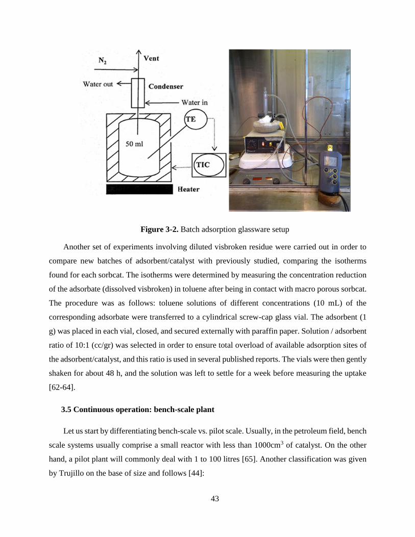
3.4 BATCH ADSORPTION EXPERIMENTS ...................................................................................................... 42
3.5 CONTINUOUS OPERATION: BENCH-SCALE PLANT .................................................................................. 43
3.5.1 Process overview .............................................................................................................................. 44
3.5.2 Brief operation procedures ............................................................................................................... 48
3.6 FEED AND PRODUCT CHARACTERIZATION TECHNIQUES ........................................................................ 49
3.6.1 P-value (pv) ...................................................................................................................................... 49
3.6.2 Elemental analysis ............................................................................................................................ 49
3.6.3 High temperature simulated distillation (HTSD) ASTM D-7169-2005 ............................................ 50
Page 7
vi
3.6.4 Microcarbon Residue method ........................................................................................................... 50
3.6.5 Microdesasphalting .......................................................................................................................... 51
3.6.6 Thermal Gravimetric Analysis (TGA) ............................................................................................... 52
3.6.7 Gases ................................................................................................................................................ 52
3.6.8 Surface area ...................................................................................................................................... 52
3.6.9 Viscosity ............................................................................................................................................ 53
3.7 EXPERIMENTAL PLAN ........................................................................................................................... 53
3.7.1 Adsorption ........................................................................................................................................ 53
3.7.2 Catalytic Steam Gasification ............................................................................................................ 54
3.7.3 Catalytic Steam Cracking (CSC) ...................................................................................................... 55
CHAPTER 4. RESULTS AND DISCUSSION .......................................................................................... 56
4.1 ADSORPTION ........................................................................................................................................ 56
4.1.1 Feed Preparation ....................................................................................................................... 56
4.1.2 Adsorbent/catalyst preparation and characterization ................................................................ 58
4.1.3 Batch adsorption experiments .................................................................................................... 61
4.1.4 Dynamic adsorption ................................................................................................................... 62
4.2 CATALYTIC STEAM GASIFICATION ....................................................................................................... 65
4.2.1 Athabasca vacuum residue catalytic steam gasification ............................................................ 65
4.2.2 Screening of the sorbcats ........................................................................................................... 67
4.2.3 Athabasca visbroken residue CSG tests ............................................................................................ 80
4.3 CATALYTIC STEAM CRACKING (CSC) .................................................................................................. 84
4.3.1 CSC repeatability with VB residue ................................................................................................... 84
4.3.2 Temperature effects on the catalytic steam cracking ........................................................................ 87
4.3.3 CSC kinetics ...................................................................................................................................... 93
4.3.4 Catalytic steam gasification after CSC ............................................................................................. 99
4.4 CLOSING REMARKS ............................................................................................................................. 100
CHAPTER 5. CONCLUSIONS/FUTURE WORK ................................................................................ 103
REFERENCES ................................................................................................................................................. 107
APPENDIX A .................................................................................................................................................. 113
AGU SOP. Reactivity/Gasification Unit .................................................................................................. 113
APPENDIX B .................................................................................................................................................. 126
APPENDIX C .................................................................................................................................................. 132
APPENDIX D .................................................................................................................................................. 137
Page 8
vii
List of Tables
Table 2-1 Typical refinery products after distillation fractioning [11] .................................... 7
Table 2-2 Common adsorption applications [26] .................................................................. 11
Table 2-3 Surface area and pore volume of catalysts used by Sosa [10] ............................... 13
Table 2-4. Properties of tested alumina particles [29] ........................................................... 14
Table 2-5. Particle size and specific surface of selected transition metal oxide nanoparticles
[30] ................................................................................................................................................ 15
Table 2-6. Kinetic constants for adsorption of Athabasca bitumen asphaltenes over kaolin and
kaolin sorbcats (using eq. 2-5) [10] .............................................................................................. 16
Table 2-7. Determined asphaltenes adsorption values over an iron surface [31] .................. 17
Table 2-8. Langmuir constants for Athabasca n-C7 asphaltenes adsorption over metal oxides
[18] ................................................................................................................................................ 18
Table 2-9. Hydrocarbon steam gasification reactions [10] .................................................... 19
Table 2-10. Adsorption reaction rate coefficients for catalytic reaction at different
temperatures (using eq. 2-5) [10] .................................................................................................. 23
Table 2-11. Activation energy for different catalysts [10] .................................................... 24
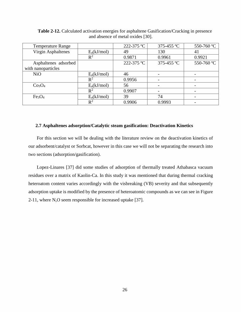
Table 2-12. Calculated activation energies for asphaltene Gasification/Cracking in presence
and absence of metal oxides [30]. ................................................................................................. 26
Table 4-1. Surface area and pore volume of the sorbcats tested ............................................ 58
Table 4-2. Surface area & pore volume of large and small scale preparation of 3NiO6K6Ba
sorbcat ........................................................................................................................................... 58
Page 9
viii
Table 4-3. Properties of the first two post-dynamic adsorption VB fractions ....................... 63
Table 4-4. Reactions occurring during catalytic steam gasification ...................................... 68
Table 4-5. Asphaltenes-LCO / 6K6Ca gas compositions for CSG experiment ..................... 69
Table 4-6. Global mass balance for 6K6Ba CSG of Asphaltenes-LCO ................................ 70
Table 4-7. Global mass balance comparison for the four studied sorbcats ........................... 75
Table 4-8. Gas rate, H2/CO2 & activation energy comparison for studied sorbcats in
asphaltenes-LCO CSG .................................................................................................................. 78
Table 4-9. Mass balance for 3NiO6K6Ba/VB experiment .................................................... 81
Table 4-10. Mass balance for 3NiO6K6Ba/VB during the CSG regeneration experiment ... 83
Table 4-11. CSG activation energies for 3NiO6K6Ba/VB both fresh and regenerated sorbcat
....................................................................................................................................................... 84
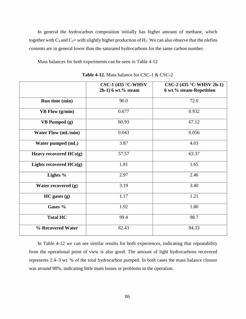
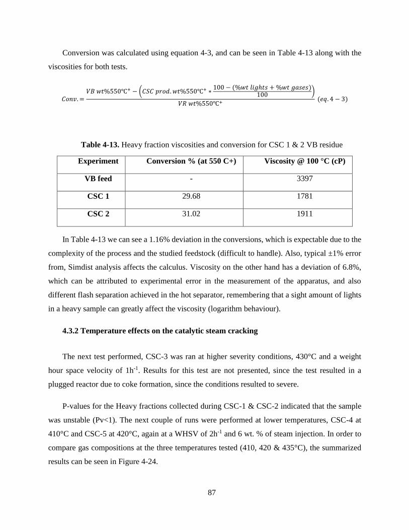
Table 4-12. Mass balance for CSC-1 & CSC-2 ..................................................................... 86
Table 4-13. Heavy fraction viscosities and conversion for CSC 1 & 2 VB residue .............. 87
Table 4-14. Mass balances for CSC 2, 4 & 5 (VB residue) ................................................... 90
Table 4-15. Conversion and viscosities for CSC 1, 2, 4 & 5 ................................................. 90
Table 4-16. Differential equations solved for the kinetic study of CSC ................................ 94
Table 4-17. Frequency factor and activation energy found for CSC reactions ..................... 99
Table C.1. Composition vs. Temperature for 6K6Ba ................................................... 132
Table C.2. Composition vs. Temperature for 3NiO6K6Ba .......................................... 133
Table C.3. Composition vs. Temperature for 3NiO6Cs6Ba ......................................... 134
Table C.4. Composition vs. Temperature for 3NiO6Cs6Ba with VB .......................... 135
Page 10
ix
Table C.5. Composition vs. Temperature for 3NiO6Cs6Ba with VB -Regenerated .... 136
Table D 1. Investment cost estimation for the visbreaking and CSC unit. ................... 137
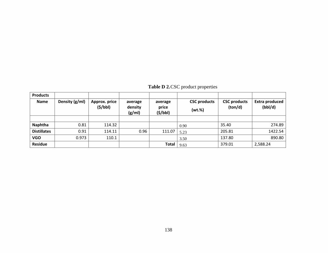
Table D 2. CSC product properties ............................................................................... 138
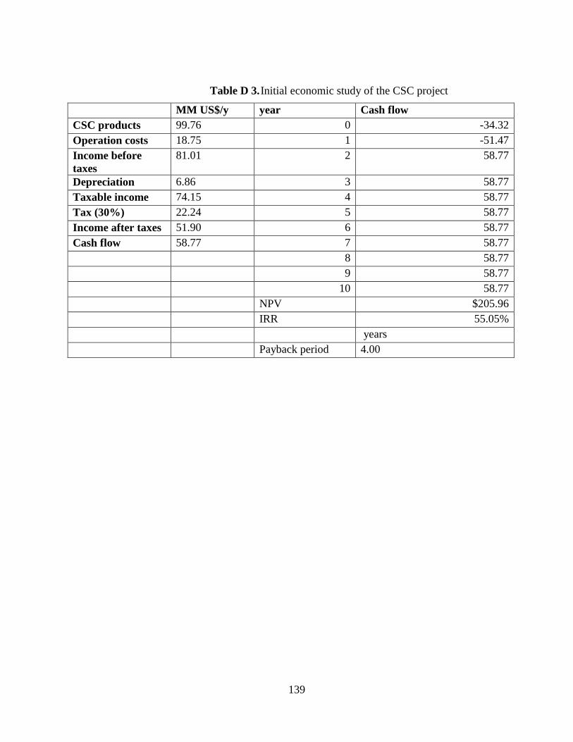
Table D 3. Initial economic study of the CSC project .................................................. 139
Page 11
x
List of Figures
Figure 1-1. Proposed process scheme [10] .............................................................................. 2
Figure 2-1 Schematic for a typical “high tech” refinery [11] .................................................. 6
Figure 2-2 Asphaltene molecule proposed by Carbognani. L.A. Blue atoms are nitrogen,
yellow atoms sulfur, red atoms oxygen, white atoms hydrogen and grey atoms carbon [22]. ....... 8
Figure 2-3. Typical tube visbreaker soaker configuration [15] ............................................. 10
Figure 2-4. Pore distributions of selected adsorbents measured by Mercury Intrusion
Porosimetry [28] ........................................................................................................................... 12
Figure 2-5. X ray diffractograms of calcined adsorbents [10] ............................................... 13
Figure 2-6. Kinetics of asphaltene adsorption derived from NIR data. Bulk concentration (C0):
1250 mg L-1 [31] .......................................................................................................................... 17
Figure 2-7. Variation of thermodynamic equilibrium for the system C-H2O with: A)
Temperature @ 1 bar; B) Pressure at 1000 K [10]. ...................................................................... 20
Figure 2-8. Electron microscopy of K-Ca(NO3)3/ graphite on a gold grid before reaction [33]
....................................................................................................................................................... 21
Figure 2-9. Energy-Dispersive-X-Ray spectroscopy (EDS) of parts A & B presented in Figure
2-8 [33].......................................................................................................................................... 22
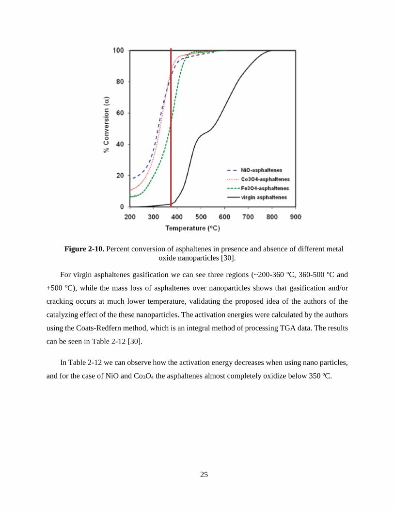
Figure 2-10. Percent conversion of asphaltenes in presence and absence of different metal
oxide nanoparticles [30]. ............................................................................................................... 25
Figure 2-11. Effect of heteroatoms on adsorption uptake over Kaolin-Ca [37] .................... 27
Figure 2-12. Reaction rates for graphite gasification over Ni/NiKOx catalyst [20] .............. 28
Figure 2-13. Effect of ash on NiK catalyst [38] ................................................................... 29
Page 12
xi
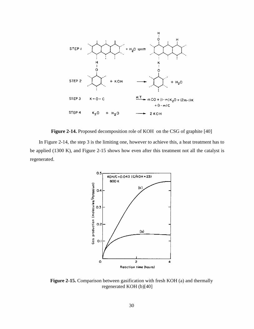
Figure 2-14. Proposed decomposition role of KOH on the CSG of graphite [40] ............... 30
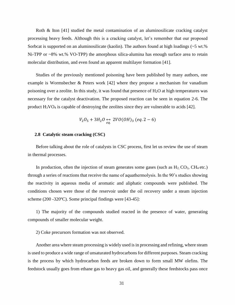
Figure 2-15. Comparison between gasification with fresh KOH (a) and thermally regenerated
KOH (b)[40].................................................................................................................................. 30
Figure 2-16. Setup used by Saraji and Goual for asphaltenes adsorption [54] ...................... 35
Figure 2-17. Experimental apparatus used by Delannay and Tysoe [40] .............................. 36
Figure 2-18. Experimental setup used by Pereira and Somorjai [36] .................................... 37
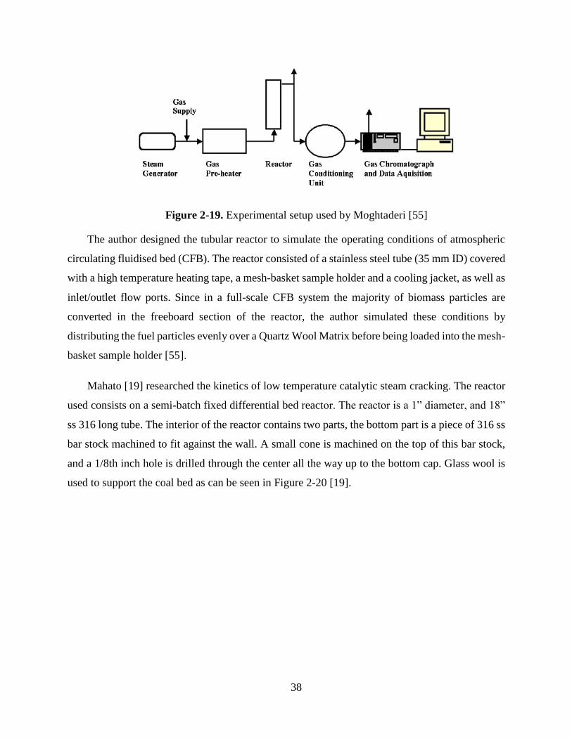
Figure 2-19. Experimental setup used by Moghtaderi [55] ................................................... 38
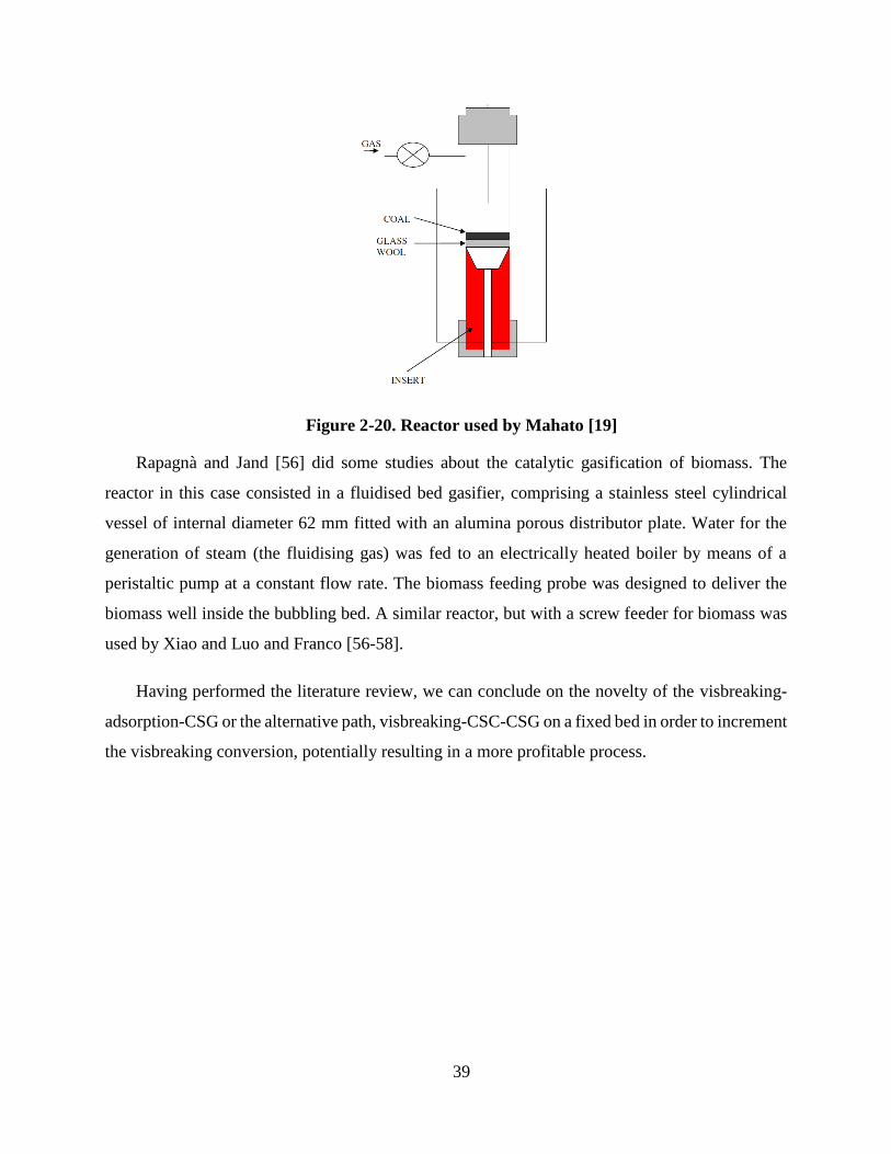
Figure 2-20. Reactor used by Mahato [19] ............................................................................ 39
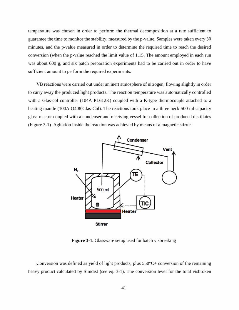
Figure 3-1. Glassware setup used for batch visbreaking ....................................................... 41
Figure 3-2. Batch adsorption glassware setup ....................................................................... 43
Figure 3-3. Schematic representation of the reactivity/gasification plant ............................. 46
Figure 3-4. Reactor for the asphaltenes reactivity/ catalytic steam gasification ................... 47
Figure 3-5. Schematic of the multi samples MCR setup [70] ............................................... 51
Figure 4-1 P-value versus time, visbroken feed preparation ................................................. 56
Figure 4-2. Simdist of Athabasca vacuum residue and VB Athabasca vacuum residue ....... 57
Figure 4-3. P-value determination for the visbroken vacuum residue ................................... 57
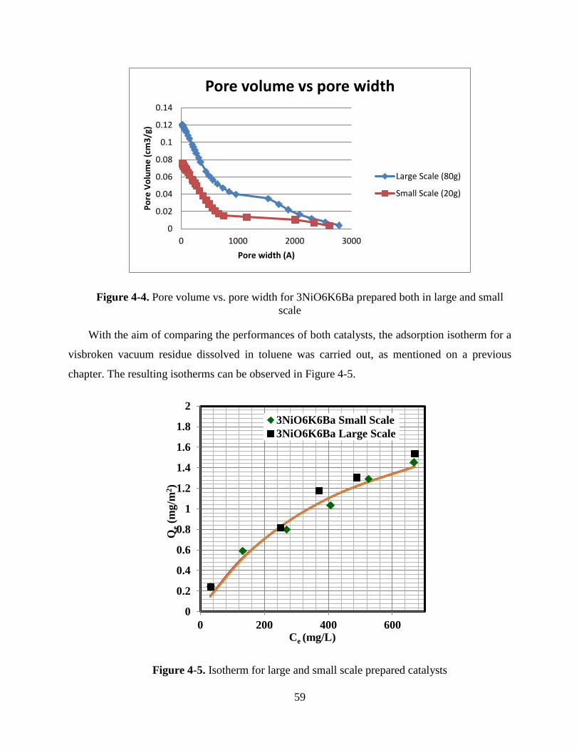
Figure 4-4. Pore volume vs. pore width for 3NiO6K6Ba prepared both in large and small scale
....................................................................................................................................................... 59
Figure 4-5. Isotherm for large and small scale prepared catalysts ......................................... 59
Figure 4-6. Evidence of nickel incorporation by SEM .......................................................... 60
Figure 4-7. Nickel distribution by XPS ................................................................................. 61
Page 13
xii
Figure 4-8. P-values for the VB prepared by Gonzalez [28] and the one used in this
investigation. ................................................................................................................................. 62
Figure 4-9. P-values for dynamic adsorption with 3NiO6K6Ba/Athabasca VB ................... 63
Figure 4-10. Alternative scheme for VB upgrading subsequent catalytic steam gasification 64
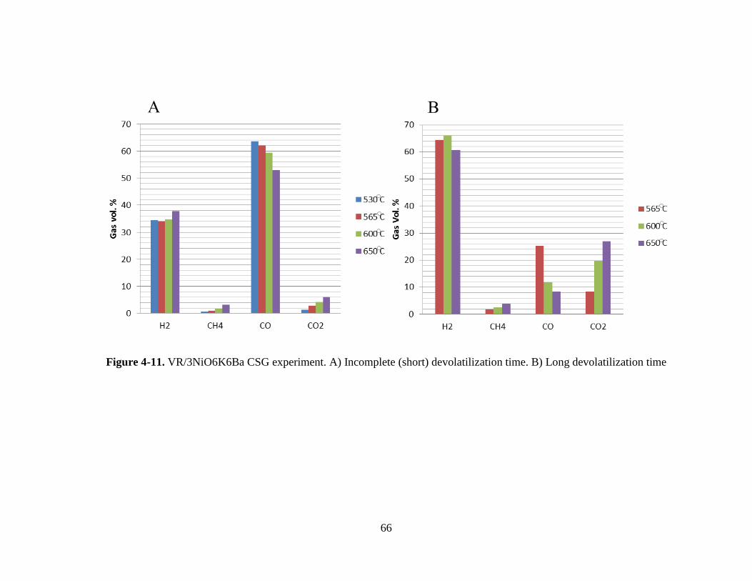
Figure 4-11. VR/3NiO6K6Ba CSG experiment. A) Incomplete (short) devolatilization time.
B) Long devolatilization time ....................................................................................................... 66
Figure 4-12. Gas composition for asphaltenes-LCO / 6K6Ca gas compositions for CSG
experiments ................................................................................................................................... 67
Figure 4-13. Gas chromatography example for a CSG sample ............................................. 68
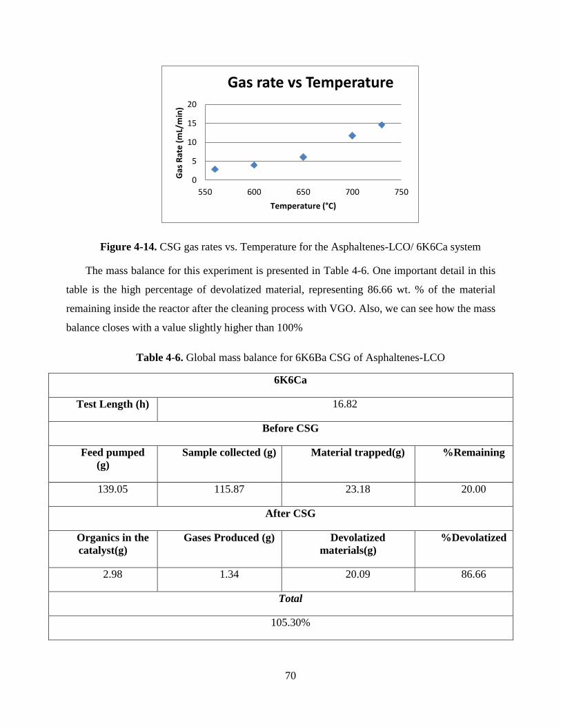
Figure 4-14. CSG gas rates vs. Temperature for the Asphaltenes-LCO/ 6K6Ca system ...... 70
Figure 4-15. TGA result for spent 6K6Ca top section spent catalyst. ................................... 71
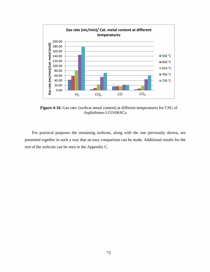
Figure 4-16. Gas rate/ (sorbcat metal content) at different temperatures for CSG of
Asphaltenes-LCO/6K6Ca ............................................................................................................. 72
Figure 4-17.Gas composition (Vol. %) at different temperatures comparison for the four
sorbcats ......................................................................................................................................... 73
Figure 4-18. Comparison of gas rate/cat metal content at different temperatures for the four
studied sorbcats in asphaltene-LCO CSG ..................................................................................... 77
Figure 4-19. Gas rate and H2/CO2 comparison for the four sorbcats @ 650 °C asphaltenes-
LCO CSG ...................................................................................................................................... 79
Figure 4-20. Activation energies for the four sorbcats @ 650 °C asphaltenes-LCO CSG .... 79
Figure 4-21. Composition (Vol. %) at different temperatures for 3NiO6K6Ba/ VB experiment
....................................................................................................................................................... 80
Page 14
xiii
Figure 4-22. Composition (Vol. %) at different temperatures for 3NiO6K6Ba/ VB
regeneration experiment................................................................................................................ 82
Figure 4-23. Gas composition for CSC-1 &CSC-2 carried out with VB residue .................. 85
Figure 4-24. Gas composition for CSC 2, 4 &5 .................................................................... 88
Figure 4-25. Gas composition comparison for CSC5 & 6 ..................................................... 91
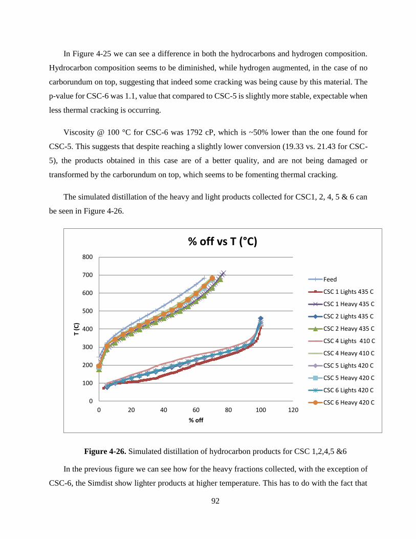
Figure 4-26. Simulated distillation of hydrocarbon products for CSC 1,2,4,5 &6 ................ 92
Figure 4-27. Proposed lump-compositions kinetic model ..................................................... 94
Figure 4-28. Kinetic constant calculation scheme ................................................................. 96
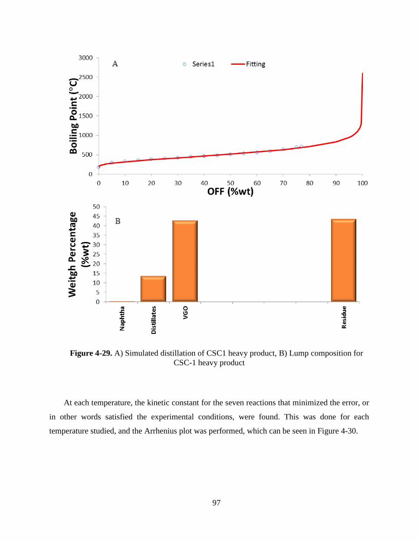
Figure 4-29. A) Simullated distillation of CSC1 heavy product, B) Lump composition for
CSC-1 heavy product .................................................................................................................... 97
Figure 4-30. Arrhenius plot for the proposed lump model reaction system .......................... 98
Figure 4-31. Comparison between CSG after asphaltenes-LCO adsorption and after CSC 100
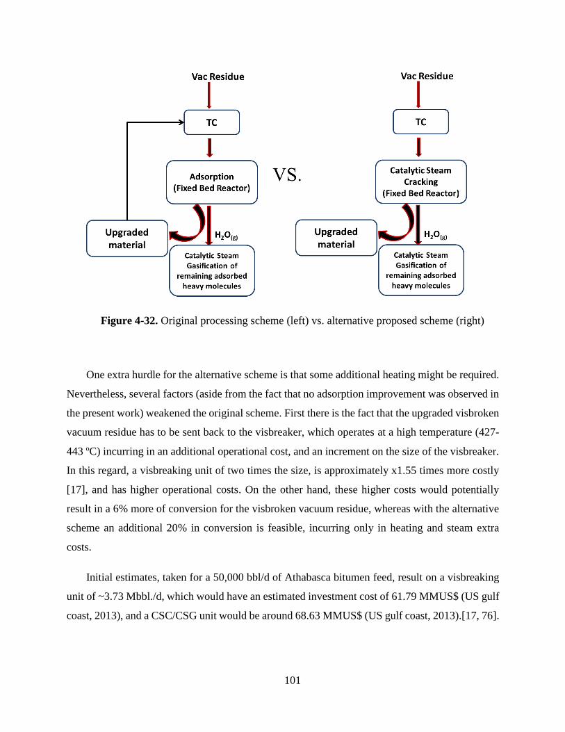
Figure 4-32. Original processing scheme (left) vs. alternative proposed scheme (right) .... 101
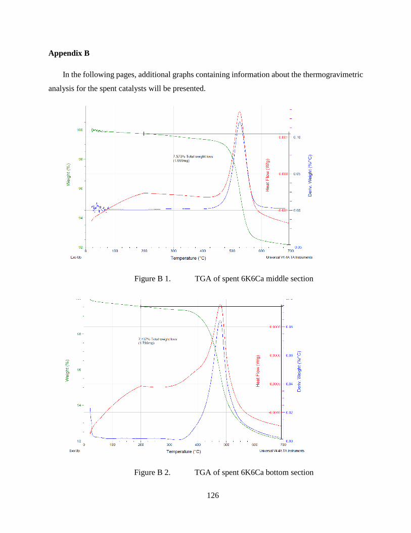
Figure B 1. TGA of spent 6K6Ca middle section .......................................................... 126
Figure B 2. TGA of spent 6K6Ca bottom section.......................................................... 126
Figure B 3. TGA of spent 6K6Ba top section ................................................................ 127
Figure B 4. TGA of spent 6K6Ba middle section .......................................................... 127
Figure B 5. TGA of spent 6K6Ba Bottom section ......................................................... 128
Figure B 6. TGA of spent 3NiO6K6Ba top section ....................................................... 128
Figure B 7. TGA of spent 3NiO6K6Ba middle section ................................................. 129
Figure B 8. TGA of spent 3NiO6K6Ba bottom section ................................................. 129
Page 15
xiv
Figure B 9. TGA of spent 3NiO6Cs6Ba top section...................................................... 130
Figure B 10. TGA of spent 3NiO6Cs6Ba middle section................................................ 130
Figure B 11. TGA of spent 3NiO6Cs6Ba bottom section ............................................... 131
Figure C.1. Gas rate vs. temperature for 6K6Ba ............................................................ 132
Figure C.2. Gas rate vs. temperature for 3NiO6K6Ba ................................................... 133
Figure C.3. Gas rate vs. temperature for 3NiO6Cs6Ba ................................................. 134
Figure C.4. Gas rate vs. temperature for 3NiO6Cs6Ba with VB ................................... 135
Figure C.5. Gas rate vs. temperature for 3NiO6Cs6Ba with VB -Regenerated ............ 136
Page 16
xv
List of Symbols, Abbreviations, Nomenclatures
Symbol Description
AGU Adsorption gasification unit
BET Brunauer–Emmett–Teller
cc Cubic centimeters
CFB Circulating fluidised bed
Cm Centimeter
CMC Carbon Management Canada
CSC Catalytic Steam cracking
CSG Catalytic steam gasification
CUT Catalytic upgrading technology
EDS Energy dispersive X-ray spectroscopy
FCC Fluid catalytic cracking
Fwusa Foster wheeler USA
g Grams
GC Gas chromatography
HTSD High temperature simulated distillation
LCO Light cycle oil
LGO Light gas oil
LPG Liquefied petroleum gas
mg Milligrams
mL Millilitres
MCR Micro carbon residue
min Minute
Pv P-value
RA Relative absorbance
R&D Research and development
SAGD Steam assisted gravity drainage
SCSC Selective catalytic steam cracking
Simdist Simulated distillation
SOP Standard operative procedure
TBP True boiling point
TGA Thermo gravimetric analysis
VB Visbroken
VGO Vacuum gasoil
VR Vacuum residue
WHSV Weight hourly space velocity
XRD X-ray diffraction
Page 17
1
Chapter 1. Introduction
1.1 Background
Unconventional oil is set to play an increasingly important role in world oil supply through to
2035, where Canadian oil sands and Venezuelan extra-heavy oil are expected to dominate the
market. Global primary energy demand will continue to grow, but at a slower rate than in recent
decades, and by 2035, it is predicted to be 36% higher than in 2008 [1].
In this sense, Alberta’s oil sands resource, which is comparable to Saudi Arabia in the size of
reserves, has been gaining weight as a strategic North American energy supply. After around 40
years of commercial production, a new development strategy is making a production of 5 million
a day a possibility, which would mean approximately 16% of North American demand by 2030,
creating potentially thousands of jobs throughout Canada, and a good target to develop new
technologies and process alternatives due to the nature of the oil sands [2].
At present, oil sands production faces several challenges that need to be addressed in order to
make it sustainable in the long run. Some of these challenges are: I) Crude oil prices, since oil
sands are expensive to produce and a significant drop in the price could lead to bad economics for
many existing and potential projects; II) Capital costs: Oil sands projects, in particular those
involving upgrading, are capital intensive; III) Natural gas costs, since both mining and thermal in
situ operations require a high amount of natural gas, among other things to produce the vital
hydrogen used in upgrading [3]. The future price of natural gas and the development of
alternatives, including gasification, will have a direct impact on project economics; IV) Diluent
availability, with the production of diluents declining and their demand increasing, the prices for
diluent are rising; V) Technology; since technology has enabled gradual reductions in supply costs,
and improvements in general upgrading costs are expected as new and improved upgrading
technologies are employed [4].
Following the preceding, hydrogen demand is constantly increasing since the use of heavy
hydrocarbons is growing. Of the total hydrogen production, 40% is used in chemical processes,
40% in refineries and 20% for other uses. In 2003, 48% of the global hydrogen demand was
Page 18
2
produced from natural gas, 30% from oil and recovered from refinery/chemical industry off-gases,
18% from coal, and 4% from electrolysis. Most of this hydrogen is produced on-site in refinery
and chemical plants for captive, non-energy uses [5]. Combining this to the fact that natural gas
consumption is increasing rapidly, new ways of cheap and clean hydrogen production have to be
found [6].
Heavier crudes also translate in feeds richer in asphaltenes, which are hetero-polyaromatic
compounds of large molecular weight, ranging from 700 to 2000 g/mol [7]. In the industry, these
compounds tend to precipitate and cause all sorts of operational problems, ranging from catalysts
poisoning to pipe plugging [8],[9].
Keeping the hydrogen demand increase and asphaltenes challenges in mind, an innovative
process was proposed by the Catalysis for Bitumen Upgrading and Hydrogen Production research
group at the University of Calgary, under funding support of Carbon Management Canada (CMC).
This new process attempts to provide at least a partial solution to both problems. It consists of
selectively segregating the unstable fractions of asphaltenes by adsorbing a few layers of them on
an in-house designed adsorbent/catalytic (sorbcat) matrix to further produce hydrogen via catalytic
steam gasification (CSG) of adsorbed asphaltenes at lower temperature than conventional thermal
gasification as can be seen in the scheme (see Figure 1-1) [10].
Figure 1-1. Proposed process scheme [10]
Page 19
3
1.2 Thesis objectives
The primary objective of the present study is to determine the feasibility of the proposed
process, which main goal is to improve the nature visbroken vacuum residue for further uses, thus
obtaining more valuable products, and also the production of hydrogen by CSG of the most
undesirable unstable hydrocarbon molecules. The specific objectives of this work are:
1 Designing and building a bench-scale set up capable of performing both continuous
adsorption and catalytic steam gasification of heavy hydrocarbon feeds
2 Screening of the different in-house adsorbent/catalysts produced by the group using a feed
consisting of C7 asphaltenes isolated from an industrial source
3 Visbroken vacuum residue feed production
4 Perform the adsorption and subsequent CSG tests with the visbroken vacuum residue feed
5 Catalytic steam cracking tests using the visbroken vacuum residue feed
Page 20
4
Chapter 2. Literature review
Understanding the different types of feedstock processed on a refinery is important to grasp
and idea of the challenges several streams present. Along the same line, some technologies
available, such as visbreaking, gasification etc. are studied in order to understand what’s currently
being implemented for heavy oil upgrading, providing us with an insight of the benefits and
weaknesses of the processes being implemented, in order to come up with a novel refining
proposal.
2.1 Feedstocks
Petroleum, which once produced is called crude oil, is perhaps the most important commodity
consumed in the world nowadays. From a chemical point of view, comprises a complex mixture
of hydrocarbon compounds, with some heteroatoms (minor amounts) such as nitrogen, oxygen
and sulfur, as well as some traces of metals-containing compounds. This mixture varies in the
amount of heteroatoms, volatility, specific gravity, and viscosity. The fuels derived from this
mixture, such as gasoline, kerosene and diesel provide the fuel for automobiles, tractors, aircrafts
and ships. The remainder includes fuel oil and natural gas used to heat homes and commercial
buildings, and materials used by the petrochemical industry to manufacture from synthetic clothing
fibers, to plastics fertilizers and paints [11, 12].
Heavy crude oils are less conventional and much more difficult to recover from the subsurface
reservoir. These materials have higher viscosity and Lower API gravity than conventional
petroleum, usually requiring thermal stimulation of the reservoir [11].
Let’s recall that viscosity is equal to the shear stress/shear rate, or in a less abstract way, it’s
commonly defined as the resistance to flow, and the API gravity, which stands for American
Petroleum Institute gravity, is calculated from the specific gravity of an oil, which is the ratio of
its density to that of water at 60 ºF (15.6 ºC), following the formula presented below. API gravity
is derived from the old Reaumur scale and does not have units, but is commonly referred as
degrees, and moves inversely to density, meaning the denser the oil is, the lower the API gravity
is presented in equation 2-1 [13, 14].
Page 21
5
𝐴𝑃𝐼 𝑔𝑟𝑎𝑣𝑖𝑡𝑦 = (141.5
𝑆𝑝𝑒𝑐𝑖𝑓𝑖𝑐 𝐺𝑟𝑎𝑣𝑖𝑡𝑦) − 131.5 (𝑒𝑞. 2 − 1)
Petroleum and heavy oil were generally defined in terms of physical properties, for example,
heavy oils were considered to be those crude oils having API gravity somewhat less than 20° API
(commonly falling into the range 10° to 15°), and extra heavy oils, such as tar sand bitumen,
usually have an API gravity in the range 5° to 10° (like Athabasca bitumen with 8° API). The term
heavy oil has also been used to describe both the heavy oils that require thermal stimulation to the
reservoir to be recovered and the bitumen contained in bituminous sand formations from which
the heavy bituminous material is recovered by mining operations [11].
The term bitumen includes a wide variety of semi-solid, very viscous and even sometimes
brittle materials that exist in nature. Natural bitumen is a material found in deposits with low
permeability in which the passage of fluids can only be achieved by fracturing techniques. On the
other hand, tar sand bitumen is a heavy hydrocarbon mixture with little material boiling below 350
°C. Tar sands have been defined in the United States as “the several rock types that contain an
extremely viscous hydrocarbon which is not recoverable in its natural state by conventional oil
well production methods including currently used enhanced recovery techniques”. The term oil
sand is also commonly used in the same way as the term tar sand, and these terms are frequently
used interchangeably. In conclusion, to differentiate bitumen, heavy oil, and conventional
petroleum, the use of a one physical parameter (such as viscosity) is not enough. Usually the
properties of the bulk deposit plus the required recovery methods form the basis for the definition
of these materials [11].
2.2 Refining Schemes
Oil refining consists not only on the separation of petroleum into fractions, but also comprises
all the subsequent treating of these fractions to yield marketable products. A refinery is essentially
a group of plants involving different processes which vary in number according with the products
produced (for example see Figure 2-1). The typical fuels refinery goal is the conversion of as much
of crude oil into transportation fuels as is economically viable. Although refineries produce many
lucrative products, high-volume profitable products are the transportation fuels such as gasoline,
diesel and turbine (jet) fuels, and the light heating oils. Also, a refinery must be flexible and be
Page 22
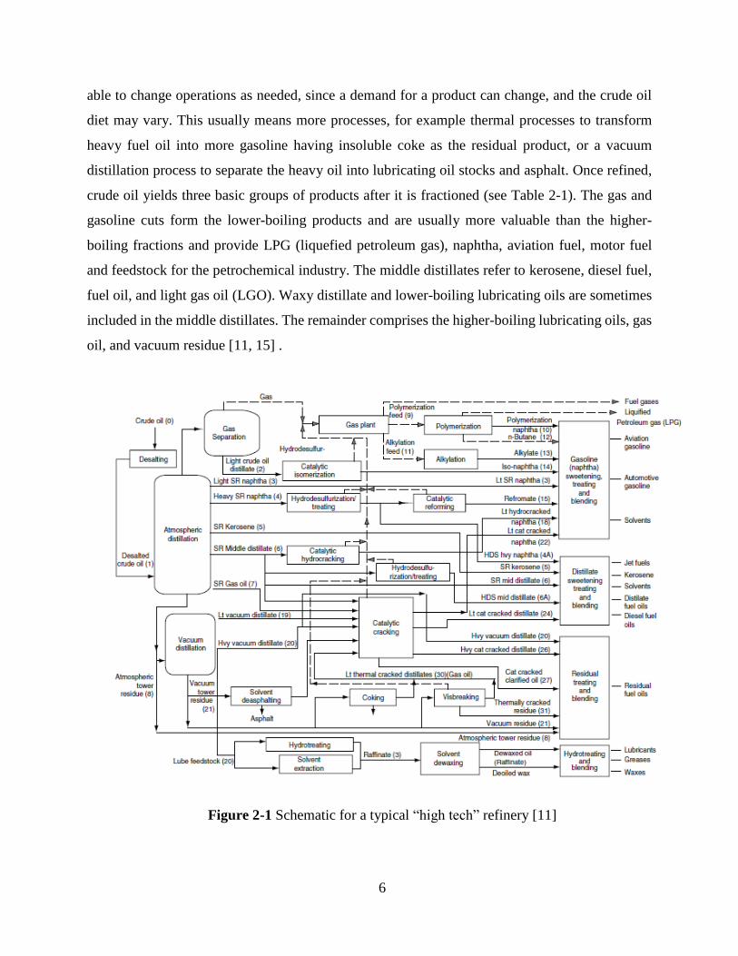
6
able to change operations as needed, since a demand for a product can change, and the crude oil
diet may vary. This usually means more processes, for example thermal processes to transform
heavy fuel oil into more gasoline having insoluble coke as the residual product, or a vacuum
distillation process to separate the heavy oil into lubricating oil stocks and asphalt. Once refined,
crude oil yields three basic groups of products after it is fractioned (see Table 2-1). The gas and
gasoline cuts form the lower-boiling products and are usually more valuable than the higher-
boiling fractions and provide LPG (liquefied petroleum gas), naphtha, aviation fuel, motor fuel
and feedstock for the petrochemical industry. The middle distillates refer to kerosene, diesel fuel,
fuel oil, and light gas oil (LGO). Waxy distillate and lower-boiling lubricating oils are sometimes
included in the middle distillates. The remainder comprises the higher-boiling lubricating oils, gas
oil, and vacuum residue [11, 15] .
Figure 2-1 Schematic for a typical “high tech” refinery [11]
Page 23
7
Table 2-1 Typical refinery products after distillation fractioning [11]
Boiling range
Fraction °C °F
Light naphtha -1-150 30-300
Gasoline -1-180 30-355
Heavy naphtha 150-205 300-400
Kerosene 205-260 400-500
Light gas oil 260-315 500-600
Heavy gas oil 315-425 600-800
Lubricating oil >400 >750
Vacuum gas oil 425-600 800-1100
Vacuum residue >510 >950
The recent high prices of crude oil and the use of heavier feeds as we will see later, has affected
the refining industry demanding new and more efficient ways to process tar sands, while coal
gasification and synthesis of fuels have been gaining importance. Adding stricter environmental
regulations to the equation (which imply higher costs), results in a re-shaping of modern refineries
in order to produce less expensive fuels [16].
2.3 Heavy crude oil upgrading
As we mentioned before, refining refers to the industry for transforming crude oil from various
origins into a specific set of products, varying with the specifications and demands of the market
[17]. Petroleum refining is currently undergoing a transition period, although the demand for
hydrocarbon and its products has shown a sharp growth in recent years, it is said this might be the
last century for petroleum refining as we conventionally know it. Over the last decades the API
gravity of crude oils available for the refineries has decreased. However this trend has moved the
industry to look for new ways to convert those heavy crude oils into low-boiling high-value
Page 24
8
products, facing the challenges this heavy and extra heavy feed present, such as an increased
asphaltenes content, and increases in sulfur, metal, and nitrogen contents [11].
There is a limitation for the processing of the mentioned heavy feedstocks, and that depends
largely on the amount of high molecular weight constituents like asphaltenes, which contain the
majority of heteroatoms and metals, known to poison catalysts and shorten their active life. Let’s
remember that asphaltenes are hetero-polyaromatic compounds of large molecular weight, ranging
from 700 to 2000 g/mol (see Figure 2-2). It is important to mention that there are other
representations with less aromatic domains, such as the “archipelagos” types of molecules. These
constituents are responsible for high yields of coke. Petroleum coke is a solid product of the
destructive distillation of petroleum derivatives, whenever these materials are heated over their
decomposition temperature. Visual appearance of this material is similar to that of coal, and it is
insoluble in any known solvent. This material also causes several problems going from the
deactivation of catalysts, to mechanical problems such as pipe plugging and fouling [11, 18-21].
Figure 2-2 Asphaltene molecule proposed by Carbognani. L.A. Blue atoms are nitrogen,
yellow atoms sulfur, red atoms oxygen, white atoms hydrogen and grey atoms carbon [22].
Page 25
9
Current technologies for heavy crude oil upgrading and residue can be roughly divided into
the processes involving carbon rejection and those involving hydrogen addition. Carbon rejection
redistributes hydrogen among the different products, resulting in fractions with an increased H/C
atomic ratio, and some others with a lower H/C atomic ratio. Within the most common
technologies we have [11]:
Carbon rejection: Visbreaking, coking and fluid catalytic cracking (FCC)
Hydrogen addition: Hydrovisbreaking and catalytic hydrocracking
2.4 Visbreaking
There’s some confusion between the terms visbreaking and thermal cracking, since both
processes tend to decrease the viscosity of the feedstock. The difference is based not only on the
type of feedstock, but on the severity of cracking. Moreover, the term visbreaking should refer
strictly to the viscosity reduction of heavy stock as the process’s main objective [23].
The soak visbreaker process configuration is similar to a single stage thermal cracker but
usually an additional equipment is added after the heater, consisting on a soaking drum which
prolongs the time the heater effluent remains at the cracking temperature (without being subjected
to further heat input and temperature). The objective is to maintain good fuel oil stability while
still converting sufficient of the feed thus lowering the residue viscosity. After the soaker, there’s
a quenching stage using some recycled oil, and a fractionation of the product mixture. The severity
of the whole process is controlled by the flow rate through the furnace and the temperature; typical
conditions are around 427-443 ºC with a residence time of 2-6 min. Additionally, the operation
has to be stopped every 3-6 months (in the case of the coil visbreaker) to remove solids and coke
formation inside the tubes. This process configuration is shown as Figure 2-3 [11, 15, 23-25].
Page 26
10
Figure 2-3. Typical tube visbreaker soaker configuration [15]
Visbreaking typically produces 10% vol. of gasoline and lighter materials, depending of
course on the nature of the feedstock, however the yield is controlled by the stability of the
visbroken product; this parameter of stability is often measured by a technique called p-value. The
P-value technique consists on determining the required amount of hexadecane necessary to
precipitate the asphaltenes on a sample, and that will be discussed on a later chapter.
2.5 Adsorption
When a solid is in contact with a fluid, whether it is a gas or a liquid, the existent interaction
forces between the molecules in the fluid matrix (or adsorbate) and the surface of the solid can
form a bond, and this process receives the name of adsorption. This process follows several steps,
first we have the diffusion of the adsorbate from the fluid to the external surface of the adsorbent,
then the adsorbate is diffused through the pores until is adsorbed in the internal surface. The
strength of these interactions will depend on both the nature of the adsorbate and that of the solid,
and can also be affected by steric impediment [26, 27].
In the last 30 years, adsorption has become a key separation technique in the oil industry. The
usual applications for this process involve purification of specific streams as can be seen in Table
Page 27
11
2-2. Adsorption is also used in those cases where the distillation of a mixture is difficult, such as
isomer mixtures, and substances with similar boiling points [26].
Table 2-2 Common adsorption applications [26]
Feed Principal product Adsorbent Adsorbate
Air O2 Zeolite 4Å, 5Å N2
H2/CH4 H2 Zeolite 3Å, 4Å
Carbon sieve
CH4
n/isoparaffines
C4-C6
isoparaffines Zeolite 5 Å n-Paraffines
n/isoparaffines
C10-C14
n-paraffines Zeolite 5 Å n-Paraffines
n-C4=/i-C4= n-C4= Zeolite 5 Å n-C4=
Olefins/Paraffines Olefins Zeolite X Olefins
Aromatics in C8 p-xylene Zeolite X,Y p-xylene
In the following sections we will discuss on the previous studies found on asphaltenes
adsorption over different solids.
2.5.1 Asphaltene adsorption: adsorbents
Manuel Gonzalez [28] worked on asphaltenes adsorption over a natural silica alumina (Kaolin
powder). The author characterized the adsorbent (before impregnating with the gasification
catalyst) using N2 surface area with BET equation. Details of the preparation of this Sorbcat
(adsorbent/catalyst) will be discussed later [28].
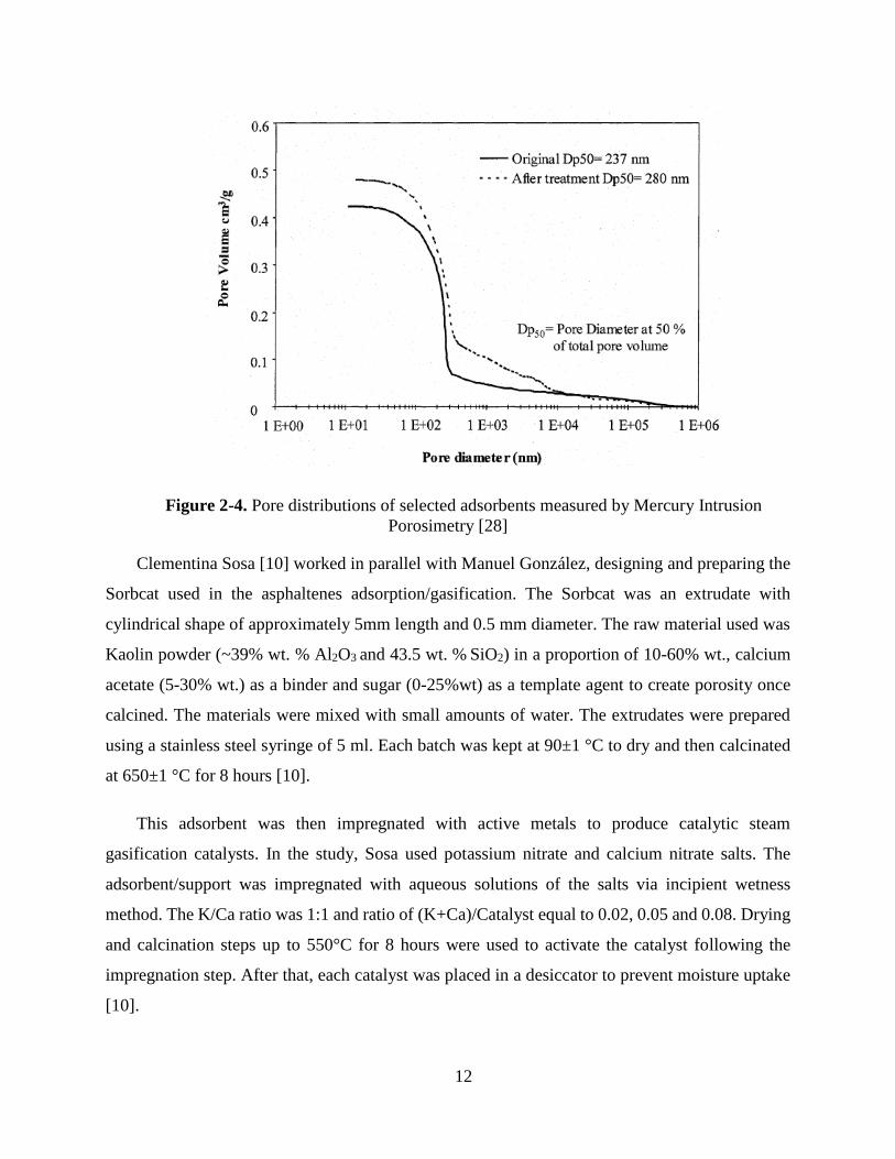
The surface area obtained was 10-12 m2/g. The pore volume of the Sorbcat measured by
Mercury Intrusion Porosimetry, had a maximum on 0.480 cm3/g, 14% higher compared to the
original kaolin (0.424 cm3/g), as can be seen in Figure 2-4 [28].
Page 28
12
Figure 2-4. Pore distributions of selected adsorbents measured by Mercury Intrusion
Porosimetry [28]
Clementina Sosa [10] worked in parallel with Manuel González, designing and preparing the
Sorbcat used in the asphaltenes adsorption/gasification. The Sorbcat was an extrudate with
cylindrical shape of approximately 5mm length and 0.5 mm diameter. The raw material used was
Kaolin powder (~39% wt. % Al2O3 and 43.5 wt. % SiO2) in a proportion of 10-60% wt., calcium
acetate (5-30% wt.) as a binder and sugar (0-25%wt) as a template agent to create porosity once
calcined. The materials were mixed with small amounts of water. The extrudates were prepared
using a stainless steel syringe of 5 ml. Each batch was kept at 90±1 °C to dry and then calcinated
at 650±1 °C for 8 hours [10].
This adsorbent was then impregnated with active metals to produce catalytic steam
gasification catalysts. In the study, Sosa used potassium nitrate and calcium nitrate salts. The
adsorbent/support was impregnated with aqueous solutions of the salts via incipient wetness
method. The K/Ca ratio was 1:1 and ratio of (K+Ca)/Catalyst equal to 0.02, 0.05 and 0.08. Drying
and calcination steps up to 550°C for 8 hours were used to activate the catalyst following the
impregnation step. After that, each catalyst was placed in a desiccator to prevent moisture uptake
[10].
Page 29
13
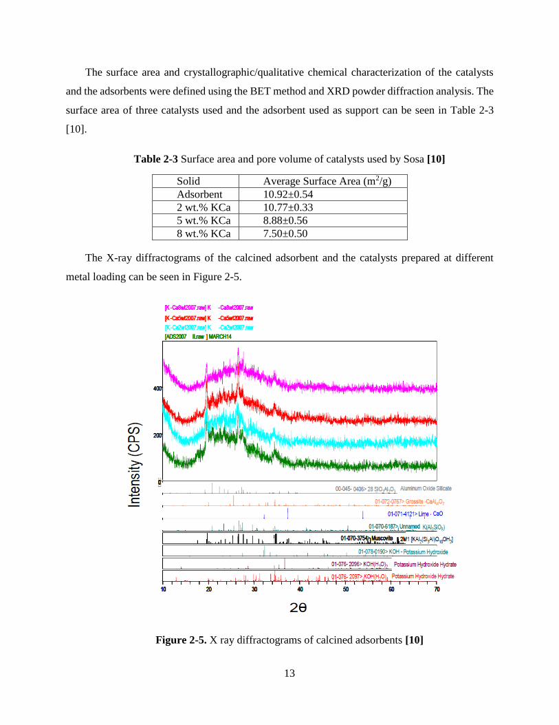
The surface area and crystallographic/qualitative chemical characterization of the catalysts
and the adsorbents were defined using the BET method and XRD powder diffraction analysis. The
surface area of three catalysts used and the adsorbent used as support can be seen in Table 2-3
[10].
Table 2-3 Surface area and pore volume of catalysts used by Sosa [10]
Solid Average Surface Area (m2/g)
Adsorbent 10.92±0.54
2 wt.% KCa 10.77±0.33
5 wt.% KCa 8.88±0.56
8 wt.% KCa 7.50±0.50
The X-ray diffractograms of the calcined adsorbent and the catalysts prepared at different
metal loading can be seen in Figure 2-5.
Figure 2-5. X ray diffractograms of calcined adsorbents [10]
Page 30
14
As can be seen in Figure 2-5, all the samples display a similar diffraction pattern consisting in
a highly amorphous phase with a small crystalline phase. The main signals are located between
16°<2θ<38° (where θ is the reflection angle). Metal loaded catalysts for catalytic steam
gasification application (CSG) did not show any difference upon the metal loading compared to
the adsorbent.
Nashaat Nassar and Azfar Hassan [29] studied the effect of particle size on asphaltenes
adsorption and oxidation, using alumina particles. The properties of the tested materials can be
seen in Table 2-4. The authors found that the adsorption capacity of the nano-alumina was higher
than that of the micro-alumina, on the other hand, micro-alumina showed higher catalytic activity
toward asphaltene oxidation than nano-alumina. This enhanced catalytic effect demonstrated by
micro-alumina shows that textural properties play an important role in catalysis [29].
Table 2-4. Properties of tested alumina particles [29]
Type X-ray
measured Particle
size
Specific
surface area
(BET) (m2/g)
Pore
volume (cm3/g)
Average
Pore Size (Å)
Nano 48±3 nm 39 - -
micro <200µm 156 0.2909 54
Nashaat Nassar and Azfar Hassan [30] also studied the adsorption and subsequent oxidation
of asphaltenes onto transition metal nanoparticles. Three types of transition metal oxide
nanoparticles, namely NiO, Co3O4 and Fe3O4 were used in this study. BET and external surface
areas are presented in Table 2-5. Particle size was determined by using X-ray Diffraction. Surface
areas of the nanoparticles were measured by a surface area and porosity analyzer. Surface area was
measured by performing N2-adsorption–desorption at 77 K using BET equation [30].
Page 31
15
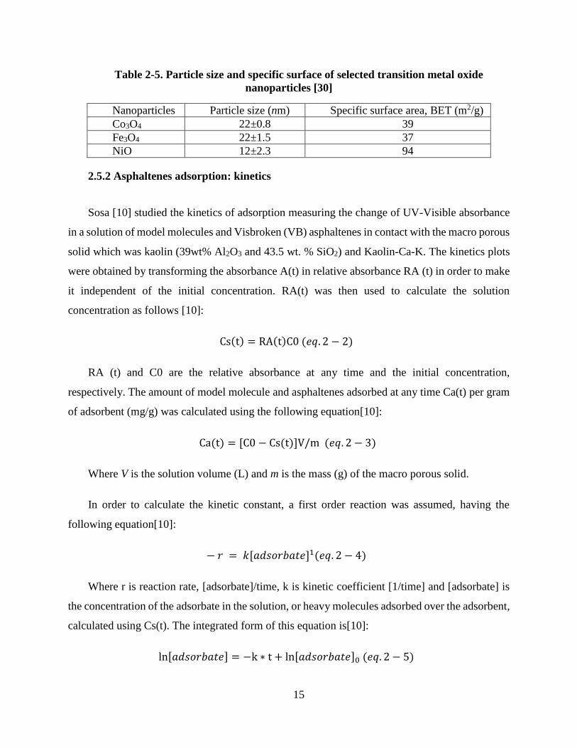
Table 2-5. Particle size and specific surface of selected transition metal oxide
nanoparticles [30]
Nanoparticles Particle size (nm) Specific surface area, BET (m2/g)
Co3O4 22±0.8 39
Fe3O4 22±1.5 37
NiO 12±2.3 94
2.5.2 Asphaltenes adsorption: kinetics
Sosa [10] studied the kinetics of adsorption measuring the change of UV-Visible absorbance
in a solution of model molecules and Visbroken (VB) asphaltenes in contact with the macro porous
solid which was kaolin (39wt% Al2O3 and 43.5 wt. % SiO2) and Kaolin-Ca-K. The kinetics plots
were obtained by transforming the absorbance A(t) in relative absorbance RA (t) in order to make
it independent of the initial concentration. RA(t) was then used to calculate the solution
concentration as follows [10]:
Cs(t) = RA(t)C0 (𝑒𝑞. 2 − 2)
RA (t) and C0 are the relative absorbance at any time and the initial concentration,
respectively. The amount of model molecule and asphaltenes adsorbed at any time Ca(t) per gram
of adsorbent (mg/g) was calculated using the following equation[10]:
Ca(t) = [C0 − Cs(t)]V/m (𝑒𝑞. 2 − 3)
Where V is the solution volume (L) and m is the mass (g) of the macro porous solid.
In order to calculate the kinetic constant, a first order reaction was assumed, having the
following equation[10]:
− 𝑟 = 𝑘[𝑎𝑑𝑠𝑜𝑟𝑏𝑎𝑡𝑒]1(𝑒𝑞. 2 − 4)
Where r is reaction rate, [adsorbate]/time, k is kinetic coefficient [1/time] and [adsorbate] is
the concentration of the adsorbate in the solution, or heavy molecules adsorbed over the adsorbent,
calculated using Cs(t). The integrated form of this equation is[10]:
ln[𝑎𝑑𝑠𝑜𝑟𝑏𝑎𝑡𝑒] = −k ∗ t + ln[𝑎𝑑𝑠𝑜𝑟𝑏𝑎𝑡𝑒]0 (𝑒𝑞. 2 − 5)
Page 32
16
Then plotting ln[adsorbate] versus time we should obtain a straight line whose slope is the
kinetic constant.
Results obtained for Athabasca bitumen C7- asphaltenes in toluene solution over macro porous
kaolin at 22 °C and its coefficients of determination can be seen in Table 2-6 [10].
Table 2-6. Kinetic constants for adsorption of Athabasca bitumen asphaltenes over kaolin
and kaolin sorbcats (using eq. 2-5) [10]
Compound K x10-3(min-1) R2
AB-Vacuum Residue (VR) 1.4±0.5 0.938
13.6 Visbroken VR 1.4±0.6 0.952
23.3 Visbroken VR 2.2±0.5 0.985
28.5 Visbroken VR 2.8±0.5 0.980
23.3 VB on K-Ca/Kaolin 2 wt.% 3.4±0.5 0.983
23.3 VB on K-Ca/Kaolin 8 wt.% 1.0±0.4 0.941
As we can observe, we are dealing with an apparent first order reaction, and that increasing
visbreaking severity seems to be increasing the kinetic constant obtained (severity is given by the
conversion in the first number of the compound name), being the proposed explanation that large
molecules present in the VR would be transformed into smaller ones depending on the severity of
the process, and this lower molecular size molecules are expected to display higher adsorption
uptakes.
Balabin [31] have also studied the behavior of petroleum asphaltenes on an iron surface using
near-infrared spectroscopy (NIR) and Raman microscopy. The author utilizes asphaltenes
extracted with petroleum ether in a 1:50 (v/v) ratio at 200 ºC from a mixture of West-Siberian
crude oils. The solvent utilized was benzene, and the adsorbent consisted on iron sheets (99.5%)
and iron foil. Experimental results show Langmuir type isotherms as can be seen in Figure 2-6,
Also, the parameters found by can be seen in Table 2-7 where Γmax is the maximum adsorbed
mass density; K=ka/kd is the adsorption equilibrium constant (ka and kd are the rate constants of
adsorption and desorption respectively) [31].
Page 33
17
Figure 2-6. Kinetics of asphaltene adsorption derived from NIR data. Bulk concentration
(C0): 1250 mg L-1 [31]
Table 2-7. Determined asphaltenes adsorption values over an iron surface [31]
measured calculated
Technique Γmax [mg m-2] K [L mg-1] Kads x106 [L
mg-1 min-1]
Kdes x106 [min-1] -ΔGads [kJ
mol-1]
Near infrared
(NIR)
spectroscopy
4.90 ±0.07 0.084±0.007 4.95±0.06 59.2±0.2 34.2±0.2
Raman
microscopy
5.3±0.5 0.04±0.02 - - 31.8±1.3
Nassar [18] has studied batch adsorption of n-C7 asphaltenes extracted from Athabasca
vacuum residue, with toluene as solvent over metal oxide nano particles (Fe3O4, Co3O4, TiO2,
MgO, CaO, and NiO). The amount of adsorbed asphaltenes was obtained by thermogravimetric
analysis (TGA). The isotherms obtained were fitted to Langmuir model obtaining the results
shown in Table 2-8 [18].
Page 34
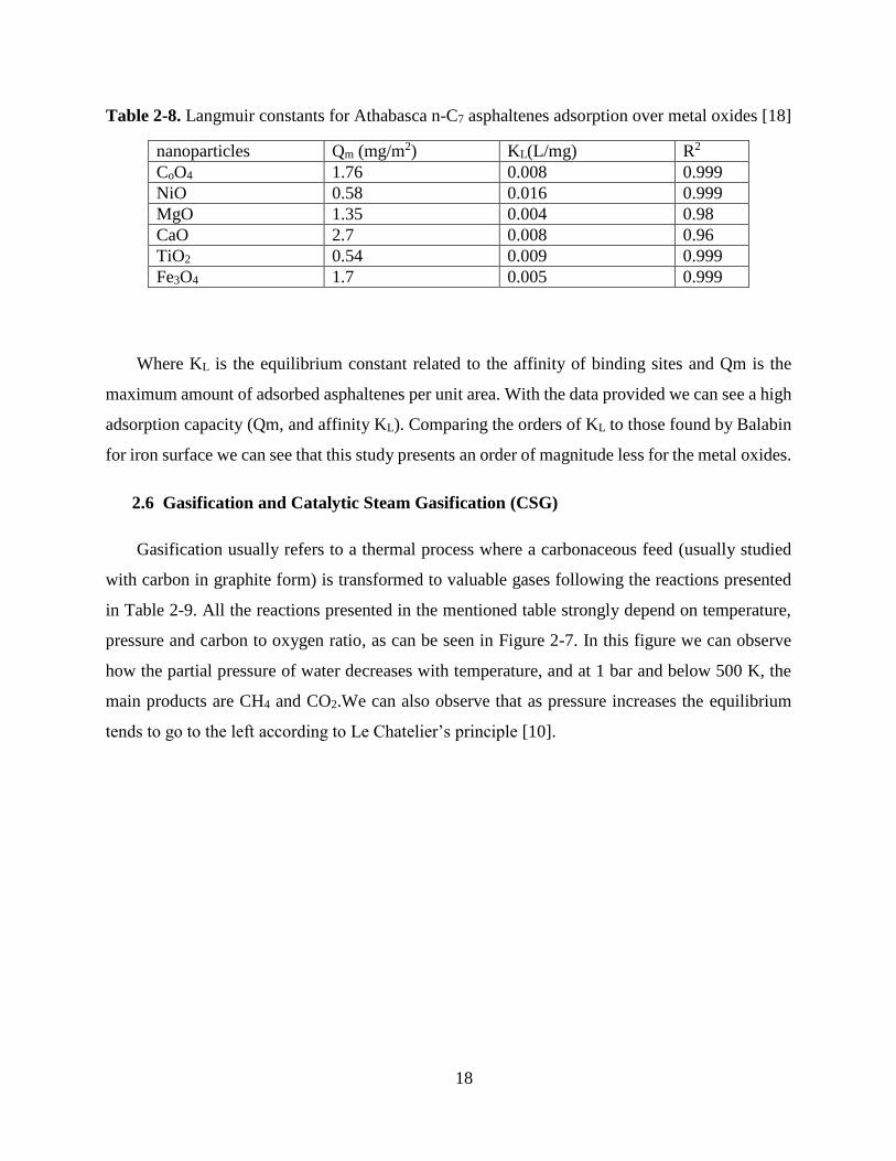
18
Table 2-8. Langmuir constants for Athabasca n-C7 asphaltenes adsorption over metal oxides [18]
nanoparticles Qm (mg/m2) KL(L/mg) R2
CoO4 1.76 0.008 0.999
NiO 0.58 0.016 0.999
MgO 1.35 0.004 0.98
CaO 2.7 0.008 0.96
TiO2 0.54 0.009 0.999
Fe3O4 1.7 0.005 0.999
Where KL is the equilibrium constant related to the affinity of binding sites and Qm is the
maximum amount of adsorbed asphaltenes per unit area. With the data provided we can see a high
adsorption capacity (Qm, and affinity KL). Comparing the orders of KL to those found by Balabin
for iron surface we can see that this study presents an order of magnitude less for the metal oxides.
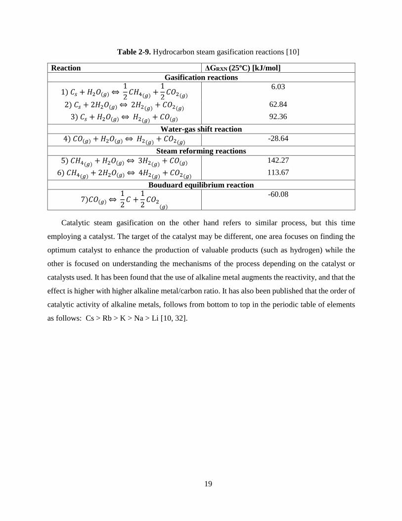
2.6 Gasification and Catalytic Steam Gasification (CSG)
Gasification usually refers to a thermal process where a carbonaceous feed (usually studied
with carbon in graphite form) is transformed to valuable gases following the reactions presented
in Table 2-9. All the reactions presented in the mentioned table strongly depend on temperature,
pressure and carbon to oxygen ratio, as can be seen in Figure 2-7. In this figure we can observe
how the partial pressure of water decreases with temperature, and at 1 bar and below 500 K, the
main products are CH4 and CO2.We can also observe that as pressure increases the equilibrium
tends to go to the left according to Le Chatelier’s principle [10].
Page 35
19
Table 2-9. Hydrocarbon steam gasification reactions [10]
Reaction ΔGRXN (25ºC) [kJ/mol]
Gasification reactions
1) 𝐶𝑠 + 𝐻2𝑂(𝑔)⇔ 1
2𝐶𝐻4(𝑔) +
1
2𝐶𝑂2(𝑔)
6.03
2) 𝐶𝑠 + 2𝐻2𝑂(𝑔)⇔ 2𝐻2(𝑔) + 𝐶𝑂2(𝑔) 62.84
3) 𝐶𝑠 + 𝐻2𝑂(𝑔)⇔ 𝐻2(𝑔) + 𝐶𝑂(𝑔) 92.36
Water-gas shift reaction
4) 𝐶𝑂(𝑔) + 𝐻2𝑂(𝑔)⇔ 𝐻2(𝑔) + 𝐶𝑂2(𝑔) -28.64
Steam reforming reactions
5) 𝐶𝐻4(𝑔) + 𝐻2𝑂(𝑔)⇔ 3𝐻2(𝑔) + 𝐶𝑂(𝑔) 142.27
6) 𝐶𝐻4(𝑔) + 2𝐻2𝑂(𝑔)⇔ 4𝐻2(𝑔) + 𝐶𝑂2(𝑔) 113.67
Bouduard equilibrium reaction
7)𝐶𝑂(𝑔)⇔ 1
2𝐶 +
1
2𝐶𝑂2
(𝑔)
-60.08
Catalytic steam gasification on the other hand refers to similar process, but this time
employing a catalyst. The target of the catalyst may be different, one area focuses on finding the
optimum catalyst to enhance the production of valuable products (such as hydrogen) while the
other is focused on understanding the mechanisms of the process depending on the catalyst or
catalysts used. It has been found that the use of alkaline metal augments the reactivity, and that the
effect is higher with higher alkaline metal/carbon ratio. It has also been published that the order of
catalytic activity of alkaline metals, follows from bottom to top in the periodic table of elements
as follows: Cs > Rb > K > Na > Li [10, 32].
Page 36
20
Figure 2-7. Variation of thermodynamic equilibrium for the system C-H2O with: A)
Temperature @ 1 bar; B) Pressure at 1000 K [10].
A
B
Page 37
21
2.6.1 Asphaltenes catalytic steam gasification: Catalysts
Pereira [33] studied the steam gasification of graphite and chars at temperatures below 1000K
over Potassium-Calcium-Oxide catalysts. The samples were impregnated with nitrate solutions of
potassium and calcium to incipient wetness, the atomic ratio was K/M+2=1 and K/C equal to 0.01.
The samples were then dried at 420 °C for one hour [33].
Electron Microscopy Study was used to characterize the catalyst distribution over the sample
before and after reaction. Figure 2-8 shows the distribution of K and Ca nitrates that can be
observed, as the dark spots which represent the areas with catalyst. Also the catalyst particles
varied in size having big particles denoted in the figure with the letter A, and smaller, letter B.
Energy-Dispersive-X-Ray spectroscopy (EDS) was used in the selected particles A & B in Figure
2-8, and the results are presented in Figure 2-9, where we can see that the spectra are almost
identical, indicating that the catalyst was thoroughly mixed [33].
Figure 2-8. Electron microscopy of K-Ca(NO3)3/ graphite on a gold grid before reaction
[33]
Page 38
22
Figure 2-9. Energy-Dispersive-X-Ray spectroscopy (EDS) of parts A & B presented in
Figure 2-8 [33].
Carrazza [34] worked with KOH and a transition metal oxide as a catalyst. This mix
(equimolar) was added to graphite by impregnation to incipient wetness. Separate solutions of
KOH and a water-soluble transition metal salt were used to deposit the desired loading of catalyst.
Nickel, iron, copper, cobalt and chromium nitrate, zinc and manganese sulfate, ammonium
metavanadate, and ammonium molybdate were used to deposit the respective metal oxide onto
graphite. A 0.5-g graphite sample was impregnated with 0.5 ml of the KOH and the metal salt
solutions. The sample was then dried in an oven at 393 K for 10 min, placed in the reactor and
Page 39
23
heated under He for half an hour at a temperature high enough to decompose the metal salt and
form the oxide. The gas flow over the sample was switched from He to steam and the rate of gas
formation and product distribution for the gasification of graphite with steam was followed at
different temperatures [34].
Similarly, Luis Pineda [35] studied the gasification of a SAGD depleted core impregnated
with catalyst. For the study the author used an equimolar solution of potassium nitrate and calcium
nitrate tetra hydrated as precursors of the catalyst. The precursor salts were introduced to the core
sample by impregnation to incipient wetness [35].
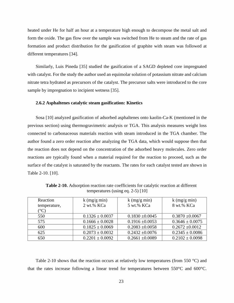
2.6.2 Asphaltenes catalytic steam gasification: Kinetics
Sosa [10] analyzed gasification of adsorbed asphaltenes onto kaolin-Ca-K (mentioned in the
previous section) using thermogravimetric analysis or TGA. This analysis measures weight loss
connected to carbonaceous materials reaction with steam introduced in the TGA chamber. The
author found a zero order reaction after analyzing the TGA data, which would suppose then that
the reaction does not depend on the concentration of the adsorbed heavy molecules. Zero order
reactions are typically found when a material required for the reaction to proceed, such as the
surface of the catalyst is saturated by the reactants. The rates for each catalyst tested are shown in
Table 2-10. [10].
Table 2-10. Adsorption reaction rate coefficients for catalytic reaction at different
temperatures (using eq. 2-5) [10]
Reaction
temperature,
(°C)
k (mg/g min)
2 wt.% KCa
k (mg/g min)
5 wt.% KCa
k (mg/g min)
8 wt.% KCa
550 0.1326 ± 0.0037 0.1830 ±0.0045 0.3870 ±0.0067
575 0.1666 ± 0.0028 0.1916 ±0.0053 0.3646 ± 0.0075
600 0.1825 ± 0.0069 0.2083 ±0.0058 0.2672 ±0.0012
625 0.2073 ± 0.0032 0.2432 ±0.0076 0.2345 ± 0.0086
650 0.2201 ± 0.0092 0.2661 ±0.0089 0.2102 ± 0.0098
Table 2-10 shows that the reaction occurs at relatively low temperatures (from 550 °C) and
that the rates increase following a linear trend for temperatures between 550°C and 600°C.
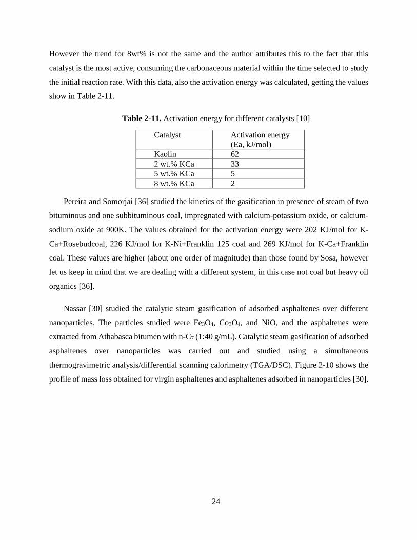
Page 40
24
However the trend for 8wt% is not the same and the author attributes this to the fact that this
catalyst is the most active, consuming the carbonaceous material within the time selected to study
the initial reaction rate. With this data, also the activation energy was calculated, getting the values
show in Table 2-11.
Table 2-11. Activation energy for different catalysts [10]
Catalyst Activation energy
(Ea, kJ/mol)
Kaolin 62
2 wt.% KCa 33
5 wt.% KCa 5
8 wt.% KCa 2
Pereira and Somorjai [36] studied the kinetics of the gasification in presence of steam of two
bituminous and one subbituminous coal, impregnated with calcium-potassium oxide, or calcium-
sodium oxide at 900K. The values obtained for the activation energy were 202 KJ/mol for K-
Ca+Rosebudcoal, 226 KJ/mol for K-Ni+Franklin 125 coal and 269 KJ/mol for K-Ca+Franklin
coal. These values are higher (about one order of magnitude) than those found by Sosa, however
let us keep in mind that we are dealing with a different system, in this case not coal but heavy oil
organics [36].
Nassar [30] studied the catalytic steam gasification of adsorbed asphaltenes over different
nanoparticles. The particles studied were Fe3O4, Co3O4, and NiO, and the asphaltenes were
extracted from Athabasca bitumen with n-C7 (1:40 g/mL). Catalytic steam gasification of adsorbed
asphaltenes over nanoparticles was carried out and studied using a simultaneous
thermogravimetric analysis/differential scanning calorimetry (TGA/DSC). Figure 2-10 shows the
profile of mass loss obtained for virgin asphaltenes and asphaltenes adsorbed in nanoparticles [30].
Page 41
25
Figure 2-10. Percent conversion of asphaltenes in presence and absence of different metal
oxide nanoparticles [30].
For virgin asphaltenes gasification we can see three regions (~200-360 ºC, 360-500 ºC and
+500 ºC), while the mass loss of asphaltenes over nanoparticles shows that gasification and/or
cracking occurs at much lower temperature, validating the proposed idea of the authors of the
catalyzing effect of the these nanoparticles. The activation energies were calculated by the authors
using the Coats-Redfern method, which is an integral method of processing TGA data. The results
can be seen in Table 2-12 [30].
In Table 2-12 we can observe how the activation energy decreases when using nano particles,
and for the case of NiO and Co3O4 the asphaltenes almost completely oxidize below 350 ºC.
Page 42
26
Table 2-12. Calculated activation energies for asphaltene Gasification/Cracking in presence
and absence of metal oxides [30].
Temperature Range 222-375 ºC 375-455 ºC 550-760 ºC
Virgin Asphaltenes Ea(kJ/mol) 49 130 41
R2 0.9871 0.9961 0.9921
Asphaltenes adsorbed
with nanoparticles
222-375 ºC 375-455 ºC 550-760 ºC
NiO Ea(kJ/mol) 46 - -
R2 0.9956 - -
Co3O4 Ea(kJ/mol) 56 - -
R2 0.9907 - -
Fe3O4 Ea(kJ/mol) 39 74 -
R2 0.9906 0.9993 -
2.7 Asphaltenes adsorption/Catalytic steam gasification: Deactivation Kinetics
For this section we will be dealing with the literature review on the deactivation kinetics of
our adsorbent/catalyst or Sorbcat, however in this case we will not be separating the research into
two sections (adsorption/gasification).
Lopez-Linares [37] did some studies of adsorption of thermally treated Athabasca vacuum
residues over a matrix of Kaolin-Ca. In this study it was mentioned that during thermal cracking
heteroatom content varies accordingly with the visbreaking (VB) severity and that subsequently
adsorption uptake is modified by the presence of heteroatomic compounds as we can see in Figure
2-11, where N,O seem responsible for increased uptake [37].
Page 43
27
Figure 2-11. Effect of heteroatoms on adsorption uptake over Kaolin-Ca [37]
Nassar [18] also addresses this interaction between the heteroatoms in the asphaltenes and the
strong interactions they have with the catalyst used (metal oxide nanoparticles). Some of these
heteroatoms have been shown to deactivate gasification catalysts. Mahato [19] found in his
research that among the catalysts used to gasify coal, Na2CO3 seems to have an interaction with
minerals presents in the sample, which didn’t seem to have an effect on the other catalysts tested
(KOH, K2CO3 and NaOH) [18, 19].
Carrazza & Somorjai [20] compared the activity of nickel potassium catalyst (in several
proportions) in the gasification of graphite and five different chars. The authors found that nickel
by itself has a fast initial activity, but deactivated after approximately two hours giving an
approximate total conversion of carbon of 20% (see Figure 2-12) [20].
Page 44
28
Figure 2-12. Reaction rates for graphite gasification over Ni/NiKOx catalyst [20]
In Figure 2-12 we can also see that when nickel is deposited with potassium oxide (at two
different ratios), the reaction rate, despite of having an initial activity approximately two orders of
magnitude lower than that of nickel alone, lasts for approximately 6 hours. The authors
furthermore found out that nickel alone was active only in metallic state, while the nickel in NiKOx
mix was active in a +2 oxidation state.
Heinemann and Somorjai [38] further studied gasification of graphite and chars over the
previously discussed NiKOx, and found this catalyst to have a tendency to deactivate when used
with chars due to poisoning by ash components, as we can see in the comparison of a steam
deactivated char (30% conversion reached only with steam) and the same previously
demineralized char (Figure 2-13). The authors found an alternative for NiKOx in CaKOx, which
proved to be only slightly less active [38].
Page 45
29
Carrazza & Chludzinski [39] studied gasification of graphite over a nickel potassium catalyst
using Electron Microscopy under a controlled atmosphere. The atmospheres tested were H2O
vapor, H2/H2O and O2/ H2O. The authors found that for H2/H2O the catalyst deactivated above
1000°C while for the other atmosphere there were no signs of deactivation [39].
Figure 2-13. Effect of ash on NiK catalyst [38]
Delannay & Tysoe [40] studied the role of KOH in the steam gasification of graphite and
found a deactivation of the catalyst due to formation of unknown oxygenated species. The
proposed mechanism for the decomposition of the catalyst can be seen in Figure 2-14 [40].
Page 46
30
Figure 2-14. Proposed decomposition role of KOH on the CSG of graphite [40]
In Figure 2-14, the step 3 is the limiting one, however to achieve this, a heat treatment has to
be applied (1300 K), and Figure 2-15 shows how even after this treatment not all the catalyst is
regenerated.
Figure 2-15. Comparison between gasification with fresh KOH (a) and thermally
regenerated KOH (b)[40]
Page 47
31
Roth & Iton [41] studied the metal contamination of an aluminosilicate cracking catalyst
processing heavy feeds. Although this is a cracking catalyst, let’s remember that our proposed
Sorbcat is supported on an aluminosilicate (kaolin). The authors found at high loadings (~5 wt.%
Ni-TPP or ~8% wt.% VO-TPP) the amorphous silica-alumina has enough surface area to retain
molecular distribution, and even found an apparent multilayer formation [41].
Studies of the previously mentioned poisoning have been published by many authors, one
example is Wormsbecher & Peters work [42] where they propose a mechanism for vanadium
poisoning over a zeolite. In this study, it was found that presence of H2O at high temperatures was
necessary for the catalyst deactivation. The proposed reaction can be seen in equation 2-6. The
product H3VO4 is capable of destroying the zeolites since they are vulnerable to acids [42].
𝑉2𝑂5 + 3𝐻2𝑂𝑒𝑞.↔ 2𝑉𝑂(𝑂𝐻)3 (𝑒𝑞. 2 − 6)
2.8 Catalytic steam cracking (CSC)
Before talking about the role of catalysts in CSC process, first let us review the use of steam
in thermal processes.
In production, often the injection of steam generates some gases (such as H2, CO2, CH4 etc.)
through a series of reactions that receive the name of aquathermolysis. In the 90’s studies showing
the reactivity in aqueous media of aromatic and aliphatic compounds were published. The
conditions chosen were those of the reservoir under the oil recovery under a steam injection
scheme (200 -320ºC). Some principal findings were [43-45]:
1) The majority of the compounds studied reacted in the presence of water, generating
compounds of smaller molecular weight.
2) Coke precursors formation was not observed.
Another area where steam processing is widely used is in processing and refining, where steam
is used to produce a wide range of unsaturated hydrocarbons for different purposes. Steam cracking
is the process by which hydrocarbon feeds are broken down to form small MW olefins. The
feedstock usually goes from ethane gas to heavy gas oil, and generally these feedstocks pass once
Page 48
32
through a hot reaction zone, controlling the conversion by adjusting the severity of the process. In
commercial processes, such as the previously discussed visbreaking process, steam is also injected
to control residence time and coke formation, as well as to get rid of existent coke deposits
(yielding valuable gases) [44, 46, 47].
The Catalytic Steam Cracking, as its name indicates, is the process based on reactions of
thermal cracking that are carried out in the presence of steam and catalysts, and can be formally
defined as a “process of moderate conversion of oil residues and heavy crude oils, in which the
hydrogen generation is made at low pressures through the catalytic dissociation of the water”. The
use of steam as a source of hydrogen (with the aid of a catalyst) allows increasing the conversion
of thermal process like Visbreaking, and to maintain or to surpass the quality of thermally cracked
products [44].
Depending on the transformation extent, the process can be classified in two categories, total
and selective. The feed in total catalytic steam reforming (usually natural gas and/or naphtha) is
totally gasified (as its name implies) to hydrogen and carbon monoxide according to the following
reaction [48]:
𝐶𝑐𝐻𝑚 + 2𝑛𝐻2𝑂 → (2𝑛 +𝑚
2)𝐻2 + 𝑥𝐶𝑂 (𝑒𝑞. 2 − 7)
On the other hand, in selective catalytic steam reforming only part of the hydrocarbon is
transformed to H2, CO, and aromatic compounds with smaller number of carbon atoms (compared
to those of the feed), according to the following reaction:
𝐶𝑐𝐻𝑚 + 𝐻2𝑂 → 𝐶𝑥𝐻𝑦 + 𝑔𝑎𝑠(𝐻2, 𝐶𝑂 𝑒𝑡𝑐) 𝑥 < 𝑦 (𝑒𝑞. 2 − 8)
Additionally, previously mentioned reactions (see Table 2-9) water gas shift, and methanation
also take place. In this sense, we will proceed to mention a commercial technology that uses these
principles (Aquaconversion).
Page 49
33
2.8.1 Aquaconversion
This process was promoted as an alliance between UOP, Foster Wheeler USA Corp. (Fwusa),
and Intevep in 1996, and among other uses in the refining industry, it was called to be either a
replacement of, or a modification to, conventional visbreaking. This technology forms part of what
is defined as “Selective Catalytic Steam Cracking (SCSC)”. The unique features of SCSC are the
inclusion of steam and ultra-dispersed catalysts to the thermal process, which allows moderate
hydrogen incorporation to the products, thus allowing refiners higher conversion levels [44, 49].
The Aquaconversion process aim is to reduce the viscosity of the heavier components of the
refinery's fuel oil pool and in addition, the inclusion of steam plus the catalyst cause moderate
hydrogen incorporation from water to the thermal products. This hydrogen-transfer mechanism
inhibits some aromatic condensation therefore produces a more stable visbroken product, with
higher hydrogen content and lower asphaltene and Conradson carbon contents than the product
from a conventional visbreaking unit. All of these mechanisms allow refiners to reach higher
conversion levels than those achieved in visbreaking (around 13% for the most difficult samples),
with the additional advantage of still producing a stable converted product. [44, 49-51].
The reaction mechanism corresponds to the combined effects and interactions of the two non-
noble metal catalysts used in this technology. The first catalyst (K) enhances the dissociation of
water into hydrogen and oxygen free radicals, accelerating the thermal cracking of paraffins while
saturating olefinic free radicals. The second catalyst (Ni) minimizes the condensation reactions by
promoting the addition of hydrogen to aromatic molecules [44].
A proposed general scheme of reactions for this process can be seen in the following equations
[44]:
(1)𝑅 − 𝑅𝑛′ → 𝑅• + 𝑅𝑛′
• Thermal cracking
(2)𝐻2𝑂 𝐶𝑎𝑡 → 𝐻• + 𝑂𝐻• Catalytic dissociation of
water
Page 50
34
(3)𝑅• + 𝑅𝑛′• + 2𝐻•
𝐶𝑎𝑡 → 𝑅 −𝐻 + 𝑅𝑛
′ − 𝐻 Saturation of organic free
radicals by hydrogen free
radicals
(4) 𝑅𝑛′• + 2𝑂𝐻•
𝐶𝑎𝑡 → 𝑅𝑛−1
′ + 𝐶𝑂2 + 𝐻2 Oxidation/Reforming
(5) 𝑅𝑛′• + 𝑅•
→ 𝑅𝑛
′ − 𝑅𝑛′ + 𝑅 − 𝑅 + 𝑅𝑛
′ − 𝑅 Condensation
According to the published literature, the highest activation energy found for the previous
reactions is in the range of 40-60 kcal/mol, corresponding to thermal cracking reaction, implying
that equation (1) could be considered the rate-limiting step in this proposed mechanism [44, 52].
2.8.2 CUT Technology
Nexen’s CUT technology or “Catalytic Upgrading Technology” (International Application
No.: PCT/CA2012/000619) was conceived to reduce to the minimum the number of units
operating in an upgrader, with the purpose of obtaining an economical solution to the problem of
upgrading in remote locations. The principal objective of CUT is to process fractions that are
stable, ensuring no solid precipitation risk in tubes and tank, and aiming to be a solid-free process
in order to avoid unnecessary disposal and handling of waste solids on remote areas [53].
This process consists on the separation of the fraction IBP-250°C, and the subsequent
deasphalting of the 250 °C + fraction. This deapshalted oil product is then processed in a CSCR
(catalytic Steam Cracking Reactor), while the stream rich in asphaltenes (minus a percentage used
as fuel), and the distillates BP-250°C is mixed with the CSCR products, to comfort the final
product.
It is important to mention that the Aquaconversion formed the emulsion of nano catalysts in
the reactor, while the CUT technology already uses a feed containing the nano dispersed catalysts.
Page 51
35
2.9 Bench scale reactors used for continuous adsorption/catalytic steam gasification
Saraji and Goual [54] worked on asphaltene adsorption in minerals on a porous media under
flow condition. The reactor used in this case consisted on an aluminum sand-pack holder (2.53 cm
inner diameter and 10.4cm length) with fixed and adjustable end caps (see Figure 2-16). Before
the reactor a 2 L stainless-steel accumulator was installed, and the crude oils used were pumped
with a dual-cylinder Teledyne Isco pump model 260D to provide a constant continuous flow rate,
of about 0.5 mL/min [54].
Figure 2-16. Setup used by Saraji and Goual for asphaltenes adsorption [54]
Delannay and Tysoe [40] studied the role of KOH in the gasification of graphite. In this study
they used the system that can be seen in Figure 2-17 [40].
Page 52
36
Figure 2-17. Experimental apparatus used by Delannay and Tysoe [40]
The reactor was a 3.7 mm I.D. alumina tube in which 0.5 g of sample was deposited between
two alumina wool plugs (Fixed bed configuration). Stainless steel and Quartz were avoided due to
possible reaction under reaction conditions with KOH thus affecting the rate and product
distribution of the reaction. The sample could be exposed to either pure argon or pure steam. Steam
was produced by pressurizing a distilled water reservoir with argon so as to force water through a
heated tube (steam production) where it was vaporized, thus being steam pressure in the reactor
equal to the argon pressure. A pressure slightly above atmospheric pressure produced a sufficiently
high water vapor space velocity that the reaction was far from equilibrium over the whole
temperature range.
Similarly, Carrazza and Tysoe [34] studied the gasification of graphite catalyzed by a mixture
of potassium hydroxide and a transition metal oxide. The reactor used was the same tubular reactor
described previously [34].
Pereira and Somorjai [36] worked on the catalytic steam gasification of coals in the presence
of calcium-potassium oxide or calcium-sodium oxide catalysts. The reactor used in this case
consisted, similarly to the previously describe set-ups, on a fixed bed reactor made with a 3.7 mm
I.D. alumina tube. The experimental setup can be seen in Figure 2-18 [36].
Page 53
37
Figure 2-18. Experimental setup used by Pereira and Somorjai [36]
Moghtaderi [55] studied the effects of controlling parameters on the production of hydrogen
by catalytic steam gasification of biomass. For this purpose, the author employed a tubular fixed
bed reactor as can be seen in Figure 2-19 [55].
Page 54
38
Figure 2-19. Experimental setup used by Moghtaderi [55]
The author designed the tubular reactor to simulate the operating conditions of atmospheric
circulating fluidised bed (CFB). The reactor consisted of a stainless steel tube (35 mm ID) covered
with a high temperature heating tape, a mesh-basket sample holder and a cooling jacket, as well as
inlet/outlet flow ports. Since in a full-scale CFB system the majority of biomass particles are
converted in the freeboard section of the reactor, the author simulated these conditions by
distributing the fuel particles evenly over a Quartz Wool Matrix before being loaded into the mesh-
basket sample holder [55].
Mahato [19] researched the kinetics of low temperature catalytic steam cracking. The reactor
used consists on a semi-batch fixed differential bed reactor. The reactor is a 1” diameter, and 18”
ss 316 long tube. The interior of the reactor contains two parts, the bottom part is a piece of 316 ss
bar stock machined to fit against the wall. A small cone is machined on the top of this bar stock,
and a 1/8th inch hole is drilled through the center all the way up to the bottom cap. Glass wool is
used to support the coal bed as can be seen in Figure 2-20 [19].
Page 55
39
Figure 2-20. Reactor used by Mahato [19]
Rapagnà and Jand [56] did some studies about the catalytic gasification of biomass. The
reactor in this case consisted in a fluidised bed gasifier, comprising a stainless steel cylindrical
vessel of internal diameter 62 mm fitted with an alumina porous distributor plate. Water for the
generation of steam (the fluidising gas) was fed to an electrically heated boiler by means of a
peristaltic pump at a constant flow rate. The biomass feeding probe was designed to deliver the
biomass well inside the bubbling bed. A similar reactor, but with a screw feeder for biomass was
used by Xiao and Luo and Franco [56-58].
Having performed the literature review, we can conclude on the novelty of the visbreaking-
adsorption-CSG or the alternative path, visbreaking-CSC-CSG on a fixed bed in order to increment
the visbreaking conversion, potentially resulting in a more profitable process.
Page 56
40
Chapter 3. Experimental
3.1 Materials
A hydrocarbon feed consisting of industrial asphaltenes fluidized by light cycle oil (30%wt)
was used for the screening of catalysts. This sample was provided by Nexen Inc.
An Athabasca vacuum residue was used through the present research, not only for preliminary
testing of the system, but also to obtain the definitive feed consisting of a visbroken vacuum
residue. This bitumen was provided by Suncor Energy Inc. [59]. The feedstock contains
approximately 28.6 wt. % of 550°C-, indicating that the feed was received with a considerable
amount of vacuum gasoil. The composition was determined by a gas chromatography simulated
distillation (HTSD), which will be discussed on a later section.
A vacuum gasoil provided by Nexen Inc. was employed during the first runs for system
cleaning prior to the gasification operation.
The adsorbent/catalyst or sorbcat support consisted on a natural aluminosilicate, or kaolin
powder obtained from VWR chemicals [60]. The preparation methods for the catalyst and
characterizations follow those discussed by Sosa [10]; Metal oxide nanoparticles, such as those
discussed by Nassar and Hassan [18] are going to be included in the catalysts studied.
Toluene (Spectrophotometric grade, Sigma-Aldrich) was employed during the static
adsorption experiments of the visbroken vacuum residue, as well as for cleaning the system prior
to gasification. n-Heptane (reagent grade, Sigma-Aldrich) was used for the precipitation of
asphaltenes. Hexadecane (reagent grade, Sigma-Aldrich) was used as a titration solvent for
stability test analysis (P-value). Carbon disulfide (Spectrophotometric grade, Sigma-Aldrich) was
used to dilute the samples for simulated distillation.
3.2 Visbroken vacuum residue generation
Visbreaking experiments of the Athabasca vacuum residue were performed at constant
temperature set at 410 ºC, in a setup similar to that used by Manuel Gonzanlez [28]. This
Page 57
41
temperature was chosen in order to perform the thermal decomposition at a rate sufficient to
guarantee the time to monitor the stability, measured by the p-value. Samples were taken every 30
minutes, and the p-value measured in order to determine the required time to reach the desired
conversion (when the p-value reached the limit value of 1.15. The amount employed in each run
was about 600 g, and six batch preparation experiments had to be carried out in order to have
sufficient amount to perform the required experiments.
VB reactions were carried out under an inert atmosphere of nitrogen, flowing slightly in order
to carry away the produced light products. The reaction temperature was automatically controlled
with a Glas-col controller (104A PL612K) coupled with a K-type thermocouple attached to a
heating mantle (100A O408 Glas-Col). The reactions took place in a three neck 500 ml capacity
glass reactor coupled with a condenser and receiving vessel for collection of produced distillates
(Figure 3-1). Agitation inside the reaction was achieved by means of a magnetic stirrer.
Figure 3-1. Glassware setup used for batch visbreaking
Conversion was defined as yield of light products, plus 550°C+ conversion of the remaining
heavy product calculated by Simdist (see eq. 3-1). The conversion level for the total visbroken
Page 58
42
(mixing all the batches) was 51.47%, where approximately 28% was VGO left in the vacuum
residue, as previously mentioned.
𝐶𝑜𝑛𝑣.=𝑉𝑅 𝑤𝑡%550℃+ − (𝑉𝐵 𝑤𝑡%550℃+ ∗
100 −%𝑤𝑡 𝑙𝑖𝑔ℎ𝑡𝑠100 )
𝑉𝑅 𝑤𝑡%550℃+(𝑒𝑞. 3 − 1)
3.3 Adsorbents preparation
The adsorbent used was prepared in-house, using a methodology developed in the research
group to obtain a macroporous material, with an average pore diameter higher than 50 nm to allow
for the penetration of large molecules. The Sorbcat was extruded into cylindrical shapes, with a
length of approximately 0.5 mm. A known amount of kaolin was mixed with an aqueous solution
of Ca(CH3COO)2 or Ba(CH3COO)2, plus KCH3COO or CsCH3COO, and NiO A carbohydrate, in
this case sugar, was then added to the solution in known amounts. Then, this dough was extruded
and dried overnight at room temperature. Dried catalyst extrudates were calcined at 650 °C under
air using a 62700 Barnstead/Thermolyne furnace [37].
The surface area was 10-12 m2/g, similar to that obtained previously [61], measured by
nitrogen BET method using a CHEMBET-3000 system from Quantachrom Instruments.
3.4 Batch adsorption experiments
Batch adsorption was carried out in the glassware setup depicted in Figure 3-2. The ratio
visbroken/adsorbent was 2.5. Approximately 10 grams of sample (VB) were poured inside a 50
mL two necks flask, coupled with a reflux condenser to avoid any distillate loss. The system was
kept under a nitrogen blanket, and upon reaching the desired temperature (~300°C) a weighted
amount of Sorbcat was poured in, with and adsorption time of about an hour, since no difference
was reported for longer contact time according to Gonzalez [28]. The temperature was
automatically controlled with a Glas-col controller (104A PL612K) provided with a K-type
thermocouple attached to a heating mantle (100A O394 Glass-Col). The setup was quenched at
the end of the adsorption step by blowing a gentle stream of compressed air toward the flask wall,
and the organics poured inside vials while they were still hot (~120 ºC)
Page 59
43
Figure 3-2. Batch adsorption glassware setup
Another set of experiments involving diluted visbroken residue were carried out in order to
compare new batches of adsorbent/catalyst with previously studied, comparing the isotherms
found for each sorbcat. The isotherms were determined by measuring the concentration reduction
of the adsorbate (dissolved visbroken) in toluene after being in contact with macro porous sorbcat.
The procedure was as follows: toluene solutions of different concentrations (10 mL) of the
corresponding adsorbate were transferred to a cylindrical screw-cap glass vial. The adsorbent (1
g) was placed in each vial, closed, and secured externally with paraffin paper. Solution / adsorbent
ratio of 10:1 (cc/gr) was selected in order to ensure total overload of available adsorption sites of
the adsorbent/catalyst, and this ratio is used in several published reports. The vials were then gently
shaken for about 48 h, and the solution was left to settle for a week before measuring the uptake
[62-64].
3.5 Continuous operation: bench-scale plant
Let us start by differentiating bench-scale vs. pilot scale. Usually, in the petroleum field, bench
scale systems usually comprise a small reactor with less than 1000cm3 of catalyst. On the other
hand, a pilot plant will commonly deal with 1 to 100 litres [65]. Another classification was given
by Trujillo on the base of size and follows [44]:
Page 60
44
1. Laboratory-scale, bench-top test plants or micro units: These are pilot plants that generally
fit on a benchtop or inside a small laboratory hood. In general their footprints are in the range of
0.5 to 1.0 m2 and use 1/16” to ¼” tubing for piping. Traditionally, totally manual and requiring
continuously attendance, have been upgraded to new automated versions designed to run
continuously and unattended.
2. Integrated pilot plants or research-scale pilot plants: These remain the pillar of many
chemical processes industries with R&D organizations. They may vary in size from several frames
or pallets to a unit occupying a small building. In general they are in the range of 2 to 14 m2 and
use ¼” to 1” in tubing. They are usually automated and may frequently be designed for unattended
operations.
3. Demonstration units, semi-works units or prototype units: These units are designed to
operate at the lower end of plant scale. They are very large, in the order of 900 m2 or more and are
built with commercial pipe sizes typically in the range of 1” to 8” in. They resemble industrial
plants in automation and operation.
3.5.1 Process overview
In order to achieve the objectives of the present thesis, the design and construction of a setup
capable of performing both adsorption and catalytic steam gasification in a continuous operation
was required.
The benchtop plant was built with the capacity of handling heavy hydrocarbon feeds, such as
vacuum residue, visbroken vacuum residue and others. It was also conceived to be easily modified,
in order to adapt to new conditions, and/or processes, in other words, being versatile. A scheme of
the designed plant can be seen in Figure 3-3.
The plant consists of a 40 cm long and 1.9 (3.4”) cm diameter piston-type reactor and three
reservoirs. The first reservoir contained the heavy feed, such as vacuum residue (VR), the second
contained water, and the last one contained either vacuum gas oil (VGO) or toluene. All reservoirs
were pressurized with N2. The system utilized three pumps. For VGO/Toluene and water, the
Page 61
45
pumps used are reciprocating pumps from ELDEX (model 1L MP). For vacuum residue, the pump
used was an ISCO 500D screw-type pump.
Two Swagelok back pressure regulators (0-500 psi) were employed to maintain the pressure
during the two different modalities: adsorption and gasification experiments. A cold trap was
designed, using a refrigerating and recirculating bath (LAUDA WK 300) for the condensation of
water and heavy hydrocarbon prior to the gas flow meter (model FMA-4000) and the on-line gas
chromatography, performed with a SRI 86106 analyzer.
Omega K type thermocouples were used to keep track of process key temperatures, with a
special configuration for the reactor, consisting of a custom 1/16” (0.16cm) profile probe with five
reading points separated 5 cm. All readings were obtained with an OMEGA10 zone thermocouple
scanner (model MDSSi8). The heating of the system was achieved using OMEGA heating tapes,
along with K type wall thermocouples, all connected and controlled by two OMEGA PID
(Proportional-Integral-Derivative) temperature controllers (model C6N16 TIC).
Page 62
46
Figure 3-3. Schematic representation of the reactivity/gasification plant
Page 63
47
The steam generation chamber consisted of a 1/4”(0.64 cm) Swagelok tubing of
approximately 30 cm length, filled with rasching rings to improve the heat distribution, and heated
with the elements previously discussed.
All the connections were completed with Swagelok stainless steel tubing (1/4”& 1/8”). The
ball valves and needle valves utilized were also Swagelok, as well as the different range pressure
gages all along the system.
The reactor consists of a stainless steel tube, with dimensions being calculated according to
the desired adsorbed amount. Having a sorbcat bulk density of about ~0.56g/ml, and requiring
about 30 g of sorbcat in order to have enough adsorbed material to minimize the error in the
gasification experiment. Additionally, 5 cm both on top and bottom were filled with an inert
material (carborundum), in order to have a better distribution of flow, and to heat only the middle
section of the tube, thus having a better temperature profile. Results for the dimensioning were the
following:
Diameter: 3/4 in OD, 0.065Wall. ID: 0.62 in or ~1.57 cm
Heights: For 30 g: 27.67 cm (L/D= 17)
A diagram of the proposed reactor can be seen in Figure 3-4.
Figure 3-4. Reactor for the asphaltenes reactivity/ catalytic steam gasification
Page 64
48
3.5.2 Brief operation procedures
A brief description of the procedure will be presented in the following lines, for a more
through procedure refer to the AGU standard operative procedures (SOP) manual (Appendix A).
Adsorption experiment: After filling the reactor with the catalyst in extrudate form, the
heavy hydrocarbon feed was heated to 130ºC and pumped. The weight hourly space velocity
(WHSV) used for the adsorption process was 2 h-1. The feed continued through the reactor column
in the up-flow mode to adsorb asphaltenes from the heavy feed onto the extrudate at a temperature
of 250ºC. Oil samples were collected at fixed time intervals at the outlet of the liquid backpressure
value. The zero time for asphaltenes breakthrough was considered the moment first the droplet of
liquid appeared from the reactor.
Cleaning: When the adsorption process reached saturation (which was known to be around
two column volumes), the pumping of oil was stopped and the remaining heavy hydrocarbon in
the porous medium was taken out of the system with the aid of steam, and vacuum gasoil (or
toluene in later experiments), to complete dissolving/cleaning whatever may be left inside the
reactor.
Gasification: After cleaning, the catalytic steam gasification process started immediately.
Steam was generated at the desired rate and temperature, and was flushed through the reactor,
exiting through the gas backpressure valve. The system temperature was increased gradually until
reaching reaction temperatures of 530 °C and beyond. Steam gasification of the same adsorbed
material was carried out at different temperatures. Liquid hydrocarbons and water were
periodically drained from the cold trap separator. Gas analysis was performed every 30 minutes
with an online GC, when the system was at reaction temperature. The rate of liquid water injected
during the gasification was 0.2 cm3/min. These conditions were maintained in the subsequent
experiments.
Catalytic Steam Cracking (CSC): Additionally, and replacing the adsorption process, the
catalytic steam cracking of the visbroken residue was tested in the system (after some
Page 65
49
modifications mentioned on a later section). After filling the reactor with catalyst the heavy
hydrocarbon feed was pumped at 130ºC, again in an up-flow configuration. The feed was heated
until reaching reaction temperature through the reactor (400-435 ºC). Mass balances were
performed at fixed intervals, and liquids hydrocarbon and water were again drained periodically.
Gas analysis was performed every 30 minutes with an online GC.
3.6 Feed and product characterization techniques
3.6.1 P-value (pv)
The P-Value is a method developed by Shell for determining the point where peptization or
agglomeration state of asphaltenenic samples occurs. Sample aliquots are taken into vials and then
titrated with hexadecane at various concentrations to determine (by means of an optical
microscope) the critical dilution value (the point when we first observe precipitation), from which
the P-Value is determined by a simple calculation (see eq. 3-1). This parameter indicates how close
are the asphaltenes to precipitate in the medium they are dispersed, thus the more solvent is
required to flocculate the asphaltenes the more stable the sample is. A value of 1.0 means the
sample is already precipitated being 1.15 (in our case) the lower limit for stability. The higher the
P-Value (> 1.1) the more stable the sample is regarding precipitation of asphaltenes. A “National
model DC3-163” microscope provided with a camera system was used for optical detection of
solids and aggregates, and the stability was calculated according to former reported procedures
relying on hexadecane P-values [28, 66].
𝑃𝑣 = 1 + (𝑚𝐿 𝐶16𝐻34𝑔 𝑠𝑎𝑚𝑝𝑙𝑒
) 𝑒𝑞. 3 − 1
3.6.2 Elemental analysis
The amount of heteroatom content (N, S) was determined using an “Antek 9000 Series
Nitrogen & Sulfur analyzer”. Solutions of 1g sample/g of Toluene were used for S, N analysis
carried out with the Antek system.
Page 66
50
3.6.3 High temperature simulated distillation (HTSD) ASTM D-7169-2005
Simulated distillation or Simdist is a gas chromatography technique in which a hydrocarbon
sample is gasified, and then separated onto individual hydrocarbon components in the order of
their boiling points; this procedure is used as a fast analysis alternative simulating the time-
consuming laboratory-scale distillation procedure known as “true boiling point (TBP)” distillation.
The procedure is calibrated by correlating n-paraffins’ elution times with their accepted
atmospheric equivalent boiling points. The estimated accuracy of the correlation between physical
crude assay distillation and HTSD yield at each cut point has standard deviations of < 2% weight,
while the precision of HTSD cut points up to 1000°F is reportedly better than 0.5% weight [44,
67].
Simulated distillations were performed with an Agilent Gas Chromatograph Model 6890N.
Chromatographic analyses were performed with Simdist Expert 8 (software provided by
Separation Systems). Capillary columns P/N SS-112-102-01 from Separation Systems (5m x 0.53
mm, 0.1 μm film megabore column) were used for the analysis. The chromatographic events were
controlled with the GC ChemStation (software provided by Agilent Technologies). Sample
solutions were prepared in CS2 (about 0.15g sample/ 20 mL solvent) and 1 μL injected into a
special column injector designed by Separation Systems. Experimental conditions were set up
following the standard ASTM-D7169-2005 procedure [68].
3.6.4 Microcarbon Residue method
Carbon residue by definition is what remains as a solid residue after the pyrolysis of crude oil
under given conditions. It serves as an indicative of the coke forming tendency of the oil under
thermal processing conditions, like in refinery coking operations. Microcarbon residue (MCR) is
popular among the several methods due to the fact that requires small amounts of sample, and a
simpler experimental set up [11, 69].
The methodology employed in the research group will be presented on the following lines.
First, samples with known MCR (0.35-24.5 wt. %) obtained from PCA (Texas, USA) are used to
Page 67
51
get the calibration curve for our MCR determination. MCR determination was carried out using a
custom made apparatus to analyze a maximum of 26 samples. This equipment was made of
aluminium and stainless steel in order to make it light but robust. This apparatus is placed in a
Barnstead Muffle furnace (with programmable temperature controller). A high sensitivity Mettler
analytical balance (± 0.01 mg) is used for weighing the samples prior and after heating.
A known mass (10-40 mg) of sample is then placed in a 2 cc glass vial. Twenty six N2 purge
tubes, 3/4” long and 1/8” diameter were installed for purging samples, along with a glass cover
(4” wide and 2” high, with an orifice of 1/8”) placed to shield the samples from air (see Figure
3-5).
Figure 3-5. Schematic of the multi samples MCR setup [70]
The system is purged for 45 min, and then the samples are heated to 500°C using a ramp of
10°C/min. After heating, the sample is cooled down under N2 until the temperature drops to 200°C.
Reference samples should always be placed with the test samples during each analysis to ensure
correct determination of residual microcarbon.
3.6.5 Microdesasphalting
For micro-deasphalting, 0.4g sample is placed inside a 100 mL beaker. Then, 20 mL n-
Heptane is added and the sample is stirred gently for ~30 min over a heating plate (at 100º C).
Solvent evaporation was minimized by covering the beaker with a Petri dish. The mixture is then
cooled down to ambient temperature and the precipitate was filtered through a pre-weighted Teflon
Page 68
52
membrane (0.45 μm pores, GH Polypro 47 mm Hydrophilic Polypropylene from Pall
Corporation). The membrane plus wet solids were removed from the filter holder and put inside a
Petri dish. Solids were dried for 5-10 min in an oven kept at 100 º C, brought to ambient
temperature and weighted [70, 71].
3.6.6 Thermal Gravimetric Analysis (TGA)
The spent adsorbents/catalysts after contacting with visbroken products were analysed for
remaining hydrocarbon materials contents by thermo-gravimetric analysis. This technique was
performed under oxidizing (air) atmosphere in a SDT Q 600 system from “Thermal Analysis
Instruments Company”.
The Methodology employed was as follows: equilibration temperature 50 ºC (approximately
for 5 min), temperature ramp 20 °C/min up to 700 ºC, carrier gas flow 100 mL/min. Sample losses
between 150ºC and 750ºC were computed as total hydrocarbon material remaining on the sorbcat,
being the amount of material lost from 0 to 150 °C accounted as water content.
3.6.7 Gases
Gas chromatography analyses were performed on line using an SRI multiple gas analyzer
model 8610#3, 120 V TCD & HID detectors, and an assemble of 3’ molecular sieve / 6’ Hayesep-
D columns. The GC was previously calibrated with a hydrocarbon mixture gas and it took 30
minutes for each analysis.
3.6.8 Surface area
The surface area was measured by performing N2 adsorption and desorption at 77 K, using a
“Micromeretics Tristar 2000” surface area analyzer. Before analysis, the samples were degassed
at 150 °C under a N2 flow overnight. Surface areas were calculated using the Brunauer-Emmet-
Teller (BET) equation, as published elsewhere [18].
Page 69
53
3.6.9 Viscosity
Reported viscosities were determined with a cone-plate Brookfield viscometer model RV DV-
II+PROCP. Setup and sample temperatures were maintained with a recirculating glycol bath
(Brookfield model TC-102).
3.7 Experimental plan
The research was divided in three sections:
Adsorption
Gasification
Catalytic steam cracking
3.7.1 Adsorption
In order to validate the new adsorbent/catalyst produced on a large scale (~80g),
isotherms for both the catalyst prepared at big and small scale (~10g) were determined.
This was performed using visbroken residue dissolved in toluene. Adsorption was
performed at room temperature. Characterization (surface area, pore diameter) was
also performed at this point.
Once the catalyst was characterized, two batch adsorption experiments were
performed at high temperatures as described on a previous section, in order to test the
stability improvement described by Gonzalez [28]. First, the visbroken vacuum
residue produced for this thesis was tested with the adsorbents developed also in this
investigation. Later, Manuel Gonzalez [28] visbroken vacuum residue was tested,
again with the sorbcat prepared for this investigation.
Before every gasification experiments, aliquots were collected in order to test the
dynamic adsorption (as described on a previous section).
Page 70
54
3.7.2 Catalytic Steam Gasification
First set of experiments:
The operation of the plant was tested and optimized by performing adsorption and subsequent
catalytic steam gasification tests employing Athabasca vacuum residue, and 3%wtNiO 6%wt
K(CH3COO) 6%wt Ba(CH3COO)2 20%wt Sugar.
Second set of experiments: Screening of catalyst
Four in-house prepared catalysts were screened using a feed composed of industrial C5
Asphaltenes in LCO. The adsorbent catalysts were the following:
1. 6K6Ca:
Wt.% composition: 6% K(CH3COO) + 6% Ca(CH3COO)2 + 20% Sugar+ Kaolin
2. 6K6Ba:
Wt.% composition: 6% K(CH3COO) + 6% Ba(CH3COO)2 + 20% Sugar+ Kaolin
3. 3Ni6K6Ba:
Wt.% composition: 3% NiO + 6% K(CH3COO) + 6% Ca(CH3COO)2 + 20% Sugar+ Kaolin
4. 3Ni6Cs6Ba:
Wt.% composition: 3% NiO + 6% Cs(CH3COO) + 6% Ba(CH3COO)2 + 20% Sugar+Kaolin
The tested catalytic steam gasification temperatures tested ranged from 560 to 730°C, as
studied by several authors [33, 34, 36, 38].
Third set of experiments:
3NiO6K6Ba was selected as the catalyst to test the gasification properties using the
visbroken vacuum residue feed prepared for the present study. One experiment and a
Page 71
55
regeneration test were performed with the mentioned catalyst, and the results
compared with those obtained for the previous set of experiments.
3.7.3 Catalytic Steam Cracking (CSC)
A new set of experiments was devised in order to test the steam cracking activity of the studied
catalysts, given their water splitting and cracking properties.
3NiO6Cs6Ba was selected (being the most active sorbcat). Runs were performed at a
WHSV of 2h-1, and at 410, 420 & 435°C.
Page 72
56
Chapter 4. Results and Discussion
4.1 Adsorption
4.1.1 Feed Preparation
A sample of Athabasca vacuum residue was thermally treated in order to obtain a visbroken
product close to instability. The first experiment was carried out closely monitoring the p-value of
the sample over the time (setup temperature was 410°C), in order to determine the required time
to reach the desired stability, in this case of Pv of 1.15. The evolution of the p-value over the course
of the visbreaking experiment can be seen in Figure 4-1.
Figure 4-1 P-value versus time, visbroken feed preparation
As we can see in Figure 4-1, the p-value evolution with time has a power-type tendency, and
in order to reach the desired p-value of 1.15 approximately 5.5 h at 410°C was estimated.
Five more batches were prepared using the conditions found in the first experiment, in order
to obtain sufficient material to perform all the required experiments (~2.5 kg). Simdist results
comparing the original vacuum residue and the visbroken product can be seen in Figure 4-2.
y = 1E-05x2 - 0.01x + 3.064R² = 0.9953
1.2
1.4
1.6
1.8
2
2.2
2.4
2.6
50 100 150 200 250 300
P-v
alu
e
time (min)
P-value vs Thermal cracking time
Page 73
57
Figure 4-2. Simdist of Athabasca vacuum residue and VB Athabasca vacuum residue
The p-value determined for the pooled feed (the mixing of all the products obtained) can be
seen in Figure 4-3. In this example we can see a comparison of the different states of peptization,
where for a p-value of 1.1 we don’t see any apparent precipitation, and increasing the hexadecane
for a pv of 1.15 we start seeing molecules agglomerate in the borders of the sample, thus defining
the value for the prepared feed as 1.15.
Figure 4-3. P-value determination for the visbroken vacuum residue
240
280
320
360
400
440
480
520
560
600
640
680
720
0 20 40 60 80
Tem
pe
ratu
re (
°C)
% Off
SimDist of VR and VB
Vacuum residue
Visbroken VR
Page 74
58
4.1.2 Adsorbent/catalyst preparation and characterization
Knowing the textural properties of the solids produced is of high importance since one of the
targets of this investigation is to selectively capture and retain heavy and unstable organic
molecules present on a visbroken vacuum residue.
The Surface area of the produced sorbcats can be seen in Table 4-1.
Table 4-1. Surface area and pore volume of the sorbcats tested
Sorbcat BET Surface Area (m2/g) Pore Volume (cm3/g)
6K6Ca 11.25 0.0667
6K6Ba 14.37 0.0802
3NiO6K6Ba 13.94 0.0762
3NiO6Cs6Ba 13.39 0.0778
On the other hand, a comparison between the large scale and the previous small scale produced
catalysts was performed by studying their surface areas and pore size distributions. The catalysts
chosen for this purpose were 3NiO6K6Ba (complete composition presented on the previous
section). The surface areas and pore volumes can be seen in Table 4-2.
Table 4-2. Surface area & pore volume of large and small scale preparation of 3NiO6K6Ba
sorbcat
Sorbcat BET surface area (m2/g) Pore volume (cm3/g)
Large scale (~80 g Cat) 16.11 0.1206
Small scale (~20 g Cat) 13.94 0.0762
As we can see in Table 4-2 we have a 13.4% of difference regarding the BET surface area,
and a 36.8% difference for pore volumes, however pore volume vs. pore width distribution suggest
that despite this fact, both catalysts are similarly structured, as can be seen in Figure 4-4.
Page 75
59
Figure 4-4. Pore volume vs. pore width for 3NiO6K6Ba prepared both in large and small
scale
With the aim of comparing the performances of both catalysts, the adsorption isotherm for a
visbroken vacuum residue dissolved in toluene was carried out, as mentioned on a previous
chapter. The resulting isotherms can be observed in Figure 4-5.
Figure 4-5. Isotherm for large and small scale prepared catalysts
0
0.02
0.04
0.06
0.08
0.1
0.12
0.14
0 1000 2000 3000
Po
re V
olu
me
(cm
3/g
)
Pore width (A)
Pore volume vs pore width
Large Scale (80g)
Small Scale (20g)
0
0.2
0.4
0.6
0.8
1
1.2
1.4
1.6
1.8
2
0 200 400 600
Qe
(mg
/m2)
Ce (mg/L)
3NiO6K6Ba Small Scale
3NiO6K6Ba Large Scale
Page 76
60
As we can see in the previous figure, both isotherms adjust well to a Langmuir type isotherm
(using a linearization of the Langmuir equation); Moreover, both catalysts seem to perform
similarly, thus there are no clues of major differences between the small scale and large scale
prepared catalysts.
The incorporation of nickel oxide nanoparticles was evidence using scanning electron
microscopy (SEM) for a kaolin-NiO catalyst, and can be seen in Figure 4-6.
Figure 4-6. Evidence of nickel incorporation by SEM
The distribution of the added nickel was studied with x-ray photoelectron spectroscopy (XPS)
and the results are summarized in Figure 4-7, where we can see evidence of well distributed NiO
nanoparticles, as there is no sign of reached plateau (a plateau is reached when there is
agglomeration or sintering of the metals being added to sample). For more information on the
catalysts used, please refer to “Development of a support for a NiO catalyst for selective adsorption
and post-adsorption catalytic steam gasification of thermally converted asphaltenes” [72].
Page 77
61
Figure 4-7. Nickel distribution by XPS
4.1.3 Batch adsorption experiments
Two batch adsorption experiments were performed with the sorbcat 3NiO6K6Ba, one using
the Athabasca vacuum residue visbroken feed previously produced by Gonzalez [28], and one
using the visbroken vacuum residue produced for this study. The purpose of these experiments
was to determine if any stability upgrading occurred after adsorption, thus a low oil/sorbcat ratio
was used (2.5). The P-value determination can be seen in Figure 4-8. As we can see in this figure,
contrary to what was expected, no apparent improvement on the stability of the thermally cracked
hydrocarbons was achieved by means of adsorption. A plausible explanation for this is the
competing effects that might be occurring, in other words, not only unstable molecules adsorb on
the surface of the catalyst, but also resins and other molecules are competing for spots on the
surface.
Page 78
62
Figure 4-8. P-values for the VB prepared by Gonzalez [28] and the one used in this
investigation.
4.1.4 Dynamic adsorption
Despite the fact that batch adsorption didn’t show any stability improvement for VB residue,
a dynamic adsorption analysis was performed. The sorbcat used for this test was again
3NiO6K6Ba, with a flow of visbroken vacuum residue (WHSV 2h-1). The p-value results for the
first two aliquots collected can be seen in Figure 4-9. As can be observed in this figure, no changes
in the p-value were visible, again supporting the theory of competitive adsorption. Additionally,
in
Table 4-3 we can see that practically no changes were observed in the measured properties.
This could also mean that additional to the competing effects, we could also be experiencing a
problem of relatively adsorbed quantities, i.e. the amount of unstable and other adsorbable
molecules that has to be retained, compared to the initial composition, has to be high in order to
see a change in the bulk properties of the collected products.
Asphaltene agglomeration Background
Matrix of oil, hexadecane, asphaltenes
Page 79
63
Figure 4-9. P-values for dynamic adsorption with 3NiO6K6Ba/Athabasca VB
Table 4-3. Properties of the first two post-dynamic adsorption VB fractions
Fraction C7 Asph. %wt. Nitrogen (ppm) Sulphur
(ppm)
MC.
%wt.
VB Feed 29.5 7,279 45,782 26.8
Fraction 1 27.8 7,230 45,484 27.5
Fraction 2 27.4 7,294 45,777 27.7
Page 80
64
Due to the results obtained for both the batch and dynamic adsorption experiments, no further
analyses were performed to the aliquots collected prior to the catalytic steam gasification
experiments. An alternative scheme to that originally proposed (Figure 1-1) for the upgrading of
the visbroken residue was pursued. This scheme is presented in Figure 4-10 and results will be
shown on a later section.
Figure 4-10. Alternative scheme for VB upgrading subsequent catalytic steam gasification
Page 81
65
4.2 Catalytic Steam Gasification
4.2.1 Athabasca vacuum residue catalytic steam gasification
The first sets of experiments were performed using Athabasca vacuum residue, in order to test
and improve the system. The sorbcat used for this set of experiments was 3NiO6K6Ba20s. The
weight hourly space velocity (WHSV) used for the adsorption process was 2h-1, and was performed
at 250 ºC, as discussed on a previous section. The rate of liquid water injected during the CSG was
0.2cc/min. These conditions were maintained in the subsequent experiments.
Results show how the devolatilization time had a direct impact on the CSG. The
devolatilization is the process, in this case performed at 420 ºC, where some of the hydrocarbon
adsorbed is volatized and/or cracked, thus exiting the system before the CSG starts. The effect of
an incomplete devolatilization versus a complete devolatilization (where it was carried out until
no more material was coming out) can be seen in Figure 4-11.
We can see in Figure 4-11 that a short devolatilization time prior to the CSG lead to high
amounts of CO during the CSG, which could be probably due to thermal cracking and coking of
the remaining material. This led to performing a complete devolatilization for the subsequent
experiments.
Having taken into account the effect of devolatilization time, and already familiarized with
the unit, we proceeded to perform the screening of sorbcats produced in our group.
Page 82
66
Figure 4-11. VR/3NiO6K6Ba CSG experiment. A) Incomplete (short) devolatilization time. B) Long devolatilization time
Page 83
67
4.2.2 Screening of the sorbcats
Four different catalysts were tested and compared, this time using a stream consisting on C5
industrial asphaltenes dissolved in LCO, in order to adsorb molecules closer to those unstable
asphaltenes molecules present in the visbroken residue (VB). Results for the sorbcats tested can
be seen in the following pages.
The CSG gas composition obtained for 6K6Ca sorbcat can be seen in Figure 4-12. We can
observe in this figure a clear trend in composition. With increasing temperature H2 and CO
decreased, while CO2 increased. The explanation to these trends can be that at higher temperatures
CSG reactions are favoured, thus more hydrogen is being produced (and less CO); the abundance
of hydrogen then seems to favour also methane producing reactions, as we see an increase in
methane. The proposed reactions can be seen in Table 4-4.
Figure 4-12. Gas composition for asphaltenes-LCO / 6K6Ca gas compositions for CSG
experiments
0
10
20
30
40
50
60
70
80
H2 CH4 CO CO2
Vo
l. %
Gas composition (%vol) at different temperatures
560 °C
600 °C
650 °C
700 °C
730 °C
Page 84
68
Table 4-4. Reactions occurring during catalytic steam gasification
Proposed CSG reactions
1) 𝐻𝑥𝐶𝑦 + 2𝑦𝐻2𝑂(𝑔) → 𝑦𝐶𝑂2(𝑔) + (2𝑦 +𝑥
2)𝐻2
2) 𝐻𝑥𝐶𝑦 + 𝑦𝐻2𝑂(𝑔) → 𝑦𝐶𝑂(𝑔) + (2𝑦 +𝑥
2)𝐻2
3) 𝐶𝑦 + 2𝑦𝐻2(𝑔) → 𝑦𝐶𝐻4(𝑔)
The raw data for one gas chromatography analysis can be seen in Figure 4-13. The calibration
of the apparatus was performed every three months, injecting gas samples of know concentration
to determine both elution time and area of each component, information used later to determine
the concentration of unknown samples. The elution order of the components is known for each
column/system of columns, however when doubt arises, or an overlap of peaks is suspected, an
injection of individual components is usually performed in order to determine their elution time.
Figure 4-13. Gas chromatography example for a CSG sample
Page 85
69
Summarized results of Figure 4-12 can be found in Table 4-5. In this table, we can also observe
how the ratio H2/CO2 decrease with increasing temperature, which is indicative of CSG as it gets
closer to the value of two, according to the global CSG reaction (eq. 4-1, comprising the water gas
reaction, and the water gas shift).
Table 4-5. Asphaltenes-LCO / 6K6Ca gas compositions for CSG experiment
T (°C) 560 600 650 700 730
H2 65.72 64.55 58.78 54.47 53.54
CH4 5.63 9.90 16.99 20.41 21.45
CO 23.42 18.11 11.62 8.33 6.59
CO2 5.22 7.43 12.61 16.79 18.42
H2/CO2 12.59 8.68 4.66 3.24 2.91
𝐶 + 2 ∗ 𝐻2𝑂 → 2 ∗ 𝐻2 + 𝐶𝑂2 (𝑒𝑞. 4 − 1)
Let’s also remember that the hydrocarbons adsorbed have also hydrogen, so that ratio will be
in most cases slightly higher than 2. In Figure 4-14 we can see how, as expected, higher
temperature leads to higher flow rates. With this information, and assuming a zero order model for
the reaction, the activation energy could be calculated and has a value of 59.0 kJ/mol.
Page 86
70
Figure 4-14. CSG gas rates vs. Temperature for the Asphaltenes-LCO/ 6K6Ca system
The mass balance for this experiment is presented in Table 4-6. One important detail in this
table is the high percentage of devolatized material, representing 86.66 wt. % of the material
remaining inside the reactor after the cleaning process with VGO. Also, we can see how the mass
balance closes with a value slightly higher than 100%
Table 4-6. Global mass balance for 6K6Ba CSG of Asphaltenes-LCO
6K6Ca
Test Length (h) 16.82
Before CSG
Feed pumped
(g)
Sample collected (g) Material trapped(g) %Remaining
139.05 115.87 23.18 20.00
After CSG
Organics in the
catalyst(g)
Gases Produced (g) Devolatized
materials(g)
%Devolatized
2.98 1.34 20.09 86.66
Total
105.30%
0
5
10
15
20
550 600 650 700 750
Gas
Rat
e (
mL/
min
)
Temperature (°C)
Gas rate vs Temperature
Page 87
71
An example of the thermogravimetric analysis performed to the spent catalyst (at the top of
the reactor) after CSG can be seen in Figure 4-15, which was averaged with that loss of the middle
and bottom section of the reactor spent catalyst, in order to determine the amount of organic
material remaining. The rest of TGA images are going to be presented in the Appendix B.
Figure 4-15. TGA result for spent 6K6Ca top section spent catalyst.
Additionally, the gas rates divided by the catalyst metals content (in this case Ca and K) vs.
the temperature were plotted in Figure 4-16. We can see a general increasing in hydrogen, methane
and carbon dioxide rate with increasing temperature, while CO seems to remain almost constant.
Page 88
72
Figure 4-16. Gas rate/ (sorbcat metal content) at different temperatures for CSG of
Asphaltenes-LCO/6K6Ca
For practical purposes the remaining sorbcats, along with the one previously shown, are
presented together in such a way that an easy comparison can be made. Additional results for the
rest of the sorbcats can be seen in the Appendix C.
0.00
20.00
40.00
60.00
80.00
100.00
120.00
140.00
160.00
180.00
200.00
H2 CH4 CO CO2Gas
rat
e (
mL/
min
)/(c
at. m
eta
l (m
ol)
)
Gas rate (mL/min)/ Cat. metal content at different temperatures
560 °C
600 °C
650 °C
700 °C
730 °C
Page 89
73
Figure 4-17.Gas composition (Vol. %) at different temperatures comparison for the four sorbcats
0
10
20
30
40
50
60
70
80
H2 CH4 CO CO2
Vo
l. %
Gas composition (%vol) at different temperatures
560
600
650
700
730
0
10
20
30
40
50
60
70
80
H2 CH4 CO CO2
Gas composition (%vol) at different temperatures
560 C
600 C
650 C
700 C
0
10
20
30
40
50
60
70
80
H2 CH4 CO CO2
Vo
l. %
Gas composition (%vol) at different temperatures
560 C
600 C
650 C
700 C
730 C
0
10
20
30
40
50
60
70
80
H2 CH4 CO CO2
Vo
l. %
Gas composition (%vol) at different temperatures
560 C
600 C
650 C
700 C
730 C
6K6Ca 6K6Ba
3NiO6K6Ba 3NiO6Cs6Ba
Page 90
74
In Figure 4-17 we can observe how the trends discussed for 6K6Ca are repeated for the rest
of the sorbcats, that is, hydrogen and CO decreasing with an increase of temperature, and methane
and CO2 increasing.
We can observe certain differences for 6K6Ca and 6K6Ba, hydrogen percentage is slightly
higher for the sorbcat including Barium, and the carbon monoxide content decreases at a higher
rate and reaches low vales (<5%) at temperatures as low as 650 °C. For methane and CO2 the
6K6Ba sorbcat seems to reach a plateau, where 6K6Ca follows the trend described previously,
however reaching similar values at higher temperatures.
Comparing 6K6Ba with 3NiO6K6Ba, the addition of nickel seems to have important effects.
First we can see a reduction in carbon monoxide percentage, which goes to levels close to zero.
Methane percentage also drops to roughly half of those obtained for 6K6Ba. Hydrogen content is
higher, with percentages higher than 60%. CO2 percentage also increases for the sorbcat containing
nickel. These behaviours seem to indicate an increment in water-gas shift reaction (see Table 2-9),
producing more hydrogen, CO2, and less CO; also methane producing reactions seems to be
reduced, perhaps from the fact that less CO is available.
Comparing 3NiO6K6Ba with 3NiO6Cs6Ba, we can observe less hydrogen for the cesium
containing sorbcat, as well as higher CO percentages. Methane and CO2 values are not that apart
from each other. What seems to be happening is, again related to water gas shift reaction, where
3NiO6K6Ba seems to be favouring this reaction more than the Cesium containing sorbcat.
It can also be noted that the methane percentages decrease with the addition of nickel to the
sorbcats, indication that methanation is reduced, and a plausible explanation is that less CO
available for methanation is present in the gases. A comparison of the mass balances for the four
sorbcat will be presented in Table 4-7.
Visually, 3NiO6K6Ba seems to be the most promising sorbcat regarding the gas compositions,
as it shows higher hydrogen level and low levels of carbon monoxide at the lowest temperature
tested (560 °C).
Page 91
75
Table 4-7. Global mass balance comparison for the four studied sorbcats
6K6Ca
6K6Ba
Test
Length (h) 16.82 Test Length (h) 27.78
Before CSG Before CSG
Feed
pumped(g)
Sample
collected (g)
Material
trapped(g) %Remaining Feed pumped(g)
Sample
collected (g)
Material
trapped(g) %Remaining
139.05 115.87 23.18 20.00 167.30 147.24 20.05 13.62
After CSG After CSG
Organics
in the
catalyst(g)
Gases
Produced (g)
Devolatized
materials(g) %Devolatized
Organics in the
catalyst(g)
Gases
Produced (g)
Devolatized
materials(g) %Devolatized
2.98 1.34 20.09 86.66 5.15 3.19 14.29 71.23
Total Total
105.30% 112.82%
3NiO6K6Ba
3NiO6Cs6Ba
Test
Length (h) 26.28 Test Length (h) 17.45
Before CSG Before CSG
Feed
pumped(g)
Sample
collected (g)
Material
trapped(g) %Remaining Feed pumped(g)
Sample
collected (g)
Material
trapped(g) %Remaining
170.2 150.00 20.26 13.51 168.63 143.00 25.63 17.92
After CSG After CSG
Organics
in the
catalyst(g)
Gases
Produced (g)
Devolatized
materials(g) %Devolatized
Organics in the
catalyst(g)
Gases
Produced (g)
Devolatized
materials(g) %Devolatized
5.39 1.93 14.72 72.65 3.40 4.96 18.51 72.23
Total Total
108.79 105.46
Page 92
76
In Table 4-7 we can see how all the mass balances close with a total higher than 100%. The
explanation for this behaviour is due to exogenous mass coming from the cleaning with VGO, and
was verified in later experiments.
We can observe that, except 6K6Ca, the devolatilization % (the amount devolatized material
collected respect the amount remaining trapped before CSG), which is the fraction boiling and
being carried out the system (with also some cracking occurring), is around 70%, being this value
high due to exogenous mass coming from VGO used for cleaning.
We can observe that the material remaining inside the reactor prior to CSG is similar for all
cases being around 20-25 g (calculated as the difference between the mass pumped and the mass
collected), however the percentage differs (13-20% regarding the amount pumped), due to varying
amounts of feed pumped through the system. This indicates that the amounts absorbed and retained
in the interstitial spaces is more or less constant no matter how much feed is put into contact after
a certain point (constant porous space and constant # of adsorbing sites).
Comparing 6K6Ca with 6K6Ba, we can see that the barium containing sorbcat produces more
gases, but also retains more hydrocarbons after CSG, calculated using TGA under oxygen to
determine the total organics remaining in the catalyst. This was possibly due to the fact that more
VGO was trapped inside, as can be seen in the total closure of the mass balance. As for the
remaining hydrocarbon contents, one plausible explanation is a higher coke formation during the
devolatilization process.
We can also observe that the sorbcat 3NiO6Cs6Ba produce the highest amount of gases,
followed by 6K6Ba, 3NiO6K6Ba and 6K6Ca. More information about the gas production is
presented in Figure 4-18.
Page 93
77
0
50
100
150
200
250
300
350
H2 CH4 CO CO2Gas
rat
e (
mL/
min
)/(c
at. m
eta
l (m
ol)
)Gas rate (mL/min)/ Cat. metal content at different
temperatures
560 C
600 C
650 C
700 C
730 C
0
50
100
150
200
250
300
350
H2 CH4 CO CO2Gas
rat
e (
mL/
min
)/(c
at. m
eta
l (m
ol)
)
Gas rate (mL/min)/ Cat. metal content at different temperatures
560 C
600 C
650 C
700 C
0
50
100
150
200
250
300
350
H2 CH4 CO CO2Gas
rat
e (
mL/
min
)/(c
at. m
eta
l (m
ol)
)
Gas rate (mL/min)/ Cat. metal content at different temperatures
560 C
600 C
650 C
700 C
730 C
0
50
100
150
200
250
300
350
H2 CH4 CO CO2Gas
rat
e (
mL/
min
)/(c
at. m
eta
l (m
ol)
)
Gas rate (mL/min)/ Cat. metal content at different temperatures
560 C
600 C
650 C
700 C
730 C
Figure 4-18. Comparison of gas rate/cat metal content at different temperatures for the four studied sorbcats in asphaltene-LCO
CSG
6K6Ca 6K6Ba
3NiO6K6Ba 3NiO6Cs6Ba
Page 94
78
In Figure 4-18 we can see how we have similar trends for hydrogen methane, and CO2. Rates
for these products increase with an increase in temperature. However, CO trends are not similar.
CO flow rates are really low for 3NiO6K6Ba, which is expected since the composition of
carbon monoxide obtained was close to zero. For 3NiO6Cs6Ba and 6K6Ca, CO slightly increases,
and seems to reach a sort of plateau around 20% for both cases. For 6K6Ba we have a decreasing
trend, and that’s due to the fact that the CO composition decreases abruptly with temperature for
this sorbcat, as can be seen in Figure 4-17.
We can also observe how the sorbcats containing nickel seem to be more active, producing
more hydrogen per mol of metal in the sorbcat matrix. Between these two, the cesium containing
sorbcat seems to be the most active, producing slightly more hydrogen per mol compared to the
one containing potassium (3NiO6K6Ba). Between the non-containing nickel sorbcats, 6K6Ca
seems to be more active than 6K6Ba. A plausible explanation is the eutectic effects created by
potassium-calcium.
A comparison of activation energies, gas rate and H2/CO2 ratio (at 650 °C) can be seen in
Table 4-8 and Figures 4-19 & 4-20.
Table 4-8. Gas rate, H2/CO2 & activation energy comparison for studied sorbcats in
asphaltenes-LCO CSG
T 650 °C
Catalyst Gas rate (ml/min) H2/CO2 Ea(kJ/mol)
6K6Ba 4.17 3.36 90.1
6K6Ca 6.1 4.66 59
3NiO6K6Ba 9.37 2.25 82.1
3NiO6Cs6Ba 11.28 2.11 68.4
Page 95
79
Figure 4-19. Gas rate and H2/CO2 comparison for the four sorbcats @ 650 °C asphaltenes-
LCO CSG
Figure 4-20. Activation energies for the four sorbcats @ 650 °C asphaltenes-LCO CSG
We can observe how the gas rate was highest for 3NiO6Cs6Ba, agreeing with what was
previously shown, while the lowest was obtained for 6K6Ba. Also we can observe how the addition
of Nickel seems to improve the process, lowering the activation energy, as well as increasing the
0
2
4
6
8
10
12
Gas rate (ml/min) H2/CO2
Gas
rat
e (
mL/
min
) &
H2
/CO
2 r
atio
6K6Ba
6K6Ca
3NiO6K6Ba
3NiO6Cs6Ba
0
10
20
30
40
50
60
70
80
90
100
Ea(Kj/mol)
Ea(k
J/m
ol) 6K6Ba
6K6Ca
3NiO6K6Ba
3NiO6Cs6Ba
Page 96
80
gas rate; between the two nickel-containing sorbcats, 3NiO6Cs6Ba seems to be the most promising
material, with slightly lower activation energy, and the highest production of gases per moles of
metal contained in the sorbcat.
The lowest activation energy value was obtained for 6K6Ca. Regarding the H2/CO2, it is
highest for 6K6Ca and the closest to two for 3NiO6Cs6Ba, indicating less side reactions for Ni
containing catalysts.
4.2.3 Athabasca visbroken residue CSG tests
The sorbcat 3NiO6K6Ba was chosen in order to test the catalytic steam gasification of
adsorbed molecules coming from the visbroken vacuum residue prepared during the present study.
The selection was due to the major availability of this catalyst.
The composition at different temperatures can be seen in Figure 4-21 (additional results can
be seen in the appendix C).
Figure 4-21. Composition (Vol. %) at different temperatures for 3NiO6K6Ba/ VB
experiment
0
10
20
30
40
50
60
70
80
H2 CH4 CO CO2
Vo
l. %
Composition (V%) at different temperatures
600 C
650 C
700 C
Page 97
81
Compared to the results found for the same catalyst with a different feed, for hydrogen and
methane we obtained similar results, however we can see a difference in the CO composition
(Figure 4-17), meaning that less water-gas shift is being achieved in this experiment. Differences
can be either due to the nature of the pre-adsorbed molecules, either by the change of the feed
used, or due to a change in the experimental procedure, where, for the previously discussed
reasons, the VGO cleaning was disregarded, thus more VB remained trapped (instead of VGO),
thus coking or thermal cracking reactions are probably taking place.
The mass balance for this experiment can be seen in Table 4-9.
Table 4-9. Mass balance for 3NiO6K6Ba/VB experiment
3NiO6K6Ba/VB
Test Length (h) 100.38
Before CSG
Feed pumped
(g)
Sample collected (g) Material trapped(g) %Remaining
169.18 134.01 35.17 26.25
After CSG
Organics in the
catalyst(g)
Gases Produced (g) Devolatized
materials(g)
%Devolatized
3.38 21.46 9.69 27.54
Total
98.16
We can observe first that the mass balance closes just below 100%, confirming the suspicions
that some VGO was still trapped in previous experiments. As for the material trapped, this value
is higher than the previous set of experiments, due to the fact that VGO was not used to clean the
system. For the reasons discussed previously, we can see that the devolatized percentage decreases
compared to the previous experiments. In parallel, the amount of produced gases was observed to
Page 98
82
increase, phenomena all that allow to suggest a more convenient process is achieved excluding
VGO cleaning.
The idea of the long gasification (~100h) was to test the regeneration capability of the catalyst.
After the gasification was over, visbroken vacuum residue was pumped again through the system,
and the preparative adsorption and subsequent CSG was repeated. It is important to mention that
prior to gasification, the system was cleaned with toluene, in order to lower the amount trapped
inside of the reactor. Toluene was then dried with air blowing, and slightly heating the system.
Results for the compositions versus temperature obtained for this experiment can be seen in Figure
4-22.
Figure 4-22. Composition (Vol. %) at different temperatures for 3NiO6K6Ba/ VB
regeneration experiment
The gas composition show a slight difference compared to the virgin sorbcat test, being the
methane slightly higher, indicating that methanation is favoured. The mass balance for the
regeneration experiment can be seen in Table 4-10.
0
10
20
30
40
50
60
70
80
H2 CH4 CO CO2
Vo
l. %
Composition (V%) at different temperatures
600 C
650 C
700 C
Page 99
83
Table 4-10. Mass balance for 3NiO6K6Ba/VB during the CSG regeneration experiment
3NiO6K6Ba/VB -Regeneration
Test Length (h) 44.77
Before CSG
Feed pumped
(g)
Sample collected (g) Material trapped(g) %Remaining
145.24 133.50 11.74 8.80
After CSG
Organics in the
catalyst(g)
Gases Produced (g) Devolatized
materials(g)
%Devolatized
0.35 6.54 4.79 40.82
Total
99.48
Comparing the two balances, we can see that with the use of toluene, the amount trapped
decreases considerably due to the toluene dissolving trapped material. Additionally, the mass
balance closes close to 100%, remaining in this case just a little fraction of hydrocarbon on the
sorbcat (TGA analysis). Additionally, Activation energy values were calculated for fresh and
regenerated catalyst, and were practically the same (Table 4-11). The activation energy values
obtained are similar to that obtained for the asphaltenes-LCO feed for the same catalyst (82.1
kJ/mol).
Page 100
84
Table 4-11. CSG activation energies for 3NiO6K6Ba/VB both fresh and regenerated sorbcat
Test Ea (kJ/mol)
Fresh sorbcat 85.8
Regenerated sorbcat 86.6
4.3 Catalytic Steam Cracking (CSC)
As part of the alternate scheme for the Athabasca visbroken vacuum (Figure 4-10), the
catalytic steam cracking properties of a selected sorbcat were tested. The material chosen for these
set of experiments was 3NiO6K6Ba, since it was proved to be a promising sorbcat for gasification.
Runs were performed using a weight hourly space velocity of 2h-1, where the visbroken flow
rate is calculated using equation 4-2.
𝑊𝐻𝑆𝑉 =𝐻𝑦𝑑𝑟𝑜𝑐𝑎𝑟𝑏𝑜𝑛 𝑓𝑙𝑜𝑤 (
𝑔ℎ)
𝑆𝑜𝑟𝑏𝑐𝑎𝑡 𝑎𝑚𝑜𝑢𝑛𝑡 (𝑔) 𝑒𝑞. 4 − 2
4.3.1 CSC repeatability with VB residue
In order to test the repeatability and operation of the modified bench-scale plant, two
experiments were run, denoted as CSC-1 & CSC-2. These tests were performed both at 435 °C,
with a steam injection of 6 wt. % of the hydrocarbon feed. Results can be seen in Figure 4-23. In
the mentioned figure we can see similar results in gas composition for both runs. It is important to
mention that each bar represent GC injections, which were subsequently done every 30 min.
Another important aspect observed is the evolution of the gases, where hydrogen is decreasing
with time, and the rest of hydrocarbons increase. This indicates that the sorbcat activity is changing
constantly, perhaps due to slow poisoning, or changes on its surface.
Page 101
85
Figure 4-23. Gas composition for CSC-1 &CSC-2 carried out with VB residue
0.00
5.00
10.00
15.00
20.00
25.00
30.00
35.00
40.00
Vo
l. %
Gas composition evolution (V%)
Inj. 1
Inj. 2
Inj. 3
Inj. 4
Inj. 50.00
5.00
10.00
15.00
20.00
25.00
30.00
35.00
40.00
Vo
l. %
Gas composition evolution (V%)
Inj. 1
Inj. 2
Inj. 3
Inj. 4
Inj. 5
Inj. 6
Inj.7
CSC-1 CSC-2
0
5
10
15
20
25
30
35
40
Vo
l. %
Gas composition evolution (V%)
Inj. 1
Inj. 2
Inj. 3
Inj. 4
Inj. 5
Inj. 6
Inj.7
CSC-1 CSC-2
0
5
10
15
20
25
30
35
40
Vo
l. %
Gas composition evolution (V%)
Inj. 1
Inj. 2
Inj. 3
Inj. 4
CSC-2
Page 102
86
In general the hydrocarbon composition initially has higher amount of methane, which
together with C3 and C3= with slightly higher production of H2. We can also observe that the olefins
contents are in general lower than the saturated hydrocarbons for the same carbon number.
Mass balances for both experiments can be seen in Table 4-12
Table 4-12. Mass balance for CSC-1 & CSC-2
CSC-1 (435 °C-WHSV
2h-1) 6 wt.% steam
CSC-2 (435 °C-WHSV 2h-1)
6 wt.% steam-Repetition
Run time (min) 90.0 72.0
VB Flow (g/min) 0.677 0.932
VB Pumped (g) 60.93 67.12
Water Flow (mL/min) 0.043 0.056
Water pumped (mL) 3.87 4.03
Heavy recovered HCs(g) 57.57 63.37
Lights recovered HCs(g) 1.81 1.65
Lights % 2.97 2.46
Water recovered (g) 3.19 3.40
HC gases (g) 1.17 1.21
Gases % 1.92 1.80
Total HC 99.4 98.7
% Recovered Water 82.43 84.33
In Table 4-12 we can see similar results for both experiences, indicating that repeatability
from the operational point of view is also good. The amount of light hydrocarbons recovered
represents 2.4–3 wt. % of the total hydrocarbon pumped. In both cases the mass balance closure
was around 98%, indicating little mass losses or problems in the operation.
Page 103
87
Conversion was calculated using equation 4-3, and can be seen in Table 4-13 along with the
viscosities for both tests.
𝐶𝑜𝑛𝑣.=𝑉𝐵 𝑤𝑡%550℃+ − (𝐶𝑆𝐶 𝑝𝑟𝑜𝑑. 𝑤𝑡%550℃+ ∗
100 − (%𝑤𝑡 𝑙𝑖𝑔ℎ𝑡𝑠 + %𝑤𝑡 𝑔𝑎𝑠𝑒𝑠)100
)
𝑉𝑅 𝑤𝑡%550℃+ (𝑒𝑞. 4 − 3)
Table 4-13. Heavy fraction viscosities and conversion for CSC 1 & 2 VB residue
Experiment Conversion % (at 550 C+) Viscosity @ 100 °C (cP)
VB feed - 3397
CSC 1 29.68 1781
CSC 2 31.02 1911
In Table 4-13 we can see a 1.16% deviation in the conversions, which is expectable due to the
complexity of the process and the studied feedstock (difficult to handle). Also, typical ±1% error
from, Simdist analysis affects the calculus. Viscosity on the other hand has a deviation of 6.8%,
which can be attributed to experimental error in the measurement of the apparatus, and also
different flash separation achieved in the hot separator, remembering that a sight amount of lights
in a heavy sample can greatly affect the viscosity (logarithm behaviour).
4.3.2 Temperature effects on the catalytic steam cracking
The next test performed, CSC-3 was ran at higher severity conditions, 430°C and a weight
hour space velocity of 1h-1. Results for this test are not presented, since the test resulted in a
plugged reactor due to coke formation, since the conditions resulted to severe.
P-values for the Heavy fractions collected during CSC-1 & CSC-2 indicated that the sample
was unstable (Pv<1). The next couple of runs were performed at lower temperatures, CSC-4 at
410°C and CSC-5 at 420°C, again at a WHSV of 2h-1 and 6 wt. % of steam injection. In order to
compare gas compositions at the three temperatures tested (410, 420 & 435°C), the summarized
results can be seen in Figure 4-24.
Page 104
88
05
101520253035404550
Vo
l. %
Gas composition evolution (V%)
Inj. 1
Inj. 2
Inj. 3
Inj. 4
Figure 4-24. Gas composition for CSC 2, 4 &5
05
101520253035404550
Vo
l. %
Gas composition evolution (%V)
Inj. 1
Inj. 2
Inj. 305
101520253035404550
Vo
l. %
Gas composition evolution (V%)
Inj. 1
Inj. 2
Inj. 3
CSC-5-420°C
CSC-2-435°C
CSC-4-410°C
Page 105
89
In Figure 4-24 we can see that the hydrocarbon composition increases with an increment of
temperature, expectable as more cracking is occurring.
It is also evident that for CSC 4 & 5 there’s a high content of iso-pentane in the gas products,
value that decreases in the highest temperature tests (CSC-2). This phenomenon could be due to
additional cracking of iso-pentane at higher temperatures, as can be seen in the augmented
presence of hydrocarbon gases for CSC-2 compared with CSAC 4 & 5.
A clear reduction in hydrogen composition can be seen as we increment the reaction
temperature, this could be explained by additional hydrogen required during the increased cracking
at higher temperatures. Nevertheless, olefin gases composition seems to increase with increasing
temperatures. CO and CO2 composition resulted very low for all cases indicating a probable
methanation of carbon monoxide in the presence of hydrogen and the sorbcat selected.
The mass balance for CSC 2, 4 & 5 can be seen in Table 4-14. In this table we can observe
how all mass balances closed around 100%, again, indicating a good operation, and no coking
problems. The light liquids yields increase with the temperature increase, indicating that more
cracking is taking place, as expected, and the gas yield also supports this, by having the same trend.
Conversions for CSC 1, 2, 4 & 5 we calculated using equation 4-3 and can be seen along with
the measured viscosities in Table 4-15. In this table we can see how, as expected, the conversion
increases with temperature.
On the other hand, the viscosity doesn’t seem to follow a clear trend, as it remains fairly
constant for 410 and 420 °C, but decreases considerably for 435°C. Viscosity reduction for the
heavy phase is only achieved at high temperatures (435°C), however at least 1.63% (for the less
severe case) of light-low viscosity products was produced, which would reduce the viscosities of
the whole product once the light end is re-blended.
P-values for the samples show stable product in the cases of the lowest temperature (420°C),
a barely stable product for 420°C, and unstable products for the previously mentioned experiments
( CSC 1 & 2 @435°C).
Page 106
90
Table 4-14. Mass balances for CSC 2, 4 & 5 (VB residue)
CSC-4
(410°C)
CSC-5 (420°C) CSC-2 (435°C)
Time (min) 63 94 72.0
VB Flow (g/min) 0.944 0.937 0.932
VB Pumped (g) 62.37 87.65 67.12
Water Flow (mL/min) 0.060 0.060 0.056
Water pumped (mL) 3.78 5.64 4.03
Heavy recovered HCs (g) 59.38 82.75 63.37
Lights recovered HCs (g) 1.02 2.03 1.65
Lights % 1.63 2.31 2.46
Water recovered (g) 2.97 6.88 3.40
HC gases (g) 0.78 1.26 1.21
Gases % 1.25 1.43 1.81
Total HC 97.6 97.7 98.3
%Water recovered (%wt.) 78.47 122.0 84.33
Table 4-15. Conversion and viscosities for CSC 1, 2, 4 & 5
Temperature (°C) Experiment Conversion
% (550 C+)
Viscosity @
100 C (cP)
P-value
VB Feed - - 3397 1.15
410 CSC 4 15.05 3650* 1.1<pv<1.2
420 CSC 5 21.43 3621* 1<pv<1.1
435 CSC 1 29.68 1781* <1
435 CSC 2 31.02 1911* <1
*Viscosity of the heavy fraction collected (additional ~2%wt of light naphta collected would decrease viscosity further)
Page 107
91
An additional experiment, CSC 6, was run in order to test the effect of the inert carborundum
filling on top of the reactor (see Figure 3-4). Additional sorbcat was used to fill this space, and the
conditions were those of CSC-5 (420°C, WHSV, 2h-1); the idea was to see if the carborundum on
top of the reactor was thermally cracking molecules of the products exiting the reaction bed.
Volume compositions comparison for both cases (CSC 5 & 6) can be seen in Figure 4-25
Figure 4-25. Gas composition comparison for CSC5 & 6
Page 108
92
In Figure 4-25 we can see a difference in both the hydrocarbons and hydrogen composition.
Hydrocarbon composition seems to be diminished, while hydrogen augmented, in the case of no
carborundum on top, suggesting that indeed some cracking was being cause by this material. The
p-value for CSC-6 was 1.1, value that compared to CSC-5 is slightly more stable, expectable when
less thermal cracking is occurring.
Viscosity @ 100 °C for CSC-6 was 1792 cP, which is ~50% lower than the one found for
CSC-5. This suggests that despite reaching a slightly lower conversion (19.33 vs. 21.43 for CSC-
5), the products obtained in this case are of a better quality, and are not being damaged or
transformed by the carborundum on top, which seems to be fomenting thermal cracking.
The simulated distillation of the heavy and light products collected for CSC1, 2, 4, 5 & 6 can
be seen in Figure 4-26.
Figure 4-26. Simulated distillation of hydrocarbon products for CSC 1,2,4,5 &6
In the previous figure we can see how for the heavy fractions collected, with the exception of
CSC-6, the Simdist show lighter products at higher temperature. This has to do with the fact that
0
100
200
300
400
500
600
700
800
0 20 40 60 80 100 120
T (C
)
% off
% off vs T (°C)
Feed
CSC 1 Lights 435 C
CSC 1 Heavy 435 C
CSC 2 Lights 435 C
CSC 2 Heavy 435 C
CSC 4 Lights 410 C
CSC 4 Heavy 410 C
CSC 5 Lights 420 C
CSC 5 Heavy 420 C
CSC 6 Lights 420 C
CSC 6 Heavy 420 C
Page 109
93
at higher temperatures we are having higher conversions, thus more heavy molecules are being
transformed. Regarding CSC-6, it seems that the carborundum on top is affecting the conversion,
due to less thermal cracking as we saw before, thus obtaining a slightly heavier material.
Concerning the light fractions collected, the differences are more subtle, nevertheless a
slightly heavier fraction was collected for the low severity experiment (CSC-4), while the most
severe (CSC 1) seems to be the lightest. However, this is not conclusive, since Simdist for samples
produced under intermediates severities (CSC 2, 5 & 6) seem to be similar, which could be due to
a similar flash separation temperature obtained in the hot separator, producing light fractions with
similar characteristics, however with different yields.
4.3.3 CSC kinetics
A kinetic study was executed using the approach mentioned by Loria [73], Ancheyta [74] and
Fathi [75]. These authors base the model on first order reactions, since in heavy oil upgrading most
reactions are this order. The proposed model in this work is an arrangement of seven first-order
kinetic reactions of five pseudo components determined by HTSD, which are unconverted vacuum
residue 550°C+, vacuum gas oil (VGO) (343-550°C), distillates (216-343°C), naphtha (IBP-
216°C), and gases.
The proposed reaction scheme is similar to that proposed by Fathi [75], presented in Figure
4-27, and assumes no coke formation and irreversible reactions. Only seven first-order kinetic rate
constants are taken into account, assuming that the gaseous product is originating from the
550°C+VR exclusively, since the short space time considered for this study prevents the VGO,
distillates and naphtha formed undergo further cracking to produce gases [75].
Page 110
94
Figure 4-27. Proposed lump-compositions kinetic model
The reactions to be solved can be seen in Table 4-16. In the set of reactions, y was in units of
wt. %, kn in 1/h, and τ or residence time in hours. This set of equations was developed assuming a
plug flow model and isothermal operation (neglecting both axial dispersion and mass transfer
gradients). The method used to solve the system was a quasi-linearization method [73], where for
an interval τ0< τ< τi the equations can be integrated in both sides as we can see in equation 4-4.
Table 4-16. Differential equations solved for the kinetic study of CSC
Vacuum residue 𝑟𝑉𝑅 = (−(𝑘1 + 𝑘2 + 𝑘3 + 𝑘4) ∗ 𝑦𝑉𝑅)
VGO 𝑟𝑉𝐺𝑂 = (𝑘1 ∗ 𝑦𝑉𝑅 − (𝑘5 + 𝑘6) ∗ 𝑦𝑉𝐺𝑂)
Distillates 𝑟𝑑𝑖𝑠𝑡. = (𝑘2 ∗ 𝑦𝑉𝑅 + 𝑘5 ∗ 𝑦𝑉𝐺𝑂 − 𝑘7 ∗ 𝑦𝑑𝑖𝑠𝑡.)
Naphtha 𝑟𝑁𝑎𝑝ℎ𝑡𝑎 = (𝑘3 ∗ 𝑦𝑉𝑅 + 𝑘6 ∗ 𝑦𝑉𝐺𝑂 + 𝑘7 ∗ 𝑦𝑑𝑖𝑠𝑡.)
Gases 𝑟𝐺𝑎𝑠𝑒𝑠 = (𝑘4 ∗ 𝑦𝑉𝑅)
Page 111
95
∫ 𝑑𝑦𝑖𝑦𝑖(𝜏)
𝑦𝑖(𝑜)
= ∫ 𝑟𝑖𝜏
𝜏0
𝑑𝜏 𝑒𝑞. 4 − 4
Where ri is given for each lumped component in the previous table. Applying equation 4-4 to
each component (shown in Table 4-16), we obtain a system of five equations and seven unknowns
(ki’s), meaning that there is no unique solution, thus in order to find a particular solution a least-
squared method has to be used to minimize the error (compared to the experimental data available)
More on the subject can be found in Fathis’s research work [74]. Equation 4-4 is solved
analytically for the left side, and using excel solver and trapezoid rule, for the right hand side.
Then, given the space times and the experimental products composition data, the specific
reaction rates (k1−k7) were estimated assuming initial values via the Excel solver. For the model
to converge, its solution must meet four criteria.
First, the summation of the averaged absolute errors must be minimized. This criterion was
achieved when a low performance index (PI) was obtained (the lower the PI, the closest the
experimental (yi, exp.) and model (yi, mod) products weight percent are). The performance index
can be seen in (eq. 4-5).
𝑃𝐼 =∑ ∑|𝑦𝑖,𝑗𝑒𝑥𝑝. − 𝑦𝑖,𝑗
𝑚𝑜𝑑𝑒𝑙|2
𝑚
𝑗=1𝑖
𝑒𝑞. 4 − 5
Where m is the total number of evaluated residence times. Second, the kinetic constants must
be positive, since only irreversible reactions are taken into account. Third, the kinetic rate constants
must follow the Arrhenius law temperature dependence. Finally, the global experimental specific
reaction rates and the model predicted specific reaction must be equal. That is, k global = k 1 + k
2 + k 3 + k 4. The global constant is calculated from equation 4-6 for each temperature.
𝑇𝑖𝐾𝑔𝑙𝑜𝑏𝑎𝑙 = ln (𝑦0𝑉𝑅
𝑦𝑇𝑖𝑉𝑅) 𝑒𝑞. 4 − 6
Page 112
96
A scheme of the calculations steps used to obtain the kinetic parameter can be seen in Figure
4-28.
Figure 4-28. Kinetic constant calculation scheme
An example of the lump compositions determined by simulated distillation can be seen in
Figure 4-29. A fitting performed in Microsoft excel was used to determine the lump fractions, and
this combined through a mass balance with the lump fractions of the light product collected and
gases produced was used to determine the products for each reaction temperature.
Page 113
97
Figure 4-29. A) Simulated distillation of CSC1 heavy product, B) Lump composition for
CSC-1 heavy product
At each temperature, the kinetic constant for the seven reactions that minimized the error, or
in other words satisfied the experimental conditions, were found. This was done for each
temperature studied, and the Arrhenius plot was performed, which can be seen in Figure 4-30.
Page 114
98
Figure 4-30. Arrhenius plot for the proposed lump model reaction system
The calculations were performed using Microsoft excel solver. The parameters found for the
system described are summarized in Table 4-17. In this table we can appreciate how except for the
first reaction (VR to VGO) we have a good fit for the Arrhenius plot. The activation energies found
are in the same range of those found by Fathi for an Arabian Light Vacuum Residue (ALVR) [75],
however we can also observe how the reaction 3 (VR to Naphtha) has a high activation energy. A
plausible explanation to this phenomenon is the difficulty of an already thermally cracked vacuum
residue (~50% conv. as seen on a previous chapter) to convert to further light fractions thus, the
high value. Nevertheless, it is convenient to remember that the set of values found are one of many
possible solutions, however being the ones that minimize the error when comparing to the
experimentally found values.
-9.0
-8.0
-7.0
-6.0
-5.0
-4.0
-3.0
-2.0
-1.0
0.0
0.0014 0.0014 0.0014 0.0014 0.0014 0.0015 0.0015 0.0015ln
kEXP
1/T [K-1]
K1K2K3k4K5K6K7Linear (K1)Linear (K2)Linear (K3)Linear (k4)Linear (K5)Linear (K6)
Page 115
99
Table 4-17. Frequency factor and activation energy found for CSC reactions
Ln(k0) Ea
(KJ/mol)
R2
R1 28.24 172 0.9015
R2 19.09 122 0.9821
R3 72.78 457 0.9944
R4 11.54 83 0.9969
R5 20.60 131 0.9983
R6 35.79 228 0.9832
R7 24.60 156 0.9841
4.3.4 Catalytic steam gasification after CSC
Finally, in order to validate the alternative upgrading scheme (Figure 4-10), a catalytic steam
gasification test for VB residue was performed after the catalytic steam cracking (CSC-2). The
reactor was flushed with toluene to remove the excess of visbroken residue trapped inside the
reactor. The results for this test was compared with those obtained for the same sorbcat
(3NiO6Cs6Ba) on previous non-CSC runs, and can be seen in Figure 4-31.
In this Figure we can observe similar results for both experiments in terms of gas composition
and trends. The activation energy calculated for this case was 67.1 kJ/mol compared to 68.4 kJ/mol
obtained in the previous experiment, which again validates the catalytic steam gasification process,
and makes the alternative scheme (Figure 4-10) a viable option.
Page 116
100
Figure 4-31. Comparison between CSG after asphaltenes-LCO adsorption and after CSC
4.4 Closing remarks
The two schemes studied in the present work (see Figure 4-32) differ in the visbroken vacuum
residue upgrading step. The original hypothesis intended the use of adsorption as a way to improve
the stability of the VB in order to thermal treat the resulting product again, obtaining approximately
6% more in conversion according to Gonzalez [28]. The alternative scheme on the other hand
replaces this step with a continuous steam catalytic cracking of the visbroken vacuum residue,
obtaining up to 20 % of extra conversion of the visbroken feed without precipitating the same.
From a technical point of view both process are similar, containing a visbroken unit, a fixed bed
reactor that is used for the upgrading process and the catalytic steam gasification. Also, the
catalyst/adsorbent developed for the original hypothesis worked well under the new configuration.
Page 117
101
Figure 4-32. Original processing scheme (left) vs. alternative proposed scheme (right)
One extra hurdle for the alternative scheme is that some additional heating might be required.
Nevertheless, several factors (aside from the fact that no adsorption improvement was observed in
the present work) weakened the original scheme. First there is the fact that the upgraded visbroken
vacuum residue has to be sent back to the visbreaker, which operates at a high temperature (427-
443 ºC) incurring in an additional operational cost, and an increment on the size of the visbreaker.
In this regard, a visbreaking unit of two times the size, is approximately x1.55 times more costly
[17], and has higher operational costs. On the other hand, these higher costs would potentially
result in a 6% more of conversion for the visbroken vacuum residue, whereas with the alternative
scheme an additional 20% in conversion is feasible, incurring only in heating and steam extra
costs.
Initial estimates, taken for a 50,000 bbl/d of Athabasca bitumen feed, result on a visbreaking
unit of ~3.73 Mbbl./d, which would have an estimated investment cost of 61.79 MMUS$ (US gulf
coast, 2013), and a CSC/CSG unit would be around 68.63 MMUS$ (US gulf coast, 2013).[17, 76].
Page 118
102
The preliminary economic study for the catalytic steam cracking unit (CSC) was implemented,
a time of 10 years was considered (with the first two used for construction), where a cost of
opportunity of 10% was considered. The costs of products and services required were estimated
from open literature [77-79] and no cost is being considered for the feed, as is a product the refinery
would already have paid. The Net present value (NPV) calculates was 205.96 MM US$ at the end
of the project life, with an internal rate of return of 55.05% and The payback period around four
years, making this project from a preliminary economic point of view very favourable. The full
calculation tables are presented in Appendix D.
Page 119
103
Chapter 5. Conclusions/Future work
Feed preparation and Adsorption
Visbroken Athabasca vacuum residue was successfully produced by thermally cracking the
virgin vacuum residue for 5.5 h at 410 °C. Visbroken vacuum residue had a final P-value of 1.15.
Differences in the properties of the large and small scale produced adsorbent/catalysts were
small.
Batch adsorption experiments using the produced visbroken vacuum residue and an older
sample produced by Gonzalez [28] yielded no improvement in stability of the product, with two
plausible explanations which are competing effects from other HC species like resins or lack of
enough active adsorption sites for very complex materials like the VB residue.
Adsorption/gasification under dynamic conditions can be successfully studied by the in-house
built setup.
Dynamic adsorption experiment did not yield stability improvement, and there was no
nitrogen, sulphur or MCR reduction was achieved. Conclusions on the catalytic steam gasification
step of the adsorbed species follows.
Catalytic Steam Gasification (CSG)
Athabasca asphaltenes-LCO
Devolatilization time has a direct impact on the subsequent catalytic steam gasification.
Exogenous mass coming from the VGO cleaning made some mass balances close above 100%.
In general, the yields of H2 and CO decrease with temperature increase, while the amount of
CH4 and CO2 increase in CSG. In all cases hydrogen percentages within the effluent gases were
above 50% vol.
Page 120
104
Hydrogen percentage is slightly higher for the sorbcat including Barium (6K6Ba) compared
to the one containing calcium (6K6Ca), and the carbon monoxide content decreases at a higher
rate. For methane and CO2 volume production, the 6K6Ba sorbcat seems to reach a plateau (as a
function of T)
The addition of nickel over the sorbcats has important effects, reducing the carbon monoxide
and methane, providing higher hydrogen content in the produced gases. 3NiO6Cs6Ba produced
the highest amount of gases, followed by 6K6Ba, 3NiO6K6Ba and 6K6Ca. In general, sorbcats
containing nickel seem to be more active compared to those who didn’t include the metal. Between
those two tested, the cesium containing sorbcat seems to be the most active, compared to the one
containing potassium (3NiO6K6Ba).
The activation energies in decreasing order are:
6K6Ba > 3NiO6K6Ba > 3NiO6Cs6Ba > 6K6Ca
Visbroken feed results (3NiO6K6Ba) show similar H2 and CH4 composition to asphaltenes-
LCO, however, we can see a difference in the CO contents.
Regenerated catalyst (3NiO6K6Ba) seems to favour the methane producing reactions.
Activation energy values calculated for fresh and regenerated catalyst were similar, and close
to the value found for the same catalyst with different feed (asphaltene-LCO)
The explored path VB-Ads.-Gasification did not yield significant advantages, instead a
Catalytic Steam cracking step after VB was explored. The main conclusion of this path are the
following.
A good repeatability was achieved for CSC experiments, and as expected, the conversion
increases further (with respect to VB) with temperature.
Products viscosity for the heavy fraction collected did not show a clear trend, as it remained
fairly constant for 410 and 420 °C, but decreased considerably for 435°C. P-values showed
unstable samples for CSC above 420°C
Page 121
105
In general, gas composition for CSC tests showed high amounts of methane, decreasing
abundance of hydrocarbons with increasing carbon atoms. Hydrocarbon gas amount increased
with temperature increments.
A clear reduction in hydrogen concentration can be seen as we increment the reaction
temperature due to additional hydrogen consumed.
Hydrocarbons abundance in CSC gases seem to diminish, while hydrogen augmented when
no carborundum was used on top of the reactor, suggesting that some cracking was induced by this
material.
The p-value for CSC-6 (no carborundum on top) compared to CSC-5 is slightly more stable,
expectable when less thermal cracking is occurring, and the viscosity @ 100 °C for CSC-6 was
~50% lower than that found for CSC-5. In order to refer these CSC tests with previous articles on
different feedstocks, a brief kinetic study was performed for this process.
Except for the first reaction (VR to VGO) we have a good fit for the Arrhenius plot in the
kinetic study. Also, it was found that the VR to Naphtha conversion has high activation energy.
The activation energies found are in the same range to those found by Fathi for an Arabian
Light Vacuum Residue (ALVR) [75], around 100-300 kJ/mol.
Combined process
Catalytic steam gasification as a follow up to catalytic steam cracking yielded similar results
compared to the case with no CSC.
The activation energy calculated for CSG after CSC was 67.1kJ/mol compared to 68.4kJ/mol
obtained in the CSG alone.
The alternative scheme proposed seems to be a feasible option for upgrading the visbroken
product.
Page 122
106
Future work & recommendations
As a recommendation for future work, a more detailed kinetic study on the catalytic steam
cracking is suggested, in order to better understand the variables affecting the process, and to have
an insight of the mechanisms the can be occurring in the reaction.
For both CSG and CSC gases, it is recommended to analyse the gas evolution by means of a
mass spectrometer, with normal and labeled water in order to confirm the proposed reactions
mechanisms and have a better understanding of the process.
Few mechanical alterations could be performed to the bench scale unit in order to improve the
operation, such as a higher capacity heavy collection tank, and a multi pump system to be able to
run for longer periods of time.
Page 123
107
References
1. International-Energy-Agency, World Energy Outlook 2012, IEA, Editor. 2012.
2. Alberta-Chamber-of-Resources, Oilsands Technology Roadmap. 2004: Edmonton.
3. Leprince, P., Petroleum Refining: Conversion Processes Vol 3 2000: (Editions Technip).
670.
4. National-Energy-Board, Canada's Oil Sands: opportunities and challenges to 2015, and
update. 2006.
5. Dolf Gielen, G.S., Prospects for hydrogen and fuel cells, OECD, Editor. 2005, IEA: Paris.
6. Cicha, W.V., Hydrogen Production Trends, NRC, Editor. 2012.
7. Jeribi, M., et al., Adsorption kinetics of asphaltenes at liquid interfaces. J. Colloid Interface
Sci., 2002. 256: p. 268-272.
8. Zhao, B. and J.M. Shaw, Impact of Asphaltene-Rich Aggregate Size on Coke Deposition
on a Commercial Hydroprocessing Catalyst. Energy & Fuels, 2008. 22(2): p. 1080-1092.
9. Buenrostro-Gonzalez, E., et al., Asphaltene precipitation in crude oils: Theory and
experiments. AIChE Journal, 2004. 50(10): p. 2552-2570.
10. Sosa, C., Adsorption of Heavy Hydrocarbons for the Purpose of Hydrogen Production, in
Department of Chemical and Petroleum Engineering. 2007, University of Calgary:
Calgary. p. 75.
11. Speight, J.G., The Chemistry and Technology of Petroleum. Fourth ed. 2006, Florida:
Taylor & Francis group.
12. Anonymus. Petrochemicals Industrial Profile. 2011 [cited 2013 07-24]; 11-17-2011].
Available from: http://www.ic.gc.ca/eic/site/chemicals-
chimiques.nsf/eng/bt01135.html#cn-tphp.
13. Anonymus. API gravity. 2013 [cited 2013 07-24-2013]; Available from:
http://www.petroleum.co.uk/api.
14. Gresham, D.R.M., Viscosity: A fluid’s resistance to flow. 2008, STLE.
15. Gary, J.H. and G.E. Handwerk, Petroleum Refining: Technology and Economics. 4rth ed.
1999, New York: Marcel Dekker, Inc. 441.
16. Fahim, M.A., T.A. Al-Sahhaf, and A.S. Elkilani, Fundamentals of petroleum refining. First
ed. 2010, Oxford: Elsevier.
17. UofC, Upgrading and Refining Course ENCH 503. 2011: Calgary.
Page 124
108
18. Nassar, N., A. Hassan, and P. Pereira-Almao, Metal Oxide Nanoparticles for Asphaltene
Adsorption and Oxidation. Energy Fuels, 2011. 25: p. 1017-1023.
19. Mahato, R., Kinetic modeling of low tempereture catalytic steam gasification of powder
river basin coal and petcoke in Department of Mechanical Engineering and Energy
Processes. 2005, Southern Illinois University Carbondale: Illinois. p. 62.
20. Carrazza, J., G.A. Somorjai, and H. Heinemann, Steam gasification of carbonaceous solids
catalyzed by a mixture of potassium and nickel oxides below 1000 K. Prepr. Pap. - Am.
Chem. Soc., Div. Fuel Chem., 1986. 31: p. 158-65.
21. Swanson, E.B. (1930) Petroleum coke : an economic survey of its production and uses
22. Mansoori, D.G.A. Nanoscale structures of asphaltene molecule, asphaltene steric-colloid
and asphaltene micelles & vesicles [Webpage] 07-26-2013; Available from:
http://tigger.uic.edu/~mansoori/Asphaltene.Molecule_html.
23. David, J. and P.R. Pujaó, Handbook of petroleum processing. 2008, Dordrecht: Springer
science.
24. Wiehe, I.A., Process chemistry of petroleum macromolecules. 2008: CRC Press.
25. Al-Soufi, H.H., et al., Thermal conversion (visbreaking) of heavy Iraqi residue. Fuel, 1988.
67(12): p. 1714-1715.
26. Wauquier, J.-P., Petroleum Refining. Volume 2, Separation processes Flowsheets. Vol. 2.
1995: Editions OPHRYS (Fr).
27. Geankoplis, C., Transport processes and separation process principles (includes unit
operations). 2003: Prentice Hall Press (N.J).
28. Gonzalez, M.F., Stability Improvement of Thermal Treated Oil Residua by Adsorption of
Heavy Molecules over Solid Surfaces, in Department of Chemical and Petroleum
Engineering. 2006, University of Calgary: Calgary. p. 117.
29. Nassar, N., A. Hassan, and P. Pereira-Almao, Effect of the Particle Size on Asphaltene
Adsorption and Catalytic Oxidation onto Alumina Particles. Energy Fuels, 2011. 25: p.
3961-3965.
30. Nassar, N., A. Hassan, and P. Pereira-Almao, Comparative oxidation of adsorbed
asphaltenes onto transition metal oxide nanoparticles. Colloids Surf., A, 2011. 384: p. 145-
149.
31. Balabin, R.M., et al., Asphaltene Adsorption onto an Iron Surface: Combined Near-
Infrared (NIR), Raman, and AFM Study of the Kinetics, Thermodynamics, and Layer
Structure. Energy Fuels, 2011. 25: p. 189-196.
Page 125
109
32. Yeboah, Y.D., et al., Catalytic Gasification of Coal Using Eutectic Salt Mixtures. 2001,
National Energy Technology Lab., Pittsburgh, PA (US); National Energy Technology
Lab., Morgantown, WV (US).
33. Pereira, P., et al., Steam gasification of graphite and chars at temperatures of 1000 K over
potassium-calcium-oxide catalysts. Journal of Catalysis, 1990. 123(2): p. 463-476.
34. Carrazza, J., et al., Gasification of graphite with steam below 900 K catalyzed by a mixture
of potassium hydroxide and transition metal oxide. J. Catal., 1985. 96: p. 234-41.
35. Pineda-Perez, L.A., Hydrogen Production via Catalytic Steam Gasification of Residual Oil
in SAGD Depleted Sand, in Department of Chemical & Petroleum Engineering. 2010,
University of Calgary: Calgary. p. 110.
36. Pereira, P., G.A. Somorjai, and H. Heinemann, Catalytic steam gasification of coals.
Energy Fuels, 1992. 6: p. 407-10.
37. Lopez-Linares, F., et al., Adsorption of Athabasca Vacuum Residues and Their Visbroken
Products over Macroporous Solids: Influence of Their Molecular Characteristics. Energy
Fuels, 2011. 25: p. 4049-4054.
38. Heinemann, H., et al., Catalytic gasification of graphite and chars. Prepr. Pap. - Am.
Chem. Soc., Div. Fuel Chem., 1989. 34: p. 121-9.
39. Carrazza, J., et al., Controlled atmosphere electron microscopy study of the gasification of
graphite by water, hydrogen, and oxygen catalyzed by a nickel/potassium mixture. J. Catal.,
1988. 110: p. 74-81.
40. Delannay, F., et al., The role of KOH in the steam gasification of graphite: Identification
of the reaction steps. Carbon, 1984. 22(4–5): p. 401-407.
41. Roth, S.A., et al., Metals contamination of aluminosilicate cracking catalysts by Ni- and
VO-tetraphenylporphin. Journal of Catalysis, 1987. 108(1): p. 214-232.
42. Wormsbecher, R.F., A.W. Peters, and J.M. Maselli, Vanadium poisoning of cracking
catalysts: mechanism of poisoning and design of vanadium tolerant catalyst system. J.
Catal., 1986. 100: p. 130-7.
43. Clark, P. and J. Hyne, Steam-oil chemical reactions: mechanisms for the aquathermolysis
of heavy oil. AOSTRA Journal of research, 1984. 1(1): p. 15-20.
44. Trujillo, G.L., Thermal and catalytic steam reactivity Evaluation of Athabasca Vacuum
Gasoil, in Department of chemical and petroleum engineering 2008, University of
Calgary: Calgary. p. 132.
45. Chao, K., et al., Upgrading and visbreaking of super‐heavy oil by catalytic
aquathermolysis with aromatic sulfonic copper. Fuel Processing Technology, 2012.
104(0): p. 174-180.
Page 126
110
46. Golombok, M., J. van der Bijl, and M. Kornegoor, Severity Parameters for Steam
Cracking. Industrial & Engineering Chemistry Research, 2000. 40(1): p. 470-472.
47. McCants, M.T., Vis-breaking heavy crude oils for pumpability. 1989, Google Patents.
48. Duprez, D., Selective steam reforming of aromatic compounds on metal catalysts. Applied
Catalysis A: General, 1992. 82(2): p. 111-157.
49. Feintuch, H.M., et al., New residue process increases conversion, produces stable residue
in Curacao refinery, in The Oil and Gas Journal. 1998. p. 79.
50. Feintuch, H., et al., Aquaconversion technology offers added value to E. Venezuela
synthetic crude oil production, in The Oil and Gas Journal. 2001. p. 79.
51. Fathi, M.M. and P. Pereira-Almao, Catalytic Aquaprocessing of Arab Light Vacuum
Residue via Short Space Times. Energy & Fuels, 2011. 25(11): p. 4867-4877.
52. Willems, P.A. and G.F. Froment, Kinetic modeling of the thermal cracking of
hydrocarbons. 2. Calculation of activation energies. Industrial & Engineering Chemistry
Research, 1988. 27(11): p. 1966-1971.
53. Pereira, P., et al., Systems and methods for catalytic steam cracking of non-asphaltene
containing heavy hydrocarbons 2013.
54. Saraji, S., L. Goual, and M. Piri, Adsorption of Asphaltenes in Porous Media under Flow
Conditions. Energy Fuels, 2010. 24: p. 6009-6017.
55. Moghtaderi, B., Effects of controlling parameters on production of hydrogen by catalytic
steam gasification of biomass at low temperatures. Fuel, 2007. 86(15): p. 2422-2430.
56. Rapagnà, S., N. Jand, and P.U. Foscolo, Catalytic gasification of biomass to produce
hydrogen rich gas. International Journal of Hydrogen Energy, 1998. 23(7): p. 551-557.
57. Luo, S., et al., Hydrogen-rich gas from catalytic steam gasification of biomass in a fixed
bed reactor: Influence of particle size on gasification performance. International Journal
of Hydrogen Energy, 2009. 34(3): p. 1260-1264.
58. Franco, C., et al., The study of reactions influencing the biomass steam gasification
process☆. Fuel, 2003. 82(7): p. 835-842.
59. Suncor-Energy-Inc. Oil Sands. 2013 [cited 2013 07-30]; Available from:
http://www.suncor.com/en/about/242.aspx.
60. VWR-International-LLC. Kaolin, Powder, U.S.P. - F.C.C. , J.T.Baker®. 2013 [cited 2013
07-30]; Available from:
https://ca.vwr.com/store/catalog/product.jsp?product_id=4548530.
Page 127
111
61. Lopez-Linares, F., et al., The adsorption of asphaltenes compared to model heavy
molecules over macroporous solids. Prepr. Symp. - Am. Chem. Soc., Div. Fuel Chem.,
2005. 50: p. 786-787.
62. Gonzalez, M.F., et al., Comparing Asphaltene Adsorption with Model Heavy Molecules
over Macroporous Solid Surfaces. Energy Fuels, 2007. 21: p. 234-241.
63. Kokal, S., et al., Electrokinetic and adsorption properties of asphaltenes. Colloids and
Surfaces A: Physicochemical and Engineering Aspects, 1995. 94(2–3): p. 253-265.
64. Marczewski, A.W. and M. Szymula, Adsorption of asphaltenes from toluene on mineral
surface. Colloids and Surfaces A: Physicochemical and Engineering Aspects, 2002. 208(1–
3): p. 259-266.
65. Zlokarnik, M., Scale-up in chemical engineering. 2006: John Wiley & Sons.
66. Di Carlo, S. and B. Janis, Composition and visbreakability of petroleum residues. Chemical
Engineering Science, 1992. 47(9–11): p. 2695-2700.
67. Villalanti, D.C., J.C. Raia, and J.B. Maynard, High‐temperature Simulated Distillation
Applications in Petroleum Characterization. Encyclopedia of analytical chemistry, 2000.
68. ASTM, D-7169 Standard Test Method for Boiling Point Distribution of Samples with Resid
Such as crude Oils and Atmospheric Resids by High Temperature Gas Chromatography.
2005.
69. Green, J., et al., Microcarbon residue yield and heteroatom partitioning between volatiles
and solids for whole vacuum resids and their liquid chromatographic fractions. Energy &
Fuels, 1992. 6(6): p. 836-844.
70. Hassan, A., L. Carbognani, and P. Pereira-Almao, Development of an alternative setup for
the estimation of microcarbon residue for heavy oil and fractions: Effects derived from air
presence. Fuel, 2008. 87(17–18): p. 3631-3639.
71. Carbognani, L., M.F. Gonzalez, and P. Pereira-Almao, Characterization of Athabasca
Vacuum Residue and Its Visbroken Products. Stability and Fast Hydrocarbon Group-Type
Distributions. Energy & Fuels, 2007. 21(3): p. 1631-1639.
72. Hassan, A., et al., Development of a support for a NiO catalyst for selective adsorption and
post-adsorption catalytic steam gasification of thermally converted asphaltenes. Catalysis
Today, 2013. 207: p. 112-118.
73. Loria, H., et al., Kinetic modeling of bitumen hydroprocessing at in-reservoir conditions
employing ultradispersed catalysts. Energy & Fuels, 2011. 25(4): p. 1364-1372.
74. Ancheyta, J., S. Sánchez, and M.A. Rodríguez, Kinetic modeling of hydrocracking of heavy
oil fractions: A review. Catalysis Today, 2005. 109(1–4): p. 76-92.
Page 128
112
75. Fathi, M.M. and P. Pereira-Almao, Kinetic Modeling of Arab Light Vacuum Residue
Upgrading by Aquaprocessing at High Space Velocities. Industrial & Engineering
Chemistry Research, 2012. 52(2): p. 612-623.
76. Worley, M. and J. Yale, Biomass Gasification Technology Assessment: Consolidated
Report. 2012, National Renewable Energy Laboratory (NREL), Golden, CO.
77. NASDAQ. Latest commodities price. 2013 [cited 2013 08-07]; Available from:
http://www.nasdaq.com/markets/commodities.aspx.
78. Index-mundi. Commodity prices. 2013 [cited 2013 08-05]; Available from:
http://www.indexmundi.com/commodities/.
79. Index-mundi. Henry Hub Natural Gas Futures End of Day Settlement Price. 2013 [cited
2013 08-05]; Available from:
http://www.indexmundi.com/commodities/?commodity=natural-gas.
Page 129
113
Appendix A
AGU SOP. Reactivity/Gasification Unit
University of Calgary
HEALTH, SAFETY AND ENVIRONMENTAL
STANDARD OPERATING PROCEDURE
FOR: Adsorption Gasification Unit (AGU)
Issued: Lante Carbognani A.
Revised: Gustavo Trujillo
Reviewed: 1
Pages
1. Purpose / Background
The Adsorption Gasification Unit (AGU) was built to perform the adsorption of
asphaltenes molecules present in a visbroken residue, to later gasify them under a
catalytic process involving steam.
This procedure is written to comply with all of the U of C HS&E regulatory
requirements, and to teach new users, the standard operative protocols of the AGU.
2. Scope
This procedure is intended for all those workers and/or students/interns working in
the Upgrading and Refining Lab where the AGU unit will be operating. Procedure covers
specifics about starting up of the unit, pressurization, adsorption procedures, and
gasification operation as well as the gas analysis.
Page 130
114
3. Prerequisites
Specific information related to the feed to be processed, catalysts formulation, and
operational condition. Typical machine shop tools are required in case of any repair,
change or adjustment in the system.
Successful completion of the University of Calgary generic WHMIS and H2SAlive
courses is also required.
Protocol:
Do not work alone in the laboratory, if required follow University of Calgary
procedures for working alone.
Be aware of the inherent risks associated to, and the nature of, the processes
and materials used in the laboratory. This is not limited to the risks and hazards
in the unit used by the used, but extended to include those being used by other
people in the laboratory.
Wear appropriate laboratory attire (lab coat, safety glasses, closed shoes).
Maintain a neat and organized working environment.
If leaving an experiment unattended, ensure others are aware and understand
the situation including how to deal with an emergency situation. Leave a telephone
number at the experiment for contact purposes.
Dispose of waste in a safe and environmentally friendly manner.
Campus Security: 403 220 5333
Hazard Identification (Hazardous Chemicals or Processes):
Hazardous Chemicals
A. Products and by-products expected from the system are:
B. Hot heavy oils from the feed section, reactor and heavy product tanks.
C. Hydrogen compressed gas Light liquid hydrocarbons
D. Hydrocarbon gases
E. H2S in concentrations lower than 100 ppm
Page 131
115
Processes:
Heavy oils (vacuum residue & visbroken vacuum residue) flowing under moderate
pressure and high temperature conditions.
Steam at high temperatures and moderate pressure.
Hazard Assessment:
Products:
Hydrogen (leaks) demand high ventilation environment. Reaction Gas is sweetened
in a KOH solution at the outlet gases stream. Personnel must wear personal protective
equipment (PPE) all the time when working with the unit.
Processes:
Heat insulation is used in all process lines under high temperature conditions.
Pressure relief device is located in the feed section, pump outlet line, to protect the system
in the case of an overpressure caused by plugging of process line.
Engineering/Ventilation Controls:
A canopy with an extraction system is installed covering the AGU pilot plant as well
as an enclosure specially designed to suit the needs of the process. All venting lines
(release lines from the system and outlet gases from the unit) are also connected to this
canopy.
Personal Protective Equipment:
Personal protective equipment (PPE) required for this SOP includes but is not limited
to:
Nitrile gloves, safety glasses and laboratory coats are standard safety equipment for
all employees, students and interns in the lab. Respirators with adequate filters/cartridges
Page 132
116
when cleaning any oil or emulsion spill from the plant using any type of solvent like
toluene, acetone, etc. Quartz gloves are needed for handling high temperature objects.
4. Procedures
Reactor Packing
1) Before packing make sure the following items are ready while creating the reactor:
A. Create washers with an appropriate mesh for the catalysts and inert filling.
B. Before constructing the fittings of the reactor, make sure that the washers are in
place, if this is not done prior to the construction the fitting will not close properly.
C. At the bottom of the reactor make sure carborundum is used to will create an
additional support to the mesh, and by doing this the distribution of the feed in the
inlet of the reactor will improve.
D. At the top of the reactor make sure carborundum is used.
2) First create the fitting at the top of the reactor so that the thermocouple is in place
making sure that this one is centered. Make sure you weight the reactor empty with the
washers and the carborundum prior to packing, including the plugs in the inlet and outlet
of the reactor.
3) Place the reactor in a secure place for the catalyst addition.
4) In a beaker weight the initial amount of carborundum to add. This weight has to be
calculated knowing the desired level of inert package inside the reactor, and the bulk
density of the material used, or simply measured by means of a graduated smaller tube.
5) A funnel is used to introduce slowly, first the carborundum weighted previously
while hammering the pipe. For a better packing. Stop every 5-10 minutes and keep
hammering so that the inert filling/catalyst has enough time to settle and after 5 minutes
renew the addition of material. Repeat the Process with catalyst once the desired level of
inert filling is reached. When the desired amount of catalyst is poured, then the rest is
filled with the inert filling.
Page 133
117
6) When the reactor is filled to the top, carefully place the washer and the bottom
fitting with the carborundum to make the fittings. Measure the weight of the packed reactor
and this will be the weight of catalyst, after subtracting the weight of the empty reactor
and the inert filling.
4.1 Starting Up
1. Verify that the plant is not energized by checking the electrical box light bulb (See
Figure 1).
Figure 1. Electrical Box
At the beginning of each week or after a long period of time without using the plant
all switches must be turned off.
Page 134
118
2. Give energy to the plant by turning on the switches in the power supply box.
3. Open the following programs (on the computer desktop):
CN616.exe for the TIC controllers. The first window is set to control Port 7, or
Controller 1(TIC’s 1-6). The second window (after clicking again CN616.exe) is set
to Port 6, or controller 2 (TIC’s 7-12). After the ports are selected, we have to click
“run” to access the main menu window. To log the temperatures of control, we first
specify the save path of the file in the right corner of the window (see Figure 2),
and then check the “Datalogger” option.
Figure 2. CN616 main window
“XFM control Terminal” controls and logs the flow of gases at the exit of the
reaction zone (Only used during the gasification). The port is set as default to Port
1.
“VB Das” logs the selected zone of the thermocouple scanner (see Figure 3)
Figure 3. Thermocouple scanner
Page 135
119
“Peak Simple” for the GC and gas analysis.
4. Verify that there is no pressure in the plant by checking the pressure indicators (PI
2-5) and the pressure readings of the ISCO pump. In case that the pressure readings are
above 2 psi verify that the valve RNV-1 is open to release pressure.
5. Check cylinders pressure for Chromatograph gases and their set points according
to information given by the manufacturer. These set points are given within the apparatus.
Check hydrogen pressure, this one should be set 50 psi higher than the established
operating pressure.
4.2 Adsorption Operation
Before starting the procedure write down the TIC’s set points, temperature of reaction,
pressure in the reactor, flows of operation, residence time, and stabilization time on the
laboratory’s notebook. After setting all the conditions in the notebook follow the next
steps.
1) First we make sure the Vacuum residue/Visbroken (VR/VB) tank has a sufficient
amount of material to perform the test. To do this, simply open the tank and insert
a measuring rule (or calibrated tube) to see the approximate level of the feed. This
could be done at room temperature, where the feed is solid, and calculating the
feed level subtracting the total level (know) to the measured one).
2) To fill up the pump, we first go to the CN616 window, for controller A and raise the
temperature of zoned TIC 1-3 to 130 °C. In order to do so, in the CN616 window,
there’s an option “set points” (see Figure 2), by clicking there, we are transported
to a window where the temperature set points (and high/low alarm) for each zoned
can be modified. Once the modifications are done, we have to click in “Load
Changes” and then “return/run” (See Figure 4).
Page 136
120
Figure 4. Temperature controller Setup
3) Once the temperature is stable in the heating zoned 1, 2 & 3 (as can be seen in
the window of CN616 for controller A), the ball Valve 1, or BV-1 and BV-2 have to
be opened. It’s important to check that the needle vale 1, or NV-1, the release ball
valve 1 (RBV-1) and the NV-5 are closed.
4) The ISCO Pump controller box, which can be seen in Figure 5, has to be turned
on by hitting the power switch. A recommended refill flow of 3 cc/min is selected in
the menu, and the “Refill” button is pressed. It’s also recommended to limit the refill
amount to the desired level, avoiding more VR/VB in the pump cylinder than what
is required in the experiment.
Figure 5. ISCO Pump controller box
Page 137
121
5) Once ready to run, proceed to close BV-1, BV-2. Open NV-4, and BV-4 in order to
pressurize the system, at 100 Psi. This is achieved by closing the Back pressure
regulator 1 (BP-1) completely, and with the system at 100 Psi, open little by little
until we hear the gas (Helium) coming out.
6) Once were ready, we proceed to heat the zones TIC-4,5,6,7,8 &9, to the desired
set points, following the same procedure stated in (2). Also, the heating zones 1&
2 should be turned off, to avoid possible coking due to temperature over long
periods of time.
7) Once we reach the desired temperatures, then we program the ISCO pump for the
desired flow, and having opened NV-1 (using gloves as it’s hot) we shit “run”. It’s
important to make sure that NV-5 and RNV-1 are closed.
8) We now wait, making annotations for the pressures (PI 2,3 & 4), until the VR/VB
reaches the BP-1 to start collecting the samples, calculating the time to have about
5 grams per each vial. The vials are positioned in the plate below BP-1. During the
filling of the reactor by the VR/VB, we might have to open BP-1 a little with the
pass of time to avoid an increase of the pressure.
9) Check the reactors temperatures all the time (PI- 3-7), using the program “VB Das”,
and the thermocouple scanner (see Figure3) in order to make the necessary
adjustments (step 6) should they be needed, in order to reach the desired
adsorption temperature.
4.3 Adsorption Shut-down
Once we judge the adsorption process to be over, either by previous experiences, or
by an specific volume collected, then we must proceed to make a “shut down” or to stop
this process. In order to achieve this, the following steps have to be carried out:
1) Hit the “stop flow” button on the ISCO pump controller box.
2) Close NV-1, not over tightening it, as it can damage the valve (careful the valve
handle is going to be hot).
3) Prepare for clean-up process.
Page 138
122
4.4 Clean-up process
Before starting the procedure, be sure to have several 300-500 cc glass recipients,
weighted, in order to collect the VR/VB trapped in the column. In order to perform the
cleanup, the following step should be followed:
1) Open Release needle valve 1 (RNV-1) and collect the VR/VB that comes out
carefully, since it’s hot.
2) Once the pressure is depleted, close RNV-1 and pressurize the system again by
opening BV-4 and NV-6 to pressurize the section (closing them after reaching the
desired pressure ~100 psi), and then repeat step 1. Do this a couple of times.
3) Open BV-4 NV-6 and close NV-4 in order to expulse some VR/VB out of the
backpressure line. Repeat the process a couple of times.
4) Repeat steps 2 & 3 but now, using steam instead of helium. To do so, turn on the
water pump, at the maximum flow rate, open BV-6 and NV-6 and make sure BV-3
is closed. In the program CN616, controller B, set TIC 11 and TIC 12 to a
temperature high enough to ensure the presence of steam (~150 °C)
5) Once the desire amount of steam and VR/VB is collected (on a different recipient),
then we proceed to turn the pump off, and the heating zones 11-12., closing also
RNV-1, BV-6 & NV-6.
6) Now, to wash with VGO (or toluene), simply turn on the VGO pump, put the desired
flow (preferably the maximum allowed), and open NV-2 (making sure NV-1 & NV-
6 are closed).
7) Stop the VGO pump once the effluent coming out of the BP 1 have the desired
properties (color or viscosity), indicating that most of the VR/VB is out of the
system.
8) Finally, repeat step 2 & 3 to evacuate the VGO trapped in the system.
4.5 Gasification Process
We start by verifying that valves NV-1, NV-2, RNV-1, and NV-4 & NV-6 are closed.
Then the following steps are followed:
1) Open the program “XFM control Terminal”, making sure the Flow meter is turned
on.
Page 139
123
2) Open NV-5 and BV-3 and set the Helium control valve to the desired value.
3) Adjust the BP-2 to reach the desired pressure (100 psi).
4) Turn on the water cooling system.
5) Start the water pump, at the desired water flow rate, also turning on the TIC 11 at
200-300°C.
6) Adjust TIC-5 to 200-300°C.
7) Once ready, increase TIC 6 & 7 to the desired gasification temperature, keeping
TIC 8 & 10 in a temperature about 10°C below that used in the adsorption.
8) Adjust BP-2 when needed.
9) Release liquids in the cold separator before the GC every once in a while,
collecting them in a clean recipient.
10) Perform gas analysis whenever desired.
11) It’s convenient, but not mandatory, to collect the gases coming out from the GC in
a special foil sampling bag, as a safe-plan for gas analysis.
4.6 Gasification shut-down
In order to shut down the gasification experiment the following steps are needed:
1) Put all the TIC zones to 0°C
2) Maintain the steam/Water flowing through the system, at a high flow, until the
temperatures drop to the desired point.
3) Keep purging the cold separator top avoid its filling.
4) Once the water pump is turned off, then the main switch can be turned off (see
Figure 1).
5) Release the pressure of the system by opening RNV-1
6) Open the hot separator for possible liquids.
4.7 Catalytic Steam cracking
In order to run the catalytic steam cracking experiment, the following steps are
needed:
1) First we make sure the Vacuum residue/Visbroken (VR/VB) tank has a sufficient
amount of material to perform the test (see adsorption section)
2) To fill up the pump, see adsorption section.
3) Once ready to run, open NV-5.
4) Once were ready, we proceed to heat the zones TIC-4,5,6,7,8 &9, to the desired
set points, following the same procedure stated in (2). Also, the heating zones 1&
2 should be turned off, to avoid possible coking due to temperature over long
periods of time.
Page 140
124
5) Once we reach the desired temperatures, we proceed to inject steam as discussed
in the gasification section. Then we program the ISCO pump for the desired flow,
and having opened NV-1 (using gloves as it’s hot) we shit “run”. It’s important to
make sure that NV-4 and RNV-1 are closed.
6) We now wait, making annotations for the pressures (PI 2,3 & 4), until the VR/VB
reaches the hot separator, and collect the sample at the desired mass balance
time
7) Check the reactors temperatures all the time (PI- 3-7), using the program “VB Das”,
and the thermocouple scanner (see Figure3) in order to make the necessary
adjustments (step 6) should they be needed, in order to reach the desired
adsorption temperature.
8) Shut down is similar to the procedure described for adsorption, however, stopping
the steam flow when temperatures in the reactor are around 200 °C
4.8 Emergency Shutdown
If any emergency situation is presented that is required to shut down the unit
immediately, follow the procedure below:
1) Set all the TIC values at 50 °C.
2) Release the pressure of the unit following the instructions: 4.4-1 for the adsorption
process or 4.6-5 for the gasification process.
3) Turn of the feed pump and set the water pump at 1 cc/min (in case of adsorption)
Routines Summary
5. Roles & Responsibilities
Key Personnel
Main operator and responsible of the system: Lante Carbognani A.
Alternate operators: Alejandra Gutierrez 210 3956.
Page 141
125
6. Training
Any new operator of the AGU has to follow an operational training conducted by either
the main operator or alternate operator. The operational training would be no shorter than
three whole experimental runs which include previous preparation of the unit, starting up,
adsorption & gasification experiments, and shut down of the plant. As per the pre-
requisites of entering the lab, The University of Calgary Generic WHIMS course must be
successfully completes.
7. Monitoring Requirements
Not applicable
8. Record Management
Each SOP shall be reviewed within 12 months of the date of issuance or date of last,
review to ensure the SOP is up-to-date. This first SOP for the AGU has been submitted
on June 18th, 2012
9. References
Not applicable
10. Emergency: contact 911
University Emergency: 403 2205333
Immediately supervisor: Gustavo Trujillo-Ferrer 403-2109781 / 3956
Principal Investigator: Dr. Pedro Pereira-Almao 403- 2204799
Page 142
126
Appendix B
In the following pages, additional graphs containing information about the thermogravimetric
analysis for the spent catalysts will be presented.
Figure B 1. TGA of spent 6K6Ca middle section
Figure B 2. TGA of spent 6K6Ca bottom section
Page 143
127
Figure B 3. TGA of spent 6K6Ba top section
Figure B 4. TGA of spent 6K6Ba middle section
Page 144
128
Figure B 5. TGA of spent 6K6Ba Bottom section
Figure B 6. TGA of spent 3NiO6K6Ba top section
Page 145
129
Figure B 7. TGA of spent 3NiO6K6Ba middle section
Figure B 8. TGA of spent 3NiO6K6Ba bottom section
Page 146
130
Figure B 9. TGA of spent 3NiO6Cs6Ba top section
Figure B 10. TGA of spent 3NiO6Cs6Ba middle section
Page 147
131
Figure B 11. TGA of spent 3NiO6Cs6Ba bottom section
Page 148
132
Appendix C
In the following pages, additional graphs and tables containing information about the sorbcat
runs, both the screening and the VB test will be presented.
Figure C.1. Gas rate vs. temperature for 6K6Ba
Table C.1. Composition vs. Temperature for 6K6Ba
T(C) 560 600 650 700 730
H2 57.32 68.67 59.86 58.16 57.40
CH4 4.15 8.62 20.67 20.90 21.10
CO 34.09 15.17 1.66 3.82 3.49
CO2 4.43 7.54 17.82 17.12 18.02
H2/CO2 12.93 9.11 3.36 3.40 3.19
0
2
4
6
8
10
12
640 650 660 670 680 690 700 710 720 730 740
Gas
rat
e (
mL/
min
)
Temperature (C)
Page 149
133
Figure C.2. Gas rate vs. temperature for 3NiO6K6Ba
Table C.2. Composition vs. Temperature for 3NiO6K6Ba
T(C) 560 600 650 700
H2 75.68 68.95 65.60 63.21
CH4 3.86 4.11 5.17 6.54
CO 0.14 0.72 0.13 0.09
CO2 20.33 26.22 29.11 30.16
H2/CO2 3.72 2.63 2.25 2.10
0
5
10
15
20
25
550 570 590 610 630 650 670 690 710
gas
rate
(m
L/m
in)
Temperature (C)
Gas rate vs Temperature
Page 150
134
Figure C.3. Gas rate vs. temperature for 3NiO6Cs6Ba
Table C.3. Composition vs. Temperature for 3NiO6Cs6Ba
T(C) 560 600 650 700 730
H2 70.63 62.77 58.60 56.81 58.30
CH4 3.27 4.45 5.39 5.62 4.60
CO 11.42 11.30 8.22 5.74 4.21
CO2 14.68 21.48 27.79 31.84 32.89
H2/CO2 4.81 2.92 2.11 1.78 1.77
0
5
10
15
20
25
30
550 600 650 700 750
Gas
Rat
e (
mL/
min
)
Temperature (C)
Gas rate vs Temperature
Page 151
135
Figure C.4. Gas rate vs. temperature for 3NiO6Cs6Ba with VB
Table C.4. Composition vs. Temperature for 3NiO6Cs6Ba with VB
T(C) 560 600 650 700
H2 69.74 66.67 63.27 69.74
CH4 4.60 5.31 7.24 4.60
CO 6.58 4.74 1.61 6.58
CO2 19.08 23.28 27.88 19.08
H2/CO2 3.66 2.86 2.27 3.66
0.00
5.00
10.00
15.00
20.00
25.00
30.00
35.00
550 570 590 610 630 650 670 690 710
gas
rate
(m
L/m
in)
Temperature (C)
Gas rate vs Temperature
Page 152
136
Figure C.5. Gas rate vs. temperature for 3NiO6Cs6Ba with VB -Regenerated
Table C.5. Composition vs. Temperature for 3NiO6Cs6Ba with VB -Regenerated
T(C) 560 600 650 700
H2 65.78 62.36 60.77 65.78
CH4 4.34 4.97 5.47 4.34
CO 11.89 10.90 9.36 11.89
CO2 18.00 21.78 24.39 18.00
H2/CO2 3.65 2.86 2.49 3.65
0.00
5.00
10.00
15.00
20.00
25.00
30.00
35.00
550 570 590 610 630 650 670 690 710
gas
rate
(m
L/m
in)
Temperature (C)
Gas rate vs Temperature
Page 153
137
Appendix D
Table D 1. Investment cost estimation for the visbreaking and CSC unit.
Athabasca Feed (bbl/d) Ton/d
50,000 7,949.36
API 10
SG 1
VR (538+) 49.5 3,934.94
Visbreaker Scaling exponent 0.63
Mbbl/d cost (MMUS$
1995)
US gulf coast 2013
15 29.1
23.44 38.55 61.79
CSC Scaling exponent 0.77
Mbbl/d cost (MMUS$
1995)
US gulf coast 2013
25 45
23.44 42.82 68.63
Page 154
138
Table D 2. CSC product properties
Products
Name Density (g/ml) Approx. price ($/bbl)
average density (g/ml)
average price
($/bbl)
CSC products
(wt.%)
CSC products (ton/d)
Extra produced (bbl/d)
Naphtha 0.81 114.32 0.90 35.40 274.89
Distillates 0.91 114.11 0.96 111.07 5.23 205.81 1422.54
VGO 0.973 110.1 3.50 137.80 890.80
Residue Total 9.63 379.01 2,588.24
Page 155
139
Table D 3. Initial economic study of the CSC project
MM US$/y year Cash flow
CSC products 99.76 0 -34.32
Operation costs 18.75 1 -51.47
Income before
taxes
81.01 2 58.77
Depreciation 6.86 3 58.77
Taxable income 74.15 4 58.77
Tax (30%) 22.24 5 58.77
Income after taxes 51.90 6 58.77
Cash flow 58.77 7 58.77
8 58.77
9 58.77
10 58.77
NPV $205.96
IRR 55.05%
years
Payback period 4.00