Use of a Genetic Algorithm to Assess Relative Motion in Highly Elliptic Orbits 1 Carrie D. Olsen 2 and Wallace T. Fowler 3 Abstract This paper examines final rendezvous between two vehicles in highly elliptic orbits. The range of eccentricities addressed is 0.6 to 0.9. Due to the varying orbital speeds of the two vehicles, the relative motion during elliptic rendezvous is highly dependent on initial con- ditions and differs significantly from the relative motion seen in circular rendezvous. The character of the motion has important implications for operational and safety considerations. The development of relative motion targeting and propagation procedures that output rela- tive coordinates in a suitable curvilinear coordinate system is discussed. These procedures are subsequently combined with a genetic algorithm optimization that is used to globally characterize the solution space. Results of genetic algorithm studies are presented and a fuel-optimal family of solutions is identified for further study and characterization. Introduction The ability to bring two spacecraft together in orbit has long been a necessary skill for space operations. Through the Gemini, Apollo, Space Shuttle, and International Space Station programs, rendezvous between two vehicles in nearly circular orbits has become highly standardized and “routine.” Rendezvous in elliptic orbit presents a new set of challenges. The velocities of the two spacecraft vary with positions in their orbits (true anomalies) and the relative motion between them is more complex. Many works in the literature have addressed various aspects of the elliptic relative motion problem, e.g. [1 – 6], mostly analytic formulations of the relative motion equa- tions that are valid for various eccentricities, ranges from the target vehicle, and durations. However, very little has been published describing the complex relative motion involved in highly elliptic rendezvous or the development of operationally feasible rendezvous scenarios. Jezewski, et al. [7] noted the need for research into The Journal of the Astronautical Sciences, Vol. 55, No 3, July–September 2007, pp. 000–000 1 1 Based on paper AAS 04-159 presented at the AAS/AIAA Spaceflight Mechanics Meeting, Maui, Hawaii, Feb. 8–12, 2004. 2 Assistant Professor of Aerospace Engineering, Mississippi State University. This work was completed while the first author was a Ph.D. candidate in the Department of Aerospace Engineering and Engineering Mechanics at The University of Texas at Austin and employed by NASA-Marshall Space Flight Center. 3 Professor of Aerospace Engineering and Engineering Mechanics, The University of Texas at Austin.
Transcript
Use of a Genetic Algorithm toAssess Relative Motion in
Highly Elliptic Orbits1
Carrie D. Olsen2 and Wallace T. Fowler3
Abstract
This paper examines final rendezvous between two vehicles in highly elliptic orbits. Therange of eccentricities addressed is 0.6 to 0.9. Due to the varying orbital speeds of the twovehicles, the relative motion during elliptic rendezvous is highly dependent on initial con-ditions and differs significantly from the relative motion seen in circular rendezvous. Thecharacter of the motion has important implications for operational and safety considerations.The development of relative motion targeting and propagation procedures that output rela-tive coordinates in a suitable curvilinear coordinate system is discussed. These proceduresare subsequently combined with a genetic algorithm optimization that is used to globallycharacterize the solution space. Results of genetic algorithm studies are presented and afuel-optimal family of solutions is identified for further study and characterization.
Introduction
The ability to bring two spacecraft together in orbit has long been a necessary skillfor space operations. Through the Gemini, Apollo, Space Shuttle, and InternationalSpace Station programs, rendezvous between two vehicles in nearly circular orbitshas become highly standardized and “routine.” Rendezvous in elliptic orbit presentsa new set of challenges. The velocities of the two spacecraft vary with positions intheir orbits (true anomalies) and the relative motion between them is more complex.Many works in the literature have addressed various aspects of the elliptic relativemotion problem, e.g. [1–6], mostly analytic formulations of the relative motion equa-tions that are valid for various eccentricities, ranges from the target vehicle, anddurations. However, very little has been published describing the complex relativemotion involved in highly elliptic rendezvous or the development of operationallyfeasible rendezvous scenarios. Jezewski, et al. [7] noted the need for research into
The Journal of the Astronautical Sciences, Vol. 55, No 3, July–September 2007, pp. 000–000
1
1Based on paper AAS 04-159 presented at the AAS/AIAA Spaceflight Mechanics Meeting, Maui, Hawaii,Feb. 8–12, 2004.2Assistant Professor of Aerospace Engineering, Mississippi State University. This work was completed whilethe first author was a Ph.D. candidate in the Department of Aerospace Engineering and EngineeringMechanics at The University of Texas at Austin and employed by NASA-Marshall Space Flight Center.3Professor of Aerospace Engineering and Engineering Mechanics, The University of Texas at Austin.
highly elliptic rendezvous and the inclusion of operational constraints in rendezvousplanning in their important survey paper from 1991. The objective of the currentstudy is the systematic analysis of the types of relative motion seen between two ve-hicles in neighboring, highly elliptic orbits during the final rendezvous approach. Therange of orbit eccentricities considered is 0.6 to 0.9 and final rendezvous is definedhere as a two-burn sequence that brings the active “chaser” vehicle from a neighbor-ing, elliptic orbit to the passive, “target” vehicle’s orbit, at some final stand-off posi-tion relative to the target. It is assumed that the tasks of launching into the correctorbit plane, initial orbit insertion, and angular phasing would be accomplished usingmethods very similar to circular orbit rendezvous standard procedures.
It is the relative motion between the two vehicles, once they occupy neighboring,elliptic orbits, which is most unusual and divergent from the circular orbit analog.This study focuses on understanding the relative motion properties and costs (pro-pellant usage) of the many ways the chaser vehicle can achieve final rendezvous.To accomplish the systematic investigation desired, a genetic algorithm is employedto narrow the large solution space to families of desirable approaches. The geneticalgorithm uses a universal Lambert formulation for targeting, standard Runge-Kutta techniques for numerical propagation of both vehicles’ orbits, and presentsresults in a curvilinear relative motion coordinate system centered at the targetvehicle. The development and verification of these tools is described herein, alongwith some preliminary results involving particular elliptic rendezvous cases.Finally, possible tool extensions are discussed that will allow for evaluation of can-didate final rendezvous scenarios in light of operationally relevant approach pathand safe abort considerations.
The Case for Highly Elliptic Rendezvous
While the majority of Earth-orbiting satellites have orbits that are very nearly cir-cular, a significant number of existing and future satellites do not. One example isNASA’s Chandra X-Ray Observatory. This “Great Observatory” was launched in thesummer of 1999 into an orbit with an eccentricity of approximately 0.8. Unlikethe Hubble Space Telescope, this high eccentricity, high altitude astrophysicsobservatory was not designed for rendezvous. Its altitude and eccentricity made theoption of serviceability prohibitively expensive and complex. However, as itslaunch date drew near, the wisdom of this design decision was questioned. TheInertial Upper Stage (IUS), responsible for taking the Chandra from the SpaceShuttle’s delivery orbit to an intermediate elliptic orbit, had recently experienced afailure while attempting to deliver an Air Force satellite to geostationary orbit. Sucha failure on the Chandra mission would have rendered the billion-dollar instrumentscientifically useless. The IUS is not, by far, the only upper stage that has left satel-lites stranded in useless transfer orbits. Such failures account for billions of dollarsin wasted hardware. This study looks forward to the time that a robust, reusable“satellite rescue tug” might be used to repair and refuel such satellites and/or boostthem to their intended mission orbits.
In addition to Earth-orbit satellite servicing and rescue applications, elliptic orbitrendezvous has been proposed as part of the return leg of various Mars missions inthe interest of mass and cost savings. This option received a favorable evaluation bySmith and Hong [8]. If elliptic rendezvous is cost-effective for a Mars return trip, itis not a huge leap to imagine its benefits for the outbound leg. One such scenario thathas been proposed involves launching an unmanned Mars transfer vehicle into low
2 Olsen and Fowler
Earth orbit and then using highly efficient low-thrust propulsion to slowly (over thecourse of months) “spiral” it out to an extremely high energy, high eccentricity orbit.Then, when this highly elliptic orbit is achieved, a crew shuttle vehicle would belaunched to rendezvous with the transfer vehicle. Once the crew had arrived, a rela-tively small energy change would initiate the interplanetary trajectory and the crewwould have avoided months of radiation and microgravity exposure. During the early1990s, in response to the Space Exploration Initiative, groundbreaking work in highlyelliptic rendezvous was done by personnel from Draper Labs, in association withNASA’s Johnson Space Center [9–11] specifically involving elliptic rendezvous inMars orbit. It is this work that was used as a springboard for the current study. Withthe President’s current Vision for Space Exploration, a return to the Moon and humanmissions to Mars, the topic of this study, is, once again, a timely one.
Problem Definition and Assumptions
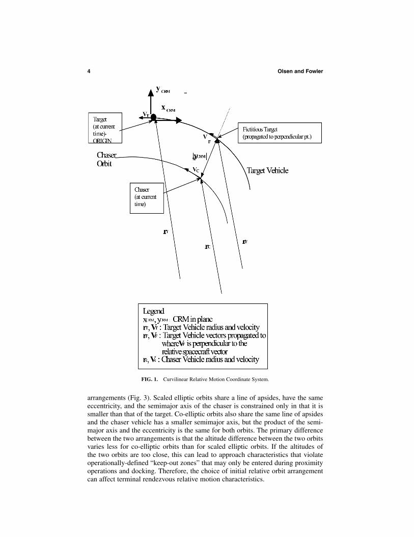
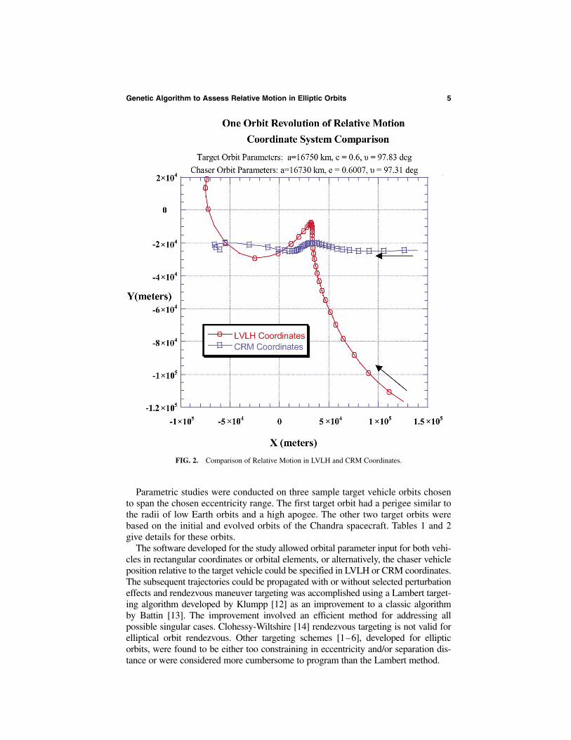
To study relative motion, one must first decide on a suitable coordinate systemin which to depict the motion. The “traditional” choice for a relative motion coor-dinate system for rendezvous studies is a target-centered, rectangular, local vertical-local horizontal (LVLH) system. The purpose of choosing a coordinate systemcentered at the target vehicle is to depict the way the motion of the chaser “looks”to the target. Merriam [10] cited the insufficiency of the rectangular LVLH systemin the case of highly elliptic orbits and presented instead a set of non-analytical,curvilinear coordinates that appeared better suited to the study of highly ellipticrendezvous, providing a truer depiction of the chaser motion relative to the target.This coordinate system is used in the current study and is called the CurvilinearRelative Motion (CRM) system.
Merriam’s CRM system is also a local set of coordinates that moves with the tar-get vehicle, but the along-track and radial components (X and Y) are calculatedthrough extrapolation of the current target vehicle position along its orbit to a pointwhere the relative vector between the two spacecraft is perpendicular to the veloc-ity vector of the target vehicle. At this point, the magnitude of the relative vector isthe magnitude of the Y coordinate. Y is defined as positive from the target vehicleaway from the Earth. The accumulated arc length that the target vehicle is “moved”to the perpendicular point is the magnitude of the X coordinate and X is defined tobe positive “behind” the target. The Z coordinate requires no special calculation. Itis the usual LVLH cross-track value. The CRM is depicted in Fig. 1. An exampleof the different character of relative motion in the LVLH and CRM systems isshown in Fig. 2. In this figure, one orbital period of relative motion between vehi-cles in neighboring, highly elliptic orbits is plotted in both sets of coordinates. Theapplication of the terms “leading vs. trailing” and “above vs. below” is different inthe two sets of coordinates. The difference is that the CRM system, being curvilin-ear, better models the curvature of the orbit than the rectangular LVLH system, andgives a more useful characterization of the relative motion. The initial semimajoraxis, eccentricity, and true anomaly of the target and chaser spacecraft are given atthe top of the figure.
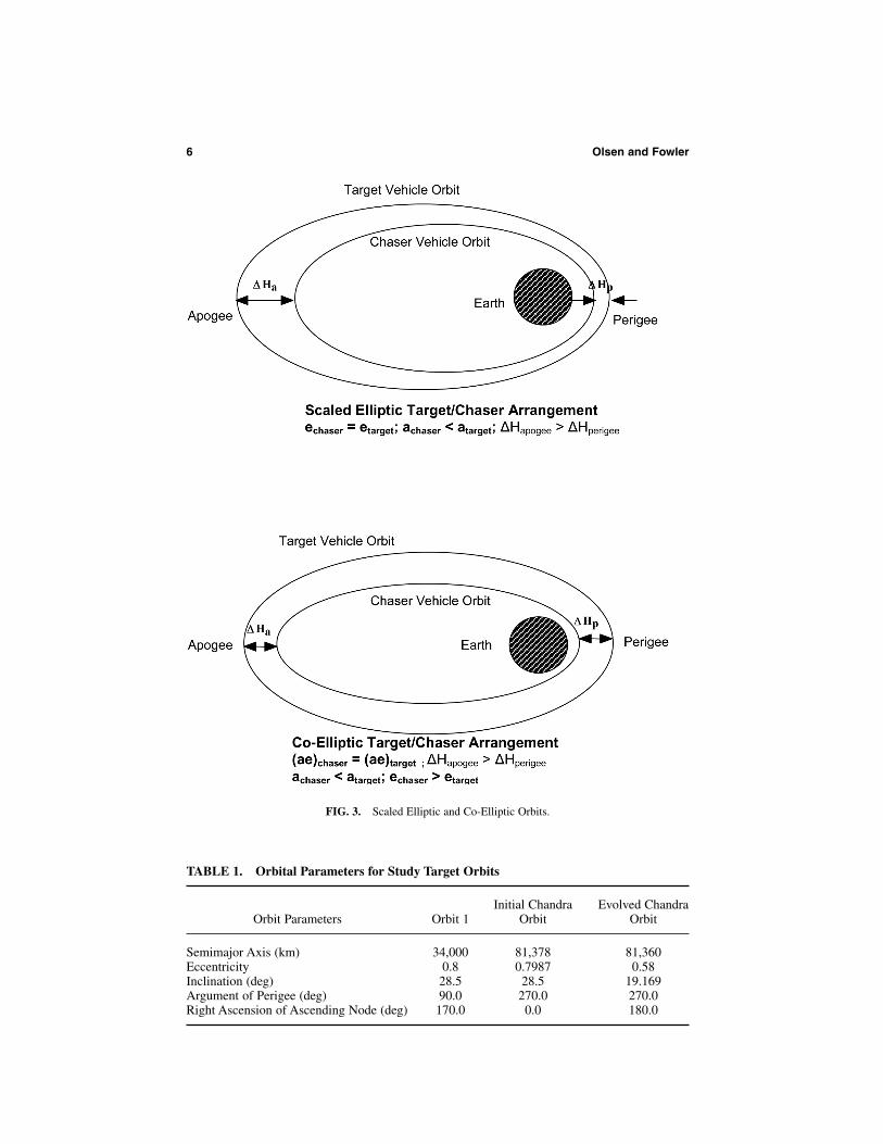
After selecting a suitable coordinate system for the relative motion, several lim-iting assumptions had to be made involving initial orbital parameters of the twovehicles in order to reduce the solution space to a manageable size. Again, follow-ing the example of the Draper research team [9–11], two target/chaser initial orbitconfigurations were chosen for use in this study: the scaled elliptic and co-elliptic
Genetic Algorithm to Assess Relative Motion in Elliptic Orbits 3
arrangements (Fig. 3). Scaled elliptic orbits share a line of apsides, have the sameeccentricity, and the semimajor axis of the chaser is constrained only in that it issmaller than that of the target. Co-elliptic orbits also share the same line of apsidesand the chaser vehicle has a smaller semimajor axis, but the product of the semi-major axis and the eccentricity is the same for both orbits. The primary differencebetween the two arrangements is that the altitude difference between the two orbitsvaries less for co-elliptic orbits than for scaled elliptic orbits. If the altitudes ofthe two orbits are too close, this can lead to approach characteristics that violateoperationally-defined “keep-out zones” that may only be entered during proximityoperations and docking. Therefore, the choice of initial relative orbit arrangementcan affect terminal rendezvous relative motion characteristics.
Parametric studies were conducted on three sample target vehicle orbits chosento span the chosen eccentricity range. The first target orbit had a perigee similar tothe radii of low Earth orbits and a high apogee. The other two target orbits werebased on the initial and evolved orbits of the Chandra spacecraft. Tables 1 and 2give details for these orbits.
The software developed for the study allowed orbital parameter input for both vehi-cles in rectangular coordinates or orbital elements, or alternatively, the chaser vehicleposition relative to the target vehicle could be specified in LVLH or CRM coordinates.The subsequent trajectories could be propagated with or without selected perturbationeffects and rendezvous maneuver targeting was accomplished using a Lambert target-ing algorithm developed by Klumpp [12] as an improvement to a classic algorithmby Battin [13]. The improvement involved an efficient method for addressing allpossible singular cases. Clohessy-Wiltshire [14] rendezvous targeting is not valid forelliptical orbit rendezvous. Other targeting schemes [1–6], developed for ellipticorbits, were found to be either too constraining in eccentricity and/or separation dis-tance or were considered more cumbersome to program than the Lambert method.
Genetic Algorithm to Assess Relative Motion in Elliptic Orbits 5
FIG. 2. Comparison of Relative Motion in LVLH and CRM Coordinates.
6 Olsen and Fowler
FIG. 3. Scaled Elliptic and Co-Elliptic Orbits.
TABLE 1. Orbital Parameters for Study Target Orbits
In early, parametric studies, rendezvous cases were run one at a time or in smallbatches with incremented transfer times. One result of these early studies was theelimination of “short” transfer times from future studies. These short times, 45 to60 minutes, are typical for circular, low-Earth orbit rendezvous transfers, but re-sult in extremely high fuel costs, and target vehicle closing rates, for highly ellip-tic cases.
Instead, it became apparent that the transfer times that characterize good ellipticrendezvous trajectories should mimic circular orbit rendezvous in that they shouldbe a similar fraction of an orbital period ( to of an orbit), although thesetransfers can be many hours in duration.
During early investigations, the effect of perturbations on targeting and propaga-tion were examined for a variety of orbits in the chosen eccentricity range. A widerange of errors, from tenths of meters to hundreds of meters, was seen in the pre-scribed final stand-off point when Lambert targeting was used, depending on theperigee height of the orbit, the transfer time, the starting and ending true anomaliesand orbit inclination. When the rendezvous occurred near perigee, the largest errorswere due to the gravity potential term of the Earth. However, even these errors wereeasily removed with one mid-course correction that constituted a 2.9% increase inthe delta-velocity of the transfer. Because of this finding, and because the earlystudies suggested the superiority of apogee rendezvous, it was decided to continuethe study without modeling perturbations.
Targeting and simulation runs were made using the target vehicle orbits in Table 1,with a chosen initial chaser vehicle position 20 km behind and 10 km below the tar-get vehicle. The desired final position was set at 1 km behind the target vehicle inthe same orbit. These values were chosen to represent “day of rendezvous” maneu-vers typical in NASA’s low Earth orbit rendezvous procedures and to stop short ofthe region labeled as proximity operations.
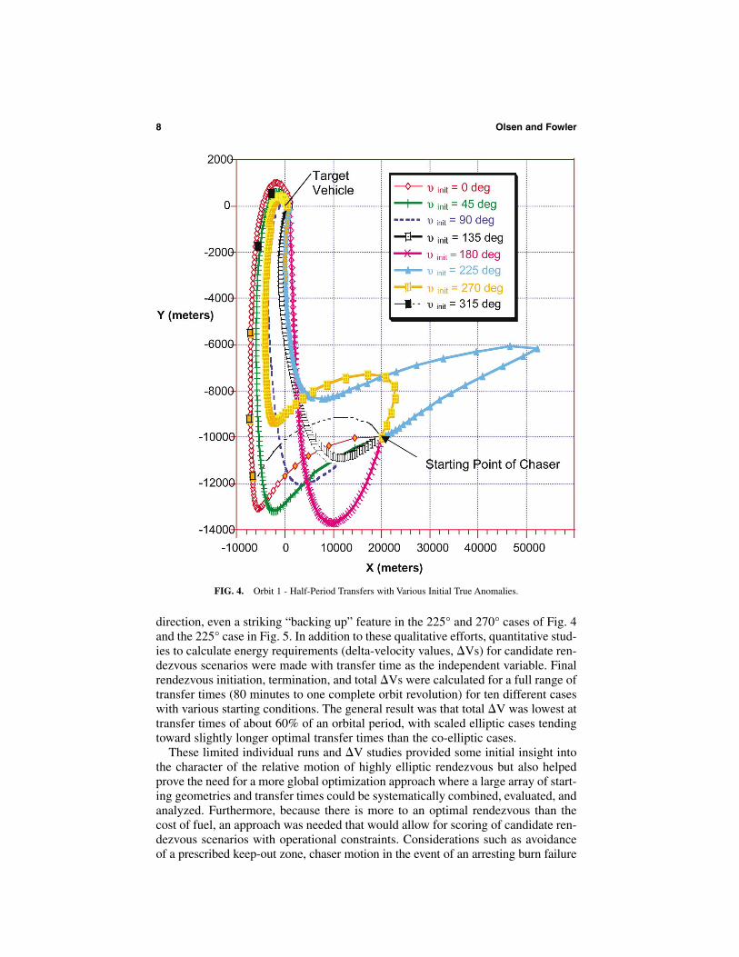
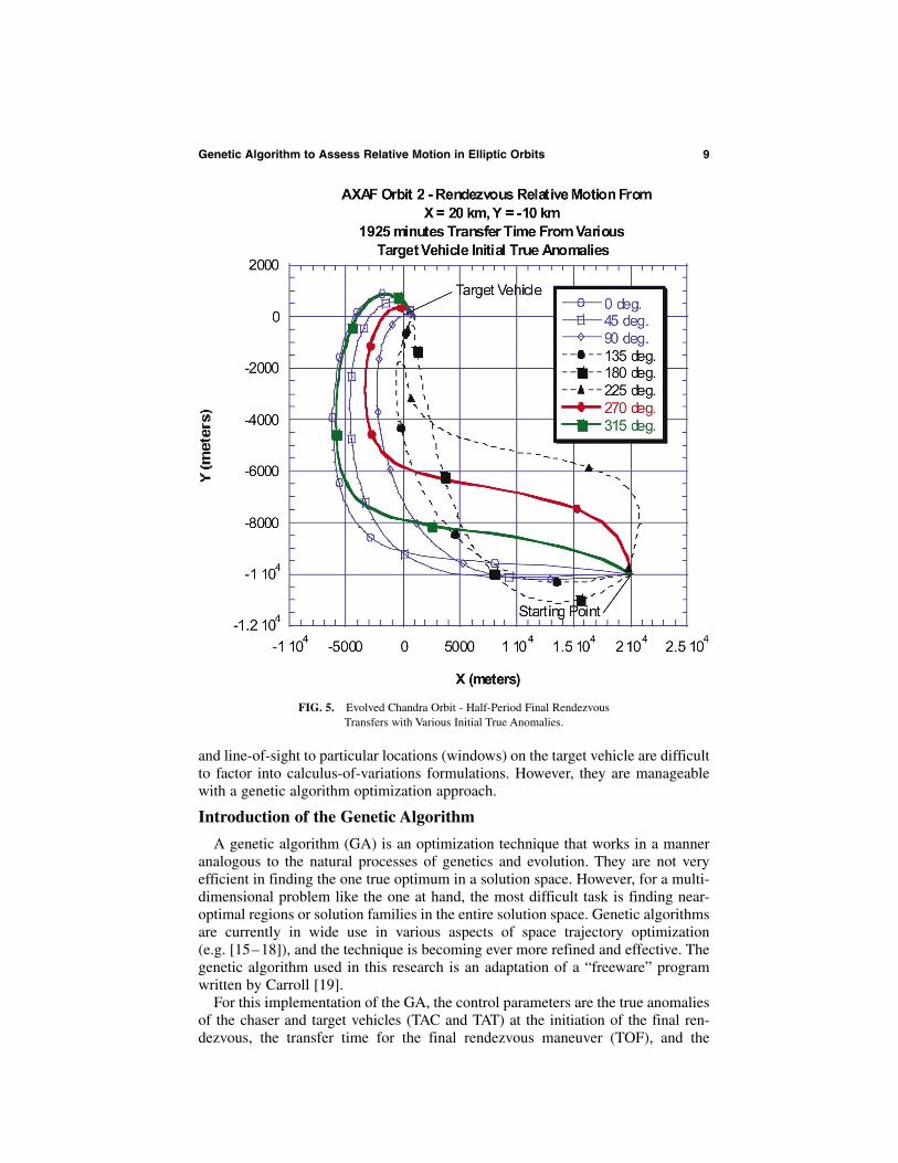
The initial true anomaly of the target vehicle was varied from 0° to 360°. Somesample results, using transfer times of half an orbital period for Orbit 1 and theevolved Chandra Orbit, are shown in Fig. 4 and Fig. 5 below. Note that the charac-ter of the relative motion changes significantly as the true anomaly is varied. Thisis more pronounced in Fig. 4, which is the case of a 0.8 eccentricity orbit, than inFig. 5, which represents a 0.58 eccentricity case. The motion seen, which agreesin character with the Draper results [9–11], is characterized by multiple changes of
J2
2�31�2
Genetic Algorithm to Assess Relative Motion in Elliptic Orbits 7
direction, even a striking “backing up” feature in the 225° and 270° cases of Fig. 4and the 225° case in Fig. 5. In addition to these qualitative efforts, quantitative stud-ies to calculate energy requirements (delta-velocity values, �Vs) for candidate ren-dezvous scenarios were made with transfer time as the independent variable. Finalrendezvous initiation, termination, and total �Vs were calculated for a full range oftransfer times (80 minutes to one complete orbit revolution) for ten different caseswith various starting conditions. The general result was that total �V was lowest attransfer times of about 60% of an orbital period, with scaled elliptic cases tendingtoward slightly longer optimal transfer times than the co-elliptic cases.
These limited individual runs and �V studies provided some initial insight intothe character of the relative motion of highly elliptic rendezvous but also helpedprove the need for a more global optimization approach where a large array of start-ing geometries and transfer times could be systematically combined, evaluated, andanalyzed. Furthermore, because there is more to an optimal rendezvous than thecost of fuel, an approach was needed that would allow for scoring of candidate ren-dezvous scenarios with operational constraints. Considerations such as avoidanceof a prescribed keep-out zone, chaser motion in the event of an arresting burn failure
8 Olsen and Fowler
FIG. 4. Orbit 1 - Half-Period Transfers with Various Initial True Anomalies.
and line-of-sight to particular locations (windows) on the target vehicle are difficultto factor into calculus-of-variations formulations. However, they are manageablewith a genetic algorithm optimization approach.
Introduction of the Genetic Algorithm
A genetic algorithm (GA) is an optimization technique that works in a manneranalogous to the natural processes of genetics and evolution. They are not veryefficient in finding the one true optimum in a solution space. However, for a multi-dimensional problem like the one at hand, the most difficult task is finding near-optimal regions or solution families in the entire solution space. Genetic algorithmsare currently in wide use in various aspects of space trajectory optimization(e.g. [15–18]), and the technique is becoming ever more refined and effective. Thegenetic algorithm used in this research is an adaptation of a “freeware” programwritten by Carroll [19].
For this implementation of the GA, the control parameters are the true anomaliesof the chaser and target vehicles (TAC and TAT) at the initiation of the final ren-dezvous, the transfer time for the final rendezvous maneuver (TOF), and the
Genetic Algorithm to Assess Relative Motion in Elliptic Orbits 9
FIG. 5. Evolved Chandra Orbit - Half-Period Final Rendezvous Transfers with Various Initial True Anomalies.
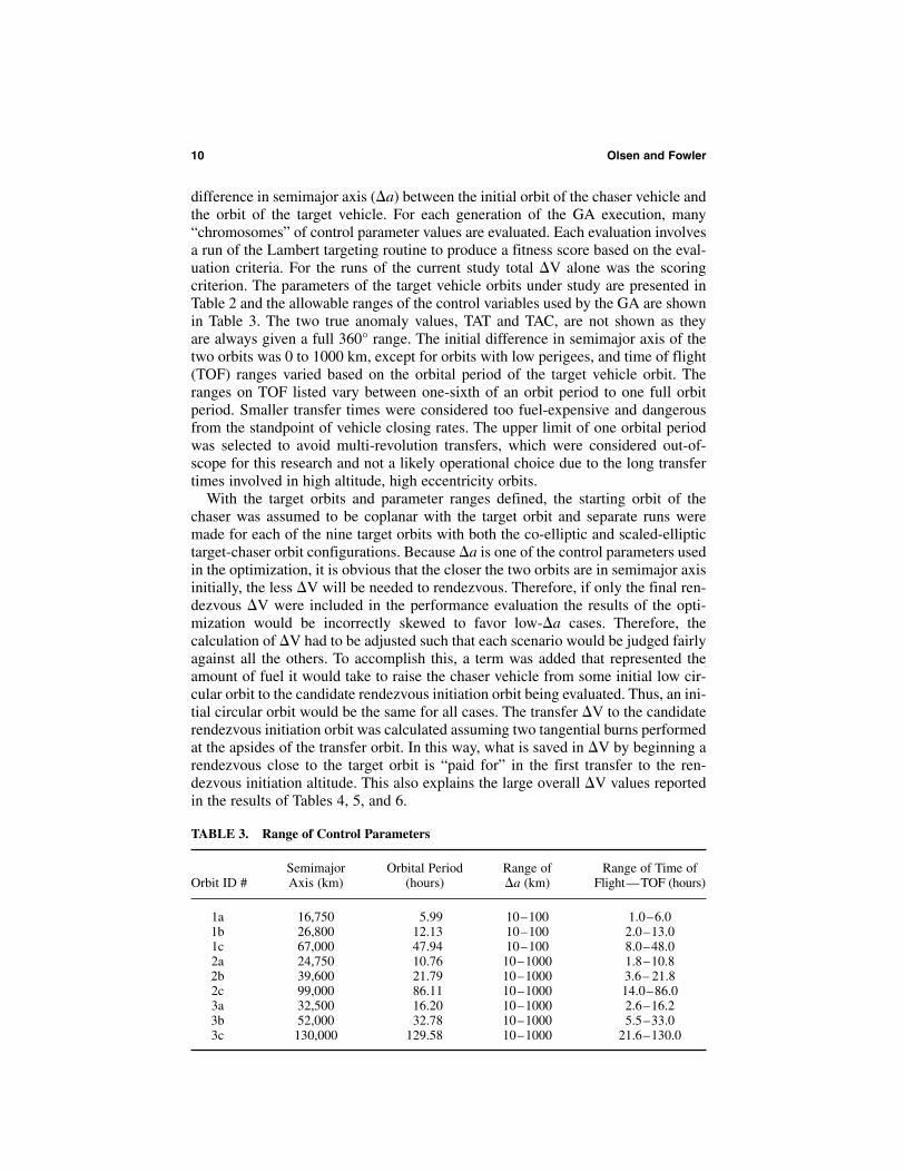
difference in semimajor axis (�a) between the initial orbit of the chaser vehicle andthe orbit of the target vehicle. For each generation of the GA execution, many“chromosomes” of control parameter values are evaluated. Each evaluation involvesa run of the Lambert targeting routine to produce a fitness score based on the eval-uation criteria. For the runs of the current study total �V alone was the scoringcriterion. The parameters of the target vehicle orbits under study are presented inTable 2 and the allowable ranges of the control variables used by the GA are shownin Table 3. The two true anomaly values, TAT and TAC, are not shown as theyare always given a full 360° range. The initial difference in semimajor axis of thetwo orbits was 0 to 1000 km, except for orbits with low perigees, and time of flight(TOF) ranges varied based on the orbital period of the target vehicle orbit. Theranges on TOF listed vary between one-sixth of an orbit period to one full orbitperiod. Smaller transfer times were considered too fuel-expensive and dangerousfrom the standpoint of vehicle closing rates. The upper limit of one orbital periodwas selected to avoid multi-revolution transfers, which were considered out-of-scope for this research and not a likely operational choice due to the long transfertimes involved in high altitude, high eccentricity orbits.
With the target orbits and parameter ranges defined, the starting orbit of thechaser was assumed to be coplanar with the target orbit and separate runs weremade for each of the nine target orbits with both the co-elliptic and scaled-elliptictarget-chaser orbit configurations. Because �a is one of the control parameters usedin the optimization, it is obvious that the closer the two orbits are in semimajor axisinitially, the less �V will be needed to rendezvous. Therefore, if only the final ren-dezvous �V were included in the performance evaluation the results of the opti-mization would be incorrectly skewed to favor low-�a cases. Therefore, thecalculation of �V had to be adjusted such that each scenario would be judged fairlyagainst all the others. To accomplish this, a term was added that represented theamount of fuel it would take to raise the chaser vehicle from some initial low cir-cular orbit to the candidate rendezvous initiation orbit being evaluated. Thus, an ini-tial circular orbit would be the same for all cases. The transfer �V to the candidaterendezvous initiation orbit was calculated assuming two tangential burns performedat the apsides of the transfer orbit. In this way, what is saved in �V by beginning arendezvous close to the target orbit is “paid for” in the first transfer to the ren-dezvous initiation altitude. This also explains the large overall �V values reportedin the results of Tables 4, 5, and 6.
10 Olsen and Fowler
TABLE 3. Range of Control Parameters
Semimajor Orbital Period Range of Range of Time of Orbit ID # Axis (km) (hours) �a (km) Flight—TOF (hours)
The process of deciding which options to use and which values to set for the var-ious inputs of a GA is often called “tuning” the algorithm. Some general guidancedoes exist, and Carroll provides some with his program. However, GA researchersgenerally admit that GA tuning can be an optimization process in its own right. TheGA used in this study does not provide an indication of convergence. The programwill run until it reaches the maximum number of generations specified. Generally,if tens of generations transpire without any change in the best function value, eitherthe program has converged to the “best” answer or the problem has been poorly for-mulated and the program will not converge. To help identify this second eventual-ity, the �V calculation for a two tangential burn transfer from the chaser orbit to thetarget orbit was made for each of the nine cases. This simple calculation was usedto determine if the minimum �V found by the GA was credible or merely the prod-uct of a poorly formulated optimization. With the GA formulation thus verified,more runs were made, with more generations, larger populations and/or differentGA parameter to see if better function values could be found.
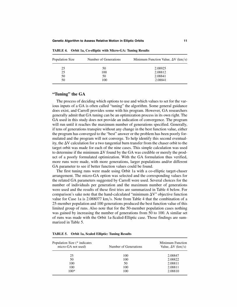
The first tuning runs were made using Orbit 1a with a co-elliptic target-chaserarrangement. The micro-GA option was selected and the corresponding values forthe related GA parameters suggested by Carroll were used. Several choices for thenumber of individuals per generation and the maximum number of generationswere used and the results of these first tries are summarized in Table 4 below. Forcomparison’s sake note that the hand-calculated “minimum �V” objective functionvalue for Case 1a is 2.088077 . Note from Table 4 that the combination of a25-member population and 100 generations produced the best function value of thislimited group of runs. Also note that for the 50-member population cases nothingwas gained by increasing the number of generations from 50 to 100. A similar setof runs was made with the Orbit 1a-Scaled-Elliptic case. Those findings are sum-marized in Table 5.
km�s
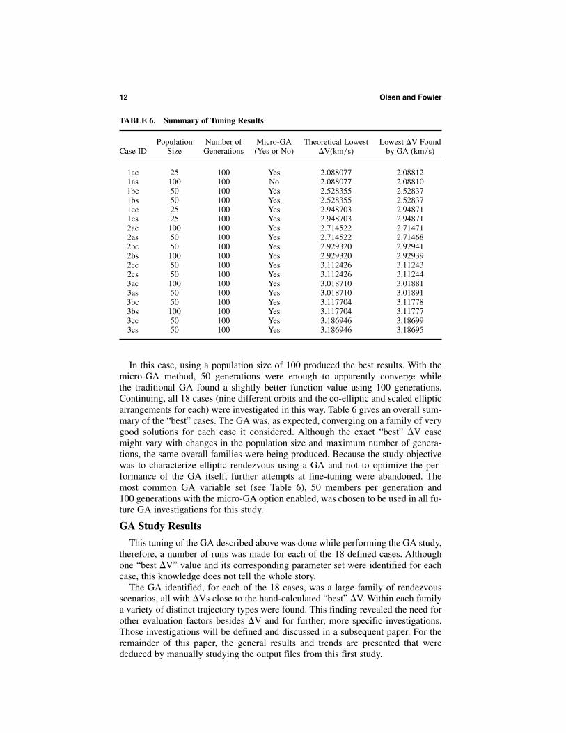
In this case, using a population size of 100 produced the best results. With themicro-GA method, 50 generations were enough to apparently converge whilethe traditional GA found a slightly better function value using 100 generations.Continuing, all 18 cases (nine different orbits and the co-elliptic and scaled ellipticarrangements for each) were investigated in this way. Table 6 gives an overall sum-mary of the “best” cases. The GA was, as expected, converging on a family of verygood solutions for each case it considered. Although the exact “best” �V casemight vary with changes in the population size and maximum number of genera-tions, the same overall families were being produced. Because the study objectivewas to characterize elliptic rendezvous using a GA and not to optimize the per-formance of the GA itself, further attempts at fine-tuning were abandoned. Themost common GA variable set (see Table 6), 50 members per generation and100 generations with the micro-GA option enabled, was chosen to be used in all fu-ture GA investigations for this study.
GA Study Results
This tuning of the GA described above was done while performing the GA study,therefore, a number of runs was made for each of the 18 defined cases. Althoughone “best �V” value and its corresponding parameter set were identified for eachcase, this knowledge does not tell the whole story.
The GA identified, for each of the 18 cases, was a large family of rendezvousscenarios, all with �Vs close to the hand-calculated “best” �V. Within each familya variety of distinct trajectory types were found. This finding revealed the need forother evaluation factors besides �V and for further, more specific investigations.Those investigations will be defined and discussed in a subsequent paper. For theremainder of this paper, the general results and trends are presented that werededuced by manually studying the output files from this first study.
12 Olsen and Fowler
TABLE 6. Summary of Tuning Results
Population Number of Micro-GA Theoretical Lowest Lowest �V Found Case ID Size Generations (Yes or No) �V( ) by GA ( )
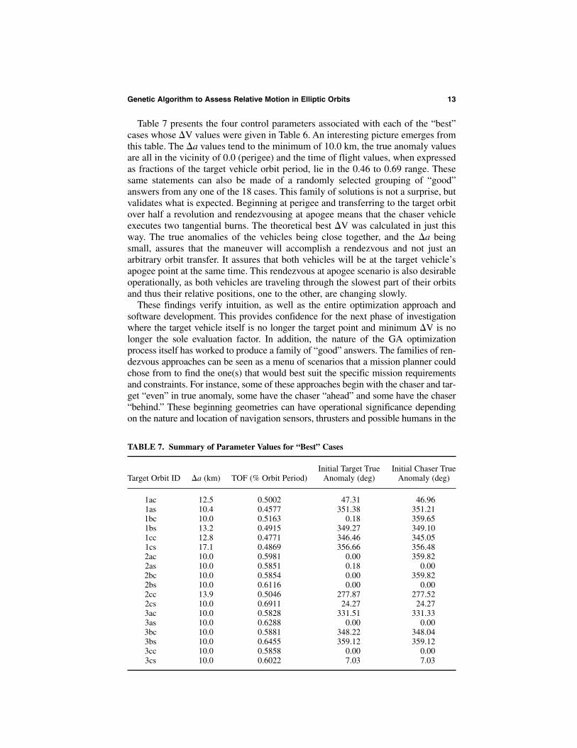
Table 7 presents the four control parameters associated with each of the “best”cases whose �V values were given in Table 6. An interesting picture emerges fromthis table. The �a values tend to the minimum of 10.0 km, the true anomaly valuesare all in the vicinity of 0.0 (perigee) and the time of flight values, when expressedas fractions of the target vehicle orbit period, lie in the 0.46 to 0.69 range. Thesesame statements can also be made of a randomly selected grouping of “good”answers from any one of the 18 cases. This family of solutions is not a surprise, butvalidates what is expected. Beginning at perigee and transferring to the target orbitover half a revolution and rendezvousing at apogee means that the chaser vehicleexecutes two tangential burns. The theoretical best �V was calculated in just thisway. The true anomalies of the vehicles being close together, and the �a beingsmall, assures that the maneuver will accomplish a rendezvous and not just anarbitrary orbit transfer. It assures that both vehicles will be at the target vehicle’sapogee point at the same time. This rendezvous at apogee scenario is also desirableoperationally, as both vehicles are traveling through the slowest part of their orbitsand thus their relative positions, one to the other, are changing slowly.
These findings verify intuition, as well as the entire optimization approach andsoftware development. This provides confidence for the next phase of investigationwhere the target vehicle itself is no longer the target point and minimum �V is nolonger the sole evaluation factor. In addition, the nature of the GA optimizationprocess itself has worked to produce a family of “good” answers. The families of ren-dezvous approaches can be seen as a menu of scenarios that a mission planner couldchose from to find the one(s) that would best suit the specific mission requirementsand constraints. For instance, some of these approaches begin with the chaser and tar-get “even” in true anomaly, some have the chaser “ahead” and some have the chaser“behind.” These beginning geometries can have operational significance dependingon the nature and location of navigation sensors, thrusters and possible humans in the
Genetic Algorithm to Assess Relative Motion in Elliptic Orbits 13
TABLE 7. Summary of Parameter Values for “Best” Cases
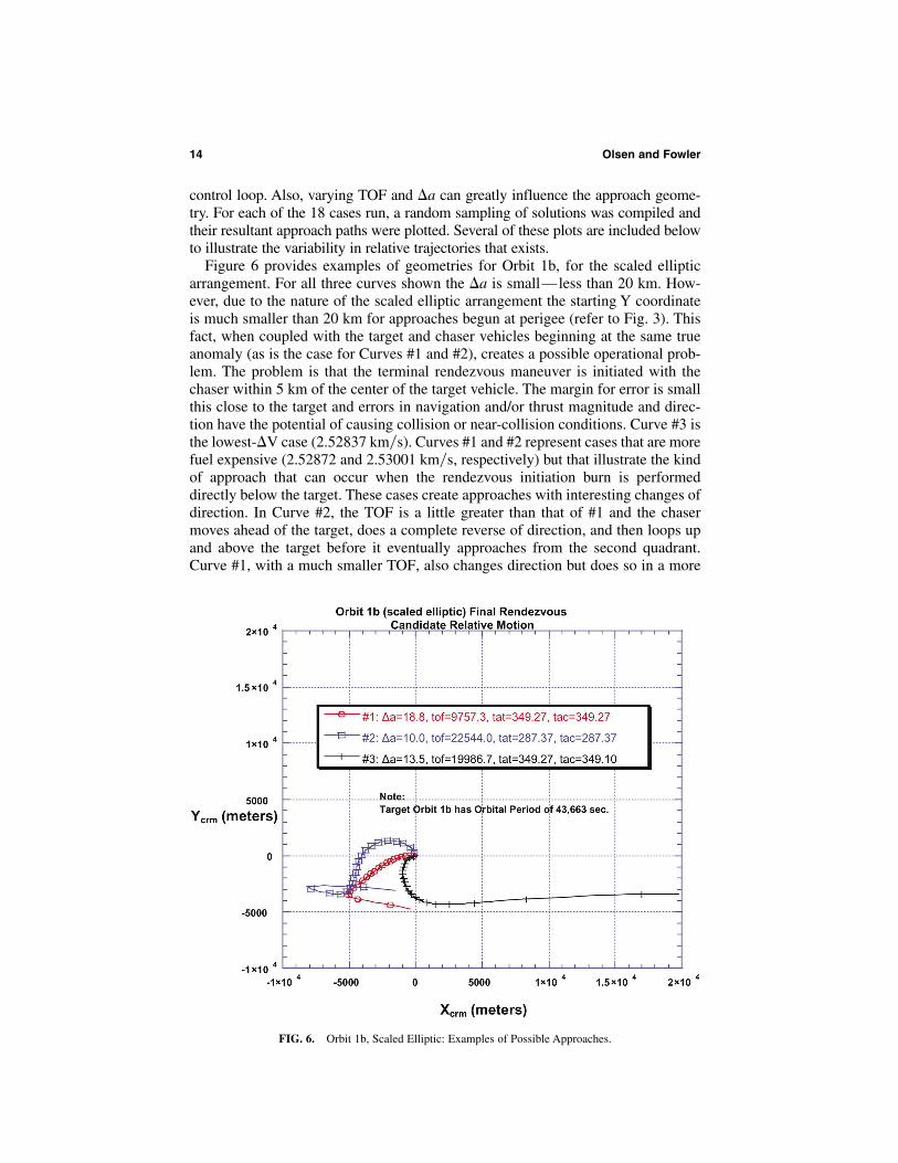
control loop. Also, varying TOF and �a can greatly influence the approach geome-try. For each of the 18 cases run, a random sampling of solutions was compiled andtheir resultant approach paths were plotted. Several of these plots are included belowto illustrate the variability in relative trajectories that exists.
Figure 6 provides examples of geometries for Orbit 1b, for the scaled ellipticarrangement. For all three curves shown the �a is small— less than 20 km. How-ever, due to the nature of the scaled elliptic arrangement the starting Y coordinateis much smaller than 20 km for approaches begun at perigee (refer to Fig. 3). Thisfact, when coupled with the target and chaser vehicles beginning at the same trueanomaly (as is the case for Curves #1 and #2), creates a possible operational prob-lem. The problem is that the terminal rendezvous maneuver is initiated with thechaser within 5 km of the center of the target vehicle. The margin for error is smallthis close to the target and errors in navigation and/or thrust magnitude and direc-tion have the potential of causing collision or near-collision conditions. Curve #3 isthe lowest-�V case (2.52837 ). Curves #1 and #2 represent cases that are morefuel expensive (2.52872 and 2.53001 , respectively) but that illustrate the kindof approach that can occur when the rendezvous initiation burn is performeddirectly below the target. These cases create approaches with interesting changes ofdirection. In Curve #2, the TOF is a little greater than that of #1 and the chasermoves ahead of the target, does a complete reverse of direction, and then loops upand above the target before it eventually approaches from the second quadrant.Curve #1, with a much smaller TOF, also changes direction but does so in a more
km�skm�s
14 Olsen and Fowler
FIG. 6. Orbit 1b, Scaled Elliptic: Examples of Possible Approaches.
abrupt manner. This curve, in its final stages, becomes an X-axis approach. In circularorbit terminology, this is referred to as a “VBAR” approach as the target vehicle’svelocity vector points along the X-axis.
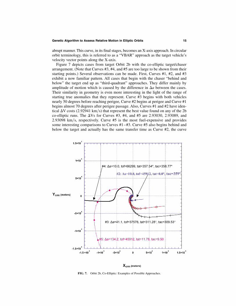
Figure 7 depicts cases from target Orbit 2b with the co-elliptic target/chaserarrangement. (Note that Curves #3, #4, and #5 are too large to be shown from theirstarting points.) Several observations can be made. First, Curves #1, #2, and #3exhibit a now familiar pattern. All cases that begin with the chaser “behind andbelow” the target end up as “third-quadrant” approaches. They differ mainly byamplitude of motion which is caused by the difference in �a between the cases.Their similarity in geometry is even more interesting in the light of the range ofstarting true anomalies that they represent. Curve #3 begins with both vehiclesnearly 50 degrees before reaching perigee, Curve #2 begins at perigee and Curve #1begins almost 70 degrees after perigee passage. Also, Curves #1 and #2 have iden-tical �V costs (2.92941 ) that represent the best value found on any of the 2bco-elliptic runs. The �Vs for Curves #3, #4, and #5 are 2.93030, 2.93089, and2.93098 respectively. Curve #5 is the most fuel-expensive and providessome interesting comparisons to Curves #1–#3. Curve #5 also begins behind andbelow the target and actually has the same transfer time as Curve #2, the curve
km�s,
km�s
Genetic Algorithm to Assess Relative Motion in Elliptic Orbits 15
FIG. 7. Orbit 2b, Co-Elliptic: Examples of Possible Approaches.
with the most “compact” geometry. The reason for the massive difference in thecurves is obvious. Curve #5 represents a case where �a is 134.2 km, as opposedto 10.0 km for Curve #2. Curve #5 has to travel a much greater distance in thesame time. Therefore, more energy must be expended and a larger, more exagger-ated curve results. Even though the general shape of Curve #5 is not unlikeCurves #1–#3 its large, exaggerated nature causes it to cross the negative X-axisand approach the target from the second quadrant. Curve #4, however, is completelydifferent. With Curve #4 the chaser vehicle begins ahead of the target in trueanomaly and at the lowest �a value of 10 km. In addition, this is a long transfertime case–0.845 of an orbit revolution in length. This combination of parameterscreates a novel relative motion curve. The chaser vehicle begins 210 km ahead ofthe target and 10 km below. The chaser then “backs up” toward the target almoston a straight line until it is only 60 km ahead of the target. It then begins a loop upacross the �X-axis and eventually to the �Y axis (RBAR) down which it travelsto the target.
Conclusion
The initial study considered 18 cases. That is, there were nine target orbit casesrun with each of the initial target-chaser geometries—co-elliptic and scaled elliptic.The final targeted position for the chaser vehicle was the target vehicle itself (i.e.,no stand-off distance specified) and the evaluation function was the total �V. Thegenetic algorithm identified for each case a large family of rendezvous scenarios,all with �Vs close to the hand-calculated “best” �V. This expected result serves tovalidate the approach and the genetic algorithm implementation.
Within each family of low-�V cases a variety of distinct trajectory types werefound. An examination of these results indicate that a “good” value for the initialdifference in the semimajor axes of the chaser and target orbits was 10 km, thatinitial true anomaly values should be near perigee (within 40 degrees), andthat “good” flight times ranged between 46% and 69% of the orbital period ofthe target orbit. These parameters produced, in general, a perigee to apogee typeof rendezvous, which is also expected, as it mimics a Hohmann-type, minimumenergy transfer.
In addition to these generalized results it is notable that a large variance in thecharacter of approach relative motion is achievable while keeping �V values near-optimal. This is encouraging from a mission planning and operations perspective.As is the case with current (Shuttle and International Space Station) rendezvousexperience, multiple viable approach scenarios are desirable in order to accommo-date the various operational constraints that are encountered, including but notlimited to navigation, lighting, and vehicle/crew safety considerations.
With the genetic algorithm method developed herein for the study of final ren-dezvous relative motion it is possible to further characterize the broad regions of“good” solutions identified. The targeted final position of the chaser can be gener-alized to any stand-off point (on the RBAR, VBAR or elsewhere) that is opera-tionally desirable. A safety zone of exclusion can easily be defined about the targetvehicle and candidate scenarios can be penalized if the zone is entered during finalrendezvous transfer or in the event of a failed arresting burn. In short, the methoddescribed above shows promise as a preliminary design tool for operationally feasiblerendezvous in highly elliptic orbit.
16 Olsen and Fowler
References[1] DeVRIES, J. P. “Elliptic Elements in Terms of Small Increments of Position and Velocity
Components,” AIAA Journal, Vol. 1, No. 11, November, 1963, pp. 2626–2629.[2] LONDON, H. S. “Second-Approximation to the Solution of the Rendezvous Equations,” AIAA
Journal, Vol. 1, 1963, pp. 1691–1693.[3] EULER, E. A. and SHULMAN, Y. “Second-Order Solution to the Elliptical Rendezvous Prob-
lem,” AIAA Journal, Volume 5, 1967.[4] GARRISON, J. L., GARDNER, T. G., and AXELRAD, P. “Relative Motion in Highly Elliptical
Orbits,” Proceedings of the AAS/AIAA Space Flight Mechanics Meeting, Paper AAS 95-194,February, 1995.
[5] KECHICHIAN, J. A. “Analysis of the Relative Motion in General Elliptic Orbit with Respectto a Dragging and Precessing Coordinate Frame,” Proceedings of the 1997 AAS/AIAA Astrody-namics Conference, Sun Valley, ID, August 4–7, 1997.
[6] TSCHAUNER, J. “Elliptic Orbit Rendezvous,” AIAA Journal, Vol. 5, No. 6, 1967, pp. 1110–1113.[7] JEZEWSKI, D. J., BRAZZELL, J. P., PRUST, E. E., BROWN, B. G., MULDER, T. A., and
WISSINGER, D. B. “A Survey of Rendezvous Trajectory Planning,” Paper AAS 92-4507,Proceedings of the AIAA/AAS Astrodynamics Conference, August, 1992.
[8] SMITH, N. G. and HONG, P. E. “Elliptic Rendezvous at Mars,” Paper AAS 91-504, Proceed-ings of the AIAA/AAS Astrodynamics Conference, August, 1991.
[9] SHEPPERD, S. “Elliptic Orbit Rendezvous, Issues and Preliminary Concerns,” PresentationMaterials Presented at NASA-JSC by the C. S. Draper Laboratory in support of the SpaceExploration Initiative, March, 1990.
[10] MERRIAM, R. S. “A Method for Computing the Relative Motion between Two Vehicles inElliptical Orbits,” NASA-JSC Memo for Record, No. ET4-92-06, February 10, 1992.
[11] LYON, J. A. “A Study of Selected Relative Motions between Two Vehicles in Highly EllipticalMars Orbits,” NASA-JSC Memo for Record, No. ET4-92-15, June 23, 1992.
[12] KLUMPP, A. R. “Universal Lambert and Kepler Algorithms for Autonomous Rendezvous,”Paper AIAA 90-2883, Proceedings of the AIAA/AAS Astrodynamics Conference, August, 1990.
[13] BATTIN, R. H. An Introduction to the Mathematics and Methods of Astrodynamics, AmericanInstitute of Aeronautics and Astronautics, Inc., New York, N. Y., 1987.
[14] CLOHESSY, W. H. and WILTSHIRE, R. S. “Terminal Guidance System for Satellite Ren-dezvous,” Journal of the Aerospace Sciences, Vol. 27, No. 9, September, 1960.
[15] PINON, III, E. An Investigation of the Applicability of Genetic Algorithms to Spacecraft Tra-jectory Optimization, Ph.D. Dissertation, University of Texas at Austin, May, 1995.
[16] HARTMANN, J. W., COVERSTONE-CARROLL, V. L., and WILLIAMS, S. N. “OptimalInterplanetary Spacecraft Trajectories via a Pareto Genetic Algorithm,” The Journal of theAstronautical Sciences, Vol. 46, July–September, 1998, pp. 267–282.
[17] KIM, Y. H. and SPENCER, D. B. “Optimal Spacecraft Rendezvous Using Genetic Algorithms,”Journal of Spacecraft and Rockets, Vol. 39, November–December, 2002, pp. 859–865.
[18] ROGATA, P., DI SOTTO, E., GRAZIANO, M., and GRAZIANI, F. “Guess Values for Inter-planetary Transfer Design Through Genetic Algorithms,” Advances in the AstronauticalSciences, Vol. 114, 2003, pp. 605–619.
[19] CARROLL, D. L. “Fortran Genetic Algorithm Driver Program Documentation,” UnpublishedListing and Explanation of Free-ware Computer Program, Version 1.6.4, University of Illinois,Champaign-Urbana, Illinois, January, 1997.
[20] OLSEN, C. D. Characterization of the Relative Motion of Rendezvous Between Vehicles inProximate, Highly Elliptic Orbits, Ph. D. Dissertation, University of Texas at Austin, May, 2001.
Genetic Algorithm to Assess Relative Motion in Elliptic Orbits 17