39
Catalogue no. 13-606-G ISBN 978-0-660-28604-4 Release date: November 30, 2016 User Guide: Canadian System of Macroeconomic Accounts Chapter 7 Price and volume measures

Catalogue no. 13-606-G ISBN 978-0-660-28604-4
Release date: November 30, 2016
User Guide: Canadian System of Macroeconomic Accounts
Chapter 7 Price and volume measures

How to obtain more informationFor information about this product or the wide range of services and data available from Statistics Canada, visit our website, www.statcan.gc.ca. You can also contact us by email at [email protected] telephone, from Monday to Friday, 8:30 a.m. to 4:30 p.m., at the following numbers:
• Statistical Information Service 1-800-263-1136 • National telecommunications device for the hearing impaired 1-800-363-7629 • Fax line 1-514-283-9350
Depository Services Program
• Inquiries line 1-800-635-7943 • Fax line 1-800-565-7757
Standards of service to the publicStatistics Canada is committed to serving its clients in a prompt, reliable and courteous manner. To this end, Statistics Canada has developed standards of service that its employees observe. To obtain a copy of these service standards, please contact Statistics Canada toll-free at 1-800-263-1136. The service standards are also published on www.statcan.gc.ca under “Contact us” > “Standards of service to the public.”
Note of appreciationCanada owes the success of its statistical system to a long-standing partnership between Statistics Canada, the citizens of Canada, its businesses, governments and other institutions. Accurate and timely statistical information could not be produced without their continued co-operation and goodwill.
This publication contains nine chapters to reflect the most of the macroeconomic accounts. Some chapters ( 1, 2, 3, 4, 6, 7 and 9) were updated on February 22, 2021 to fix some references. For more information on Satellite accounts and Natural resource accounts, please refer to Canadian System of Macroeconomic Accounts (13-607-X).
Published by authority of the Minister responsible for Statistics Canada
© Her Majesty the Queen in Right of Canada as represented by the Minister of Industry, 2019
All rights reserved. Use of this publication is governed by the Statistics Canada Open Licence Agreement.
An HTML version is also available.
Cette publication est aussi disponible en français.

Statistics Canada – Catalogue no. 13-606-G 3
User Guide: Canadian System of Macroeconomic Accounts
Table of contents
Chapter 7 Price and volume measures ................................................................................................ 4
What this chapter seeks to do.............................................................................................................. 4
7.1 Introduction .................................................................................................................................... 4
7.2 Decomposing aggregates of transaction values: the simple case ................................................. 4
7.3 Decomposing aggregates of transaction values: the more common, complex case .................... 6
7.3.1 Laspeyres, Paasche and Fisher price indexes ...................................................................... 6
7.3.2 Laspeyres, Paasche and Fisher volume indexes ........................................................................ 9
7.3.3 The value indexes ............................................................................................................... 12
7.3.4 Substitution bias and chained indexes ............................................................................... 13
7.3.5 Additivity of Laspeyres and Paasche volume indexes and double deflation ...................... 14
7.3.6 Consistency of Laspeyres, Paasche and Fisher price and volume indexes ....................... 17
7.3.7 Elementary versus compound price and volume indexes .................................................. 19
7.3.8 Contributions to change ...................................................................................................... 21
7.4 Index number calculations in the national accounts .................................................................... 23
7.4.1 Price deflation versus direct volume measurement ............................................................ 23
7.4.2 Income and expenditure accounts deflation ....................................................................... 24
7.4.3 Supply and use accounts deflation ..................................................................................... 25
7.5 Deflation of stocks ........................................................................................................................ 25
7.5.1 Fixed capital stocks ............................................................................................................ 25
7.5.2 Inventory stocks .................................................................................................................. 27
7.6 Real gross domestic income and the terms of trade ................................................................... 28
7.7 Inter-regional price and volume indexes ...................................................................................... 29
7.7.1 Purchasing power parities ................................................................................................... 29
7.7.2 Real income comparisons across regions .......................................................................... 31
Annex A.7.1 Price indexes produced by Statistics Canada ............................................................... 32
Annex A.7.1.1 Consumer price indexes ....................................................................................... 33
Annex A.7.1.2 Industrial product price indexes ........................................................................... 33
Annex A.7.1.3 Machinery and equipment price indexes .............................................................. 34
Annex A.7.1.4 Agriculture price indexes ...................................................................................... 34
Annex A.7.1.5 Construction price indexes ................................................................................... 34
Annex A.7.1.6 Services producer price indexes .......................................................................... 35
Annex A.7.1.7 International merchandise trade price indexes ..................................................... 35
Notes for chapter 7 .............................................................................................................................. 37

Statistics Canada – Catalogue no. 13-606-G4
User Guide: Canadian System of Macroeconomic Accounts
User Guide: Canadian System of Macroeconomic Accounts
Chapter 7 Price and volume measures
What this chapter seeks to do
This chapter explains how the various time series in the national accounts pertaining to expenditures on goods and services, including expenditures on industry inputs and outputs, are decomposed into distinct ‘price’ and ‘volume’ components. It also discusses how these decompositions are used in practice. In addition, the chapter looks at a number of ‘real income’ concepts. Ending the chapter is a section on international price and volume comparisons.
This chapter links to SNA 2008 chapter 15.
7.1 Introduction
The national accounts are mostly about aggregates of transaction values and stocks of assets and liabilities. Some transaction aggregates, such as ‘household final expenditure on consumer goods and services’, are about goods and services and can be decomposed into price and volume1 components. Others, such as ‘current transfers from government to non-residents’, are not, although changes in their associated purchasing power can be gauged with the use of price indexes. An individual transaction value pertaining to a specific good or service is obtained by multiplying the price of the product by the quantity of the product that is purchased/sold in that transaction. An aggregate of several transaction values is calculated by summing the individual values of those transactions. An aggregate of stock time series is derived similarly by adding the individual stock series together.
The decomposition of value time series into price and volume components is a very important aspect in national accounting. It makes possible the analysis of ‘real growth’, ‘productivity change’ and ‘inflation’. Imagine, for example, that the value of gross domestic product per capita, in nominal terms, increased 20 per cent over the course of a decade. That might seem like a huge jump in living standards, but if the price-volume decomposition indicated that price increases accounted for 16 per cent of the rise and volume changes accounted for just 4 per cent of the advance, then the improvement in living standards would really be more modest. Most of the change over the decade would be attributable to inflation.
The price-volume decomposition allows users of the national accounts to ‘draw back the veil of inflation’ to determine what is happening in the ‘real’ economy. Price indexes permit analyses of relative price changes, which are the most basic signals provided by the free market economy as to how resources are being reallocated to meet the highest priority needs, while volume indexes show how the different components of the economy are expanding or shrinking as a result.
This chapter is mainly about the various ways in which changes in aggregates of transactions in diverse products can be decomposed into distinct price and volume components. In section 7.2, section 7.3 and section 7.4 the Laspeyres, Paasche and Fisher price-volume decompositions are explained in some detail, from both the theoretical and the practical perspectives. Section 7.5 considers the problem of constructing a stock time series with consistent value, volume and price components. In section 7.6 a number of ‘real income’ concepts are introduced. Purchasing power parities and international income comparisons are the topic of section 7.7. An annex closes out the chapter, reviewing the various sets of price indexes that are available from Statistics Canada.
7.2 Decomposing aggregates of transaction values: the simple case
If all the individual transactions in a particular aggregate of transactions pertain to an identical product, but with different prices and quantities, the price-volume decomposition is straightforward. Since the products involved in the transactions are identical, the aggregate volume for all of the transactions can be calculated as the sum of the individual quantities purchased/sold in each transaction. The aggregate price can be calculated as a weighted average of the prices in each of the individual transactions, with the quantities of each transaction serving as the weights. Equivalently, the aggregate price can also be calculated as the aggregate transaction value divided by the aggregate transaction volume. This logic is encapsulated in equations (7.1) to (7.5) below.

Statistics Canada – Catalogue no. 13-606-G 5
User Guide: Canadian System of Macroeconomic Accounts
The value associated with an individual transaction i (𝑣𝑣𝑖𝑖) is the product of the price of that transaction ( 𝑝𝑝𝑖𝑖 ) and the quantity of that transaction (𝑞𝑞𝑖𝑖):
(7.1)
𝑣𝑣𝑖𝑖 = 𝑝𝑝𝑖𝑖 𝑞𝑞𝑖𝑖
The aggregate value for several transactions(𝑉𝑉 ) in an identical product involving different prices and quantities for each transaction is the sum of the values for all of the transactions in the aggregate:
(7.2)
�̅�𝑉 =∑𝑣𝑣𝑖𝑖 =∑𝑝𝑝𝑖𝑖 𝑞𝑞𝑖𝑖
The aggregate volume (or quantity) for several transactions (𝑄𝑄 ) in an identical product involving different prices and quantities for each transaction is the sum of the quantities for all the transactions in the aggregate:
(7.3)
𝑄𝑄 = ∑ 𝑞𝑞𝑖𝑖
The aggregate price for several transactions (𝑃𝑃 ) in an identical product involving different prices and quantities for each transaction is the aggregate value divided by the aggregate volume, or equivalently the weighted average price over all the transactions with the weights being the quantities transacted:
(7.4)
�̅�𝑃 = �̅�𝑉�̅�𝑄 =
∑𝑝𝑝𝑖𝑖𝑞𝑞𝑖𝑖∑ 𝑞𝑞𝑖𝑖
=∑𝑝𝑝𝑖𝑖 (𝑞𝑞𝑖𝑖∑𝑞𝑞𝑖𝑖
)
Accordingly, the price-volume decomposition is:
(7.5)
𝑉𝑉 = 𝑃𝑃 × 𝑄𝑄
This is the simple case, but it is not the one that is usually dealt with in national accounting. The norm, rather, is that the products involved in an aggregate of several transactions are not identical. Thus, for example, the aggregate ‘household final expenditure on consumer goods and services’ includes transactions for a very wide range of different products—food items, clothing items, manufactured goods, personal services and so on. In this circumstance, the quantity involved in one transaction (number of cars, for example) is unlikely to be commensurable2 with that of another transaction (kilograms of bananas, for example). Price and volume index numbers are needed to deal with non-commensurable cases such as this. They deal with the issue of non-commensurability by addressing relative changes in prices and volumes, rather than the prices and volumes themselves.
Statistics Canada – Catalogue no. 13-606-G6
User Guide: Canadian System of Macroeconomic Accounts
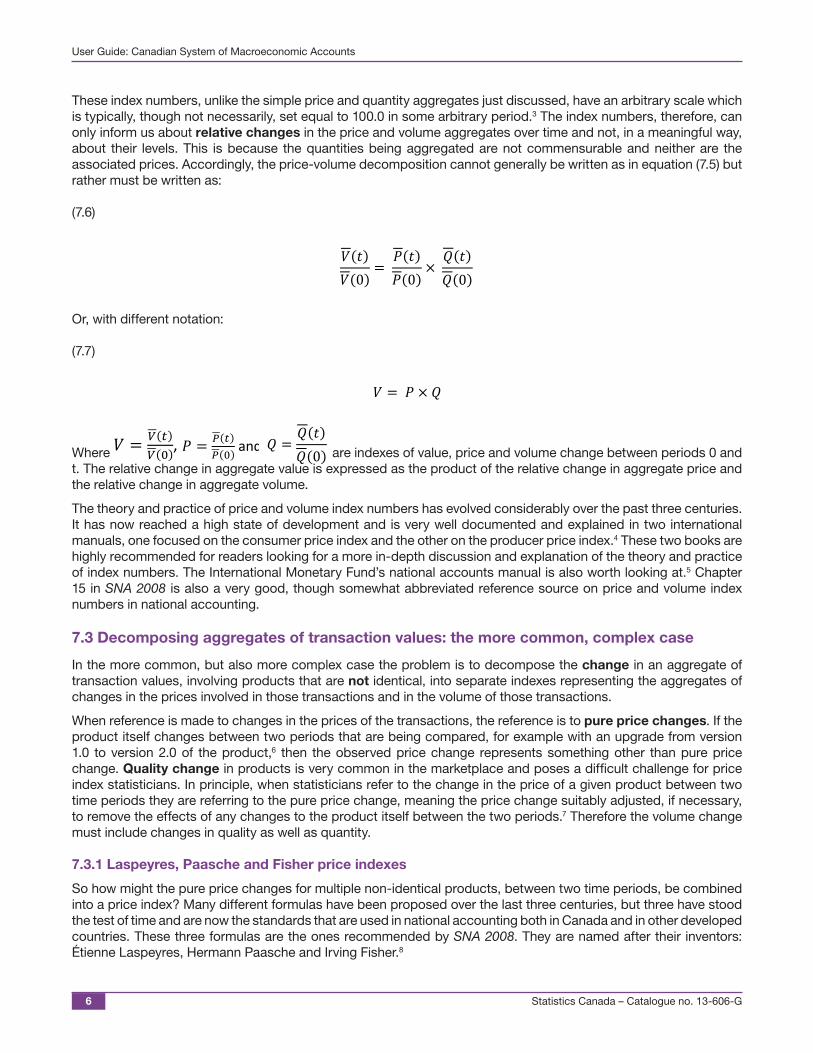
These index numbers, unlike the simple price and quantity aggregates just discussed, have an arbitrary scale which is typically, though not necessarily, set equal to 100.0 in some arbitrary period.3 The index numbers, therefore, can only inform us about relative changes in the price and volume aggregates over time and not, in a meaningful way, about their levels. This is because the quantities being aggregated are not commensurable and neither are the associated prices. Accordingly, the price-volume decomposition cannot generally be written as in equation (7.5) but rather must be written as:
(7.6)
𝑉𝑉(𝑡𝑡)𝑉𝑉(0)
= 𝑃𝑃(𝑡𝑡)𝑃𝑃(0)
× 𝑄𝑄(𝑡𝑡)𝑄𝑄(0)
Or, with different notation:
(7.7)
𝑉𝑉 = 𝑃𝑃 × 𝑄𝑄
Where 𝑉𝑉 𝑉 𝑉𝑉(𝑡𝑡)𝑉𝑉(0), 𝑃𝑃 𝑃 𝑃𝑃(𝑡𝑡)
𝑃𝑃(0) and 𝑄𝑄 = 𝑄𝑄(𝑡𝑡)𝑄𝑄(0)
are indexes of value, price and volume change between periods 0 and
t. The relative change in aggregate value is expressed as the product of the relative change in aggregate price and the relative change in aggregate volume.
The theory and practice of price and volume index numbers has evolved considerably over the past three centuries. It has now reached a high state of development and is very well documented and explained in two international manuals, one focused on the consumer price index and the other on the producer price index.4 These two books are highly recommended for readers looking for a more in-depth discussion and explanation of the theory and practice of index numbers. The International Monetary Fund’s national accounts manual is also worth looking at.5 Chapter 15 in SNA 2008 is also a very good, though somewhat abbreviated reference source on price and volume index numbers in national accounting.
7.3 Decomposing aggregates of transaction values: the more common, complex case
In the more common, but also more complex case the problem is to decompose the change in an aggregate of transaction values, involving products that are not identical, into separate indexes representing the aggregates of changes in the prices involved in those transactions and in the volume of those transactions.
When reference is made to changes in the prices of the transactions, the reference is to pure price changes. If the product itself changes between two periods that are being compared, for example with an upgrade from version 1.0 to version 2.0 of the product,6 then the observed price change represents something other than pure price change. Quality change in products is very common in the marketplace and poses a difficult challenge for price index statisticians. In principle, when statisticians refer to the change in the price of a given product between two time periods they are referring to the pure price change, meaning the price change suitably adjusted, if necessary, to remove the effects of any changes to the product itself between the two periods.7 Therefore the volume change must include changes in quality as well as quantity.
7.3.1 Laspeyres, Paasche and Fisher price indexes
So how might the pure price changes for multiple non-identical products, between two time periods, be combined into a price index? Many different formulas have been proposed over the last three centuries, but three have stood the test of time and are now the standards that are used in national accounting both in Canada and in other developed countries. These three formulas are the ones recommended by SNA 2008. They are named after their inventors: Étienne Laspeyres, Hermann Paasche and Irving Fisher.8

Statistics Canada – Catalogue no. 13-606-G 7
User Guide: Canadian System of Macroeconomic Accounts
The Laspeyres formula is perhaps the most intuitive of the three. It has become known as the fixed-basket approach. One imagines a basket containing the purchased quantities, in the initial period, of all the various goods and services that are to be included in the price index. These purchased quantities are multiplied by their corresponding prices, also from the initial period, to calculate the aggregate transaction value of the basket in the initial period. Then, for the second of the two periods being compared one takes the same basket of products, with the same qualities and quantities as in the initial period, and multiplies them by the corresponding prices of the second period. In effect, a hypothetical aggregate transaction value is calculated in which the quantities are the same as those in the initial period but the prices are those of the second period. The ratio of this second, hypothetical aggregate transaction value to the initial one is called the Laspeyres price index. It measures the relative change in the cost of the fixed initial basket of quantities between the first and second periods.
The Laspeyres price index can be written mathematically as in equation (7.8):
(7.8)
𝑃𝑃𝐿𝐿 =∑𝑝𝑝𝑖𝑖(𝑡𝑡)𝑞𝑞𝑖𝑖(0)∑𝑝𝑝𝑖𝑖(0)𝑞𝑞𝑖𝑖(0)
Where 𝑃𝑃𝐿𝐿 is the Laspeyres price index,9 𝑝𝑝𝑖𝑖(0) and 𝑝𝑝𝑖𝑖(𝑡𝑡) are the prices of product i in periods 0 and t, and 𝑞𝑞𝑖𝑖(0) is the quantity of product i in period 0. Both summations are over all the products i that are included in the price index.10,11 The quantities 𝑞𝑞𝑖𝑖(0) are those constituting the fixed basket.
The index compares prices in period 0, where the index is 1, with prices in period t, where the index is 𝑃𝑃𝐿𝐿 . Often the index is multiplied by 100 so it equals that value in period 0 and 100 *𝑃𝑃𝐿𝐿 in period t. Refer to the example in text boxes 7.1 and 7.2.
Text box 7.1 Fruit example
Below are some hypothetical data that are used in the subsequent examples to illustrate the calculation of price and volume indexes. The data record the prices of apples, oranges and bananas in two time periods, labelled 0 and 1. The price is measured in dollars per kilogram and the quantity is measured in kilograms. The value is the price multiplied by the quantity and is measured in dollars. These data could pertain to a day’s worth of sales by a small fruit stand, for example.
Apples Oranges Bananas
Period 0Price (dollars per kg) 1.50 1.00 1.10Quantity (kg) 10 20 25Value (dollars) 15.00 20.00 27.50
Period 1Price (dollars per kg) 1.75 1.05 1.60Quantity (kg) 15 40 20Value (dollars) 26.25 42.00 32.00

Statistics Canada – Catalogue no. 13-606-G8
User Guide: Canadian System of Macroeconomic Accounts
Text box 7.2 Laspeyres price index example
Below is an illustration of the calculation of the Laspeyres price index, using the example data shown in text box 7.1.
Laspeyres price index comparing period 1 to period 0 = 100.0:
𝑃𝑃𝐿𝐿 = 100 × $1.75 × 10 + $1.05 × 20 + $1.60 × 25$1.50 × 10 + $1.00 × 20 + $1.10 × 25 = 125.6
The Paasche price index is the obvious alternative to the Laspeyres price index. Instead of using the quantities from the initial period, 𝑞𝑞𝑖𝑖(0) , to construct the fixed basket, the quantities from the second period, 𝑞𝑞𝑖𝑖(𝑡𝑡) , are used instead. Thus, the Paasche price index can be written mathematically as in equation (7.9):
(7.9)
𝑃𝑃𝑃𝑃 =∑𝑝𝑝𝑖𝑖(𝑡𝑡)𝑞𝑞𝑖𝑖(𝑡𝑡)∑ 𝑝𝑝𝑖𝑖(0)𝑞𝑞𝑖𝑖(𝑡𝑡)
Where 𝑃𝑃𝑃𝑃 is the Paasche price index, 𝑝𝑝𝑖𝑖(0) and 𝑝𝑝𝑖𝑖(𝑡𝑡) are the prices of product i in periods 0 and t, and 𝑞𝑞𝑖𝑖(𝑡𝑡) is the quantity of product i in period t. The Paasche price index is, in a sense, a backward-looking index since it compares the actual value of the aggregate of transactions in the second period with the hypothetical value of the aggregate of transactions in the first period wherein the prices come from the initial period but the quantities are from the second period.12 See the example in text box 7.3.
Text box 7.3 Paasche price index example
Below is an illustration of the calculation of the Paasche price index, using the example data shown in text box 7.1.
Paasche price index comparing period 1 to period 0 = 100.0:
𝑃𝑃𝑃𝑃 = 100 × $1.75 × 15 + $1.05 × 40 + $1.60 × 20$1.50 × 15 + $1.00 × 40 + $1.10 × 20 = 118.6
To complete the picture, the Fisher price index is simply the geometric average of the Laspeyres and Paasche price indexes.13 It therefore lies midway between the two.
(7.10)
𝑃𝑃𝐹𝐹 = √𝑃𝑃𝐿𝐿𝑃𝑃𝑃𝑃 = √∑ 𝑝𝑝𝑖𝑖(𝑡𝑡)𝑞𝑞𝑖𝑖(0)∑ 𝑝𝑝𝑖𝑖(0)𝑞𝑞𝑖𝑖(0) ×
∑ 𝑝𝑝𝑖𝑖(𝑡𝑡)𝑞𝑞𝑖𝑖(𝑡𝑡)∑ 𝑝𝑝𝑖𝑖(0)𝑞𝑞𝑖𝑖(𝑡𝑡)

Statistics Canada – Catalogue no. 13-606-G 9
User Guide: Canadian System of Macroeconomic Accounts
See the example in text box 7.4.
Text box 7.4 Fisher price index example
Below is an illustration of the calculation of the Fisher price index, using the example data shown in text box 7.1 and the results calculated in text boxes 7.2 and 7.3.
Fisher price index comparing period 1 to period 0 = 100.0:
𝑃𝑃𝐹𝐹 = 100 × (1.256 × 1.186)1/2 = 122.1
Fisher considered his price index formula to be an ideal blend of the best features of the Laspeyres and Paasche price indexes and modern index number statisticians generally agree with him. Diewert showed the Fisher formula to be a member of a small class of index numbers that he dubbed superlative.14
It can be shown that under certain assumptions the Laspeyres index is an upper bound on the true index while the Paasche index is a lower bound. The Fisher index, lying between the other two indexes, is the best measure of the change (again, under certain assumptions). Text box 7.5 compares the three indexes calculated in text boxes 7.2, 7.3 and 7.4.
Text box 7.5 Comparing the Laspeyres, Paasche and Fisher price indexes
The table below compares the three price indexes calculated in text boxes 7.2, 7.3 and 7.4. Note that the Fisher price index lies midway between the other two indexes. The Laspeyres index is the largest and the Paasche index is the smallest which is true in most, but not all real-world cases.
Period 0 Period 1index
Laspeyres P 100.0 125.6Paasche P 100.0 118.6Fisher P 100.0 122.1
7.3.2 Laspeyres, Paasche and Fisher volume indexes
Many Canadians are acquainted with price indexes, such as the consumer price index. However, there is less familiarity with quantity or volume indexes. They are perhaps best illustrated by real gross domestic product, which shows the trend in total economic activity after the effects of price inflation (or deflation) have been removed.
To introduce the concept, consider a family doing its weekly grocery shopping. It buys several different items in week one and pays $100. It buys different quantities of these same products, at different prices, in week two and pays $110. Some of the 10% increase in the grocery bill is due to price changes and the rest is attributable to quantity changes. The part that is due to price changes is described by a price index and the portion attributable to changes in the quantities is measured with a quantity or volume index.
What is the difference between a quantity index and a volume index? For many purposes they are the same thing, but the difference in principle is that volume indexes include the effects of quality change as well as quantity change (recall the discussion at the beginning of section 7.3). For example, a litre of high-test gasoline has higher quality than a litre of regular gasoline. The quantities purchased in two different periods might be the same, 40 litres for example, but if the product qualities differ then a volume index would take that into account as well as the quantity difference. This is accomplished by quality adjusting the observed quantities. The challenge of quality
Statistics Canada – Catalogue no. 13-606-G10
User Guide: Canadian System of Macroeconomic Accounts
adjustment is especially formidable for high-tech products such as computers and automobiles for which quality changes in numerous and complex ways every year. In what follows, all references to quantities should be interpreted as quality-adjusted quantities. References to prices should be interpreted as pure prices, with the effects of quality change removed.
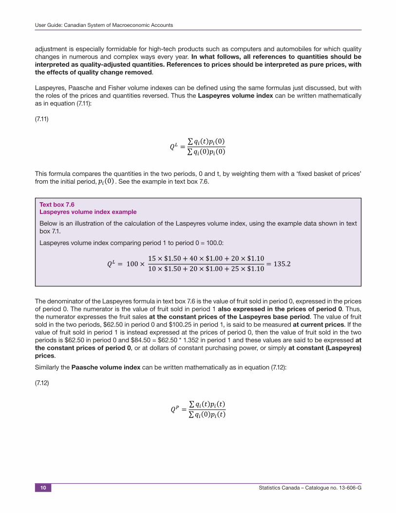
Laspeyres, Paasche and Fisher volume indexes can be defined using the same formulas just discussed, but with the roles of the prices and quantities reversed. Thus the Laspeyres volume index can be written mathematically as in equation (7.11):
(7.11)
𝑄𝑄𝐿𝐿 =∑𝑞𝑞𝑖𝑖(𝑡𝑡)𝑝𝑝𝑖𝑖(0)∑𝑞𝑞𝑖𝑖(0)𝑝𝑝𝑖𝑖(0)
This formula compares the quantities in the two periods, 0 and t, by weighting them with a ‘fixed basket of prices’ from the initial period, 𝑝𝑝𝑖𝑖(0) . See the example in text box 7.6.
Text box 7.6 Laspeyres volume index example
Below is an illustration of the calculation of the Laspeyres volume index, using the example data shown in text box 7.1.
Laspeyres volume index comparing period 1 to period 0 = 100.0:
𝑄𝑄𝐿𝐿 = 100 × 15 × $1.50 + 40 × $1.00 + 20 × $1.1010 × $1.50 + 20 × $1.00 + 25 × $1.10 = 135.2
The denominator of the Laspeyres formula in text box 7.6 is the value of fruit sold in period 0, expressed in the prices of period 0. The numerator is the value of fruit sold in period 1 also expressed in the prices of period 0. Thus, the numerator expresses the fruit sales at the constant prices of the Laspeyres base period. The value of fruit sold in the two periods, $62.50 in period 0 and $100.25 in period 1, is said to be measured at current prices. If the value of fruit sold in period 1 is instead expressed at the prices of period 0, then the value of fruit sold in the two periods is $62.50 in period 0 and $84.50 = $62.50 * 1.352 in period 1 and these values are said to be expressed at the constant prices of period 0, or at dollars of constant purchasing power, or simply at constant (Laspeyres) prices.
Similarly the Paasche volume index can be written mathematically as in equation (7.12):
(7.12)
𝑄𝑄𝑃𝑃 =∑𝑞𝑞𝑖𝑖(𝑡𝑡)𝑝𝑝𝑖𝑖(𝑡𝑡)∑𝑞𝑞𝑖𝑖(0)𝑝𝑝𝑖𝑖(𝑡𝑡)

Statistics Canada – Catalogue no. 13-606-G 11
User Guide: Canadian System of Macroeconomic Accounts
It compares the quantities in the two periods, 0 and t, by weighting them with a ‘fixed basket of prices’ from the second period, 𝑝𝑝𝑖𝑖(𝑡𝑡) . See the example in text box 7.7.
Text box 7.7 Paasche volume index example
Below is an illustration of the calculation of the Paasche volume index, using the example data shown in text box 7.1.
Paasche volume index comparing period 1 to period 0 = 100.0:
𝑄𝑄𝑃𝑃 = 100 × 15 × $1.75 + 40 × $1.05 + 20 × $1.6010 × $1.75 + 20 × $1.05 + 25 × $1.60 = 127.7
The numerator of the Paasche formula in text box 7.7 is the value of fruit sold in period 1, expressed in the prices of period 1. The denominator is the value of fruit sold in period 0 also expressed in the prices of period 1. Thus, the denominator expresses the fruit sales at the constant prices of the Paasche base period. As noted previously, the value of fruit sold in the two periods, $62.50 in period 0 and $100.25 in period 1, is said to be measured at current prices. If the value of fruit sold in period 0 is instead expressed at the prices of period 1, then the value of fruit sold in the two periods is $78.50 = $100.25/1.277 in period 0 and $100.25 in period 1 and these values are said to be expressed at the constant prices of period 1, or at dollars of constant purchasing power, or simply at constant (Paasche) prices.
The Fisher volume index, similar to its price index counterpart, is the geometric average of the Laspeyres and Paasche volume indexes.
(7.13)
𝑄𝑄𝐹𝐹 = √𝑄𝑄𝐿𝐿𝑄𝑄𝑃𝑃 = √∑ 𝑞𝑞𝑖𝑖(𝑡𝑡)𝑝𝑝𝑖𝑖(0)∑ 𝑞𝑞𝑖𝑖(0)𝑝𝑝𝑖𝑖(0) ×
∑ 𝑞𝑞𝑖𝑖(𝑡𝑡)𝑝𝑝𝑖𝑖(𝑡𝑡)∑ 𝑞𝑞𝑖𝑖(0)𝑝𝑝𝑖𝑖(𝑡𝑡)
See the example in text box 7.8.
Text box 7.8 Fisher volume index example
Below is an illustration of the calculation of the Fisher volume index, using the example data shown in text box 7.1 and the results calculated in text boxes 7.6 and 7.7.
Fisher price index comparing period 1 to period 0 = 100.0:
𝑄𝑄𝐹𝐹 = 100 × √1.352 × 1.277 = 131.4
Fisher volume indexes do not have the intuitive “at constant prices” interpretation that was discussed previously for the Laspeyres and Paasche volume indexes.

Statistics Canada – Catalogue no. 13-606-G12
User Guide: Canadian System of Macroeconomic Accounts
Text box 7.9 Comparing the Laspeyres, Paasche and Fisher volume indexes
The table below compares the three volume indexes calculated in text boxes 7.6, 7.7 and 7.8. Note that the Fisher volume index lies midway between the other two indexes. The Laspeyres index is the largest and the Paasche index is the smallest which is true in most, but not all real-world cases.
Period 0 Period 1index
Laspeyres Q 100.0 135.2Paasche Q 100.0 127.7Fisher Q 100.0 131.4
7.3.3 The value indexes
It is not difficult to prove mathematically that the product of the Fisher price and volume indexes is the value index, V (that is, the ratio of the aggregate value of transactions in the second period to the aggregate value of transactions in the first period).15 This is a very welcome property of the Fisher indexes. However, it is not the case that the product of the Laspeyres price and volume indexes is equal to the value index. Nor is it true that the product of the Paasche price and volume indexes is the value index.
In fact, if the Laspeyres index number formula is used to calculate the price index, then the Paasche formula must be used to calculate the volume index, if the product of the two is to be equal to the value index. Similarly, if the Paasche index number formula is used to calculate the price index, then the Laspeyres formula must be used to calculate the volume index, if the product of the two is to be equal to the value index. See the examples in text box 7.10.
Prior to 2001, the year when the Fisher index number formula was adopted in Canada’s national accounts, the practice was to decompose the value index for gross domestic product at market prices into a Laspeyres volume index and a Paasche price index. Since that time the decomposition is done using Fisher price and volume indexes, which is the approach recommended by SNA 2008. The historical estimates for the period 1981 to 2000 have also been recalculated using the Fisher formula.
Text box 7.10 Comparing the Laspeyres, Paasche and Fisher value indexes
The table below compares value indexes calculated using the index results in text boxes 7.2, 7.3, 7.4, 7.6, 7.7, and 7.8. The correct value index is the value of all fruit sales in period 1 divided by the value of all fruit sales in period 0, times 100.
Period 0 Period 1index
Value index 100.0 160.4Laspeyres P × Laspeyres Q 100.0 169.8Paasche P × Paasche Q 100.0 151.5Fisher P × Fisher Q 100.0 160.4Laspeyres P × Paasche Q 100.0 160.4Paasche P × Laspeyres Q 100.0 160.4
Statistics Canada – Catalogue no. 13-606-G 13
User Guide: Canadian System of Macroeconomic Accounts
7.3.4 Substitution bias and chained indexes
In the example shown in text boxes 7.1 to 7.10, the Laspeyres price and volume indexes are each larger than the corresponding Paasche indexes. In the practical, real-world application of these index number formulas, this relationship is usually, though not always in evidence. The reason is a phenomenon known as substitution bias.
When expenditure patterns in two periods are compared, buyers typically purchase relatively more, in the second period, of those products whose prices have decreased in relative terms and relatively less of those products whose prices have increased in relative terms. In other words, as buyers adjust their purchasing patterns through time they tend to gravitate towards products whose prices are becoming cheaper and away from products whose prices are becoming more expensive. There can be exceptions, as for example with some luxury goods that are used for ‘conspicuous consumption’ where higher prices may actually make the products more attractive,16 but usually buyers tend to substitute, through time, relatively less expensive products for relatively more expensive ones.
The phenomenon of substitution bias is a significant problem for index number statistics. It implies that if a fixed-basket Laspeyres-type index is used to measure price change over an extended period of time, the quantity weights used in the index will tend to become increasingly unrepresentative of current purchasing patterns and price inflation will tend to be overestimated.
Consider the following example. Suppose a new Laspeyres price index, perhaps for different kinds of clothing, is commenced with a value of 100.0 in period 0. In period 1, the index is calculated using as weights the fixed basket of quantities from period 0. The index is then updated in period 2, again using the same set of quantity weights from period 0. This updating process continues into the future, using the same fixed basket of quantity weights from period 0. The further into the future this Laspeyres price index is extended, the more out of date the fixed-quantity weights from period 0 are likely to become, in the sense that the purchasing patterns from period 0 will differ more and more from those of the latest period for which the index is calculated. In other words, the fixed period 0 quantity weights will tend to become increasingly unrepresentative of current purchasing patterns as buyers continually substitute in favour of products whose prices are in relative decline and against products whose prices are experiencing relative increase. Substitution bias tends to make the fixed quantity weights of a Laspeyres index increasingly obsolete as time goes by.17
The solution to this problem is to use a symmetrically weighted index number formula. The Fisher index is such a formula, since it takes into account both the first and the second periods being compared. The Laspeyres formula, in contrast, takes its weights from the first of the two periods while the Paasche index takes them from the second period, so these two index number formulas have asymmetrical weights.
The method of index chaining also helps to eliminate substitution bias. Instead of using the same fixed basket of quantity weights period after period going forward, as with the Laspeyres formula, the index weights are updated at regular intervals. Thus, continuing the example provided, the comparison of periods 0 and 1 might use quantity weights from period 0 but the comparison of periods 1 and 2 might use quantity weights from period 1. The index from period 0 to period 2 is then obtained by ‘compounding’ the index from period 0 to period 1 with the index from period 1 to period 2. Hence the name ‘chaining’. Clearly chaining can be done for Paasche and Fisher indexes as well as Laspeyres indexes.
Chained indexes are considered preferable to unchained indexes in most circumstances because they measure changes using up-to-date and therefore more representative index weights. However they are not always a better choice. When the phenomenon being measured—the aggregate change of prices or volumes—trends in the same general direction over time, chained indexes usually work quite well, but when the phenomenon tends to oscillate, as for example would be the case for a highly seasonal price or volume pattern, chained indexes are less appropriate.
For example, if monthly indexes were measuring aggregate price and volume change for a group of farm products, and if the prices for these products always tended to rise sharply in the winter months while dropping steeply in the summer months with volumes tending to move in the opposite direction, it would be desirable for the price and volume indexes to return to their original values if the underlying configuration of individual prices and volumes returned to their original values.18 However, the indexes would not do so if they were chained, but rather would tend to drift away from the original values. In such circumstances the price and volume indexes should not be chained every month or quarter, although they could perhaps be chained at annual intervals.
Statistics Canada – Catalogue no. 13-606-G14
User Guide: Canadian System of Macroeconomic Accounts
Index chaining can also lead to apparent inconsistencies when comparisons are made across the link period. This is discussed and illustrated in section 7.3.6 below.
During the first half-century or so of Canada’s national accounts, between the late 1940s and the early 2000s, the Laspeyres volume indexes and Paasche price indexes for GDP at market prices were chained: irregularly at first, then at 10-year intervals and ultimately at 5-year intervals. Since Fisher volume and price indexes were adopted in 2001 the chaining has been done on a quarterly (seasonally adjusted19) basis in the income and expenditure accounts and on an annual basis in the supply and use accounts and in the monthly and provincial GDP by industry programs. For the quarterly income and expenditure accounts the estimates for previous years, back to 1981, have also been recalculated in this manner.
7.3.5 Additivity of Laspeyres and Paasche volume indexes and double deflation
The Laspeyres volume index formula has the very convenient property of additivity. If a set of unchained Laspeyres volume indexes are scaled, in the initial period to equal the corresponding nominal transaction values from the initial period (instead of another constant such as 100.0), then the Laspeyres volume index for the aggregate of the set of indexes can be calculated simply as the sum of the indexes. In effect, the indexes are self-weighted. If this is done, the indexes are sometimes said to be measured ‘at the constant prices of the initial period’. A similar statement is true for the backward-looking Paasche volume index, with the index measured ‘at the constant prices of the current period’. The Fisher volume index, however, is not additive in this way. Nor are chained indexes of any kind.
The additivity property of the Laspeyres and Paasche volume indexes can be used to calculate a volume index for a balancing item—gross value added or the merchandise trade balance, for instance. Gross value added, as discussed in chapter 4, is equal to output minus intermediate consumption. If Laspeyres or Paasche volume indexes are available for both output and intermediate consumption, and if these indexes are appropriately scaled as explained in the previous paragraph, then the corresponding volume index for gross value added can be calculated by subtracting the second index from the first. This is called double deflation.
Text box 7.11 provides an example with two industries, labelled ‘goods’ and ‘services’. Transaction value data are provided for the output and intermediate consumption of these industries in two time periods, labelled ‘0’ and ‘1’. In addition, corresponding price and volume indexes are provided for the two industries. In the ‘goods’ industry, gross value added is $250 million in period 0 (measured in the prices of period 0) and $400 million in period 1 (measured in the prices of period 1), while in the ‘services’ industry gross value added is $1500 million in period 0 and $1600 million in period 1.

Statistics Canada – Catalogue no. 13-606-G 15
User Guide: Canadian System of Macroeconomic Accounts
Text box 7.11 Double deflation example, part 1
The following are some example data for the output and intermediate consumption of two industries, called ‘goods’ and ‘services’, measured in billions of dollars.
Goods industryOutput Intermediate consumption Gross value added
Period 0Price index 100.0 100.0 ...Volume index 100.0 100.0 ...Value (dollars) 1,000 750 250
Period 1Price index 110.0 108.0 ...Volume index 136.4 135.8 ...Value (dollars) 1,500 1,000 400
Services industryPeriod 0
Price index 100.0 100.0 ...Volume index 100.0 100.0 ...Value (dollars) 2,000 500 1,500
Period 1Price index 105.0 104.0 ...Volume index 104.8 115.4 ...Value (dollars) 2,200 600 1,600
Text box 7.12 shows the corresponding data for ‘all industries’. The transaction value data, in nominal terms, are simply added for the two component industries. In addition, Laspeyres, Paasche and Fisher volume indexes for ‘all industries’ output and intermediate consumption are shown.
Computed as explained in section 7.3.2, the Laspeyres volume index for output in text box 7.12 is calculated as
120.6 = 100 × 100.0 × 136.4 + 100.0 × 104.8100.0 × 100.0 + 100.0 × 100.0
The Paasche volume index for output is calculated as
121.0 = 100 × 110.0 × 136.4 + 105.0 × 104.8110.0 × 100.0 + 105.0 × 100.0
And the Fisher volume index value for output is computed as
120.8 = 100 × √1.206 × 1.210
The volume index calculations for intermediate consumption are done similarly to those for output.
Statistics Canada – Catalogue no. 13-606-G16
User Guide: Canadian System of Macroeconomic Accounts
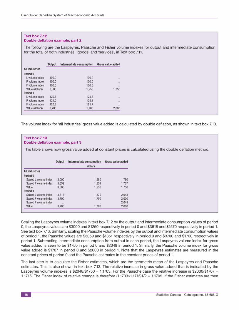
Text box 7.12 Double deflation example, part 2
The following are the Laspeyres, Paasche and Fisher volume indexes for output and intermediate consumption for the total of both industries, ‘goods’ and ‘services’, in Text box 7.11.
All industriesOutput Intermediate consumption Gross value added
Period 0L volume index 100.0 100.0 ...P volume index 100.0 100.0 ...F volume index 100.0 100.0 ...Value (dollars) 3,000 1,250 1,750
Period 1L volume index 120.6 125.6 ...P volume index 121.0 125.8 ...F volume index 120.8 125.7 ...Value (dollars) 3,700 1,700 2,000
The volume index for ‘all industries’ gross value added is calculated by double deflation, as shown in text box 7.13.
Text box 7.13 Double deflation example, part 3
This table shows how gross value added at constant prices is calculated using the double deflation method.
Output Intermediate consumption Gross value addeddollars
All industriesPeriod 0
Scaled L volume index 3,000 1,250 1,750Scaled P volume index 3,059 1,351 1,707Value 3,000 1,250 1,750
Period 1Scaled L volume index 3,618 1,570 2,048Scaled P volume index 3,700 1,700 2,000Scaled F volume index ... ... 2,049Value 3,700 1,700 2,000
Scaling the Laspeyres volume indexes in text box 7.12 by the output and intermediate consumption values of period 0, the Laspeyres values are $3000 and $1250 respectively in period 0 and $3618 and $1570 respectively in period 1. See text box 7.13. Similarly, scaling the Paasche volume indexes by the output and intermediate consumption values of period 1, the Paasche values are $3059 and $1351 respectively in period 0 and $3700 and $1700 respectively in period 1. Subtracting intermediate consumption from output in each period, the Laspeyres volume index for gross value added is seen to be $1750 in period 0 and $2048 in period 1. Similarly, the Paasche volume index for gross value added is $1707 in period 0 and $2000 in period 1. Note that the Laspeyres estimates are measured in the constant prices of period 0 and the Paasche estimates in the constant prices of period 1.
The last step is to calculate the Fisher estimates, which are the geometric mean of the Laspeyres and Paasche estimates. This is also shown in text box 7.13. The relative increase in gross value added that is indicated by the Laspeyres volume indexes is $2048/$1750 = 1.1703. For the Paasche case the relative increase is $2000/$1707 = 1.1715. The Fisher index of relative change is therefore (1.1703×1.1715)1/2 = 1.1709. If the Fisher estimates are then

Statistics Canada – Catalogue no. 13-606-G 17
User Guide: Canadian System of Macroeconomic Accounts
scaled to equal gross value added in the first of the two periods ($1750), the Fisher estimate of gross value added in period 1 is $1750×1.1709 = $2049.
In section 7.3.2 it is explained how the Laspeyres and Paasche volume indexes can be interpreted as expressing the transaction aggregates in the constant prices of the first or second periods respectively. Using this interpretation, the ‘double-deflation’ approach is effectively to restate the output and intermediate consumption transaction values in dollars of constant purchasing power, instead of in nominal dollars. Either the constant dollars of the first period (Laspeyres) or the constant dollars of the second period (Paasche) can be used. Then gross value added at constant prices is calculated by subtracting intermediate consumption at constant prices from output at constant prices. This yields two estimates of gross value added, one in the constant prices of the first period and the other in the constant prices of the second period. As a final step, these can be combined to produce Fisher estimates of gross value added in volume terms. This, in fact, is just what is done by Statistics Canada to produce the official estimates of gross value added in the supply and use accounts.
7.3.6 Consistency of Laspeyres, Paasche and Fisher price and volume indexes
Suppose a price or volume index A is the aggregate of two other indexes B and C and all three indexes are scaled to equal 100.0 in the initial period. Then A should lie somewhere between B and C. Moreover, if B has a greater weight than index C then A should be closer to B than C. This is an example of the property of consistency and it is a very desirable property for an index to have. The Laspeyres, Paasche and Fisher index number formulas all have this property. However, when two indexes of these kinds (two Laspeyres indexes, for example) are chained, they do not necessarily have this property for comparisons that cross the period where the indexes were chained (that is, the link period).
The problem of apparent inconsistency is illustrated in text box 7.14. It shows two Laspeyres price20 indexes, labelled P1 and P2. The first index extends from period 0 to period 2 and covers the prices of the three types of fruit. The second index covers the same types of fruit between periods 2 and 4. The two indexes have different weight structures. In addition, a third index is shown ranging from period 0 to period 4 which is the chained index, with period 2 as the link period.
In this example, the apparent inconsistency is evident in the fact that although the chained indexes for all three types of fruit individually show some degree of increase between period 0 and period 4, the aggregate index indicates a small decrease over this period.

Statistics Canada – Catalogue no. 13-606-G18
User Guide: Canadian System of Macroeconomic Accounts
Text box 7.14 Apparent inconsistency in chained indexes example
This table shows how apparent inconsistencies can sometimes arise when two indexes are chained and comparisons are made across the link period.
Apples Oranges Bananas Fruitindex
Laspeyres index P1Period 0 100.0 100.0 100.0 100.0Period 1 116.7 105.0 145.5 125.6Period 2 114.3 114.3 93.8 105.3Weights 1 0.24 0.32 0.44 1.00Laspeyres index P2Period 2 100.0 100.0 100.0 100.0Period 3 103.0 108.1 104.0 106.4Period 4 104.2 89.0 107.0 94.5Weights 2 0.30 0.65 0.05 1.00Chained Laspeyres indexPeriod 0 100.0 100.0 100.0 100.0Period 1 116.7 105.0 145.5 125.6Period 2 114.3 114.3 93.8 105.3Period 3 117.7 123.5 97.5 111.9Period 4 119.1 101.7 100.3 99.4
The chained index is apparently inconsistent because the value for total fruit declines between periods 0 and 4 while the values for each individual type of fruit increase over this time range.
Obvious inconsistencies such as this are uncommon, but they do arise from time to time in published time series. They are more likely to occur when the weight structures of the two indexes being chained are quite different, as in the example.
Apparent inconsistencies in chained indexes as illustrated in text box 7.14 can be a source of considerable concern and confusion for users of price and volume indexes unless this phenomenon is flagged and explained.
A related characteristic of the Laspeyres and Paasche formulas is that they are consistent in aggregation. This means, for example, that if one calculates a Laspeyres volume index based on the prices and quantities from one set of product transactions and one also calculates a second Laspeyres volume index based on the prices and quantities from another different set of product transactions, then the overall Laspeyres volume index representing both sets of transactions combined could be calculated either directly, from the individual prices and quantities in the combined data set, or indirectly by aggregating the two component Laspeyres indexes. Unfortunately the Fisher index is not consistent in aggregation, though it is approximately so.

Statistics Canada – Catalogue no. 13-606-G 19
User Guide: Canadian System of Macroeconomic Accounts
Text box 7.15 Base periods
When index numbers are discussed, the following base periods (sometimes called reference periods) come into play:
The time base period is the period, typically a year, in which the index is scaled to equal 100.0 (or some other value). When the index subsequently is rescaled so that it equals 100.0 (or some other value) in some other period, this is often called rebasing.
The weight base period is the period, typically a year, from which the index weights are drawn. In the case of a Laspeyres index, for example, this is the initial period. Sometimes this is simply called the weight period and changing the index from one weight base period to another is often called reweighting.
The price base period is the first of the two periods that are being compared by the index. The other period in the comparison is sometimes called the current period.
The link base period is the period in which one index is chained to another index.
It is possible for the time, weight, price (or current) and link periods to be the same, but they need not be so.
7.3.7 Elementary versus compound price and volume indexes
Suppose a sample of apple prices (average monthly) and quantities sold is collected in several stores within a given metropolitan area, once a month for a period of several months. A variety of different types of apples are sampled: large and small; fresh and not fresh; Cortland, McIntosh, Granny Smith, Red Delicious and so on. Then the Laspeyres, Paasche and Fisher index number formulas are used to construct apple price and volume indexes, making appropriate quality adjustments for the different types of apples. These are called elementary price and volume indexes because they are constructed from individual price and quantity data. Statistics Canada calculates many elementary price indexes every month as part of the compilation of the consumer price index and a variety of other price indexes.21
Now suppose a similar exercise is conducted for oranges and bananas, yielding elementary price and volume indexes for these fruits as well. How can the apple, orange and banana indexes be combined to produce price and volume indexes for fruit as a whole?
This calculation of compound price and volume indexes is done using the same Laspeyres, Paasche and Fisher index number formulas already described in equations (7.8) through (7.13). However, the 𝑝𝑝𝑖𝑖(𝑡𝑡) are taken to be the price indexes for the three fruit types, instead of the individual prices, and the 𝑞𝑞𝑖𝑖(𝑡𝑡) are obtained by deflating the aggregate transaction values of apples, oranges and bananas by their corresponding price indexes, rather than by using the individual quantities which are not commensurable. In addition, these compound index number calculations usually take advantage of a transformation of the Laspeyres and Paasche index number formulas.
The Laspeyres price index is transformed as follows:
(7.14)
𝑃𝑃𝐿𝐿 =∑𝑝𝑝𝑖𝑖(𝑡𝑡)𝑞𝑞𝑖𝑖(0)∑ 𝑝𝑝𝑖𝑖(0)𝑞𝑞𝑖𝑖(0)
=∑{𝑝𝑝𝑖𝑖(𝑡𝑡)/𝑝𝑝𝑖𝑖(0)}𝑝𝑝𝑖𝑖(0)𝑞𝑞𝑖𝑖(0)
∑𝑝𝑝𝑖𝑖(0)𝑞𝑞𝑖𝑖(0)
Equation (7.14) says that the Laspeyres price index can be calculated as a weighted average of the price relatives,𝑝𝑝𝑖𝑖(𝑡𝑡)/𝑝𝑝𝑖𝑖(0) , with the weights being the transaction value shares from the second of the two periods,
𝑝𝑝𝑖𝑖(0)𝑞𝑞𝑖𝑖(0)/∑𝑝𝑝𝑖𝑖(0)𝑞𝑞𝑖𝑖(0) . The advantage is that no quantity information, as such, is required in this version of the formula. Only transaction value shares are needed. A similar transformation can be applied to the Laspeyres volume index.

Statistics Canada – Catalogue no. 13-606-G20
User Guide: Canadian System of Macroeconomic Accounts
Similarly, the Paasche price index can be transformed as follows:
(7.15)
𝑃𝑃𝑃𝑃 =∑𝑝𝑝𝑖𝑖(𝑡𝑡)𝑞𝑞𝑖𝑖(𝑡𝑡)∑𝑝𝑝𝑖𝑖(0)𝑞𝑞𝑖𝑖(𝑡𝑡)
= [∑{𝑝𝑝𝑖𝑖(0)/𝑝𝑝𝑖𝑖(𝑡𝑡)}𝑝𝑝𝑖𝑖(𝑡𝑡)𝑞𝑞𝑖𝑖(𝑡𝑡)
∑ 𝑝𝑝𝑖𝑖(𝑡𝑡)𝑞𝑞𝑖𝑖(𝑡𝑡)]-1
Equation (7.15) says that the Paasche price index can be calculated as the inverse of a weighted average of the inverse of the price relatives 𝑝𝑝𝑖𝑖(0)/𝑝𝑝𝑖𝑖(𝑡𝑡) , with the weights being the transaction value shares from the second of
the two periods, 𝑝𝑝𝑖𝑖(𝑡𝑡)𝑞𝑞𝑖𝑖(𝑡𝑡)/∑𝑝𝑝𝑖𝑖(𝑡𝑡)𝑞𝑞𝑖𝑖(𝑡𝑡) .22 Again, no quantity information, as such, is required in this version of the formula. A similar transformation can be applied to the Paasche volume index.
The use of this transformation of the Laspeyres and Paasche price index formulas to create compound indexes is illustrated in text box 7.16.
Text box 7.16 Compound price indexes using the fruit example
Below are some hypothetical index numbers.
Apples Oranges Bananasindex
Period 0Price index 100.0 100.0 100.0Quantity index 100.0 100.0 100.0Value index 100.0 100.0 100.0Value share (ratio) 0.2400 0.3200 0.4400Period 1Price index 116.7 105.0 145.5Quantity index 150.0 200.0 80.0Value index 175.0 210.0 116.4Value share (ratio) 0.2618 0.4190 0.3192
The aggregate price indexes in period 1 for all types of fruit are calculated as follows:
Laspeyres P = 100 × (116.7 × 0.2400 + 105.0 × 0.3200 + 145.5 × 0.4400) = 125.6
Paasche P = 100 ÷ ((1/116.7) × 0.2618 + (1/105.0) × 0.4190 + (1/145.5) × 0.3192) = 118.6
Fisher P = 100 × (1.256 × 1.186)1/2 = 122.1
This formula for computing compound price indexes is essentially the one that Statistics Canada uses to calculate national accounts transaction aggregates from price and volume components. Thus, for example, consider the transaction aggregate ‘final household consumption expenditure on goods and services’. To calculate this aggregate, price indexes are first obtained for all the categories of spending making up total household consumption expenditure (food, clothing, etcetera). These price indexes are then divided into the values, at current prices, of the corresponding expenditures—this, again, is the process referred to as deflation. Finally, the price indexes together with the deflated expenditure values and the expenditure values themselves are used in the Laspeyres, Paasche and Fisher formulas to calculate the required price and volume indexes for total final household consumption expenditure on goods and services.

Statistics Canada – Catalogue no. 13-606-G 21
User Guide: Canadian System of Macroeconomic Accounts
In other words, while aggregate value series are built up by summing component value series, aggregate price and volume series are constructed by applying the index number formulas invented by Laspeyres, Paasche and Fisher to component price and volume indexes. As a practical matter, the aggregate indexes so obtained are generally more reliable the more detailed is the collection of lower-level price and volume indexes being aggregated.
7.3.8 Contributions to change
In the previous section a hypothetical example was considered in which fruit price indexes were calculated, using the Laspeyres, Paasche and Fisher index number formulas, by combining price index and transaction value information for three types of fruit: apples, oranges and bananas. In the example (text box 7.16) the Laspeyres price index for fruit increased 25.6% between the initial period and the second period. How can this percentage increase be broken down into three separate and additive contributions attributable to the three types of fruit? This is the contributions to change problem.
In the case of the Laspeyres index number formula, the calculation of such contributions to change is straightforward. It is illustrated for the Laspeyres price index in text box 7.17. The contribution of each type of fruit is equally dependent on the price increase for that type of fruit and on the transaction weight of that type of fruit in total expenditure. The calculations for the Laspeyres volume index are similar. Contributions to change for the Paasche index are rarely calculated and are not illustrated here.
Text box 7.17 Contributions to change in the Laspeyres price index using the fruit example
Text box 7.16 illustrates the calculation of a Laspeyres compound price index for fruit. The calculation is as follows:
Laspeyres P = (116.7 × 0.2400 + 105.0 × 0.3200 + 145.5 × 0.4400) = 125.6
This 25.6% increase in the price of fruit can be decomposed into three components as follows:
Apples: 16.7% × 0.24 = 4.0%
+ Oranges: 5.0% × 0.32 = 1.6%
+ Bananas: 45.5% × 0.44 = 20.0%
= Fruit: 25.6%

Statistics Canada – Catalogue no. 13-606-G22
User Guide: Canadian System of Macroeconomic Accounts
For the Fisher index number formula the calculation of contributions to change is not so simple. It turns out the contributions can be calculated using the approach shown in equation (7.16).
(7.16)
𝑃𝑃𝐹𝐹 − 1 = ∑ 𝑤𝑤𝑖𝑖 {𝑝𝑝𝑖𝑖(𝑡𝑡) − 𝑝𝑝𝑖𝑖(0)}
Where:
(7.17)
𝑤𝑤𝑖𝑖 = 𝑞𝑞𝑖𝑖(0)
∑ 𝑝𝑝𝑖𝑖(0)𝑞𝑞𝑖𝑖(0) + (𝑃𝑃𝐹𝐹)2 𝑞𝑞𝑖𝑖(𝑡𝑡)∑ 𝑝𝑝𝑖𝑖(𝑡𝑡)𝑞𝑞𝑖𝑖(𝑡𝑡)
1 + 𝑃𝑃𝐹𝐹
In this formula, 𝑃𝑃𝐹𝐹 is the Fisher price index comparing prices in period t to prices in period 0, 𝑝𝑝𝑖𝑖(0) is the price for component i in period 0, 𝑞𝑞𝑖𝑖(0) is the volume for component i in period 0, 𝑝𝑝𝑖𝑖(𝑡𝑡) is the price for component i in period t and 𝑞𝑞𝑖𝑖(𝑡𝑡) is the volume for component i in period t. The decomposition is illustrated in text box 7.18, using the fruit price data in text box 7.1.
The reason the formula is so complicated is that the Fisher index uses weights from two periods instead on just one, so the weights in the calculation of contribution to change must reflect relative price changes as well as relative quantity changes.
Statistics Canada – Catalogue no. 13-606-G 23
User Guide: Canadian System of Macroeconomic Accounts
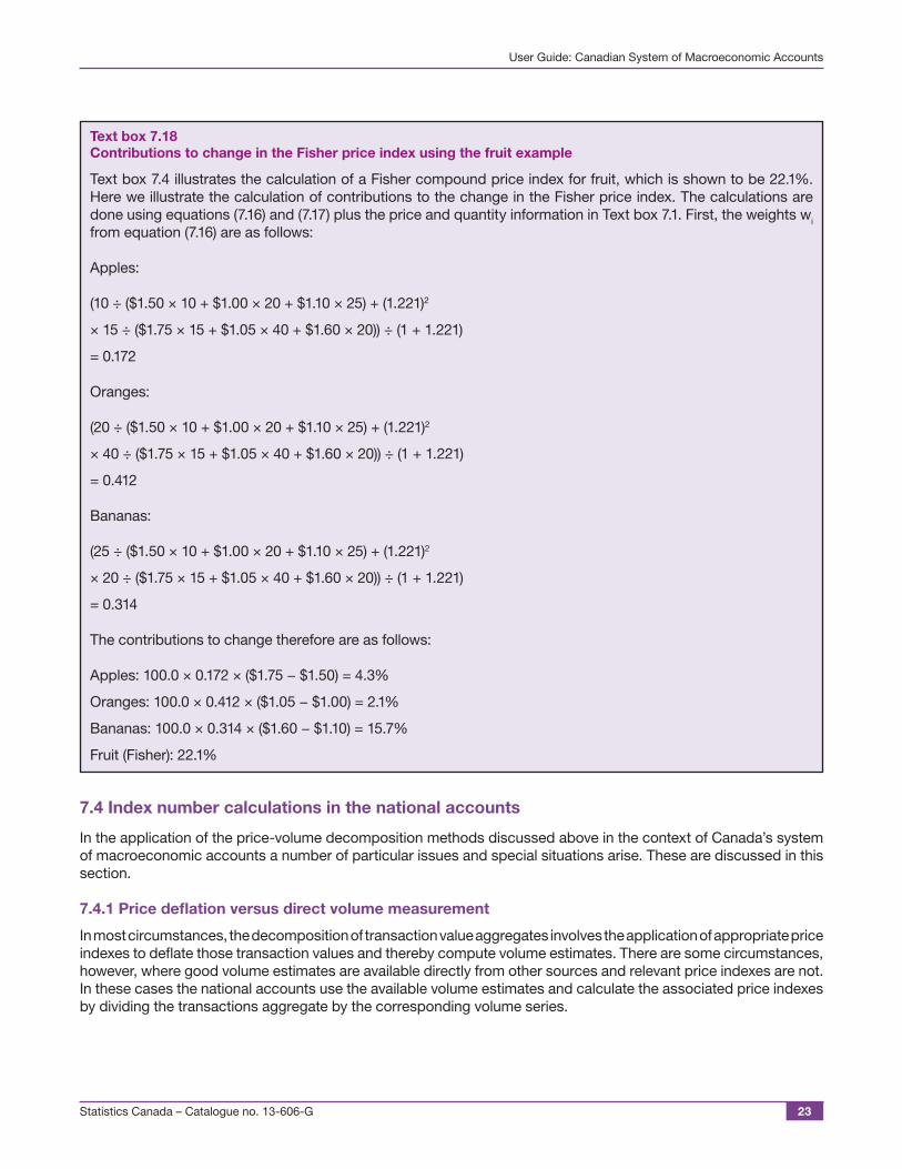
Text box 7.18 Contributions to change in the Fisher price index using the fruit example
Text box 7.4 illustrates the calculation of a Fisher compound price index for fruit, which is shown to be 22.1%. Here we illustrate the calculation of contributions to the change in the Fisher price index. The calculations are done using equations (7.16) and (7.17) plus the price and quantity information in Text box 7.1. First, the weights wi from equation (7.16) are as follows:
Apples:
(10 ÷ ($1.50 × 10 + $1.00 × 20 + $1.10 × 25) + (1.221)2
× 15 ÷ ($1.75 × 15 + $1.05 × 40 + $1.60 × 20)) ÷ (1 + 1.221)
= 0.172
Oranges:
(20 ÷ ($1.50 × 10 + $1.00 × 20 + $1.10 × 25) + (1.221)2
× 40 ÷ ($1.75 × 15 + $1.05 × 40 + $1.60 × 20)) ÷ (1 + 1.221)
= 0.412
Bananas:
(25 ÷ ($1.50 × 10 + $1.00 × 20 + $1.10 × 25) + (1.221)2
× 20 ÷ ($1.75 × 15 + $1.05 × 40 + $1.60 × 20)) ÷ (1 + 1.221)
= 0.314
The contributions to change therefore are as follows:
Apples: 100.0 × 0.172 × ($1.75 − $1.50) = 4.3%
Oranges: 100.0 × 0.412 × ($1.05 − $1.00) = 2.1%
Bananas: 100.0 × 0.314 × ($1.60 − $1.10) = 15.7%
Fruit (Fisher): 22.1%
7.4 Index number calculations in the national accounts
In the application of the price-volume decomposition methods discussed above in the context of Canada’s system of macroeconomic accounts a number of particular issues and special situations arise. These are discussed in this section.
7.4.1 Price deflation versus direct volume measurement
In most circumstances, the decomposition of transaction value aggregates involves the application of appropriate price indexes to deflate those transaction values and thereby compute volume estimates. There are some circumstances, however, where good volume estimates are available directly from other sources and relevant price indexes are not. In these cases the national accounts use the available volume estimates and calculate the associated price indexes by dividing the transactions aggregate by the corresponding volume series.

Statistics Canada – Catalogue no. 13-606-G24
User Guide: Canadian System of Macroeconomic Accounts
This approach is taken where the product classes involved are homogeneous. Examples include expenditures on electricity and natural gas. It is common for several product classes of merchandise exports and imports and for some components of final household consumption of goods and services. The volume estimates for a large part of government consumption expenditures are also calculated this way, since there are no market prices (or price indexes) associated with these series. The most important volume indicator for government consumption expenditures are hours worked by government employees. In rare instances no value measurements are directly available so these must be created by multiplying the price index by the volume index and scaling the resulting series to some benchmark value estimate.
7.4.2 Income and expenditure accounts deflation
The income and expenditure accounts are described in chapter 5. The GDP-by-expenditure table in those accounts is decomposed into price and volume components, both in the quarterly and annual national tables and in the annual provincial-territorial tables.23 Most of the volume estimates are calculated by deflating the final expenditure series by corresponding price indexes (chiefly from among those discussed in Annex A.7.1), although as noted in the previous section some are derived directly from volume indicators. The inventory change component is a special case that is discussed in section 7.5.2. Fixed-base quarterly Laspeyres volume indexes at constant prices from the year 2007 are available (36-10-0123-01) as well as quarterly chain-linked Fisher volume and price indexes (36-10-0104-01).
As already mentioned, aggregate indexes are generally more reliable the more detailed is the collection of lower-level price and volume indexes being aggregated. In the income and expenditure accounts, real GDP is made up from the level of detail described in Table 7.1. Many different price deflation approaches are used and the table highlights only the main ones.
Table 7.1Level of detail in the compilation of real GDP
Number of expenditure categories deflated Main deflator source1
Household final consumption expenditure 98 CPI
NPISH final consumption expenditure 1 SEPH
General governments final consumption expenditure 58 SEPH, LFS, CPI, IPPI
Residential structures investment expenditure 3 NHPI, MLS
Non-residential structures investment expenditure 2 NRBCPI, SEPH, IPPI
Machinery and equipment investment expenditure 9 MEPI
Intellectual property products investment expenditure 3 SEPH, LFS
NPISH investment expenditure 4 NRBCPI, SEPH, IPPI, MEPI
General governments investment expenditure 15 NRBCPI, SEPH, IPPI, MEPI
Investment in inventories 112 IPPI, CPI, WSPI
Exports of goods 90 IPPI, EIPI
Exports of services 4 IPPI, CPI
Imports of goods 90 BLS, EIPI
Imports of services 4 BLS
1. CPI = consumer price index, SEPH = survey of employment, payrolls and hours, LFS = labour force survey, IPPI = industrial product price index, NHPI = new housing price index, MLS = multiple listing service price index, NRBCPI = non-residential building construction price index, MEPI = machinery and equipment price index, WSPI = wholesale price index, EIPI = export-import price indexes, BLS = US Bureau of Labor Statistics price indexes.Source: Statistics Canada.

Statistics Canada – Catalogue no. 13-606-G 25
User Guide: Canadian System of Macroeconomic Accounts
7.4.3 Supply and use accounts deflation
The supply and use annual accounts are described in chapter 4. These accounts are also decomposed into price and volume components using the Laspeyres, Paasche and Fisher index number formulas. They are chained annually.
As is explained in chapter 4, the supply and use tables provide a very detailed description of the Canadian and provincial-territorial economies and their evolution through time. Most of the statistics in these tables have a product class dimension.24 Accordingly, price indexes (see Annex A.7.1) associated with the product classes can be used to deflate most of the supply and use tables.
The supply and use volume estimates thereby obtained are quite valuable from several perspectives. First, they reveal the trend in real outputs and inputs by industry and by product class. Second, the resulting estimates of GDP at basic prices that are calculated by double deflation (see section 7.3.5) provide annual benchmarks for the timelier monthly GDP by industry and annual provincial and territorial GDP by industry programs, as described in chapter 4. The estimates of supply and use at constant prices also serve as real input and output statistics for use in calculating multi-factor productivity by industry and province/territory. They are used as well in the environmental statistics program.
The supply and use tables at constant prices are produced around November each year with a lag of almost three years relative to the reference period. They can be obtained in Microsoft Excel files on request from Statistics Canada. The estimates are available separately for outputs, intermediate consumption and final demand categories.
The tables are deflated both at basic prices and at purchaser prices. This is accomplished by developing explicit deflators for the eight margin categories: wholesale, retail, taxes, gas, storage, natural gas pipeline transport, crude oil pipeline transport and other transport.
7.5 Deflation of stocks
The discussion so far has focussed on the price-volume decomposition as it applies to transaction flows. However, the non-financial asset stocks in the national balance sheet can also be decomposed into price and volume components. Accomplishing this gives rise to additional issues that are discussed in this section.
7.5.1 Fixed capital stocks
The balance sheets of institutional units such as corporations and governments typically report stocks of non-financial assets at historical cost25 minus depreciation. This means, for example, if a new corporation is formed in 2010 and invests (in machinery, equipment, plant and commercial real estate, say) $2 million that year, $1 million in 2011, $3 million in 2012 and $1.5 million in 2013, then its undepreciated non-financial assets at historical cost are $7.5 million. The corporation would normally depreciate these assets at rates permitted by the tax authorities,26 so its reported depreciated non-financial assets would be something less than $7.5 million.
The difficulties with these numbers from a national accounting perspective are that (i) they are measured in a mixture of prices from different accounting periods (for example, the $2 million investment in 2010 is measured in 2010 prices and the $1 million investment of 2011 is measured in 2011 prices) and (ii) the tax-based depreciation rates that have been applied are unlikely to line up with economic reality. What is needed, for national accounts purposes, is a valuation of cumulative investment at current prices27 with a deduction for the value of actual economic depreciation of that cumulative investment, also at current prices.

Statistics Canada – Catalogue no. 13-606-G26
User Guide: Canadian System of Macroeconomic Accounts
To address this kind of problem, non-financial asset values are normally constructed in a different manner, in preference to using the historical cost figures. The technique used is referred to as the perpetual inventory method (PIM). It is summarized in the following equation:
(7.18)
𝑆𝑆𝐾𝐾(𝑡𝑡) = 𝑆𝑆𝐾𝐾(𝑡𝑡 − 1) + 𝐼𝐼𝐾𝐾(𝑡𝑡) − 𝐷𝐷𝐾𝐾(𝑡𝑡) − 𝑂𝑂𝐾𝐾(𝑡𝑡)
Where S denotes a stock variable, I the corresponding investment variable, D the corresponding consumption of fixed capital variable and O the ‘other disappearance’ variable. The superscript ‘K’ is there to denote that all of these variables are Laspeyres volume measures. The equation simply states that the stock volume at the end of period t is equal to the stock volume at the end of the previous period t-1 plus any investment volume during the period t minus the consumption of fixed capital volume during period t minus any other disappearance of capital due, for example, to catastrophic weather loss.
According to SNA 2008, “consumption of fixed capital is the decline, during the course of the accounting period, in the current value of the stock of fixed assets owned and used by a producer as a result of physical deterioration, normal obsolescence or normal accidental damage.”28 This is sometimes referred to as economic depreciation. Occasionally the single word depreciation is also used as a synonym for consumption of fixed capital but the reader is cautioned that in normal business accounting the term most often refers to writing off historical capital costs at rates permitted by the tax authorities. In the national accounts the concept is one of economic depreciation—the decline in the value of an asset due to its physical deterioration, normal obsolescence or normal accidental damage—which is dependent on the current value of the asset, not its historical value.
Investment volumes are measured by deflating investment transaction flow statistics. The consumption of fixed capital variable is generally modelled29 by treating depreciation as a simple function ‘f’—such as a linear, geometric or hyperbolic function—of the stock at the end of the previous period, taking due account of the average life span (L) of the particular type of assets:
(7.19)
𝐷𝐷𝐾𝐾(𝑡𝑡) = 𝑓𝑓{𝑆𝑆𝐾𝐾(𝑡𝑡 − 1), 𝐿𝐿}
Given a starting value for the stock variable 𝑆𝑆𝐾𝐾(0) , an investment volume time series 𝐼𝐼𝐾𝐾(𝑡𝑡) , an estimate of the average life span of capital L and a choice for the functional form f, these two equations can be used to generate a stock volume time series 𝑆𝑆𝐾𝐾(𝑡𝑡) . Once this has been calculated, a corresponding capital stock series at current prices 𝑆𝑆𝐶𝐶(𝑡𝑡) can be obtained by multiplying the stock volume series by an appropriate investment price index. The resulting capital stock estimates are referred to as having been valued at replacement cost. In effect, the capital stock in the current period is valued at the current cost to replace that capital.
Table 7.2 illustrates this type of calculation. It shows stocks of fixed non-residential capital by asset type for the two years 2007 and 2008, both at current prices and at the constant prices of 2007. These statistics are calculated using a geometric depreciation function, with different average life-of-capital assumptions for each asset type. They are done using the Laspeyres index number formula, although chained Fisher estimates are also available.

Statistics Canada – Catalogue no. 13-606-G 27
User Guide: Canadian System of Macroeconomic Accounts
Table 7.2 Stocks of fixed non-residential capital by asset type
2007 2008 2009Current prices Current prices Constant 2007 prices
millions of dollars
Total non-residential 1,532,232 1,692,699 1,592,206Non-residential buildings 445,909 494,709 453,974Engineering construction 608,172 685,938 639,998Machinery and equipment 308,611 329,014 321,652
Textile products, clothing, and products of leather 466 421 416Wood products 229 235 224Plastic and rubber products 338 310 296Non-metallic mineral products 158 151 148Fabricated metallic products 3,303 3,334 3,220Industrial machinery 135,505 147,398 142,608Computer and electronic products 45,663 48,703 48,573Electrical equipment, appliances and components 13,943 14,827 13,971Transportation equipment 88,673 92,314 91,235Furniture and related products 17,386 18,336 18,011Other manufactured products and custom work 2,947 2,984 2,951
Intellectual property products 169,541 183,039 176,583Mineral exploration and evaluation 69,734 77,101 73,437Research and development 64,150 67,116 65,422Software 35,657 38,821 37,725
Source: Statistics Canada, table 36-10-0097-01.
7.5.2 Inventory stocks
A similar issue arises with respect to inventory stocks and flows. A business that acquires products for intermediate consumption or goods for resale records them in its inventories at cost. If they remain in inventory for more than one accounting period, inventories may be augmented in the following period at a different cost. When the goods are ultimately removed from inventory, either to be used in a production process or to be resold, a question arises as to what value should be attributed to them at removal, for accounting purposes.
Accountants suggest three alternative solutions to this problem, referred to as (i) first in, first out (FIFO), (ii) last in, first out (LIFO) and (iii) average cost valuation. Depending on which of these accounting conventions a business adopts, a firm’s recorded inventory stocks can have different interpretations.
Inventory stocks appear in the national balance sheet as a form of non-financial produced assets (see chapter 6). The period-to-period change in inventory stocks also appears in the GDP-by-expenditure table (see chapter 5).
To calculate inventory stocks and period-to-period inventory changes for national accounts purposes, the following steps are followed. First, estimates of inventory stocks are obtained from the balance sheets of businesses. These estimates are at historical cost, so it is not appropriate to deflate them with a current price index. Instead, a composite price index is calculated—a weighted average of current and lagged price indexes depending on the estimated average turnover period of inventories in the particular industry and the most common method of inventory accounting used by establishments in the industry. This deflation process yields an estimate of the inventory stock volume series. A corresponding inventory stock value series at current prices is calculated by multiplying the volume series by a current price index for the types of goods held in inventory. To calculate the value, at constant prices, of the physical change in inventories for purposes of the real GDP-by-expenditure table, the change in the inventory volume series is used. Finally, the value of the physical change in inventories at current prices is calculated by multiplying the corresponding change at constant prices by the current price index.
Statistics Canada – Catalogue no. 13-606-G28
User Guide: Canadian System of Macroeconomic Accounts
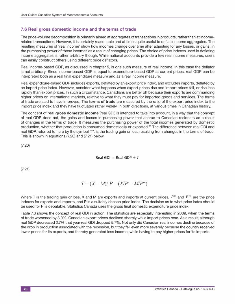
7.6 Real gross domestic income and the terms of trade
The price-volume decomposition is primarily aimed at aggregates of transactions in products, rather than at income-related transactions. However, it is certainly reasonable and at times quite useful to deflate income aggregates. The resulting measures of ‘real income’ show how incomes change over time after adjusting for any losses, or gains, in the purchasing power of those incomes as a result of changing prices. The choice of price indexes used in deflating income aggregates is rather arbitrary though. While national accounts provide a few real income measures, users can easily construct others using different price deflators.
Real income-based GDP, as discussed in chapter 5, is one such measure of real income. In this case the deflator is not arbitrary. Since income-based GDP is equal to expenditure-based GDP at current prices, real GDP can be interpreted both as a real final expenditure measure and as a real income measure.
Real expenditure-based GDP includes exports, deflated by an export price index, and excludes imports, deflated by an import price index. However, consider what happens when export prices rise and import prices fall, or rise less rapidly than export prices. In such a circumstance, Canadians are better off because their exports are commanding higher prices on international markets, relative to what they must pay for imported goods and services. The terms of trade are said to have improved. The terms of trade are measured by the ratio of the export price index to the import price index and they have fluctuated rather widely, in both directions, at various times in Canadian history.
The concept of real gross domestic income (real GDI) is intended to take into account, in a way that the concept of real GDP does not, the gains and losses in purchasing power that accrue to Canadian residents as a result of changes in the terms of trade. It measures the purchasing power of the total incomes generated by domestic production, whether that production is consumed domestically or exported.30 The difference between real GDI and real GDP, referred to here by the symbol ‘T’, is the trading gain or loss resulting from changes in the terms of trade. This is shown in equations (7.20) and (7.21) below.
(7.20)
Real GDI = Real GDP+ 𝑇𝑇
(7.21)
T = (X – M)/ P – (X/Px –M/Pm)
Where T is the trading gain or loss, X and M are exports and imports at current prices, 𝑃𝑃𝑥𝑥 and 𝑃𝑃𝑚𝑚 are the price indexes for exports and imports, and P is a suitably chosen price index. The decision as to what price index should be used for P is debatable. Statistics Canada uses the gross final domestic expenditure price index.
Table 7.3 shows the concept of real GDI in action. The statistics are especially interesting in 2009, when the terms of trade worsened by 3.0%. Canadian export prices declined sharply while import prices rose. As a result, although real GDP decreased 2.7% that year real GDI dropped 5.7%. Not only did Canadian real incomes decline because of the drop in production associated with the recession, but they fell even more severely because the country received lower prices for its exports, and thereby generated less income, while having to pay higher prices for its imports.
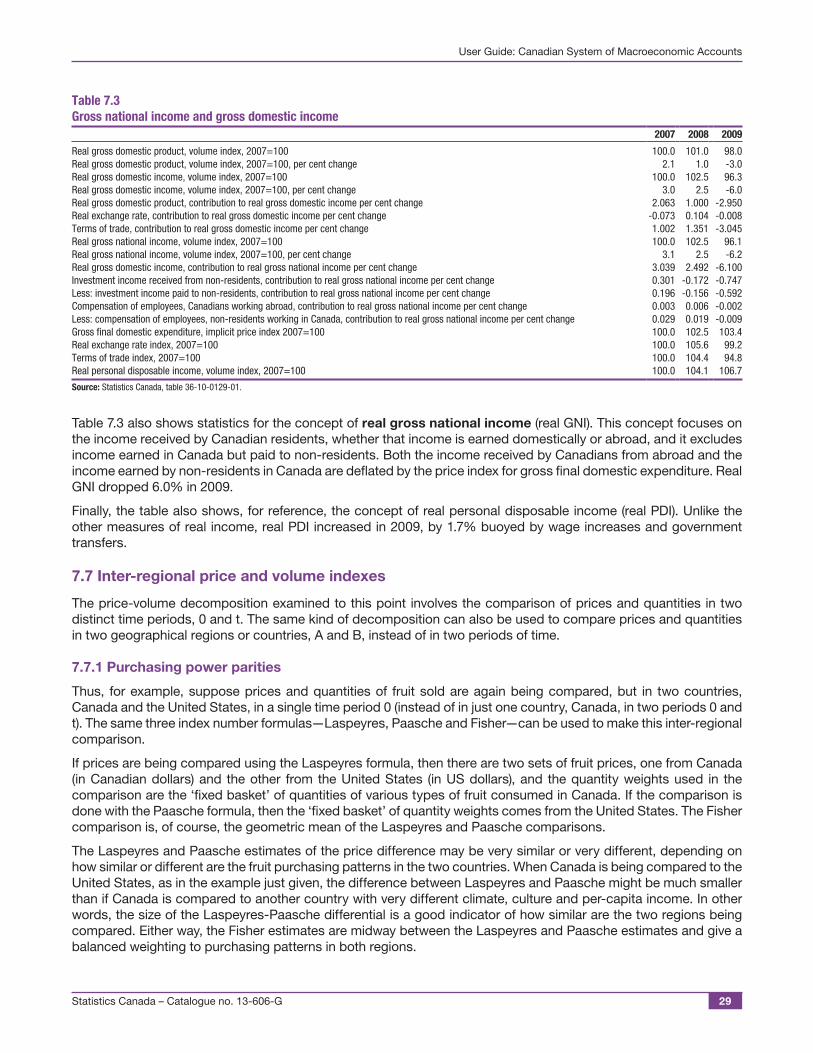
Statistics Canada – Catalogue no. 13-606-G 29
User Guide: Canadian System of Macroeconomic Accounts
Table 7.3 Gross national income and gross domestic income
2007 2008 2009
Real gross domestic product, volume index, 2007=100 100.0 101.0 98.0Real gross domestic product, volume index, 2007=100, per cent change 2.1 1.0 -3.0Real gross domestic income, volume index, 2007=100 100.0 102.5 96.3Real gross domestic income, volume index, 2007=100, per cent change 3.0 2.5 -6.0Real gross domestic product, contribution to real gross domestic income per cent change 2.063 1.000 -2.950Real exchange rate, contribution to real gross domestic income per cent change -0.073 0.104 -0.008Terms of trade, contribution to real gross domestic income per cent change 1.002 1.351 -3.045Real gross national income, volume index, 2007=100 100.0 102.5 96.1Real gross national income, volume index, 2007=100, per cent change 3.1 2.5 -6.2Real gross domestic income, contribution to real gross national income per cent change 3.039 2.492 -6.100Investment income received from non-residents, contribution to real gross national income per cent change 0.301 -0.172 -0.747Less: investment income paid to non-residents, contribution to real gross national income per cent change 0.196 -0.156 -0.592Compensation of employees, Canadians working abroad, contribution to real gross national income per cent change 0.003 0.006 -0.002Less: compensation of employees, non-residents working in Canada, contribution to real gross national income per cent change 0.029 0.019 -0.009Gross final domestic expenditure, implicit price index 2007=100 100.0 102.5 103.4Real exchange rate index, 2007=100 100.0 105.6 99.2Terms of trade index, 2007=100 100.0 104.4 94.8Real personal disposable income, volume index, 2007=100 100.0 104.1 106.7
Source: Statistics Canada, table 36-10-0129-01.
Table 7.3 also shows statistics for the concept of real gross national income (real GNI). This concept focuses on the income received by Canadian residents, whether that income is earned domestically or abroad, and it excludes income earned in Canada but paid to non-residents. Both the income received by Canadians from abroad and the income earned by non-residents in Canada are deflated by the price index for gross final domestic expenditure. Real GNI dropped 6.0% in 2009.
Finally, the table also shows, for reference, the concept of real personal disposable income (real PDI). Unlike the other measures of real income, real PDI increased in 2009, by 1.7% buoyed by wage increases and government transfers.
7.7 Inter-regional price and volume indexes
The price-volume decomposition examined to this point involves the comparison of prices and quantities in two distinct time periods, 0 and t. The same kind of decomposition can also be used to compare prices and quantities in two geographical regions or countries, A and B, instead of in two periods of time.
7.7.1 Purchasing power parities
Thus, for example, suppose prices and quantities of fruit sold are again being compared, but in two countries, Canada and the United States, in a single time period 0 (instead of in just one country, Canada, in two periods 0 and t). The same three index number formulas—Laspeyres, Paasche and Fisher—can be used to make this inter-regional comparison.
If prices are being compared using the Laspeyres formula, then there are two sets of fruit prices, one from Canada (in Canadian dollars) and the other from the United States (in US dollars), and the quantity weights used in the comparison are the ‘fixed basket’ of quantities of various types of fruit consumed in Canada. If the comparison is done with the Paasche formula, then the ‘fixed basket’ of quantity weights comes from the United States. The Fisher comparison is, of course, the geometric mean of the Laspeyres and Paasche comparisons.
The Laspeyres and Paasche estimates of the price difference may be very similar or very different, depending on how similar or different are the fruit purchasing patterns in the two countries. When Canada is being compared to the United States, as in the example just given, the difference between Laspeyres and Paasche might be much smaller than if Canada is compared to another country with very different climate, culture and per-capita income. In other words, the size of the Laspeyres-Paasche differential is a good indicator of how similar are the two regions being compared. Either way, the Fisher estimates are midway between the Laspeyres and Paasche estimates and give a balanced weighting to purchasing patterns in both regions.

Statistics Canada – Catalogue no. 13-606-G30
User Guide: Canadian System of Macroeconomic Accounts
A price index comparing prices in two regions or countries is often called a purchasing power parity (PPP). SNA 2008 defines the concept as follows: “Purchasing power parities (PPPs) are used in producing a reliable set of estimates of the levels of activity between countries, expressed in a common currency. A purchasing power parity (PPP) is defined as the number of units of B’s currency that are needed in B to purchase the same quantity of individual good or service as one unit of A’s currency purchase in A. Typically, a PPP for a country is expressed in terms of the currency of a base country, with the US dollar commonly being used. PPPs are thus weighted averages of the relative prices, quoted in national currency, of comparable items between countries. Used as deflators, they enable cross-country comparisons of GDP and its expenditure components.”31
In the fruit example, the Canadian prices are measured in Canadian dollars and the United States prices are measured in American dollars. If the currency exchange rate as gauged on international financial markets were one Canadian dollar to the American dollar, as it was in February 2013 for example, then one might expect the PPP to be near 1.0. In fact, however, currency exchange rates and purchasing power parities are often far apart. This is, to a degree, because purchasing power parities generally cover untraded products (notably real estate and untradeable services) as well as traded ones. Currency markets are much more focussed on tradable products—notably, in Canada’s case, oil and gas, other minerals, metals and agricultural products. The divergence between PPPs and currency exchange rates is also because currency exchange rates react, often sharply and rapidly, to shifting financial market attitudes and expectations whereas purchasing power parities reflect retail and wholesale prices that are determined by more fundamental longer-term supply and demand forces.
Table 7.4 shows purchasing power parity estimates for Canada and the United States. These statistics are estimates of the amount of United States currency required to buy the same quantity of a given class of products that one Canadian dollar purchases in Canada. They are based on benchmark estimates for the United States and Canada derived by the Organization for Economic Co-operation and Development (OECD) once every three years, from 1993 on.32 Interpolations between benchmark estimates are made using changes in the associated price indexes of the two countries. The estimates show, for example, that food, alcoholic beverages and tobacco, and clothing and footwear are substantially less expensive in the United States, in US dollars, than they are in Canada, in Canadian dollars, while health and education show the opposite relationship.

Statistics Canada – Catalogue no. 13-606-G 31
User Guide: Canadian System of Macroeconomic Accounts
Table 7.4 Canada-United States purchasing power parities
2007 2008 2009United States dollar per Canadian dollar
Gross domestic income (GDI) 0.860 0.861 0.847
Household final consumption expenditure 0.820 0.823 0.817Food and non-alcoholic beverages 0.690 0.716 0.681Alcoholic beverages and tobacco 0.512 0.499 0.543Clothing and footwear 0.629 0.630 0.686Housing, water, electricity, gas and other fuels 0.954 0.914 0.902Household furnishings, equipment and maintenance 0.705 0.727 0.728Health 1.042 1.038 1.020Transport 0.644 0.672 0.654Communication 0.878 0.936 0.952Recreation and culture 0.798 0.819 0.817Education 2.291 2.306 2.293Restaurants and hotels 0.669 0.694 0.697Miscellaneous goods and services 0.866 0.843 0.823Net purchases abroad 1.014 1.041 1.027
General governments final consumption expenditure 0.976 0.975 0.926Gross fixed capital formation 0.837 0.830 0.811
Construction 0.805 0.778 0.760Machinery and equipment 0.838 0.855 0.808
Changes in inventories 0.697 0.714 0.701Balance of exports and imports 0.859 0.861 0.847
Total goods 0.754 0.764 0.749Consumer goods 0.702 0.712 0.732
Durable goods 0.710 0.740 0.772Semi-durable goods 0.662 0.668 0.708Non-durable goods 0.695 0.718 0.673
Capital goods 0.832 0.829 0.795Total services 0.960 0.948 0.927
Consumer services 0.931 0.913 0.908Government services 0.976 0.975 0.926
Source: Statistics Canada, table 36-10-0365-01.
7.7.2 Real income comparisons across regions
Suppose you wanted to determine whether an average American household consumes more or less than a Canadian household. The problem is that the expenditures in the United States are in US dollars and the expenditures in Canada are in Canadian dollars. You could use the exchange rate to convert the Canadian expenditures into US dollars, but that might be misleading given exchange rates fluctuate widely from day to day and are often a poor indicator of price differentials. Instead you need either to express the Canadian expenditures at US prices or to express the US expenditures at Canadian prices. This means deflating the Canadian or US expenditures using purchasing power parities.
Table 7.5 shows indexes of real expenditures per capita in the United States relative to those in Canada for categories of gross domestic income (GDI). The term “real expenditure” is used here to express expenditure of the two countries in the same set of prices through the process of conversion with purchasing power parities (PPP). The use of the term “real” in a spatial context is analogous to its conventional use in time series, where expenditures made in different time periods are expressed in base period prices in order to measure their real growth. United States per capita expenditures in current dollars are converted to Canadian dollars by dividing them by the Fisher PPPs. These converted expenditures are then expressed as a ratio of Canadian expenditures per capita.

Statistics Canada – Catalogue no. 13-606-G32
User Guide: Canadian System of Macroeconomic Accounts
Table 7.5 Canada-United States comparison of real final expenditure per capita
2007 2008 2009U.S. expenditure relative to Canadian expenditure at PPP valuation
Gross domestic income (GDI) 116.9 113.0 118.8
Household final consumption expenditure 151.9 148.6 147.2Food and non-alcoholic beverages 133.4 128.6 127.0Alcoholic beverages and tobacco 135.0 139.8 135.3Clothing and footwear 158.3 155.2 139.4Housing, water, electricity, gas and other fuels 107.0 110.5 111.0Household furnishings, equipment and maintenance 136.3 125.0 122.6Health 571.3 567.2 575.1Transport 141.8 128.2 122.8Communication 138.3 133.4 123.4Recreation and culture 153.4 146.4 140.7Education 88.1 87.6 87.4Restaurants and hotels 167.2 160.4 158.4Miscellaneous goods and services 150.0 151.2 148.0Net purchases abroad -11.5 -15.7 -13.8
General governments final consumption expenditure 80.6 80.2 82.1Gross fixed capital formation 112.9 104.4 102.7
Construction 88.3 79.8 74.3Machinery and equipment 150.6 138.3 142.0
Changes in inventories 60.3 -48.8 419.2Balance of exports and imports -274.1 -322.4 221.0
Total goods 130.0 121.4 119.9Consumer goods 144.1 138.6 130.5
Durable goods 139.1 122.3 114.9Semi-durable goods 144.5 139.0 126.6Non-durable goods 151.0 146.3 150.5
Capital goods 112.1 100.8 100.6Total services 124.8 124.8 124.9
Consumer services 159.5 161.1 159.8Government services 80.6 80.2 82.1
Source: Statistics Canada, table 36-10-0365-01.
As can be seen in the table, US gross domestic income per capita is greater than Canadian gross domestic income per capita when the comparison is made using PPPs. Expenditures are over five times greater for health care and they are greater by varying amounts for most other expenditure categories in the table. However, per capita expenditures on education, construction and government services are lower in the US than in Canada. It should be readily understood why it is important to make these comparisons using actual household consumption rather than final household consumption expenditure (these concepts are discussed in chapter 5).
International institutions use PPPs in this way to compare the per capita incomes of all countries around the world and thereby identify priority areas for developmental assistance. The World Bank leads a multi-national effort every few years to estimate PPPs for all of its member countries which is known as the International Comparison Program.33
Annex A.7.1 Price indexes produced by Statistics Canada
Prices are the traffic control system of the market economy, serving to balance supply and demand for the wide range of products available. The relative movement of different prices provides valuable signals about which products are becoming more or less popular, where scarcities may be emerging, the impact of new trade restrictions or liberalization, the effects of technological change and innovation and various other economic developments.
Statistics Canada collects and publishes a lot of information about inter-temporal price changes, in the form of price indexes. These indexes are the principal ingredient in the national accounts price-volume decomposition calculation that is the focus of this chapter, along with the transaction aggregates, expressed at current prices, which are the targets for decomposition. The agency also releases a small number of spatial indexes, most notable the CPI intercity indexes and the Canadian remote post and foreign post price indexes.

Statistics Canada – Catalogue no. 13-606-G 33
User Guide: Canadian System of Macroeconomic Accounts
Annex A.7.1.1 Consumer price indexes
Consumer price indexes (CPIs)34 are the best known of the price indexes that Statistics Canada releases. Published monthly, they are closely followed by government and private sector organizations. Their coverage spans the full range of goods and services purchased by Canadian households and they line up quite well against the product classes of household final expenditure on consumer goods and services in the national accounts. This makes the CPIs an ideal source for use in the national accounts price-volume decomposition of this component of final demand. The CPIs measure market prices paid by consumers and include taxes and subsidies on products as well as transportation and distribution margins.
The CPI is calculated using the Lowe index number formula, which is a slightly more general version of the Laspeyres formula, discussed in section 7.3. In essence, the index can be thought of as a weighted average of price relatives for a set of product classes, where the weights are the shares of household expenditure on the different product classes and the price relatives are simply the ratios of the price of some product in the current period to the price of the same product in the previous period. The number of price relatives going into the calculation for each particular product class depends on the size of the statistical sample, which varies by product class. The CPI weights are derived primarily from the Survey of Household Spending and the sample of prices is collected mostly by Statistics Canada staff who visit retail stores each month and observe listed prices.
Text box A.7.1.1 Price relatives
A price relative is simply one price divided by another price. Most often the numerator is the current price of some product or class of products and the denominator is the price of that same product or class of products in the previous time period. Some other examples of price relatives are the current price divided by the price one year ago, the current price divided by some higher-level aggregate price (such as the all-items CPI) or the current price in one country divided by the current price of the same product in another country.
There are numerous complications and special cases in the CPI methodology, not least among which are the difficult challenges involved in adjusting for quality changes in certain types of products. Canada’s CPI structure and methodology are explained in considerable detail in The Canadian Consumer Price Index Reference Paper, Statistics Canada catalogue #62-553-X, released December 18, 2015.
Annex A.7.1.2 Industrial product price indexes
The industrial product price indexes (IPPIs)35 differ from the CPIs primarily in terms of their scope. They measure price changes for goods sold by manufacturers in Canada, usually to other producers rather than to households. Also included are non-residential electric power selling prices and raw materials’ prices. The sample of prices collected is for goods sold at basic prices.36 Accordingly, the prices covered by the IPPIs refer not to what a purchaser pays, but to what a producer receives. They exclude all taxes on products, such as sales taxes, since this money does not go to producers. They also exclude transportation services provided by common carriers beyond the factory gate and any distribution services performed by the retail or wholesale trade industries.
The IPPIs measure price changes by product class, based on the North American Product Classification System, as well as by industry, based on the North American Industry Classification System. They cover a wide range of products that may be part of the intermediate consumption of some businesses, or purchased for resale by wholesalers and retailers, or exported. These price indexes are used extensively in the price-volume decomposition for output, intermediate consumption and final demand in the supply and use accounts. They are also used extensively in the calculation of monthly real GDP by industry for Canada and annual real GDP by industry for provinces and territories. Finally, the IPPIs are also used in the deflation of the income and expenditure accounts, especially with regard to the components of fixed capital formation, inventory change and merchandise exports.

Statistics Canada – Catalogue no. 13-606-G34
User Guide: Canadian System of Macroeconomic Accounts
Like the CPI, the IPPI is calculated using the Lowe index number formula. The index weights are taken from the Annual Survey of Manufactures and Logging. The sample of monthly price quotes is collected from business establishments mostly by means of mail-out questionnaires. Efforts are made to collect transaction prices, including any typical discounts, rather than list prices.
Annex A.7.1.3 Machinery and equipment price indexes
The machinery and equipment price indexes (MEPIs) provide estimates of price change for machinery and equipment purchased by industries in Canada. The indexes are released both by product class and by industry of purchase and they are available quarterly.37
While the IPPIs focus on the suppliers of Canadian manufactured goods, the MEPIs are concerned with the demand side and are limited to machinery and equipment products. Their target population consists of all industries that purchase machinery and equipment, whether domestically produced or imported. Ideally the MEPIs would measure purchasers’ prices including taxes, tariffs, transportation costs and other margins, but because of the data sources used they are in fact measured mostly at basic prices.
There is no specific survey associated with the MEPIs. Rather, the price indexes are derived using data from other sources, notably the industry producer price index survey, the computer and peripherals price index survey and the United States Bureau of Labor Statistics producer price and export price indexes. The weights for the price indexes are derived from the final demand table of the supply and use accounts.
The MEPIs are used in the supply and use accounts and the income and expenditure accounts to deflate machinery and equipment capital expenditures and certain components of merchandise imports.
Annex A.7.1.4 Agriculture price indexes
The agriculture price indexes consist of the monthly farm product price indexes (FPPIs) and the quarterly farm input price indexes (FIPIs).38 The former measures the changes in prices that farmers receive for the agriculture products they produce and sell whereas the latter estimates the change in prices that farmers pay for inputs into their farming operations.
In the case of the FPPIs, the prices of products sampled are basic prices. The price index has separate crop and livestock components and is available by province as well as for Canada as a whole. The target population includes all Canadian agricultural operations as defined by the Census of Agriculture as well as marketing boards and agencies. Samples are selected and weighted using data from the farm cash receipts survey.
In the case of the FIPIs, the prices measured are for the full range of farm inputs including buildings, machinery and motor vehicles, fuel, repairs, seed, fertilizers, pesticides, insurance, stabilization premiums, wages, livestock purchases, feed, veterinary fees and drugs and some other costs. The goal is to measure purchaser prices. There is no specific survey for the FIPIs. Rather, the price indexes are constructed using price data from other sources such as the IPPIs, the MEPIs, the FPPIs, the CPIs, the labour force survey and some administrative data sources.
Annex A.7.1.5 Construction price indexes
The construction price indexes provide measures of the average change in prices of various types of building and other construction. These price indexes are among the most challenging to construct because construction projects tend to be large, expensive and quite heterogeneous. The fact that the price of the land on which the construction takes place is often included in the purchase price also complicates matters. There are three construction-related price indexes, focused on housing, apartment buildings and non-residential buildings.39
The new housing price index (NHPI) is a monthly series that measures changes over time in contractors’ selling prices of new residential houses (single, semi-detached and row), where detailed specifications pertaining to each house remain the same between two consecutive periods. The index is available for provinces but not territories, and for 21 metropolitan areas. Indexes are available for the total price, the land component and the residual component.
Statistics Canada – Catalogue no. 13-606-G 35
User Guide: Canadian System of Macroeconomic Accounts
The apartment building construction price index (ABCPI) is a quarterly series measuring changes in contractors’ selling prices of a representative apartment building. The non-residential building construction price index (NRBCPI) is a quarterly series measuring the changes in contractors’ selling prices of non-residential building construction (offices, warehouses, shopping centres, light factories, schools). Both of these indexes exclude the cost of land, land assembly, design, development and real estate fees. They collect price quotes in seven large census metropolitan areas.
The construction price indexes are used in the national accounts to deflate residential and non-residential capital formation estimates and to calculate estimates of the capital stock and the rates of capacity utilization.
Annex A.7.1.6 Services producer price indexes
The services producer price indexes (SPPIs) are relatively new indexes, so the length of the time series is typically shorter than is the case for the goods and construction price indexes. They aim to measure changes in the selling prices of products from a range of different business-services-producing industries including:
• traveller accommodation services;
• accounting services;
• couriers and messengers services;
• informatics professional services;
• passenger air services;
• retail services;
• wholesale services;
• commercial and industrial machinery and equipment rental and leasing services;
• commercial rental services;
• new lending services;
• for-hire motor carrier freight services; and
• architectural, engineering and related services.
They are intended as a complement to the industrial product price indexes, which are focused on goods.40
Measuring price change for business services is generally more challenging than for goods because the products sold are often differentiated (specialized to the customer) and also because their nature tends to change over time. It can be difficult to collect representative price quotes comparing identical products in two different time periods. Sometimes it is necessary to measure product price change indirectly by measuring changes in input costs instead. Each service category has a methodology that is uniquely tailored to its particular circumstances.
The SPPIs are used primarily in the supply and use accounts for deflating outputs and intermediate inputs by industry.
Annex A.7.1.7 International merchandise trade price indexes
Statistics Canada also produces export and import price indexes, by product class. These indexes are derived from a wide range of diverse data sources.
Some of these price indexes are calculated directly from the Customs trade data. Those data, which are reported by exporters and importers when their goods cross the border, provide physical quantity as well as value information, which allows price changes to be inferred by means of unit values. However, this approach works well only for certain homogeneous products.
For homogeneous products that do not flow through Customs channels, price data are available from other specific sources. In the case of cross-border trade in electricity, price information is available from the National Energy Board. For exports of crude petroleum and natural gas, price data come from Statistics Canada’s surveys of the energy sector.

Statistics Canada – Catalogue no. 13-606-G36
User Guide: Canadian System of Macroeconomic Accounts
In the case of exports, IPPIs and FPPIs are used for many manufactured and some agricultural products. For imports, producer price indexes from the United States Bureau of Labor Statistics are used for a large portion of imported manufactured products, since the majority of Canada’s merchandise imports come from the United States. The corporate goods price index’s export component, published by the Bank of Japan, is used as an indicator of price change for goods imported from Asia.
For a small number of selected representative products, Statistics Canada also collects export and import price data directly from Canadian exporters and importers, using a questionnaire with telephone follow-up.
The export and import price indexes are calculated in two sets, one based on the Laspeyres formula and the other the Paasche formula.41 These price indexes are used both in the supply and use accounts and in the income and expenditure accounts to calculate the volume of trade as well as chained Fisher price and volume indexes of gross domestic product at market prices. The trade price indexes are also useful for purposes of analyzing the terms of trade and the impact of changes in these terms on Canadian incomes.

Statistics Canada – Catalogue no. 13-606-G 37
User Guide: Canadian System of Macroeconomic Accounts
Notes for chapter 7
1. One often sees the term ‘quantity’ used in textbooks on index numbers, instead of the term ‘volume’. National accountants generally prefer the latter term because the former term, taken literally, can be misleading when the quality of products varies. Volume changes should be interpreted as comprising changes in both quantity and quality. Price changes should be seen as ‘pure’ price changes, comprising changes in prices that have been adjusted to remove the effects of quality change. For more on this point see section 7.3.
2. Two things are commensurable if they are measurable or comparable by a common standard.
3. Another scale that is convenient in some circumstances is to set the index equal to 1.0 in some arbitrary period.
4. International Labour Office, International Monetary Fund, Organization for Economic Co-operation and Development, Statistical Office of the European Communities (Eurostat), United Nations and the World Bank, Consumer Price Index Manual: Theory and Practice, Geneva, 2004 and Producer Price Index Manual: Theory and Practice, Geneva, 2004 (both available free on the Internet).
5. Bloem, Adriaan, J. Dippelsman and N. Maehle, Quarterly National Accounts Manual: Concepts, Data Sources and Compilation, International Monetary Fund, Washington D.C., 2001, chapter IX. (Available free on the Internet.)
6. Other examples would be when the amount of product in the package changes, or when the associated product warranty changes, or certain services that were formally included with a good are no longer provided, or in the case of a service product when the effectiveness of the service noticeably improves.
7. A variety of methods have been devised for adjusting an observed price change to remove the effects of quality change. If the quality difference is solely due to a change in the quantity of product in the package, for example, a pro rata adjustment can be made. For changes to more complex products, such as high-tech equipment, the hedonic modelling method is sometimes used although this approach is increasingly seen as overly expensive and not totally effective. A much simpler alternative is group mean imputation.
8. Readers wishing to look at the original references attributed to these three statisticians, or to other index number statisticians mentioned in this chapter, are referred to the extensive bibliographies in the two international manuals cited in the previous section.
9. The reader should note again that, as in equation (7.7), the symbols P, Q and V represent price, volume and value indexes of relative aggregate change. That is, for example, P represents the relative aggregate change in prices between two periods, 0 and t, not the average level of prices as in equation (7.4).
10. The Laspeyres price index as described represents an aggregation of individual prices, weighted by quantities from the initial period 0. However, it should be noted that (higher-level) price and volume indexes can also represent aggregations of (lower-level) price and volume indexes rather than individual prices. See section 7.3.7.
11. A similar but slightly more general version of the Laspeyres price index is the Lowe price index, first proposed by Joseph Lowe in 1823, wherein the quantity weights need not necessarily come from the index’s initial period 0, but can rather come from any period. Most price indexes released by Statistics Canada, such as the consumer price index and the industrial product price index, are derived using the Lowe formula.
12. Most of the monthly price indexes released by Statistics Canada such as the consumer price index and the industrial product price index use a variant of the Laspeyres formula rather than the Paasche formula. The principle reason is that source data for the quantity weights are usually available only with a substantial lag, which makes the Paasche formula impractical.
13. Alternatively, the arithmetic average can be used instead of the geometric average as proposed by Drobisch, Sidgwick and Bowley. However, the statistical properties of this alternative approach are such that the geometric average is universally the preferred method. For non-negative relatives the natural average is the geometric average.
14. The OECD online Glossary of Statistical Terms defines superlative indexes as “price or quantity indexes that are ‘exact’ for a flexible aggregator. A flexible aggregator is a second-order approximation to an arbitrary production, cost, utility or distance function. Exactness implies that a particular index number can be directly derived from a specific flexible aggregator.” Again, for bibliographical references see the two international manuals referred to

Statistics Canada – Catalogue no. 13-606-G38
User Guide: Canadian System of Macroeconomic Accounts
earlier in this chapter. Two other ‘superlative’ index number formulas are credited to Törnqvist and Theil, and to Walsh.
15. In the professional literature, an index number formula with this property is said to pass the factor reversal test.
16. In a practical application of the two index number formulas, the Paasche index could also be greater than the Laspeyres index because the population of buyers changes between the two periods, or because the preferences of the original buyers for one product as compared to another might change. Nevertheless, the empirical evidence indicates quite strongly that Laspeyres indexes tend to increase more rapidly than Paasche indexes.
17. A similar point can be made about a Paasche index with fixed weights from the current period being used for past periods—the current period weights are likely to become increasing unrepresentative as one moves to earlier periods.
18. In the professional literature, an index number formula with this property is said to pass the time reversal test.
19. Quarterly chained Fisher estimates are not calculated with the unadjusted data because they would suffer from the same seasonal drift problem alluded to earlier.
20. The indexes could just as well be Laspeyres volume indexes. The same conclusions could be drawn.
21. For most of the price indexes produced by Statistics Canada, such as the CPI and the IPPI, individual price observations cannot be weighted by quantities, in the calculation of elementary price indexes, for the simple reason that no quantity information is available at this low level (although this may change in future if it becomes feasible to use scanner data from retailers). Instead, the individual price observations are typically expressed as period-to-period price relatives and the unweighted geometric mean is then calculated. In the national accounts, indexes are typically calculated at a somewhat higher level where quantity and price information are both available.
22. In other words, the Paasche price index is the weighted harmonic mean of the price relatives.
23. The quarterly volume and price estimates are available in tables 36-10-0104-01, 36-10-0106-01 and 36-10-0123-01. The annual national estimates are in table 36-10-0369-01 and the associated annual contributions to percentage change estimates are in tables 36-10-0128-01, 36-10-0131-01, 36-10-0132-01, 36-10-0133-01 and 36-10-0135-01 The annual provincial and territorial estimates are in table 36-10-0222-01.
24. The exception is the primary income tables, for which no price indexes are available.
25. Also referred to as ‘book values’.
26. Canada’s tax laws permit corporations to depreciate, in their corporate accounts, their capital investments at rates which are accelerated relative to the true or economic rates of depreciation of those assets.
27. In the context of economic accounting, the term current is used to refer to the time at which the economic activity took place. ‘Current period’ means the period of observation. It does not mean the present time nor the time of compilation. Values are said to be expressed in ‘current prices’ if the prices used in the valuation of goods and services are those prevailing in the period of observation, that is both the quantity and the price components of the value series relate to the current period.
28. See SNA 2008, page 123.
29. Unfortunately there are no transaction flows associated with consumption of fixed capital. Rather, the depreciation process goes on rather quietly behind the scenes, one might say, and is unobserved. It is modelled in the national accounts and this lends an element of arbitrariness to all the variables with which consumption of fixed capital is associated. This is perhaps the main reason why net domestic product tends to receive less attention than gross domestic product.
30. Real gross domestic income is a concept that is defined in real terms only. There is no corresponding nominal measure.
31. See SNA 2008, page 318.
32. The OECD’s purchasing power parity estimates are available free on the Internet at oecd.org.

Statistics Canada – Catalogue no. 13-606-G 39
User Guide: Canadian System of Macroeconomic Accounts
33. For more information via the Internet see worldbank.org.
34. The consumer price indexes are in tables 18-10-0004-01 to 18-10-0006-01. The index weights are in 18-10-0007-01.
35. The industrial product price indexes for manufacturing goods and industries are available in tables 18-10-0029-01 to 18-10-0032-01. The electric power selling price indexes are in 18-10-0028-01 and the raw materials price indexes are in 18-10-0034-01.
36. ‘Basic prices’ are discussed in chapter 4.
37. The machinery and equipment price indexes are available in tables 18-10-0057-01 and 18-10-0058-01.
38. The farm product price indexes and the farm input price indexes are available in tables 32-10-0098-01 and 18-10-0023-01 respectively.
39. The three indexes are available in tables 18-10-0052-01 and 18-10-0050-01.
40. These indexes are available in tables 18-10-0020-01, 18-10-0021-01, 18-10-0024-01 to 18-10-0027-01, 18-10-0033-01, 18-10-0035-01 to 18-10-0037-01, 18-10-0040-01, 18-10-0041-01, 18-10-0043-01, 18-10-0045-01 and 18-10-0072-01.
41. These formulas are explained in section 7.3.


