User’s Guide for Biome-BGCMuSo 6.0 by Dóra HIDY 1 , Zoltán BARCZA 2,3,4 , Roland HOLLÓS 1 , Peter E. THORNTON 5 , Steven W. RUNNING 6 and Nándor FODOR 7 1 Excellence Center, Faculty of Science, Eötvös Loránd University, H-2462 Martonvásár, Brunszvik u. 2., Hungary 2 Department of Meteorology, Eötvös Loránd University, H-1117 Budapest, Pázmány P. s. 1/A, Hungary. 3 Excellence Center, Faculty of Science, Eötvös Loránd University, H-2462 Martonvásár, Brunszvik u. 2., Hungary 4 Czech University of Life Sciences Prague, Faculty of Forestry and Wood Sciences, Kamýcká 129, 165 21 Prague 6, Czech Republic 5 Climate Change Science Institute and Environmental Sciences Division, Oak Ridge National Laboratory, Oak Ridge, TN 37831, USA. 6 Numerical Terradynamic Simulation Group, Department of Ecosystem and Conservation Sciences, University of Montana, Missoula, MT 59812, USA. 7 Centre for Agricultural Research, Hungarian Academy of Sciences, H-2462 Martonvásár, Brunszvik u. 2., Hungary [November, 2019]
Transcript
User’s Guide for Biome-BGCMuSo 6.0
by Dóra HIDY1, Zoltán BARCZA2,3,4, Roland HOLLÓS1, Peter E. THORNTON5, Steven W. RUNNING6 and Nándor FODOR7
1 Excellence Center, Faculty of Science, Eötvös Loránd University, H-2462 Martonvásár, Brunszvik u. 2.,
Hungary 2 Department of Meteorology, Eötvös Loránd University, H-1117 Budapest, Pázmány P. s. 1/A, Hungary.
3 Excellence Center, Faculty of Science, Eötvös Loránd University, H-2462 Martonvásár, Brunszvik u. 2.,
Hungary 4 Czech University of Life Sciences Prague, Faculty of Forestry and Wood Sciences, Kamýcká 129, 165 21
Prague 6, Czech Republic 5 Climate Change Science Institute and Environmental Sciences Division, Oak Ridge National Laboratory, Oak
Ridge, TN 37831, USA. 6
Numerical Terradynamic Simulation Group, Department of Ecosystem and Conservation Sciences, University
of Montana, Missoula, MT 59812, USA. 7 Centre for Agricultural Research, Hungarian Academy of Sciences, H-2462 Martonvásár, Brunszvik u. 2.,
One major difference between the earlier versions of Biome-BGC and BBGCMuSo is
that in BBGCMuSo standing dead biomass and cut-down biomass pools are also defined.
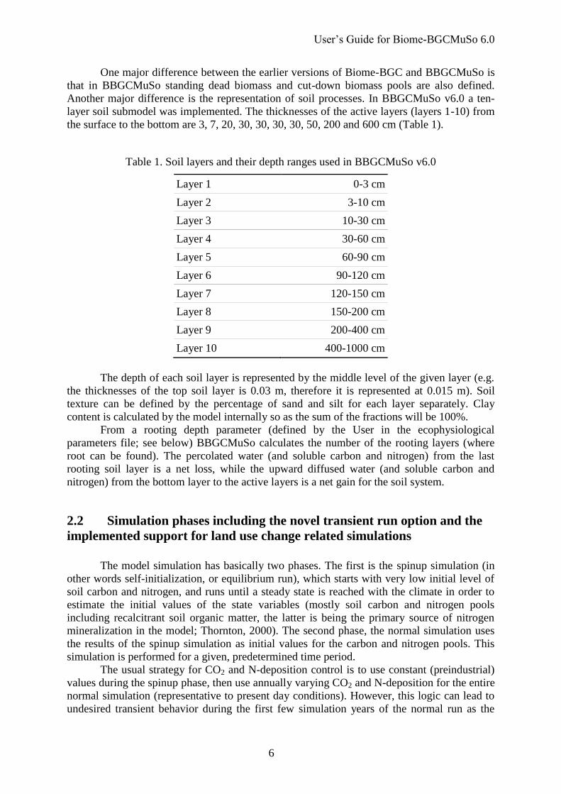
Another major difference is the representation of soil processes. In BBGCMuSo v6.0 a ten-
layer soil submodel was implemented. The thicknesses of the active layers (layers 1-10) from
the surface to the bottom are 3, 7, 20, 30, 30, 30, 30, 50, 200 and 600 cm (Table 1).
Table 1. Soil layers and their depth ranges used in BBGCMuSo v6.0
Layer 1 0-3 cm
Layer 2 3-10 cm
Layer 3 10-30 cm
Layer 4 30-60 cm
Layer 5 60-90 cm
Layer 6 90-120 cm
Layer 7 120-150 cm
Layer 8 150-200 cm
Layer 9 200-400 cm
Layer 10 400-1000 cm
The depth of each soil layer is represented by the middle level of the given layer (e.g.
the thicknesses of the top soil layer is 0.03 m, therefore it is represented at 0.015 m). Soil
texture can be defined by the percentage of sand and silt for each layer separately. Clay
content is calculated by the model internally so as the sum of the fractions will be 100%.
From a rooting depth parameter (defined by the User in the ecophysiological
parameters file; see below) BBGCMuSo calculates the number of the rooting layers (where
root can be found). The percolated water (and soluble carbon and nitrogen) from the last
rooting soil layer is a net loss, while the upward diffused water (and soluble carbon and
nitrogen) from the bottom layer to the active layers is a net gain for the soil system.
2.2 Simulation phases including the novel transient run option and the
implemented support for land use change related simulations
The model simulation has basically two phases. The first is the spinup simulation (in
other words self-initialization, or equilibrium run), which starts with very low initial level of
soil carbon and nitrogen, and runs until a steady state is reached with the climate in order to
estimate the initial values of the state variables (mostly soil carbon and nitrogen pools
including recalcitrant soil organic matter, the latter is being the primary source of nitrogen
mineralization in the model; Thornton, 2000). The second phase, the normal simulation uses
the results of the spinup simulation as initial values for the carbon and nitrogen pools. This
simulation is performed for a given, predetermined time period.
The usual strategy for CO2 and N-deposition control is to use constant (preindustrial)
values during the spinup phase, then use annually varying CO2 and N-deposition for the entire
normal simulation (representative to present day conditions). However, this logic can lead to
undesired transient behavior during the first few simulation years of the normal run as the
User’s Guide for Biome-BGCMuSo 6.0
7
user may introduce a sharp change for the CO2 and/or N-dep data (both are important drivers
of plant growth).
In order to avoid this undesired sharp change in the environmental conditions between
spinup and normal phase, a third simulation phase, a so-called transient simulation was
implemented in BBGCMuSo. According to the modifications, now it is possible to make an
automatic transient simulation after the spinup phase simply using the spinup INI file settings
(and some ancillary files; see later). In other words, now it is possible to initiate 3 consecutive
simulations instead of the usual two phases (triggered by the spinup and normal INI file).
As management might play an important role in site history and consequently in the
biogeochemical cycles, in BBGCMuSo the new transient simulation can include management,
in an annually varying fashion. The settings of management optionally defined within the
initialization file of the spinup are only used during the transient run, but not during the
regular spinup phase.
Another new feature was added to BBGCMuSo v6.0 that is also related with the
proper simulation of site history. As the spinup phase is usually associated with preindustrial
conditions, the normal phase might represent a plant functional type that is different from the
one present in the spinup phase. For example, present-day croplands occupy land that was
originally forest or grassland, so in this case spinup will simulate forest in equilibrium, and
the normal phase will simulate croplands. Another example is the simulation of afforestation
that might require spinup for grasslands, and normal phase for woody vegetation. We may
refer to these scenarios as land use change (LUC) related simulations. One problem that is
associated with LUC is the frequent crash of the model with the error 'negative nitrogen pool'
during the beginning of the normal phase. This error is typical if the spinup and normal EPC
files differ in terms of plant C:N ratios. The explanation of the error is not simple (and
elimination of the error is indeed a hard task) due to the model logic: in BBGC changes
within the defined pools due to e.g. allocation, litterfall, litter and soil organic matter
decomposition etc. are calculated at the end of each simulation day. Due to this day-end
calculations inconsistency might arise between available mineralized N and N demand by the
plant, and this might cause negative nitrogen pool.
In order to avoid this error, we have implemented an automatism that solves this problem.
According to the changes only the equilibrium carbon pools are passed to the normal phase
from the endpoint (restart) file. The endpoint nitrogen pools are calculated by the model code
so that the resulting carbon to nitrogen ratios are harmonized with the C:N ratio of the
different plant compartments presented in the EPC file of the normal phase. This modification
means that equilibrium nitrogen pools are not passed to the normal phase at all, but in our
interpretation this issue is compensated with the fact that LUC and site history can be
simulated properly.
User’s Guide for Biome-BGCMuSo 6.0
8
3. Input files
3.1 Overview
BBGCMuSo uses at least four input files each time it is executed. A brief description
of all files is given first, followed by detailed discussions of each file.
The first required input file is called the initialization file (INI file in BBGC
terminology). It provides general information about the simulation, including a description of
the physical and climatic characteristics of the simulation site, a description of the time-frame
for the simulation, the names of all the other required input files including optional
management files, the names for output files that will be generated, and lists of variables to
store in the output files.
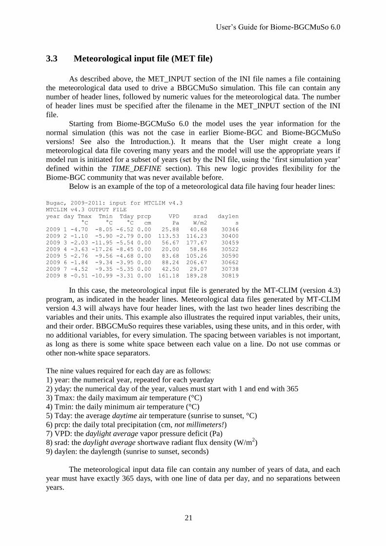
The second required input file is the meteorological data file (MET file). It contains
daily values for air temperature, precipitation, humidity (in terms of daylight vapor pressure
deficit), radiation, and daylength at the simulation site. It can contain any number of data
records. Important note: BBGCMuSo code assumes that all years have 365 days, so
meteorological data files should be edited to remove one day from leap years (we propose to
drop 31 December in the Northern hemisphere). A new feature in BBGCMuSo v6.0 is the
possibility to use data from a truncated (incomplete) year as input data for the last simulation
year. This means that if the User would like to use the model in the current, ongoing year as
the last simulation year, meteorological data can contain data for less than 365 days. In this
case the model estimates the missing meteorological data as the average of the daily data from
the previous years.
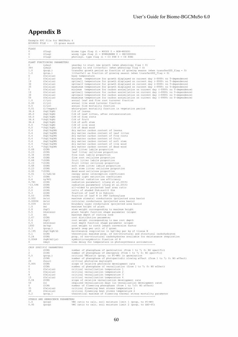
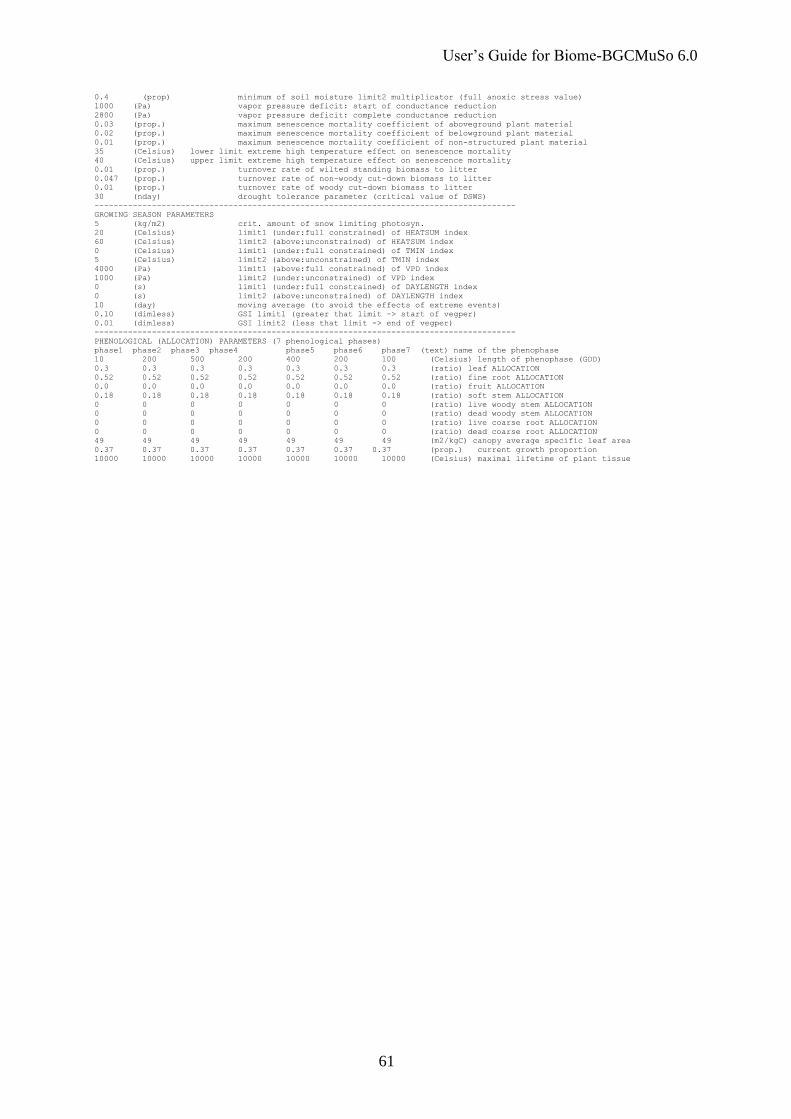
The third required input file is the ecophysiological constants file (EPC file). It
contains an ecophysiological description of the vegetation at a site, including parameters such
as leaf C:N ratio, maximum stomatal conductance, fire and non-fire mortality frequencies,
and allocation ratios. Note that a major re-arrangement of the EPC file was implemented
in Biome-BGCMuSo relative to the earlier versions, so the User should check the proper
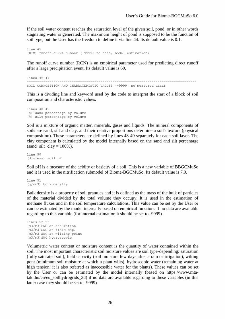
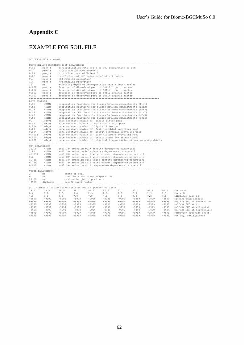
format and content of the EPC file in case of migration from 4.0 or 5.0. The fourth required input file is the soil properties file (SOIL file, having .soi file
extension). It contains the detailed description of the soil at the site, including parameters such
as soil composition, characteristic soil water content values (saturation, field capacity, wilting
point, and hygroscopic water), bulk density, nitrogen cycle related parameters, decomposition
related parameters etc. Some of the parameters were previously included in the EPC file in
v4.0 and v5.0.
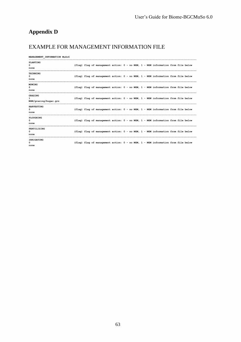
The most important optional input file is the management file (MGM file, having
.mgm file extension) which allows the simulation of different human intervention (mowing,
grazing, sowing, harvest, ploughing, irrigating, fertilizing and thinning).
There are also seven other optional input files: carbon-dioxide file, nitrogen deposition
file, mortality file, stomatal conductance file, groundwater file, onday and offday file (see
below).
The last input file is the special restart file, which is typically the output of the spinup
phase and a necessary input for normal simulation. Detailed description of the files can be
found below.
A NOTE ON USING SPECIAL CHARACTERS IN THE INPUT FILES
For compatibility reasons please do not use non-ASCII characters in your input files!
Furthermore, we strongly recommend using either “\” or either “/” consistently for path
User’s Guide for Biome-BGCMuSo 6.0
9
definition. MS Windows can accept both types, but any other UNIX/UNIX-like systems such
as macOS, Free-BSD or GNU/Linux uses only “/”. For that reason, if it is not inconvenient
for the Windows Users, we recommend to use only “/” for paths. With this little caution your
input files will be portable.
User’s Guide for Biome-BGCMuSo 6.0
10
3.2 Initialization file (INI file)
Below we introduce the structure of the INI file of the model which was substantially
extended in comparison with the Biome-BGC v4.1.1. MPI version. The initialization file is
broken into sections with a keyword starting each new section and a special keyword at the
end of the file. Keywords must be present and should not be removed in any case!
Additionally, please be very careful not to use empty lines inside the sections. This
organization helps to ensure that the proper format for the initialization file is maintained
while editing for new simulations. The order of the sections and the order of the lines within
each section is critical, and changes in order will result in failed or flawed executions. It is
highly recommended that the example INI files be copied to a safe directory for future
reference on proper formatting. There is a fair amount of error checking on the INI file
format, but it is still possible to scramble the order of lines in a way that the program does not
detect. In this case the model will run, but the results will be garbage. Copying the template is
the easiest way to make a new INI file with assurance of the correct format, but remember to
replace ALL of the parameters with those for the new site. It is not necessary to have blank
lines between the end of one section and the keyword for the next section, but keeping them
in makes the INI file more readable.
Each line can contain up to 100 characters of comment information, after a keyword or
after an input parameter (or after more than one input parameter; see below e.g. the soil
texture definition in the SITE block). This information is for your reference in keeping the
correct format in the INI file, and is ignored by the program. Every line is required, even if
flags are set that mean the information on a line will be ignored. The first line of the file is for
header information that helps you keep track of which INI file is for which simulation when
you are doing a sequence of simulations. This line can contain up to 100 characters of
information. There is no keyword for this header line.
The name of the INI files is not fixed. However, we propose to use the following
filename convention. Name your spinup INI file as something_s.ini, and the normal INI file
as something_n.ini where something is arbitrary (note the _s and _n convention!). This
convention can be useful if you plan to use the so-called RBBGCMuSo R tool developed by
our team (https://github.com/hollorol/RBBGCMuso). The work with RBBGCMuSo is much
easier if you follow this convention as it helps the package to automatically identify the
spinup or the normal INI files.
Below we provide examples for the specific sections using Courier New Font. A
complete example INI file is given in Appendix A.
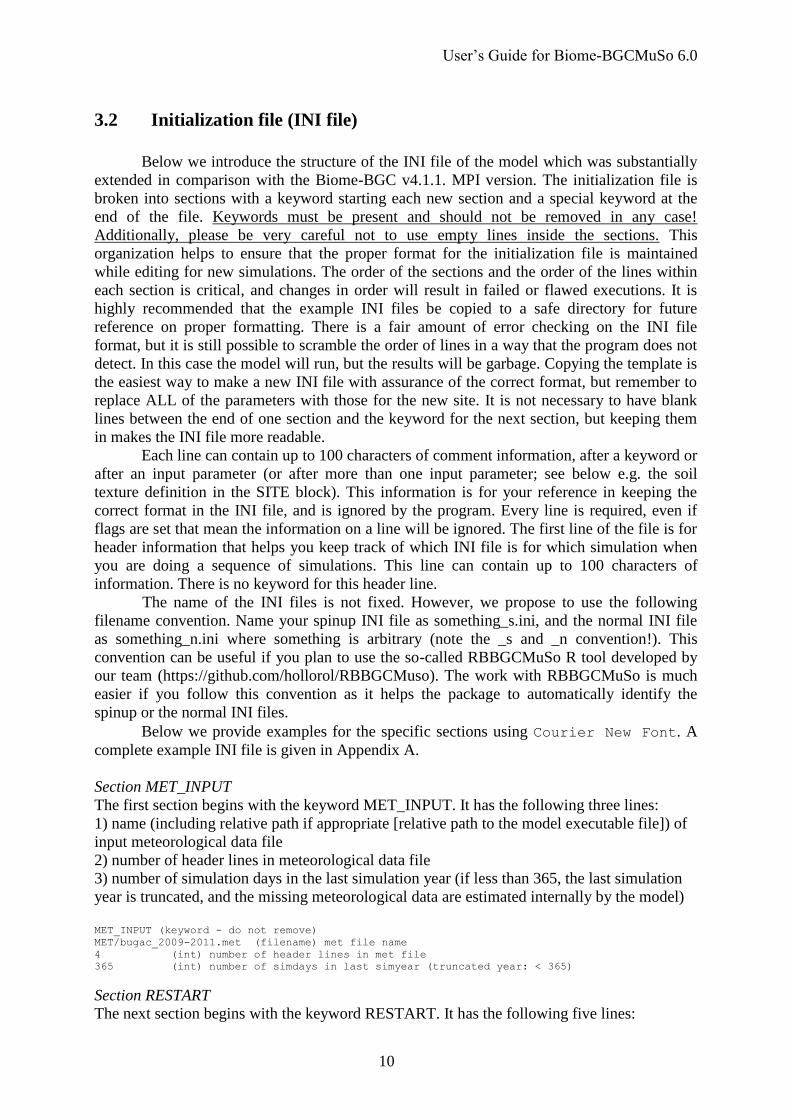
Section MET_INPUT
The first section begins with the keyword MET_INPUT. It has the following three lines:
1) name (including relative path if appropriate [relative path to the model executable file]) of
input meteorological data file
2) number of header lines in meteorological data file
3) number of simulation days in the last simulation year (if less than 365, the last simulation
year is truncated, and the missing meteorological data are estimated internally by the model)
MET_INPUT (keyword - do not remove) MET/bugac_2009-2011.met (filename) met file name 4 (int) number of header lines in met file 365 (int) number of simdays in last simyear (truncated year: < 365)
Section RESTART
The next section begins with the keyword RESTART. It has the following five lines:
User’s Guide for Biome-BGCMuSo 6.0
11
1) flag (1 or 0) for reading (1) or not reading (0) a restart file from the end of a previous
simulation
2) flag (1 or 0) for writing (1) or not writing (0) a restart file at the end of this simulation
3) input restart filename (including path if appropriate)
4) output restart filename (including path if appropriate)
Lines 3) is only relevant when flag in line 1) is set to 1. Line 4) is only relevant when flag in
line 2) is set to 1.
RESTART (keyword - do not remove) 1 (flag) 1: read restart 0: don’t read restart 0 (flag) 1: write restart 0: don’t write restart RST/bugacI.rst (filename) name of the input restart file RST/bugacO.rst (filename) name of the output restart file
Section TIME_DEFINE
The next section begins with the keyword TIME_DEFINE. It has the following five lines:
1) number of years to run for this simulation
2) first simulation year (e.g. 1998)
3) flag (1 or 0) for spinup simulation (1) or normal simulation (0)
4) maximum number of years to run in spinup model
Line 1) should be equal to the number of years of data in meteorological input data file. Line
2) defines the starting point for the simulation output, and is mainly used in the simple text
output file (described below). Line 3) sets the simulation mode for either a spinup run or a
normal run.
If spinup mode is selected, the meteorological data file will be recycled enough times to
establish steady-state conditions in the soil carbon and nitrogen pools. The number of years of
simulation for a spinup run will depend on the climate and vegetation characteristics, but will
not exceed the number of years specified on line 4). If a spinup run reaches the maximum
number of years specified in line 4), it is likely that the resulting final soil carbon and nitrogen
pools are not equilibrated with the climate, usually indicating a long-term net sink of carbon.
This is observed, for example, in some boreal climates, where the model predicts long-term
accumulation of organic matter (peat formation).
TIME_DEFINE (keyword - do not remove) 3 (int) number of simulation years 2009 (int) first simulation year 0 (flag) 1: spinup run 0: normal run 6000 (int) maximum number of spinup years
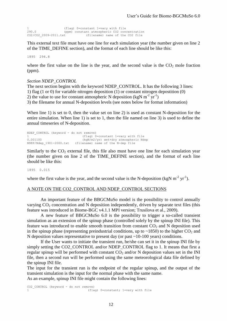
Section CO2_CONTROL
The next section begins with the keyword CO2_CONTROL. It has the following 3 lines:
1) flag (0,1) controlling CO2 concentration: 0=constant, 1=varying using values from an
external file
2) the value to use for constant CO2 concentration (ppm)
3) the filename for annual CO2 levels (see notes below for format information)
When line 1) is set to 0, then the value on line 2) sets the constant CO2 level for the entire
simulation. When line 1) is set to 1, then the file named on line 3) is used to define the annual
timeseries of CO2 concentration.
CO2_CONTROL (keyword - do not remove)
User’s Guide for Biome-BGCMuSo 6.0
12
1 (flag) 0=constant 1=vary with file 290.0 (ppm) constant atmospheric CO2 concentration CO2/CO2_2009-2011.txt (filename) name of the CO2 file
This external text file must have one line for each simulation year (the number given on line 2
of the TIME_DEFINE section), and the format of each line should be like this:
1895 294.8
where the first value on the line is the year, and the second value is the CO2 mole fraction
(ppm).
Section NDEP_CONTROL
The next section begins with the keyword NDEP_CONTROL. It has the following 3 lines:
1) flag (1 or 0) for variable nitrogen deposition (1) or constant nitrogen depostition (0)
2) the value to use for constant atmospheric N deposition (kgN m-2
yr-1
)
3) the filename for annual N-deposition levels (see notes below for format information)
When line 1) is set to 0, then the value set on line 2) is used as constant N-deposition for the
entire simulation. When line 1) is set to 1, then the file named on line 3) is used to define the
annual timeseries of N-deposition.
NDEP_CONTROL (keyword - do not remove) 1 (flag) 0=constant 1=vary with file 0.001100 (kgN/m2/yr) wet+dry atmospheric Ndep NDEP/Ndep_1901-2000.txt (filename) name of the N-dep file
Similarly to the CO2 external file, this file also must have one line for each simulation year
(the number given on line 2 of the TIME_DEFINE section), and the format of each line
should be like this:
1895 0.015
where the first value is the year, and the second value is the N-deposition (kgN m-2
yr-1
).
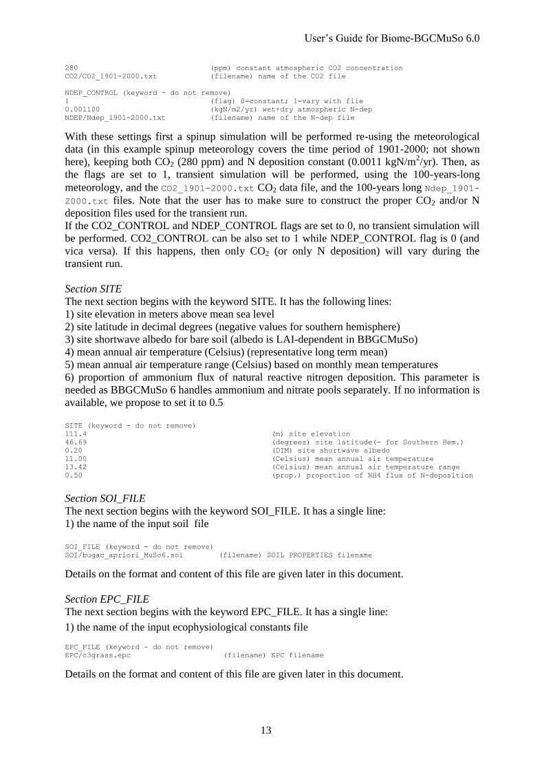
A NOTE ON THE CO2_CONTROL AND NDEP_CONTROL SECTIONS
An important feature of the BBGCMuSo model is the possibility to control annually
varying CO2 concentration and N deposition independently, driven by separate text files (this
feature was introduced in Biome-BGC v4.1.1 MPI version; Trusilova et al., 2009).
A new feature of BBGCMuSo 6.0 is the possibility to trigger a so-called transient
simulation as an extension of the spinup phase (controlled solely by the spinup INI file). This
feature was introduced to enable smooth transition from constant CO2 and N deposition used
in the spinup phase (representing preindustrial conditions, up to ~1850) to the higher CO2 and
N deposition values representative to present day (or past ~10-100 years) conditions.
If the User wants to initiate the transient run, he/she can set it in the spinup INI file by
simply setting the CO2_CONTROL and/or NDEP_CONTROL flag to 1. It means that first a
regular spinup will be performed with constant CO2 and/or N deposition values set in the INI
file, then a second run will be performed using the same meteorological data file defined by
the spinup INI file.
The input for the transient run is the endpoint of the regular spinup, and the output of the
transient simulation is the input for the normal phase with the same name.
As an example, spinup INI file might contain the following lines:
CO2_CONTROL (keyword - do not remove) 1 (flag) 0=constant; 1=vary with file
User’s Guide for Biome-BGCMuSo 6.0
13
280 (ppm) constant atmospheric CO2 concentration CO2/CO2_1901-2000.txt (filename) name of the CO2 file
NDEP_CONTROL (keyword - do not remove) 1 (flag) 0=constant; 1=vary with file 0.001100 (kgN/m2/yr) wet+dry atmospheric N-dep NDEP/Ndep_1901-2000.txt (filename) name of the N-dep file
With these settings first a spinup simulation will be performed re-using the meteorological
data (in this example spinup meteorology covers the time period of 1901-2000; not shown
here), keeping both CO2 (280 ppm) and N deposition constant (0.0011 kgN/m2/yr). Then, as
the flags are set to 1, transient simulation will be performed, using the 100-years-long
meteorology, and the CO2_1901-2000.txt CO2 data file, and the 100-years long Ndep_1901-
2000.txt files. Note that the user has to make sure to construct the proper CO2 and/or N
deposition files used for the transient run.
If the CO2_CONTROL and NDEP_CONTROL flags are set to 0, no transient simulation will
be performed. CO2_CONTROL can be also set to 1 while NDEP_CONTROL flag is 0 (and
vica versa). If this happens, then only CO2 (or only N deposition) will vary during the
transient run.
Section SITE
The next section begins with the keyword SITE. It has the following lines:
1) site elevation in meters above mean sea level
2) site latitude in decimal degrees (negative values for southern hemisphere)
3) site shortwave albedo for bare soil (albedo is LAI-dependent in BBGCMuSo)
4) mean annual air temperature (Celsius) (representative long term mean)
5) mean annual air temperature range (Celsius) based on monthly mean temperatures
6) proportion of ammonium flux of natural reactive nitrogen deposition. This parameter is
needed as BBGCMuSo 6 handles ammonium and nitrate pools separately. If no information is
available, we propose to set it to 0.5
SITE (keyword - do not remove) 111.4 (m) site elevation 46.69 (degrees) site latitude(- for Southern Hem.)
0.20 (DIM) site shortwave albedo
11.00 (Celsius) mean annual air temperature 13.42 (Celsius) mean annual air temperature range
0.50 (prop.) proportion of NH4 flux of N-deposition
Section SOI_FILE
The next section begins with the keyword SOI_FILE. It has a single line:
1) the name of the input soil file
SOI_FILE (keyword - do not remove) SOI/bugac_apriori_MuSo6.soi (filename) SOIL PROPERTIES filename
Details on the format and content of this file are given later in this document.
Section EPC_FILE
The next section begins with the keyword EPC_FILE. It has a single line:
1) the name of the input ecophysiological constants file EPC_FILE (keyword - do not remove) EPC/c3grass.epc (filename) EPC filename
Details on the format and content of this file are given later in this document.
User’s Guide for Biome-BGCMuSo 6.0
14
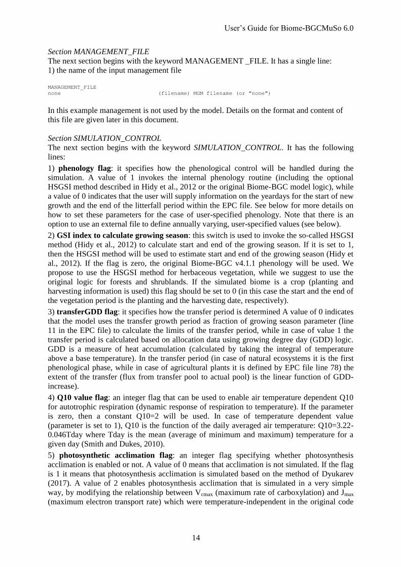
Section MANAGEMENT_FILE
The next section begins with the keyword MANAGEMENT _FILE. It has a single line:
1) the name of the input management file
MANAGEMENT_FILE
none (filename) MGM filename (or "none")
In this example management is not used by the model. Details on the format and content of
this file are given later in this document.
Section SIMULATION_CONTROL
The next section begins with the keyword SIMULATION_CONTROL. It has the following
lines:
1) phenology flag: it specifies how the phenological control will be handled during the
simulation. A value of 1 invokes the internal phenology routine (including the optional
HSGSI method described in Hidy et al., 2012 or the original Biome-BGC model logic), while
a value of 0 indicates that the user will supply information on the yeardays for the start of new
growth and the end of the litterfall period within the EPC file. See below for more details on
how to set these parameters for the case of user-specified phenology. Note that there is an
option to use an external file to define annually varying, user-specified values (see below).
2) GSI index to calculate growing season: this switch is used to invoke the so-called HSGSI
method (Hidy et al., 2012) to calculate start and end of the growing season. If it is set to 1,
then the HSGSI method will be used to estimate start and end of the growing season (Hidy et
al., 2012). If the flag is zero, the original Biome-BGC v4.1.1 phenology will be used. We
propose to use the HSGSI method for herbaceous vegetation, while we suggest to use the
original logic for forests and shrublands. If the simulated biome is a crop (planting and
harvesting information is used) this flag should be set to 0 (in this case the start and the end of
the vegetation period is the planting and the harvesting date, respectively).
3) transferGDD flag: it specifies how the transfer period is determined A value of 0 indicates
that the model uses the transfer growth period as fraction of growing season parameter (line
11 in the EPC file) to calculate the limits of the transfer period, while in case of value 1 the
transfer period is calculated based on allocation data using growing degree day (GDD) logic.
GDD is a measure of heat accumulation (calculated by taking the integral of temperature
above a base temperature). In the transfer period (in case of natural ecosystems it is the first
phenological phase, while in case of agricultural plants it is defined by EPC file line 78) the
extent of the transfer (flux from transfer pool to actual pool) is the linear function of GDD-
increase).
4) Q10 value flag: an integer flag that can be used to enable air temperature dependent Q10
for autotrophic respiration (dynamic response of respiration to temperature). If the parameter
is zero, then a constant Q10=2 will be used. In case of temperature dependent value
(parameter is set to 1), Q10 is the function of the daily averaged air temperature: Q10=3.22-
0.046Tday where Tday is the mean (average of minimum and maximum) temperature for a
given day (Smith and Dukes, 2010).
5) photosynthetic acclimation flag: an integer flag specifying whether photosynthesis
acclimation is enabled or not. A value of 0 means that acclimation is not simulated. If the flag
is 1 it means that photosynthesis acclimation is simulated based on the method of Dyukarev
(2017). A value of 2 enables photosynthesis acclimation that is simulated in a very simple
way, by modifying the relationship between Vcmax (maximum rate of carboxylation) and Jmax
(maximum electron transport rate) which were temperature-independent in the original code
User’s Guide for Biome-BGCMuSo 6.0
15
(Kattge and Knorr, 2007). Temperature dependency is calculated based on average
temperature for the previous 30 days.
6) respiration acclimation flag: an integer flag specifying whether maintenance respiration
acclimation is enabled or not. A value of 0 means that acclimation is not simulated. If the flag
is 1 it means that acclimation is simulated. Respiration acclimation is calculated after Tjoelker
et al. (2001) and Smith and Dukes (2013). In this routine adjustment of respiration is
calculated based on the mean air temperature of the previous 10 days.
7) CO2 conductance reduction flag: specifying whether stomatal conductance should be
affected by changing atmospheric CO2 concentration or not (Franks et al., 2013). We
recommend setting this flag to 1.
8) soil temperature calculation flag: specifying the soil temperature calculation method. 0
invokes the Zheng et al. (1993) based method with logarithmic downward dampening of
temperature fluctuations within the soil. 1 means that the empirical method of DSSAT/4M
(Sándor and Fodor, 2012) will be used. The preferred method should be selected based on
comparison with measurements at the specific site (if available).
9) soil water calculation flag: specifying the soil water balance calculation method. 0 means
that soil water balance is simulated based on the Richards equation, while 1 means that the so-
called tipping bucket method is used. For details see Hidy et al. (2016). There is no
recommended value for this flag; the User has the freedom to test both methods and use the
most appropriate based on comparison with measured data.
10) discretization level of SWC calculation flag: specifying the discretization level of soil
water balance calculation method (in case of Richards method). 0 means low, 1 means
medium, while 2 means high accuracy of the finite difference method used for soil water
balance. Level 0 is the fastest, level 2 is the slowest. We propose to use level 0 for everyday
simulation. It is only applicable in case of the Richards-equation based water balance method
(if flag is 0 in line 9).
11) photosynthesis calculation flag: specifying the photosynthesis calculation method. 0
means that photosynthesis is simulated based on the Farquhar-method (which was the original
method in Biome-BGC), while 1 means that the method of the DSSAT model is used (that is
a simple light use efficiency model). There is no recommended value for this flag; the User
has the freedom to test both methods and use the most appropriate based on comparison with
measured data.
12) evapotranspiration calculation flag: specifying the evapotranspiration (ET) calculation
method. 0 means that ET is simulated based on the Penman-Monteith method (original model
logic), while 1 means simulation based on the Pristley-Taylor method. NOTE THAT IN THE
CURRENT MODEL VERSION ONLY THE PENMAN-MONTEITH METHOD IS
IMPLEMENTED, SO THE FLAG MUST BE SET TO NIL. The Pristley-Taylor method will
be implemented in forthcoming model versions.
13) radiation calculation flag: it specifies the radiation calculation method. 0 means that
within the ET routine absorbed shortwave radiation drives ET, while 1 means that the
internally calculated net radiation (Rn) drives the ET routine. There is no recommended value
for this flag; the User has the freedom to test both methods and use the most appropriate
based on comparison with measured data.
14) soilstress calculation method: it specifies the soil moisture stress calculation method. 0
means that soil water stress is based on difference between the actual and the characteristic
soil water content values, while 1 means that stress is based on transpiration demand.
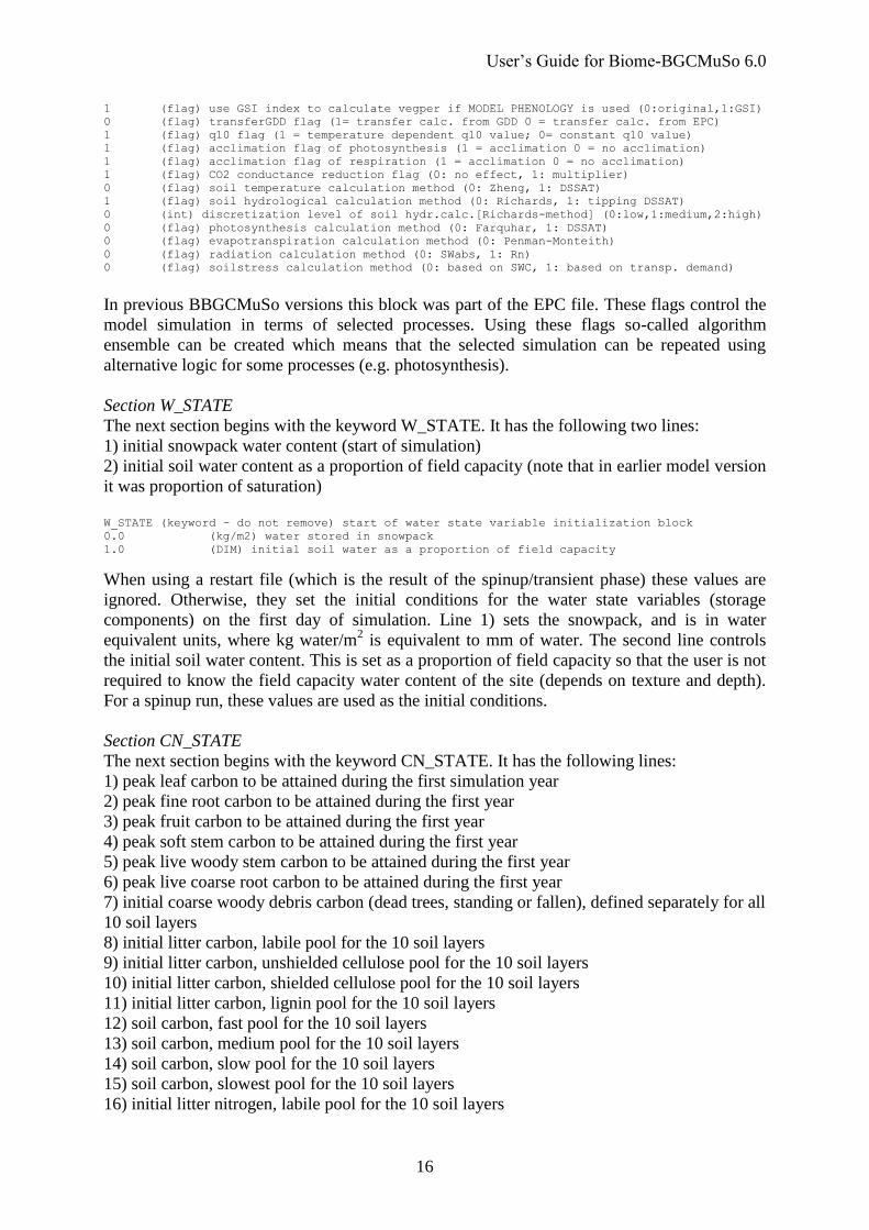
SIMULATION_CONTROL
1 (flag) phenology flag (1 = MODEL PHENOLOGY 0 = USER-SPECIFIED PHENOLOGY)
User’s Guide for Biome-BGCMuSo 6.0
16
1 (flag) use GSI index to calculate vegper if MODEL PHENOLOGY is used (0:original,1:GSI)
0 (flag) transferGDD flag (1= transfer calc. from GDD 0 = transfer calc. from EPC)
1 (flag) q10 flag (1 = temperature dependent q10 value; 0= constant q10 value)
1 (flag) acclimation flag of photosynthesis (1 = acclimation 0 = no acclimation)
1 (flag) acclimation flag of respiration (1 = acclimation 0 = no acclimation)
1 (flag) CO2 conductance reduction flag (0: no effect, 1: multiplier)
0 (flag) soil temperature calculation method (0: Zheng, 1: DSSAT)
0 (flag) soilstress calculation method (0: based on SWC, 1: based on transp. demand)
In previous BBGCMuSo versions this block was part of the EPC file. These flags control the
model simulation in terms of selected processes. Using these flags so-called algorithm
ensemble can be created which means that the selected simulation can be repeated using
alternative logic for some processes (e.g. photosynthesis).
Section W_STATE
The next section begins with the keyword W_STATE. It has the following two lines:
1) initial snowpack water content (start of simulation)
2) initial soil water content as a proportion of field capacity (note that in earlier model version
it was proportion of saturation)
W_STATE (keyword – do not remove) start of water state variable initialization block 0.0 (kg/m2) water stored in snowpack 1.0 (DIM) initial soil water as a proportion of field capacity
When using a restart file (which is the result of the spinup/transient phase) these values are
ignored. Otherwise, they set the initial conditions for the water state variables (storage
components) on the first day of simulation. Line 1) sets the snowpack, and is in water
equivalent units, where kg water/m2 is equivalent to mm of water. The second line controls
the initial soil water content. This is set as a proportion of field capacity so that the user is not
required to know the field capacity water content of the site (depends on texture and depth).
For a spinup run, these values are used as the initial conditions.
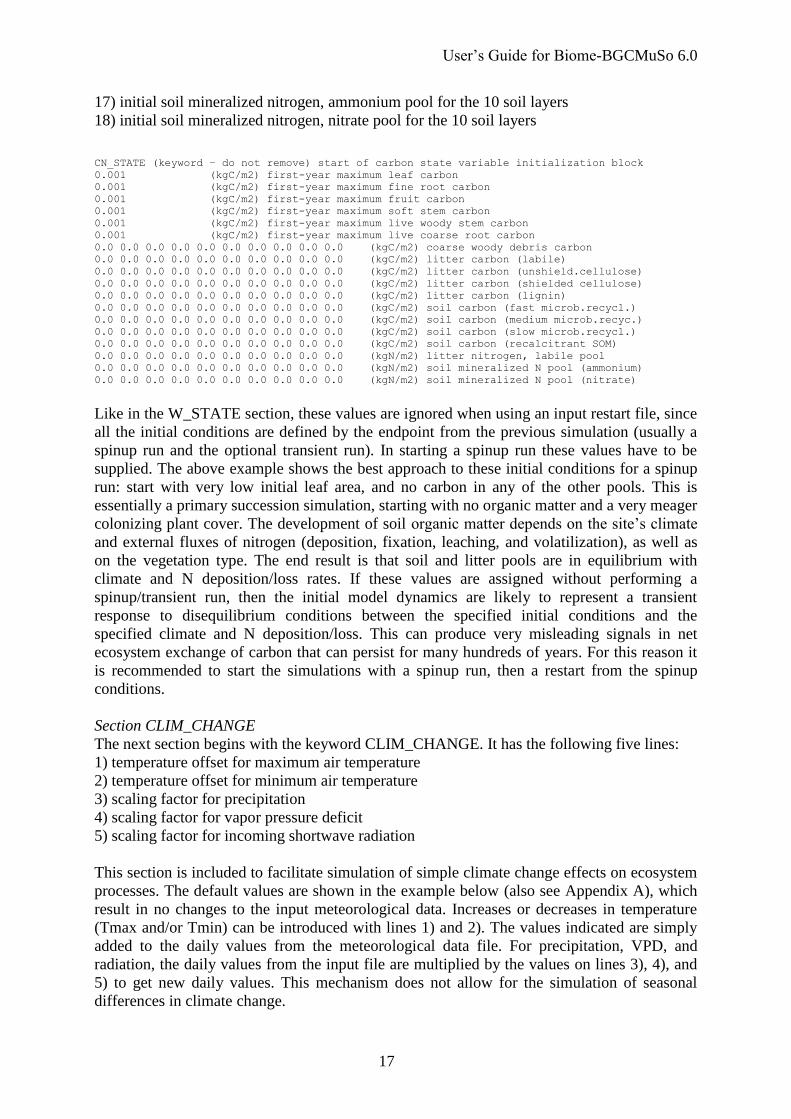
Section CN_STATE
The next section begins with the keyword CN_STATE. It has the following lines:
1) peak leaf carbon to be attained during the first simulation year
2) peak fine root carbon to be attained during the first year
3) peak fruit carbon to be attained during the first year
4) peak soft stem carbon to be attained during the first year
5) peak live woody stem carbon to be attained during the first year
6) peak live coarse root carbon to be attained during the first year
7) initial coarse woody debris carbon (dead trees, standing or fallen), defined separately for all
10 soil layers
8) initial litter carbon, labile pool for the 10 soil layers
9) initial litter carbon, unshielded cellulose pool for the 10 soil layers
10) initial litter carbon, shielded cellulose pool for the 10 soil layers
11) initial litter carbon, lignin pool for the 10 soil layers
12) soil carbon, fast pool for the 10 soil layers
13) soil carbon, medium pool for the 10 soil layers
14) soil carbon, slow pool for the 10 soil layers
15) soil carbon, slowest pool for the 10 soil layers
16) initial litter nitrogen, labile pool for the 10 soil layers
User’s Guide for Biome-BGCMuSo 6.0
17
17) initial soil mineralized nitrogen, ammonium pool for the 10 soil layers
18) initial soil mineralized nitrogen, nitrate pool for the 10 soil layers
Like in the W_STATE section, these values are ignored when using an input restart file, since
all the initial conditions are defined by the endpoint from the previous simulation (usually a
spinup run and the optional transient run). In starting a spinup run these values have to be
supplied. The above example shows the best approach to these initial conditions for a spinup
run: start with very low initial leaf area, and no carbon in any of the other pools. This is
essentially a primary succession simulation, starting with no organic matter and a very meager
colonizing plant cover. The development of soil organic matter depends on the site’s climate
and external fluxes of nitrogen (deposition, fixation, leaching, and volatilization), as well as
on the vegetation type. The end result is that soil and litter pools are in equilibrium with
climate and N deposition/loss rates. If these values are assigned without performing a
spinup/transient run, then the initial model dynamics are likely to represent a transient
response to disequilibrium conditions between the specified initial conditions and the
specified climate and N deposition/loss. This can produce very misleading signals in net
ecosystem exchange of carbon that can persist for many hundreds of years. For this reason it
is recommended to start the simulations with a spinup run, then a restart from the spinup
conditions.
Section CLIM_CHANGE
The next section begins with the keyword CLIM_CHANGE. It has the following five lines:
1) temperature offset for maximum air temperature
2) temperature offset for minimum air temperature
3) scaling factor for precipitation
4) scaling factor for vapor pressure deficit
5) scaling factor for incoming shortwave radiation
This section is included to facilitate simulation of simple climate change effects on ecosystem
processes. The default values are shown in the example below (also see Appendix A), which
result in no changes to the input meteorological data. Increases or decreases in temperature
(Tmax and/or Tmin) can be introduced with lines 1) and 2). The values indicated are simply
added to the daily values from the meteorological data file. For precipitation, VPD, and
radiation, the daily values from the input file are multiplied by the values on lines 3), 4), and
5) to get new daily values. This mechanism does not allow for the simulation of seasonal
differences in climate change.
User’s Guide for Biome-BGCMuSo 6.0
18
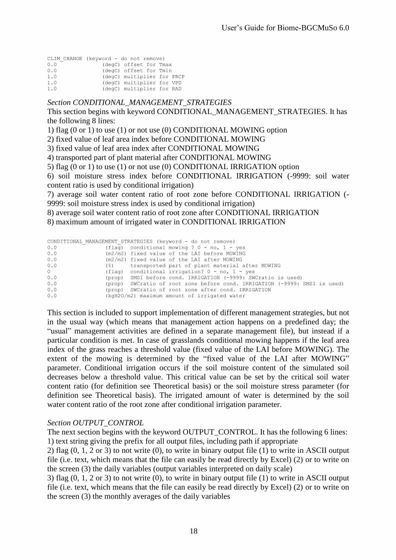
CLIM_CHANGE (keyword - do not remove) 0.0 (degC) offset for Tmax 0.0 (degC) offset for Tmin 1.0 (degC) multiplier for PRCP 1.0 (degC) multiplier for VPD 1.0 (degC) multiplier for RAD
Section CONDITIONAL_MANAGEMENT_STRATEGIES
This section begins with keyword CONDITIONAL_MANAGEMENT_STRATEGIES. It has
the following 8 lines:
1) flag (0 or 1) to use (1) or not use (0) CONDITIONAL MOWING option
2) fixed value of leaf area index before CONDITIONAL MOWING
3) fixed value of leaf area index after CONDITIONAL MOWING
4) transported part of plant material after CONDITIONAL MOWING
5) flag (0 or 1) to use (1) or not use (0) CONDITIONAL IRRIGATION option
6) soil moisture stress index before CONDITIONAL IRRIGATION (-9999: soil water
content ratio is used by conditional irrigation)
7) average soil water content ratio of root zone before CONDITIONAL IRRIGATION (-
9999: soil moisture stress index is used by conditional irrigation)
8) average soil water content ratio of root zone after CONDITIONAL IRRIGATION
8) maximum amount of irrigated water in CONDITIONAL IRRIGATION
CONDITIONAL_MANAGEMENT_STRATEGIES (keyword - do not remove) 0.0 (flag) conditional mowing ? 0 - no, 1 - yes
0.0 (m2/m2) fixed value of the LAI before MOWING
0.0 (m2/m2) fixed value of the LAI after MOWING
0.0 (%) transported part of plant material after MOWING
0 (flag) conditional irrigation? 0 - no, 1 - yes
0.0 (prop) SMSI before cond. IRRIGATION (-9999: SWCratio is used)
0.0 (prop) SWCratio of root zone before cond. IRRIGATION (-9999: SMSI is used)
0.0 (prop) SWCratio of root zone after cond. IRRIGATION
0.0 (kgH2O/m2) maximum amount of irrigated water
This section is included to support implementation of different management strategies, but not
in the usual way (which means that management action happens on a predefined day; the
“usual” management activities are defined in a separate management file), but instead if a
particular condition is met. In case of grasslands conditional mowing happens if the leaf area
index of the grass reaches a threshold value (fixed value of the LAI before MOWING). The
extent of the mowing is determined by the “fixed value of the LAI after MOWING”
parameter. Conditional irrigation occurs if the soil moisture content of the simulated soil
decreases below a threshold value. This critical value can be set by the critical soil water
content ratio (for definition see Theoretical basis) or the soil moisture stress parameter (for
definition see Theoretical basis). The irrigated amount of water is determined by the soil
water content ratio of the root zone after conditional irrigation parameter.
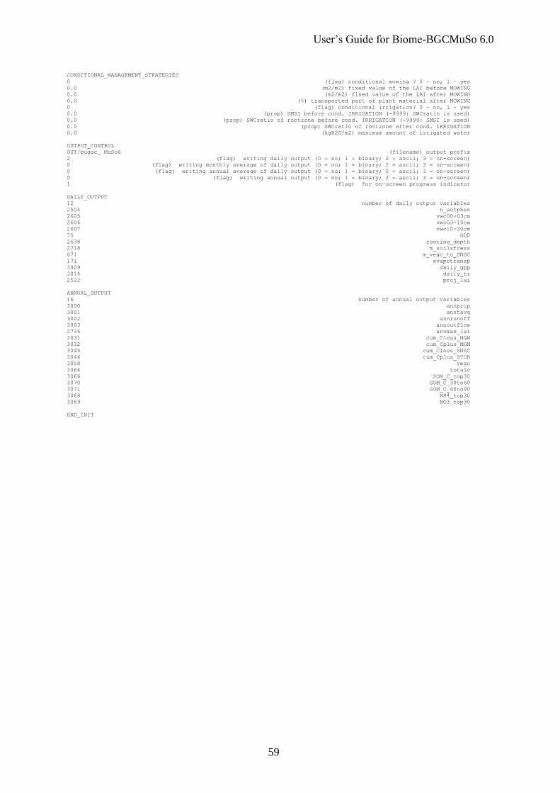
Section OUTPUT_CONTROL
The next section begins with the keyword OUTPUT_CONTROL. It has the following 6 lines:
1) text string giving the prefix for all output files, including path if appropriate
2) flag (0, 1, 2 or 3) to not write (0), to write in binary output file (1) to write in ASCII output
file (i.e. text, which means that the file can easily be read directly by Excel) (2) or to write on
the screen (3) the daily variables (output variables interpreted on daily scale)
3) flag (0, 1, 2 or 3) to not write (0), to write in binary output file (1) to write in ASCII output
file (i.e. text, which means that the file can easily be read directly by Excel) (2) or to write on
the screen (3) the monthly averages of the daily variables
User’s Guide for Biome-BGCMuSo 6.0
19
4 flag (0, 1, 2 or 3) to not write (0), to write in binary output file (1) to write in ASCII output
file (i.e. text, which means that the file can easily be read directly by Excel) (2) or to write on
the screen (3) the annual averages of the daily variables
5) flag (0, 1, 2 or 3) to not write (0), to write in binary output file (1) to write in ASCII output
file (with .txt extension, which means that the file can easily be read directly by any text
editor like Notepad, EditPad Lite, and even with Excel) (2) or to write on the screen (3) the
annual variables (output variables interpreted on annual scale)
6) flag (1 or 0) to send (1) or not send (0) simulation progress information to the screen
OUTPUT_CONTROL (keyword - do not remove) outputs/bugac_apriori_MuSo6 (filename) output prefix 1 (flag) writing daily output (0 = no; 1 = binary; 2 = ascii) 0 (flag) writing monthly average of daily output (0=no; 1=binary; 2=ascii) 0 (flag) writing annual average of daily output (0=no; 1=binary; 2=ascii)
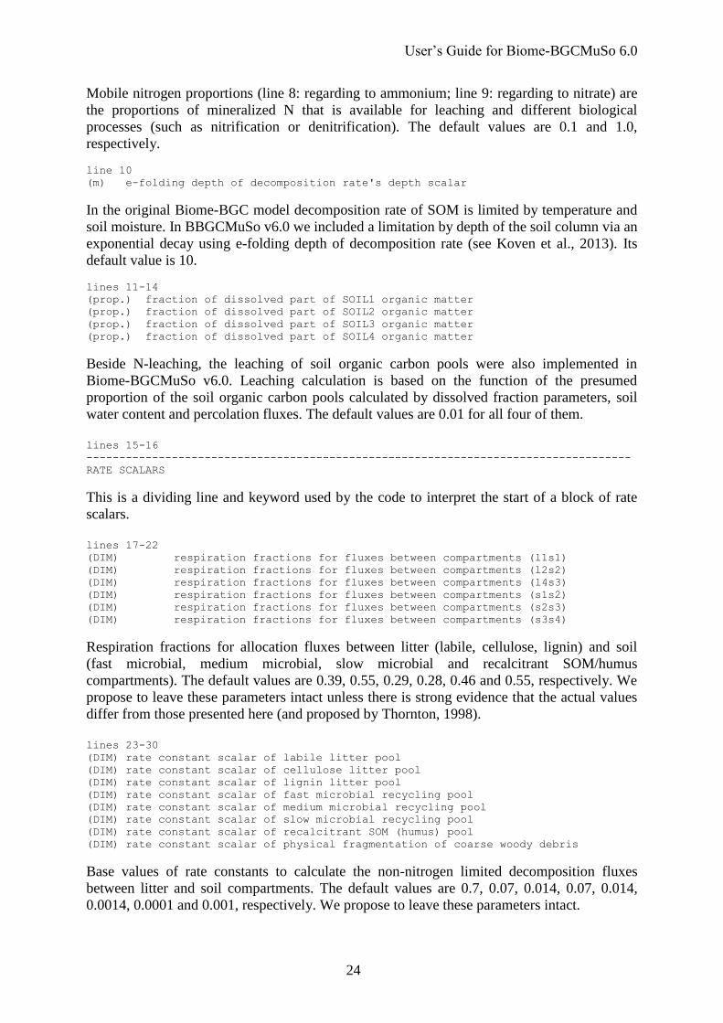
Mobile nitrogen proportions (line 8: regarding to ammonium; line 9: regarding to nitrate) are
the proportions of mineralized N that is available for leaching and different biological
processes (such as nitrification or denitrification). The default values are 0.1 and 1.0,
respectively.
line 10 (m) e-folding depth of decomposition rate's depth scalar
In the original Biome-BGC model decomposition rate of SOM is limited by temperature and
soil moisture. In BBGCMuSo v6.0 we included a limitation by depth of the soil column via an
exponential decay using e-folding depth of decomposition rate (see Koven et al., 2013). Its
default value is 10.
lines 11-14 (prop.) fraction of dissolved part of SOIL1 organic matter (prop.) fraction of dissolved part of SOIL2 organic matter (prop.) fraction of dissolved part of SOIL3 organic matter (prop.) fraction of dissolved part of SOIL4 organic matter
Beside N-leaching, the leaching of soil organic carbon pools were also implemented in
Biome-BGCMuSo v6.0. Leaching calculation is based on the function of the presumed
proportion of the soil organic carbon pools calculated by dissolved fraction parameters, soil
water content and percolation fluxes. The default values are 0.01 for all four of them.
This is a dividing line and keyword used by the code to interpret the start of a block of rate
scalars.
lines 17-22 (DIM) respiration fractions for fluxes between compartments (l1s1) (DIM) respiration fractions for fluxes between compartments (l2s2) (DIM) respiration fractions for fluxes between compartments (l4s3) (DIM) respiration fractions for fluxes between compartments (s1s2) (DIM) respiration fractions for fluxes between compartments (s2s3) (DIM) respiration fractions for fluxes between compartments (s3s4)
Respiration fractions for allocation fluxes between litter (labile, cellulose, lignin) and soil
(fast microbial, medium microbial, slow microbial and recalcitrant SOM/humus
compartments). The default values are 0.39, 0.55, 0.29, 0.28, 0.46 and 0.55, respectively. We
propose to leave these parameters intact unless there is strong evidence that the actual values
differ from those presented here (and proposed by Thornton, 1998).
lines 23-30 (DIM) rate constant scalar of labile litter pool (DIM) rate constant scalar of cellulose litter pool (DIM) rate constant scalar of lignin litter pool (DIM) rate constant scalar of fast microbial recycling pool (DIM) rate constant scalar of medium microbial recycling pool (DIM) rate constant scalar of slow microbial recycling pool (DIM) rate constant scalar of recalcitrant SOM (humus) pool (DIM) rate constant scalar of physical fragmentation of coarse woody debris
Base values of rate constants to calculate the non-nitrogen limited decomposition fluxes
between litter and soil compartments. The default values are 0.7, 0.07, 0.014, 0.07, 0.014,
0.0014, 0.0001 and 0.001, respectively. We propose to leave these parameters intact.
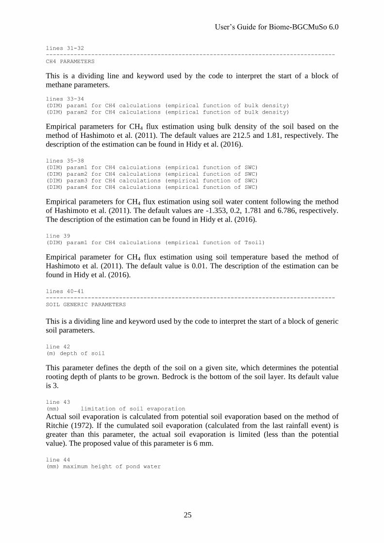
This is a dividing line and keyword used by the code to interpret the start of a block of
methane parameters.
lines 33-34 (DIM) param1 for CH4 calculations (empirical function of bulk density) (DIM) param2 for CH4 calculations (empirical function of bulk density)
Empirical parameters for CH4 flux estimation using bulk density of the soil based on the
method of Hashimoto et al. (2011). The default values are 212.5 and 1.81, respectively. The
description of the estimation can be found in Hidy et al. (2016).
lines 35-38 (DIM) param1 for CH4 calculations (empirical function of SWC) (DIM) param2 for CH4 calculations (empirical function of SWC) (DIM) param3 for CH4 calculations (empirical function of SWC) (DIM) param4 for CH4 calculations (empirical function of SWC)
Empirical parameters for CH4 flux estimation using soil water content following the method
of Hashimoto et al. (2011). The default values are -1.353, 0.2, 1.781 and 6.786, respectively.
The description of the estimation can be found in Hidy et al. (2016).
line 39 (DIM) param1 for CH4 calculations (empirical function of Tsoil)
Empirical parameter for CH4 flux estimation using soil temperature based the method of
Hashimoto et al. (2011). The default value is 0.01. The description of the estimation can be
This is a dividing line and header to indicate the start the PLANT FUNCTIONING
PARAMETERS block.
lines 9-10 (yday) yearday to start new growth (when phenology flag=0) (yday) yearday to end litterfall (when phenology flag=0)
Two integers specifying the day of year for the start of new leaf growth, and the day of year
for the end of the litterfall season, respectively. Relevant only when the phenology flag is 0
(see above line 1 in SIMULATION_CONTROL block of INI file). There are several
important notes about setting these values. To suppress new leaf growth entirely, for example
in the case of a simulation concerned with bare soil processes, set both of these values to
-9999.
Yearday values for these parameters start at 0 and go to 364. Note that BBGCMuSo does not
accept leap-years, i.e. all years are by definition 365 days long.
Northern and Southern hemisphere yeardays are treated differently for these parameters. In
the northern hemisphere, yearday 0 is 1 January, while in the southern hemisphere yearday 0
is 1 July1. This allows the same yearday values to be used to specify deciduous growth habit
in the northern and southern temperate zones.
If the leaf habit flag is set to evergreen (line 5 is set to1) or in case of crop simulation
(planting and harvest is defined in management section – see below), the phenology model
flag in the INI file is assumed to set to user-specified (0), so these values do not have any
effect.
lines 11 and 12 (prop.) transfer growth period as fraction of growing season (prop.) litterfall as fraction of growing season
These two parameters determine the duration of the transfer growth and litterfall periods, and
are defined as proportions of the period between the start of new growth and the end of
litterfall. It is important to keep in mind that if transferGDD flag (see above line 3 in
SIMULATION_CONTROL block of INI file) is set to 1, allocation parameters are used to
determine transfer period, which means that these parameters have no effect on the
simulation! In other cases, these parameters must be set by the user regardless of whether
internal model phenology or user-specified phenology is specified in the phenology model
flag of the INI file. These parameters can take any values from 0.0 to 1.0, where a value of 0.0
indicates that all transfer growth or all litterfall occurs in a single day, and a value of 1.0
indicates that transfer growth or litterfall occur throughout the growing season. Transfer
growth is the growth derived from carbon and nitrogen resources (i.e. non-structural
carbohydrate) stored over the course of the previous growing season. It is the growth that
produces the first flush of new leaves in the spring for deciduous plants. NOTE that when the
User’s Guide for Biome-BGCMuSo 6.0
30
leaf habit flag is set for evergreen, both transfer growth and litterfall are assumed to occur at
constant rates throughout the year, and the specification of these two parameters has no effect.
line 13 (Celsius) base temperature
This parameter sets the base temperature for plant processes. In general, base temperature is
defined as the lowest air temperature where metabolic processes may result in a net substance
gain in aboveground biomass (leaves or stem). (Note that the model does not simulate leaf
temperature, only air and soil temperature are used in model calculations.) Base temperature
is used to calculate a special growing season index (HSGSI; Hidy et al., 2016) to estimate the
start and the end of the vegetation period (Hidy et al., 2012) and to calculate growing degree-
day to estimate the phenological phases and genetically programmed senescence.
lines 14 and 17 (°C) minimum temperature for growth displayed on current day (-9999: no T-depend.) (°C) optimal1 temperature for growth displayed on current day (-9999: no T-depend.) (°C) optimal2 temperature for growth displayed on current day (-9999: no T-depend.)
(°C) maximum temperature for growth displayed on current day (-9999: no T-depend.)
These four parameters set specific thresholds to control air temperature dependency of
allocation. The temperature dependence of allocation is controlled by a ramp function, with a
plateau as optimum. Optimal1 temperature is the smaller temperature when the optimum is
reached (optimum means that the function reaches 1). Optimal2 temperature is the highest
temperature when the optimum ends and the function starts to decrease. Between minimum
and optimal1 temperatures the proportion of growth displayed on current day increases, while
between optimal2 and maximum temperature it decreases linearly from zero to 1 and from 1
to zero, respectively. Below minimum temperature (line 14) and above maximum temperature
(line 17) the proportion of growth displayed on the current day is zero (all the daily
production (i.e. assimilation) goes to the non-structural plant pool, which is represented by the
storage pool in the model; for details about changes in the non-structural carbohydrate pool
simulation logic see Theoretical basis of MuSo6; in prep.). Note that all or none of the four
parameters driving temperature dependency for growth should be set by the User. Also note
that temperature dependence for allocation is an experimental feature of the model, and
should not be used in typical simulations. Setting all four parameters to -9999 disables the
temperature dependency of allocation which means that the original model logic is used.
lines 18 and 21 (°C) min. temperature for C-assimilation displayed on current day (-9999: no limit) (°C) opt1 temperature for C-assimilation displayed on current day (-9999: no limit) (°C) opt2 temperature for C-assimilation displayed on current day (-9999: no limit)
(°C) max. temperature for C-assimilation displayed on current day (-9999: no limit)
These four parameters set optional thresholds on the temperature dependency of carbon
assimilation (photosynthesis). If these thresholds are set, the temperature dependence of C-
assimilation is controlled by a ramp function, with a plateau as optimum. Optimal1
temperature is the smaller temperature when the optimum is reached (equals 1). Optimal2
temperature is the highest temperature when the optimum ends and starts to decrease from 1
to 0. Between minimum and optimal1 temperatures the limitation of carbon assimilation on
current day increases, between optimal2 and maximum temperature it decreases linearly from
zero to 1 and from 1 to zero, respectively. Below minimum temperature and above maximum
temperature thresholds set by the parameters the carbon assimilation is fully downregulated
by the model, so the daily gross primary production is zero on the given day. Note that all or
none of the temperature dependency parameters should be set by the User. Setting all four
User’s Guide for Biome-BGCMuSo 6.0
31
parameters to -9999 disables this additional temperature dependency of assimilation which
means that the original model logic is used. Note that the Farquhar photosynthesis routine has
inherent temperature dependency in the original model. These four parameters were
introduced to set further temperature control on assimilation, to simulate the observed
downregulation of photosynthesis at high temperatures for some biomes. We propose that
first the high temperature effect should be tested by the User (minimum temperature and
optimum1 should be set to e.g. zero in this case). The low temperature related downregulation
is just a possibility that might not be used at all.
line 22 (1/yr) annual leaf and fine root turnover fraction
Determines leaf and fine root turnover for evergreen plants. This is the fraction of the annual
maximum leaf and fine root mass that will be dropped in the following year as litter. It is the
reciprocal of the leaf longevity, so a plant that retains its leaves an average of two years would
have a leaf/fine root turnover of 0.5. Note that leaf and fine root phenology are assumed to be
entirely synchronized for all vegetation types. Also note that when the leaf habit is specified
as deciduous, this parameter is always assumed to be 1.0, and will be reset inside the code if
the User specifies any other value.
line 23 (1/yr) annual live wood turnover fraction
Determines livewood turnover to deadwood for all woody types (deciduous and evergreen).
Important note about the definition of livewood and deadwood in BBGCMuSo: livewood is
defined as the actively respiring woody tissue, that is, the lateral sheathing meristem of
phloem tissue, plus any ray parenchyma extending radially into the xylem tissue. Deadwood
consists of all the other woody material, including the heartwood, the xylem, and the bark. It
has been common in many tree models, including previous versions of Biome-BGC, to divide
the woody tissue into two compartments called "sapwood" and "heartwood", where sapwood
is usually defined as the sum of phloem and xylem, with heartwood defined as the non-
conducting woody tissue. The current treatment ignores the distinction between water-
conducting xylem and non-conducting heartwood.
For herbaceous vegetation the wood related parameters does not affect the simulation.
line 24 (1/yr) annual fire mortality fraction
This parameter specifies the fraction of plant pools subject to fire, on average, each year. The
current treatment ignores the timing of individual fire events, taking a long-term view of the
fire process, in which some fraction of the community is subject to fire each year, at a rate
commensurate with the long-term fire frequency. For example, in a system with a stand-
replacing fire return interval of 100 years, this parameter would be set to 0.01.
line 25 (1/vegper) annual whole-plant mortality fraction
This parameter specifies the fraction of all plant pools that will be removed and sent to the
litter compartments over the course of the vegetation period (from onday to offday). In case of
woodlands, this is one mechanism by which woody material (live and dead) leaves the plant
pool and enters the litter pools to be made available for subsequent decomposition. It is the
conceptual equivalent of wind-throw (but not exclusively, as diseases, competetive processes
in early development phase or frost damage can also cause mortality of plants), and all plant
pools, living and dead, are attenuated at the same rate. This proportion related to the whole
User’s Guide for Biome-BGCMuSo 6.0
32
vegetation period is converted internally to a daily rate, and whole-plant mortality is assumed
to go on at a constant rate throughout the vegetation period. Note that in original Biome-BGC
and in the earlier versions of BBGCMuSo whole plant mortality parameter was related to the
whole year. BBGCMuSo has other mechanism for plant mortality, not present in previous
versions of Biome-BGC. For example, drought related leaf senescence acts together with
annual whole-plant mortality, if applicable. Also, gentically programmed leaf senescence
(which is another option in BBGCMuSo) can also cause leaf mortality besides this daily fixed
plant mortality. In BBGCMuSo annually varying whole-plant mortality fraction can also be
set by providing an external file (see later in this manual). In this case the external data
overrides this setting in the EPC file.
line 26 (kgC/kgN) C:N of leaves
Mass ratio of carbon:nitrogen in live leaves. Note that this is one of the most important
parameters of the model, so its value should be set by the User with caution. Consider using
parameter optimization procedure (like the RBBGCMuSo R package developed by our group)
to set this parameter properly.
line 27 (kgC/kgN) C:N of leaf litter, after retranslocation
Mass ratio of carbon:nitrogen in freshly fallen leaf litter. This can only be higher than or equal
to the C:N for live leaves, i.e. retranslocation can only be positive or zero. Retranslocation is
the removal of nitrogen from the leaves prior to litterfall. The model does not consider the
possibility of retranslocation of carbon out of leaves prior to litterfall.
line 28 (kgC/kgN) C:N of fine roots
Mass ratio of carbon:nitrogen in fine roots. The model assumes that there is no retranslocation
of nitrogen out of fine roots prior to litterfall, so this is the only C:N parameter for fine roots.
This should be equal or greater than the C:N for leaf.
line 29 (kgC/kgN) C:N of fruit
Mass ratio of carbon:nitrogen in fruit. The model assumes that there is no retranslocation of
nitrogen out of fruit prior to litterfall. Fruit C:N ratio should be equal or greater than the C:N
for leaf.
line 30 (kgC/kgN) C:N of soft stem
Mass ratio of carbon:nitrogen in soft stem. The model assumes that there is no retranslocation
of nitrogen out of soft stem prior to litterfall, so this is the only C:N parameter for soft stem.
This should be equal or greater than the C:N for leaf. Soft stem is not present for woody
vegetation.
line 31 (kgC/kgN) C:N of live wood
Mass ratio of carbon:nitrogen for live wood (phloem and ray parenchyma). This will typically
be a much smaller value than the average C:N for all woody parts, and is typically found to be
User’s Guide for Biome-BGCMuSo 6.0
33
close to that for fine roots. As we noted, in case of herbaceous vegetation the wood related
parameters does not affect the simulation.
line 32 (kgC/kgN) C:N of dead wood
Mass ratio of carbon:nitrogen for dead wood (bark, xylem, heartwood). This should be equal
or greater than the C:N for live wood.
lines 33-39
0.4 (kgC/kgDM) dry matter carbon content of leaves
0.4 (kgC/kgDM) dry matter carbon content of leaf litter
0.4 (kgC/kgDM) dry matter carbon content of fine roots
0.4 (kgC/kgDM) dry matter carbon content of fruit
0.4 (kgC/kgDM) dry matter carbon content of soft stem
0.4 (kgC/kgDM) dry matter carbon content of live wood
0.4 (kgC/kgDM) dry matter carbon content of dead wood
One of the new features of BBGCMuSo v6 is that the User can calculate the amount of plant
parts from output variables in kg dry matter m-2
units (beside kg C m-2
). The ratios required
for the carbon-dry matter conversion are defined by these parameters.
lines 40-41 (DIM) leaf litter labile proportion
(DIM) leaf litter cellulose proportion
The proportion of leaf litter mass in the labile fraction, usually defined as that fraction soluble
in hot water/alcohol. The proportion of leaf litter mass in the cellulose fraction, usually
defined as that fraction soluble in a mild acid solution, after extraction of the water/alcohol
soluble fraction. As labile, cellulose, and lignin fractions for leaf litter must sum to 1.0, lignin
proportion is calculated by the model as 1-labile-cellulose (defined in lines 45 and 46,
respectively).
lines 42-43 (DIM) fine root labile proportion
(DIM) fine root cellulose proportion
The proportion of fine root mass in the labile fraction, usually defined as that fraction soluble
in hot water/alcohol. The proportion of fine root mass in the cellulose fraction, usually
defined as that fraction soluble in a mild acid solution, after extraction of the water/alcohol
soluble fraction. As labile, cellulose, and lignin fractions for fine root must sum to 1.0, lignin
proportion is calculated by the model as 1-labile-cellulose.
lines 44-45 (DIM) fruit labile proportion
(DIM) fruit cellulose proportion
The proportion of fruit mass in the labile fraction, usually defined as that fraction soluble in
hot water/alcohol. The proportion of fruit mass in the cellulose fraction, usually defined as
that fraction soluble in a mild acid solution, after extraction of the water/alcohol soluble
fraction. As labile, cellulose, and lignin fractions for fruit must sum to 1.0, lignin proportion is
calculated by the model as 1-labile-cellulose.
lines 46-47 (DIM) soft stem labile proportion
(DIM) soft stem cellulose proportion
User’s Guide for Biome-BGCMuSo 6.0
34
The proportion of soft stem mass in the labile fraction, usually defined as that fraction soluble
in hot water/alcohol. The proportion of soft stem mass in the cellulose fraction, usually
defined as that fraction soluble in a mild acid solution, after extraction of the water/alcohol
soluble fraction. As labile, cellulose, and lignin fractions for soft stem must sum to 1.0, lignin
proportion is calculated by the model as 1-labile-cellulose.
line 48 (DIM) dead wood cellulose proportion
The proportion of dead wood mass in the cellulose fraction, usually defined as that fraction
soluble in a mild acid solution, after extraction of the water/alcohol soluble fraction. As
cellulose and lignin fractions for dead wood must sum to 1.0, lignin proportion is calculated
by the model as 1-cellulose.
line 49 (1/LAI/d) canopy water interception coefficient
The proportion of daily rainfall that can be intercepted and retained on the canopy per unit of
projected leaf area index.
line 50 (DIM) canopy light extinction coefficient
The Beer's law extinction coefficient for attenuation of radiation in the canopy, using a
projected leaf area basis.
line 51 (g/MJ) potential radiation use efficiency
The potential radiation use efficiency represents the physiologically potential above ground
biomass production per unit of light intercepted by the crop canopy. This parameter is only
used if photosynthesis calculation method (line 11 in the SIMULATION_CONTROL section
of INI file) is set to 1 (DSSAT-method).
line 52-53 (DIM) radiation parameter1 (DIM) radiation parameter2
These are empirical parameters of radiation calculation method (only used if line 13 in the
SIMULATION_CONTROL section of INI file is set to 1, which means the application of the
net radiation calculation – for details see Jiang et al., 2015).
line 54 (DIM) all-sided to projected leaf area ratio
The ratio between the all-sided area and the projected area for leaves. Projected area for this
and all other uses in BBGCMuSo is the projected area of the leaf laid flat with its two longest
dimensions parallel to the measurement surface, while all-sided area is the total leaf surface
area. White et al. (2000) suggest that this parameter should be set to 2 for C3 and C4
grasslands and deciduous broadleaf forests.
line 55 (DIM) ratio of shaded SLA:sunlit SLA
User’s Guide for Biome-BGCMuSo 6.0
35
Ratio between specific leaf area for leaves in the shaded canopy fraction and specific leaf area
for leaves in the sunlit canopy fraction. White et al. (2000) suggest that this parameter should
be set to 2.
line 56 (DIM) fraction of leaf N in Rubisco
The fraction of total live leaf nitrogen occurring in the RuBisCO enzyme. This is an
extremely important parameter of the model as Vcmax (maximum rate of carboxylation) is
calculated from this parameter also using specific leaf area (SLA) and C:N of leaves. SLA is
set at the end of the EPC file.
line 57 (DIM) fraction of leaf N PEP Carboxylase
The fraction of total live leaf nitrogen occurring in the PEP Carboxylase enzyme (Di Vittorio
et al., 2010). This parameter is only applicable in case of C4 photosynthetic pathway (see line
6 in the EPC file).
line 58 (m/s) maximum stomatal conductance (projected area basis)
The maximum stomatal conductance to water vapor, expressed on a projected leaf area basis.
This is the conductance under saturating light, low VPD, leaf water potential near 0, and
moderate temperatures. Reciprocal of minimum stomatal resistance. Note that BBGCMuSo
uses the Jarvis multiplicative stomatal regulation method (Jarvis, 1976). Also note that by
setting the CO2 reduction flag to 1 (line 7 in SIMULATION_CONTROL block of INI file)
this value might be subject to change during the model run, and in that case this value refers
to ~ end of the 20th century/beginning of the 21st century conditions (~present day). If this is
the case, the maximum stomatal conductance to water vapor and also to CO2 are varying
according to ambient CO2 concentration (Franks et al., 2013). In elevated CO2 concentration
this modification will cause down-regulation of maximum stomatal conductance thus it might
improve water use efficiency of the biome (see Hidy et al., 2016 for details).
line 59 (m/s) cuticular conductance (projected area basis)
The conductance of the leaf cuticle to water vapor, expressed on a projected area basis.
Assumed constant under all environmental conditions.
line 60 (m/s) boundary layer conductance (projected area basis)
Leaf boundary layer conductance to water vapor, expressed on a projected area basis. This is
also referred to as the aerodynamic conductance. It is defined as the conductance for water
vapor entering the atmosphere from a free water surface on the leaf surface (a raindrop on the
leaf). It is assumed constant under all environmental conditions, although it is in reality a
strong function of wind speed. A constant wind speed of 1 m/s is assumed in defining values
of this parameter for various leaf morphologies.
line 61 (m) maximum height of plant
A new feature of Biome-BGCMuSo 6 is the option to simulate plant height. For herbaceous
vegetation the height of the plant is simulated based on empirical functions of the DSSAT
User’s Guide for Biome-BGCMuSo 6.0
36
model using the carbon content of the softstem. For woody ecosystems the model uses
empirical functions from the CLM 4.5 model based on the carbon content of livestem and
deadstem. For these calculations maximum possible plant height has to be provided by the
User.
lines 62-63 (kgC) stem weight corresponding to maximum height
(DIM) plant height function shape parameter (slope)
Beside the carbon content of livestem and deadstem and the maximum possible plant height
(see above in line 61), the critical stem weight (corresponding to maximum height) and the
slope of the plant height function are used in the empirical estimation of the plant height.
line 64 (m) maximum depth of rooting zone
This parameter sets the maximum rooting depth for the biome. Timing of root growth is
controlled by allocation parameters. The actual length of the root is simulated based on
empirical function in case of non-woody biomes (grass: method of Campbell and Diaz
(1988); crops: empirical function of the 4M model). In case of forests, fine root growth is
assumed to be present in the entire root zone represented by coarse roots. In case of forest this
depth does not change with time which is a limitation of the model. If the rooting depth of the
simulated biome defined in this line is greater than the depth of the soil (line 42 in SOIL file),
the rooting depth is limited by the depth of the soil. It means that the maximal rooting depth
cannot be greater than the soil depth.
line 65 (DIM) root distribution parameter
Empirical exponential root distribution parameter (where the shape of the exponential root
profile is controlled by this single scalar) to calculate the distribution of roots within the soil
layers (Jarvis, 1989). The proposed value is 3.67.
lines 66 and 77 (kgC) root weight corresponding to max root depth (DIM) root depth function shape parameter (slope)
Beside the carbon content of root and the maximum possible rooting depth (see above in line
64), these two parameters are used in the empirical rooting depth calculation of plants (based
on the method of 4M model).
line 68
(m/kg) root weight to root length conversion factor This parameter is a conversion factor to calculate root length from root weight in order to
calculate water and nutrient uptake potential. NOTE THAT THIS PARAMETER HAS NO
EFFECT ON THE SIMULATION IN BIOME-BGCMUSO V6 (to be implemented in
forthcoming model versions).
line 69 (DIM) growth respiration per unit of C gain
This parameter controls the growth respiration cost per unit of carbon growth (GPP). In the
original model this parameter was fixed within the source code. The proposed value of the
parameter is 0.3. Some studies suggest that this parameter might deviate from 0.3, and it is
important to properly set the adequate value of this parameter.
User’s Guide for Biome-BGCMuSo 6.0
37
line 70 (kgC/kgN/d) maintenance respiration in kgC/day per kg of tissue N
This parameter defines the maintenance respiration in kg C per kg of tissue N per day. The
proposed value is 0.218.
lines 71 and 72 (DIM) theoretical maximum prop. of non-structural and structural carbohydrates (DIM) prop. of non-structural carbohydrates available for maintenance respiration
In the model it is assumed that plants try to maintain a minimum level of non-structural
carbohydrate (NSC) concentration that is needed for long term survival (after Martínez-
Vilalta et al., 2016). It means that NSC pool is handled in such a way that NSC level is kept
above a given fraction of the theoretical maximum of NSC pool where the latter is estimated
as a fixed fraction of the actual structural carbon pool. For details about non-structural pool
simulation see Theoretical basis of MuSo 6 (in prep.).
line 73 (kgN/m2/yr) symbiotic+asymbiotic fixation of N
This parameter defines the annual rate of symbiotic + asymbiotic nitrogen fixation for the
plant in kgN m-2
yr-1
. In previous Biome-BGC versions this parameter was defined within the
SITE section of the INI file. Due to the complexity associated with the definition of this
parameter we moved it to the EPC file so the User might want to adjust its value through
model optimization (calibration). Total external N input to the ecosystem is the sum of
symbiotic + asymbiotic nitrogen fixation and the reactive N deposition from the atmosphere
where the latter is defined within the INI file (see above).
line 74 (day) time delay for temperature in photosynthesis acclimation
In BBGCMuSo v6 photosynthetic acclimation to temperature change is simulated based on
the method of Dyukarev (2017). This parameter describes the time delay in days that is used
to modify photosynthesis acclimation state. If this is set to zero than acclimation method is
not used.
lines 75-76 ----------------------------------------------------------------------------------- CROP SPECIFIC PARAMETERS
This is a dividing line and header used by the code to interpret the start of a block of crop
specific parameters. One of the new features of Biome-BGCMuSo v6.0 is the possibility to
simulate crop development and yield similarly to mechanistic crop models. One of the core
elements of crop simulations is the explicit handling of crop phenophases (see below). In this
section crop specific parameters can be set where some of them are related to the phenophases
that are defined later in the EPC file, in the PHENOLOGICAL (ALLOCATION)
PARAMETERS block. Note that in case of crop related simulations planting and harvest is
supposed to be set by the User in the external management file. In this case the growing
season starts with sowing, and ends with the harvest. Note that in non-cropland simulations
these CROP SPECIFIC PARAMETERS are usually not used. This can be achieved easily by
setting some of the lines of this block to -9999 or 0. Appendix B contains an example EPC
file where the crop specific parameters are completely switched off.
lines 77 and 78
User’s Guide for Biome-BGCMuSo 6.0
38
(DIM) number of phenophase of germination (from 1 to 7; 0: NO specific) (DIM) number of phenophase of emergence (from 1 to 7; 0: NO specific)
The interval of germination is the transfer period when carbon and nitrogen content of the
transfer pools (equivalent with the planted seeds) goes into actual carbon and nitrogen pools.
The interval of emergence is the time period when the aboveground biomass emerges. These
two intervals are defined by the number of phenophases that are associated with the processes
(see line 126 for the definition of the phenophases). The number of the corresponding
phenological phases can be set by the User, and it can range from 1 to 7. 0 means that these
periods are not specified. In this latter case transfer period is defined by line 11.
line 79 (prop.) critical SWCratio (proportion to FC-WP) in germination
The only limitation factor for germination (beside the critical heatsum set by phenological
parameters) is the actual soil water content of the soil layer where germination happens. The
critical soil water content below which the germination is hampered (i.e. it is slower) can be
set by this critical relative soil water content ratio parameter (i.e. actual soil water content
divided by the difference between field capacity and wilting point). To disable this feature set
this parameter to zero which means that SWC in the germination layer will not affect the
speed of germination.
line 80 (DIM) number of phenophases of photoperiodic effect (from 1 to 7; -9999: NO effect)
Photoperiodic effect means that the length of the daylight period (from sunrise to sunset) can
limit the development of the plant. If we assume photoperiodic effect in a given phenophase,
the growing degree calculation is modified using photoperiodic development rate (multiplier
used in the heatsum calculation). The number of the phenophases of photoperiodic effect can
vary from 1 to 7. If no photoperiodic effect is assumed, the User can set this parameter to
-9999.
line 81 (hour) critical daylength for photoperiodic effect
If the User assumes photoperiodic effect on plant development (line 80 is set and its value
ranges from 1 to 7), the critical daylength for the photoperiodic calculation is defined by this
parameter (defined in hours unit).
line 82 (DIM) slope of relative photoperiodic effect development rate
If the User assumes photoperiodic effect on plant development (line 80 is set and its value
ranges from 1 to 7), the slope of the photoperiodic development rate is defined by this
parameter. In other words, this parameter defines the strength of the photoperiodic effect.
line 83 (DIM) number of phenophases of vernalization (from 1 to 7; -9999: NO)
Many plants in temperate climates must experience a period of low (but not too low) winter
air temperature (required for vernalization) to support the flowering process. This ensures that
reproductive development and seed production occurs in spring and in summer. The
vernalization calculation is based on vernalization development progress (VDP), which can
vary between 0 and 1. The number of the phenophases of vernalization can vary from 1 to 7.
If no vernalization is assumed, the User should set this parameter to -9999. If vernalization is
User’s Guide for Biome-BGCMuSo 6.0
39
delayed it causes shift in the start of the next phenophases and therefore in the whole plant
development.
lines 84-87 (Celsius) critical vernalization temperature 1 (Celsius) critical vernalization temperature 2 (Celsius) critical vernalization temperature 3 (Celsius) critical vernalization temperature 4
Vernalization development progress (VDP) is based on the relative vernalization
effectiveness, which is the function of the critical vernalization temperatures: minimum (1),
optimal1 (2), optimal2 (3) and maximum (4). Below minimum and above maximum
vernalization temperature vernalization development rate is zero. Between optimal
temperatures vernalization development rate is 1. Between minimum and optional1 the VDP
increases linearly. Between optional2 and maximum temperature the VDP decreases linearly.
In the vernalization phenological stage the model cumulating the daily VDP values.
line 88 (DIM) slope of relative vernalization development progress
The vernalization development status (VDS) is calculated by multiplying the cumulative VDP
value with the slope of the relative VDP that is defined in line 88. If vernalization is disabled,
this parameter has no effect.
line 89 (n) required vernalization days (in vernalization development rate)
This parameter sets the number of days needed for vernalization. The simulated plant stays in
the vernalization stage until the vernalization development status (VDS) reaches the required
number of vernalization days.
line 90 (DIM) number of flowering heat stress phenophases (from 1 to 7; -9999: NO effect)
Many plants in temperate climates are sensitive to heat stress during flowering (in other words
anthesis). During flowering heat stress can affect pollination, which is considered by
decreasing the amount of carbon and nitrogen content of fruit (i.e. yield). The number of the
phenophases when heat stress can affect flowering can vary from 1 to 7. If no heat stress
effect on flowering is assumed, the User can set this parameter to -9999.
lines 91-92 (Celsius) critical flowering heat stress temperature 1 (Celsius) critical flowering heat stress temperature 2
The calculation of heat stress effect on flowering is based on predefined critical air
temperatures. Below critical temperature 1 the multiplier of heat stress parameter (defined in
line 93) is zero, above critical temperature 2 it is 1; between critical temperatures the effect
increases linearly. Set these parameters to very high values to disable the feature.
line 93 (prop.) theoretical maximum of flowering heat stress mortality parameter
The flowering heat stress calculation method is based on the mortality parameter which is the
result of multiplication of maximum flowering heat stress mortality parameter (defined in line
93) and a multiplier (based on critical temperatures, defined in lines 91-92).
lines 94 and 95
User’s Guide for Biome-BGCMuSo 6.0
40
----------------------------------------------------------------------------------- STRESS AND SENESCENCE PARAMETERS
This is a dividing line and header used by the model to interpret the start of a block of stress
and senescence and parameters.
line 96 (prop) SWC ratio (prop. to FC-WP) to calculate soil moisture limit 1
This parameter defines the critical soil water content ratio (i.e. actual soil water content
divided by the difference between field capacity and wilting point) where drought related soil
moisture limitation starts to affect plant processes. If actual SWC is larger than critical SWC
calculated from this parameter, then soil moisture does not affect stomatal conductance,
evapotranspiration and root water uptake. Linear ramp function is defined between this
critical value (where limitation starts) and wilting point (complete limitation). Note that
saturation, field capacity and wilting point can be given within the soil properties file by the
User, or alternatively they can be estimated from soil texture using empirical relationship (by
setting their value to -9999 in the SOIL COMPOSITION AND CHARACTERISTIC
VALUES section of the SOIL file in lines 52-55). If there is no available data for this
parameter, the User should set it to 1 (in this case moisture limitation starts at field capacity
and ends at wilting point, which means that there is no water stress above field capacity and
there is full water stress below wilting point. Note that another stress is defined close to
saturation which is controlled by line 97, so here we mean stress caused by soil moisture
deficit). Note that (unlike original Biome-BGC and previous versions of BBGCMuSo) in
BBGCMuSo6 it is not possible to use soil water potential to calculate this limitation factor.
See Theoretical basis for details on drought related plant mortality which might use this
parameter.
line 97 (DIM) SWC ratio to calc. soil moisture limit 2 (prop. to SAT-FC)
This parameter defines the critical soil water content ratio (i.e. actual soil water content
divided by the difference between saturation and field capacity) where elevated soil moisture
content starts to affect stomatal conductance and decomposition, thus acts as limitation factor.
The idea behind introducing this parameter is that presence of elevated groundwater or a wet,
rainy period can negatively affect stomatal conductance and decomposition. If actual SWC is
smaller than critical SWC calculated from this parameter then soil moisture does not affect
stomatal conductance (at least due to elevated soil moisture), evapotranspiration,
decomposition, and root water uptake. Linear ramp function is defined between this critical
value (limitation starts) and saturation (complete limitation). If no estimation is available, set
this parameter to 1 (in this case the parameter will be saturation, which means that no stress
will occur below saturation. Note that in this case drought related stress can still be active, as
defined by line 96. Note that (unlike original Biome-BGC and previous versions of
BBGCMuSo) in BBGCMuSo6 it is not possible to use soil water potential to calculate this
limitation factor. See Theoretical basis for details on anoxic plant mortality which might use
this parameter.
line 98
(prop) minimum of SWC ratio to calc. soil moisture limit 2 parameter (full anoxic
stress value)
This parameter defines the minimum of the soil moisture limit2 parameter (defined in line 97)
when the anoxic stress values reaches their maximum value. See Theoretical basis for details
on anoxic plant mortality which might use this parameter.
These two parameters set the endpoints for a linear control on stomatal conductance due to
the water vapor pressure difference (VPD) between the interior of the leaf and the air adjacent
to the leaf. The first parameter sets the VPD at which conductance reduction begins, and the
second parameter sets the VPD at which stomatal conductance is reduced to 0. In the range
between these values, reduction of stomatal conductance is a linear function of VPD.
lines 101-103 (prop.) maximum senescence mortality coefficient of aboveground plant material (prop.) maximum senescence mortality coefficient of belowground plant material (prop.) maximum senescence mortality coefficient of non-structured plant material
Soil moisture stress related mortality coefficients control the extent of plant senescence,
namely the fraction of non-woody plant material (carbon and nitrogen) that dies during one
day due to long lasting drought. User can define different mortality coefficients regarding
aboveground biomass (leaves and in case of herbaceous vegetation soft stem also),
belowground biomass (fine root) and non-structural carbohydrate pools (transfer and strorage
pools). Line 103 might be important to simulate the carry-over effect of drought stress during
the consecutive year as drought might also affect the storage/transfer pools. The fraction of
wilted biomass (aboveground/belowground/non-structural) is calculated from this parameter,
but this value (the maximum possible value of mortality coefficient) is modified to take into
account the soil moisture stress coefficient (which is the function of the severity and the
length of the drought). For details about senescence mortality see Theoretical basis of MuSo 6
(in prep.). A realistic value for this parameter is 0.05, which means that maximum 5% of the
actual carbon and nitrogen pool is lost during one day due to the drought stress (in case of
total stress). The User might want to adjust this parameter. The 0.05 value was set based on
experiences on drought prone grassland in the Hungarian Great Plain.
lines 104-105 (Celsius) lower limit extreme high temperature effect on senescence mortality (Celsius) upper limit extreme high temperature effect on senescence mortality
These parameters determine the critical air temperatures of extreme high temperature effect
on plant mortality. In case of senescence mortality parameters the fraction of wilted biomass
is calculated from senescence mortality coefficient, which is the function of drought and the
effect of extreme air temperature. Line 104 contains the lower limit, below which the extreme
temperature effect is zero and line 105 contains the upper limit above which the extreme
temperature effect is equal to the maximal value. Between lower and upper limit the
coefficient of extreme temperature effect increases linearly from zero to the maximal value.
For details about senescence mortality see Theoretical basis of MuSo 6 (in prep.).
line 106 (prop.) turnover rate of wilted standing biomass to litter
Turnover rate of standing dead biomass (senescenced leaves) to litter. The proposed value is
0.01 which means that 1% of the standing dead biomass turns into the litter pool during one
day. This parameter is introduced to enable more realistic simulation of dead leaves behaviour
which can eventually stay intact for a longer time period before they touch the ground so that
decomposition can start. The concept of standing dead biomass was introduced in
User’s Guide for Biome-BGCMuSo 6.0
42
BBGCMuSo 4.0 (see Hidy et al. 2016), and it was not present in the predecessor Biome-BGC
versions.
lines 107-108 (prop.) turnover rate of non-woody cut-down biomass to litter (prop.) turnover rate of woody cut-down biomass to litter
Turnover rate of cut-down (but not removed) non-woody (line 107) and woody (line 108)
biomass to litter. The proposed value is 0.05. Non-woody parameter (line 107) controls the
speed of transformation of harvested plant residues in croplands or clipped grass leaves in
case of mown grasslands to litter. In case of forests this parameter controls the fate of
(previously living) leaves on cut down trees (if thinning option is switched on). Woody
parameter (line 108) controls the turnover of dead coarse root (stump) into coarse woody
debris (cwd). Implementation of this turnover process was necessary to avoid C and N
balance errors caused by large fluxes between specific pools.
line 109 (prop.) drought tolerance parameter (critical value of DSWS)
As it is described above, in case of senescence mortality parameters the fraction of wilted
biomass is calculated from senescence mortality coefficient, which is the function of the
severity (soil water content) and the longevity (days since water stress occurs) of the drought
and the effect of extreme air temperature. The drought tolerance parameter defines the critical
number of drought related water stress days after which water stress is complete (it causes
maximal plant mortality – set in lines 101-103 in the EPC file). We propose to use 30 days for
grasslands based on experiences gained in drought-prone grasslands in Central Europe. For
forests a higher value might be more realistic. The User might revise this parameter in other,
drought-prone ecosystems. See Theoretical basis for details on drought related plant mortality
simulation.
lines 110-111 ----------------------------------------------------------------------------------- GROWING SEASON PARAMETERS
This is a dividing line and header used by the model to interpret the start of the block of
growing season control parameters.
BBGCMuSo-specific growing season index (details see in Hidy et al., 2012 and Hidy et al.,
2016) is calculated based on the combination of daily minimum air temperature (TMIN),
vapor pressure deficit (VPD), daylength and n-day (n is defined in line 121) heatsum.
Heatsum is calculated as the sum of mean daily temperatures minus base temperature (defined
in line 13) for each n-days long period (Hidy et al., 2012). The effect of the different
environmental variables is considered using indices (indexTmin, indexVPD,
indexDAYLENGTH, indexHTSM). To calculate index for each variable we set threshold
limits, similarly to the method of Jolly et al. (2005) within which the relative phenological
performance of the vegetation is assumed to vary from inactive (0) to unconstrained (1). The
values of the limits regarding to the different variables can be set by the parameters below.
line 112 (kg/m2) critical amount of snow limiting photosynthesis
Beside HSGSI the start of the vegetation period is affected by the presence of snow. Above a
critical amount of snow (defined by this parameter) the photosynthesis is limited.
User’s Guide for Biome-BGCMuSo 6.0
43
lines 113-114 (Celsius) limit1 (under:full constrained) of HEATSUM index (Celsius) limit2 (above:unconstrained) of HEATSUM index
The threshold limits of HEATSUM: limit1 – below which the index of HEATSUM is zero;
limit2 – above which the index of HEATSUM is 1 (between limit1 and limit2 it increases
linearly).
lines 115-116 (Celsius) limit1 (under: fully constrained) of TMIN index (Celsius) limit2 (above: unconstrained) of TMIN index
The threshold limits of TMIN: limit1 – below which the index of TMIN is zero; limit2 –
above which the index of TMIN is 1 (between limit1 and limit2 it increases linearly).
lines 117-118 (Pa) limit1 (above: fully constrained) of VPD index
(Pa) limit2 (under: unconstrained) of VPD index
The threshold limits of VPD: limit1 – above which the index of VPD is zero; limit2 – below
which the index of VPD is 1 (between limit1 and limit2 it decreases linearly).
lines 119-120 (s) limit1 (under:full constrained) of DAYLENGTH index (s) limit2 (above:unconstrained) of DAYLENGTH index
The threshold limits of DAYLENGTH (in other words photoperiod): limit1 – below which
the index of DAYLENGTH is zero; limit2 – above which the index of DAYLENGTH is 1
(between limit1 and limit2 it increases linearly).
line 121 (day) window length for smoothing (to avoid the effects of extreme events)
In order to avoid the effects of extreme events in HSGSI calculation the n-day (n is defined by
this parameters) moving average of heatsum is used.
lines 122-123 (dimless) HSGSI limit1 (greater that limit -> start of vegper) (dimless) HSGSI limit2 (less that limit -> end of vegper)
If on a given day HSGSI is greater than a limit1 we assume that the start of the growing
season is found. After finding the start of the growing season its last day is searched, and if on
a given day (after start of the growing season) HSGSI is less than limit2 we assume that the
end of the growing season is reached. For details see Theoretical basis.