meteorology, mining, physics, psychology, reliability engineering, and risk analysis.
ExpertFit is the result of 33 years of statistical research.
When determining what distribution best fits a data set, there are two modes of
operation (see the Mode pull-down menu): Standard and Advanced. Standard Mode
(the default) is sufficient for 95 percent of all analyses and is easier to use. It focuses
the user on those features that are the most important at a particular point in an
analysis. Advanced Mode contains a large number of additional features for the
sophisticated user. A user can switch from one mode to another at any time. There
are also two levels of precision when fitting distributions (see the Precision pull-down
menu): Normal and High. Normal Precision provides good estimates for many data
sets of the parameters of a distribution and has a small execution time. High
Precision (the default) provides better parameter estimates for most data sets, but it
may have a large execution time for data sets containing many observations.
ExpertFit has extensive context-dependent online help for every options and
results screen, and there is also a Feature Index. There is a glossary of key terms and
also tutorials on a number of general topics such as the available probability
distributions. A set of data and all corresponding analyses performed by ExpertFit can
2
be stored in a Project for later reuse. All ExpertFit results (i.e., charts and tables) can
be printed or copied to the Windows Clipboard for use in other applications (e.g.,
Microsoft Word or Excel).
3
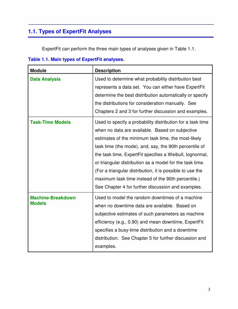
1.1. Types of ExpertFit Analyses
ExpertFit can perform the three main types of analyses given in Table 1.1.
Table 1.1. Main types of ExpertFit analyses.
Module Description
Data Analysis Used to determine what probability distribution best
represents a data set. You can either have ExpertFit
determine the best distribution automatically or specify
the distributions for consideration manually. See
Chapters 2 and 3 for further discussion and examples.
Task-Time Models Used to specify a probability distribution for a task time
when no data are available. Based on subjective
estimates of the minimum task time, the most-likely
task time (the mode), and, say, the 90th percentile of
the task time, ExpertFit specifies a Weibull, lognormal,
or triangular distribution as a model for the task time.
(For a triangular distribution, it is possible to use the
maximum task time instead of the 90th percentile.)
See Chapter 4 for further discussion and examples.
Machine-Breakdown Models
Used to model the random downtimes of a machine
when no downtime data are available. Based on
subjective estimates of such parameters as machine
efficiency (e.g., 0.90) and mean downtime, ExpertFit
specifies a busy-time distribution and a downtime
distribution. See Chapter 5 for further discussion and
examples.
4
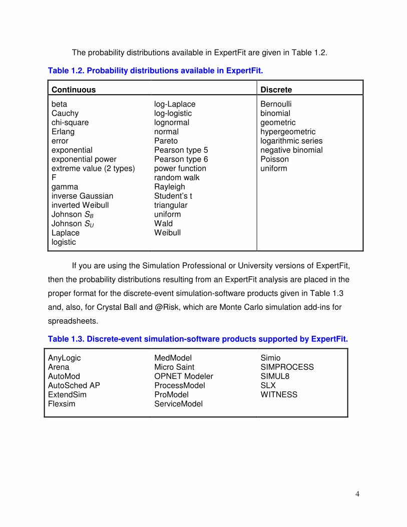
The probability distributions available in ExpertFit are given in Table 1.2.
Table 1.2. Probability distributions available in ExpertFit.
Continuous
Discrete
beta Cauchy chi-square Erlang error exponential exponential power extreme value (2 types) F gamma inverse Gaussian inverted Weibull Johnson SB
Johnson SU Laplace logistic
log-Laplace log-logistic lognormal normal Pareto Pearson type 5 Pearson type 6 power function random walk Rayleigh Student’s t triangular uniform Wald Weibull
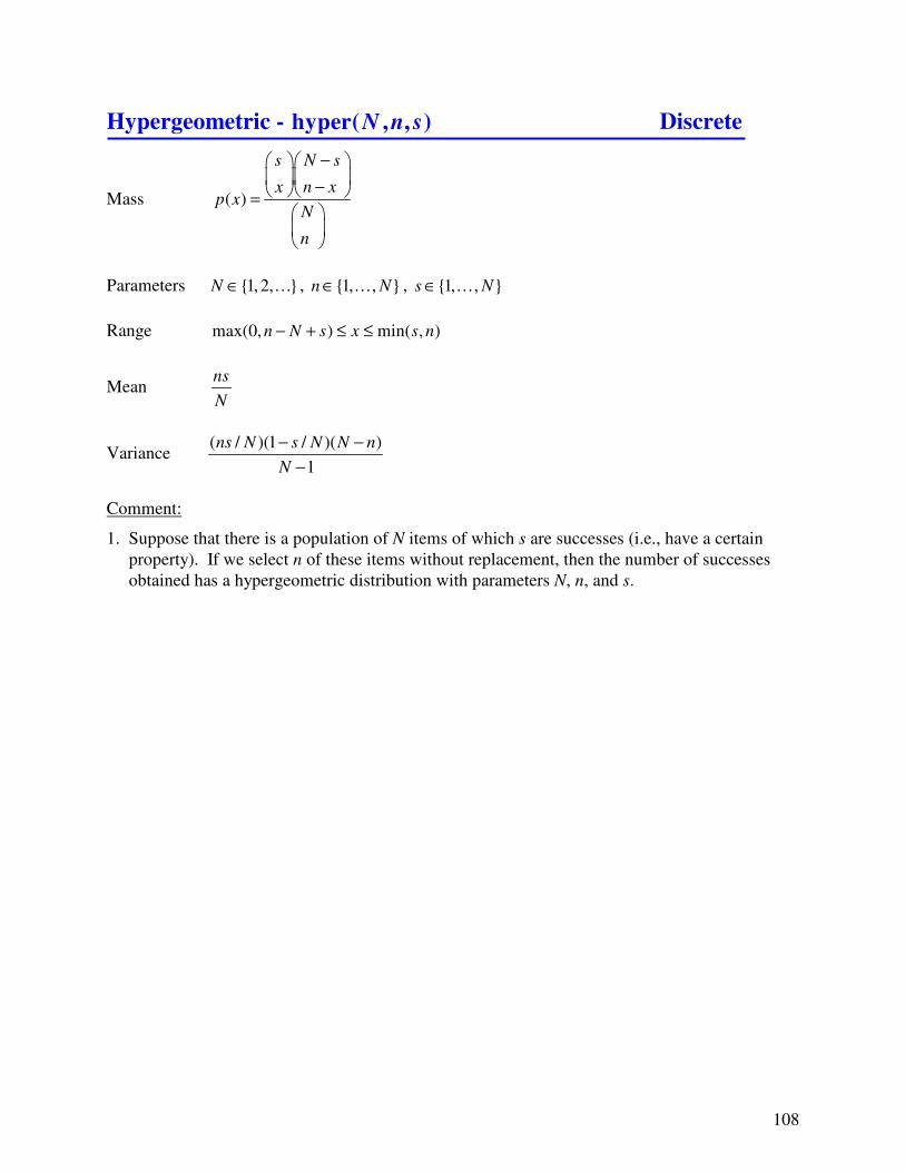
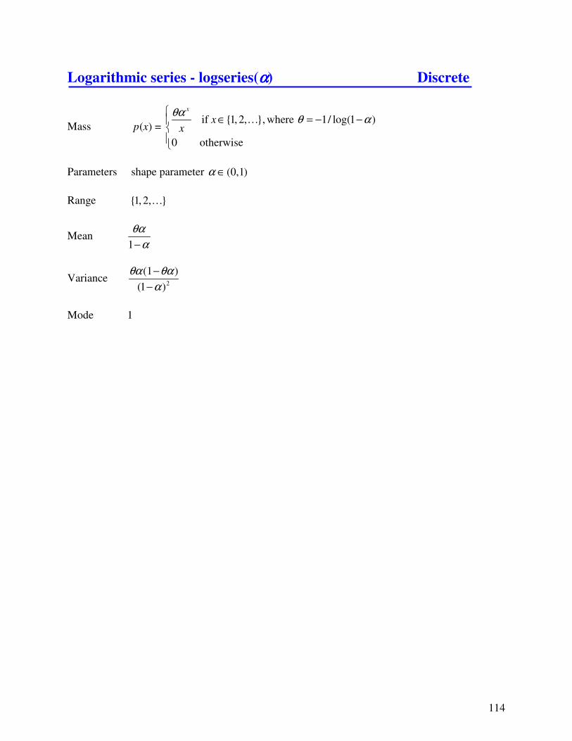
Bernoulli binomial geometric hypergeometric logarithmic series negative binomial Poisson uniform
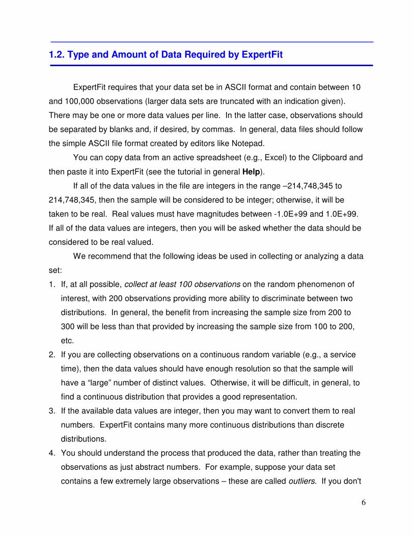
If you are using the Simulation Professional or University versions of ExpertFit,
then the probability distributions resulting from an ExpertFit analysis are placed in the
proper format for the discrete-event simulation-software products given in Table 1.3
and, also, for Crystal Ball and @Risk, which are Monte Carlo simulation add-ins for
spreadsheets.
Table 1.3. Discrete-event simulation-software products supported by ExpertFit.
AnyLogic Arena AutoMod AutoSched AP ExtendSim Flexsim
MedModel Micro Saint OPNET Modeler ProcessModel ProModel ServiceModel
Simio SIMPROCESS SIMUL8 SLX WITNESS
5
If you are using a single-vendor version of ExpertFit, then the resulting probability
distributions are put into the format for that vendor’s software. The Analyst versions of
ExpertFit support Crystal Ball and @RISK.
6
1.2. Type and Amount of Data Required by ExpertFit
ExpertFit requires that your data set be in ASCII format and contain between 10
and 100,000 observations (larger data sets are truncated with an indication given).
There may be one or more data values per line. In the latter case, observations should
be separated by blanks and, if desired, by commas. In general, data files should follow
the simple ASCII file format created by editors like Notepad.
You can copy data from an active spreadsheet (e.g., Excel) to the Clipboard and
then paste it into ExpertFit (see the tutorial in general Help).
If all of the data values in the file are integers in the range –214,748,345 to
214,748,345, then the sample will be considered to be integer; otherwise, it will be
taken to be real. Real values must have magnitudes between -1.0E+99 and 1.0E+99.
If all of the data values are integers, then you will be asked whether the data should be
considered to be real valued.
We recommend that the following ideas be used in collecting or analyzing a data
set:
1. If, at all possible, collect at least 100 observations on the random phenomenon of
interest, with 200 observations providing more ability to discriminate between two
distributions. In general, the benefit from increasing the sample size from 200 to
300 will be less than that provided by increasing the sample size from 100 to 200,
etc.
2. If you are collecting observations on a continuous random variable (e.g., a service
time), then the data values should have enough resolution so that the sample will
have a “large” number of distinct values. Otherwise, it will be difficult, in general, to
find a continuous distribution that provides a good representation.
3. If the available data values are integer, then you may want to convert them to real
numbers. ExpertFit contains many more continuous distributions than discrete
distributions.
4. You should understand the process that produced the data, rather than treating the
observations as just abstract numbers. For example, suppose your data set
contains a few extremely large observations – these are called outliers. If you don't
7
understand the problem context, then it will be difficult to know whether these large
observations are really legitimate or, perhaps, the result of measuring or recording
errors.
5. If you have collected times of arrival of “customers,” then these can be converted to
interarrival times using the ExpertFit transformation “DIFF.”
8
1.3. Installation Instructions
ExpertFit is shipped on a CD and the security key (dongle) must be attached to
your computer to run the software. To install ExpertFit, insert the enclosed CD into the
corresponding drive. The Setup program should start within a few seconds. If not use
START, RUN to invoke SETUP.EXE on the CD. When the Setup program finishes, a
Windows program group will be created to hold an icon for ExpertFit and for reading a
README.WRI file. (This file contains any available notifications and also clarifications
for this User’s Guide.) Click on the icon to start ExpertFit.
ExpertFit saves information on the user organization in the security key. If this
information has not been set before the software was shipped to you, then on the first
execution you will be prompted for a permanent user name.
9
1.4. ExpertFit Help System
There are two main types of help available in ExpertFit: context-dependent and
general. Context-dependent help is available for every options and results screen, and
is accessed by clicking on the displayed Help button.
General help is accessed by clicking on the Help pull-down menu in the Menu
Bar at the top of the screen. This menu contains the following entries:
• Contents
• Context-Dependent
• Glossary
• Search
• Tutorials
• User’s Guide
• About ExpertFit
The Contents entry includes the following categories:
• Introduction to ExpertFit
• Types of ExpertFit Analyses
• Standard Mode Versus Advanced Mode
• Normal Precision Versus High Precision
• ExpertFit Software Architecture
• Tutorials
• Glossary
• Additional Documentation
• Customer Support
10
1.5. ExpertFit Software Architecture
ExpertFit uses the concept of a Project, which is a file containing one or more
analysis items. In the case of a simulation study, a Project could contain several items
corresponding to different data sets and their corresponding ExpertFit analyses, and
other items corresponding to Task-Time Models or Machine-Breakdown Models. A
Project allows you to save the results of an ExpertFit analysis for future reuse.
When an ExpertFit Project is created or read from a file, a Project Window is
created to represent it. This window acts as a directory for the analysis items contained
in the Project. Buttons at the bottom of the window allow you to create new elements,
to change an element’s name or description, to begin a new (or return to an existing)
analysis, and to delete an element.
11
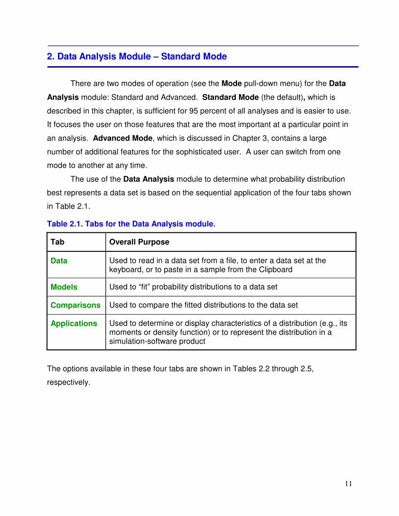
2. Data Analysis Module – Standard Mode
There are two modes of operation (see the Mode pull-down menu) for the Data
Analysis module: Standard and Advanced. Standard Mode (the default), which is
described in this chapter, is sufficient for 95 percent of all analyses and is easier to use.
It focuses the user on those features that are the most important at a particular point in
an analysis. Advanced Mode, which is discussed in Chapter 3, contains a large
number of additional features for the sophisticated user. A user can switch from one
mode to another at any time.
The use of the Data Analysis module to determine what probability distribution
best represents a data set is based on the sequential application of the four tabs shown
in Table 2.1.
Table 2.1. Tabs for the Data Analysis module.
Tab Overall Purpose
Data Used to read in a data set from a file, to enter a data set at the keyboard, or to paste in a sample from the Clipboard
Models Used to “fit” probability distributions to a data set
Comparisons Used to compare the fitted distributions to the data set
Applications Used to determine or display characteristics of a distribution (e.g., its moments or density function) or to represent the distribution in a simulation-software product
The options available in these four tabs are shown in Tables 2.2 through 2.5,
respectively.
12
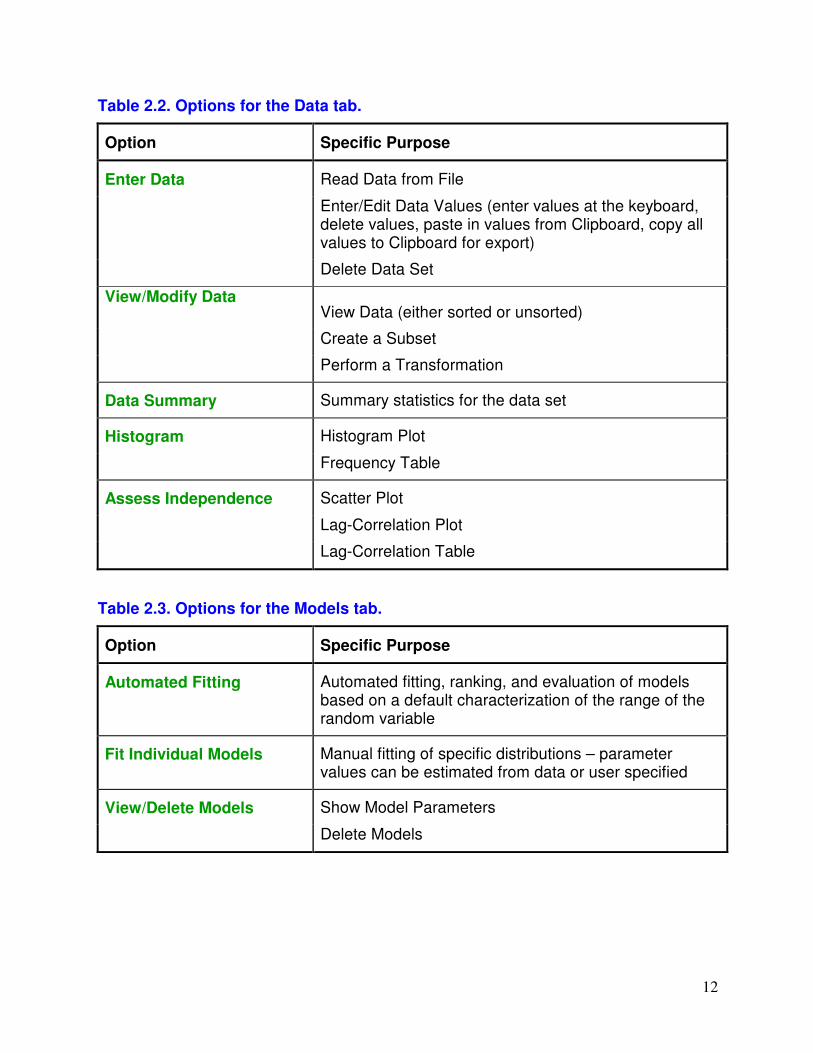
Table 2.2. Options for the Data tab.
Option Specific Purpose
Enter Data Read Data from File
Enter/Edit Data Values (enter values at the keyboard, delete values, paste in values from Clipboard, copy all values to Clipboard for export)
Delete Data Set
View/Modify Data View Data (either sorted or unsorted)
Create a Subset
Perform a Transformation
Data Summary Summary statistics for the data set
Histogram Histogram Plot
Frequency Table
Assess Independence Scatter Plot
Lag-Correlation Plot
Lag-Correlation Table
Table 2.3. Options for the Models tab.
Option Specific Purpose
Automated Fitting
Automated fitting, ranking, and evaluation of models based on a default characterization of the range of the random variable
Fit Individual Models Manual fitting of specific distributions – parameter values can be estimated from data or user specified
View/Delete Models Show Model Parameters
Delete Models
13
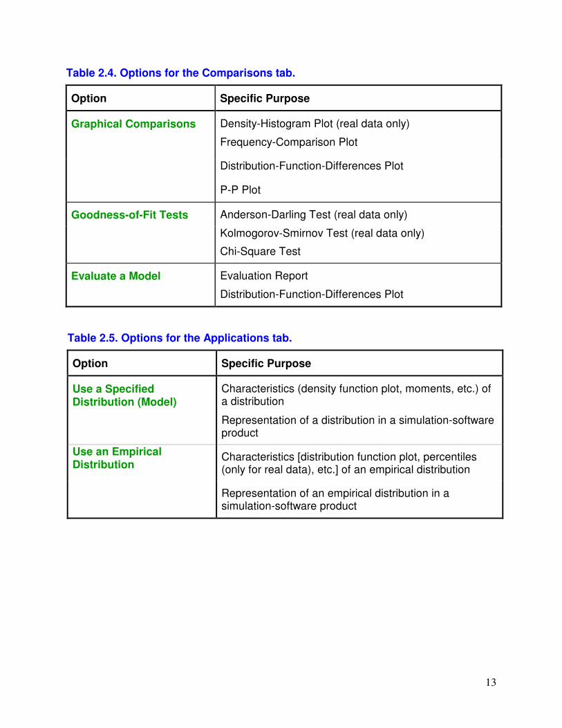
Table 2.4. Options for the Comparisons tab.
Option Specific Purpose
Graphical Comparisons Density-Histogram Plot (real data only)
Frequency-Comparison Plot
Distribution-Function-Differences Plot
P-P Plot
Goodness-of-Fit Tests Anderson-Darling Test (real data only)
Kolmogorov-Smirnov Test (real data only)
Chi-Square Test
Evaluate a Model Evaluation Report
Distribution-Function-Differences Plot
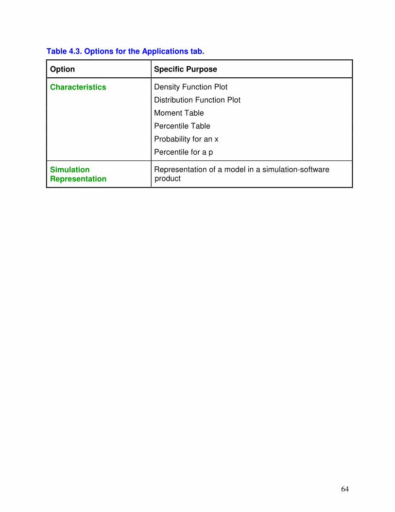
Table 2.5. Options for the Applications tab.
Option Specific Purpose
Use a Specified Distribution (Model)
Characteristics (density function plot, moments, etc.) of a distribution
Representation of a distribution in a simulation-software product
Use an Empirical Distribution
Characteristics [distribution function plot, percentiles (only for real data), etc.] of an empirical distribution
Representation of an empirical distribution in a simulation-software product
14
Although there are different ways that these four tabs could be used to
determine the best distribution for a data set, the following are the explicit steps that we
recommend for real data (see Example 2.4 for integer data):
1. Obtain a data set using the Data tab – see Section 1.2 for a discussion of the type
and amount of data required.
2. View the resulting Data-Summary Table (at the Data tab) – provides information on
the center, shape, and range of the true density (mass) function.
3. Make a histogram of your data (used in Step 5) using the Data tab – see the
Constructing a Histogram from Your Data tutorial in the online help.
4. Select the distribution that is the best representation for your data using the
Automated Fitting option at the Models tab.
5. Confirm using the Comparisons tab that the best distribution as determined by
ExpertFit is, in fact, satisfactory in an absolute sense – See Section 2.1 for
recommendations.
6. If you are doing simulation modeling, then either represent the best-fitting
distribution (if good in an absolute sense) or an empirical distribution based on your
data (if the best distribution is not satisfactory) in your simulation software using the
Applications tab.
Four examples of the use of the Data Analysis module are given in Section 2.2.
15
2.1. Confirmation of the Best Distribution
Before actually using the best model, we recommend that some amount of
confirmation of this model be done using the options in the Comparisons tab. We
suggest that a Density-Histogram Plot and/or a Frequency-Comparison Plot be
made with an appropriately constructed histogram. When the maximum of the density
function of the best model is “far” from x = 0, then the former plot is probably preferable.
If, on the other hand, the maximum occurs “close” to x = 0, then the latter plot will often
be more useful. This is because it may be difficult in this case to determine from a
histogram whether the true underlying density function strictly decreases as x increases
(similar to an exponential density) or whether the density function has its mode (x-value
where the maximum occurs) close to x = 0 (similar to a lognormal density with shape
parameter = 3/2). Care must be taken when using these plots since the choice of the
histogram intervals is somewhat subjective.
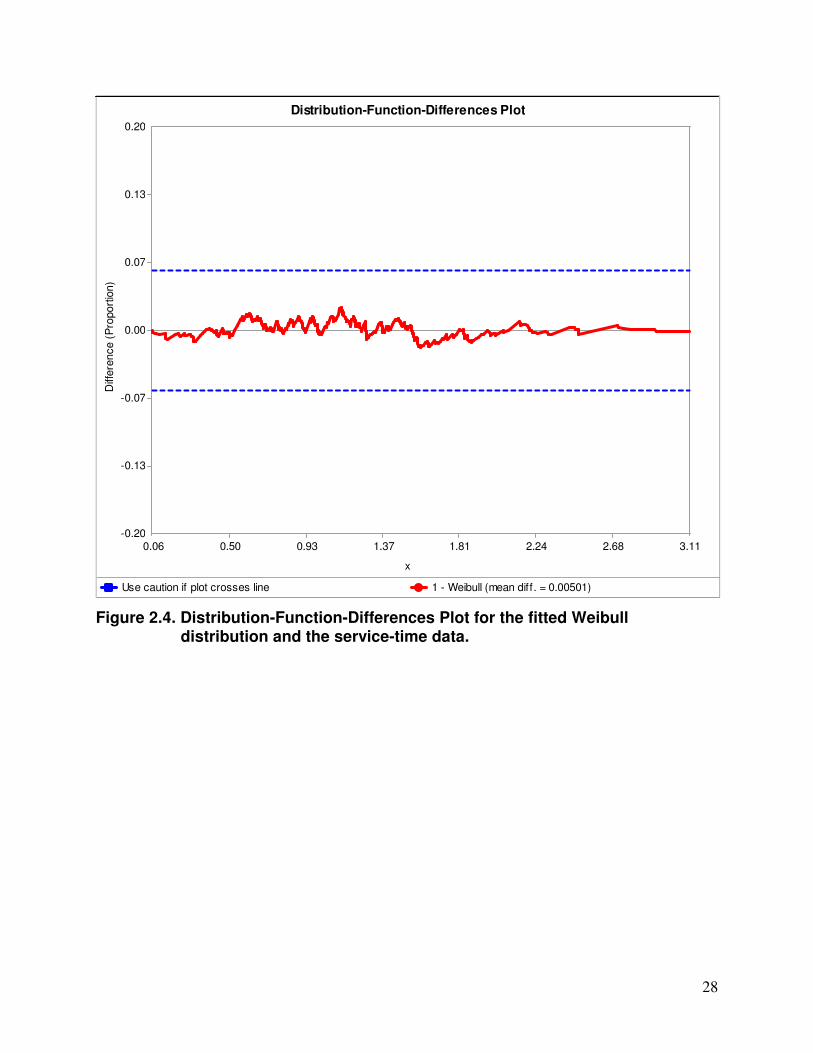
We also recommend that a Distribution-Function-Differences Plot and a
P-P Plot be used to confirm the quality of the best model.
Finally, one might perform the Anderson-Darling Test, the Kolmogorov-
Smirnov Test, and/or the Chi-Square Test in order to get a formal evaluation of the
best-fitting model.
16
2.2. Examples
We now present four examples of the use of the Data Analysis module,
following the six-step approach outlined at the beginning of this chapter. For the first
example, we give the ExpertFit commands necessary to accomplish a particular part of
the analysis and then the actual results of the analysis. For the other examples, we
only discuss the results.
Examples 2.1 through 2.3 use High Precision (the default) – see the “Overview”
in the Precision pull-down menu. It doesn’t matter which option you use for the integer
data of Example 2.4, since the two options are identical in this case.
17
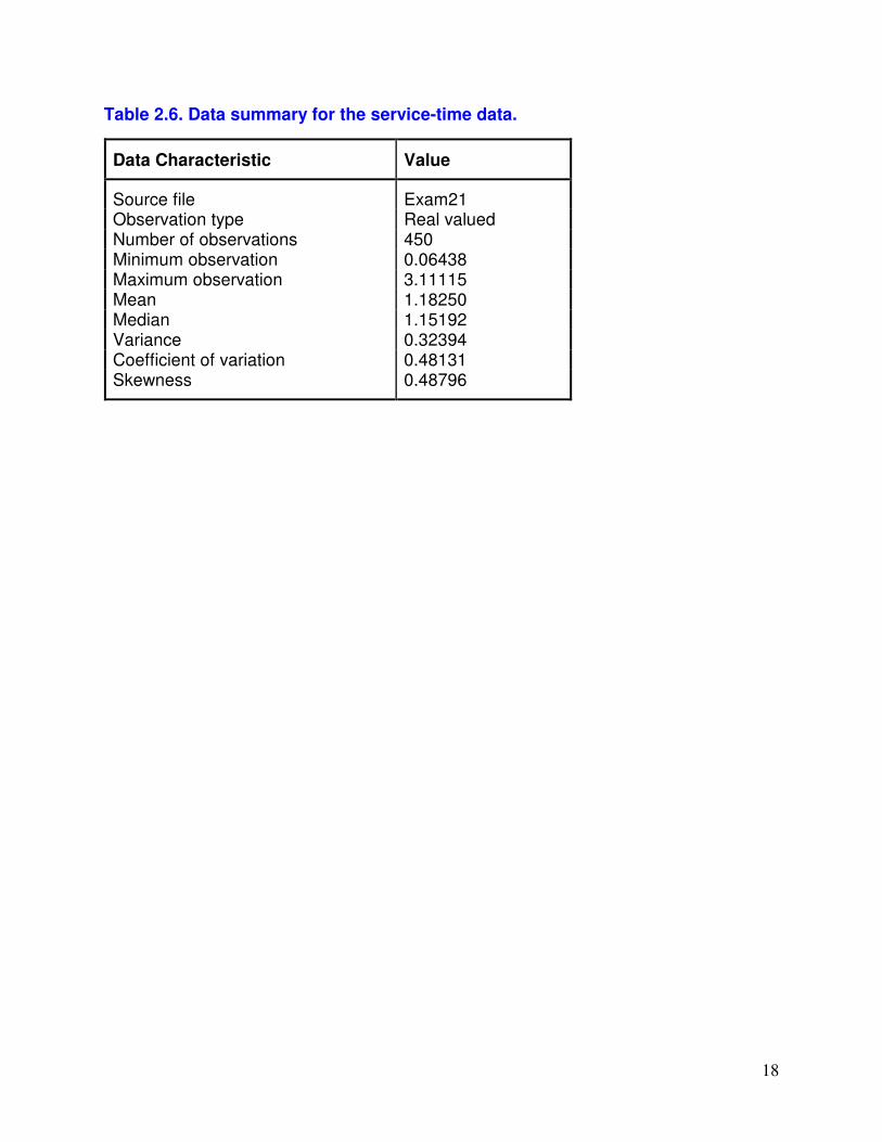
Example 2.1: Customer Service Times
A: The Data-Summary Table for this set of n = 450 service times (read in the Data
tab) is given in Table 2.6. The positive value of the sample skewness indicates that the
underlying distribution of the data is skewed to the right (i.e., it has a longer right tail
than left tail). This is supported by the sample mean being larger than the sample
median.
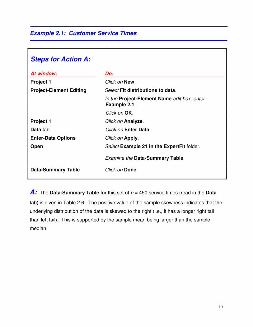
Steps for Action A: At window: Do:
Project 1 Click on New.
Project-Element Editing Select Fit distributions to data.
In the Project-Element Name edit box, enter Example 2.1.
Click on OK.
Project 1 Click on Analyze.
Data tab Click on Enter Data.
Enter-Data Options Click on Apply.
Open Select Example 21 in the ExpertFit folder. Examine the Data-Summary Table. Data-Summary Table Click on Done.
18
Table 2.6. Data summary for the service-time data.
Data Characteristic Value
Source file Exam21 Observation type Real valued Number of observations 450 Minimum observation 0.06438 Maximum observation 3.11115 Mean 1.18250 Median 1.15192 Variance 0.32394 Coefficient of variation 0.48131 Skewness 0.48796
19
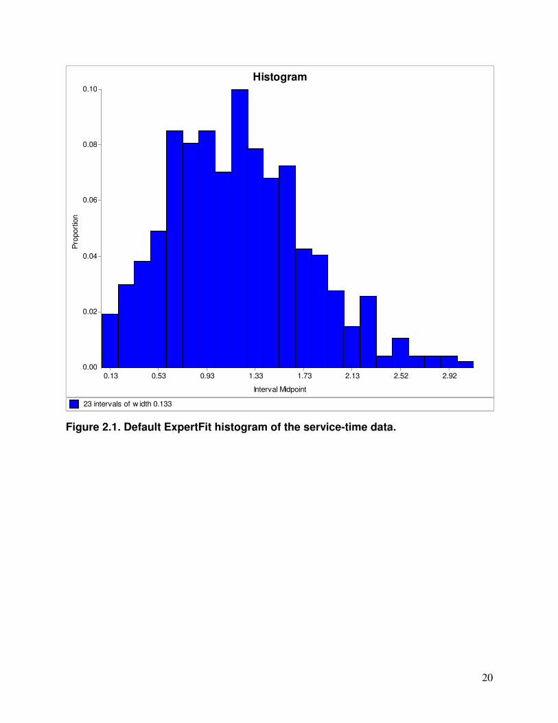
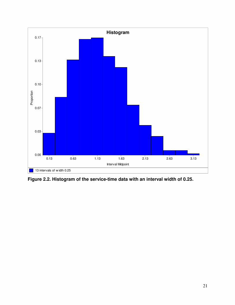
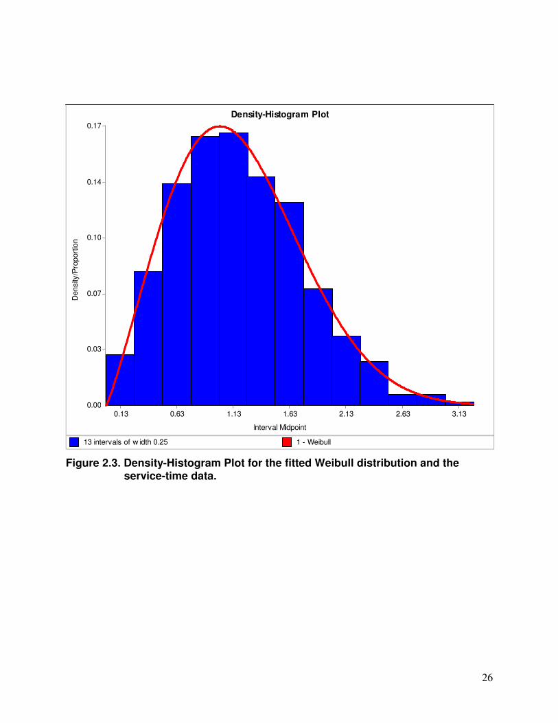
B: In Figure 2.1 we present the default ExpertFit histogram for the service-time data.
Note that the histogram is quite “ragged,” since the interval width is too small. Using a
trial-and-error approach discussed in the Constructing a Histogram from Your Data
tutorial, we determined that a better histogram is obtained by using an interval width of
0.25. The improved “smooth” histogram is shown in Figure 2.2. In general we
recommend that you construct your own histogram rather than rely on the ExpertFit
default. There is no definitive prescription for choosing histogram intervals!
Note that the histogram interval width can also be changed by using the
two buttons with arrowheads at the top of the histogram screen. The left (right)
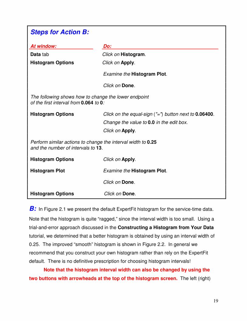
Steps for Action B: At window: Do:
Data tab Click on Histogram.
Histogram Options Click on Apply. Examine the Histogram Plot. Click on Done.
The following shows how to change the lower endpoint of the first interval from 0.064 to 0: Histogram Options Click on the equal-sign ("=") button next to 0.06400.
Change the value to 0.0 in the edit box.
Click on Apply.
Perform similar actions to change the interval width to 0.25 and the number of intervals to 13. Histogram Options Click on Apply. Histogram Plot Examine the Histogram Plot. Click on Done. Histogram Options Click on Done.
20
23 intervals of w idth 0.133
0.00
0.02
0.04
0.06
0.08
0.10
0.13 0.53 0.93 1.33 1.73 2.13 2.52 2.92
Pro
port
ion
HistogramHistogram
Interval Midpoint
Figure 2.1. Default ExpertFit histogram of the service-time data.
21
13 intervals of w idth 0.25
0.00
0.03
0.07
0.10
0.13
0.17
0.13 0.63 1.13 1.63 2.13 2.63 3.13
Pro
port
ion
HistogramHistogram
Interval Midpoint
Figure 2.2. Histogram of the service-time data with an interval width of 0.25.
22
button decreases (increases) the interval width by 5 percent, and can be applied
repeatedly.
23
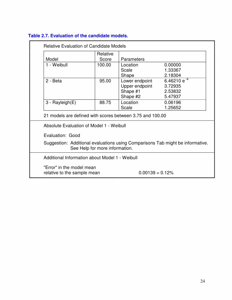
C: We begin the actual process of finding a distribution that is a good representation
for our data by selecting the Automated Fitting option at the Models tab. Based on
certain heuristics, ExpertFit determined that the “best” representation for the data is
provided by a Weibull distribution (see Table 2.7) with location, scale, and shape
parameters of 0, 1.334, and 2.183, respectively. This best model received a Relative
Score of 100.00 and its Absolute Evaluation message is “Good,” indicating no reason
for concern. (See the context-dependent online help for a discussion of the terms in
boldface.) Furthermore, the model mean and the sample mean are almost identical.
Note that the third-best fitting model is a Rayleigh distribution with an estimated
location parameter (denoted by “E”) of 0.062. (If we were to click on View/Delete
Models at the Models tab, we would see that the normal distribution was not
automatically fit to our non-negative service-time data. This is because the normal
distribution can take on negative values. However, the normal distribution could, if
desired, be fit to our data using the Fit Individual Models option at the Models tab.)
Steps for Action C: At window: Do:
Data tab Click on the Models tab.
Models tab Click on Automated Fitting. Examine Automated-Fitting Results. Automated-Fitting Results Click on Done.
This sample of n = 856 observations corresponds to loading times (in hours) for
an oil tanker. The Data-Summary Table is given in Table 2.9; the positive skewness
and the fact that the mean is larger than the median both suggest the underlying
distribution of the data has a longer right tail than left tail.
A histogram of the data with a lower endpoint of 0, an interval width of 0.1, and
23 intervals is given in Figure 2.5 – the latter two choices were obtained by trial and
error. Note that the histogram is reasonably smooth, skewed to the right, and is
definitely shifted away from the origin.
The process of finding a distribution that is a good representation for the data
once again begins by selecting Automated Fitting. The log-logistic distribution was
found by ExpertFit to provide the best representation (see Table 2.10), with a Relative
Score of 100.00. The Absolute Evaluation for the log-logistic distribution is “Good,”
which indicates that there is no reason for concern. Also, the model mean and sample
mean differ by only 0.34 percent.
Table 2.9. Data summary for the ship-loading times.
Data Characteristic Value
Source file Exam22 Observation type Real valued Number of observations 856 Minimum observation 0.36736 Maximum observation 2.17986 Mean 0.84244 Median 0.82326 Variance 0.03584 Coefficient of variation 0.22471 Skewness 1.82628
33
23 intervals of w idth 0.1
0.00
0.05
0.10
0.15
0.20
0.25
0.05 0.35 0.65 0.95 1.25 1.55 1.85 2.15
Pro
port
ion
HistogramHistogram
Interval Midpoint
Figure 2.5. Histogram of the ship-loading times.
34
Table 2.10. Evaluation of the candidate models.
Relative Evaluation of Candidate Models
Relative
Model Score Parameters
1 – Log-Logistic 100.00 Location Scale Shape
0.00000 0.82199 8.84087
2 – Pearson Type VI 91.35 Location Scale Shape #1 Shape #2
0.00000 0.25314 99.97455 31.06366
3 – Pearson Type V 88.46 Location Scale Shape
0.00000 19.18409 23.78474
27 models are defined with scores between 1.92 and 100.00
Absolute Evaluation of Model 1 – Log-Logistic
Evaluation: Good
Suggestion: Additional evaluations using Comparisons Tab might be informative.
See Help for more information.
Additional Information about Model 1 – Log-Logistic
"Error" in the model mean
relative to the sample mean 0.00290 = 0.34%
35
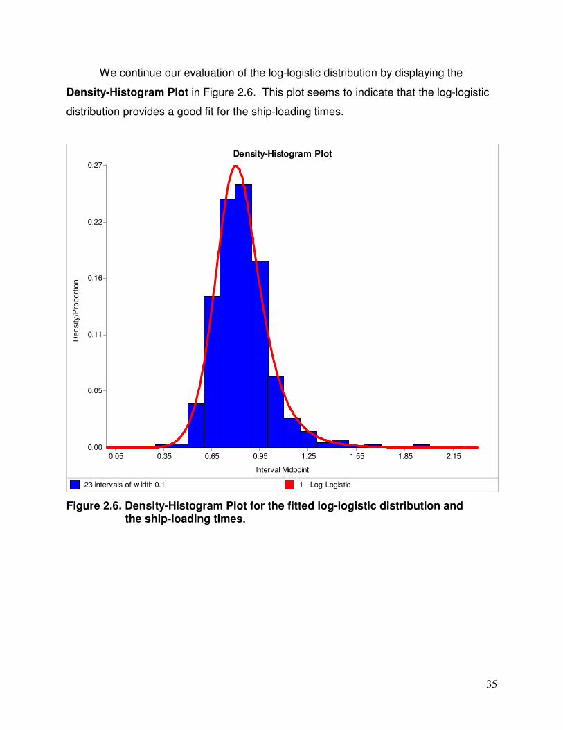
We continue our evaluation of the log-logistic distribution by displaying the
Density-Histogram Plot in Figure 2.6. This plot seems to indicate that the log-logistic
distribution provides a good fit for the ship-loading times.
23 intervals of w idth 0.1 1 - Log-Logistic
0.00
0.05
0.11
0.16
0.22
0.27
0.05 0.35 0.65 0.95 1.25 1.55 1.85 2.15
Density
/Pro
port
ion
Density-Histogram PlotDensity-Histogram Plot
Interval Midpoint
Figure 2.6. Density-Histogram Plot for the fitted log-logistic distribution and the ship-loading times.
36
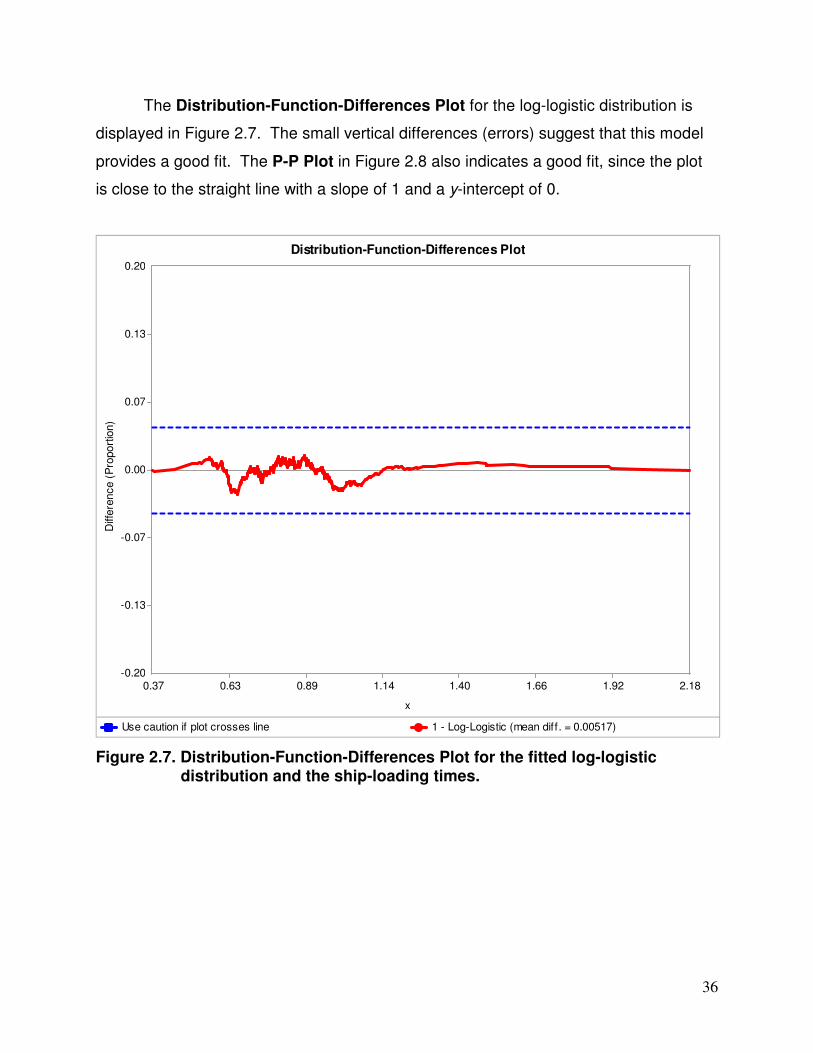
The Distribution-Function-Differences Plot for the log-logistic distribution is
displayed in Figure 2.7. The small vertical differences (errors) suggest that this model
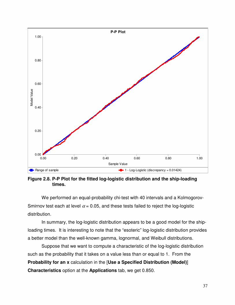
provides a good fit. The P-P Plot in Figure 2.8 also indicates a good fit, since the plot
is close to the straight line with a slope of 1 and a y-intercept of 0.
Use caution if plot crosses line 1 - Log-Logistic (mean diff. = 0.00517)
Figure 2.7. Distribution-Function-Differences Plot for the fitted log-logistic distribution and the ship-loading times.
37
Range of sample 1 - Log-Logistic (discrepancy = 0.01424)
0.00
0.20
0.40
0.60
0.80
1.00
0.00 0.20 0.40 0.60 0.80 1.00
Model V
alu
eP-P PlotP-P Plot
Sample Value
Figure 2.8. P-P Plot for the fitted log-logistic distribution and the ship-loading times.
We performed an equal-probability chi-test with 40 intervals and a Kolmogorov-
Smirnov test each at level α = 0.05, and these tests failed to reject the log-logistic
distribution.
In summary, the log-logistic distribution appears to be a good model for the ship-
loading times. It is interesting to note that the “esoteric” log-logistic distribution provides
a better model than the well-known gamma, lognormal, and Weibull distributions.
Suppose that we want to compute a characteristic of the log-logistic distribution
such as the probability that it takes on a value less than or equal to 1. From the
Probability for an x calculation in the [Use a Specified Distribution (Model)]
Characteristics option at the Applications tab, we get 0.850.
38
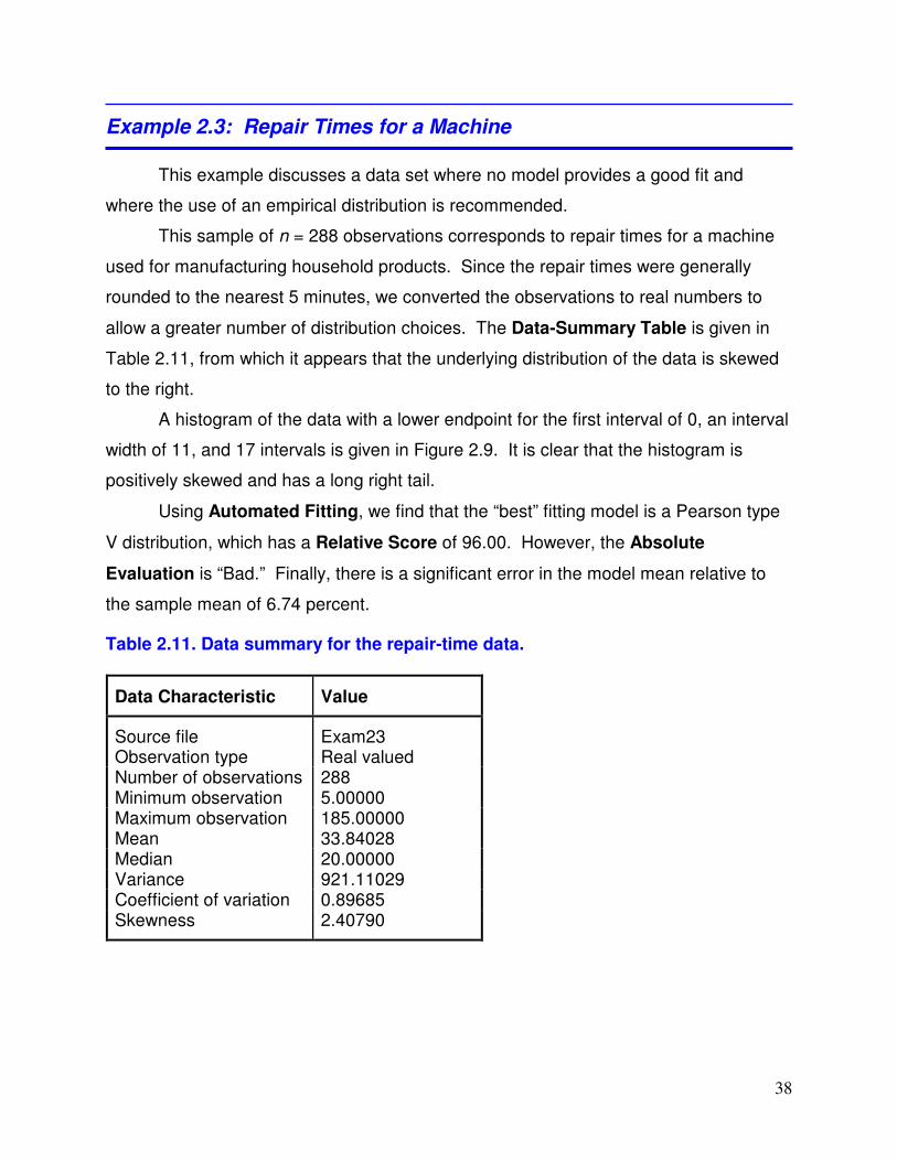
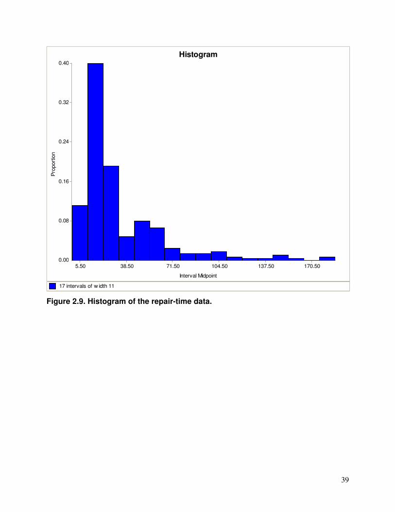
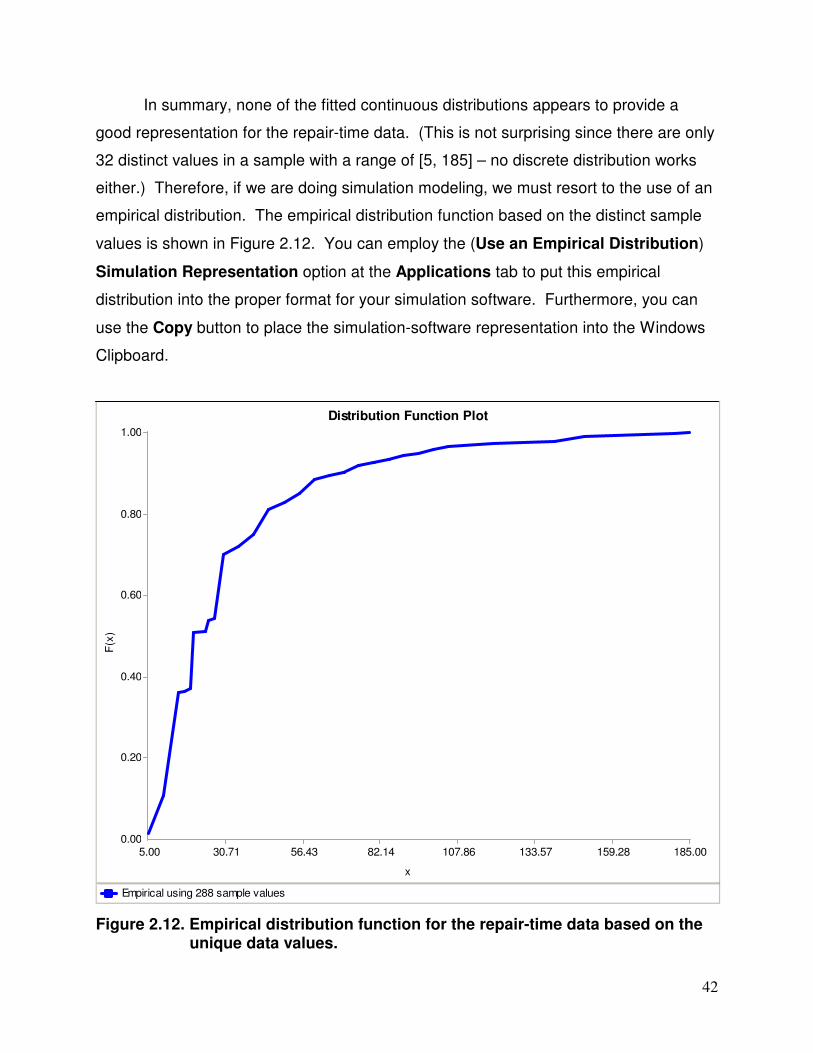
Example 2.3: Repair Times for a Machine
This example discusses a data set where no model provides a good fit and
where the use of an empirical distribution is recommended.
This sample of n = 288 observations corresponds to repair times for a machine
used for manufacturing household products. Since the repair times were generally
rounded to the nearest 5 minutes, we converted the observations to real numbers to
allow a greater number of distribution choices. The Data-Summary Table is given in
Table 2.11, from which it appears that the underlying distribution of the data is skewed
to the right.
A histogram of the data with a lower endpoint for the first interval of 0, an interval
width of 11, and 17 intervals is given in Figure 2.9. It is clear that the histogram is
positively skewed and has a long right tail.
Using Automated Fitting, we find that the “best” fitting model is a Pearson type
V distribution, which has a Relative Score of 96.00. However, the Absolute
Evaluation is “Bad.” Finally, there is a significant error in the model mean relative to
the sample mean of 6.74 percent.
Table 2.11. Data summary for the repair-time data.
Data Characteristic Value
Source file Exam23 Observation type Real valued Number of observations 288 Minimum observation 5.00000 Maximum observation 185.00000 Mean 33.84028 Median 20.00000 Variance 921.11029 Coefficient of variation 0.89685 Skewness 2.40790
39
17 intervals of w idth 11
0.00
0.08
0.16
0.24
0.32
0.40
5.50 38.50 71.50 104.50 137.50 170.50
Pro
port
ion
HistogramHistogram
Interval Midpoint
Figure 2.9. Histogram of the repair-time data.
40
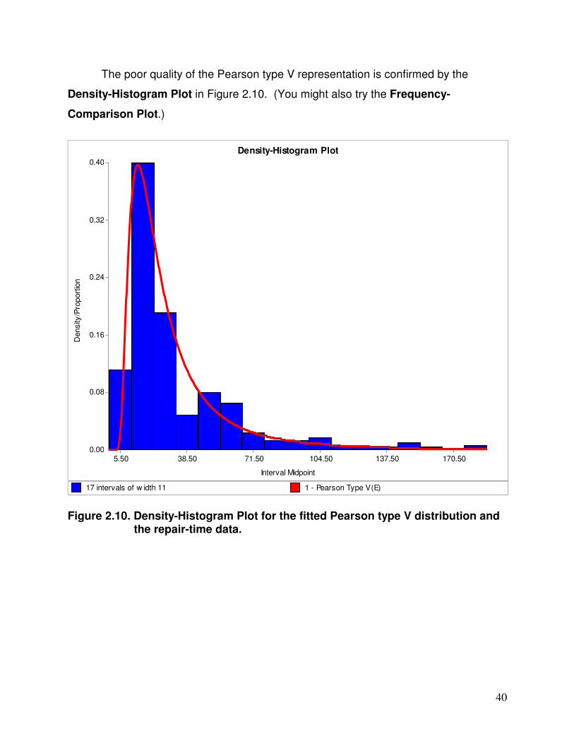
The poor quality of the Pearson type V representation is confirmed by the
Density-Histogram Plot in Figure 2.10. (You might also try the Frequency-
Comparison Plot.)
17 intervals of w idth 11 1 - Pearson Type V(E)
0.00
0.08
0.16
0.24
0.32
0.40
5.50 38.50 71.50 104.50 137.50 170.50
Density
/Pro
port
ion
Density-Histogram PlotDensity-Histogram Plot
Interval Midpoint
Figure 2.10. Density-Histogram Plot for the fitted Pearson type V distribution and the repair-time data.
41
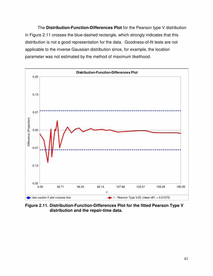
The Distribution-Function-Differences Plot for the Pearson type V distribution
in Figure 2.11 crosses the blue-dashed rectangle, which strongly indicates that this
distribution is not a good representation for the data. Goodness-of-fit tests are not
applicable to the inverse Gaussian distribution since, for example, the location
parameter was not estimated by the method of maximum likelihood.
Use caution if plot crosses line 1 - Pearson Type V(E) (mean diff. = 0.01272)
Distribution Function PlotDistribution Function Plot
x
Figure 2.12. Empirical distribution function for the repair-time data based on the unique data values.
43
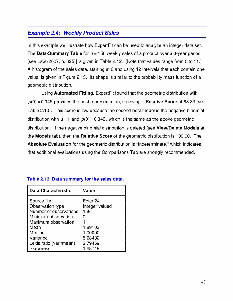
Example 2.4: Weekly Product Sales
In this example we illustrate how ExpertFit can be used to analyze an integer data set.
The Data-Summary Table for n = 156 weekly sales of a product over a 3-year period
[see Law (2007, p. 325)] is given in Table 2.12. (Note that values range from 0 to 11.)
A histogram of the sales data, starting at 0 and using 12 intervals that each contain one
value, is given in Figure 2.13. Its shape is similar to the probability mass function of a
geometric distribution.
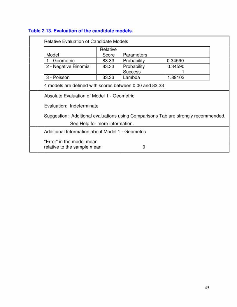
Using Automated Fitting, ExpertFit found that the geometric distribution with
ˆ( ) .=0 0 346p provides the best representation, receiving a Relative Score of 83.33 (see
Table 2.13). This score is low because the second-best model is the negative binomial
distribution with ˆ = 1s and ˆ( ) .=0 0 346p , which is the same as the above geometric
distribution. If the negative binomial distribution is deleted (see View/Delete Models at
the Models tab), then the Relative Score of the geometric distribution is 100.00. The
Absolute Evaluation for the geometric distribution is “Indeterminate,” which indicates
that additional evaluations using the Comparisons Tab are strongly recommended.
Data Characteristic Value
Source file Exam24 Observation type Integer valued Number of observations 156 Minimum observation 0 Maximum observation 11 Mean 1.89103 Median 1.00000 Variance 5.28482 Lexis ratio (var./mean) 2.79469 Skewness 1.68749
Table 2.12. Data summary for the sales data.
44
12 intervals of w idth 1
0.00
0.08
0.15
0.23
0.30
0.38
0 2 4 6 8 10
Pro
port
ion
HistogramHistogram
Value
Figure 2.13. Histogram of the sales data.
45
Table 2.13. Evaluation of the candidate models.
Relative Evaluation of Candidate Models
Relative
Model Score Parameters
1 - Geometric 83.33 Probability 0.34590
2 - Negative Binomial 83.33 Probability Success
0.34590 1
3 - Poisson 33.33 Lambda 1.89103
4 models are defined with scores between 0.00 and 83.33
Absolute Evaluation of Model 1 - Geometric
Evaluation: Indeterminate
Suggestion: Additional evaluations using Comparisons Tab are strongly recommended.
See Help for more information.
Additional Information about Model 1 - Geometric
""Error" in the model mean
relative to the sample mean 0
46
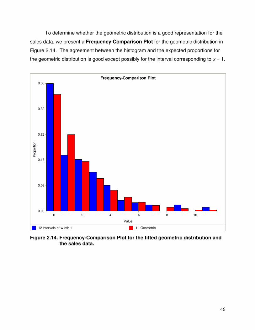
To determine whether the geometric distribution is a good representation for the
sales data, we present a Frequency-Comparison Plot for the geometric distribution in
Figure 2.14. The agreement between the histogram and the expected proportions for
the geometric distribution is good except possibly for the interval corresponding to x = 1.
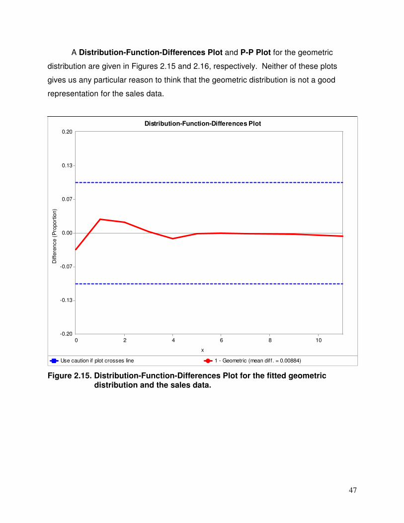
Figure 2.15. Distribution-Function-Differences Plot for the fitted geometric distribution and the sales data.
48
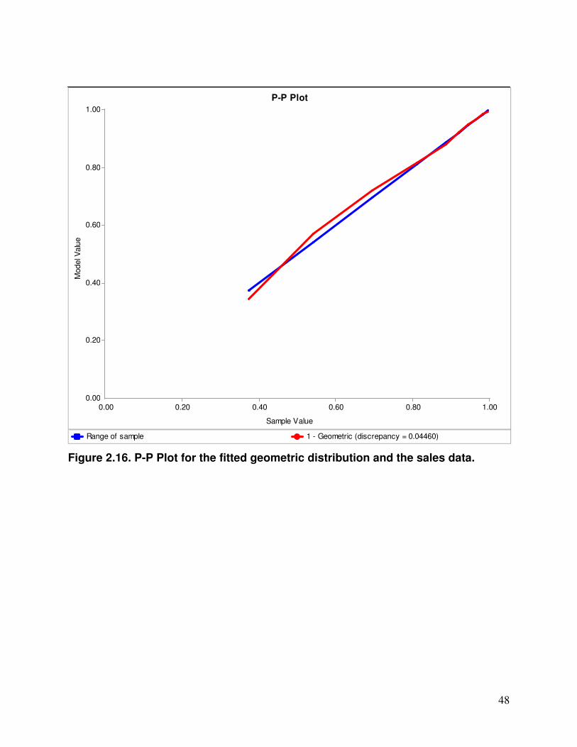
Range of sample 1 - Geometric (discrepancy = 0.04460)
0.00
0.20
0.40
0.60
0.80
1.00
0.00 0.20 0.40 0.60 0.80 1.00
Model V
alu
e
P-P PlotP-P Plot
Sample Value
Figure 2.16. P-P Plot for the fitted geometric distribution and the sales data.
49
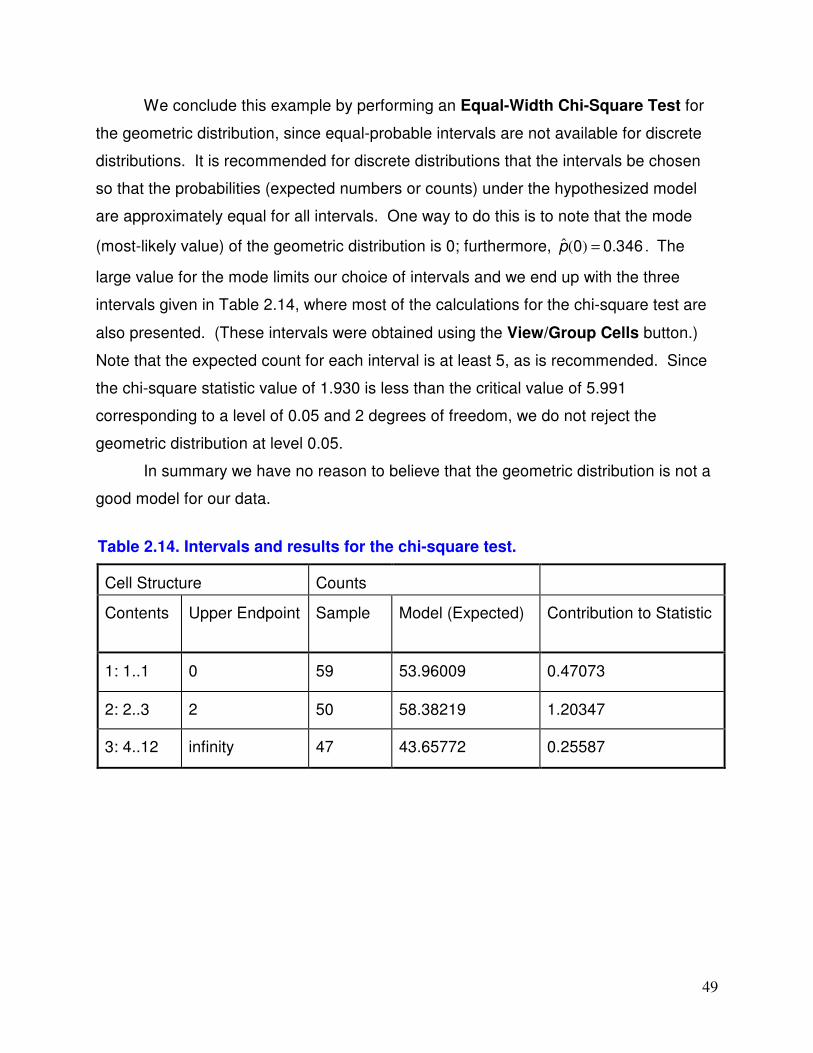
We conclude this example by performing an Equal-Width Chi-Square Test for
the geometric distribution, since equal-probable intervals are not available for discrete
distributions. It is recommended for discrete distributions that the intervals be chosen
so that the probabilities (expected numbers or counts) under the hypothesized model
are approximately equal for all intervals. One way to do this is to note that the mode
(most-likely value) of the geometric distribution is 0; furthermore, ˆ( ) .=0 0 346p . The
large value for the mode limits our choice of intervals and we end up with the three
intervals given in Table 2.14, where most of the calculations for the chi-square test are
also presented. (These intervals were obtained using the View/Group Cells button.)
Note that the expected count for each interval is at least 5, as is recommended. Since
the chi-square statistic value of 1.930 is less than the critical value of 5.991
corresponding to a level of 0.05 and 2 degrees of freedom, we do not reject the
geometric distribution at level 0.05.
In summary we have no reason to believe that the geometric distribution is not a
good model for our data.
Table 2.14. Intervals and results for the chi-square test.
Cell Structure Counts
Contents Upper Endpoint Sample Model (Expected) Contribution to Statistic
1: 1..1 0 59 53.96009 0.47073
2: 2..3 2 50 58.38219 1.20347
3: 4..12 infinity 47 43.65772 0.25587
50
3. Data Analysis Module – Advanced Mode
In this chapter we discuss Advanced Mode for the Data Analysis module,
which is accessed from the Mode pull-down menu at the top of the screen. Advanced
Mode contains a large number of features that are not in Standard Mode – these
features will be of interest to the sophisticated user. However, a user can switch from
one mode to another at any time.
The use of Advanced Mode for the Data Analysis module to determine what
probability distribution best represents a data set is based on the sequential application
of the four tabs shown in Table 3.1. (These tabs are similar to those in Table 2.1.)
Table 3.1. Tabs for the Data Analysis module.
Tab Overall Purpose
Data Used to read in a data set from a file, enter a data set at the keyboard, or paste in a sample from the Clipboard
Models Used to “fit” probability distributions to a data set
Comparisons Used to compare the fitted distributions to the data set
Applications Used to determine or display characteristics of a distribution (e.g., its moments or density function) or to represent the distribution in a simulation-software product
The options available in these four tabs are shown in Tables 3.2 through 3.5, respectively.
51
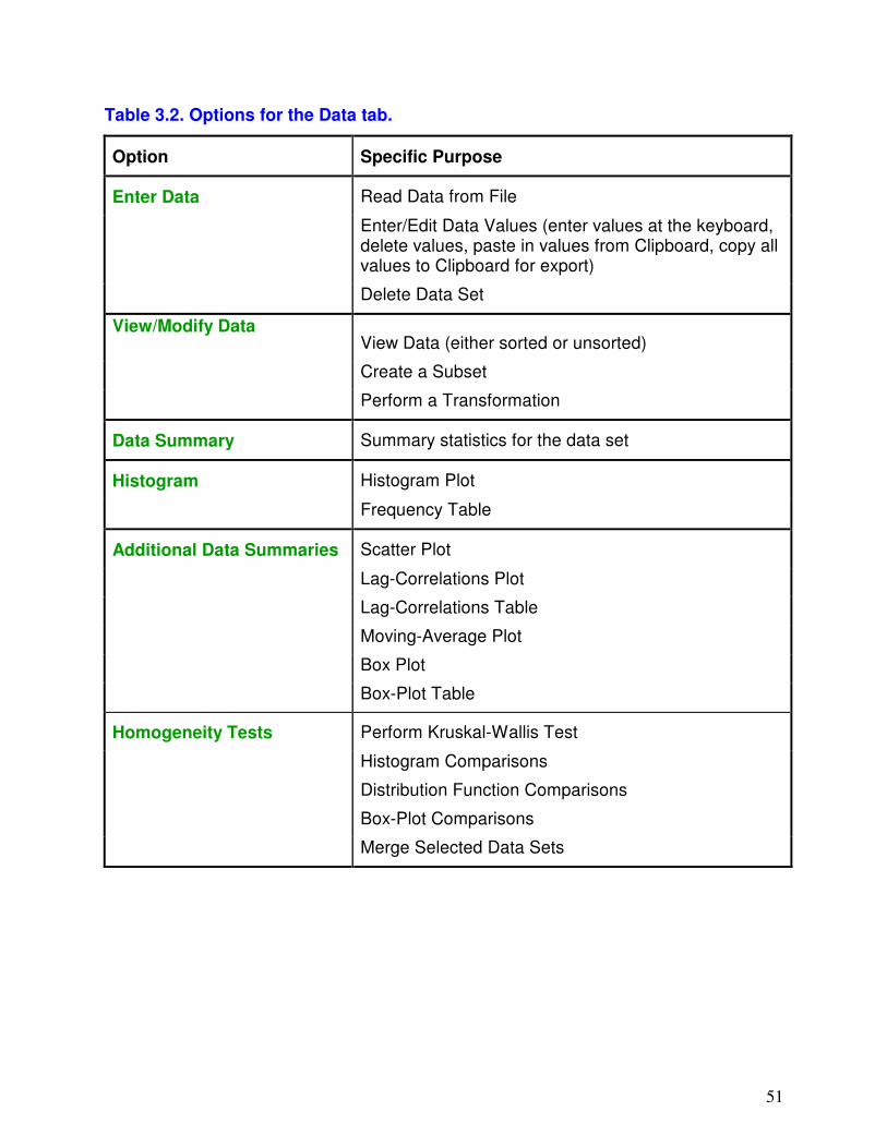
Table 3.2. Options for the Data tab.
Option Specific Purpose
Enter Data Read Data from File
Enter/Edit Data Values (enter values at the keyboard, delete values, paste in values from Clipboard, copy all values to Clipboard for export)
Delete Data Set
View/Modify Data View Data (either sorted or unsorted)
Create a Subset
Perform a Transformation
Data Summary Summary statistics for the data set
Histogram Histogram Plot
Frequency Table
Additional Data Summaries Scatter Plot
Lag-Correlations Plot
Lag-Correlations Table
Moving-Average Plot
Box Plot
Box-Plot Table
Homogeneity Tests Perform Kruskal-Wallis Test
Histogram Comparisons
Distribution Function Comparisons
Box-Plot Comparisons
Merge Selected Data Sets
52
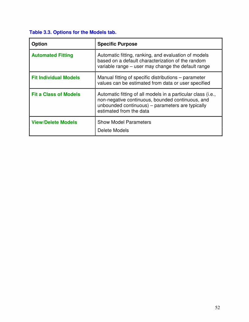
Table 3.3. Options for the Models tab.
Option Specific Purpose
Automated Fitting
Automatic fitting, ranking, and evaluation of models based on a default characterization of the random variable range – user may change the default range
Fit Individual Models Manual fitting of specific distributions – parameter values can be estimated from data or user specified
Fit a Class of Models Automatic fitting of all models in a particular class (i.e., non-negative continuous, bounded continuous, and unbounded continuous) – parameters are typically estimated from the data
View/Delete Models Show Model Parameters
Delete Models
53
Table 3.4. Options for the Comparisons tab.
Option Specific Purpose
Histogram Comparisons Density-Histogram Plot (real data only)
Frequency-Comparison Plot
Frequency-Comparison Table
Raw-Error Plot
Absolute-Error Plot
Table of Errors
Distribution Comparisons Distribution-Function-Differences Plot
Table of Errors
Distribution Function Plot
Survivor Function Plot
Probability Plots P-P Plot
Q-Q Plot (real data only)
Relative-Discrepancies Table
Goodness-of-Fit Tests Anderson-Darling Test (real data only)
Kolmogorov-Smirnov Test (real data only)
Equal-Probable Chi-Square Test
Equal-Width Chi-Square Test
Test-Statistics Comparison (real data only)
Additional Comparisons Moment-Comparison Table
Box-Plot Comparisons Plot (real data only)
Box-Plot Comparisons Percentile Table (real data only)
Likelihood-Function Table
Evaluate a Model Evaluation Report
Distribution-Function-Differences Plot
54
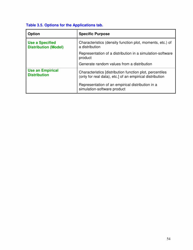
Table 3.5. Options for the Applications tab.
Option Specific Purpose
Use a Specified Distribution (Model)
Characteristics (density function plot, moments, etc.) of a distribution
Representation of a distribution in a simulation-software product
Generate random values from a distribution
Use an Empirical Distribution
Characteristics [distribution function plot, percentiles (only for real data), etc.] of an empirical distribution
Representation of an empirical distribution in a simulation-software product
55
Although there are different ways that these four tabs could be used to
determine the best distribution for a data set, the following are the explicit steps that we
recommend (same as for Standard Mode):
1. Obtain a data set using the Data tab – see Section 1.2 for a discussion of the type
and amount of data required.
2. View the resulting Data-Summary Table (at the Data tab) – provides information on
the center, shape, and range of the true density (mass) function.
3. Make a histogram of your data (used in Step 5) using the Data tab – see the
Constructing a Histogram from Your Data tutorial in the online help.
4. Select the distribution that is the best representation for your data using the
Automated Fitting option at the Models tab.
5. Confirm using the Comparisons tab that the best distribution as determined by
ExpertFit is, in fact, satisfactory in an absolute sense – see Section 2.1 for
recommendations.
6. If you are doing simulation modeling, then either represent the best-fitting
distribution (if good in an absolute sense) or an empirical distribution based on your
data (if the best distribution is not satisfactory) in your simulation software using the
Applications tab.
An example of the use of Advanced Mode for the Data Analysis module is
given in Section 3.1.
56
3.1. Example
We now present an example of the use of Advanced Mode for the Data
Analysis module, following the six-step approach outlined at the beginning of this
chapter. We use Normal Precision in fitting distributions to the data.
57
Example 3.1: Testing the Homogeneity of Two or More Data Sets
It is sometimes of interest to determine whether two or more “similar” data sets
are homogeneous. If the data sets are homogeneous, they can be merged. We can
then attempt to fit a single distribution to the merged data set.
Consider processing times corresponding to two different machines from the
same vendor. The data from machine 1, Example 3.1-1, contains 910 observations
and the data from machine 2, Example 3.1-2, contains 838 observations. We would
like to determine whether these data sets are homogeneous and, thus, can be merged.
Select the data set Example 3.1-1 in the Project EXAMPLES.EFP that comes with
ExpertFit. Now select Homogeneity Tests at the Data tab (for Advanced Mode) and
data set Example 3.1-2 from the scroll list of available data sets. We are now ready to
determine if the two selected data sets are homogeneous.
We first perform the Kruskal-Wallis test [see Law (2007, p. 380)] at level 0.05.
Since the test statistic, 0.004, is less than the critical value, 3.841 for 1 degree of
freedom, we cannot reject the hypothesis that the two data sets are homogeneous.
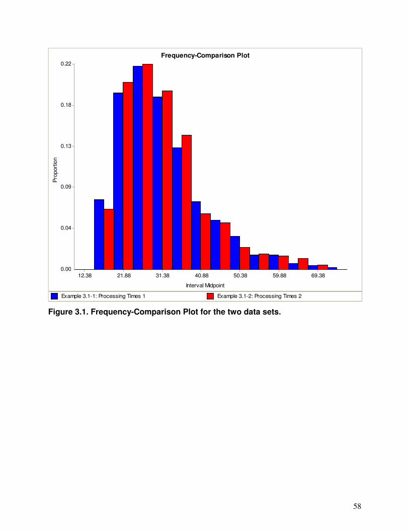
We next display a Frequency-Comparison Plot (see Histogram Comparisons
for Homogeneity Tests) for the two data sets, which plots histograms of both data sets
on the same graph. The common histograms, which start at 10 and have 14 intervals of
width 4.75, are shown in Figure 3.1. The similarity of the two histograms supports the
homogeneity of the two data sets.
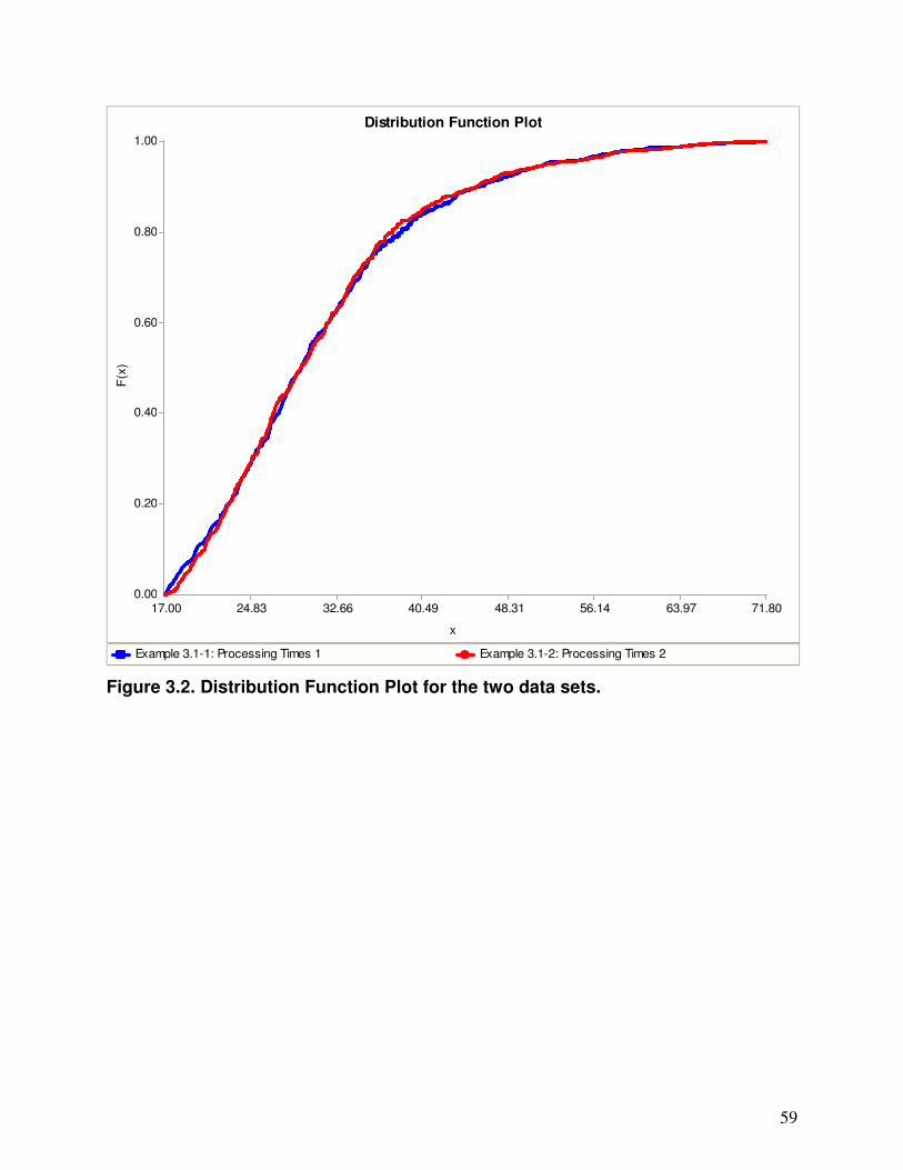
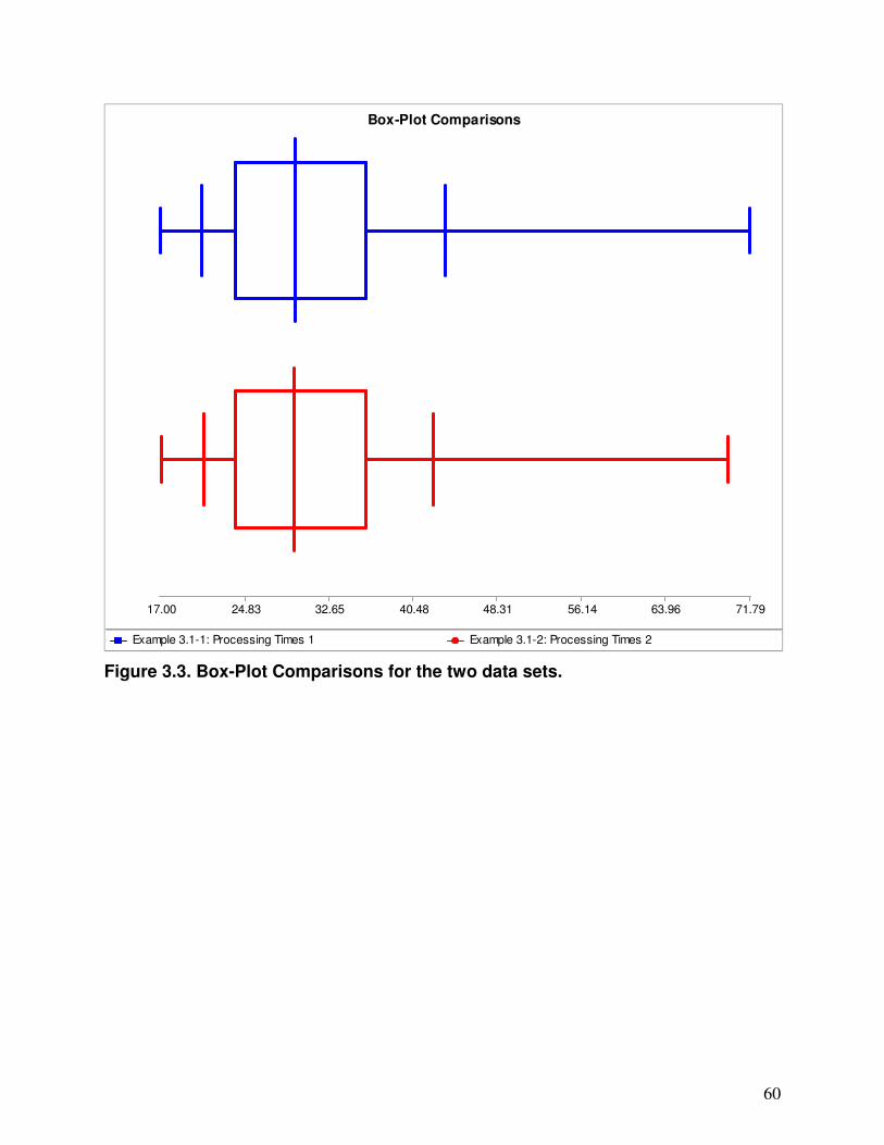
Finally, we display a Distribution Function Plot and a Box-Plot Comparisons
for the two data sets in Figures 3.2 and 3.3, respectively. These plots also support
homogeneity.
In conclusion, there is no reason to believe that the two data sets are not
homogeneous, and we merge them by clicking on the Merge Selected Data Sets
option. The merged data set is added to the current Project and is named Merged
data set. However, the name of this data set can be changed by closing the current
data analysis (i.e., for the data set Example 3.1-1) and clicking on the Edit button.
58
Example 3.1-1: Processing Times 1 Example 3.1-2: Processing Times 2
Figure 3.1. Frequency-Comparison Plot for the two data sets.
59
Example 3.1-1: Processing Times 1 Example 3.1-2: Processing Times 2
0.00
0.20
0.40
0.60
0.80
1.00
17.00 24.83 32.66 40.49 48.31 56.14 63.97 71.80
F(x
)Distribution Function PlotDistribution Function Plot
x
Figure 3.2. Distribution Function Plot for the two data sets.
60
Example 3.1-1: Processing Times 1 Example 3.1-2: Processing Times 2
17.00 24.83 32.65 40.48 48.31 56.14 63.96 71.79
Box-Plot ComparisonsBox-Plot Comparisons
Figure 3.3. Box-Plot Comparisons for the two data sets.
61
We now use Automated Fitting (with Normal Precision) to determine what
distribution best represents the Merged data set, which consists of 1748 observations.
It turns out that the Pearson type V distribution provides the best fit with a Relative
Score of 97.92. The Absolute Evaluation is “Indeterminate,” which means that more
evaluations need to be performed at the Comparisons tab before the quality of the
representation provided by the Pearson type V distribution can be determined. The
Anderson-Darling test says to reject the Pearson type V distribution at level 0.05;
however, for this large sample size, the test is very powerful and may reject a
hypothesized distribution whose error may be practically insignificant. In fact, the
Density-Histogram Plot, the Distribution Function Plot, the Distribution-Function-
Differences Plot, and the P-P Plot all indicate that the Pearson type V distribution
provides a reasonably good representation of the data.
62
4. Task-Time Models Module
In some simulation studies it is not possible to obtain good data on the random
variables of interest, so the usual statistical techniques are not applicable to the
problem of selecting corresponding probability distributions. For example, if the system
being studied does not currently exist in some form, collecting data from the system is
obviously not possible. This difficulty can also occur for existing systems, if the number
of required probability distributions is large and the time available for the simulation
study prohibits the necessary data collection and analysis. In addition, sometimes there
are data available from an existing system, but the data are not in a format suitable for
use in a simulation model (e.g., the data were collected by an automated system). For
such situations ExpertFit provides guidance on modeling a task time in the Task-Time
Models module. Note that the use of no-data models is not a substitute for a careful
analysis of data collected from your system, if this is possible.
Consider the continuous random variable corresponding to the time to complete
some task (e.g., a machine repair time or a customer service time in a bank). ExpertFit
allows you to model such a random variable by a Weibull, lognormal, or triangular
distribution. For a particular distribution, you must give subjective estimates of the
minimum task time, the most-likely task time (the mode), and the 100pth percentile of
the task time. Allowable percentiles for the Weibull and lognormal distributions are the
90th (the default), 95th, and 99th; the 100th percentile (the maximum value) is also
available for the triangular distribution. More information on the use of the Task-Time
Models module can be found in the Modeling Task Times in the Absence of Data
tutorial, which is accessed from the Help pull-down menu in ExpertFit.
After completely specifying a task-time model, you can display characteristics of
the model such as its density function or percentiles. You can also represent the task-
time model in the simulation-software product of your choice.
63
4.1. Organization and Options
A Task-Time Model is based on the sequential use of the two tabs given in
Table 4.1.
The options for the Models and Applications tabs are given in Tables 4.2 and
4.3, respectively.
Table 4.1. Tabs for the Task-Time Models module.
Tab Overall Purpose
Models Used to construct models for a task time
Applications Used to determine or display characteristics (e.g., density function) of specified models or to represent the models in a simulation-software product
Table 4.2. Options for the Models tab.
Option Specific Purpose
Specify a Model Used to create new (or to modify existing) models for a task time
View/Delete Models Used to display the parameters of currently specified models or to delete models
64
Table 4.3. Options for the Applications tab.
Option Specific Purpose
Characteristics Density Function Plot
Distribution Function Plot
Moment Table
Percentile Table
Probability for an x
Percentile for a p
Simulation Representation
Representation of a model in a simulation-software product
65
4.2. Example
In this section we present an example of the use of the Task-Time Models module.
66
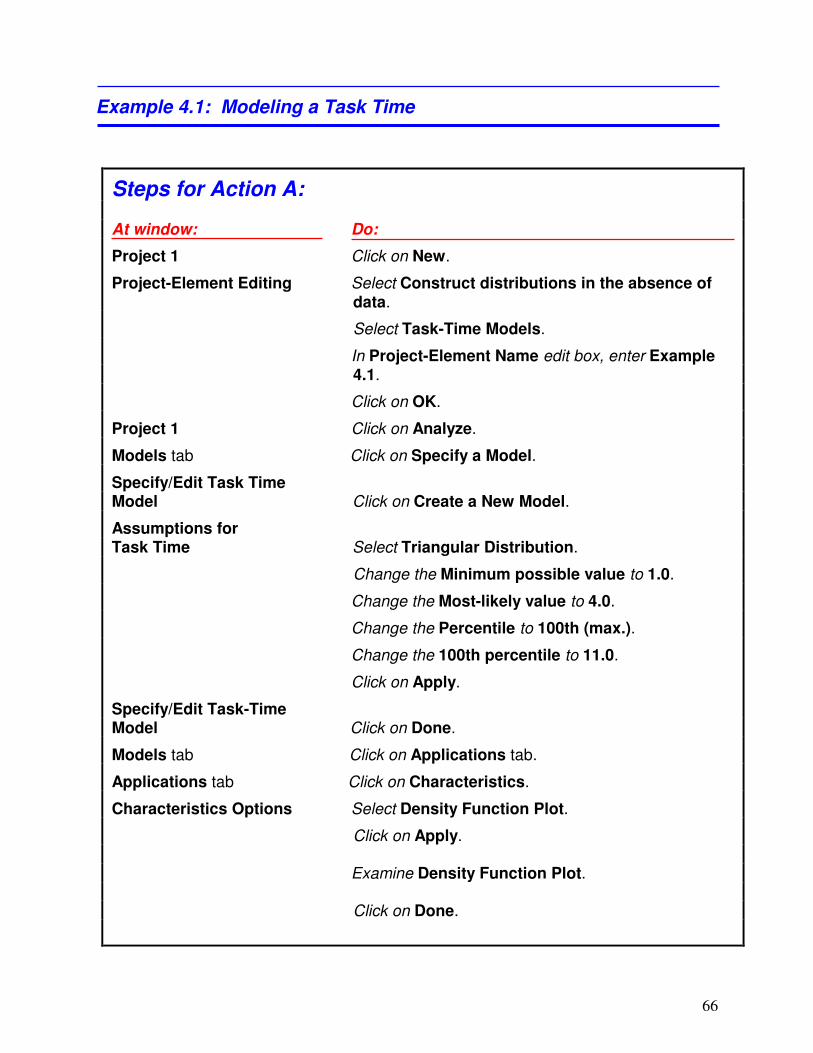
Example 4.1: Modeling a Task Time
Steps for Action A: At window: Do:
Project 1 Click on New.
Project-Element Editing Select Construct distributions in the absence of data.
Select Task-Time Models.
In Project-Element Name edit box, enter Example 4.1.
Click on OK.
Project 1 Click on Analyze.
Models tab Click on Specify a Model.
Specify/Edit Task Time Model Click on Create a New Model.
Assumptions for Task Time Select Triangular Distribution.
Change the Minimum possible value to 1.0.
Change the Most-likely value to 4.0.
Change the Percentile to 100th (max.).
Change the 100th percentile to 11.0.
Click on Apply.
Specify/Edit Task-Time Model Click on Done.
Models tab Click on Applications tab.
Applications tab Click on Characteristics.
Characteristics Options Select Density Function Plot.
Click on Apply. Examine Density Function Plot. Click on Done.
67
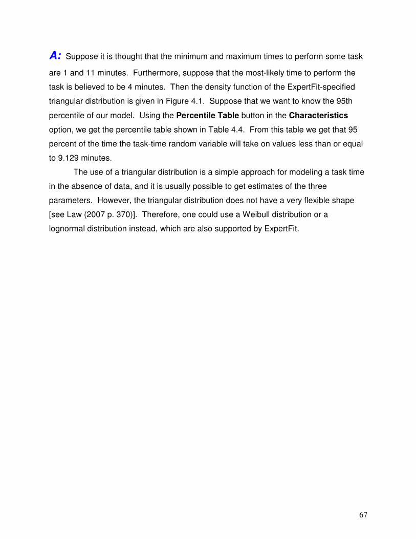
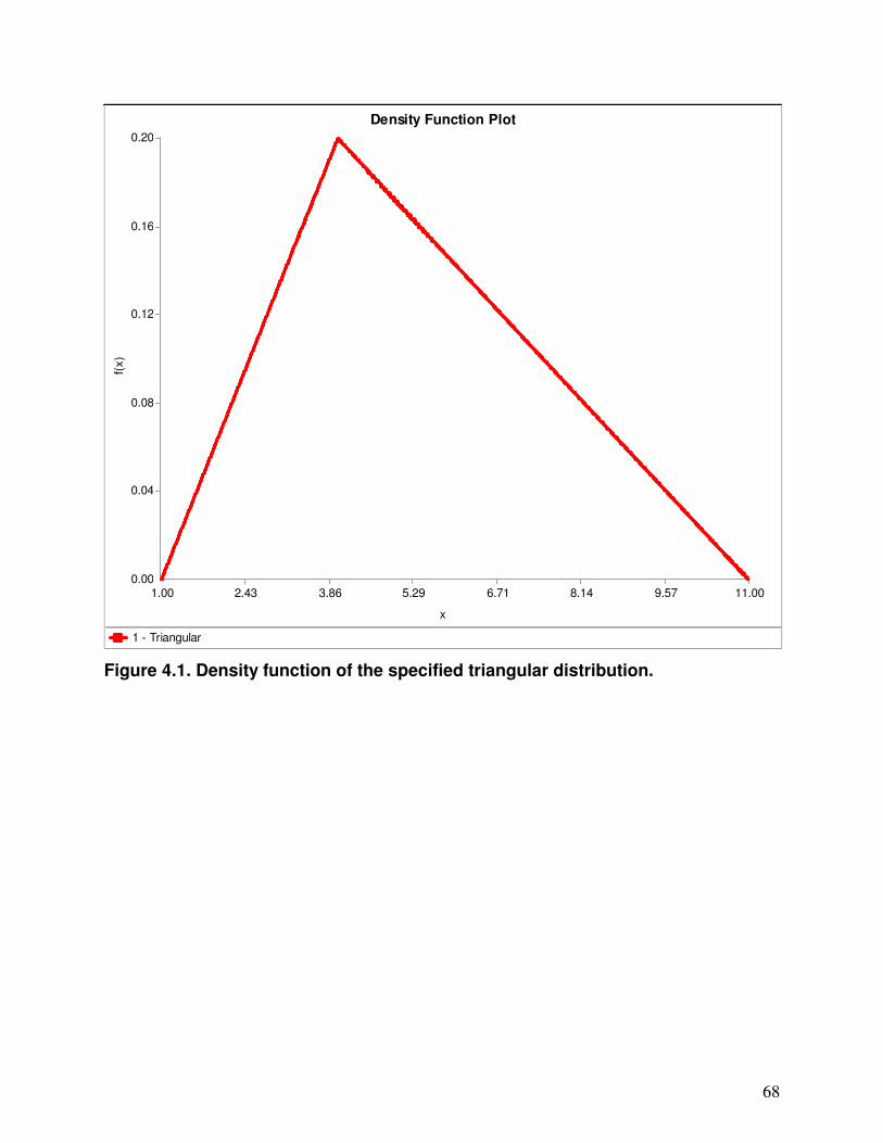
A: Suppose it is thought that the minimum and maximum times to perform some task
are 1 and 11 minutes. Furthermore, suppose that the most-likely time to perform the
task is believed to be 4 minutes. Then the density function of the ExpertFit-specified
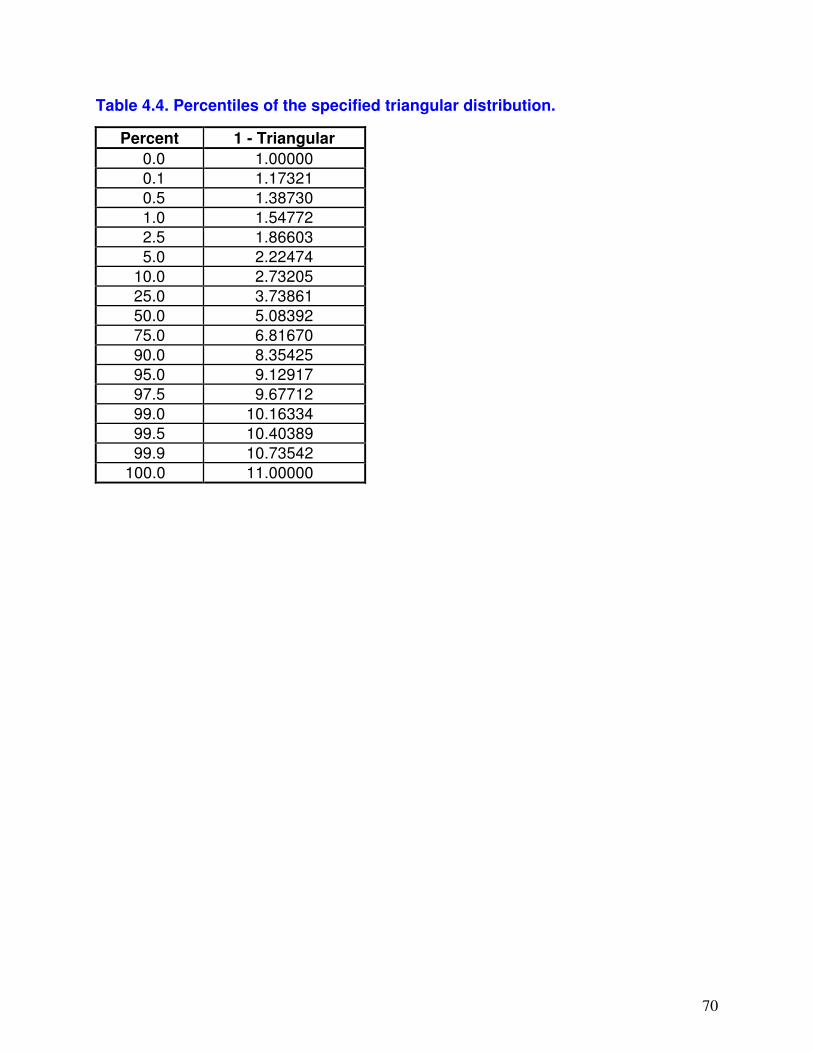
triangular distribution is given in Figure 4.1. Suppose that we want to know the 95th
percentile of our model. Using the Percentile Table button in the Characteristics
option, we get the percentile table shown in Table 4.4. From this table we get that 95
percent of the time the task-time random variable will take on values less than or equal
to 9.129 minutes.
The use of a triangular distribution is a simple approach for modeling a task time
in the absence of data, and it is usually possible to get estimates of the three
parameters. However, the triangular distribution does not have a very flexible shape
[see Law (2007 p. 370)]. Therefore, one could use a Weibull distribution or a
lognormal distribution instead, which are also supported by ExpertFit.
68
1 - Triangular
0.00
0.04
0.08
0.12
0.16
0.20
1.00 2.43 3.86 5.29 6.71 8.14 9.57 11.00
f(x)
Density Function PlotDensity Function Plot
x
Figure 4.1. Density function of the specified triangular distribution.
69
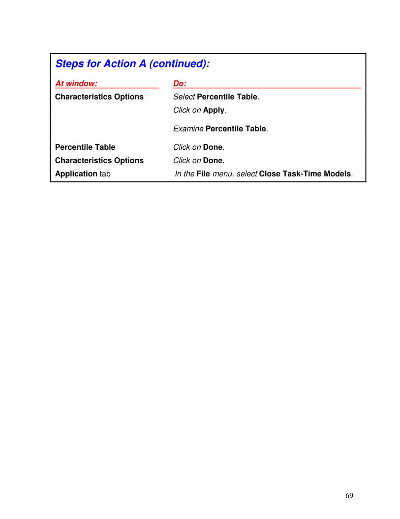
Steps for Action A (continued): At window: Do:
Characteristics Options Select Percentile Table.
Click on Apply. Examine Percentile Table. Percentile Table Click on Done.
Characteristics Options Click on Done.
Application tab In the File menu, select Close Task-Time Models.
70
Table 4.4. Percentiles of the specified triangular distribution.
Percent 1 - Triangular
0.0 1.00000
0.1 1.17321
0.5 1.38730
1.0 1.54772
2.5 1.86603
5.0 2.22474
10.0 2.73205
25.0 3.73861
50.0 5.08392
75.0 6.81670
90.0 8.35425
95.0 9.12917
97.5 9.67712
99.0 10.16334
99.5 10.40389
99.9 10.73542
100.0 11.00000
71
5. Machine-Breakdown Models Module
Representing the breakdown and repair of a machine in a simulation model is
considerably more complicated than just modeling a task time, since we have both
machine uptimes and downtimes to be concerned with. Also, the machine can be
starved (waiting for parts) or blocked (inability to remove a part from the machine) by
other machines downstream from it.
A machine goes through a sequence of cycles, with the jth cycle consisting of an
up segment (machine is operational) of length Uj, followed by a down segment of length
Dj. During an up segment, a machine will process parts if any are available and if the
machine is not blocked. The first two up-down cycles for a machine are shown in
Figure 5.1. Let Bj and Ij be the amounts of time during Uj that the machine is busy
processing parts and that the machine is idle (either starved for parts or blocked by the
current finished part), respectively. Thus, Uj = Bj + Ij. Note that Bj and Ij may each
correspond to a number of separated time segments and, thus, are not represented in
Figure 5.1.
We will assume for simplicity that cycles are independent of each other and are
probabilistically identical. We will also assume that Uj and Dj are independent for all j.
ExpertFit will help you specify probability distributions for a busy time B and for a
downtime D.
End of cycle End of cycle 0
Time
U1 U2 D1 D2
Figure 5.1. Up-down cycles for a machine.
72
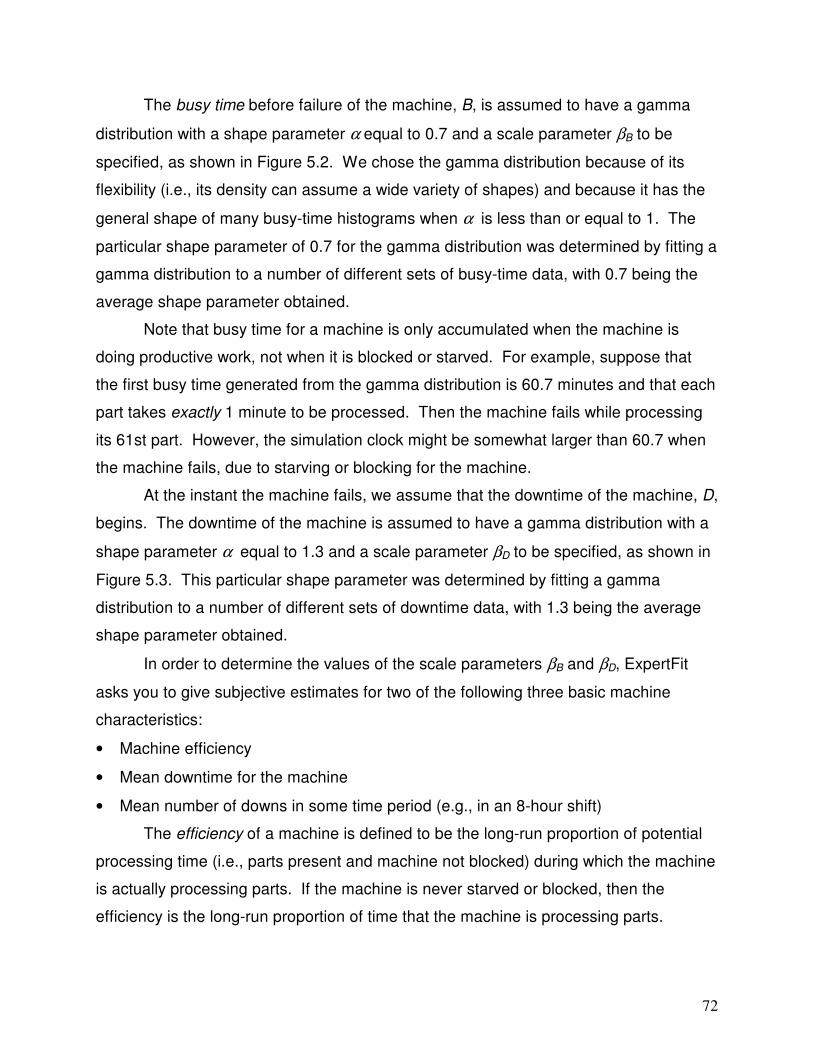
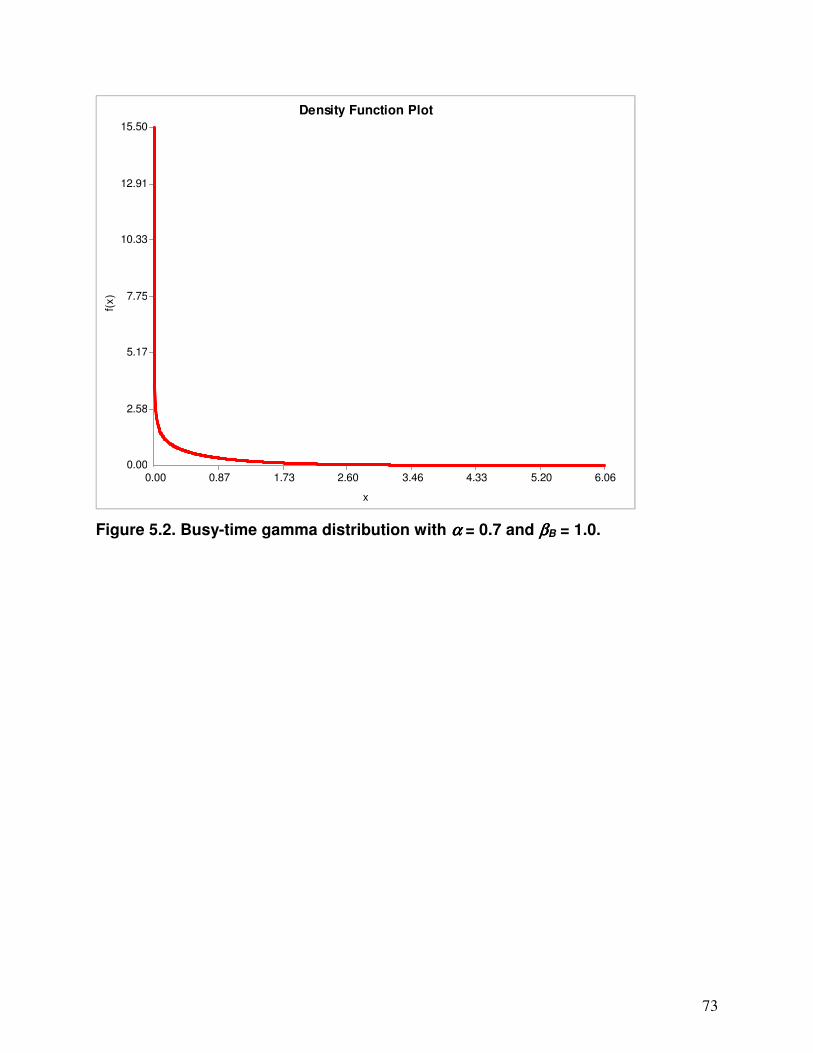
The busy time before failure of the machine, B, is assumed to have a gamma
distribution with a shape parameter α equal to 0.7 and a scale parameter βB to be
specified, as shown in Figure 5.2. We chose the gamma distribution because of its
flexibility (i.e., its density can assume a wide variety of shapes) and because it has the
general shape of many busy-time histograms when α is less than or equal to 1. The
particular shape parameter of 0.7 for the gamma distribution was determined by fitting a
gamma distribution to a number of different sets of busy-time data, with 0.7 being the
average shape parameter obtained.
Note that busy time for a machine is only accumulated when the machine is
doing productive work, not when it is blocked or starved. For example, suppose that
the first busy time generated from the gamma distribution is 60.7 minutes and that each
part takes exactly 1 minute to be processed. Then the machine fails while processing
its 61st part. However, the simulation clock might be somewhat larger than 60.7 when
the machine fails, due to starving or blocking for the machine.
At the instant the machine fails, we assume that the downtime of the machine, D,
begins. The downtime of the machine is assumed to have a gamma distribution with a
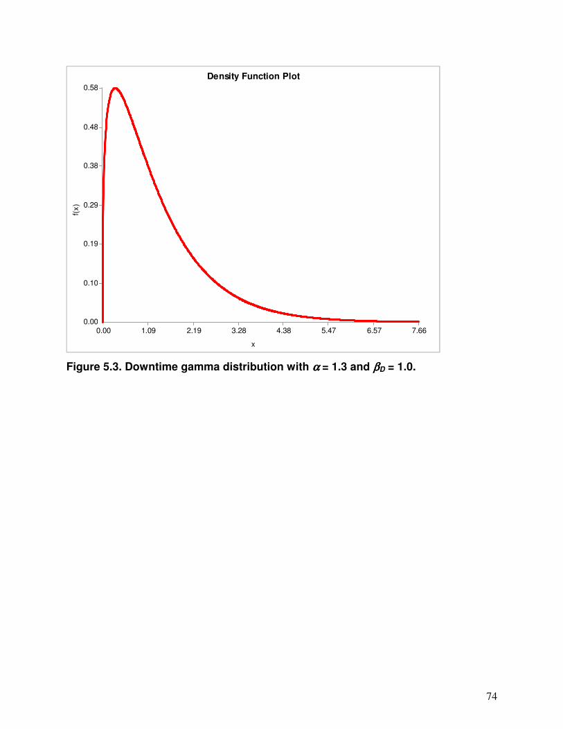
shape parameter α equal to 1.3 and a scale parameter βD to be specified, as shown in
Figure 5.3. This particular shape parameter was determined by fitting a gamma
distribution to a number of different sets of downtime data, with 1.3 being the average
shape parameter obtained.
In order to determine the values of the scale parameters βB and βD, ExpertFit
asks you to give subjective estimates for two of the following three basic machine
characteristics:
• Machine efficiency
• Mean downtime for the machine
• Mean number of downs in some time period (e.g., in an 8-hour shift)
The efficiency of a machine is defined to be the long-run proportion of potential
processing time (i.e., parts present and machine not blocked) during which the machine
is actually processing parts. If the machine is never starved or blocked, then the
efficiency is the long-run proportion of time that the machine is processing parts.
73
0.00
2.58
5.17
7.75
10.33
12.91
15.50
0.00 0.87 1.73 2.60 3.46 4.33 5.20 6.06
f(x)
Density Function PlotDensity Function Plot
x
Figure 5.2. Busy-time gamma distribution with αααα = 0.7 and ββββB = 1.0.
74
0.00
0.10
0.19
0.29
0.38
0.48
0.58
0.00 1.09 2.19 3.28 4.38 5.47 6.57 7.66
f(x)
Density Function PlotDensity Function Plot
x
Figure 5.3. Downtime gamma distribution with αααα = 1.3 and ββββD = 1.0.
75
The mean downtime of a machine is the mean amount of time that elapses from
the instant the machine breaks down until the instant that it is repaired; it includes both
the time spent waiting for a repairman (if any) and the repair time itself.
The mean number of downs in some time period (called the Time Frame in
ExpertFit) such as a shift (possibly, non integral) is, more specifically, the mean number
of busy-time/downtime cycles in a time period. For example, if the mean number of
downs is exactly 2, then the machine fails and is subsequently repaired an average of 2
times in a time period.
If the machine is subject to significant starving or blocking, then you must also
give the mean number of parts produced per time period and the mean part-processing
time in order for ExpertFit to compute βB and βD.
The default gamma distributions used for busy time and downtime have location
parameters of zero; thus, they can take on arbitrarily small positive values. However, in
practice one or both of these distributions might have a minimum possible value (i.e., its
location parameter) that is a positive number. For example, it might be known that the
minimum possible downtime is 10 minutes. Thus, ExpertFit allows you to specify a
positive value for the minimum possible downtime or for the minimum possible busy
time.
76
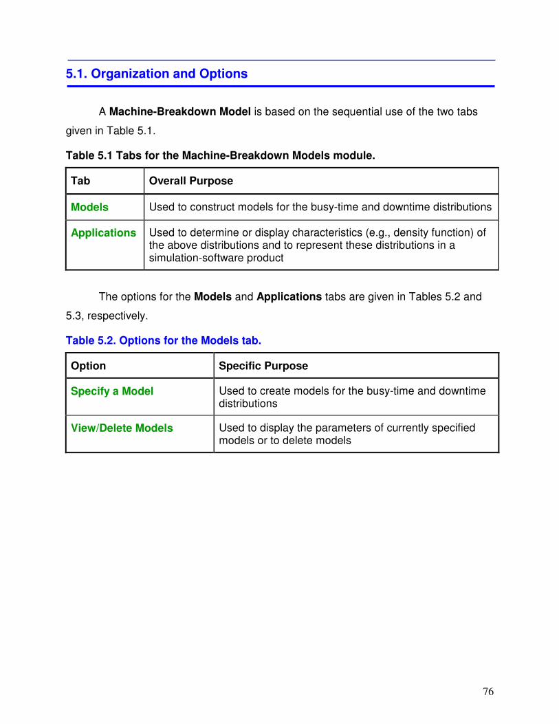
5.1. Organization and Options
A Machine-Breakdown Model is based on the sequential use of the two tabs
given in Table 5.1.
The options for the Models and Applications tabs are given in Tables 5.2 and
5.3, respectively.
Table 5.1 Tabs for the Machine-Breakdown Models module.
Tab Overall Purpose
Models Used to construct models for the busy-time and downtime distributions
Applications Used to determine or display characteristics (e.g., density function) of the above distributions and to represent these distributions in a simulation-software product
Table 5.2. Options for the Models tab.
Option Specific Purpose
Specify a Model Used to create models for the busy-time and downtime distributions
View/Delete Models Used to display the parameters of currently specified models or to delete models
77
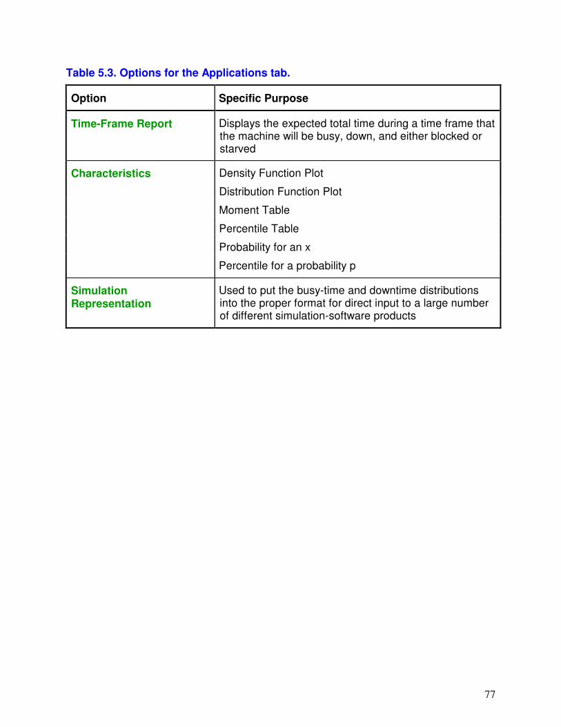
Table 5.3. Options for the Applications tab.
Option Specific Purpose
Time-Frame Report Displays the expected total time during a time frame that the machine will be busy, down, and either blocked or starved
Characteristics Density Function Plot
Distribution Function Plot
Moment Table
Percentile Table
Probability for an x
Percentile for a probability p
Simulation Representation
Used to put the busy-time and downtime distributions into the proper format for direct input to a large number of different simulation-software products
78
5.2. Examples
In this section we present two examples of the use of the Machine-Breakdown Models module.
79
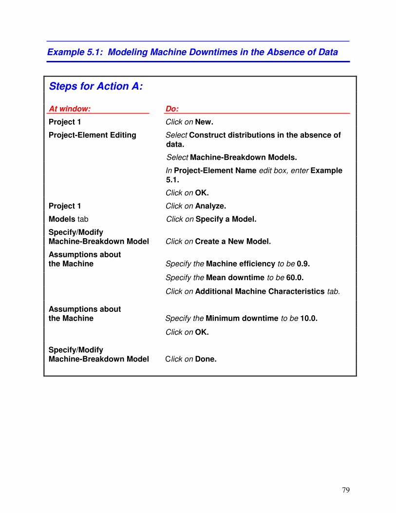
Example 5.1: Modeling Machine Downtimes in the Absence of Data
Steps for Action A: At window: Do:
Project 1 Click on New.
Project-Element Editing Select Construct distributions in the absence of data.
Select Machine-Breakdown Models.
In Project-Element Name edit box, enter Example 5.1.
Click on OK.
Project 1 Click on Analyze.
Models tab Click on Specify a Model.
Specify/Modify Machine-Breakdown Model Click on Create a New Model.
Assumptions about the Machine Specify the Machine efficiency to be 0.9.
Specify the Mean downtime to be 60.0.
Click on Additional Machine Characteristics tab.
Assumptions about the Machine Specify the Minimum downtime to be 10.0.
Click on OK.
Specify/Modify Machine-Breakdown Model Click on Done.
80
A: Consider a machine that is never starved or blocked. Suppose that the machine
has an efficiency of 0.9; that is, it is actually producing parts 90 percent of the time.
When the machine goes down, the mean downtime is 60 minutes. However, the
minimum possible downtime is 10 minutes. These characteristics are entered using
the commands on the previous page. Note that the default values for the Blocking
and/or Starving are Significant checkbox, Characteristics to be Entered, and
Time Unit are correct. Time Frame is not used in this example.
The machine busy-time and downtime distributions have now been completely
specified, and all of the specified and calculated (shown in blue) machine
characteristics are shown on the Specify/Modify Machine-Breakdown Model screen.
In particular, note that the mean number of downs (actually the mean number of busy-
time/downtime cycles) per 8-hour shift has been calculated to be 0.8. This makes
sense since the mean length of a busy-time/downtime cycle is 10 hours.
81
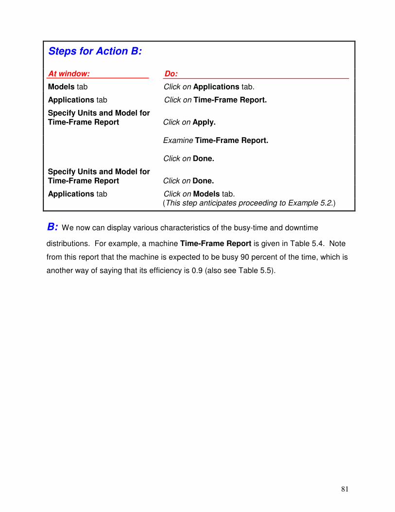
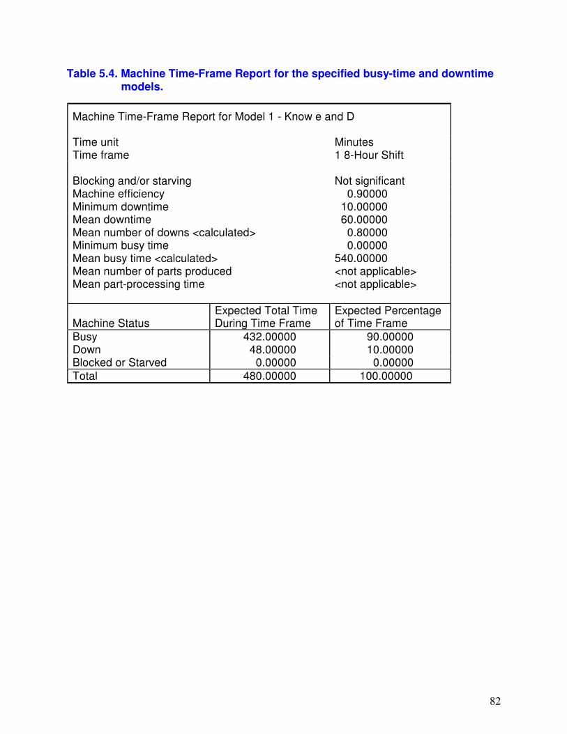
B: We now can display various characteristics of the busy-time and downtime
distributions. For example, a machine Time-Frame Report is given in Table 5.4. Note
from this report that the machine is expected to be busy 90 percent of the time, which is
another way of saying that its efficiency is 0.9 (also see Table 5.5).
Steps for Action B: At window: Do:
Models tab Click on Applications tab.
Applications tab Click on Time-Frame Report.
Specify Units and Model for Time-Frame Report Click on Apply. Examine Time-Frame Report. Click on Done.
Specify Units and Model for Time-Frame Report Click on Done.
Applications tab Click on Models tab. (This step anticipates proceeding to Example 5.2.)
82
Table 5.4. Machine Time-Frame Report for the specified busy-time and downtime models.
Machine Time-Frame Report for Model 1 - Know e and D Time unit Minutes Time frame 1 8-Hour Shift Blocking and/or starving Not significant Machine efficiency 0.90000 Minimum downtime 10.00000 Mean downtime 60.00000 Mean number of downs <calculated> 0.80000 Minimum busy time 0.00000 Mean busy time <calculated> 540.00000 Mean number of parts produced <not applicable> Mean part-processing time <not applicable>
Expected Total Time Expected Percentage Machine Status During Time Frame of Time Frame
Busy 432.00000 90.00000 Down 48.00000 10.00000 Blocked or Starved 0.00000 0.00000
Total 480.00000 100.00000
83
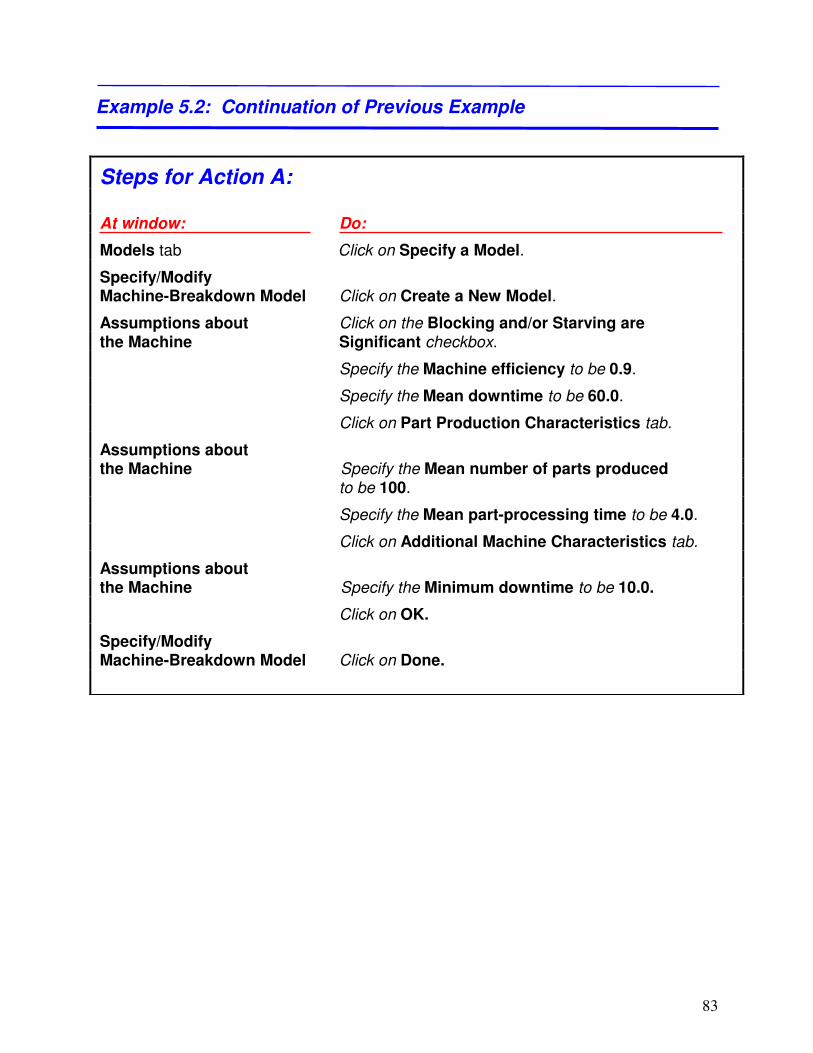
Example 5.2: Continuation of Previous Example
Steps for Action A: At window: Do:
Models tab Click on Specify a Model.
Specify/Modify Machine-Breakdown Model Click on Create a New Model.
Assumptions about Click on the Blocking and/or Starving are the Machine Significant checkbox.
Specify the Machine efficiency to be 0.9.
Specify the Mean downtime to be 60.0.
Click on Part Production Characteristics tab.
Assumptions about the Machine Specify the Mean number of parts produced to be 100.
Specify the Mean part-processing time to be 4.0.
Click on Additional Machine Characteristics tab.
Assumptions about the Machine Specify the Minimum downtime to be 10.0.
Click on OK.
Specify/Modify Machine-Breakdown Model Click on Done.
84
A: Suppose for the machine of Example 5.1 that blocking/starving is now significant.
For example raw materials might arrive to the machine on an intermittent basis.
Suppose also that the mean number of parts produced per 8-hour shift (the default
value of the Time Frame) is 100 and the mean part-processing time is 4 minutes.
We set the Blocking and/or Starving are Significant checkbox to “on” at the Basic
Machine Characteristics tab, in addition to specifying the Machine Efficiency and
Mean Downtime as in Example 5.1. Because blocking/starving is now significant, we
must specify values for Mean number of parts produced and Mean part-processing
time at the Part Production Characteristics tab. Finally, the Minimum downtime is
specified at the Additional Machine Characteristics tab.
85
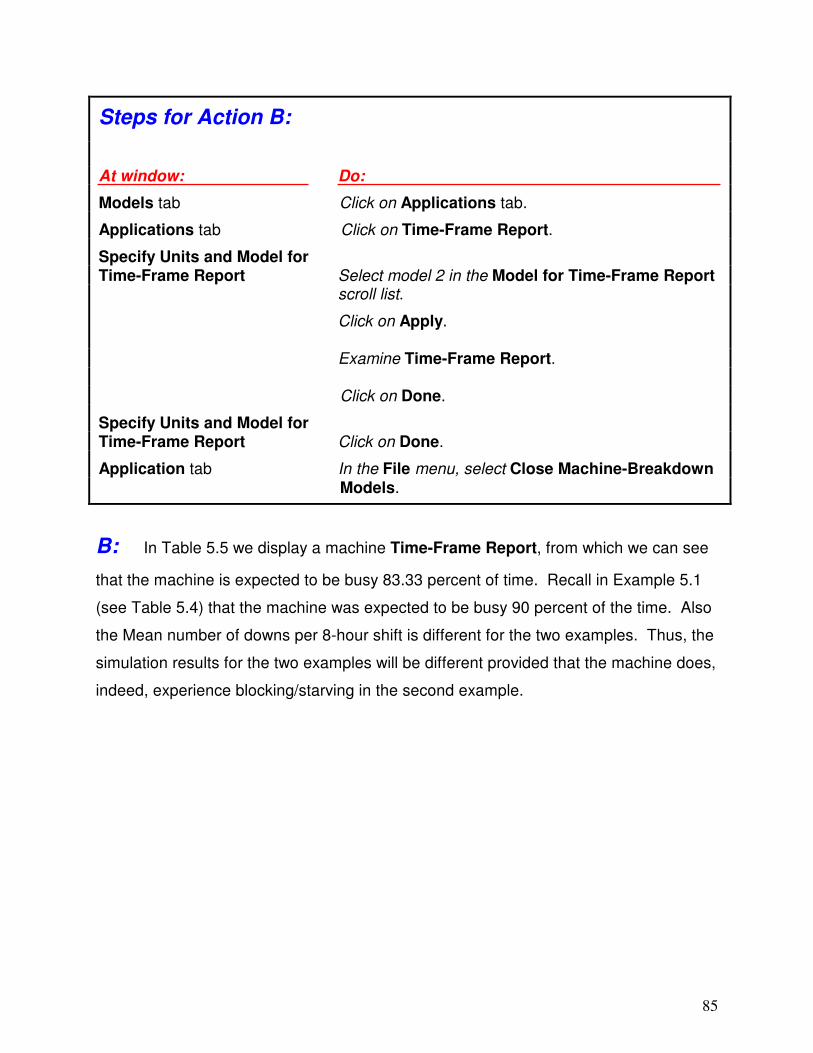
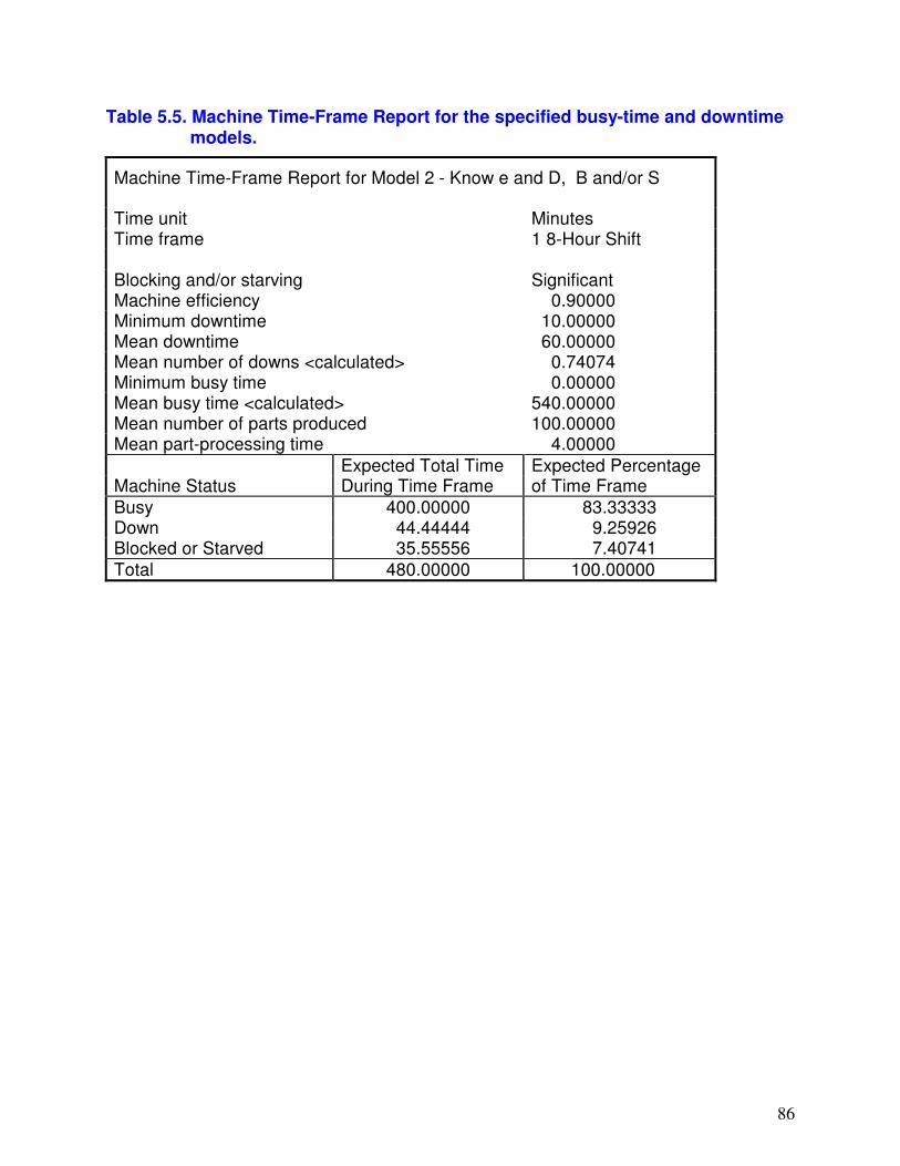
B: In Table 5.5 we display a machine Time-Frame Report, from which we can see
that the machine is expected to be busy 83.33 percent of time. Recall in Example 5.1
(see Table 5.4) that the machine was expected to be busy 90 percent of the time. Also
the Mean number of downs per 8-hour shift is different for the two examples. Thus, the
simulation results for the two examples will be different provided that the machine does,
indeed, experience blocking/starving in the second example.
Steps for Action B:
At window: Do:
Models tab Click on Applications tab.
Applications tab Click on Time-Frame Report.
Specify Units and Model for Time-Frame Report Select model 2 in the Model for Time-Frame Report scroll list.
Click on Apply. Examine Time-Frame Report. Click on Done.
Specify Units and Model for Time-Frame Report Click on Done.
Application tab In the File menu, select Close Machine-Breakdown Models.
86
Table 5.5. Machine Time-Frame Report for the specified busy-time and downtime models.
Machine Time-Frame Report for Model 2 - Know e and D, B and/or S Time unit Minutes Time frame 1 8-Hour Shift Blocking and/or starving Significant Machine efficiency 0.90000 Minimum downtime 10.00000 Mean downtime 60.00000 Mean number of downs <calculated> 0.74074 Minimum busy time 0.00000 Mean busy time <calculated> 540.00000 Mean number of parts produced 100.00000 Mean part-processing time 4.00000
Expected Total Time Expected Percentage Machine Status During Time Frame of Time Frame
Busy 400.00000 83.33333 Down 44.44444 9.25926 Blocked or Starved 35.55556 7.40741
Total 480.00000 100.00000
87
6. Distribution Viewer
The Distribution Viewer is used to display/calculate characteristics (e.g., the
density function or moments) of a distribution without having to enter a data set. It is
accessed from the Menu Bar at the top of the screen.
The distribution of interest is selected from the scroll list in the upper left-hand
corner of the screen and its density (or mass) function is displayed automatically for
default values of the distribution’s parameters. The parameters can be changed in the
following two ways:
• The value for a particular parameter can be entered in the corresponding data box.
[Click on the equal sign (“=”) and then enter a value.] In order to obtain a
meaningful density function plot, there are limits on the value of a parameter.
• A particular parameter can be changed dynamically by clicking on the “up” or “down”
button to the right of the data box. Clicking the up (down) button causes a real-
valued parameter to increase (decrease) by 0.1. (For an integer-valued parameter,
the change is 1 or –1.) Alternatively, a button can be held down to change the
parameter at a faster rate.
You can, in certain cases, choose to plot a density (or mass) function from either
its 0th or ath (e.g., a = 0.1) percentile to either its bth (e.g., b = 99.9) or 100th
percentile. Use of other than the 0th or the 100th percentile may be necessary to
obtain a plot that is not completely concentrated near the origin.
Additional information (e.g., moments, percentiles, and probabilities) about the
selected distribution can be obtained by clicking on the Other Options button in the
lower left-hand corner of the screen.
88
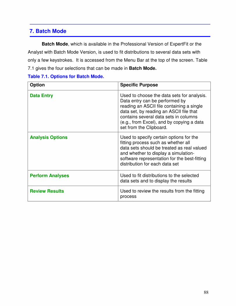
7. Batch Mode
Batch Mode, which is available in the Professional Version of ExpertFit or the
Analyst with Batch Mode Version, is used to fit distributions to several data sets with
only a few keystrokes. It is accessed from the Menu Bar at the top of the screen. Table
7.1 gives the four selections that can be made in Batch Mode.
Table 7.1. Options for Batch Mode.
Option Specific Purpose
Data Entry Used to choose the data sets for analysis. Data entry can be performed by reading an ASCII file containing a single data set, by reading an ASCII file that contains several data sets in columns (e.g., from Excel), and by copying a data set from the Clipboard.
Analysis Options Used to specify certain options for the fitting process such as whether all data sets should be treated as real valued and whether to display a simulation-software representation for the best-fitting distribution for each data set
Perform Analyses Used to fit distributions to the selected data sets and to display the results
Review Results Used to review the results from the fitting process
89
References
Evans, M., N. Hastings, and B. Peacock, Statistical Distributions, Third Edition, John Wiley, New York (2000).
Johnson, N. L., S. Kotz, and N. Balakrishnan, Continuous Univariate Distributions, Volume 1, Second Edition, Houghton Mifflin, Boston (1994).
Johnson, N. L., S. Kotz, and N. Balakrishnan, Continuous Univariate Distributions, Volume 2, Second Edition, Houghton Mifflin, Boston (1995).
Johnson, N. L., S. Kotz, and A.W. Kemp, Univariate Discrete Distributions, Second Edition, Houghton Mifflin, Boston (1992).
Law, A. M., Simulation Modeling and Analysis, Fourth Edition, McGraw-Hill, New York (2007).
90
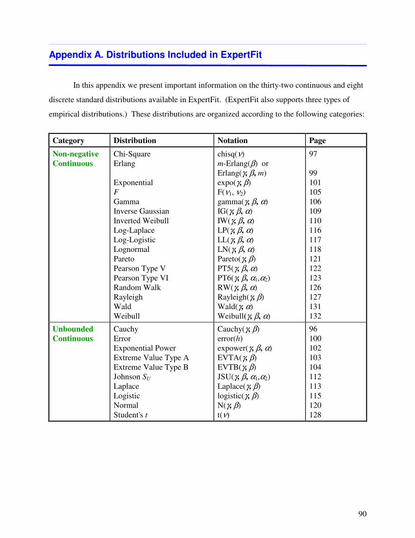
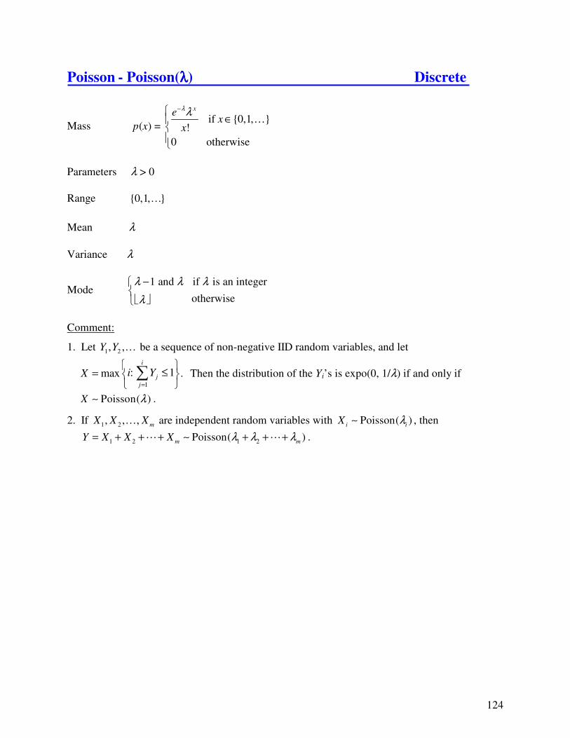
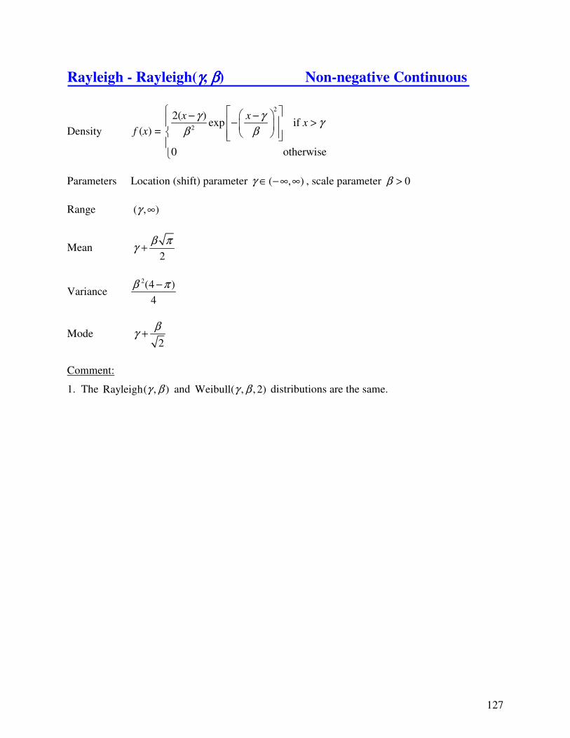
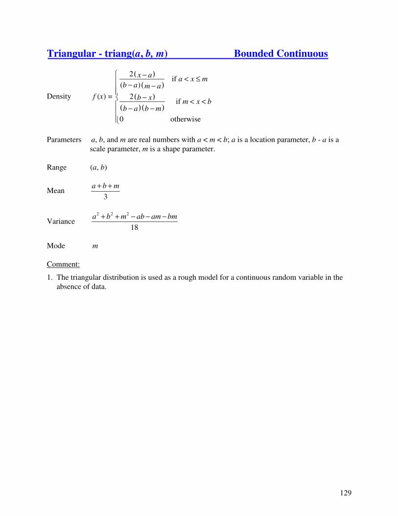
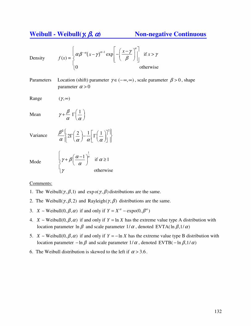
Appendix A. Distributions Included in ExpertFit
In this appendix we present important information on the thirty-two continuous and eight
discrete standard distributions available in ExpertFit. (ExpertFit also supports three types of
empirical distributions.) These distributions are organized according to the following categories:
Category Distribution Notation Page
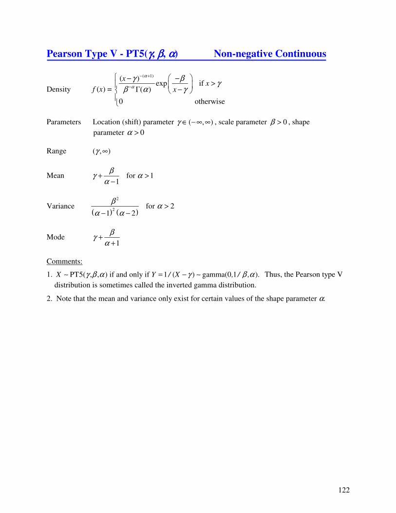
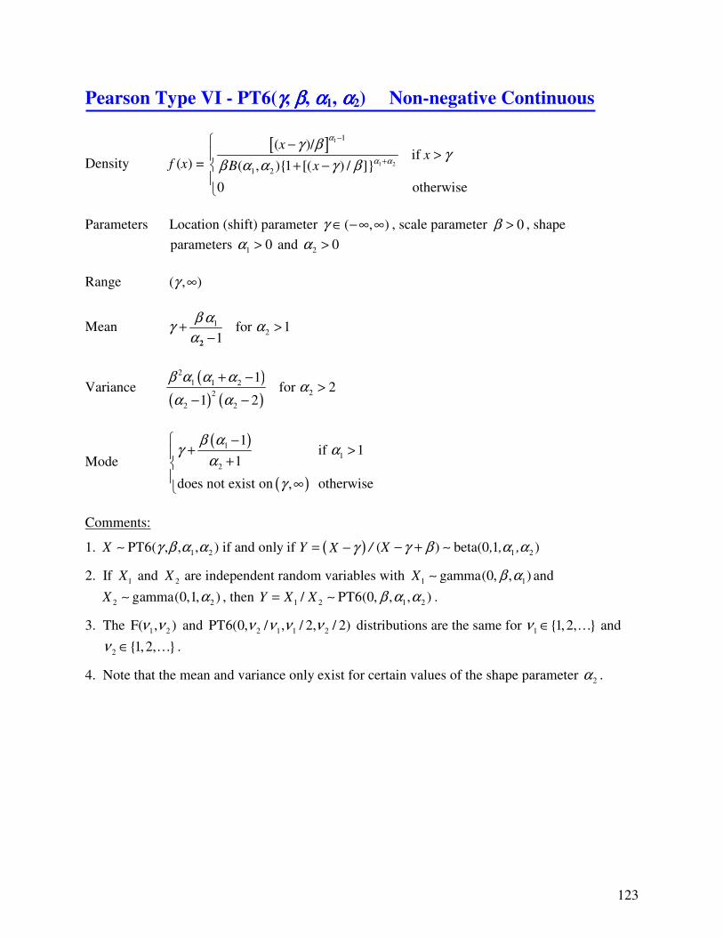
Non-negative
Continuous
Chi-Square
Erlang
Exponential
F
Gamma
Inverse Gaussian
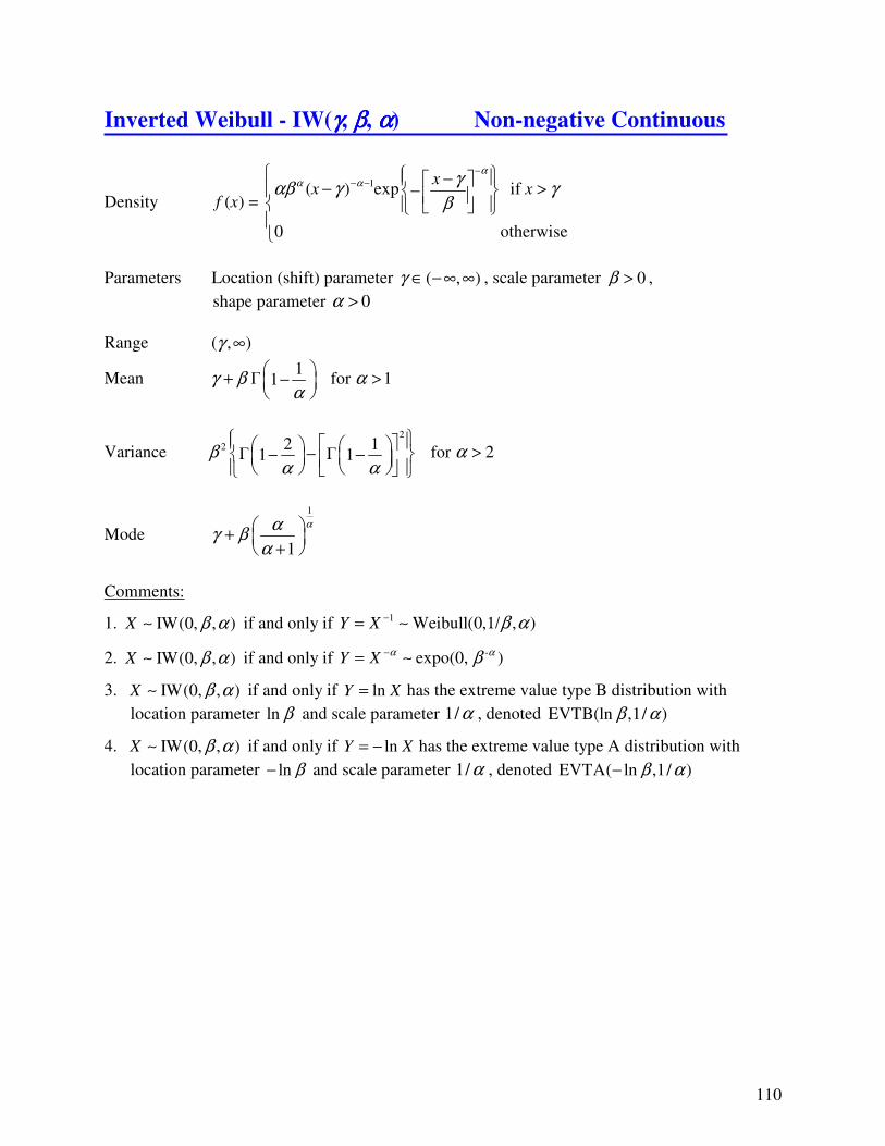
Inverted Weibull
Log-Laplace
Log-Logistic
Lognormal
Pareto
Pearson Type V
Pearson Type VI
Random Walk
Rayleigh
Wald
Weibull
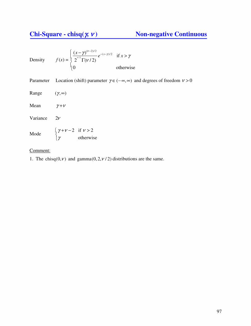
chisq(ν)
m-Erlang(β) or
Erlang(γ, β, m)
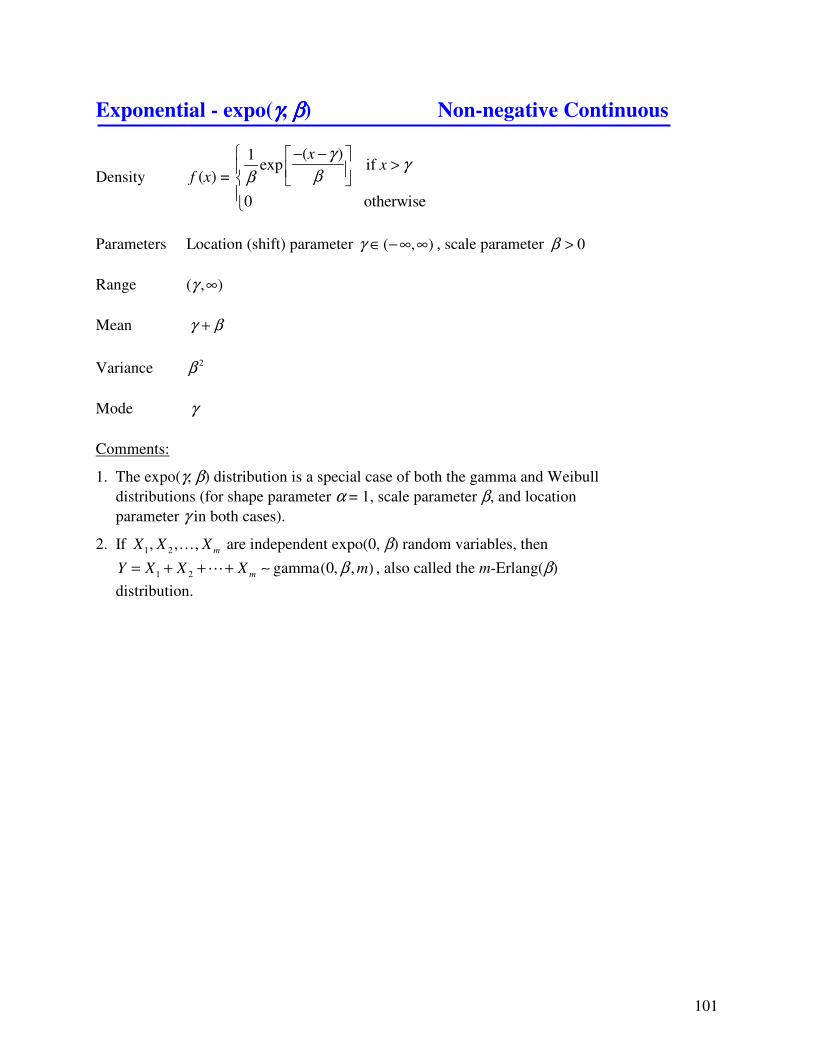
expo(γ, β)
F(ν1, ν2)
gamma(γ, β, α)
IG(γ, β, α)
IW(γ, β, α)
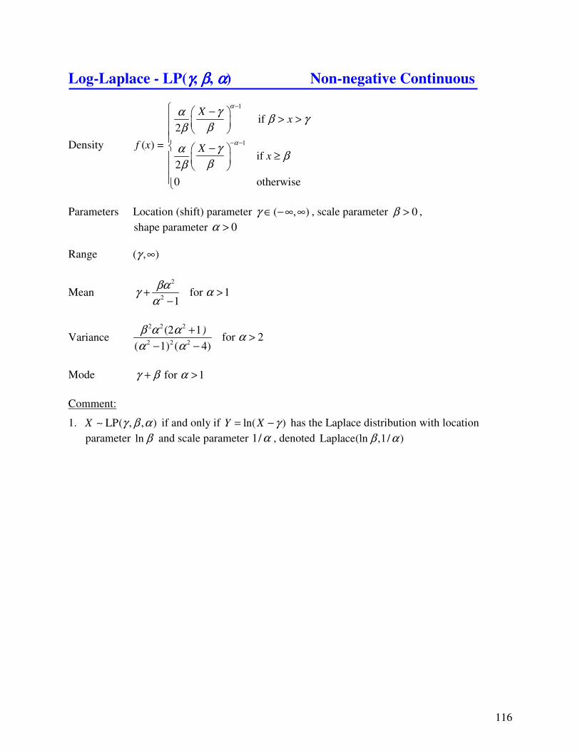
LP(γ, β, α)
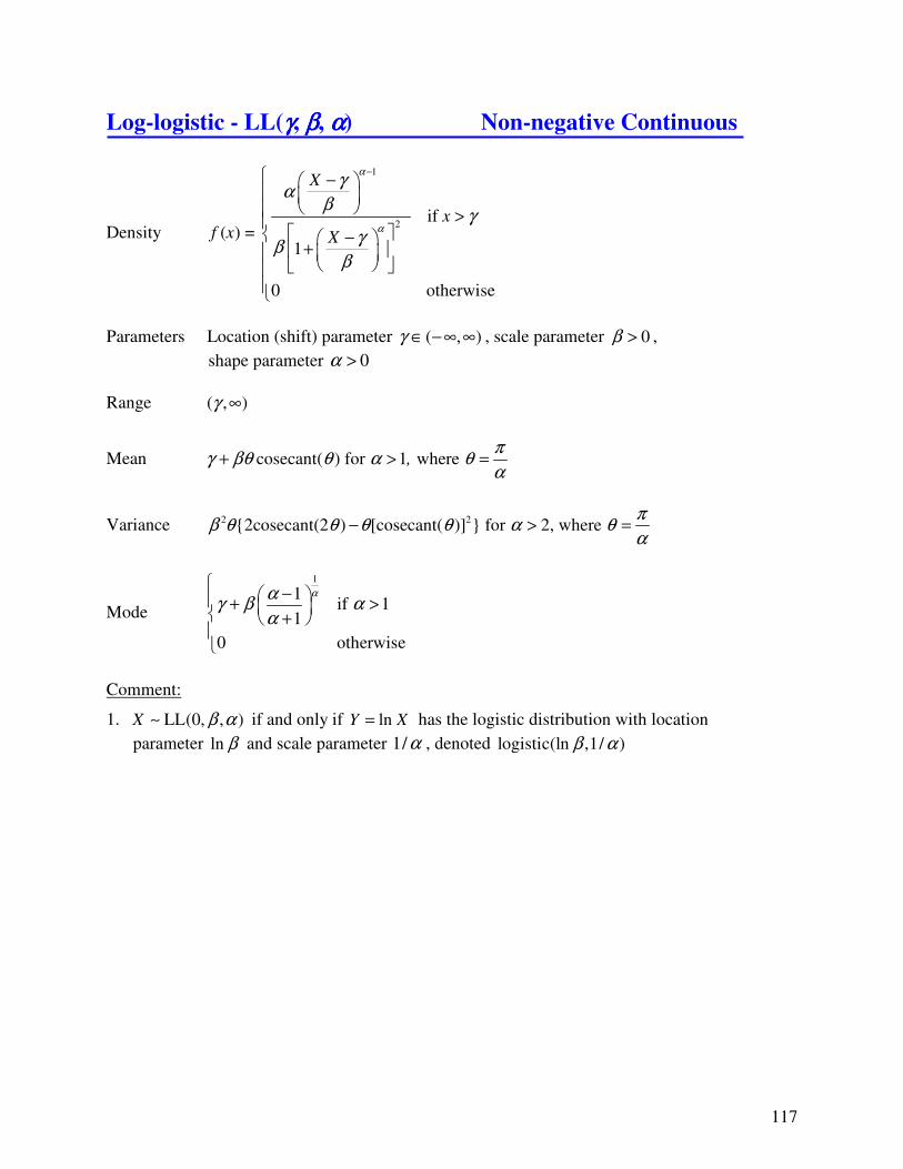
LL(γ, β, α)
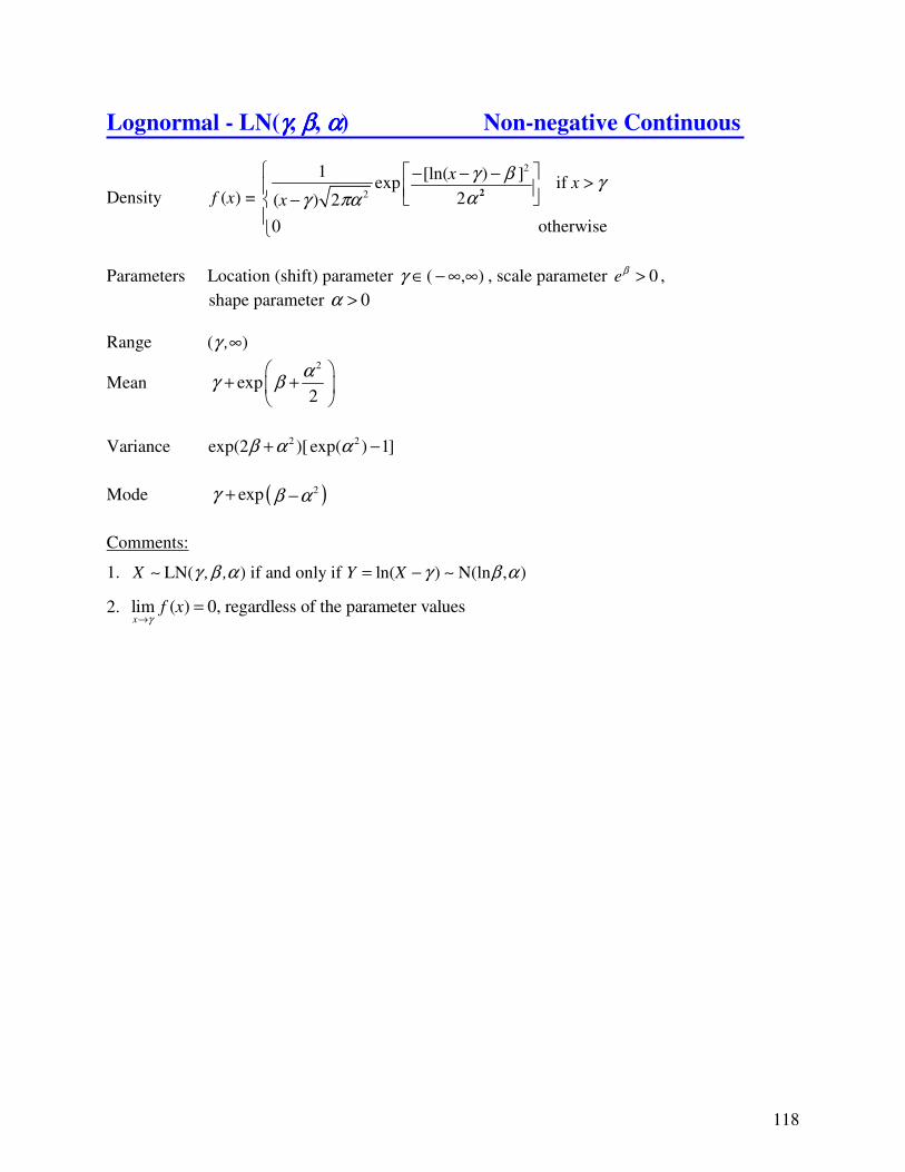
LN(γ, β, α)
Pareto(γ, β)
PT5(γ, β, α)
PT6(γ, β, α1,α2)
RW(γ, β, α)
Rayleigh(γ, β)
Wald(γ, α)
Weibull(γ, β, α)
97
99
101
105
106
109
110
116
117
118
121
122
123
126
127
131
132
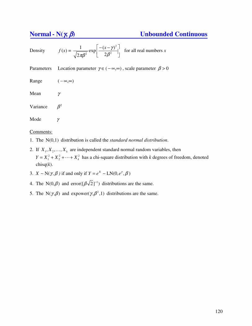
Unbounded
Continuous
Cauchy
Error
Exponential Power
Extreme Value Type A
Extreme Value Type B
Johnson SU
Laplace
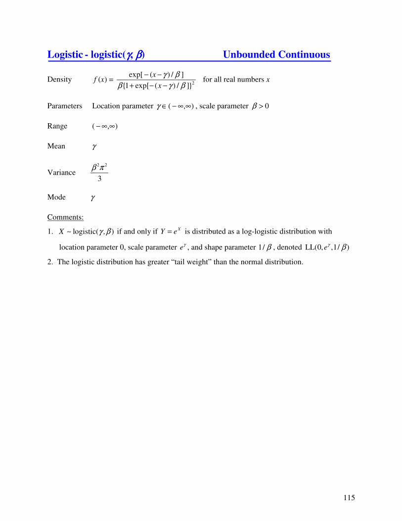
Logistic
Normal
Student's t
Cauchy(γ, β)
error(h)
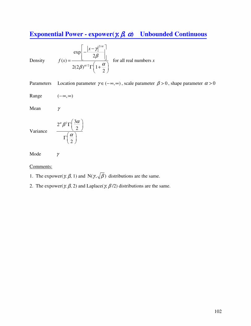
expower(γ, β, α)
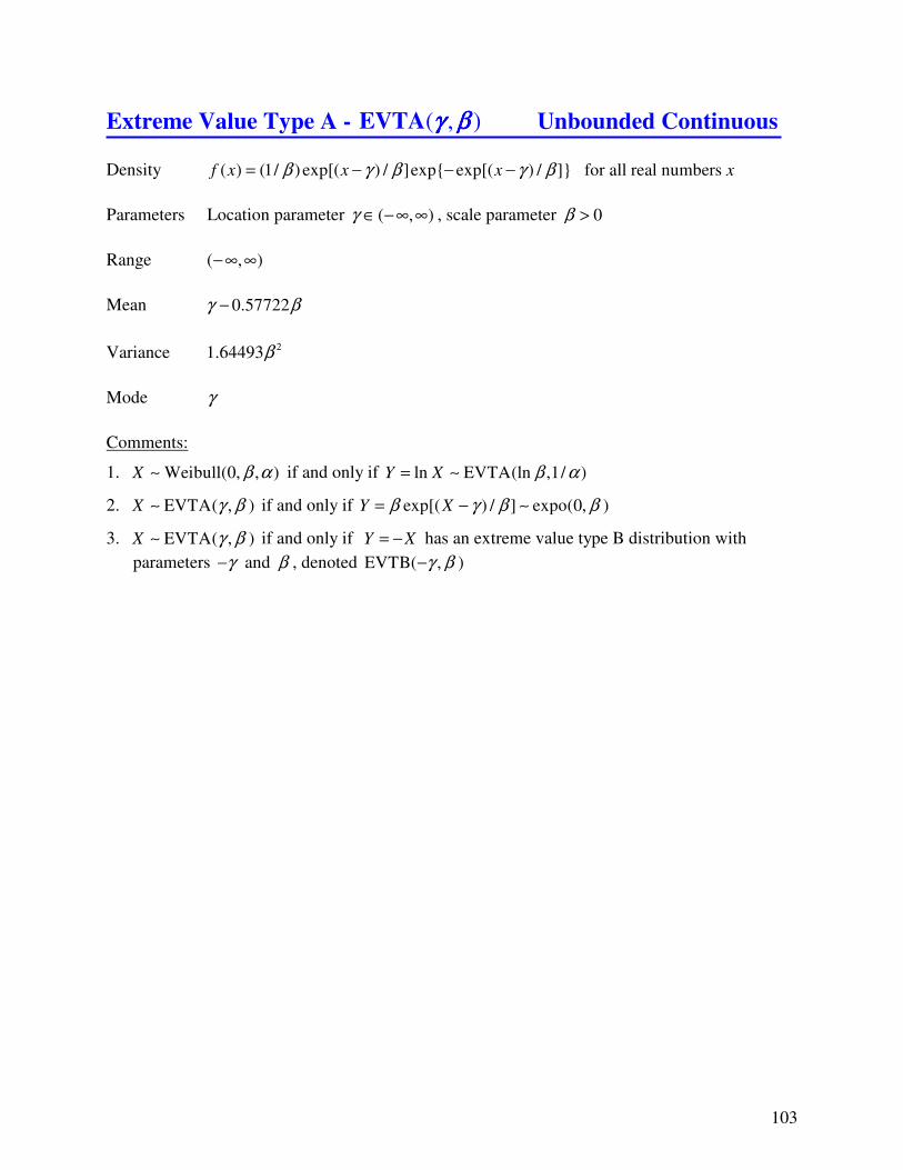
EVTA(γ, β)
EVTB(γ, β)
JSU(γ, β, α1,α2)
Laplace(γ, β)
logistic(γ, β)
N(γ, β)
t(ν)
96
100
102
103
104
112
113
115
120
128
91
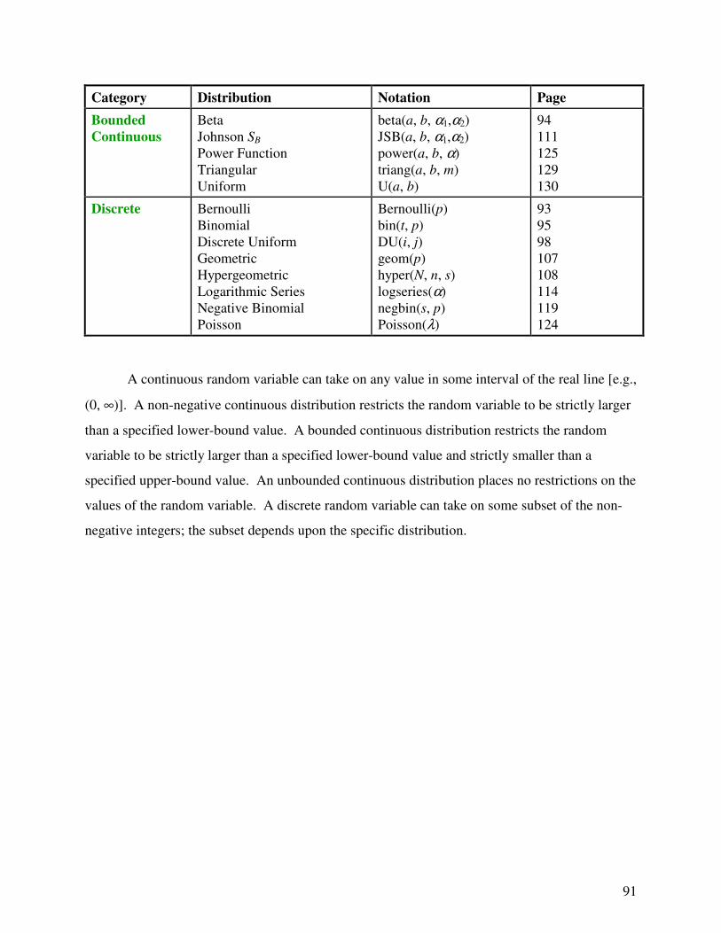
A continuous random variable can take on any value in some interval of the real line [e.g.,
(0, ∞)]. A non-negative continuous distribution restricts the random variable to be strictly larger
than a specified lower-bound value. A bounded continuous distribution restricts the random
variable to be strictly larger than a specified lower-bound value and strictly smaller than a
specified upper-bound value. An unbounded continuous distribution places no restrictions on the
values of the random variable. A discrete random variable can take on some subset of the non-
negative integers; the subset depends upon the specific distribution.
Category Distribution Notation Page
Bounded
Continuous
Beta
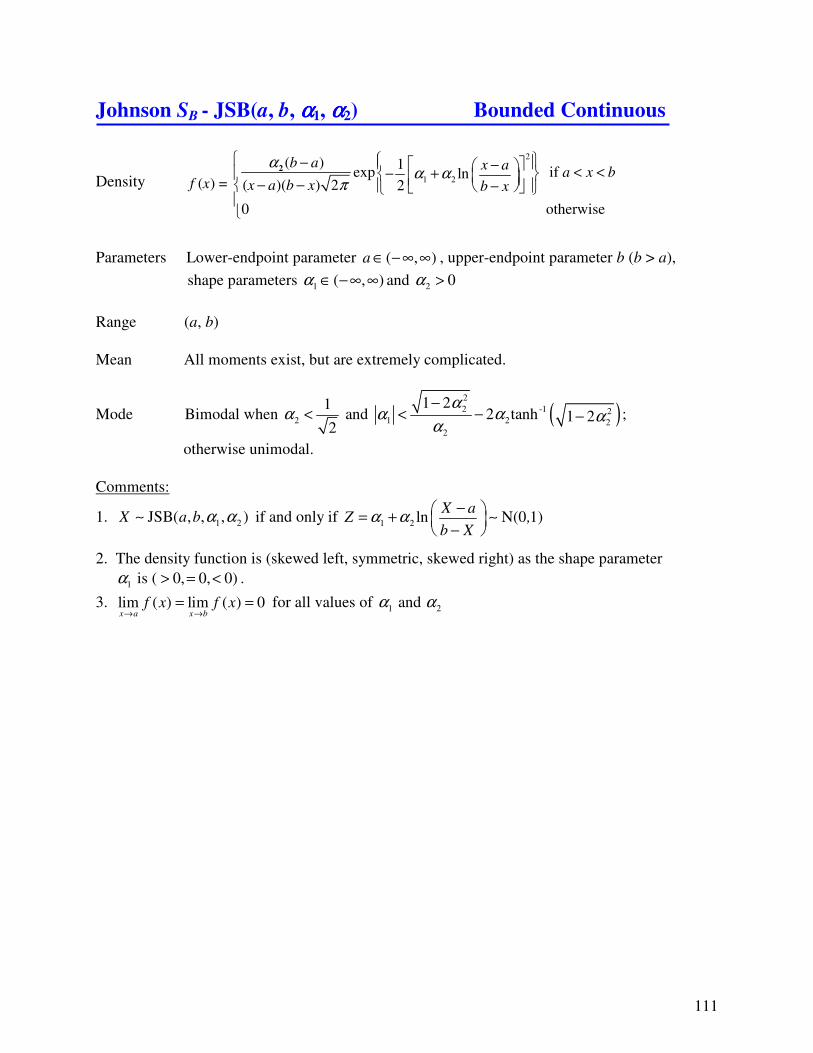
Johnson SB
Power Function
Triangular
Uniform
beta(a, b, α1,α2)
JSB(a, b, α1,α2)
power(a, b, α)
triang(a, b, m)
U(a, b)
94
111
125
129
130
Discrete Bernoulli
Binomial
Discrete Uniform
Geometric
Hypergeometric
Logarithmic Series
Negative Binomial
Poisson
Bernoulli(p)
bin(t, p)
DU(i, j)
geom(p)
hyper(N, n, s)
logseries(α)
negbin(s, p)
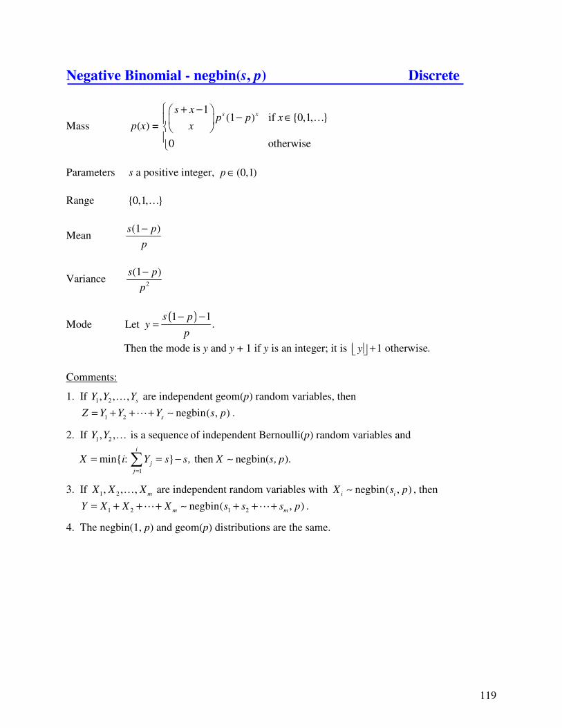
Poisson(λ)
93
95
98
107
108
114
119
124
92
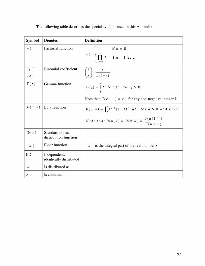
The following table describes the special symbols used in this Appendix:
Symbol Denotes Definition
!n Factorial function
1
1 i f 0
! i f 1, 2 ,
=
=
= = …
∏
n
k
n
nk n
t
x
Binomial coefficient !
!( )!
=
−
t t
x x t x
( )Γ z Gamma function 1
0
( ) fo r 0
∞
− −Γ = >∫z tz t e d t z
Note that ( 1) !Γ + =k k for any non-negative integer k.
( , )B u v
Beta function 11 1
0( , ) (1 ) fo r 0 a n d 0− −= − > >∫
u vB u v t t d t u v
( ) ( )N o te th a t ( , ) ( , )
( )
Γ Γ= =
Γ +
u vB u v B v u
u v.
( )Φ z Standard normal
distribution function
x Floor function x is the integral part of the real number x
IID Independent,
identically distributed
∼ Is distributed as
∈ Is contained in
93
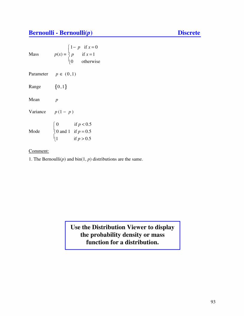
Bernoulli - Bernoulli(p) Discrete
Mass
1 if 0
( ) = if 1
0 otherwise
p x
p x p x
− =
=
Parameter ( 0 ,1)p ∈
Range { }0 ,1
Mean p
Variance (1 )p p−
Mode
0 if 0.5
0 and 1 if 0.5
1 if 0.5
p
p
p
<
= >
Comment:
1. The Bernoulli(p) and bin(1, p) distributions are the same.
Use the Distribution Viewer to display
the probability density or mass
function for a distribution.
94
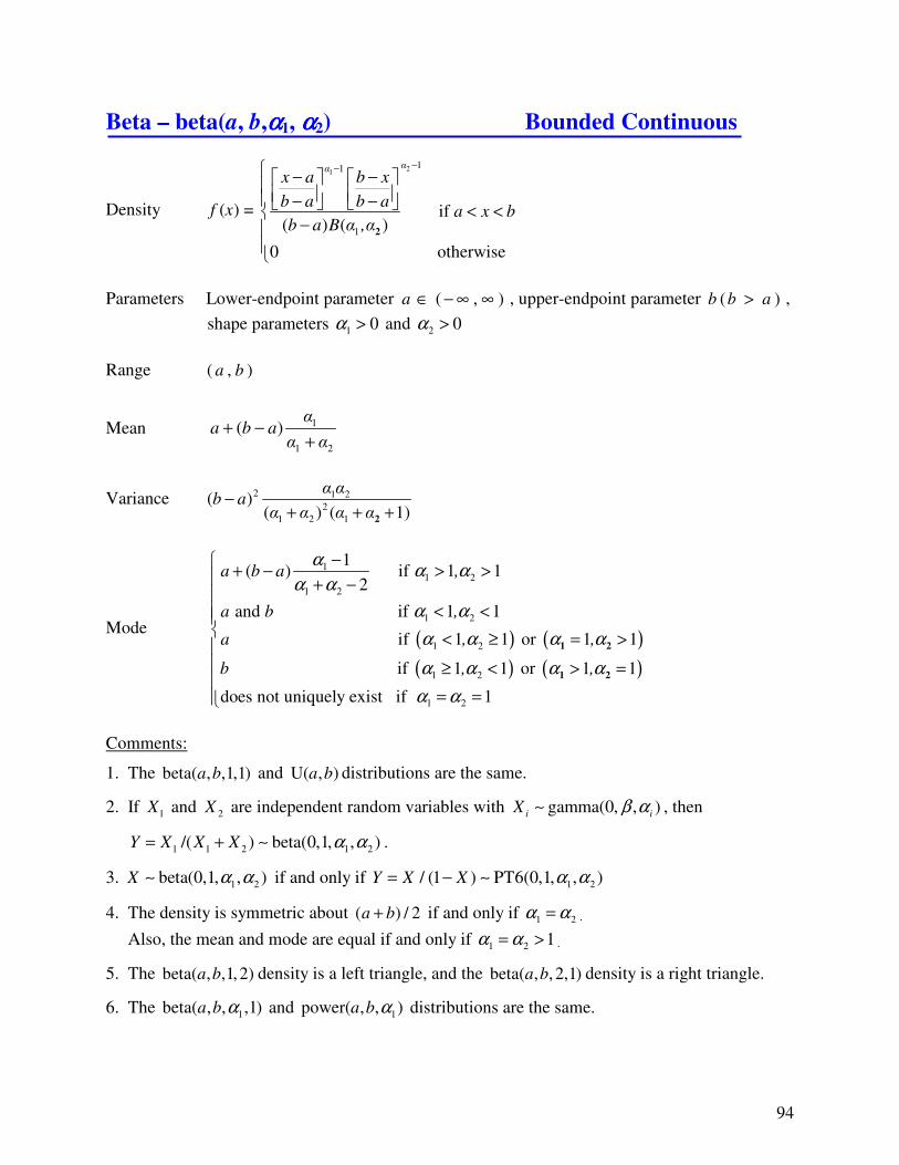
Beta – beta(a, b,αααα1, αααα2) Bounded Continuous
Density
21
11
1
( ) = if ( ) ( )
0 otherwise
2
−− − − − − < <−
ααx a b x
b a b af x a x b
b a B α ,α
Parameters Lower-endpoint parameter ( , )a ∈ − ∞ ∞ , upper-endpoint parameter ( )b b a> ,
shape parameters 1 0α > and 2 0α >
Range ( , )a b
Mean 1
1 2
( )α
a b aα α
+ −+
Variance 2 1 2
2
1 2 1
( )( ) ( 1)
α αb a
α α α α−
+ + +2
Mode ( ) ( )
( )
11 2
1 2
1 2
1 2
1 2
1( ) if 1 1
2
and if 1 1
if or 1 1 1 1
if o1 1
a b a ,
a b ,
a , ,
b ,
αα α
α α
α α
α α α α
α α
−+ − > >
+ −
< <
< ≥ = >
≥ <
1 2
( )
1 2
r 1 1
does not uniquely exist if 1
,α α
α α
> =
= =
1 2
Comments:
1. The beta( , ,1,1)a b and U( , )a b distributions are the same.
2. If 1X and 2X are independent random variables with gamma(0, , )i i
X β α∼ , then
1 1 2 1 2/( ) beta(0,1, , )Y X X X α α= + ∼ .
3. 1 2beta(0,1, , )X α α∼ if and only if 1 2/ (1 ) PT6(0,1, , )Y X X α α= − ∼
4. The density is symmetric about ( ) / 2a b+ if and only if 1 2α α= .
Also, the mean and mode are equal if and only if 1 2 1α α= > .
5. The beta( , ,1, 2)a b density is a left triangle, and the beta( , , 2,1)a b density is a right triangle.
6. The 1beta( , , ,1)a b α and 1power( , , )a b α distributions are the same.
95
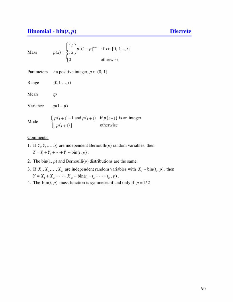
Binomial - bin(t, p) Discrete
Mass (1 ) if {0 1 }
( ) =
0 otherwise
x t xt
p p x , ,...,tp x x
−
− ∈
Parameters t a positive integer, p ∈ (0, 1)
Range {0,1, , )t…
Mean tp
Variance (1 )tp p−
Mode ( ) ( ) ( )
( )
1 and if is an integer1 1 1
otherwise1
p p pt t t
p t
− + + + +
Comments:
1. If 1 2, , ,t
Y Y Y… are independent Bernoulli(p) random variables, then
1 2 bin( , )t
Z Y Y Y t p= + + + ∼� .
2. The bin(1, p) and Bernoulli(p) distributions are the same.
3. If 1 2, , ,m
X X X… are independent random variables with bin( , )i i
X t p∼ , then
1 2 1 2bin( , )m m
Y X X X t t t p= + + + ∼ + + +� � .
4. The bin( , )t p mass function is symmetric if and only if 1/ 2p = .