USING LINEAR REGRESSION AND MIXED MODELS TO PREDICT HEALTH CARE COSTS AFTER AN INPATIENT EVENT by Christopher W Freyder BS in Industrial Math and Statistics, West Virginia University, 2014 Submitted to the Graduate Faculty of Graduate School of Public Health in partial fulfillment of the requirements for the degree of Master of Science University of Pittsburgh 2016
Transcript
USING LINEAR REGRESSION AND MIXED MODELS TO PREDICT HEALTH CARE COSTS AFTER AN INPATIENT EVENT
by
Christopher W Freyder
BS in Industrial Math and Statistics, West Virginia University, 2014
Submitted to the Graduate Faculty of
Graduate School of Public Health in partial fulfillment
of the requirements for the degree of
Master of Science
University of Pittsburgh
2016
ii
UNIVERSITY OF PITTSBURGH
Graduate School of Public Health
This thesis was presented
by
Christopher W Freyder
It was defended on
June 1, 2016
and approved by
Jeanine Buchanich, PhD, Research Assistant Professor, Department of Biostatistics, Graduate School of Public Health, University of Pittsburgh
Ada O. Youk, PhD, Associate Professor, Department of Biostatistics, Graduate School of
Public Health, University of Pittsburgh
Thesis Advisor: Eleanor Feingold, PhD, Senior Associate Dean, Professor, Department of Human Genetics, Graduate School of Public Health , University of Pittsburgh
Figure 1: Common covariance structures used in mixed models
9
4.0 METHODS
The purpose of this study was to estimate a formula that Gateway Health Plan® could use to
compare the average monthly cost in the six months before an inpatient event to the average
monthly cost six months after an inpatient event. This measure allows for a two month grace
period after the inpatient event, which was excluded from the calculations for the individual to
regain normal health. Therefore the six months used to calculate the average monthly cost after
the inpatient stay started 60 days after the last day of the inpatient stay. Gateway was interested
in a formula that could be used so when a new member comes to Gateway after an inpatient
event, they could estimate the cost based on the patient costs before the inpatient event. Both a
linear regression and a mixed model regression are reported and compared. For this analysis only
the data for Medicaid in PA was used because members in different states and who have
different coverage behave differently
Gateway’s initial attempt at solving this problem was to divide the average monthly cost
after an inpatient event by the average monthly cost before that event. While this gave them a
ratio for before and after costs, it did not take into account differences related to other
measureable factors, i.e. covariates. Therefore, we decided that a model was needed to achieve a
better estimate of the cost difference. Initially I ran a linear regression. Next, I log transformed
the outcome variable because it was heavily skewed. There were almost 3000 patients with no
claims in the outcome period. Because these values were undefined when the log transformation
10
was applied, I added $1 to all zero amounts before applying the log transformation. Because the
results were very similar to the linear regression, and because Gateway wanted a “simple”
model, we decided not to report the model with the log transformation. Lastly because the data
were “patient as their own control” measurements, I decided to run a mixed model as well to
allow the correlation between measurements to be handled.
4.1 DATA
Gateway data is stored in SQL databases. In order to extract the data, first I created a table in
SQL that contained anyone that had an inpatient event since January 1st, 2013. Then, I deleted
anyone who was not a member for at least 6 months before and 8 months after the date of their
inpatient event. These individuals had to be removed because if they did not have data for those
14 months, they would not have enough data to contribute to the study. Then I used the member
numbers of these individuals to pull any claims they had from 6 months before to 8 months after
the date of their inpatient stay. I also pulled age, race, and gender for these individuals. At this
point I moved the data to SAS using proc SQL to carry out further data manipulation.
Once the data were in SAS, anyone with more than one inpatient event was dropped, and
I calculated the total costs in the six months before and the six months after a two month grace
period. Individuals with more than one inpatient event were dropped because inpatient events are
the most expensive type, and the members with more than one significantly change the results.
The final dataset contained the variables member ID, average monthly cost before, average
monthly cost after, gender, race, and age. For the mixed model portion I had to manipulate the
11
data set so that the before and after costs were in one column with a time and patient identifier
for each measurement.
After talking to an expert on these types of events, patients who were under the age of 18,
over the age of 65, or who had inpatient events due to pregnancy were then removed from the
dataset. Patients under the age of 18 were removed because children are known to behave
differently than adults when it comes to insurance costs. Patients over the age of 65 were
removed because once a member turns 65 they become eligible for Medicare, and their Medicaid
benefits change. Patients whose inpatient stay was due to pregnancy were removed because
pregnancy is different than other inpatient stays. In the six months before giving birth an
individual will likely have many appointments and checkups, whereas for the time after a
pregnancy, most checkups are filed under the child’s insurance. This would likely be a different
behavior than most other inpatient events.
4.2 ANALYSIS PLAN
Once the dataset was finalized, I first ran descriptive statistics on the variables that were used to
create the models. I calculated the medians and interquartile range of average cost before,
average cost after, and age, as well as how they varied between the genders. I also calculated the
count of males and females and races in the data. I plotted a histogram of the ages in order to
look at the age distribution of the data. Reason for hospitalization was also looked at but most
code numbers had less than 5 observations, so it was omitted from the regressions.
After the descriptive statistics were analyzed, I used SAS to create linear regression
models. Average monthly cost after the inpatient event was the outcome variable, and I used
12
combinations of age, gender, race, and average monthly cost before as predictors. Because the
main purpose of this analysis was to see how cost before affected cost after, the average monthly
cost before variable was forced into the model. I used backwards selection to create a model of
the significant predictors. Then all combinations of models were run with those predictors, and
the models were compared using AIC and R2 criteria. For AIC, lower values are better, and
values within 2 of each other show there is no difference between the models. For R2 the model
with the higher value is considered to be a better fit, however, as covariates are added the R2 will
go up which must be taken into consideration when comparing models. The best fit regression
line, based on these criteria, can then be used as the formula for predicting average monthly costs
of a member after an inpatient event. I then calculated residuals to asses model fit on the final
chosen model.
Next I reshaped the data so that I could run a mixed model. This allowed me to have two
values of cost for each individual, one associated with before the IP, one after the IP. For this
model, I used cost as the outcome; time, gender, race, and age were the fixed effects, and patient
subject number was used as the random effect to allow for a random slope in the model and to
allow the correlation within patient measurements to be addressed. A random intercept was also
used in this model to allow for difference in patients baseline cost. For the mixed model I used
backwards elimination on the fixed effects to get to a final model. I chose to use variance
components as the correlation structure for this analysis. Studentized conditional residuals were
calculated and plotted in order to asses model fit of the final model.
After running these calculations, I decided to run a second set of models that would take
out individuals who had extreme costs in one time period but not the other. I decided to look at a
histogram of the difference in costs and to pick cutoffs that contained most of the data. This
13
method was chosen because it would eliminate some special cases that are not like the average
healthcare member. For example, some members might not go see a doctor until they have an
inpatient event, meaning even if they were sick and should have sought out care, their cost before
the event would be $0 and if the patient needs regular medical attention because of the event it
could result in high discrepancy of costs. Also this would eliminate individuals who had some
major cost before or after the event that is an unusual occurrence that greatly skewed their cost
for one period. After I used this method to delete members who I considered “outliers” the same
methods stated above were repeated to come up with an addition linear regression model and an
additional mixed model.
14
5.0 RESULTS
5.1 DESCRIPTIVE STATISTICS
Initially, 21811 patients were included. After I finalized the dataset by removing individuals who
did not fit the inclusion criteria, I was left with 17320 patients aged 18 to 65, who had one
inpatient event in the last three years not related to pregnancy, and were also a member of
Gateway Health Plan® for six month before and eight months after their inpatient event. Then
after looking at the difference between the before and after costs, I decided that a cutoff of ±
$30,000 would be used to get rid of outliers and create the second dataset, of 17214 members.
The median and IQR of average monthly cost before, average monthly cost after, and age for all
patients and stratified by gender are displayed in Table 1 for the whole dataset and Table 2 for
the subset of data where outliers were taken out of the sample.
Table 1: Descriptive Statisitcs for all patients
Variable Median (IQR)
Total n=17320 Male n=3938 Female n=13382
Average Monthly Cost Before ($) 277.67 (396.70) 197.91 (491.85) 291.53 (366.74)
Average Monthly Cost After ($) 104.96 (329.74) 189.35 (541.05) 87.80 (275.67)
Age (Years) 35.0 (25.5) 35.8 (25.6) 34.9 (25.5)
15
Table 2: Descriptive Statistics for data excluding outliers
Variable Median (IQR)
Total n=17214 Male n=3887 Female n=13327
Average Monthly Cost Before ($) 276.33 (392.17) 193.60 (478.51) 290.90 (363.38)
Average Monthly Cost After ($) 103.53 (323.70) 183.29 (521.44) 87.18 (273.628)
Age (Years) 35.0 (25.5) 35.8 (25.7) 34.8 (25.5)
As seen in Table 1 and Table 2, there is a difference in costs between males and females, and
also a difference in before/after costs. The median average monthly cost for males only goes
down about $10 a month (if the mean is looked at the cost actually goes up) but for females the
cost goes down over $200 per month. The larger IQR in the male categories can be explained by
the small sample size for men compared to women in this data. The cost is also much higher in
the female before cost but much lower in the female after cost compared too males. These results
led to inclusion of an interaction term between gender and time in the mixed model building
process.
Women account for about 78% of the individuals in this study. Women are known to be
more likely to qualify for Medicaid; however, this is still an extremely large difference. 51 men
and 55 females were dropped when the outliers were removed. Because there were so many
more females than males in this study, proportionally more men were removed.
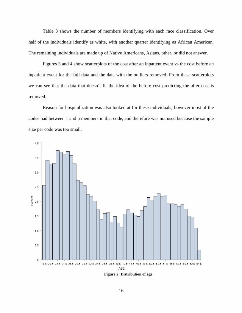
In figure 2, the distribution of ages can be seen. There is a bimodal distribution: a spike
in individuals between the ages of 20-30 as well as a smaller spike with individuals between the
ages of 49-55.
16
Table 3 shows the number of members identifying with each race classification. Over
half of the individuals identify as white, with another quarter identifying as African American.
The remaining individuals are made up of Native Americans, Asians, other, or did not answer.
Figures 3 and 4 show scatterplots of the cost after an inpatient event vs the cost before an
inpatient event for the full data and the data with the outliers removed. From these scatterplots
we can see that the data that doesn’t fit the idea of the before cost predicting the after cost is
removed.
Reason for hospitalization was also looked at for these individuals; however most of the
codes had between 1 and 5 members in that code, and therefore was not used because the sample
size per code was too small.
Figure 2: Distribution of age
17
Table 3: Self-Identified Race Counts
Race Frequency Percentage (%)
Native American 48 0.3
African American 4087 23.6
Asian 206 1.2
White 10870 62.8
Other 1826 10.5
Unknown 284 1.6
18
Figure 3: Scatterplot of after cost vs before cost for full data
Figure 4: Scatterplot of after cost vs before cost for data without outliers
19
5.2 LINEAR REGRESSION
The outcome variable for the linear regression was average monthly cost after the inpatient
event. Possible predictors were in this model included gender, age, race, and average monthly
cost before the inpatient event. First I ran linear regression model with all of the variables, and
race was seen to be not statistically significant (p-value =.3517) so it was removed. The, because
age and gender were significant, models with just age, just gender, and both were run, and AIC
and R2 values were calculated to see which model was the best fit. As seen by table 4, model 2
and model 4 have AIC’s that are less than 2 apart as well as the same R2 value. These models
also have the lowest AIC’s and the highest R2, so I concluded that these models are the best two
models, and there is no evidence that one model is better than the other. The model with just cost
before and gender was chosen since it will be a simpler model than the full model, yet just as
effective. After the final model was selected, studentized residuals were calculated, plotted and
can be seen in figures 5 and 6. In figure 5, it is seen that the homoscedasticity assumption is
violated. In figure 6 it is seen that the normality assumption is violated. The final model looks as
follows;
Average Cost After = 254.41+ 0.703 * Average Cost Before – 252.26 * Female
20
Table 4: Linear regression model comparisons for full dataset
Model Covariates AIC R2
1 Cost Before 240640.79 .507
2 Cost Before + Female 240463.19 .513
3 Cost Before + Age 240642.78 .507
4 Cost Before + Age + Female 240465.11 .513
Figure 5: Residual vs fitted for model 2
21
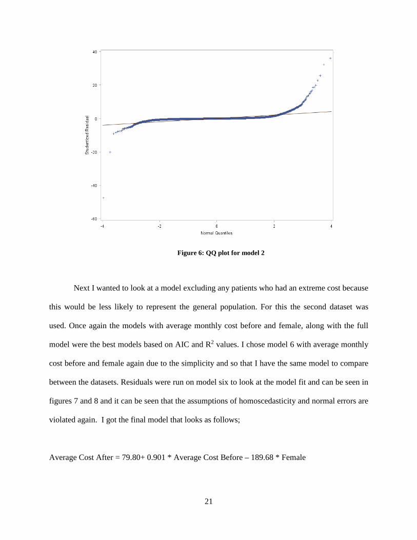
Figure 6: QQ plot for model 2
Next I wanted to look at a model excluding any patients who had an extreme cost because
this would be less likely to represent the general population. For this the second dataset was
used. Once again the models with average monthly cost before and female, along with the full
model were the best models based on AIC and R2 values. I chose model 6 with average monthly
cost before and female again due to the simplicity and so that I have the same model to compare
between the datasets. Residuals were run on model six to look at the model fit and can be seen in
figures 7 and 8 and it can be seen that the assumptions of homoscedasticity and normal errors are
violated again. I got the final model that looks as follows;
Average Cost After = 79.80+ 0.901 * Average Cost Before – 189.68 * Female
22
Table 5: Linear regression model comparisons for dataset without outliers
Model Covariates AIC R2
5 Cost Before 278655.10 .771
6 Cost Before + Female 278290.254 .776
7 Cost Before + Age 278654.81 .771
8 Cost Before + Female+ Age 278290.62 .776
Figure 7: Residuals vs fitted for model 6
23
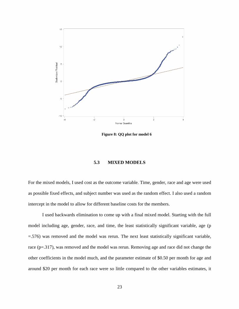
Figure 8: QQ plot for model 6
5.3 MIXED MODELS
For the mixed models, I used cost as the outcome variable. Time, gender, race and age were used
as possible fixed effects, and subject number was used as the random effect. I also used a random
intercept in the model to allow for different baseline costs for the members.
I used backwards elimination to come up with a final mixed model. Starting with the full
model including age, gender, race, and time, the least statistically significant variable, age (p
=.576) was removed and the model was rerun. The next least statistically significant variable,
race (p=.317), was removed and the model was rerun. Removing age and race did not change the
other coefficients in the model much, and the parameter estimate of $0.50 per month for age and
around $20 per month for each race were so little compared to the other variables estimates, it
24
was decided that age and race could safely be removed. I then added a time*gender interaction
because the descriptive statistics showed that there was a large difference in the genders. The
interaction term was statistically significant so it was kept in the model. The results from this
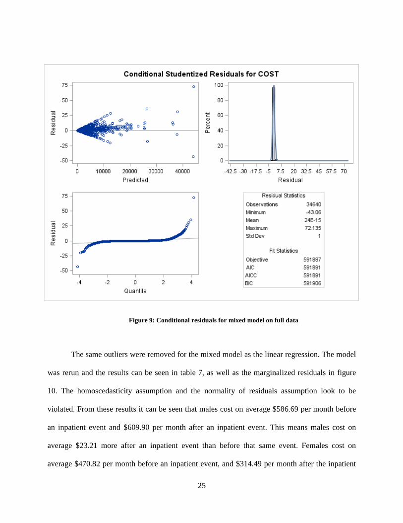
model can be seen in table 6. Marginalized residuals for the model were also calculated and can
be seen in figure 9. From these residuals it can be see that the homoscedasticity assumption as
well as the normality of errors assumption are both violated.
From this model I can get our estimates for the price difference of average monthly cost
before and average monthly cost after for each gender. For males the average monthly cost in the
six months before an inpatient event was $678.19, and the cost per month for the six months
after the inpatient event was $722.02. This shows that men cost an average of $43.83 per month
more after an inpatient event as before the inpatient event. For females the average monthly cost
before the inpatient event was $499.63 while the cost after the inpatient event was 344.48. This
yields that after an inpatient event females cost an average of $155.15 less per month than they
cost before the event.
Table 6: Coefficients and p-values of variables in full data mixed model
Variable Coefficient P-value
Time 43.83 0.0146
Female -178.56 <.0001
Time*Female -198.98 <.0001
Intercept 678.19 <.0001
25
Figure 9: Conditional residuals for mixed model on full data
The same outliers were removed for the mixed model as the linear regression. The model
was rerun and the results can be seen in table 7, as well as the marginalized residuals in figure
10. The homoscedasticity assumption and the normality of residuals assumption look to be
violated. From these results it can be seen that males cost on average $586.69 per month before
an inpatient event and $609.90 per month after an inpatient event. This means males cost on
average $23.21 more after an inpatient event than before that same event. Females cost on
average $470.82 per month before an inpatient event, and $314.49 per month after the inpatient
26
stay. Therefore, women cost on average $156.33 less per month after the inpatient event
compared to before the event.
Table 7: Coefficients and p-values of variables in the subset of data mixed model
Figure 10: Conditional residuals for mixed model without outliers
Variable Coefficient P-value
Time 23.21 0.0086
Female -115.87 <.0001
Time*Female -179.54 <.0001
Intercept 586.69 <.0001
27
6.0 DISCUSSION
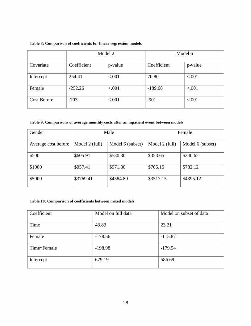
It can be seen from the linear regression equations that after deleting 106 of the extreme
observations, there is a substantial change in the coefficients. This change in coefficients greatly
affects how much gateway can expect to pay in certain situations. The comparison of coefficients
can be seen in table 8.
Table 9 shows the different payments Gateway can expect for patients with different
costs before the inpatient. Looking at the different starting costs, the comparison between the end
cost changes substantially between the models. Model 2 has higher expected costs for lower
initial costs, however model 6 has higher expected costs when the initial cost is higher. This can
be explained looking at the comparison of coefficients in table 8.
Because the members who were deleted were individuals with high costs in one time
period can explain the change in models. The members with the high cost after the event would
be outliers in the Y, and when removed would shift the whole regression line up, explaining the
larger intercept in model 2. The members with high cost before would be outliers in the X, and
would flatten the line out explaining the lower coefficient associated with cost before covariate
when removed.
28
Table 8: Comparison of coefficients for linear regression models
Model 2 Model 6
Covariate Coefficient p-value Coefficient p-value
Intercept 254.41 <.001 70.80 <.001
Female -252.26 <.001 -189.68 <.001
Cost Before .703 <.001 .901 <.001
Table 9: Comparisons of average monthly costs after an inpatient event between models
Gender Male Female
Average cost before Model 2 (full) Model 6 (subset) Model 2 (full) Model 6 (subset)
$500 $605.91 $530.30 $353.65 $340.62
$1000 $957.41 $971.80 $705.15 $782.12
$5000 $3769.41 $4584.80 $3517.15 $4395.12
Table 10: Comparison of coefficients between mixed models
Coefficient Model on full data Model on subset of data
Time 43.83 23.21
Female -178.56 -115.87
Time*Female -198.98 -179.54
Intercept 679.19 586.69
29
When looking at the mixed models the fixed effect coefficients, as seen in table 10, the
estimated parameters sizes are larger in the model on the full data than in the model on the data
without the outliers. This is easily explained by the fact that member with extremely high costs
were deleted. Deleting the high costs led to the model shifting down.
In the mixed models it can be seen that the time variable and the time female interaction
are significant for both models. This is important because it tells us that there is a difference in
before and after costs. However, looking at the parameter estimate, the interaction has a much
larger estimate than the time variable. This was expected when looking at the summary statistics
and the difference in the costs related to the genders. Because men did not change cost much, the
time variable does not have a large coefficient, but the interaction term have large coefficients
because females cost changes more between the different time points.
The results in this paper show that the cost before an inpatient event can be used as a
significant predictor of cost after an inpatient event. It also agrees with previous literature by
showing that males cost more individually than females, however females make up more of the
overall costs due to the high percentage of members being females. [11]
I would advise Gateway Health Plan® to use the mixed model on the subset of the data.
This model allows them to take into account correlation involved in a “patient as their own
control” study. I believe the subset of data are more appropriate to use since very few
individuals (0.6%) have extreme costs in one time period but not in the other.
30
6.1 LIMITATIONS
One possible problem with using these models is the range of values the outcome variable can
have depending on the inputs. In model 2 the intercept is larger than the estimated female
parameter; therefore there would never be a negative prediction for monthly cost after. For
model 6 however, it can be seen that the estimated female parameter is much larger than the
intercept, making it possible to obtain a negative value. Solving the equation for total after cost
of $0, any female with an average monthly cost before that is less than $121.95 will have an
expected monthly cost after of less than $0. Because the goal was to use this model to predict an
after cost, one option would be to assume that patients with a before cost less than this will just
have an average monthly cost after the inpatient event of $0, however this is not practical and a
solution to this problem should be found.
Another problem with these models can be seen when looking at the residual plots. In
both models it can be seen that there is a violation of the homoscedasticity assumption. There is a
pattern of the magnitude of the maximum negative residuals being proportional to the predicted
value. However, once the values get larger, the variances seem to be more equal. In the QQ plots,
the residuals look to have a heavy tailed distribution rather than a normal distribution. This
means that the normality of residuals assumption is also violated.
Looking at the residuals for the mixed models, the conditional residuals will be used.
These residuals are the difference between the observed and fitted values. These residuals take
into account the known information in the random variable. [9] From the residual panels, it can
be seen in the model run on the full dataset, that there is a clear fanning pattern throughout
predicted values, violating the heteroscedasticity assumption. The QQ plot for this model shows
that the residuals are once again heavy tailed.
31
In the model run on subset of the data, like with the linear regression, the residuals have a
fanning pattern at the beginning but even off as the predicted values get higher. The QQ plot
associated with this model shows that the normality of the residuals are violated. With all of the
bad diagnostics, none of these models seem to be a good fit. Therefore when using any of these
models, results should only be provisionary.
6.2 FUTURE DIRECTIONS
The next step with the models developed in this paper would be to use other available data to
validate the models. Gateway has data from other states that could be used to validate the models
I developed. Gateway could also look at incoming patients and track their costs in the future to
see how the model works at predicting in the intended situation.
While this model can be used to predict costs of patients who had an inpatient event, the
lack of model fit is concerning. There are many possibilities that could contribute to finding a
better model. First, other regression methods should be considered in order to address the
specific difficulties that these models have in fitting the given data. Possible solutions would be
polynomial models, tobit models, or other models that are nonparametric.
Another solution could be transforming the data. Because the nature of healthcare costs
are skewed, transformations can be run on the cost variable to see if a better model fit can be
obtained. Also, other covariates could be considered. The difference in gender may be due to
some other confounding variable. I would like to investigate the reason for hospitalization in
order to see if the genders are equally represented in each code. I believe that different reasons
for hospitalization could explain the cost discrepancy between genders. Because there are so
32
many hospitalization codes that have few observations, they would need to be grouped by similar
codes to run this analysis.
Along with reason for hospitalization, I would like to look into the comorbidity loads of
the individuals in this study. This could be another confounder for the interaction term. The
number of comorbidities an individual can change, so I could look at the average comorbidities
before and after the inpatient event by gender. Even if this term doesn’t contribute to the
interaction, it could be statistically significant in predicting costs.
Similarly to the problem seen with reason for hospitalization, I saw that race had most
individuals grouped into White or African American and not many individuals in the other four
categories. I would like to collapse the race categories to White, African American, or other and
rerun the analysis to see if anything would change.
Another possibility to consider while moving forward is that we want to consider the
average healthcare member for these predictions. Since most individuals have relatively low
cost, I could also fit a model on just members with costs less than a certain amount. This would
allow us to have another model to be used on individuals who come into Gateway with a low
cost before an inpatient event.
There are still a lot of possibilities to be considered for this type of analysis. While this
paper explored some solutions to cost analysis in healthcare, I believe this problem needs to be
analyzed more in order to come up with a better way to estimate health care costs for members
after they have an inpatient event.
33
6.3 PUBLIC HEALTH SIGNIFICANCE
This research will help Gateway Health Plan® to evaluate research interventions to assess
whether they lower health care costs. Being able to evaluate if interventions are cost efficient
will improve healthcare leading to an improvement in population health.
34
BIBLIOGRAPHY
1. Ayanian, John Z. “The Costs of Racial Disparities in Health Care.” Harvard Business Review. N.p., 01 Oct. 2015. Web. 25 May 2016.
2. “Are you a Hospital Inpatient or Outpatient?” The Official U.S. Government Site for Medicare. Medicare.gov, n.d. Web. 25 Apr. 2016.
3. Brown H and Prescott. Applied Mixed Models in Medicine, 2nd edition. Chichester, England: John Wiley, 2006. Print
4. “How do Medicare Advantage Plans Work?” The Official U.S. Government Site for Medicare.
Medicare.gov, n.d. Web. 21 May 2016.
5. Littell, Ramon C., George A. Milliken, Walter W. Stroup, Russell D. Wolfinger, and Oliver Schabenberger. 2006. SAS® for Mixed Models, Second Edition. Cary, NC: SAS Institute Inc.
6. Mendelson, D. N., and W. B. Schwarts “The Effects of Aging and Population Growth on
Health Care Costs.” Health Affairs 12.1 (1993): 119-25. 7. Osborne, Jason. “Four Assumptions of Multiple Regression That Researchers Should Always
Test.” Practical Assessment, Research & Evaluation, 2002. Web. 14 Apr. 2016. 8. “Policy Basics: Introduction to Medicaid.” Center on Budget and Policy Priorities. N.p., 19
June 2015. Web. 13 Mar. 2016. 9. Schabenberger, O. (2004) Mixed Model Influence Diagnostics, SUGI 29 – Statistics and Data
Analysis, Paper 189- 29. 10. SAS Institute Inc., SAS 9.1.3 Help and Documentation, Cary, NC: SAS Institute Inc., 2002-
2004.
11. “U.S. Personal Health Care Spending by Age and Gender.” Centers for Medicare and Medicaid Services N.p., 2010. Web. 25 May 2016.
12. “What is Medicare?” The Official U.S. Government Site for Medicare. Medicare.gov, n.d.