Using Xplor–NIH for NMR molecular structure determination

Charles D. Schwieters a,*, John J. Kuszewski a, G. Marius Clore b,*

a Division of Computational Bioscience, Center for Information Technology, National Institutes of Health, Building 12A, Bethesda, MD 20892-5624, USAb Laboratory of Chemical Physics, National Institute of Diabetes and Digestive and Kidney Diseases, National Institutes of Health,

Building 5, Bethesda, MD 20892-0510, USA

Received 2 September 2005

Available online 20 December 2005

Keywords: Structure determination; NMR restraints; Optimization; Computational Toolbox; Proteins; Nucleic acids

Contents

1. Introduction . . . . . . . . . . . . . . . . . . . . . . . . . . . . . . . . . . . . . . . . . . . . . . . . . . . . . . . . . . . . . . . . . . . . . . . . . . . . . . . . . . . . 48

2. The Python interface . . . . . . . . . . . . . . . . . . . . . . . . . . . . . . . . . . . . . . . . . . . . . . . . . . . . . . . . . . . . . . . . . . . . . . . . . . . . . . 48

3. Potential energy terms . . . . . . . . . . . . . . . . . . . . . . . . . . . . . . . . . . . . . . . . . . . . . . . . . . . . . . . . . . . . . . . . . . . . . . . . . . . . . 49

3.1. Native Python potential terms . . . . . . . . . . . . . . . . . . . . . . . . . . . . . . . . . . . . . . . . . . . . . . . . . . . . . . . . . . . . . . . . . . 50

3.1.1. NOE distance restraint potential . . . . . . . . . . . . . . . . . . . . . . . . . . . . . . . . . . . . . . . . . . . . . . . . . . . . . . . . . . 50

3.1.2. RDC potential . . . . . . . . . . . . . . . . . . . . . . . . . . . . . . . . . . . . . . . . . . . . . . . . . . . . . . . . . . . . . . . . . . . . . . . 50

3.1.3. The CSA potential . . . . . . . . . . . . . . . . . . . . . . . . . . . . . . . . . . . . . . . . . . . . . . . . . . . . . . . . . . . . . . . . . . . . 51

3.1.4. J-coupling potential . . . . . . . . . . . . . . . . . . . . . . . . . . . . . . . . . . . . . . . . . . . . . . . . . . . . . . . . . . . . . . . . . . . 52

3.1.5. PotList—a collection of potential terms . . . . . . . . . . . . . . . . . . . . . . . . . . . . . . . . . . . . . . . . . . . . . . . . . . 52

3.2. XPLOR potential terms . . . . . . . . . . . . . . . . . . . . . . . . . . . . . . . . . . . . . . . . . . . . . . . . . . . . . . . . . . . . . . . . . . . . . . . 53

3.2.1. Non-bonded potential . . . . . . . . . . . . . . . . . . . . . . . . . . . . . . . . . . . . . . . . . . . . . . . . . . . . . . . . . . . . . . . . . . 53

3.2.2. Radius of gyration . . . . . . . . . . . . . . . . . . . . . . . . . . . . . . . . . . . . . . . . . . . . . . . . . . . . . . . . . . . . . . . . . . . . 53

3.2.3. Torsion angle database . . . . . . . . . . . . . . . . . . . . . . . . . . . . . . . . . . . . . . . . . . . . . . . . . . . . . . . . . . . . . . . . . 53

3.3. Other potential terms . . . . . . . . . . . . . . . . . . . . . . . . . . . . . . . . . . . . . . . . . . . . . . . . . . . . . . . . . . . . . . . . . . . . . . . . 54

3.4. Adding a new potential term . . . . . . . . . . . . . . . . . . . . . . . . . . . . . . . . . . . . . . . . . . . . . . . . . . . . . . . . . . . . . . . . . . . 54

4. Use of the Internal Variable Module (IVM) . . . . . . . . . . . . . . . . . . . . . . . . . . . . . . . . . . . . . . . . . . . . . . . . . . . . . . . . . . . . . 55

5. Parallel computation of structures . . . . . . . . . . . . . . . . . . . . . . . . . . . . . . . . . . . . . . . . . . . . . . . . . . . . . . . . . . . . . . . . . . . . 57

6. Ensemble refinement . . . . . . . . . . . . . . . . . . . . . . . . . . . . . . . . . . . . . . . . . . . . . . . . . . . . . . . . . . . . . . . . . . . . . . . . . . . . . . 57

6.1. Order parameters . . . . . . . . . . . . . . . . . . . . . . . . . . . . . . . . . . . . . . . . . . . . . . . . . . . . . . . . . . . . . . . . . . . . . . . . . . . 58

6.2. Crystallographic B-factors . . . . . . . . . . . . . . . . . . . . . . . . . . . . . . . . . . . . . . . . . . . . . . . . . . . . . . . . . . . . . . . . . . . . . 58

6.3. Shape term . . . . . . . . . . . . . . . . . . . . . . . . . . . . . . . . . . . . . . . . . . . . . . . . . . . . . . . . . . . . . . . . . . . . . . . . . . . . . . . . 58

6.4. Constraining relative atom position with RAPPot . . . . . . . . . . . . . . . . . . . . . . . . . . . . . . . . . . . . . . . . . . . . . . . . . . . 59

7. Other Xplor–NIH facilities . . . . . . . . . . . . . . . . . . . . . . . . . . . . . . . . . . . . . . . . . . . . . . . . . . . . . . . . . . . . . . . . . . . . . . . . . 59

7.1. Probabilistic NOE assignment algorithm for automated structure determination (PASD) . . . . . . . . . . . . . . . . . . . . . . . 59

7.2. VMD–XPLOR interface . . . . . . . . . . . . . . . . . . . . . . . . . . . . . . . . . . . . . . . . . . . . . . . . . . . . . . . . . . . . . . . . . . . . . . 59

7.3. Analysis and validation . . . . . . . . . . . . . . . . . . . . . . . . . . . . . . . . . . . . . . . . . . . . . . . . . . . . . . . . . . . . . . . . . . . . . . . 60

7.4. Test suite . . . . . . . . . . . . . . . . . . . . . . . . . . . . . . . . . . . . . . . . . . . . . . . . . . . . . . . . . . . . . . . . . . . . . . . . . . . . . . . . . 60

8. Conclusion . . . . . . . . . . . . . . . . . . . . . . . . . . . . . . . . . . . . . . . . . . . . . . . . . . . . . . . . . . . . . . . . . . . . . . . . . . . . . . . . . . . . . 60

Acknowledgements . . . . . . . . . . . . . . . . . . . . . . . . . . . . . . . . . . . . . . . . . . . . . . . . . . . . . . . . . . . . . . . . . . . . . . . . . . . . . . . 61

References . . . . . . . . . . . . . . . . . . . . . . . . . . . . . . . . . . . . . . . . . . . . . . . . . . . . . . . . . . . . . . . . . . . . . . . . . . . . . . . . . . . . . 61

Progress in Nuclear Magnetic Resonance Spectroscopy 48 (2006) 47–62

www.elsevier.com/locate/pnmrs

0079-6565/$ - see front matter Published by Elsevier B.V.

doi:10.1016/j.pnmrs.2005.10.001

* Corresponding authors.

E-mail addresses: charles.schwieters@nih.gov (C.D. Schwieters), mariusc@intra.niddk.nih.gov (G. Marius Clore).

C.D. Schwieters et al. / Progress in Nuclear Magnetic Resonance Spectroscopy 48 (2006) 47–6248

1. Introduction

Xplor–NIH [1] is a generalized package for biomolecular

structure determination from experimental NMR data com-

bined with known geometric data. This is achieved by seeking

the minimum of a target function comprising terms for the

experimental NMR restraints, covalent geometry and non-

bonded contacts using a variety of optimization procedures

including molecular dynamics in Cartesian and torsion angle

space, Monte Carlo methods and conventional gradient-based

minimization.

Xplor–NIH was originally derived from XPLOR [2] version

3.851 and contains all of the functionality therein. However,

Xplor–NIH incorporates numerous completely new features

designed to render its overall architecture highly flexible and to

foster the rapid and easy development of new and improved

functionality. This architecture is comprised of a framework

written in CCCwith user interfaces to the Python and Tclscripting

languages. Features introduced since XPLOR 3.851 include:

† A number of additional NMR-specific features related to

refinement against NMR observables [3–7] not included in

XPLOR 3.851, as well as a variety of knowledge-based

database potentials of mean force [8–10].

† A reduced variable dynamics module which permits com-

pletely generalized minimization and molecular dynamics in

torsion angle and Cartesian coordinate space, as well as the

effective treatment of rigid bodies [11].

† The PASD [12] facility for automatic NOE assignment and

structure determination directly from automatically peak-

picked multidimensional spectra.

† Facilities for refinement against an ensemble of structures, for

use, for example, in studies of dynamics [13,14].

† A direct interface to the VMD-XPLOR visualization package

[15].

We note that despite the numerous additions and modifications

present in Xplor–NIH, great care has been taken to ensure that old

XPLOR scripts still run as expected. CNS [16] scripts can also be

run with very minor modifications.

Xplor–NIH is written in a combination of languages. The

older code of the XPLOR interface is written in Fortran 77, and it

is still possible to compile just this code subset, corresponding

closely to XPLOR 3.851. One major change to the Fortran code

was the removal of all structure-based limits, so that the

maximum number of atom, bonds, etc. is now determined by

the amount of the computer’s RAM, and not by pre-compiled

constants. Most recent computationally intensive code has been

developed in the CCC language, with interfaces to the Python

and Tcl scripting languages generated automatically with the

SWIG package [17]. Much of the non-computationally intensive

code is now being developed directly in the Python and Tcl

languages, and thus is directly accessible for modification by the

end-user without recompilation. The Python interface to Xplor–

NIH in particular provides an extensible toolbox for developing

further functionality. The full source code package is available by

sending email to requests@nmr.cit.nih.gov. Binary packages for

most popular Unix and Unix-like operating systems (such as

Linux and Mac OS X), as well as documentation and support are

available directly from http://nmr.cit.nih.gov/Xplor–NIH/.

An agreement with the Accelrys corporation allows us to

distribute Xplor–NIH in its entirety (in both source and

executable formats) freely to academic users, as well as to

distribute freely to industrial users those portions of Xplor–NIH

not based on the legacy XPLOR Fortran framework. Commercial

use of Xplor–NIH should be arranged with the Accelrys

Corporation, but code developed outside the old XPLOR

framework (the CCC interface including the IVM, etc.) is

available to commercial and noncommercial entities.

Xplor–NIH is a collaborative effort, with groups worldwide

contributing advice and computer code. Additional contributions

are encouraged, and are advantageous to the contributors as well

as to end-users. New contributions should adhere to Xplor–NIH

coding conventions, and be accompanied by appropriate testing

scripts to assure reproducible future operation.

This review provides an overview of recent Xplor–NIH

development, and an introduction complete with example code,

via the Python interface. This review is organized as follows.

Section 2 presents a brief introduction to the Python interface.

Section 3 introduces some of the most often used potential terms

for NMR structure determination, along with Python example

code. Section 4 discusses the internal variable module used to

manipulate atomic coordinates. Section 5 introduces the parallel

structure calculation facilities, while Section 6 discusses facilities

for simultaneous refinement of ensembles of structures. Finally,

Section 7 presents brief overviews of other Xplor–NIH facilities.

2. The Python interface

There are three scripting interfaces to Xplor–NIH: the legacy

XPLOR interface of XPLOR 3.851 (which closely resembles that

of CNS [16]), and the Python and Tcl scripting interfaces. These

later two general purpose scripting languages provide a much more

general purpose modern programming environment than the

XPLOR interface. Having two modern interfaces also facilitates

better interaction with more external packages. Of these scripting

languages, the Python interface is the more well-developed, and

only Python code examples will be covered in this review. This

review does assume some familiarity with the Python language.

For a good introductory tutorial to Python see Ref. [18].

The Python interpreter is invoked via the xplor py or pyXplor

commands. In Xplor–NIH’s Python interface, functions and class

definitions are placed in module namespaces; a reference manual

for all Xplor–NIH modules is available from [19]. The Python

built-in function help can be used to get immediate help about

Python objects. The following conventions are used in Xplor–

NIH’s Python interface: module and function names start with

lower-case letters and class names start with upper-case letters.

Functions used to configure standard settings for dynamics,

minimization and XPLOR potential setup can be found in the

protocol module. For example, to load atom definitions and

covalent coordinate definitions from a protein structure file (PSF)

(which contains atom information and covalent geometry

definitions for a particular structure), the initStruct function

C.D. Schwieters et al. / Progress in Nuclear Magnetic Resonance Spectroscopy 48 (2006) 47–62 49

can be used as seen in Listing 1. Listing 1 also shows that PSF

information can also be directly generated from an amino acid

sequence using functions in the psfGen module.

Listing 1. Loading PSF information from file, or generating it from sequence.

protein.psf would contain a pre-calculated PSF file, while protein.

seq would contain a list of whitespace-separated 3-character residue names.

PSF information is required before executing any of the other code listed in this

review.

Global settings such as the random number seed and the error

logging level are accessed via the built-in simWorld object.

Access to arrays of atomic properties can be obtained via methods

of the simulation object in the built-in xplor module. More

convenient access and manipulation of atomic properties can be

obtained via AtomSel objects, as demonstrated in Listing 2. The

atom selection language is identical to that in the XPLOR

interface. Coordinates can be easily read and written via the

PDBTool class as seen in Listing 3.

Listing 2. Examples of manipulation of atom properties via AtomSel objects.

Listing 3. Using the PDBTool for reading and writing atomic coordinates. In

this example, an unregularized average structure is calculated and written to

file.

Listing 3 also demonstrates some of the basic linear algebra

functionality present in Xplor–NIH’s Python interface. More

information about this functionality is available in the

documentation for the cdsMatrix and cdsVectormodules.

3. Potential energy terms

Xplor–NIH potential terms can be divided into five general

classes:

† Those terms which reflect how well NMR observables

calculated from a molecular structure match their experimen-

tal counterparts. Examples include NOE and dipolar coupling

restraint terms.

† Those terms which enforce covalent geometry and prevent

bad atom-atom contacts, as determined from high-resolution

crystal structures. Example terms include bond, angle,

improper dihedral, and non-bonded terms.

† Potential terms of mean force derived from the Protein Data

Bank which bias structures towards existing features seen in

the database. Examples include the RAMA multi-dimensional

torsion angle database potential term [20,21]. When these

terms are designed, special care is taken so that they are

readily overridden by experimental restraints in cases of

conflict.

† Other potential terms used to aid with structure determination-

generally to aid with convergence or to enforce other physical

information gleaned about the structure. For example, such

terms include XPLOR’s NCS and HARM terms, which

enforces symmetry, and restrains atomic positions, respect-

ively.

† Potential terms to refine against X-ray crystallographic

observables [22–24]. These terms might be used to carry

out a joint NMR/X-ray structure determination [25].

Ideally, only the first class of potential terms would be

necessary in structure determination, but NMR restraints alone do

not contain sufficient structural information.

C.D. Schwieters et al. / Progress in Nuclear Magnetic Resonance Spectroscopy 48 (2006) 47–6250

3.1. Native Python potential terms

Potential terms coded in CCC and the corresponding SWIG-

generated Python wrapper objects have the following methods in

common:

potName()—type of potential term, e.g. NOEPot

instanceName()—name given by user script when object

is created

scale() setScale()—get and set the term’s scale

factor. This is generally 2 times the force constant

calcEnergy()—calculate and return the term’s energy

Listing 4. Creation and analysi

The native Python potentials are summarized below, complete

with example Python code illustrating creation and manipulation

of the terms.

3.1.1. NOE distance restraint potential

This term is an implementation of the standard NOE potential

which restrains distances to those derived from NOE cross-peak

intensities. Because of the qualitative nature of NOE distance

restraints, a piecewise quadratic potential (referred to as ‘square’)

is usually employed

VpQuadðx; xC; xKÞZ

ðxKxCÞ2 if xOCxC

ðxCxKÞ2 if x!KxK

0 otherwise:

;

8>><>>:

(1)

where xC and xK represent the upper and lower bounds of a flat

zero-valued region. The usual NOE energy term is

ENOE ZwNOEVpQuadðrNOEKrðObsÞNOE ; r

CNOE; r

KNOEÞ; (2)

where wNOE is the scale factor and the distances rNOE and rðObsÞNOE

are calculated from a given structure and derived from NOE

cross-peak intensities, respectively. NOEPot also supports a

potential form which is linear at large distances [26].

NOE assignments can involve more than two atoms, such that

rNOE is averaged in some fashion. For ambiguous NOE

assignments sum ‘averaging’ [27] is the most common method

for distance computation:

rNOE Z ðXi;j

jqiKqjjKaÞK1=a: (3)

where qi and qj are the the position of atoms i and j, the ij sum is

over all atom pairs associated with the given NOE cross-peak,

and aZ6 is usually used. The NOEPot term also supports the

center averaging method which uses the distance between the

centers of the two selections. This averaging method is

appropriate for use with methyl groups and with non-

stereospecifically assigned methylenes and aromatics when

used with a pseudo-atom correction [28]. This potential term

can read standard XPLOR NOE assignment tables. Listing 4

demonstrates creation and analysis of an NOEPot.

s of an NOE Potential term.

3.1.2. RDC potential

Residual dipolar couplings (RDCs) are calculated from a

structure as [29]:

dRDCcalc ZDa½ð3u

2zK1ÞC

3

2hðu2

xKu2y�; (4)

where ux, uy, uz are projections of bond vectors onto the principal

axes of an alignment tensor describing overall molecular

orientation, while Da and h are the associated axial and rhombic

tensor components. Thus, this observable depends on the

orientation of an inter-atomic vector relative to a molecule-

fixed axis. The global and quantitative nature of this restraint

make it complementary to NOE distance restraints in determining

accurate NMR structures [30,31]. A simple quadratic harmonic

potential is usually used with weighting factors as specified

below.

The Python-based RDC term encodes the complete

5-degrees of freedom alignment tensor in a VarTensorobject in which 4 atoms represent the orientation of the

tensor’s principal axes, and two additional atoms encode

the Da and h in values of the angles made with the axis

atoms as shown in Fig. 1. Thus, Da and h can be

optionally optimized along with tensor orientation. The

RDC potential supports reading both SANI- and DIPO-

style XPLOR restraint tables; however, the atom selections

of the axis atoms are ignored in these tables.

The RDCPot term allows ambiguous assignment for

averaging RDCs involving indistinguishable atoms,

allows ambiguous Da sign and can also optionally include the

C.D. Schwieters et al. / Progress in Nuclear Magnetic Resonance Spectroscopy 48 (2006) 47–62 51

1=r3 atom–atom distance dependence of dRDC—which

is important for measurements involving non-bonded atoms [4].

The values of the tensor can be calculated (by singular

value decomposition) from a given structure using the

calcTensor helper function from the varTensorToolsmodule. An example of setting up an RDCPot is shown in

Listing 5. Examples of experiments in different orienting

media and of multiple experiments within a single medium

are shown in Listing 6. This figure also demonstrates the

usual scaling convention used when more than one

experiment is included in the structure calculation.

Listing 5. Creating and manipulating RDCPot terms. The VarTensor object enc

Listing 6. Example of using multiple RDC experiments in the same and in differen

experiments relative to each other. The value of the scale energy scale factor reflec

3.1.3. The CSA potential

The tensor nature of the chemical shift can be gleaned by

measurement in a weakly orienting medium [5]. The chemical

shift anisotropy provides additional orientational information for

structure calculation [32,33]. The formula for calculating the

CSA of an atom is

dCSAcalc Z

Xab

Aasb cos2qab; (5)

where a and b range over the three principal axes of the

molecular alignment tensor, and the CSA tensor, respectively.

The principal moments of the orientation and CSA tensors are

represented by Aa and sb, respectively. qab is the angle between

principal axes a and b. A harmonic potential is typically used.

odes all information about the alignment tensor.

t orienting media. This example includes the usual convention for scaling the

ts that the error in the CAHA experiment is 3 times that of the NH_2 experiment.

X

Y

Z

P2

P1

φ2

θ1

Fig. 1. Axis parameter atoms for fully varying orientation axis. Four atoms

(X, Y, Z, and O) represent the orientation of the tensor principal axes, and

P1 and P2 are used to represent Da and h, respectively. The representation

of the tensor magnitude is DaZDamax cos q1, where Damax is the maximum

allowed value of Da and q1 is the axial angle between the projection of the

qP1KqO vector on the X–O–Y plane and the qXKqO vector, and takes

values between 0 and 2p. The rhombicity is calculated as hZ2=3 sin f2,

where f2 is the azimuthal angle between qZKqO and qP2KqO, and takes

values between 0 and p.

Listing 8. Setting up the J-coupling potential term. The Karplus coefficients can

alternatively be set using the COEF statement in the J-coupling assignment table.

C.D. Schwieters et al. / Progress in Nuclear Magnetic Resonance Spectroscopy 48 (2006) 47–6252

A CSAPot is created using the code shown in Listing 7. The

create_CSAPot helper function determines the atom type

involved and uses built-in values of the appropriate CSA tensor

parameters. Of course, it is possible to specify alternative values.

Note that multiple CSA orientation axis definitions are used; the

current implementation supports all of those introduced in Refs.

[5,32].

Listing 7. Setting up the CSA potential term. The default values of the CSA

tensor parameter values are configured in the csaPotTools module, and

these may easily be modified. The bTensor object is the VarTensor

defined in Listing 6.

Listing 9. Creation and manipu

3.1.4. J-coupling potential

Three-bond J coupling experiments provide quantitative

information about torsion angle values through the empirical

Karplus equation [34], calculated from a structure as:

J ZA cos2ðqCq*ÞCB cosðqCq*ÞCC; (6)

where q is the value of the torsion angle in question, q* is a

phase, and A, B, and C are Karplus coefficients. Typically, the

potential energy form is taken to be harmonic, and the scale

factor chosen such that the rms difference between observed

and calculated values matches experimental measurement error

[35]. An example of the use of the JCoupPot is shown in

Listing 8.

3.1.5. PotList—a collection of potential terms

A PotList is a potential term which is a collection of

other potential terms. Its calcEnergy method calculates the

energy of each of the contained terms, and sums the result.

This term emulates a Python list; the append method is used

to add terms, and a PotList can be iterated over. PotListsare indexed like a Python dictionary, using instanceNames as

keys. PotLists can also be nested, with each PotList’sscale factor scaling its constituent terms as expected. An example

of the use of a PotList can be seen in Listing 9.

lation of PotList terms.

C.D. Schwieters et al. / Progress in Nuclear Magnetic Resonance Spectroscopy 48 (2006) 47–62 53

3.2. XPLOR potential terms

All of the potential terms coded in Fortran and accessed via the

XPLOR interface can be used in the Python interface using the

XplorPot potential term. For these terms instanceName is

the XPLOR potential name, e.g. BOND, VDW, etc. These names

have a maximum length of four characters. Full documentation of

all XPLOR potential terms is available at http://nmr.cit.nih.gov/

Xplor–NIH/doc/current/xplor/.

The XPLOR potential terms can be set up and manipulated in

the XPLOR environment using the xplor.command()function. However, a number of the XPLOR potentials have

convenience setup functions in the protocol module, with

default values supplied. Setup and manipulation of some of the

more important XPLOR potentials are covered below.

XPLOR potential terms are currently used for covalent and

non-bonded potential terms, and Xplor–NIH is distributed with

multiple parameter sets for these terms. These include parameter

and topology sets for proteins and nucleic acids adapted for purely

geometric refinements, which we recommend for NMR refine-

ment. Bond lengths and angles are designed to agree with the Engh

and Huber parameter set [36], while atom radii used in non-bonded

interactions are also indirectly derived from crystallographic

structures [37,38]. These parameters may be easily modified by

end-users so as to ensure very small deviations from idealized

covalent geometry, while satisfying experimental restraints and

achieving good non-bonded contacts (i.e. no atomic overlaps). Full

empirical energy functions (CHARMM19/20, OPLS [39]) are also

available. Finally, it is straightforward to adapt parameter and

topology files for any empirical energy function (e.g. AMBER

[40], etc.) which employs the same analytic form for the

electrostatics, hydrogen bonding and van der Waals Lennard-

Jones potentials as CHARMM19/20. Note that obtaining

parameters and topology information for other systems, including

polysaccharides and small molecules, is relatively simple. Non-

proton information can be generated from arbitrary molecular

coordinates using the Dundee PRODRG2 Server [41] or the

XPLO2D [42] program. Information relating to protons can be

easily added manually to these files if it is missing. Similarly,

parameter-only information can be generated using the learn

facility of Xplor–NIH. Covalent and non-bonded parameters are

read in using the initParams helper function as shown in

Listing 10.

Listing 10. Example of XPLOR covalent/non-bonded parameter initialization. The

protein argument loads default protein parameters; nulceic and water

keywords are also supported, and it is possible to change the identity of the default

parameters. Instead of the above keywords, the argument of initParams can be

a filename in the local or TOPPAR directories.

3.2.1. Non-bonded potential

The purpose of the non-bonded term most commonly used in

NMR structure calculations is simply to avoid bad atom-atom

contacts. This is usually achieved with the XPLOR REPEL non-

bonded term [26,43], which provides a soft, purely repulsive

potential. An example of REPEL non-bonded potential setup using

the protocol helper is shown in Listing 11. Alternative non-

bonded interactions, including electrostatics and more realistic

Van der Waal interactions can be configured via the XPLOR

interface. It is important to note that Xplor–NIH structure

calculations are usually performed in the absence of solvent

molecules. However, final refinement in explicit water is possible

[44,45] and may improve NMR structures [46]. Xplor–NIH also

has support for a Generalized Born implicit water model [47]. We

generally prefer to include solvent effects via knowledge-based

potentials, described below, but encourage comparisons with

alternative approaches.

Listing 11. Code to set up the non-bonded term for standard, purely repulsive non-

bonded interactions, with the standard final radius multiplier.

3.2.2. Radius of gyration

The radius of gyration term [3] is useful to obtain

structures with approximately correct atomic density. This

term’s XPLOR name is COLLapse and it can be initialized

using the protocol helper function as shown in Listing 12.

The initCollapse function is given a selection corre-

sponding to the globular region of a protein, and the default

target Rgyr is set to the empirical relationship to Nres the

number of residues in the globular region: RgyrZ0:2N0:38res

[48].

Listing 12. Setup and access of XPLOR’s COLLapse potential term to use a Rgyr

restraint. All other manipulation should be done via the XPLOR interface.

3.2.3. Torsion angle database

The RAMA term is a multi-dimensional torsion angle database

potential which includes backbone and sidechain torsion angles,

including 2-, 3- and 4-angle correlations [8,10,20,21]. This term is

a potential of mean force obtained from taking high resolution

(%2 A) structures from the Protein Data Bank (PDB) and, thus, it

has lower energy values for structures whose combinations of

torsion angles values are most often seen in the PDB. Use of this

term can be seen in Listing 13. By default this term uses a

smoothed potential of mean force formed by basis sets of

7a

8b8a

9a

10a

11b11a

12a13a

14a

15a

16a

C.D. Schwieters et al. / Progress in Nuclear Magnetic Resonance Spectroscopy 48 (2006) 47–6254

piecewise quartic functions. This term also includes inter-residue

four-dimensional correlations of 4/j with 4/j of residue iK1, as

well as with residue iC1, which are useful in cases of limited

experimental data [21].

Listing 13. Standard setup of the 2-, 3- and 4-dimensional torsion angle database

potential term.

1a

2a

3a

4a

5a

6a

Fig. 2. Tree structure of a three-residue peptide fragment for torsion angle-only

motion. Atoms are grouped in rigid clusters, denoted by the yellow outlines.

For torsion angle motion, the only allowed motion of one cluster relative to a

neighbor is rotation about the connecting bond. For illustrative purposes, the

red bond in the phenol ring must be broken in this decompostiion, such that a

tree structure is obtained. However, in standard structure determination

protocols, the phenol group forms a rigid cluster, and no ring-breaking is

required. Each cluster is labelled such that the number is the distance from the

tree root, and the letter labels the branch on the tree.

3.3. Other potential terms

Potential terms for various NMR experiments are listed

here. Those XPLOR terms which have been superseded by

counterparts in the Python interface are not covered.

† Torsion angle restraints [49] derived from three-bond J

couplings in combination with NOE/ROE data is available

in the CDIH XPLOR potential term accessed via the

RESTraints DIHEdral XPLOR statement.

† The JCaKHacouplings [50] are related to 4 and j angles by

an empirical relationship [51]. JCaKHacoupling restraints

are available via the ONEBond XPLOR term.

† Ca/Cb secondary shifts [52], which are empirically related to

4/j values [53], are available in the CARBon XPLOR term.

† 1H chemical shifts restraints [54,55], which include the

capability of dealing with non-stereospecifically assigned

methylene and methyl groups are available in the PROTonXPLOR term.

† Direct refinement against NOE intensities using complete

relaxation matrix calculations [56,57] are available via the

RELAxation XPLOR term. This approach is computa-

tionally intensive, and for this reason is used infrequently

and then only in the very last stages of a refinement

protocol.

† Paramagnetic relaxation enhancement (PRE) can be used to

derive long-range (10–30 A) distance information via the

Solomon–Bloembergen equation. The PREPot [7] term

available in the Python interface allows direct refinement

against the observed PRE value as well as an extension

which better describes motional effects due to flexibly

linked paramagnetic groups.

† Restraints derived from paramagnetic metal centers are

implemented in the PARArestraints [6] module, which

consists of potential terms coded in the XPLOR interface.

† Heteronuclear T1/T2 ratios for molecules that tumble

anisotropically [58,59] also provide orientational infor-

mation. Associated restraints can be applied using the

DANI XPLOR term.

† Alternative RDC potentials are available. The Implicit Saupe

tensor Alignment Constraint (ISAC) [60] code available via the

XPLORTENSpotential term allows for a floating orientational

tensor without explicit tensor atoms. The VEAN term imposes

intra-molecular angle restraints derived from RDCs in a

smooth potential which can be useful for early stages of

refinement [61].

Other knowledge-based terms derived from the PDB are also

available. Backbone amide hydrogen bonding is encoded via two

terms. The HBDA XPLOR term [62] employs an empirical

relationship between hydrogen–oxygen distance and the NHO

angle. An alternative representation of backbone hydrogen

bonding is encoded in the HBDB XPLOR term [63], which is a

direct potential of mean force.

The ORIE XPLOR potential term comprises another

database term containing information about the relative

positioning of groups close in space. The term currently

encodes base–base information for DNA [9] and RNA [64], as

well as protein sidechain interactions with protein sidechains,

DNA, and RNA [65]. For nucleic acids use of this term leads

to a significant increase in accuracy as judged by cross-

validation against dipolar couplings and circumvents limi-

tations associated with conventional NMR representations of

non-bonded contacts. The term’s usefulness was recently

underscored by comparison of high-angle X-ray scattering data

with the calculated structures of a double-stranded DNA

dodecamer [66].

3.4. Adding a new potential term

New potential terms can be written purely in Python, an

example of which is shown in Listing 14. Thus, new

C.D. Schwieters et al. / Progress in Nuclear Magnetic Resonance Spectroscopy 48 (2006) 47–62 55

terms can be prototyped rapidly. If execution speed requires,

such a term can later be recoded in CCC, with no change to

the Python scripts. It is also possible to add new potential

energy terms to the legacy Fortran XPLOR interface.

Listing 14. Creating a new potential term in Python. The new term must derive from the PyPot class, and define the calcEnergy and

calcEnergyAndDerivs methods. This example term codes a simple bond energy.

4. Use of the Internal Variable Module (IVM)

In biomolecular NMR structure determination, many internal

coordinates are known or presumed to take agreed-upon values.

For instance, bond lengths and angles are taken from high-

resolution crystal structures [36]; aromatic amino acid sidechain

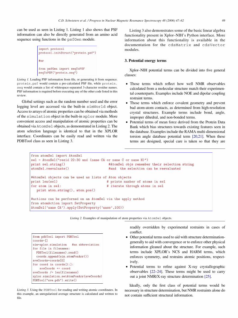
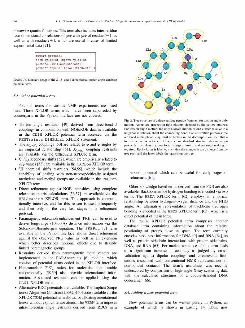
regions of proteins and the base regions of nucleic acids are

generally assumed to be rigidly planar; and, in structure

determination of protein–protein complexes, the constituent

protein structures may be known such that it is desirable to

keep the non-interfacial regions fixed. It is generally not

desirable that these known coordinates be altered. It is also true

that the configuration space of internal coordinates to be

searched in a structure determination calculation can be much

smaller. For instance, the size of torsion angle space is

approximately one third that of Cartesian coordinates for

proteins. Furthermore, larger molecular dynamics timesteps are

possible if high frequency bond-stretching motion is omitted.

For these reasons, it is desirable to perform molecular dynamics

and minimization in internal coordinates.

Molecular dynamics calculations require accelerations in

whichever coordinate system is being used. But efficiently

solving Newton’s equation FZMa for internal coordinate

accelerations a is a nontrivial problem, as the M mass matrix is

full and time-varying. The robotics community has come up

with a clever, efficient solution [67–69] of Newton’s equation

in internal coordinates, with the condition that the structures be

decomposable into tree-like topologies. Fortunately, most

biomolecular systems satisfy this criterion to a good

approximation. In structures with topological loops (with e.g.

sugar rings or disulfide bonds), the loop-causing bond is

replaced with a bonding potential term, or with a bond

constraint. An example of tree decomposition of a three-residue

peptide is shown in Fig. 2.

C.D. Schwieters et al. / Progress in Nuclear Magnetic Resonance Spectroscopy 48 (2006) 47–6256

Xplor–NIH contains an efficient implementation of this

internal coordinate algorithm available in the Python

interface in the ivm module [11]. This implementation

allows arbitrary internal coordinates such as bond stretching,

bending, and torsion angles. Listing 15 displays an example

of topology setup for torsion angle dynamics with a fixed

region.

One can also use the IVM to perform dynamics in the full

Cartesian space and arbitrary mixtures of rigid-body, Cartesian,

Listing 15. Topology setup for torsion angle dynamics with a fixed region composed of residues numbered 100–120, inclusive.

and internal coordinates. A variable timestep MD algorithm is

available which tunes the timestep such that the error in total

energy conservation is kept approximately constant. Finally, the

IVM contains a facility to constrain bonds which cause loops in a

tree. Listing 16 depicts setting up an IVM object for running

molecular dynamics.

Listing 16. Set up and run dynamics coupled to an external temperature bath, using the variable timestep algorithm.

The capabilities of the IVM are used to restrict the allowed

degrees of freedom of the VarTensor object used by RDC

and CSA restraint terms and introduced in Listing 5. The tensor

axis should only rotate, while The P1 and P2 atoms only need

to undergo the specified bending motions, and only if Da or h

are allowed to vary. Listing 17 demonstrates the invocation to

properly set up VarTensor topology.

Listing 17. Topology setup for tensor atoms. The VarTensor’s freedom

member is consulted as to the details of the topology configuration for the axis

parameter atom degrees of freedom.

The IVM is commonly used in simulated annealing

calculations, which consist of performing molecular dynamics

starting at a high temperature, and then slowly decreasing the

temperature in order to find the global minimum region. In

Xplor–NIH annealing protocols, potential parameters are

generally ramped while the temperature is decreased, such

that the potential energy is initially softer, with lower barriers

[70]. As simulated annealing progresses and the temperature is

decreased, force constants are increased such that the potential

takes its desired final form at the end of the annealing

protocol. The helper class AnnealIVM demonstrated in

Listing 18 simplifies and helps to codify the Xplor–NIH

annealing protocols.

Listing 18. Use of the AnnealIVM Simulated Annealing helper class. When the run method is called, simulated annealing is performed from initTemp to

finalTemp, at intervals of tempStep degrees. The length of the dynamics run at each temperature is specified in the setup of the ivm argument illustrated in

Listing 16. The rampedParams list specifies which potential energy parameters to ramp during simulated annealing.

C.D. Schwieters et al. / Progress in Nuclear Magnetic Resonance Spectroscopy 48 (2006) 47–62 57

5. Parallel computation of structures

Multiple NMR structures which differ only in the random

number seed used for initial coordinate and velocity

generation are commonly used for two basic reasons: (1)

to more completely sample the potential surface so that there

is a better chance of finding the region of the global

minimum, and (2) to obtain some information on the range

of structures which are consistent with the NMR data. This

range of structures may or may not be indicative of actual

structural heterogeneity in solution.

Parallel structure computation is handled transparently in

Xplor–NIH using the StructureLoop class, and an example

of its use can be found in Listing 19. Actual parallel execution

is achieved by specifying the -parallel and -machineflags on the xplor (or pyXplor) command-line. [Alter-

natively, on a Scyld cluster, the -scyld flag may be used.]

Listing 19. Schematic use of the StructureLoop class for structure calculation. I

of the -parallel command-line flag.

The current implementation divides Nstructs, the number of

structures, by NCPU, the number of CPUs, and allots each CPU

Nstructs=NCPU structures in a consecutive fashion. The require-

ments for proper operation of this facility include a shared

filesystem which looks identical on each node, fully populated

/bin and /usr/bin directories, and the ability to login to

remote nodes without a password, for instance with ssh.

6. Ensemble refinement

In solution, biomolecules are in constant motion so that NMR

observables generally do not reflect the measurement of a single

conformer, but rather a collection of structures which inter-

convert. Relaxation studies can probe picosecond to nanosecond

timescale dynamics using laboratory frame experiments and

microsecond to millisecond times using rotating frame exper-

iments [71]. Molecular motion can also result in observable

f this class is used, parallel structure calculation is transparently enabled by use

C.D. Schwieters et al. / Progress in Nuclear Magnetic Resonance Spectroscopy 48 (2006) 47–6258

effects on dipolar coupling measurements [13,14], NOE

intensities [72], and other NMR observables.

Xplor–NIH contains well-developed facilities to support

refinement against an ensemble of structures. The invocation

used to create an ensemble of non-interacting structures is shown

in Listing 20. This facility lends itself to local symmetric

multiprocessing (SMP) parallelism, which can be enabled by

specifying a number of parallel threads greater than one using the

-num_threads command-line option. Note that this ensemble

facility does not require the creation of special PSF files, or of

turning off intra-ensemble non-bonded interactions.

Listing 20. Code to create a three-membered ensemble. Creation of the

EnsembleSimulation makes copies of the current atom positions, velocities,

etc. The constituent structures do not interact except by special ensemble-aware

potential terms.

Ensemble-averaged quantities are denoted inside angle

brackets and are calculated as

hxiZXi

Gixi; (7)

where xi is the value of quantity x in ensemble member i, and Gi is

the weight on the ith member. Gi is usually taken to be 1/Ne where

Ne is the ensemble size, but nonuniform weighting is also

supported. Kinetic energy is averaged over the ensemble. Note

that this averaging results in an effective scaling of time by 1/Ne,

an effect which must be taken into account in annealing protocols.

Python potential energy terms include AvePot, which can be

used to average a potential term over the ensemble. That is, the

ensemble-averaged energy of term Ea is just hEai. An example of

the use of AvePot is shown in Listing 21. It is important to note

that this term is inappropriate for NMR observables: the

observable, not the energy, must be properly averaged over the

ensemble. For this reason, the NOEPot, RDCPot, JCoupPotand CSAPot terms recognize the EnsembleSimulation and

calculate the correct ensemble observable. For example, the

correct ensemble NOE sum distance is

rðensÞNOE Z ½h

Xij

jqiKqjjK6i�K1=6; (8)

so that averaging occurs over both the ensemble and over

ambiguous nuclei.

Listing 21. Creation of a simple ensemble-averaged energy term.

There are also some observables which are intrinsically

ensemble quantities, and Xplor–NIH contains support for refining

against two of these: relaxation-derived order parameters, and

crystallographic B-factors.

6.1. Order parameters

Data for generalized order parameters [73] are usually derived

from analysis of relaxation experiments [71]. The S2 order

parameter takes values between 0 and 1, with smaller values of S2

indicating larger heterogeneity, and hence more motion. The

order parameter corresponding to motion of a fixed-length bond is

calculated from an ensemble of structures as [73]

S2 Z1

2

Xij

GiGjð3ðui,ujÞ2K1Þ; (9)

where ui is a unit vector along the appropriate bond vector in

ensemble member i. Order parameters can be reproduced to a

good approximation by refining an ensemble of structures against

high-quality dipolar coupling data [14], but better agreement is

possible by direct refinement against S2 [74]. An example of

OrderPot setup can be seen in Listing 22.

Listing 22. Creation of an order parameter potential term with name s2_nh using

the restraint table named nh_s2.tbl.

6.2. Crystallographic B-factors

The Crystallographic B-factor (or temperature factor) can

directly reflect atomic root mean square displacement. It is

calculated for a single atom as

BZ 8p2hjqiKhq0ij2i; (10)

where q0i is the position of the atom in question in ensemble i,

relative to a molecule-fixed point. hq0i is the ensemble-averaged

value of this quantity. With this definition, intra-ensemble

translation does not contribute to B. An example of creating a

potential term for refining against B-factors is given in Listing 23.

Note that one must exercise care when refining against B-factors,

as they can be skewed by crystallographic packing and non-

motional heterogeneity [74].

Listing 23. Example of creating a B-factor potential term. The structure’s default

fixed point for determining q0 is the average position of all atoms. This can be

modified by specifying the centerSel argument in create_BFactorPot.

6.3. Shape term

This term is introduced to prevent rotation and deformation of

one ensemble member relative to another [13]. Molecular shape

is approximately represented by a massless inertia tensor

analogous to the dipolar coupling alignment tensor. This tensor

can be written as

C.D. Schwieters et al. / Progress in Nuclear Magnetic Resonance Spectroscopy 48 (2006) 47–62 59

Tshape ZXi

y2i Cz2

i Kxiyi Kxizi

Kxiyi x2i Cz2

i Kyizi

Kxizi Kyizi x2i Cy2

i

0BB@

1CCA; (11)

where xi, yi, and zi are the components of the Cartesian coordinate

of atom i, relative to the center position. The sum is over all atoms

used to define molecular shape.

The associated energy is then defined in terms of the principal

values of the shape tensors of ensemble member structures:

Eshape Zworient

Xi;j

GiGjVpQuadðFi;j;DF;DFÞ

Cwsize

Xi;j

GiGj

Xa

VpQuadðliaKlja;Dl;DlÞ; (12)

where Fi;j is the magnitude of the rotation of the principal axes of

ensemble member i relative to those of ensemble member j, and

lia is the value of eigenvalue (principal value) a for ensemble

member i. worient and wsize are scale factors, DF and Dl denote

the allowed deviations, the a sum is over the three principal axes,

and the i, j sums are over all pairs of ensemble members. An

example of setting up this potential term can be seen in Listing 24.

Listing 24. Example of creating a ShapePot term which restrains the orientation

and size of the shape tensor composed of all C atoms.

In practice it has been found that this term is too crude to aid in

preventing deformation and rotation of one ensemble member

relative to another, as the whole protein is described as an

ellipsoid. A more successful approach is to use separate instances

of this term for each secondary structure element. The RAP term

discussed below can be used to enforce much more rigid

similarity between ensemble members.

6.4. Constraining relative atom position with RAPPot

Finally, Xplor–NIH contains an ensemble potential which

prevents atom positions from drifting too far apart—this is useful

to help refinement calculations converge [13].

ERAP ZwRAP

Xi

hVpQuadðjq0iKhq0

iij;DlRAP;DlRAPi; (13)

where wRAP is a constant scale factor, q0i is defined in Section 2,

DlRAP is the allowed distance deviation, VpQuad is defined in Eq.

(1), and the sum is over all atoms to be restrained. An example of

setting up this potential term can be seen in Listing 25.

Listing 25. Example of creating an RAPPot which restrains the positions of Ca

atoms to be within 0.3 A of the average position for all members of an ensemble.

7. Other Xplor–NIH facilities

7.1. Probabilistic NOE assignment algorithm for automated

structure determination (PASD)

Xplor–NIH includes the PASD facility for automatic NOE

assignment from completely automatically peak-picked multi-

dimensional NMR spectra, with simultaneous structure determi-

nation [12]. The key features of this facility are:

† Probabilistic selection of good NOE assignments with no

peaks ever permanently discarded.

† For a given NOE peak, multiple possible assignments are

simultaneously enabled.

† A linear NOE potential is used in early stages of the

calculation so that all assignments contribute equal magnitude

forces.

† Successive passes of assignment calculation are not based on

previously determined structures, thus greatly reducing the

chances of converging on incorrect structure/assignment

combinations.

More details can be found in Ref. [12].

The PASD algorithm has been found to be highly robust in the

face of bad NOE data (including missing or bad chemical shift

assignments), with the ability to tolerate about 80% bad long-

range data (i.e data between residues whose sequence position is

more than 5 residues apart). Failure of the method is clearly

indicated by lack of convergence of assignment likelihoods, and

by a large value for the precision of the calculated ensemble of

structures. The following input formats are currently supported:

nmrdraw, nmrstar, pipp, and xeasy. It is a simple task to write

filters to support additional formats.

The user interface to PASD is a set of Tcl scripts, examples of

which can be found in the eginput/marvin/* subdirectories

of the Xplor–NIH distribution. These scripts are written at a very

high level and are easy to modify.

7.2. VMD–XPLOR interface

Xplor–NIH contains interfaces to the VMD-XPLOR [15]

molecular graphics package, a version of the VMD (visual

molecular dynamics) program [75] which has been customized

for NMR structure determination. These interfaces can be used to

load structures, labels and trajectories from Xplor–NIH, and can

be used to run structure calculations on one computer while

displaying the results on another. Graphical objects in VMD are

C.D. Schwieters et al. / Progress in Nuclear Magnetic Resonance Spectroscopy 48 (2006) 47–6260

accessed via instances of object entities within the Python

interface. An example of fitting two structures and displaying

them in the VMD graphical window is shown in Listing 26. Note

that there is also an XPLOR interface to VMD-XPLOR accessed

via the PS statement.

Listing 26. A complete script demonstrating loading two structures and displaying them using a running instance of the the VMD–XPLOR graphical package. The -

host and -port xplor command-line options must be appropriately set to make a successful connection.

7.3. Analysis and validation

Information on how well a given structure satisfies experimen-

tal restraints is given in the standard structure files produced by the

StructureLoop class introduced in Listing 19. The resulting

structure files contain a summary of the number of restraints which

are violated by more than a given standard (but adjustable)

threshold value, and the root-mean-square deviation of the

difference between calculated and experimental observables. A

detailed listing of the specific violations for each term is given in a

separate file with a .viols suffix. If the averageFilenameand averagePotList arguments are given to the Struc-tureLoop constructor, a regularized average structure is

generated which also contains precision information about the

calculated ensemble. Final validation of a structure may include

cross-validation [76,77] of NMR observables, as well as the use of

an external tool such as PROCHECK [78] or WhatIf [79].

7.4. Test suite

Xplor–NIH is distributed with a full suite of regression tests

both in the source and binary-only packages. These tests are

essential to obtain confidence that the package operates properly.

For end-users, possible problems can be caused by moving to a

system with slightly different hardware or operating system

configuration from those used for compilation. For developers, a

seemingly unrelated change might break some other functionality

within Xplor–NIH. These tests provide some assurance that the

package does indeed behave as it is expected to, and allows quick

identification as to where an error is located. In the source package,

components are tested hierarchically: the CCC template library

contains a test suite, as does the IVM and each potential term. In

both the source and binary distributions the XPLOR, Python and

Tclinterfaces contain a large collection of test scripts along with the

expected output. The bin/testDist command invokes an

automated procedure which runs each script and reports

discrepancies. These tests are essential to validate a new

installation of Xplor–NIH.

Extensive sets of full scripts with all supporting data are

present in the eginput and tutorial subdirectories of a

Xplor–NIH distribution. Basic validation of the suite of example

scripts in the eginput subdirectory is performed using the

runAll script in that directory.

8. Conclusion

This review has provided an overview of using the Xplor–NIH

suite for NMR structure determination, focusing primarily on the

C.D. Schwieters et al. / Progress in Nuclear Magnetic Resonance Spectroscopy 48 (2006) 47–62 61

Python interface. The example code here is by necessity

fragmentary and incomplete. Many facilities have not been

touched upon at all. Much more complete documentation is

available from the Xplor–NIH website. Specific questions should

be addressed to the Xplor–NIH mailing list at Xplor–NIH@nmr.

cit.nih.gov.

Acknowledgements

Again it should be emphasized that many of the components

of this package are the product of a large number of workers over

two decades. In particular, the Xplor–NIH software package owes

a great debt to Axel Brunger as the original creator of XPLOR. In

addition, major contributions have been made by Michael Nilges

and the original developers of CHARMM [80] and CNS [16]. We

also thank the groups of Nico Tjandra, Ad Bax and Andy Byrd for

valuable contributions.

This work was supported by the following Intramural

Research programs of the NIH: CIT, NIDDK, NCI, and NHLBI.

References

[1] C.D. Schwieters, J.J. Kuszewski, N. Tjandra, G.M. Clore, J. Magn. Reson.

160 (2003) 66–74.

[2] A.T. Brunger, XPLOR Manual Version 3.1 . Yale University Press, New

Haven; 1355. Available online at http://xplor.csb.yale.edu/xplor-info/.

[3] J. Kuszewski, A.M. Gronenborn, G.M. Clore, J. Am. Chem. Soc. 121 (1999)

2337–2338.

[4] N. Tjandra, J. Marquardt, G.M. Clore, J. Magn. Reson. 142 (2000) 393–396.

[5] G. Cornilescu, A. Bax, J. Am. Chem. Soc. 122 (2000) 10143–10154.

[6] L. Banci, I. Bertini, G. Cavallaro, A. Giachetti, C. Luchinat, G. Parigi,

J. Biomol. NMR 28 (2004) 249–261.

[7] J. Iwahara, C.D. Schwieters, G.M. Clore, J. Am. Chem. Soc. 126 (2004)

5879–5896.

[8] J. Kuszewski, G.M. Clore, J. Magn. Reson. 146 (2000) 249–254.

[9] J. Kuszewski, C.D. Schwieters, G.M. Clore, J. Am. Chem. Soc. 123 (2001)

3903–3918.

[10] G.M. Clore, J. Kuszewski, J. Am. Chem. Soc. 124 (2002) 2866–2867.

[11] C.D. Schwieters, G.M. Clore, J. Magn. Reson. 152 (2001) 288–302.

[12] J. Kuszewski, C.D. Schwieters, D.S. Garrett, R.A. Byrd, N. Tjandra,

G.M. Clore, J. Am. Chem. Soc. 126 (2004) 6258–6273.

[13] G.M. Clore, C.D. Schwieters, J. Am. Chem. Soc. 126 (2004) 2923–2938.

[14] G.M. Clore, C.D. Schwieters, Biochemistry 43 (2004) 10678–10691.

[15] C.D. Schwieters, G.M. Clore, J. Magn. Reson. 149 (2001) 239–244.

[16] A.T. Brunger, P.D. Adams, G.M. Clore, W.L. DeLano, P. Gros,

R.W. Grosse-Kunstleve, J.-S. Jiang, J. Kuszewski, M. Nilges, N.S. Pannu,

R.J. Read, L.M. Rice, T. Simonson, G. Warren, Acta Crystallogr. Ser. D 54

(1998) 905–921.

[17] Available online at: http://www.swig.org/

[18] M. Lutz, D. Ascher, Learning Pythonsecond ed. O’Reilly, Sebastopol, CA,

2004 Available online at: http://python.org.

[19] Available online at: http://nmr.cit.nih.gov/xplor-nih/doc/current/python/ref/

index.html

[20] J. Kuszewski, A.M. Gronenborn, G.M. Clore, Protein Sci. 5 (1996) 1067–1080.

[21] J. Kuszewski, A.M. Gronenborn, G.M. Clore, J. Magn. Reson. 125 (1997)

171–177.

[22] A.T. Brunger, J. Kuriyan, M. Karplus, Science 235 (1987) 458–460.

[23] A.T. Brunger, in: N.W. Isaacs, M.R. Taylor (Eds.), Crystallographic

Computing 4: Techniques and New Technologies, Clarendon Press, Oxford,

1988, pp. 126–140.

[24] A.T. Brunger, Nature 355 (1992) 472–475.

[25] B. Shaanan, A.M. Gronenborn, G.H. Cohen, G.L. Gilliland,

B. Veerapandian, D.R. Davies, G.M. Clore, Science 257 (1992) 961–964.

[26] M. Nilges, A.M. Gronenborn, A.T. Brunger, G.M. Clore, Protein Eng. 2

(1988) 27–38.

[27] M. Nilges, Proteins 17 (1993) 297–309.

[28] K. Wuthrich, M. Billeter, W. Braun, J. Mol. Biol. 169 (1983) 949–961.

[29] A. Bax, G. Kontaxis, N. Tjandra, Methods Enzymol. 339 (2001)

127–174.

[30] N. Tjandra, J.G. Omichinski, A.M. Gronenborn, G.M. Clore, A. Bax, Nat.

Struct. Biol. 4 (1997) 732–738.

[31] G.M. Clore, A.M. Gronenborn, N. Tjandra, J. Magn. Reson. 131 (1998) 159–

162.

[32] Z. Wu, N. Tjandra, A. Bax, J. Am. Chem. Soc. 123 (2001) 3617–3618.

[33] R.S. Lipsitz, N. Tjandra, J. Am. Chem. Soc. 123 (2001) 11065–11066.

[34] M. Ottiger, A. Bax, J. Am. Chem. Soc. 119 (1997) 8070–8075.

[35] D.S. Garrett, J. Kuszewski, T.J. Hancock, P.J. Lodi, G.W. Vuister,

A.M. Gronenborn, G.M. Clore, J. Magn. Reson. Ser. B 104 (1994)

99–103.

[36] R.A. Engh, R. Huber, Acta Crystallogr. A 47 (1991) 392–400.

[37] W. Braun, N. Go, J. Mol. Biol. 186 (1985) 611–626.

[38] G. Nemethy, M.S. Pottle, H.A. Scheraga, J. Phys. Chem. 87 (1983) 1883–

1887.

[39] W.L. Jorgensen, J. Tirado-Rives, J. Am. Chem. Soc. 110 (1988) 1666–1671.

[40] S.J. Weiner, P.A. Kollman, D.A. Case, U.C. Singh, C. Ghio, G. Alagona,

S. Profeta, P. Weiner, J. Am. Chem. Soc. 106 (1984) 765–784.

[41] A.W. Schuettelkopf, D.M.F. van Aalten, Acta Crystallogr. D60 (2004) 1355–63

Available online at: http://davapc1.bioch.dundee.ac.uk/programs/prodrg/.

[42] G.J. Kleywegt, J.Y. Zou, M. Kjeldgaard, T.A. Jones,

M.G. RossmannE. Arnold International Tables for Crystallography, Vol. F.

Crystallography of Biological Macromolecules . Kluwer Academic Publish-

ers, Dordrecht; pp. 353–356 (see also pp. 366–367) Available online at:

http://xray.bmc.uu.se/gerard/manuals/xplo2d_man.html.

[43] M. Nilges, G.M. Clore, A.M. Gronenborn, FEBS Lett. 229 (1988) 317–324.

[44] J.P. Linge, M. Nilges, J. Biomol. NMR 13 (1999) 51–59.

[45] J.P. Linge, M.A. Williams, C.A.E.M. Spronk, A.M.J.J. Bonvin, M. Nilges,

Proteins 50 (2003) 496–506.

[46] S.B. Nabuurs, A.J. Nederveen, W. Vranken, J.F. Doreleijers,

A.M.J.J. Bonvin, G.W. Vuister, G. Vriend, C.A.E.M. Spronk, Proteins 55

(2004) 483–486.

[47] T. Simonson, Curr. Opin. Struct. Biol. 11 (2001) 243.

[48] J. Skolnick, A. Kolinski, A.R. Ortiz, J. Mol. Biol. 265 (1997) 217–241.

[49] G.M. Clore, M. Nilges, D.K. Sukumaran, A.T. Brunger, M. Karplus,

A.M. Gronenborn, EMBO J. 5 (1986) 2729–2735.

[50] J. Kuszewski, G.M. Clore, unpublished.

[51] G.W. Vuister, F. Delaglio, A. Bax, J. Biomol. NMR 3 (1993) 67–80.

[52] J. Kuszewski, J. Qin, A.M. Gronenborn, G.M. Clore, J. Magn. Reson. Ser. B

106 (1995) 92–96.

[53] S. Spera, A. Bax, J. Am. Chem. Soc. 113 (1991) 5490–5492.

[54] J. Kuszewski, A.M. Gronenborn, G.M. Clore, J. Magn. Reson. Ser. B 107

(1995) 293–297.

[55] J. Kuszewski, A.M. Gronenborn, G.M. Clore, J. Magn. Reson. Ser. B 112

(1996) 79–81.

[56] P. Yip, D.A. Case, J. Magn. Reson. 83 (1989) 643–648.

[57] M. Nilges, J. Habazettl, A.T. Brunger, T.A. Holak, J. Mol. Biol. 219 (1991)

499–510.

[58] N. Tjandra, D.S. Garrett, A.M. Gronenborn, A. Bax, G.M. Clore, Nat. Struct.

Biol. 4 (1997) 443–449.

[59] G.M. Clore, A.M. Gronenborn, A. Szabo, N. Tjandra, J. Am. Chem. Soc. 120

(1998) 4889–4890.

[60] H.J. Sass, G. Musco, S.J. Stahl, P.T. Wingfield, S. Grzesiek, J. Biomol. NMR

21 (2001) 275–280.

[61] J. Meiler, N. Blomberg, M. Nilges, C. Griesinger, J. Biomol. NMR 16 (2000)

245–252.

[62] R.S. Lipsitz, Y. Sharma, B.R. Brooks, N. Tjandra, J. Am. Chem. Soc. 124

(2002) 10621–10626.

[63] A. Grishaev, A. Bax, J. Am. Chem. Soc. 126 (2004) 7281–7292.

[64] G.M. Clore, J. Kuszewski, J. Am. Chem. Soc. 125 (2003) 1518–1525.

[65] J. Kuszewski, G.M. Clore, unpublished.

[66] X. Zuo, D.M. Tiede, J. Am. Chem. Soc. 127 (2005) 16–17.

[67] Dae-Sung Bae, E.J. Haug, Mech. Struct. Mach. 15 (1987) 359.

C.D. Schwieters et al. / Progress in Nuclear Magnetic Resonance Spectroscopy 48 (2006) 47–6262

[68] G. Rodriguez, A. Jain, K. Kreutz-Delgado, J. Austron. Sci. 40 (1992) 27.

[69] A. Jain, N. Vaidehi, G. Rodriguez, J. Comput. Phys. 106 (1993) 258.

[70] G.M. Clore, A.M. Gronenborn, CRC Crit. Rev. Biochem. Mol. Biol. 24

(1989) 479–564.

[71] A.G. Palmer III, Annu. Rev. Biophys. Biomol. Struct. 30 (2001) 129–155.

[72] D.A. Pearlman, P.A. Kollman, J. Mol. Biol. 220 (1991) 457–479.

[73] G. Lipari, A. Szabo, J. Am. Chem. Soc. 104 (1982) 4559–4570.

[74] G.M. Clore, C.D. Schwieters, J. Mol. Biol. in press.

[75] W. Humphrey, A. Dalke, K. Schulten, J. Mol. Graphics. 14 (1996) 33–8

Available online at: http://www.ks.uiuc.edu/Research/vmd/.

[76] A.T. Brunger, G.M. Clore, A.M. Gronenborn, R. Saffrich, M. Nilges, Science

261 (1993) 328–331.

[77] G.M. Clore, D.S. Garrett, J. Am. Chem. Soc. 121 (1999) 9008–9012.

[78] R.A. Laskowski, M.W. MacArthur, D.S. Moss, J.M. Thornton, J. Appl.

Crystallogr. 26 (1993) 283–91 Available online at: http://www.biochem.ucl.

ac.uk/roman/procheck/procheck.html.

[79] R.W.W. Hooft, G. Vriend, C. Sander, E.E. Abola, Nature. 381 (1996) 272

Available online at: http://swift.cmbi.kun.nl/whatif/.

[80] B.R. Brooks, R.E. Bruccoleri, B.D. Olafson, D.J. States, S. Swaminathan,

M. Karplus, J. Comput. Chem. 4 (1983) 187–217.