NDT JAMES INSTRUMENTS INC. NON DESTRUCTIVE TESTING SYSTEMS V-METER INSTRUCTION MANUAL MARK II 3727 N. Kedzie Avenue. Chicago, Illinois 60618 Telex - 206729U.D 1-800-426-6500 (312) 463-6565 Fax: (312) 463-0009

TABLE OF CONTENTS

SECTION 1

PRINCIPALS OF TESTING BY ULTRASONIC PULSE VELOCITY MEASUREMENT 1.1 Introduction 1 1.2 Velocity of Longitudinal pulses in Elastic Solids 1 1.3 Effect of Size and Shape of Specimen Tested 2 1.4 Frequency of Pulse Vibrations 2 1.5 Method of Testing 2 1.6 Application of Pulse Velocity Testing 4

SECTION II

SPECIFICATION OF V-METER MK II

2.1 The V-Meter MK II 6 2.2 The V-Meter Field Kit C-7901 6 2.3 Description 6 2.4 Construction of the V-Meter MK II 8 2.5 Transducers and Leads 8 2.6 Summary of Specifications 9

SECTION III

OPERATING INSTRUCTIONS 3.1 Introduction 11 3.2 General Description 11 3.3 Initialization Items Explained 15 3.4 Menu Items - Main Menu 17 3.5 Menu Items - Run Menu 20 3.6 Familiarization 20 3.7 Summary 24 3.8 Addenda 24 3.9 A.C Operation 24 3.10 Battery Operation 25 3.11 Full Charging the Internal Battery 25

SECTION IV

TAKING PULSE VELOCITY MEASUREMENTS

4.1 Transducers 26 4.2 Offset (Zero Set) 26 4.3 Couplant 26 4.4 Placing the Transducers 26 4.5 Pulse Velocity 27

SECTION V

SYSTEM DESCRIPTION

5.1 Pulse Generator 29 5.2 CPU 29 5.3 Receiver Amplifier 29 5.4 Master Clock ADC and Display 29

SECTION VI

TESTING CONCRETE

6.1 Applications 30 6.2 Accuracy 30 6.3 Coupling the Transducers with Concrete Surface 31 6.4 Choice of Transducer Arrangement 31 6.5 Influence of Test Conditions 35 6.6 Homogeneity of the Concrete 39 6.7 Detection of Defects 40 6.8 Detection of Large Voids or Cavities 40 6.9 Estimating the Depth of Surface Cracks 40 6.10 Monitoring Changes in Concrete with Time 44 6.11 Estimation of Strength After Fire Damage 44 6.12 Estimation of Strength 48 6.13 Estimation of Elastic Modulus 51 6.14 Determination of the Dynamic Modulus of Elasticity

And Dynamic Poisson's Ratio 53

SECTION VII

ADDITIONAL ACCESSORIES FOR USE WITH THE V-METER MK II

7.1 Longitudinal P-Wave Transducer 56 7.2 Shear Wave Transducers 56 7.3 Different Shape Transducers 56 7.4 Pre-Amplifier - Type C-4896 56 7.5 Pre-Amplifier - Type C-4940 58 7.6 Hand Held Terminal 58

References 59

SECTION I

PRINCIPALS OF TESTING BY ULTRASONIC PULSE VELOCITY MEASUREMENT

1.1 INTRODUCTION The velocity of ultrasonic pulses traveling in a solid material depends on the density and elastic properties of that material. The quality of some materials is sometimes related to their elastic stiffness so that measurement of ultrasonic pulse velocity in such materials can often be used to indicate their quality as well as to determine their elastic properties. Materials which can be assessed in this way include, in particular, concrete and timber but exclude metals. When ultrasonic testing is applied to metals its object is to detect internal flaws which send echoes back in the direction of the incident beam and these are picked up by a receiving transducer. The measurement of time taken for the pulse to travel from a surface to a flaw and back again enables the position of the flaw to be located. Such a technique cannot be applied to heterogeneous materials like concrete or timber since echoes are generated at the numerous boundaries of the different phases within these materials resulting in a general scattering of pulse energy in al directions. 1.2 VELOCITY OF LONGITUDINAL PULSES IN ELASTIC SOLIDS

It can be shown that the velocity of a pulse of longitudinal ultrasonic vibrations traveling in an elastic solid is given by:

where E is the dynamic elastic modulus where p is the density where µ is the Poisson's ratio.

1

2

1.3 EFFECT OF SIZE AND SHAPE OF SPECIMEN TESTED The above equation may be considered to apply to the transmission of longitudinal pulses through a solid of any shape or size provided the least lateral dimension (i.e the dimension measured perpendicular to the path traveled by the pulse) is not less than the wavelength of the pulse vibrations. The pulse velocity is not affected by the frequency of the pulse so that the wavelength of the pulse vibrations is inversely proportional to its frequency.

Thus the pulse velocity will generally depend only on the properties of the materials and the measurement of this velocity enables an assessment to be made of the condition of the materials. 1.4 FREQUENCY OF PULSE VIBRATIONS The pulse frequency used for testing concrete or timber is much lower than that used in metal testing. The higher the frequency, the narrower the beam of pulse propagation but the greater the attenuation (or damping out) of the pulse vibrations. Metal testing requires high frequency pulses to provide a narrow beam of energy but such frequencies are unsuitable for use with heterogeneous and coarse grain materials because of the considerable amount of attenuation which pulses undergo when they pass through these materials. The frequencies suitable for these materials range from about 20 kHz to 250 kHz, which 50 kHz being appropriate for the field testing of concrete. These frequencies correspond to wavelength ranging from about 8 inches ( for the lower frequency) to about .6 inches at the higher frequency. 1.5 METHOD OF TESTING For assessing the quality of materials from ultrasonic pulse velocity measurement, it is necessary for this measurement to be of a high order of accuracy. This is done using an apparatus which generates suitable pulses and accurately measures the time of their transmission (i.e transit time) through the material tested. The distance which the pulse travel in the material (i.e the path length) must also be measured to enable the velocity to be determined from:

3

4

Path length Pulse velocity = ____________

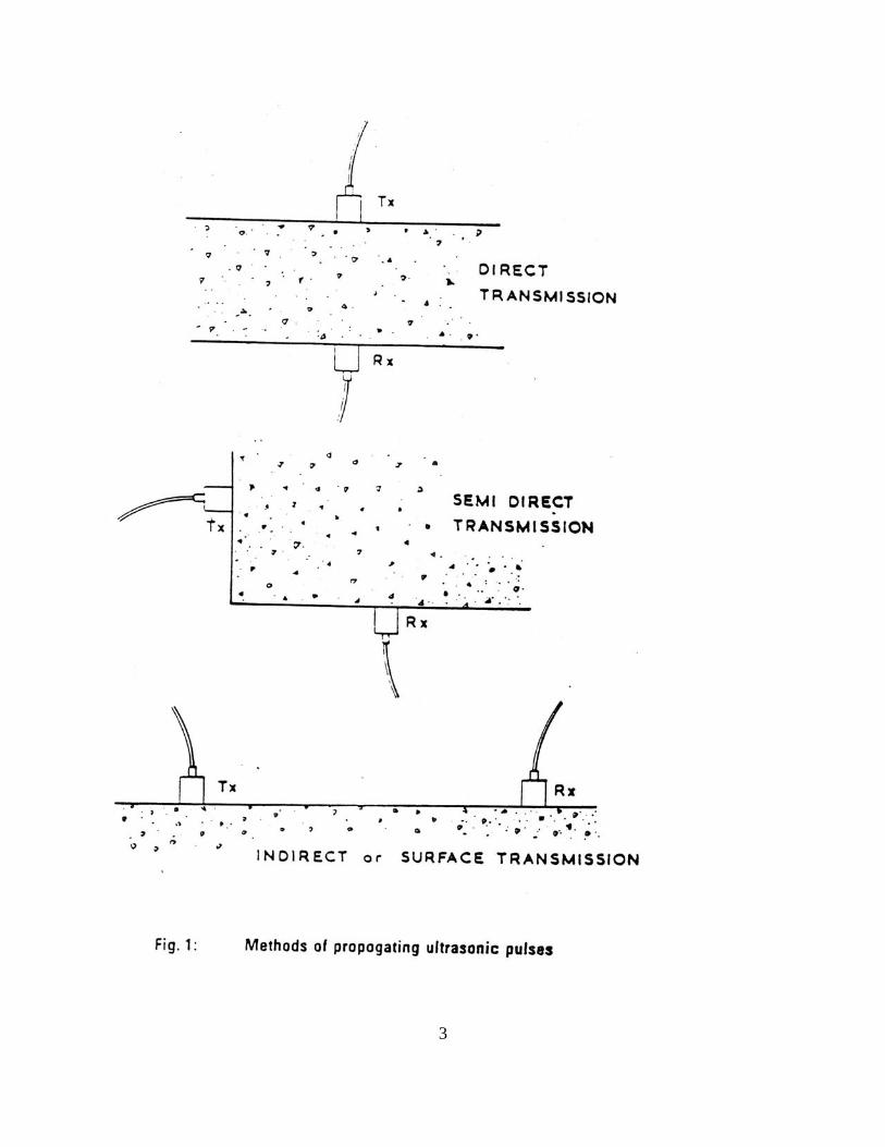
Transit Time Path lengths and transit time should each be measured to an accuracy of about + 1%. The instrument indicates the time taken for the earliest part of the pulse to reach the receiving transducer measures from the time it leaves the transmitting transducer when these transducers are placed at suitable points on the surface of the material. Figure 1 shows how the transducer may be arranged on the surface of the specimen tested, the transmission being either direct, semi direct or indirect. The direct transmission arrangement is the most satisfactory since the longitudinal pulses leaving the transmitter are propagated mainly in the direction normal to the transducer face. The indirect arrangement is possible because the ultrasonic beam of energy is scattered by discontinuities within the material tested but the strength of the pulse detected in this case is only about 1 or 2% of the detected for the same path length when the direct transmission arrangement is used. Pulses are not transmitted through large air voids in a material and, if such a void lies directly in a pulse path, the instrument will indicate the tome taken by the pulse which circumvents the void by the quickest route. It is thus possible to detect large voids when a grid of pulse velocity measurements is made over a region in which these voids are located. 1.6 APPLICATION OF PULSE VELOCITY TESTING This method of testing was originally developed for use on concrete and the published accounts of its application are concerned predominately with this material A considerable volume of literature has been published over the past 40 years describing the results of research on the use of ultrasonic testing for concrete and for fuller details of this application the reader is referred to the selected list given at the end of this Section. The method was first developed in Canada by Leslie and Cheesman between 1945 and 1949 and also independently in Britain at about the same time by Jones and Gatfield. The apparatus developed at that time made use of a cathode-ray oscilloscope for the measurement of transit times and modified forms of this equipment have been widely used in many countries. The equipment was particularly useful in the laboratory but was less easy to use under field conditions. The apparatus described in this Manual has been designed particularly for field testing being light, portable and simple to use. It can be operated independently of the main power supply when used in the field and directly from the A.C. supply for laboratory use.

5

There has been a steadily growing interest in no-destructive testing of concrete in several countries and, a Symposium held in Canada in 1984 and recently in Britain enabled reviews and accounts of current research on the subject to be discussed and recorded. ASTM has the specification ASTMC-597 for the use of this method since 1967 and the British Standards Institution has issued Recommendations for measurement of velocity of ultrasonic pulses in concrete. B.S. 1881: Part 203. 1986. Ultrasonic testing is now widely used throughout the world and it is clear that the advantages of this method over traditional methods of testing are likely to increase further its application. In particular its ability to examine the state of concrete in depth is unrivaled. The pulse velocity method has been shown to provide a reliable means of estimating the strength of timber and has been used to test various kinds of timber products. It is in use for the detection of rot in utility poles and provides a very economic method of inspecting these poles while in service. The same equipment can be used to test rock strata and to provide useful data for geological survey work. The method has also been used for testing graphite, ceramics and any coarse grain materials and it is likely that it will prove useful for testing other non-metallic materials.

6

SECTION II SPECIFICATION OF V-METER MK II 2.1 THE V-METER MK II The V-Meter MK II has been designed with site testing particularly in ind so as to be fully portable, simple to operate and with a high order of accuracy and stability. It generates low frequency ultrasonic pulses and measures the time taken for them to pass from one transducer to the other through the material interposed between them. 2.2 THE V-METER MK II FIELD KIT, C-7901 The complete system comprises the following items:

a) The V-Meter MK II b) Two transducers (54 kHz) c) Two transducer leads d) Carrying case e) V-Meter MK II manual f) Can of couplant g) AC / charger unit.

The optional extras available include:

Transducers with different frequencies. C-4860 hand held terminal Pre-amplifier with x 7 and x 4 gain. Extra long transducer leads up to 100 feet in length. S wave transducers.

2.3 DESCRIPTION The V-Meter Mk II gives a direct reading of the time of transmission of an ultrasonic pulse passing from a transmitting to a receiving transducer, up to 6400 micro seconds, with resolutions of 0.1 micro seconds which represents approximately 100 ft. of concrete. If the transmitted pulse is not received, or when the transducers are removed from the test piece, the LCD will automatically show the maximum number, approximately 6400 micro seconds. No reference calibration bar is needed because the built in micro computer remembers the delay due to the different transducers and cables when first initialized and then subtracts from the following measurement automatically.

7

The pulse generator may be operated at a high voltage of either 1,200 V or 500V as selected by a switch on the top panel. Generally, for concrete testing and for long path lengths the generator is operated at 1,200V but, if fine racks are being investigated it may be advantageous to reduce the high voltage to 500V. Pulse repetition frequencies of 1, 3 and 10 may be selected by a menu driven initialization procedure. The LCD read out is updated once, twice or five times per second for both PRFs depending on the pulse repetition rate. The receiving amplifier has a high input impedance enabling the instrument to be used with piezo-electric and ferro-electric transducers over the frequency range 5kHz to 1MHz. For field use an internal Nickel Cadmium battery will, when fully charged, supply power for about 8 hours continuous use. The battery voltage is monitored by a micro-power sensor which, when the voltage is near to the discharge end point, will cause the low battery LED on the front panel to light up. When the instrument is used on the A.C. mains a built in constant current charger will continuously trickle charge the battery. A fully discharged batter should be charged as soon as possible by connecting the instrument to the A.C. mains, for a 16 hour overnight charge. A cathode ray oscilloscope may be coupled to the CRO and Time Base Trigger BNC sockets mounted on the panels. Both transit time, pulse waveform, and attenuation observations and measurements may be made by using the V-Meter Mk II in conjunction with the CRO. MEMORY OPTION See Section III 4.5 and 8. 2.4 CONSTRUCTION OF THE V-METER MK II The electronic circuit of V-Meter Mk II uses high speed CMOS (74HC) integrated circuits, and a micro computer chip with E-prom. The assembly is designed for ease of access for servicing the component boards. 2.5 TRANSDUCERS AND LEADS The transducers consist of lead zirconate titanate (PZT4) ceramic piezo electric elements mounted in stainless steel cases. The elements are very tightly held on to the inside face of the case to provide highly efficient acoustic transmission. The transducer assembly is very robust and able to withstand reasonably rough conditions as normally encountered under conditions of industrial usage.

8

The shock excitation of the pulse generator causes the transducer to oscillate mechanically at its own natural frequency, this frequency depending on the size and stiffness of the whole transducer assembly. Different sizes of piezo electric element and case enable different pulse frequencies to be obtained. Each transducer is fitted with a cable socket to enable it to be detached from the cable and to allow cables of different length to be used. Short co-axial cables for connecting the transducers to the V-Meter Mk II are supplied with the instrument. Longer cables may be used when access to the areas to be tested is restricted. Although long cables reduce the size of both the transmitted pulse and the receiving signal, these are generally both of adequate magnitude for testing even when the cables are 25 ft. long. Note: The instrument should be re-zeroed when changing to long cables. A delay of about 0.8 microsecs. Is introduced when using 100 ft. cables on both the transmitting and receiving transducers. To minimize attenuation when using long cables, a signal amplifier, with a low output impedance, can be inserted between the receiving transducer and the cable. 2.6 SUMMARY OF SPECIFICATION TRANSIT TIME MEASUREMENT RANGE 0.1 micro sec to 6400 micro sec. 0.1 micro

second timing pulses derived from a 10 MHz crystal oscillator.

Accuracy ±0.1 micro sec.

Lost signal 6400 micro seconds.

INPUT SENSITIVITY: 250 micro volt between 36 kHz 500 kHz.

Signal Instrument may be used with frequencies outside this range but with reduced sensitivity.

Impedance Approximately 2MOHMS.

TRANSMITTER:

Energizing pulse Nominal 1.2kV or 500V, switch selected.

Discharge time Depends on transducer and cable length. With 54 kHz transducers and 50 ft. of cable discharge time about 1.5 milli sec.

9

PRF 1, 3 or 100pps derived from 10MHz crystal,

selected by menu. POWER SUPPLY: Internal rechargeable Nicad battery.

Capacity for about 9 hours continuous use.

Battery low Indicated by the battery low LED.

Battery Charger Supplied with unit, 12V DC with built-in constant current charger. Battery is trickle charged continuously when instrument is connected to the A.C. mains.

Display 240 x 64 dot matrix reflective LCD.

Temp. Range 0°C to 40 °C.

OUTPUTS CRO output:

Received signal Available from BNC socket on front panel. True facsimile of received signal for outputs up to 0.4V. For outputs in excess of this value the receiving transducer may be plugged directly into the CRO with the Time Base synchronized from the instrument.

Time Base Sync. Pulse A 3.5V positive pulse with a rise time of 2

micro sec is also available from a BNC socket on the rear panel.

OPTION Hand held terminal with memory capacity of

100 readings to upload to PC and data manipulation.

10

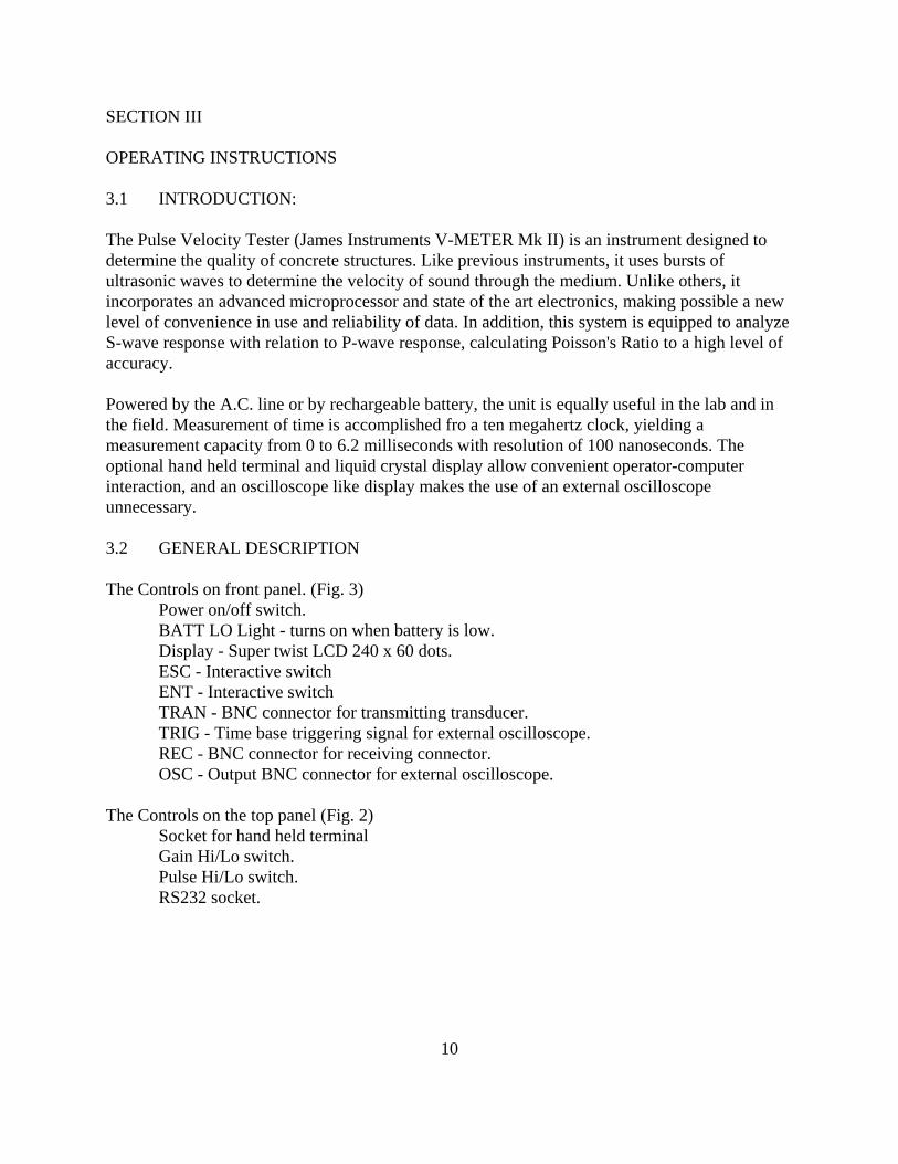
SECTION III OPERATING INSTRUCTIONS 3.1 INTRODUCTION: The Pulse Velocity Tester (James Instruments V-METER Mk II) is an instrument designed to determine the quality of concrete structures. Like previous instruments, it uses bursts of ultrasonic waves to determine the velocity of sound through the medium. Unlike others, it incorporates an advanced microprocessor and state of the art electronics, making possible a new level of convenience in use and reliability of data. In addition, this system is equipped to analyze S-wave response with relation to P-wave response, calculating Poisson's Ratio to a high level of accuracy. Powered by the A.C. line or by rechargeable battery, the unit is equally useful in the lab and in the field. Measurement of time is accomplished fro a ten megahertz clock, yielding a measurement capacity from 0 to 6.2 milliseconds with resolution of 100 nanoseconds. The optional hand held terminal and liquid crystal display allow convenient operator-computer interaction, and an oscilloscope like display makes the use of an external oscilloscope unnecessary. 3.2 GENERAL DESCRIPTION The Controls on front panel. (Fig. 3)

Power on/off switch. BATT LO Light - turns on when battery is low. Display - Super twist LCD 240 x 60 dots. ESC - Interactive switch ENT - Interactive switch TRAN - BNC connector for transmitting transducer. TRIG - Time base triggering signal for external oscilloscope. REC - BNC connector for receiving connector. OSC - Output BNC connector for external oscilloscope.

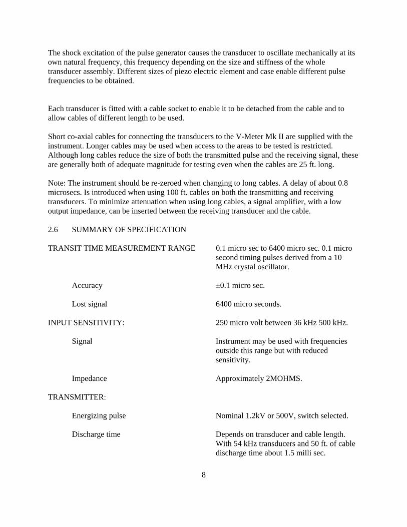
The Controls on the top panel (Fig. 2)

Socket for hand held terminal Gain Hi/Lo switch. Pulse Hi/Lo switch. RS232 socket.

11

12

13

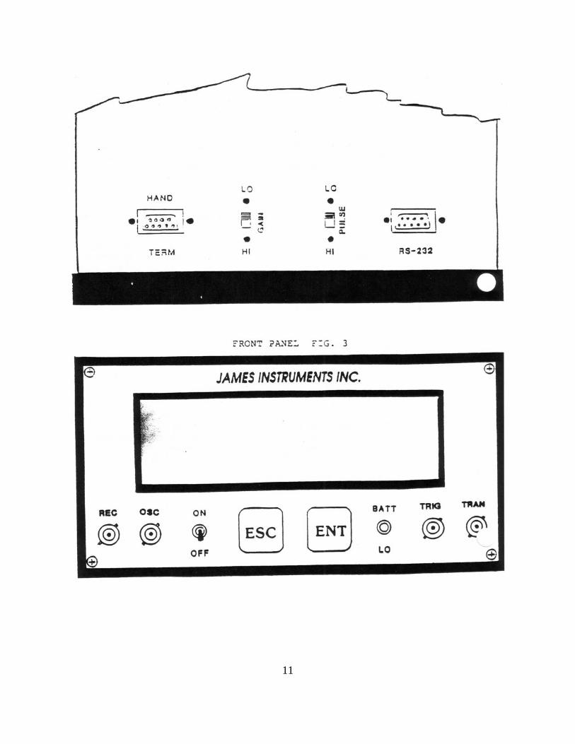
The Controls on the back panel (Fig. 4) Charger - Accept the charger plug Light - EL light of LCD on / off switch Display contrast - to adjust the contrast on display.

The High/Low gain switch compensates for distance, increasing or decreasing the signal strength presented to the electronics. Pulse level, which should be low at short distances, is set by the High/Low pulse switch on the top panel. The contrast control may be adjusted for optimum viewing comfort as the battery condition changes. TRAN connects to the transmitting transducer, REC to the receiver. It should be noted that the serial communication does not use the +/- voltages specified by RS232, but uses +5V - ground levels. This satisfies the requirements of RS232 ports. The ENT and ESC keys are for computer-operator interaction. The TRIG jack should be used with an external oscilloscope. When power is turned on, the computer interrogates the hand held terminal port, to determine the presence of a terminal. If no terminal is found, the computer uses the two panel switches ENT and ESC. To enable the operator to set offset (zero) and trace mode. It then enters the RUN state, with V-METER display. If a hand held terminal is present, the sequence is more thorough, asking the operator for Offset, Tracer mode, Moisture correction, density, V-METER or Detail display mode, and pulse rate. For each of these factors a default value is displayed. If the operator depresses the ESC key, the system accepts the value shown. Alternatively, the operator may enter new values. After this sequence the main menu is shown, and the system is now running. Menu items are selected by number. All compute-operator interaction messages will appear on the bottom line of the display. In general, if the operator input is limited to a single digit, that's all that is required. If possible inputs include multiple digit entries, the entry must be terminated by ENTER. If the operator does not want to change the current value, the ESC key will return to the main menu. Repeated use of the ESC key toggles between the main menu and the run menu. When RUN is selected, the system begins taking readings and displays the readings. Reading are Distance, Velocity and Time. As these are results of the measurement, they can't be changed by the operator. Calculated values of Young's Modulus (E) and Poisson's Ratio are displayed when appropriate. The other items on the RUN menu can be changed while running, and will be discussed in the next section. NOTE: On hand held terminal operation: In order to insure zero switch bounce, the switches are mechanized to wait for release before honoring the entry. In other words, holding the key down will stop all action, and releasing it will honor the entry. While the system is running, it may be necessary to hold the switch

14

depressed for about one second for it to be recognized. This characteristic may be used to advantage when it is desired to hold readings and plots for study ... holding down on any uncommitted key (not a menu item or ESC) will stop the action, and releasing it will allow the run to continue. 3.3 INITIALIZATION ITEMS EXPLAINED: 1) Offset (Zero set): In order to calibrate for a given set of transducers and cables, it is necessary to determine the minimum time for the pulse to be detected by the receiver and to be honored by the electronics. The operator is instructed to hold the transducers together, then depress "enter." The computer then takes a reading and saves it as offset, to be subtracted from all future readings (Be sure to use the couplant). 2) Trace: The bottom three lines of the display are reserved, in the RUN mode, for an oscilloscope like display. The TRACE selection gives the operator three choices: 0) Trace off. The trace is not displayed. 1) Trace on. In this mode, the waveform displayed is the envelope of the actual signal, not

the signal as it would be seen on an oscilloscope. The time at which the electronics detects the signal is marked by a vertical line through the envelope. The time displayed is auto scaled, and can be as great as 6.2 milliseconds or as small as 100 nanoseconds (.1 microsecond.)

NOTE: In this mode, the pulse rate is approximately one pulse/second, regardless of the pulse rate choice. 2) Expanded trace. In this mode, the waveform displayed is the actual waveform, for a

period of about 200 microseconds starting about 600 nanoseconds before the signal detection. The actual pulse rate is limited to approximately two pulses/second. In this mode the marker is held at the constant position of 800 nanoseconds from the beginning of the trace and marks the first detection of the signal. The exception is the case in which the signal is detected in a total time of less than 800 nanoseconds, in which case the marker is at the beginning of the trace.

NOTE: In all cases of the trace mode, the marker serves only as a pointer ... the actual numbers are being displayed on the screen. 3) Moisture Correction (default is 1.000):

Velocity is multiplied by this factor, which is an arbitrary constant specified by the

15

operator. Range is 1.000 to 2.000 4) Density:

Density is used in the calculation of Young's modulus. 5) Display Mode:

The V-METER mode shows time in large letters, with µ (Poisson's Ratio) and E (Young's Modulus) where appropriate. When a Trace mode is selected, the plotting occurs at the bottom of the screen. The DETAIL mode uses normal size letters and therefore can display more information. Distance, Time and Velocity are displayed, along with the Run menu. As in the V-METER mode, µ, E, and trace are displayed when appropriate.

60 Rate:

Pulse rates are 1, 3, or 10 pulses per second. Two cases exist:

A) No trace. In this case, the rates will be as specified.

B) Trace on. In this case, the trace plotting time interferes with the specified rate. Trace and display are updated for every pulse when rate=1, every second pulse when rate=3, and every fifth pulse when rate=10.

3.4 MENU ITEMS: MAIN MENU 1) Wave type:

Allows selection of Compression (P) or Transverse (S) waves. The system has no way of knowing which type of wave is being monitored. It is necessary, therefore, for the operator to specify the type, in order for the functions µ (Poison's Ratio) and E (Young's modulus of Elasticity) to be determined.

2) English (Metric):

This selection enables the choice of entry display units. Internally, the data are stored in English units.

3) Calculate Dist (Vel:)

In the equation Distance/Time = Velocity, the time is supplied by the measurement system and either distance or velocity must be held as a constant. The other is then the variable to be reported.

This menu item allows the operator to initialize the value of either distance or velocity, regardless of the variable selected for measurement. The computer then runs a few cycles to measure time, and calculates the other variable (see case 4).

4) E & µ: Young's Modulus and Poisson's Ratio:

16

This item give the operator three options:

A) Simple E: a µ of .1 is assumed. B) Derived u: u is calculated after each reading. C) Arbitrary µ:µ is set by the operator, and held as a constant.

Young's modulus can be calculated by two methods, the simpler of the two being an approximation to the other.

Method I:

E=Vc^2 * d/144g where # is Young's modulus of elasticity, Vc^2 is the square of Compression wave (P-wave) velocity, d is the density of the medium, g is acceleration due to gravity.

Method II:

E=(d/144g)*(Vc^2 (+µ)(1-2µ))/(1-µ) where d is density g is acceleration due to gravity Vc^2 is the square of the velocity of the P wave

µ is Poisson's ratio: µ = (Vc^2 -2Vt^2) / 2*(Vc^2 - Vt^2) Vc is the velocity of the compression (P) wave Vt is the velocity of the transverse (S) wave

Method II requires that the system be equipped with transducers for both P and S type waves. When only P types are used, the simpler form (I) is calculated and displayed as E. Note that the wave type must be specified by menu time 1. The default type is P. When both P and S types can be taken, the Derived u option (B) may be used, and should yield best accuracy. A particular sequence must be followed:

A) With the P type transducer connected, P type is selected from the menu. Then with each reading, the velocity will be saved in a temporary location.

B) The system is then stopped, (ESC key), and the S type transducer is connected. From the menu, S type is selected. Then the system, when running S type, checks the temporary location to determine the last P-wave velocity along with the current S-wave velocity to calculate µ. µ is then used to calculate E.

In general, if Poisson's ration (µ) is not displayed, the modulus is of the simple or the arbitrary types. If u is being displayed, the modulus has been found from the more involved calculation,

17

and should be somewhat more accurate. NOTE: When distance is being measured, the velocity is held constant, and any value of E would be meaningless. Therefore E is displayed only when the measurement of velocity has been selected. System setup is very important: An error in the distance setting, for example, will yield corresponding errors in the calculations. Rules for Young's Modulus and Poisson's Ratio (µ):

A) If Simple E is selected, (no µ), the wave type must P.

B) If Derived µ is selected, then a P wave type must be taken, followed by an S type. C) If arbitrary µ is used, the wave type must be P.

5) Upload to IBM:

When the RS232 connector is in place and attached to an IBM PC, the program UPLOAD in the PC works with this entry to send the stack data to the PC RAM, which can be saved as a disk file by menu command. Note that the data are in English units. The English-Metric information is sent in order that the analyst can know as much as possible about the conditions under which the data were taken.

This system uploads the data stack in V-Meter Mk II to an IBM compatible computer, program diskette supplied. Two modes are available: With the program UPLOAD.EXE, the entire stack is transmitted on command. With the program ONLINEEXE, the same method may e used or, if desired, the individual data samples may be uploaded as they are taken. Of course this requires that the IBM computer be online.

When readings are being taken with the V-Meter Mk II system, they are saved using key #3. This gives the options: 0) Abort the command. 1) Save the data onto the stack. 2) Initialize the stack

With the battery backup RAM, when the system is turned on, old data remains in the stack. If a new set of data is to be taken, the stack must be initialized by the operator (code 3).

To save data to the stack, use code 3, then 1. The current reading is saved. To upload the entire stack, stop the V-Meter MK II, (ESC key), and run the program UPLOAD.EXE or ONLINE.EXE on the IBM. Selecting code 2 (upload) on the IBM will give the prompt, which tells you to select UPLOAD on the V-Meter MK II. Then a carriage return to the IBM starts the upload process.

18

To upload the data sample by sample, run the program ONLINE. The V-Meter MK II must be started (or reset) AFTER the ONLINE program has been started.

Procedure: Run ONLINE.EXE

Select code 6. You will be prompted to start the pulse system. Start the V-Meter MK II and get a satisfactory reading saved. Use code 3 to initialize the tack, if desired.

NOTE: That the un-initialized stack may contain misleading or garbage information.

Use code 3 to save the stack. The data will be saved as usual, ans also transmitted to the IBM. With each save the data will be sent to the IBM, and stored there.

Use of the IBM programs UPLOAD.EXE and ONLINE.EXE:

These programs are identical, with the exception that UPLOAD does not have the sample by sample uploading capability. There are two methods of saving to a disc file: When UPLOAD is selected (either method) you will be asked if you wish to save to a disc file. If you answer yes, you will be asked for a file name. Just invent one. If you answer no, the data will be stored in an array, and lost when the IBM is witched off. However, the menu gives the option of saving the array, which has the same effect as the other type of save.

It is also possible to review the upload data on the IBM screen. The user will probably find that the best method is to upload the data without using a disc file, then inspecting the data by menu command. If the data is then found to be OK, the SAVE menu site can be selected, and the data saved on disc.

FORMAT:

Data are saved in ASCII files. This is inefficient from the stand point of the disc space, but best for easy transfer to another program.

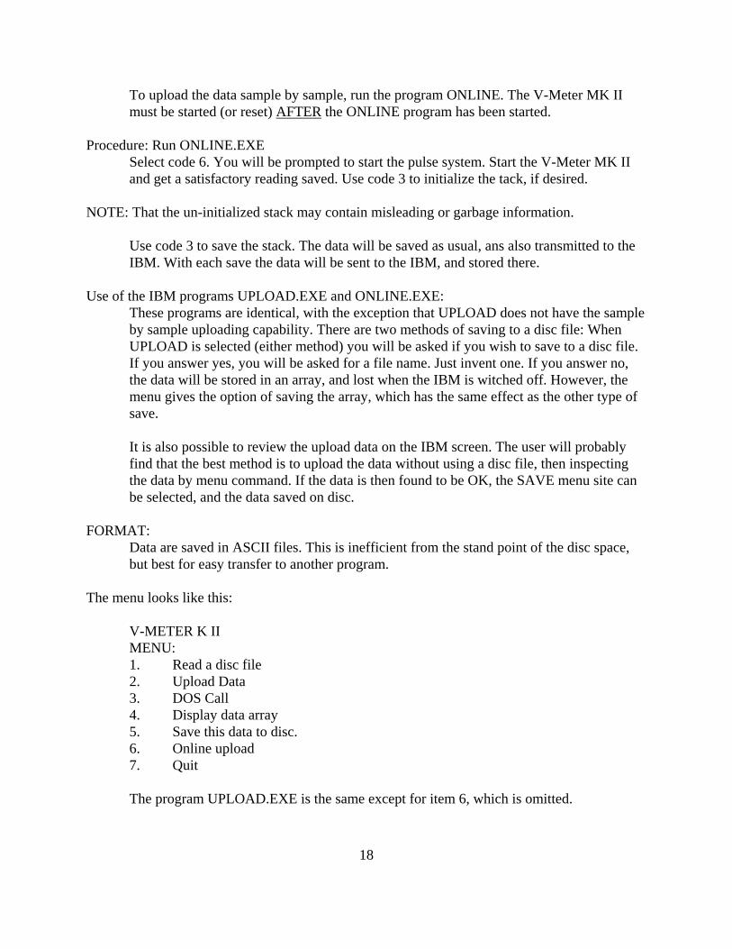
The menu looks like this:

V-METER K II MENU: 1. Read a disc file 2. Upload Data 3. DOS Call 4. Display data array 5. Save this data to disc. 6. Online upload 7. Quit

The program UPLOAD.EXE is the same except for item 6, which is omitted.

19

6) Display mode: See Initialization Item 5 7) Check Stack: This selection allows the operator to scan through the information saved

under the RUN menu. 8) Run: Selection of this item starts the system. ESCAPE stops and returns to the main

menu. 3.5 MENU ITEMS: RUN MENU

1) Run: Same as Run in Main menu.

2) Trace: See Trace in Initialization sequence.

3) Save/Clear: Used to store a reading. An option given is to clear the storage space (stack) for a new start. The data saved are:

A) Distance (In inches) B) Velocity (In inches/second) C) Time (In microseconds) D) Wave type (P (1) or S (0)) E) System (English (0) or Metric (1))

NOTE: The numbers saved are always based on English units. If taken in Metric mode, the conversion has already been accomplished. Memory space is adequate for the storage of 1000 readings.

4) Pulse Rate:

Enables the choice of pulse rates. Options are 1, 3, and 10 pulses/second. Any other choice causes the rate to be approximately 10 pulses/sec.

3.6 FAMILIARIZATION:

A few practice sessions with various cases should remove any mysteries.:

CASE 1: NO HAND HELD TERMINALDisconnect keypad, turn on power.

1) Displays "Contact transducers, then enter." If you wish to re-initialize offset (zero set),

hold the transducers together with couplants and press the "ENTER" switch. If you wish to accept the default value, press "ESC."

20

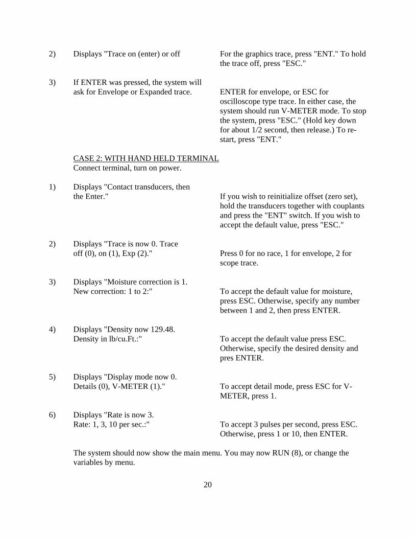
2) Displays "Trace on (enter) or off For the graphics trace, press "ENT." To hold the trace off, press "ESC."

3) If ENTER was pressed, the system will

ask for Envelope or Expanded trace. ENTER for envelope, or ESC for oscilloscope type trace. In either case, the system should run V-METER mode. To stop the system, press "ESC." (Hold key down for about 1/2 second, then release.) To re-start, press "ENT."

CASE 2: WITH HAND HELD TERMINALConnect terminal, turn on power.

1) Displays "Contact transducers, then

the Enter." If you wish to reinitialize offset (zero set), hold the transducers together with couplants and press the "ENT" switch. If you wish to accept the default value, press "ESC."

2) Displays "Trace is now 0. Trace

off (0), on (1), Exp (2)." Press 0 for no race, 1 for envelope, 2 for scope trace.

3) Displays "Moisture correction is 1.

New correction: 1 to 2:" To accept the default value for moisture, press ESC. Otherwise, specify any number between 1 and 2, then press ENTER.

4) Displays "Density now 129.48.

Density in lb/cu.Ft.:" To accept the default value press ESC. Otherwise, specify the desired density and pres ENTER.

5) Displays "Display mode now 0.

Details (0), V-METER (1)." To accept detail mode, press ESC for V-METER, press 1.

6) Displays "Rate is now 3.

Rate: 1, 3, 10 per sec.:" To accept 3 pulses per second, press ESC. Otherwise, press 1 or 10, then ENTER.

The system should now show the main menu. You may now RUN (8), or change the variables by menu.

21

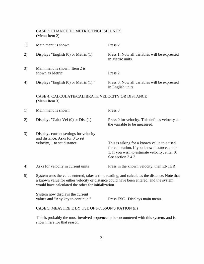
CASE 3: CHANGE TO METRIC/ENGLISH UNITS(Menu Item 2)

1) Main menu is shown. Press 2 2) Displays "English (0) or Metric (1): Press 1. Now all variables will be expressed

in Metric units. 3) Main menu is shown. Item 2 is

shown as Metric Press 2. 4) Displays "English (0) or Metric (1):" Press 0. Now all variables will be expressed

in English units.

CASE 4: CALCULATE/CALIBRATE VELOCITY OR DISTANCE(Menu Item 3)

1) Main menu is shown Press 3 2) Displays "Calc: Vel (0) or Dist (1) Press 0 for velocity. This defines velocity as

the variable to be measured. 3) Displays current settings for velocity

and distance. Asks for 0 to set velocity, 1 to set distance This is asking for a known value to e used

for calibration. If you know distance, enter 1. If you wish to estimate velocity, enter 0. See section 3.4 3.

4) Asks for velocity in current units Press in the known velocity, then ENTER 5) System uses the value entered, takes a time reading, and calculates the distance. Note that

a known value for either velocity or distance could have been entered, and the system would have calculated the other for initialization.

System now displays the current values and "Any key to continue." Press ESC. Displays main menu.

CASE 5: MEASURE E BY USE OF POISSON'S RATION (µ) This is probably the most involved sequence to be encountered with this system, and is shown here for that reason.

22

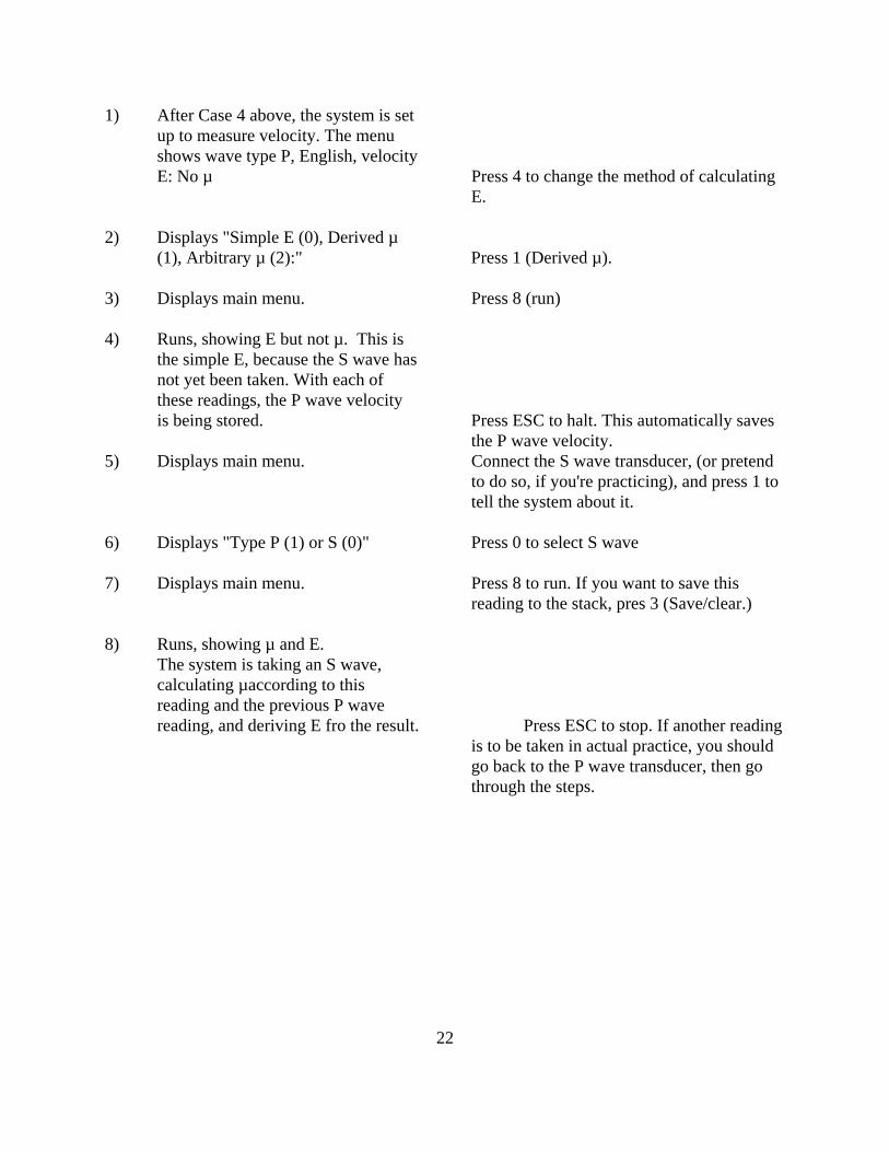
1) After Case 4 above, the system is set up to measure velocity. The menu shows wave type P, English, velocity E: No µ Press 4 to change the method of calculating

E. 2) Displays "Simple E (0), Derived µ

(1), Arbitrary µ (2):" Press 1 (Derived µ). 3) Displays main menu. Press 8 (run) 4) Runs, showing E but not µ. This is

the simple E, because the S wave has not yet been taken. With each of these readings, the P wave velocity is being stored. Press ESC to halt. This automatically saves

the P wave velocity. 5) Displays main menu. Connect the S wave transducer, (or pretend

to do so, if you're practicing), and press 1 to tell the system about it.

6) Displays "Type P (1) or S (0)" Press 0 to select S wave 7) Displays main menu. Press 8 to run. If you want to save this

reading to the stack, pres 3 (Save/clear.) 8) Runs, showing µ and E.

The system is taking an S wave, calculating µaccording to this reading and the previous P wave reading, and deriving E fro the result. Press ESC to stop. If another reading

is to be taken in actual practice, you should go back to the P wave transducer, then go through the steps.

23

3.7 SUMMARY The operation of this system is primarily a matter of observing the interaction. With each menu selection the system asks the appropriate questions, and the operator answers them. If the CASE 5 example has been done successfully, it seems unlikely that the operator will need a separate example of reach menu item. Rather, the best way to gain familiarity with the system is to use it, or simply practice with it, exercising all menu items and observing the action. 3.8 AGENDA 1: Saving for upload: When a series of readings is to be taken, the data are NOT automatically saved on the stack. If data are to be saved, code 3 of the RUN menu must be used for each reading, WHILE THE SYSTEM IS RUNNING. Hold the key down for about 1/2 second, then release. The system will ask "Save (1), no (0), clear stack (5)," Press 1. The system will then continue running. Preparing for use These instructions should be read through before attempting to use the instrument. The front and top panel controls are shown in Fig. 3. PLEASE NOTE: it is essential at all times the battery must be fitted and connected before connecting the instrument to the A.C. mains supply. 3.9 A.C. OPERATION The instrument may be operated from the A.C. mains by plugging the AC/charge cable into the plug on the rear panel and switching the front panel switch to ON. Whenever the instrument is used on the A.C. mains the internal battery will be trickle charged with a constant current. This feature ensures that the battery is maintained in a ready to use state. 3.10 BATTERY OPERATION When the instrument is disconnected fro the mains supply it is only necessary to switch the front panel switch to ON to operate from the battery. When fully charged the battery will operate the instrument for 9 hours. Just prior to the battery discharge end point the front panel red light lights up to indicate the battery low state. The instrument should be turned OFF as over-discharge will damage the battery. 3.11 FULL CHARGING THE INTERNAL BATTERY The discharged battery should be charged at the full rate for 16 hours. Connect the instrument to the mains supply and leave it on for the required time.

24

SECTION IV TAKING PULSE VELOCITY MEASUREMENTS 4.1 TRANSDUCERS Lead Zirconate Titanate ceramics have a relatively low leakage loss and can retain a high voltage charge for a considerable time. A charge can also build up in a ceramic over a period of time due to the crystals being subjected to vibrations during transport. Care should be exercised when handling the coaxial plug prior to connecting to the instrument so as to avoid a shock from a charged transducer. 4.2 OFFSET (ZERO SET) Apply a smear of grease to the transducer faces and press the transducers firmly face to face. The V-Meter Mk II is highly stable and it is not necessary to make frequent checks. Press the switch marked "ENT." 4.3 COUPLANT It is essential in all ultrasonic tests to use some form of couplant between the faces of the transducers and the material under test. Failure to do so will result in a loss of signal due to inadequate acoustical coupling. Silicone grease, medium bearing grease or liquid soap provide good coupling when used on concrete or other materials having smooth surfaces. For rougher surfaces, water pump grease or thick petroleum jelly is recommended. 4.4 PLACING THE TRANSDUCERS It is possible to take measurements of pulse velocity by placing the transducers in three alternative positions: a. Direct transmission with transducers on opposite faces of the material. b. Semi-direct transmission with transducers on adjacent faces. c. Indirect or surface transmission with the transducers on the same face. Method a. Is the most sensitive method as the receiving transducer will receive maximum

energy from the transmitted pulse. Method b. Is the next preferred method and c. should be used only when it is impossible to

get to two faces of the material being tested. The received amplitude of the C

25

method, for the same path length, is only about 2% of that received when using the method a.

4.5 PULSE VELOCITY Having determined the method of transducer placement, make careful measurements of the path length L. Apply couplant to the faces of the transducers and press hard onto the material under test. Do not move the transducers while a reading is being taken as this can generate noise signals and errors in measurement. The pulse velocity is given by: v = L/T where T is the transit time. It is advisable, when using very long leads, to prevent the two leads from coming into close contact with each other when transit time measurement are being made. If this is not done it is possible for the receiver lead to pick up unwanted signals from the transmitter lead resulting in an incorrect display of transit time. Such incorrect displays are readily detected by their instability and the fault may be remedied by separating the leads.

SECTION V SYSTEM DESCRIPTION The V-Meter Mk II generates an ultrasonic pulse in the transmitting transducer and measures the transmission time taken by the pulse to pass from the transmitter to the receiving transducer.

26

27

The system can be conveniently divided into four parts:

1. High voltage and pulse generator 2. CPU with E-prom ram and memory 3. Receiving amplifier 4. Master clock, ADC and display

5.1 PULSE GENERATOR The Pulse Generator comprises a high voltage power unit and a high voltage transistor. The capacitance of the transmitting transducer is charged to a potential of 1.2kV or 500V as selected by the switch on the top panel. This capacitance is then rapidly discharged through a transistor triggered by the pulse derived from the pulse selected by the PRF menu. The repetition frequencies are controlled by CPU. Discharging the capacitance causes the transmitter to be shock excited and so produce a train of longitudinal vibrations at its own natural frequency. 5.2 CPU The central processing unit controls all the functions, calculations, E-prom RAM and memory. 5.3 RECEIVER AMPLIFIER After transmission through the material under test the ultrasonic pulse is converted to an electrical signal in the receiving transducer. The received signal is amplified and shaped to produce a steeply rising "STOP" pulse coincident with the onset of the leading edge of the received signal waveform. 5.4 MASTER CLOCK, ADC AND DISPLAY A 10 MHz quartz crystal oscillator module generates the timing pulses for the 0.1 micro sec unit. The 10 MHz pulses are also applied to dividers to produce timing pulses as required. Analog signals are applied to ADC to convert to digital to put into the CPU and CPU output to the display.

28

SECTION IV TESTING CONCRETE As stated in Section 1 of this Manual, the measurement of the velocity of ultrasonic pulses as a means of testing materials was originally developed for assessing the quality and condition of concrete and the V-Meter Mk II will undoubtedly be used predominately for this purpose. This Section is therefore included to provide the user with some guidance in this field of use. 6.1 APPLICATIONS The pulse velocity method of testing may be applied to the testing of plain, reinforced and prestressed concrete whether it is precast or cast in site. The measurement of pulse velocity may be used to determine:

a) the homogeneity of the concrete,

b) the presence of voids, cracks or other imperfections,

c) changes in the concrete which may occur with time (i.e. due to the cement hydration) or through the action of fire, frost r chemical attack,

d) the quality of the concrete in relation to specified standard requirements, which

generally refer to its strength. 6.2 ACCURACY In most of the applications it is necessary to measure the pulse velocity to a high degree of accuracy since relatively small changes in pulse velocity usually reflect relatively large changes in the condition of the concrete. For this reason it is important that care be taken to obtain the highest possible accuracy of both the transit time and the path length measurements since the pulse velocity measurement depends on both of these. It is desirable to measure pulse velocity to within an accuracy of ±1%. When such accuracy of path length measurement is difficult or impossible, an estimate of the limits of accuracy of the actual measurements should be recorded with the results so that the reliability of the pulse velocity measurements can be assessed. 6.3 COUPLING THE TRANSDUCERS WITH THE CONCRETE SURFACE Accuracy of transit time measurement can only be assured if good acoustic coupling between the transducer face and the concrete surface can be achieved.

29

For a concrete surface formed by casting against steel or smooth timber forms, good coupling can be obtained if the surface is free from dust and grit and covered with a light or medium grease or other suitable couplant. A wet surface presents no problem. If the surface is moderately rough, a stiffer grease should be used but very rough surfaces require more elaborate preparation. In such cases the surface should be ground flat over an area large enough to accommodate the transducer face or this area may be filled to a level smooth surface with a minimum thickness of a suitable material such as Plaster or Paris, cement mortar or epoxy resin, a suitable time being allowed to elapse for the filling material to harden. If the value of the transit time displayed remains constant to within ±1% when the transducers are applied and reapplied to the concrete surface, it is a good indication that satisfactory coupling has been achieved. 6.4 CHOICE OF TRANSDUCER ARRANGEMENT Figure 1 shows three alternative arrangements for the transducers when testing concrete. Whenever possible, the direct transmission arrangement should be used. This will give maximum sensitivity and provide a well defined path length. It is, however, sometimes required to examine the concrete by using diagonal paths and semi-direct arrangements are suitable for these.

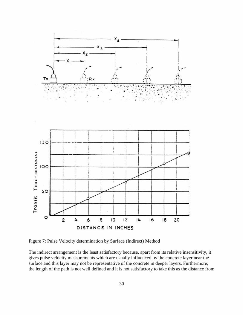
Figure 7: Pulse Velocity determination by Surface (Indirect) Method The indirect arrangement is the least satisfactory because, apart from its relative insensitivity, it gives pulse velocity measurements which are usually influenced by the concrete layer near the surface and this layer may not be representative of the concrete in deeper layers. Furthermore, the length of the path is not well defined and it is not satisfactory to take this as the distance from

30

31

center to center of the transducers. Instead, the method shown in Figure 7 should be adopted to determine the effective path length. In this method, the transmitting transducer is placed on a suitable point on the surface and the receiving transducer is placed on the surface at successive positions along a line and the center to center distance is plotted against the transit tie. The slope of the straight line drawn through these points gives the mean pulse velocity at the surface. In general, it will be found that the pulse velocity determined by the indirect method of testing will be lower than that using the direct method. If it is possible to employ both methods of measurement than a relationship may be established between them and a correction factor derived. When it is not possible to use the direct method an approximate value for Vo may be obtained as follows:

VD = 1.05 V1 where VD is the pulse velocity obtained using the direct method

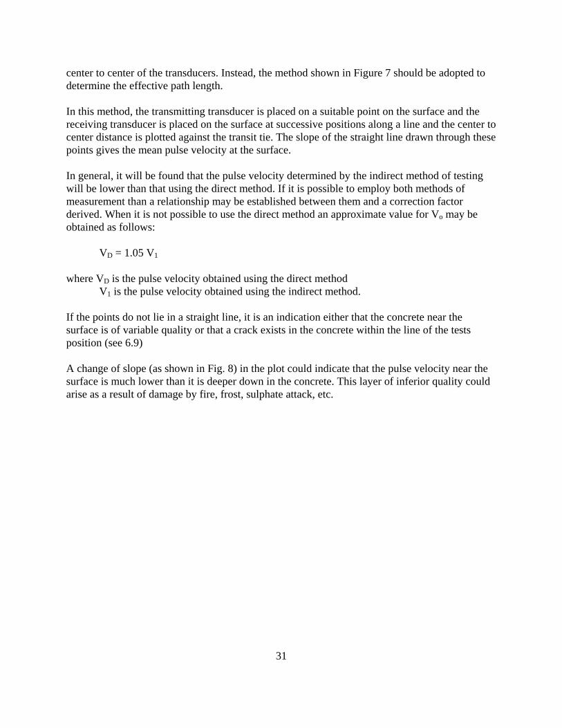
V1 is the pulse velocity obtained using the indirect method. If the points do not lie in a straight line, it is an indication either that the concrete near the surface is of variable quality or that a crack exists in the concrete within the line of the tests position (see 6.9) A change of slope (as shown in Fig. 8) in the plot could indicate that the pulse velocity near the surface is much lower than it is deeper down in the concrete. This layer of inferior quality could arise as a result of damage by fire, frost, sulphate attack, etc.

Fig. 8: Damaged surface layer depth determination by the indirect method. For transducer separation distances up to Xo the pulse travels through the affected surface layer and the slope of the line gives the pulse velocity in this layer. Beyond Xo the pulse has travelled along the surface of the underlying sound concrete and the slope of the line beyond Xo gives the higher velocity in the sound concrete. The thickness of the affected surface layer may be estimated as follows:

32

33

where Vd is the pulse velocity in the damaged concrete (in ft/sec)

Vs is the pulse velocity in the underlying sound concrete (in ft/sec)

t is the thickness of the layer of damaged concrete (in inches)

Xo is the distance at which the change of slope occurs (in inches) 6.5 INFLUENCE OF TEST CONDITIONS The pulse velocity in concrete may be influenced by:

a) path length, b) lateral dimensions of the specimen tested, c) presence of reinforcing steel, or

d) moisture content of the concrete.

The influence of path length will be negligible provided it is not less than 4 inches when .75 inches size aggregate is used or not less than 6 inches for 1.5 inches size aggregate. Pulse velocity will not be influenced by the shape of the specimen provided its least lateral dimension (i.e. its dimension measured at right angles to the pulse path) is not less than the wavelength of the pulse vibrations. For pulses of 50 kHz frequency, this corresponds to a least lateral dimension of about 3 inches. Otherwise the pulse velocity may be reduced and the results of pulse velocity measurements should be used with caution (see Table 1).

Fig. 9: Influence of steel reinforcement on pulse velocity. Bars at right angles to path. 34

35

The temperature of the concrete has been found to have no significant effect on pulse velocity over the range from 5° to 30°C so that, except for abnormally extreme temperatures, influence may be disregarded (see Table 2). Table 1. Effect of specimen dimensions on pulse transmission

Table 2. Effect of temperature on pulse transmission

Pulse velocity in concrete (in ft/s) Correction to the velocity

vc=12000 vc=13500 Vc=15000

Transducer frequency

Minimum permissible lateral specimen dimension

Temperature Air-dried

concrete Water-saturated concrete

kHz 24 54 82 150

Inches

6 2.6 1.8 1.0

Inches

6.8 3

2.0 1.1

Inches

7.5 3.3 2.2 1.2

˚C 60 40 20 0 -4

% +5 +2 0

-0.5 -1.5

% +4

+1.7 0 -1

-7.5 The velocity of pulses in a steel bar is generally higher than they are in concrete. For this reason, pulse velocity measurements made in the vicinity of reinforcing steel may be high and not representative of the concrete since the V-Meter Mk II indicates the tie for the first pulse to reach the receiving transducer. The influence of the reinforcement is generally very small if the bars run in the direction at right angles to the pulse path and the quantity of steel is small in relations to the path length. Figure 9 shows how this influence may be allowed for when the bar diameter lies directly along the pulse path. If the ration Ls/L is known, the measured pulse velocity may be corrected by multiplying it by the correction factor corresponding to the ratio and the quality of the concrete. It is however preferable to avoid such a path arrangement and to choose a path which is not in a direct line with the bar diameters.

36

37

When the steel bars lie in a direction parallel to the pulse path, the influence of the steel may be more difficult to avoid as can be seen from Figure 10. It is, however, not easy to make reliable corrections for the influence of the steel and the correction factors given in Figure 10 should be regarded as approximate only. It is generally found that these values represent an upper limit of the steel influence. Again, it is advisable to choose pulse paths which avoid the influence of the steel as far as possible. The moisture content of concrete can have a small but significant influence on the pulse velocity. In general, the velocity is increased with increased moisture content, the influence being more marked for lower quality concrete. The pulse velocity of saturated concrete may be up to 2% higher than in dry concrete of the same composition and quality, although this figure is likely to be lower for high strength concrete. When pulse velocity measurements are made on concrete as a quality check, a contractor may be encouraged to keep the concrete wet for as long as possible in order to achieve an enhanced value of pulse velocity. This is generally an advantage since it provides an incentive for good curing practice. 6.6 HOMOGENEITY OF THE CONCRETE Measurement of pulse velocities at points on a regular grid on the surface of a concrete structure provides a reliable method of assessing the homogeneity of the concrete. The size of the grid chosen will depend on the size of the structure and the amount of variability encountered. It is useful to plot a diagram of pulse velocity contours from the results obtained since this gives a clear picture of the extent of variations. It should be appreciated that the path length can influence the extent of the variations recorded because the pulse velocity measurements correspond to the average quality of the concrete along the line of the pulse path and the size of concrete sample tested at each measurement is directly related to the path length. 6.7 DETECTION OF DEFECTS When an ultrasonic pulse traveling through concrete meets a concrete-air interface, there is a negligible transmission of energy across this interface so that any air filled crack or void lying directly between the transducers will obstruct the direct beam of ultrasound when the void has a projected area larger than the area of the transducer faces. The first pulse to arrive at the receiving transducer will have been diffracted around the periphery of the defect and the transit time will be longer than in similar concrete with no defect. It is sometimes possible to make use of this effect for locating flaws, etc. but it should be appreciated that small defects often have little or no effect on transmission times.

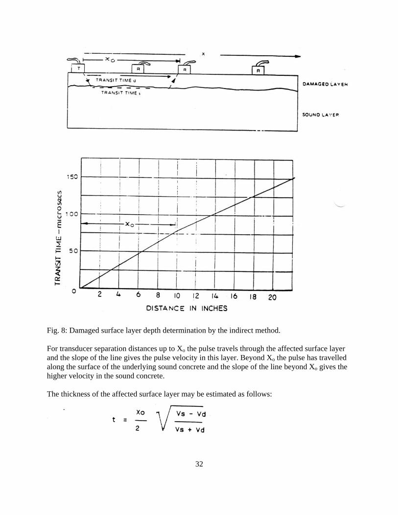
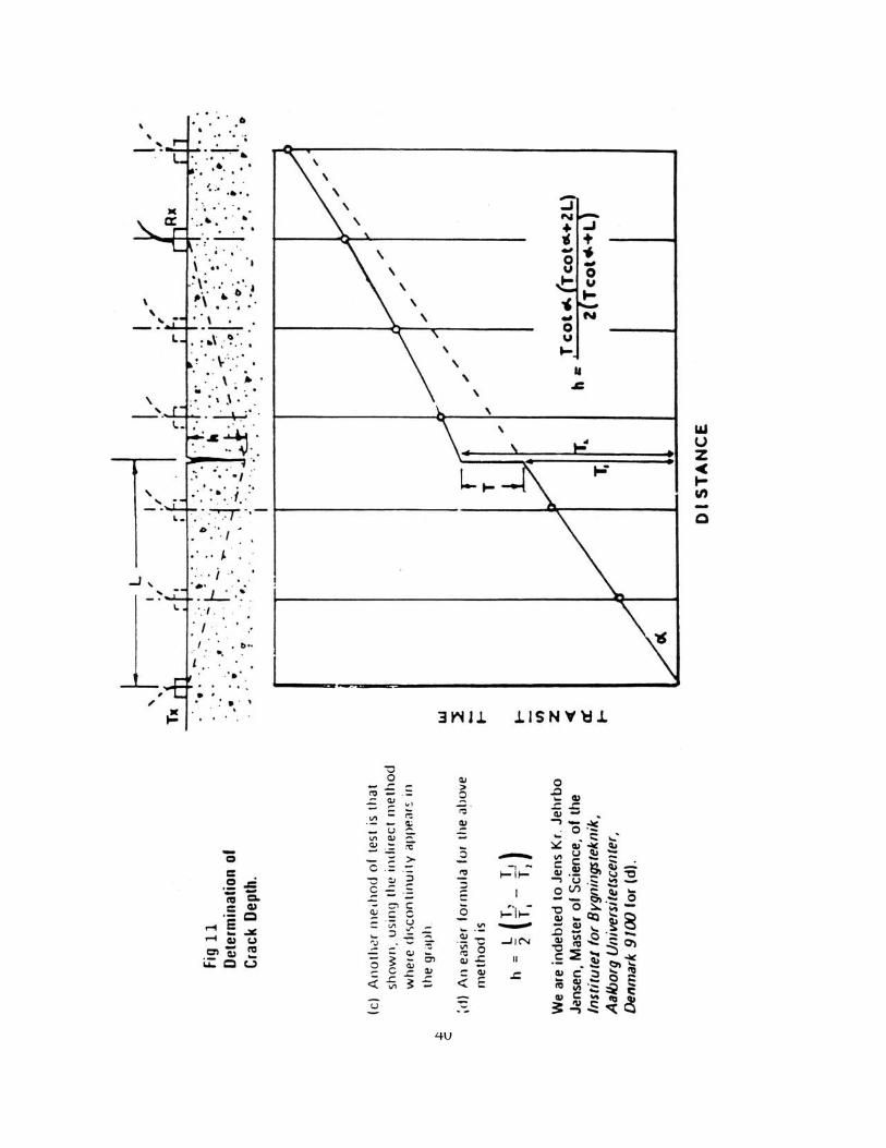
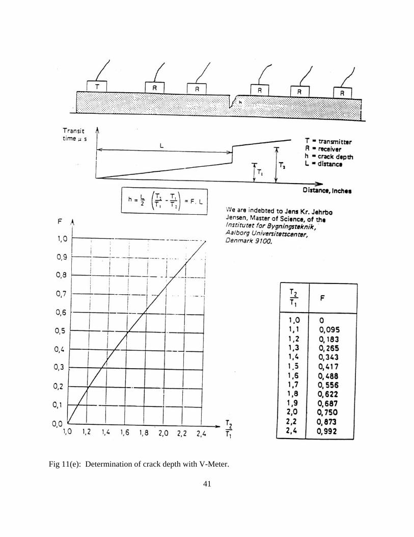
6.8 DETECTION OF LARGE VOIDS OR CAVITIES A large cavity may be detected by measuring the transit times of pulses passing between the transducers when they are placed in suitable positions so that the cavity lies in the direct path between them. The size and position of such cavities may be estimated by assuming that the pulses pass along the shortest path between the transducers and around the cavity. Such estimates are more reliable if the cavity has a well defined boundary surrounded by uniformly dense concrete. If the projected area of the cavity is smaller than the diameter of the transducers, the cavity cannot be detected by transit time measurement alone. 6.9 ESTIMATING THE DEPTH OF SURFACE CRACKS An estimate of the depth of a crack visible at the surface can be obtained by measuring the transit times across the crack for two different arrangements of the transducers placed on the surface. One suitable arrangement is shown in Fig. 11 (a) in which the transmitting and receiving transducers are placed on opposite sides of the crack and equidistant from it. Two values of x are chosen, one being twice that of the other, and the transit times corresponding to these are measured. The equation given in Fig. 11 (a) is derived by assuming that the plane of the crack is perpendicular to the concrete surface and that the concrete in the vicinity of the crack is of reasonably uniform quality.

a) Estimation of crack depth. Crack perpendicular to concrete surface.

Let first value of x chosen be X1 and second value be 2 X1 and the transit times corresponding to these be T1 and T2 respectively, then

38

b) Check on inclination of crack

Place both transducers near to the crack and on opposite sides of it. Move one of them away from crack. If the transit time decreases this indicates that the crack slopes towards the direction in which the transducer was moved.

39

40

41

Fig 11(e): Determination of crack depth with V-Meter.

42

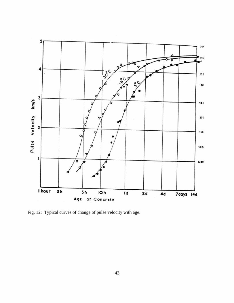
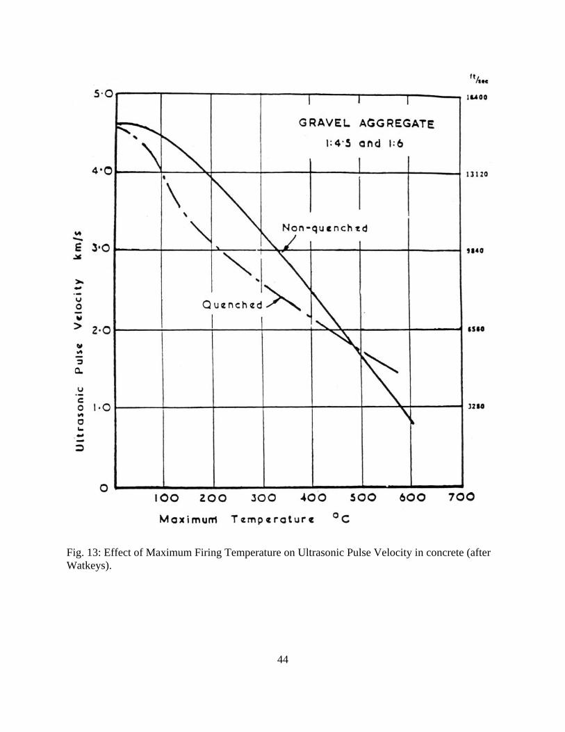
A check may be made to assess whether the crack is lying in a plane perpendicular to the surface by placing both transducers near to the crack and moving one of them as in Fig. 11 (b) It is important that the distance x be measured accurately and that very good coupling is developed between the transducers and the concrete surface. The method is valid provided the crack is not filled with water. 6.10 MONITORING CHANGES IN CONCRETE WITH TIME Changes occurring in the structure of concrete with time caused by either hydration (which increases strength) or by an aggressive environment, such as frost, or sulphates, may be determined by repeated measurements of pulse velocity at different times. Changes in pulse velocity are indicative of changes in strength and their measurement can be made over progressive periods of time on the same test piece or concrete product. This facility is particularly useful for following the hardening process during the first two days after casting and it is sometimes possible to take measurement through formwork before it is removed at very early ages. Figure 12 shows some typical experimental results of pulse velocity measurements at early ages. This has a useful application for determining when formwork can be removed or when prestressing operations can proceed. (See also Section VI, Figure 18.) Figure 12: Typical curves of change of pulse velocity with age. 6.11 ESTIMATION OF STRENGTH AFTER FIRE DAMAGE Pulse velocity measurements may be used to assess the extent of damages to concrete after a fire. Figures 13 and 14 shows some typical results as obtained by Watkeys who showed that a good correlation existed between the maximum temperature reached by the concrete and the percentage reduction in pulse velocity due to heating. He also showed that a useful correlation could be obtained to estimate the residual crushing strength of the concrete after heating from pulse velocity tests. In Figure 13, the two curves are for two sets of concrete specimens which had been heated and cooled down either by spraying with water (quenched) or by loss of heat slowly in air (unquenched). Figure 14 shoes that, for a given residual strength, the pulse velocity was apparently less than that for undamaged concrete. These results were for concrete made with gravel aggregate and are typical of normal concrete although no information is available regarding the effect of different types of aggregate on the correlations.

Fig. 12: Typical curves of change of pulse velocity with age.

43

Fig. 13: Effect of Maximum Firing Temperature on Ultrasonic Pulse Velocity in concrete (after Watkeys).

44

Fig. 14: Curve relating residual strength with pulse velocity for concrete damaged by fire. 6.12 ESTIMATION OF STRENGTH Concrete quality is generally assessed by measuring its cylinder (or cube) crushing strength. It has been found that there is no simple correlation between cylinder strength and pulse velocity but the correlation is affected by:

type of aggregate, aggregate/cement ratio age of concrete

45

size and grading of aggregate curing conditions

Fuller details of the effects of these may be found in references and S. Garg and S. Shah developed a prediction equation. fc = -6364.74 + 15089.27 (vel.) -016 - 221.05 (cem. ) -068 - .065

(Sand) 1.75 - .815 x 10 -7 (agg)3.5 -0.95 x 10-9

(Wtr)5.0

in which Vel.: Velocity in ft/sec. Cem.: Cement lbs. cub. yd. Sand: Sand lbs./cub. yd. Agg.: Aggregate obs./cu. yd. Wtr.: Water lbs/cub. yd. fc: in psi with the r = 0.966

In practice, if pulse velocity results are to be expressed as equivalent cylinder strengths, it is preferable to calibrate the particular concrete used by making a series of test specimens with materials and mix proportions the same as the specified concrete but having a range of strengths. The pulse velocity is measured for each specimen which is then tested to failure by crushing. The range of strength may be obtained either by varying the age of the concrete at test or by introducing a range of water-cement ratios. The curve relating cylinder strength to pulse velocity is not likely to be the same for these two methods of varying strength but the particular method chosen should be appropriate to the test purpose required. If strength monitoring with time is to be carried out, the calibration curve is best obtained by varying the age but a check on quality at a particular age would require the correlation to be obtained by varying the water-cement ratio.

46

The Correlation graph below was obtained by measuring pulse velocity and equivalent cube strength of beams as shown above.

Fig. 15: Typical Strength, Velocity Correlations for concrete.

47

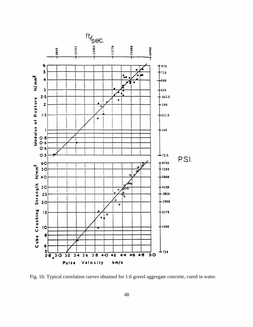
Fig. 16: Typical correlation curves obtained for 1:6 gravel aggregate concrete, cured in water. 48

49

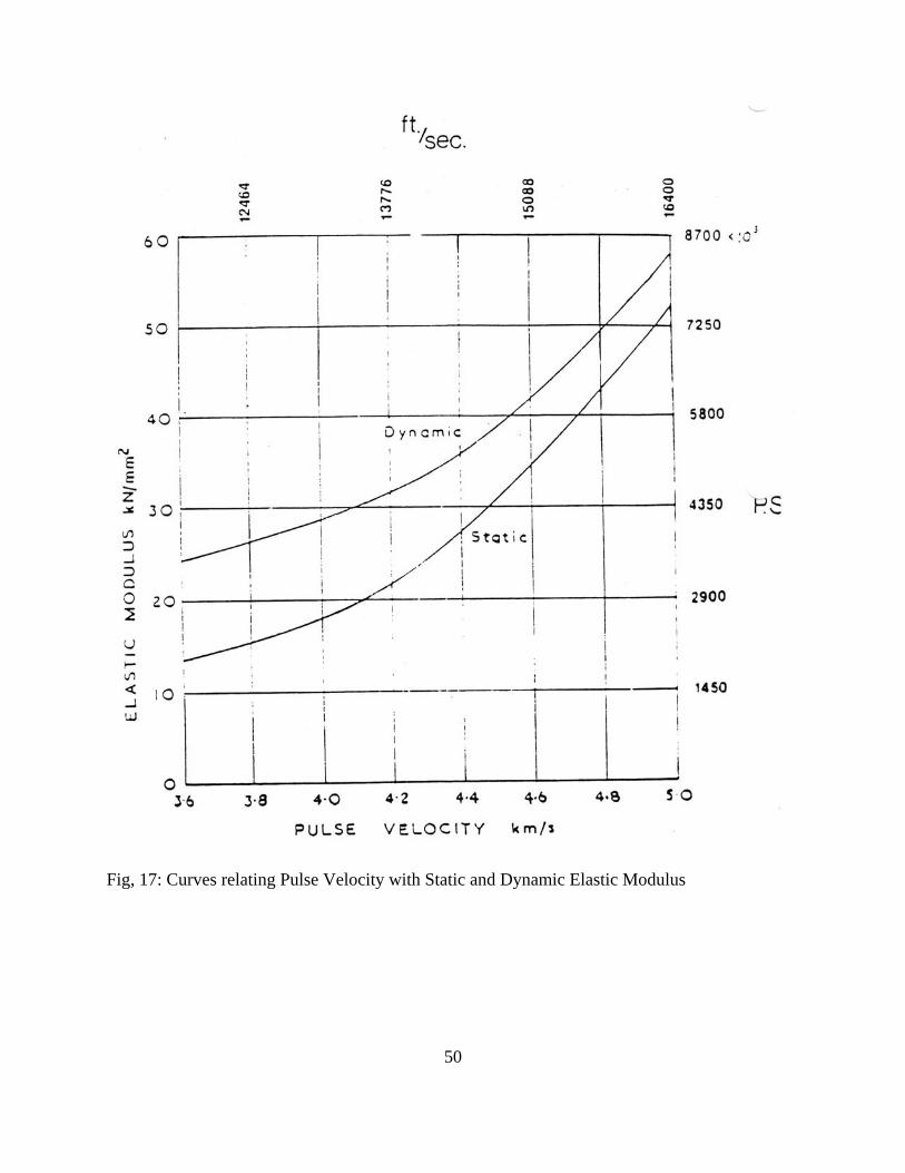
Although such correlations can be obtained from tests on cylinders, it is preferred in Europe to use beams such as those used for testing the modulus of rupture of concrete. These beams are 500 mm long and more accurate value of pulse velocity is obtained by using the long axis as the pulse path. After testing ultrasonically, the beams are tested in flexure to determine the modules of rupture and the broken halves tested by crushing to measure the equivalent cube strength. Figure 15 shows a typical curve obtained for a concrete made with river gravel aggregate and calibrated by using beams. When testing the concrete in a structure, it would be unreasonable to expect the value of the cylinder strength estimated from pulse velocity measurements to be the same as that specified for the control cylinders made on the site since the design of concrete structures takes into account the fact that cylinder are likely to be of higher strength than the concrete in the structure which it represents. A suitable tolerance is therefore required to allow for this. This subject is discussed more fully in other reference. Figure 16 shows further typical correlation curves including one for modulus of rupture and these are for a 1:6 mix using gravel aggregate concrete. Instead of expressing the strength in terms of cylinder strength, it is preferable to obtain a direct correlation between the strength of a structural member and the pulse velocity whenever this is possible. Such correlation can often be readily applied to precast units and it is possible to obtain a curve relating pulse velocity with the appropriate mechanical test (such as bending) for the unit. 6.13 ESTIMATION OF ELASTIC MODULUS The estimating of elastic modulus is less complicated than the estimation of strength and it has been found that a single curve may be used to relate pulse velocity to elastic modulus for a wide range of different aggregates, including concrete made with lightweight aggregate (see Table 3).

Fig, 17: Curves relating Pulse Velocity with Static and Dynamic Elastic Modulus

50

6.14 DETERMINATION OF THE DYNAMIC MODULUS OF ELASTICITY AND

DYNAMIC POISSON'S RATIO The relationship between elastic constants and the velocity of an ultrasonic compressional wave pulse in an isotropic elastic medium of infinite dimension is given by: Ed = ∆V2 (1+µ)(1-2µ)/(1-µ) where Ed = the dynamic elastic modules (psi).

µ = The dynamic Poisson's ratio. ∆= the density (lbs./cu ft) V = the compressional pulse velocity (ft /sec).

Also, the dynamic modulus of elasticity Ed, found from the longitudinal resonant frequency test (see ASTMC 215), is given by:

Ed = 4fL 2L2 ∆

51

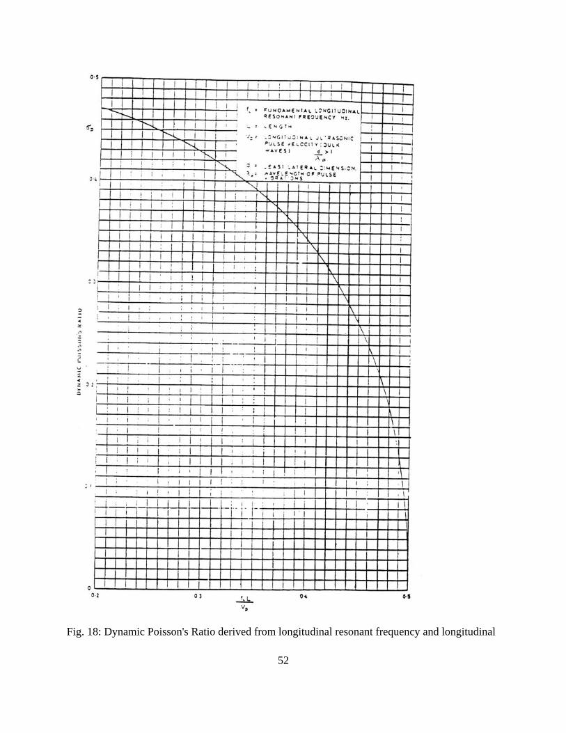
Fig. 18: Dynamic Poisson's Ratio derived from longitudinal resonant frequency and longitudinal 52

53

pulse velocity. where fL = The fundamental longitudinal resonant frequency (hz)

L = the length (in) p = bulk density (lbs/cu ft)

Combining equations (1) and (2) gives: (1+µ)(1-2µ)/(1-µ) = 2fLL/V The value of dynamic Poisson's ratio µ may be determined from Table 4 or obtained from Fig. 18. The value of the longitudinal resonant frequency fL2 of laboratory prisms, may be obtained by use of the "E-Meter" electrodynamic resonant frequency test equipment which fully complies with the ASTMC 215-85 standards.

Table 4. Values of dynamic Poisson’s ratio

fLL V

µ

0.257 0.342 0.395 0.431 0.456 0.474 0.487 0.494 0.499

0.45 0.40 0.35 0.30 0.25 0.20 0.15 0.10 0.05

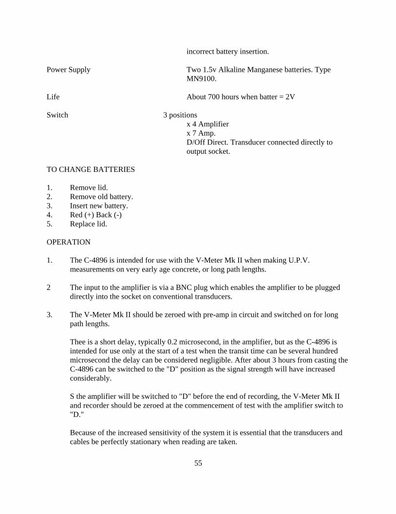
SECTION VII ADDITIONAL ACCESSORIES FOR USE WITH THE V-METER MK II 7.1 LONGITUDINAL (P-WAVE) TRANSDUCERS Several different frequency transducers are available for specific applications other than the standard 54 Khz and 150 kHz i.e. 24 kHz, 37 kHz, 84 kHz, 500 kHz etc. 7.2. SHEAR WAVE TRANSDUCER Shear wave transducers with approximately 100 kHz frequency are available to measure and calculate Poisson's ratio. 7.3 DIFFERENT SHAPE TRANSDUCERS Transducers with different shapes are available other than standard flat faced cylindrical configurations for example, exponential transducers for very rough surfaces or wheel transducers for fast scanning of flat surface. 7.4 PRE-AMPLIFIER TYPE C-4896 - Fig. 19

Voltage gain x4/x7 Frequency response 100 Hz-240kHz "with 200 ft. cable on output - 100

Hz - 60kHz" Amplifier delay Typically 0.2 microsec. Amplifier noise < 20 micro V

54

Protection Input and output fully protected. Protected against

55

incorrect battery insertion. Power Supply Two 1.5v Alkaline Manganese batteries. Type

MN9100. Life About 700 hours when batter = 2V Switch 3 positions

x 4 Amplifier x 7 Amp. D/Off Direct. Transducer connected directly to output socket.

TO CHANGE BATTERIES 1. Remove lid. 2. Remove old battery. 3. Insert new battery. 4. Red (+) Back (-) 5. Replace lid. OPERATION 1. The C-4896 is intended for use with the V-Meter Mk II when making U.P.V.

measurements on very early age concrete, or long path lengths. 2 The input to the amplifier is via a BNC plug which enables the amplifier to be plugged

directly into the socket on conventional transducers. 3. The V-Meter Mk II should be zeroed with pre-amp in circuit and switched on for long

path lengths.

Thee is a short delay, typically 0.2 microsecond, in the amplifier, but as the C-4896 is intended for use only at the start of a test when the transit time can be several hundred microsecond the delay can be considered negligible. After about 3 hours from casting the C-4896 can be switched to the "D" position as the signal strength will have increased considerably.

S the amplifier will be switched to "D" before the end of recording, the V-Meter Mk II and recorder should be zeroed at the commencement of test with the amplifier switch to "D."

Because of the increased sensitivity of the system it is essential that the transducers and cables be perfectly stationary when reading are taken.

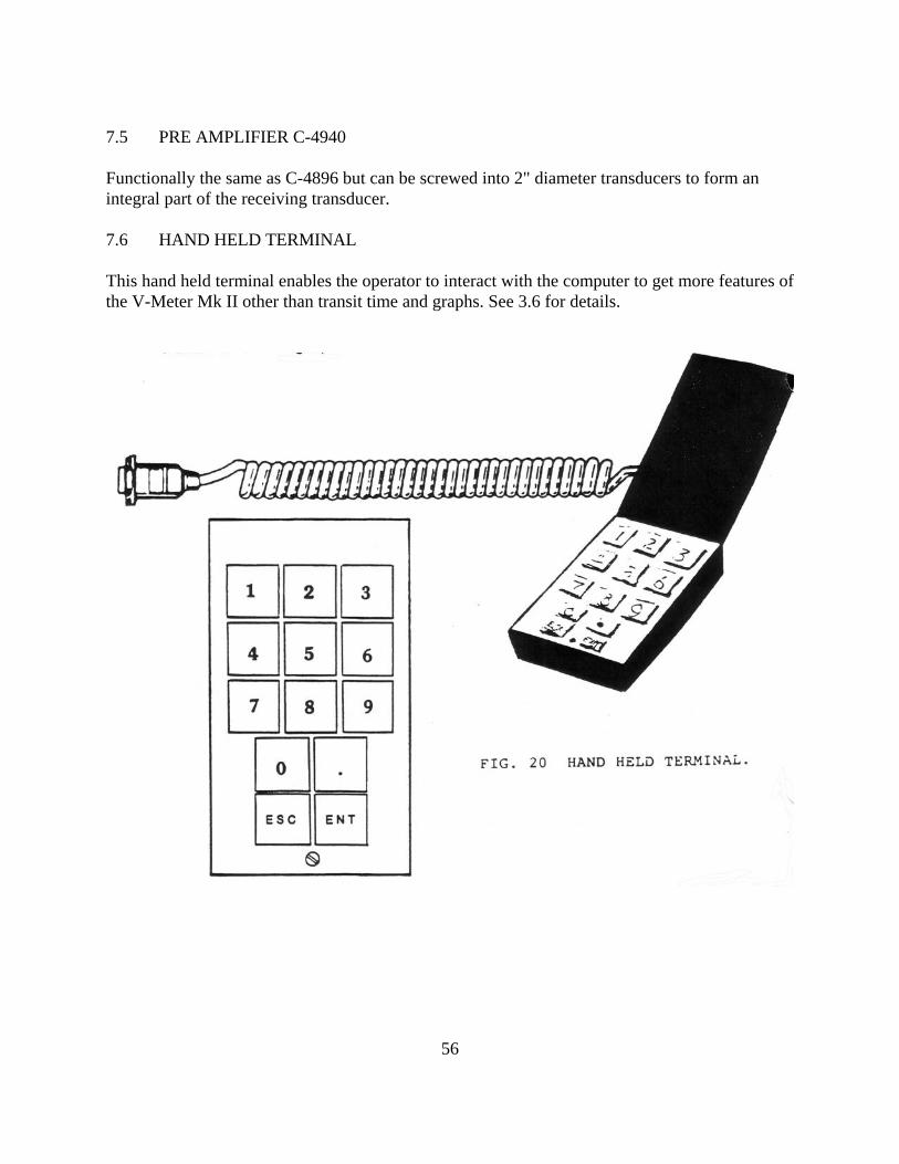
7.5 PRE AMPLIFIER C-4940 Functionally the same as C-4896 but can be screwed into 2" diameter transducers to form an integral part of the receiving transducer. 7.6 HAND HELD TERMINAL This hand held terminal enables the operator to interact with the computer to get more features of the V-Meter Mk II other than transit time and graphs. See 3.6 for details.

56

57

REFERENCES F-6063 Ultrasonic Testing of Concrete. The use of the V-Meter. General Paper. James

Instruments, Inc. V-103 Pulse Velocities Recorded on Sectioned Pieces of Wooden Utility Poles. R.A. Muenow,

1966. V-107 Non-Destructive Testing of Construction Materials. James Electronics. V-108 Report on Pulse Velocity Measurement for the Garage Structure - First National

Building, Detroit, Michigan. R.A. Muenow, 1965. V-117 The Ultrasonic Nondestructive Evaluation of Wood Utility Poles, Wood and Concrete

Railway Ties and Trestles, and Other Similar Structures. R.A. Muenow, 1966. V-118 Pulse Velocity - A method of Evaluating and Inspecting Large and Small Hydro-Electric

Structures. R.A. Muenow, 1966. V-119 The Evaluation of a Reinforced Concrete Frame Building by Pulse Velocity Methods.

R.A. Muenow, 1966. V-122 The Determination of fracture Healing by Measurement of Sound Velocity Across the

Fracture Site. Siegel/Anast/Fields, 1958. V-124 Fire Resistance of a Reinforced Concrete Building. Observations Recorded After the

First and Repair of Damage. Brice/Chefdeville, 1959. V-127 Evaluation of Wooden Elements Taken from Various Railroad Structures. James, 1966. V-129 The Use of Velocity Measurements on Living Trees. James, 1966. V-130 Caisson Investigations. James, 1966. V-131 The Correlation of Compressive Strength with the Velocity of Sound Propagation

Through Concrete. R.A. Muenow, 1967. V-138 Caissons Inspection at Hot Strip Mill for Youngstown Sheet & Tube Company,

Hammond, Indiana. R.A. Muenow, 1966. V-143 Evaluation of Prestressed Concrete Beam. Richard A. Muenow. V-144 Inspection of Solid Fuel Elements. R.A. Muenow, 1967.

58

V-146 A Sonic Method to Determine Pavement Thickness. R.A. Muenow, 1963. V-150 Experimental Study of Pulse Velocities in Compacted Soils. Highway Research Record,

James. V-153 Standard Method of Test for Fundamental Transverse, Longitudinal, and Torsional

Frequencies of Concrete Specimens. American Society for Testing & Materials, C-215 V-154 Standard Method of Test for Pulse Velocity Through Concrete. ASTM, C-597 V-155 Mechanical Behavior of Concrete Examined by Ultrasonic Measurements.

Shah/Chandra, 1970. V-156 Concrete Research news. University College, University of London. V-157 Influence of Binary Aggregate Proportions Upon Some Concrete Properties. Daniel N.

Nwokoye. V-158 Ultrasonic Pulse Velocity Measurements Through Fresh Concrete. D.W.E. Smit. V-159 The Influence of Fibres Upon Crack Development in Reinforced Concrete Subject of

Uniaxial Tension. M.A. Sumarral / R.H. Elvery, 1974. V-160 FPL's Defectoscope; Experimental Device to Increase Lumber Yields. Kent A.

McDonald. V-161 Ultrasonic Location of Defects in Softwood Lumber. Kent A. McDonald, 1973. V-162 Locating Lumber Defects by Ultrasonics. McDonald/Bulgrin, 1969. V-163 Stress Wave Speed and MOE of Sweetgum Ranging from 150 to 15% MC. C.C.

Gerhards, 1975. V-164 Non-Destructive Prediction of Concrete Compressive Strength, Seals/Anderson, 1976. V-165 High Strength Gunite in the Repair of Fire Damage. Wilce, 1974. V-166 Non-Destructive Testing of Floor Slabs. Tomset, 1973. V-167 The Strength Characterization of Kraft Paper by Means of Sonic Pulse Velocity

Measurement. Jackson/Gavelin, 1967. V-168 Non-Destructive Sonic Measurement of Paper Elasticity. Crever/Taylor, 1965.

59

V0169 Sonic Pulse Propagation in Paperlike Structure. Chattergie, 1969. V-170 Ultrasonic Techniques in Ceramic Research and Testing. Doris/Brough, 1972. V-171 Estimating Strength of Concrete in Structures. Elvery, 1973. V-172 Ultrasonic Testing of Concrete Pipe. James Report, 1974. V-173 Dry Valley Drilling Project, Barrett. V-174 Non-destructive Testing of Concrete. R.H. Elvery/H.A. Forrester, 1971. V-175 Non-destructive Testing of Timber at Washington State University. R.F. Pellerin. V-176 The Strength of In Situ Concrete. D.O. Maynard/S.G. Davis, 1974. V-177 Ultrasonic Testing for Large Sections. Tomsett, 1973. V-178 A Review of the Non-destructive Testing of Concrete. R. Jones. V-179 Ultrasonic Inspection of Reinforced Concrete Flexural Members. R. Elvery /N. Din. V-180 Non-destructive Testing of Concrete and its Relationship to Specifications. R. Elvery,

1971. V-181 On the Site. J.H. Bungey, 1974. V-182 Site Testing of Concrete. Henry N. Tomsett, 1976. V-183 Changes in the Velocity of Ultrasound in Meat during Freezing. C. Miles/C,. Cutting,

1974. V-184 Final Report on the Evaluation of the Graphite Form in Ferritic Ductile Iron by

Ultrasonic and Sonic Testing, and the Effect of Graphite Form on Mechanical Properties. P. Emerson/W. Simmons.

V-185 Strength Assessment of Timber for Glued Laminated Beams. R. Elvery / D. Nwokoye. V-187 Cement and Concrete Association Report for 1974. V-188 Recommendations for Non-destructive Methods of Test for Concrete and Part 5:

Measurement of the Velocity of Ultrasonic Pulses in Concrete. British Standards Institute, 1974.

60

V-189 Report on the Failure of Roof Beams at Sir John Cass' Foundation and Red Coat Church of England Secondary School, Stepney. S.C. Bate, 1974.

V-190 Further Notes on Ultrasonic Techniques. W.R. Davis, 1974. V-191 Ultrasonic Control. V-194 Further Investigations Into the Strength of Concrete in Structures. S.G. Davis. V-195 Nondestructive Testing of Particleboard. R. Pellerin & Chas. Morschauser, 1973. V-196 Ultrasonic Testing of Ceramics and Refractories with James V-Meter. K. Choi, 1978. V-197 Utility Pole Testing, Report on test program with V-Meter. V-198 Past and Future of Concrete Quality Evaluation. Journal of The Construction Division. V.

Ramakrishnan. V-199 Nondestructive Method for Measuring the Electric Anisotropy of Wood using an

Ultrasonic Pulse Technique. I.D.G. Lee V-200 Nondestructive testing of concrete and timber. Institute of Civil Engineers and the British

Natl. Com. For nondestructive testing. V-201 Lumber Defect Detection by Ultrasonics. Forest Service, Madison, Wisconsin V-202 Nondestructive Testing of Wood. College of Engineering Research, Washington State

University. Wm. L. Galligan. V-204 The Ultrasonic Pulse Velocity Method of Test for Concrete in Structures. Cement and

concrete Association. H.N. Tomset, Oct. 1977. V-205 Testing of Wood and Wood Products with Low Frequency Ultrasonics. A Review, .

Choi, 1978. V-207 Assessment Techniques for Graphite Electrodes. John R. Lakin, Fuel, 1978 V-208 An Appraisal of the Ultrasonic Pulse Technique for Detecting Voids in Concrete. H.W.

Chung, University of Hong Kong. V-209 The In Situ Evaluation of Concrete Using Pulse Velocity Differences. H.N. Tomsett,

1978 American Concrete Institute Fall Convention in Houston, Texas. V-210 "The Cylinder Test" Reliable Informer or False Prophet. James M. Shilstone, Sr., FACI

61

President, The Concrete Associates, Inc. 1979 (Ultrasonic Testing) CERAMIC REFERENCES 1. Sonic Testing of Refractories. T.H. Hawisher & C.E. Semler, American Ceramic Society

80th Annual Meeting, Detroit, 1978. 2. Improved Reliability of Fused S1O2 Pouring Tubes for Continuous Casting with

Nondestructive Inspection. M.S. Judd, C.G. Hammersmith, R.L. Wessel & D.M. Scott, American Ceramic Society 81st Annual Meetings, Cincinnati, 1979.

3. Sonic Velocity Measurement on Pouring Pit Refractories. D.S. Whittemore, American

Ceramic Society Annual Meeting, Cincinnati, 1979. 4. Pulse Ultrasonics in Process Control. Bruce Dunsworth and Don Smith. Refractory

Division Fall Meeting, Bedford Spring, PA, 1979. 5. Nondestructive Ultrasonic Testing of fireclay Refractories. L.B. Lawler, R.H. Ross and

E. Ruh, American Ceramic Society 82nd Annual Meeting, Chicago, 1980. 6. Refractory Evaluation with Pulse Ultrasonic. W. Miller, American Ceramic Society 82nd

Annual Meeting, Chicago, 1980. 7. Cordierite Slab. W.C. Mohr, B.E. Dunworth, D.B. McCuen and M.W. Morris, American

Ceramic Society 82nd Annual Meeting, Chicago, 1980. 8. Fracture Energy Testing: Single Bar Determination of WOF and NBT. Merrill Wood,

General Refractories Company, U.S. Refractories Division - Research Center, Baltimore, MD.

9. Sonic Velocity Quality Control of Steel Plant Refractories. Robert O. Russell & Gary D.

Morrow, American Ceramic Society, Ceramic Bulletin, Vol. 63 no. 7, 1984.