VALIDATION OF SOURCE APPROVAL OF HMA SURFACE MIX AGGREGATE Morgan State University The Pennsylvania State University University of Maryland University of Virginia Virginia Polytechnic Institute & State University West Virginia University The Pennsylvania State University The Thomas D. Larson Pennsylvania Transportation Institute Transportation Research Building University Park, PA 16802-4710 Phone: 814-865-1891 Fax: 814-863-3707 www.mautc.psu.edu
Transcript
VALIDATION OF SOURCE APPROVAL OF HMA SURFACE MIX AGGREGATE
Morgan State University The Pennsylvania State University
University of Maryland University of Virginia
Virginia Polytechnic Institute & State University West Virginia University
The Pennsylvania State University The Thomas D. Larson Pennsylvania Transportation Institute
Transportation Research Building University Park, PA 16802-4710 Phone: 814-865-1891 Fax: 814-863-3707
www.mautc.psu.edu
STATE HIGHWAY ADMINISTRATION
RESEARCH REPORT
VALIDATION OF SOURCE APPROVAL OF
HMA SURFACE MIX AGGREGATE
FREDERICK K. WILSON, PHD (PI)
OLUDARE OWOLABI, DSC (CO-PI)
ARTHUR WILLOUGHBY
JAMES WHITNEY II, PHD
MORGAN STATE UNIVERSITY
FINAL REPORT
April 2016
MD-16-SHA/MSU/4-2
Larry Hogan, Governor Boyd K. Rutherford, Lt. Governor
Pete K. Rahn, Secretary Gregory C. Johnson, P.E., Administrator
2
DISCLAIMER The contents of this report reflect the views of the author who is responsible for the facts and the accuracy of the data presented herein. The contents do not necessarily reflect the official views or policies of the Maryland State Highway Administration. This document is disseminated under the sponsorship of the U.S. Department of Transportation, University Transportation Centers program, in the interest of information exchange. The U.S. government assumes no liability for the contents and use thereof. This report does not constitute a standard, specification, or regulation.
2. Government Accession No. 3. Recipient's Catalog No.
4. Title and Subtitle Validation of Source Approval of HMA Surface Mix Aggregate
5. Report Date April 2016
6. Performing Organization Code
7. Author/s Frederick K. Wilson, Oludare Owolabi, Arthur Willoughby, and James Whitney II.
8. Performing Organization Report No.
9. Performing Organization Name and Address Morgan State University 1700 E. Cold Spring Ln. Baltimore, MD 21251
10. Work Unit No. (TRAIS)
11. Contract or Grant No.
SHA/MSU/4-2 12. Sponsoring Organization Name and Address Maryland State Highway Administration Office of Policy & Research 707 North Calvert Street Baltimore MD 21202
13. Type of Report and Period Covered
Final Report 14. Sponsoring Agency Code (7120) STMD- MDOT/SHA
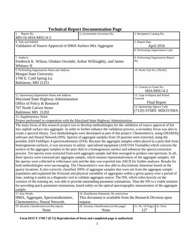
15. Supplementary Notes Project performed in cooperation with the Maryland State Highway Administration. The main focus of this research project was to develop methodologies for the validation of source approval of hot mix asphalt surface mix aggregate. In order to further enhance the validation process, a secondary focus was also to create a spectral library. Two methodologies were developed as part of this project: Chemometrics, using GRAM/IQ software and Neural Network (NN). Spectra of aggregate samples from 19 quarries were extracted, using the portable ASD FieldSpec 4 spectroradiometer (FS4). Because the aggregate samples when placed in a petri dish form heterogeneous surfaces, it was necessary to utilize specialized equipment (ASD FS4 Turntable) which converts the surface of the aggregate samples in the petri dish to a homogeneous surface and enhances the spectra extraction process. Ten spectra were extracted from each aggregate sample and then averaged to produce one spectrum. In all, three spectra were extracted per aggregate sample, which ensures representativeness of the aggregate samples. All the spectra were collected in reflectance unit and the data was exported into ASCII for further analyses. Results for both methodologies were encouraging. The Chemometrics was also able to discriminate limestone based on the quarry locations. It also correctly classified 100% of aggregate samples that were not from the aggregate sample population and explained the frictional and physical variability of aggregates within a given quarry over a period of time, making it useful as a diagnostic tool to validate aggregate source. The NN, which relies heavily on the variance of the training set, was able to provide outstanding parameter estimations. Thus the NN is a viable solution for providing quick parameter estimations, based solely on the optical spectrographic measurement of the aggregate sample. 17. Key Words HMA, Aggregate, Spectroradiometer, Chemometrics, Neural Network.
18. Distribution Statement: No restrictions This document is available from the Research Division upon request.
19. Security Classification (of this report) None
20. Security Classification (of this page) None
21. No. Of Pages 127
22. Price
Form DOT F 1700.7 (8-72) Reproduction of form and completed page is authorized.
4
5
TABLE OF CONTENTS
PAGE #
Report Cover i
Disclaimer Notice ii
Technical Report Documentation Page iii
TABLE OF CONTENTS iv
List of Figures vi
List of Tables viii
List of Acronyms ix
ACKNOWLEDGEMENTS xi
EXECUTIVE SUMMARY xii
CHAPTERS
1.0. INTRODUCTION 1
2.0. LITERATURE REVIEW 2
2.1. Overview of the Conventional Methods 2
2.2. British Pendulum Test 3
2.3. Los Angeles Abrasion and Impact Test 4
2.4. Dynamic Friction Tester 4
2.5. Acid Insoluble Test for Carbonate Aggregates 5
2.6. Petrographic Analysis 5
2.7. Non-destructive Techniques for Aggregate Evaluation 6
2.7.1. Justification for the Non-Destructive Techniques 6
3. Nested Acceptance Criteria Used in M-distance (ASD 2012) 17
4. Factor Loading Plot Showing Scratchy/Rough Regions of 350-450
nm & 2450-2500 nm Due to Noise 19
5. Wavelength Region Selection (450-2450 nm). 19
6. Quarry 17 Spectra Work Sheet 20
7. Spectra of Aggregate Samples - 2012 & 2013 from Quarry 3 24
8. Spectra of Aggregates Samples - 2011 & 2014 from Quarry 6 26
9. Spectra of Aggregates Produced from Limestone Dolomite
(Quarry 19 & 20) 29
10. Spectra of Aggregates Produced from Limestone (Quarries 7 and 9) 32
11. Spectra of Aggregates from Limestone (Quarries 17, 18, and 23) 34
12. Spectra of Aggregates from Limestone (Quarries 21 and 22) 35
13. Spectra of Aggregates from Limestone (Quarries 24) 36
14. Aggregate 3A1, Original Spectrum & the 25th –Order Model Spectrum 40
15. NN Method Training Phase 41
16. NN Method Estimation Phase 41
17. Illustration of the NN Matrix of Input Data Vectors 42
18. Illustration of the Partial Contents of the Estimator NN
Target Data File 42
8
19. Main Page of the MSU-GIS Laboratory Digital Spectral
Library Website 37
20. Underlying Data Structure of the Spectral Library 38
18. Structure of the ‘Aggregate ASCII Data’ File Folder 38
19. Main Page of MSU-GIS Laboratory Digital Spectral Library website 46
20. Understanding Data Structure of the Spectral Library 47
21. Structure of the Aggregate ASCII data file folder 48
22. Segment of an Excel file used to generate the average spectrum 48
23. Illustration of the Contents of the Aggregate Description file folder 49
24. Illustration of the Aggregate Spectrum’s file naming conventions 50
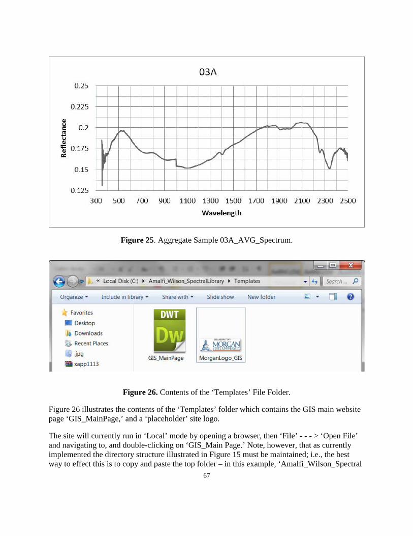
25. Aggregate Sample 03A_AVG_Spectrum 50
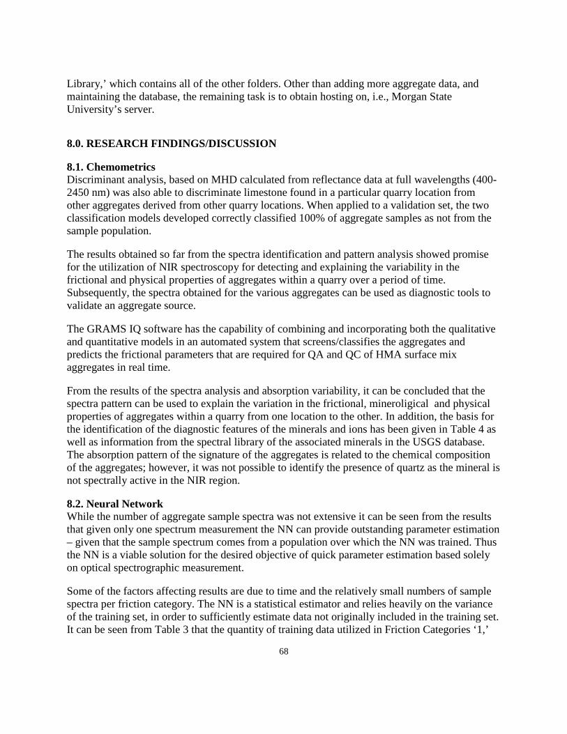
26. Contents of the ‘Templates’ File Folder 51
9
LIST OF TABLES
Tables: Page
1. Methods Used by US Transportation Agencies to Evaluate
Skid Resistance Properties 3
2. Comparison of Constitutive Models Which Simulate Deformation
Behavior of Granular Materials. 12
3. SHA Aggregate Sample Statistics 15
4. Spectra Pattern Attributable to Absorption Processes in Individual Minerals
Present in the Aggregate Samples Analyzed 22
5. Rock Type and Mineralogical Composition of Aggregates Produced from
Metagabbro Quartz-Diorite in 2012 and Metamorphic and Intrusive
Igneous Rocks in 2013 at Quarry 3 23
6. Rock Type and Mineralogical Composition of Aggregates Produced
from Gabbro at Quarry 6 25
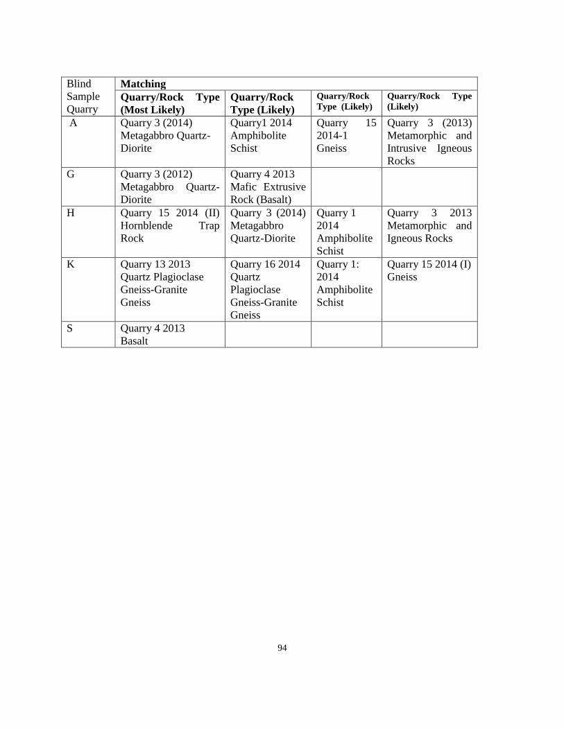
7. Summary of Blind Samples Matching 38
8. Test Results for the Full FC/SG/LA Estimator 43
9. Parameter Estimates Obtained for ‘Unknown’ Aggregate 26 43
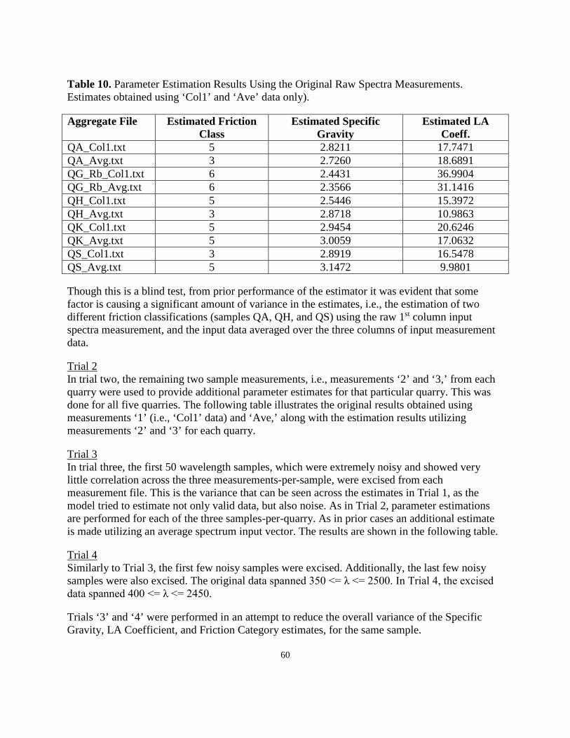
10. Parameter Estimation Results Using the Original Raw
Spectra Measurements 44
11. Compilation of Results of SHA Blind Tests 45
12. Parameter Estimation Results, Original Quarry 18A Data 46
10
11
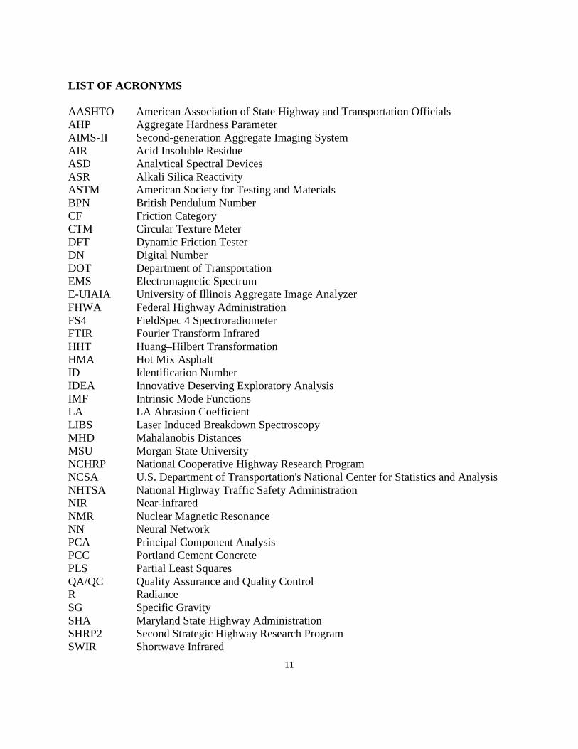
LIST OF ACRONYMS
AASHTO American Association of State Highway and Transportation Officials AHP Aggregate Hardness Parameter AIMS-II Second-generation Aggregate Imaging System AIR Acid Insoluble Residue ASD Analytical Spectral Devices ASR Alkali Silica Reactivity ASTM American Society for Testing and Materials BPN British Pendulum Number CF Friction Category CTM Circular Texture Meter DFT Dynamic Friction Tester DN Digital Number DOT Department of Transportation EMS Electromagnetic Spectrum E-UIAIA University of Illinois Aggregate Image Analyzer FHWA Federal Highway Administration FS4 FieldSpec 4 Spectroradiometer FTIR Fourier Transform Infrared HHT Huang–Hilbert Transformation HMA Hot Mix Asphalt ID Identification Number IDEA Innovative Deserving Exploratory Analysis IMF Intrinsic Mode Functions LA LA Abrasion Coefficient LIBS Laser Induced Breakdown Spectroscopy MHD Mahalanobis Distances MSU Morgan State University NCHRP National Cooperative Highway Research Program NCSA U.S. Department of Transportation's National Center for Statistics and Analysis NHTSA National Highway Traffic Safety Administration NIR Near-infrared NMR Nuclear Magnetic Resonance NN Neural Network PCA Principal Component Analysis PCC Portland Cement Concrete PLS Partial Least Squares QA/QC Quality Assurance and Quality Control R Radiance SG Specific Gravity SHA Maryland State Highway Administration SHRP2 Second Strategic Highway Research Program SWIR Shortwave Infrared
12
TRB Transportation Research Board USGS US Geological Survey USIGIS United States Imagery and Geospatial Information Services VIS Visible VNIR Visible-Near Infrared XRD X-ray Diffraction XRF X-ray Fluorescence
13
ACKNOWLEDGMENTS The authors wish to express their deepest appreciation and gratitude to the Maryland State Highway Administration (SHA) for its support throughout this project and for making it possible for Morgan State University (MSU) students to participate in a real-world transportation research; special thanks to Dr. Andrew Farkas and Ms. Anita Jones of MSU’s National Transportation Center (NTC) for supporting the students. The authors would also like to thank all the members of the technical team and staff, including Mr. Rodney Wynn, Mr. Dan Sajedi, Dr. Eric Frempong, Mr. Mark Wolcott, Mr. Barry Catterton, Mr. Eric Dougherty, Mr. Intikhab Haider, Mr. Darren Swift, Ms. Allison Hardt, Ms. Sharon Hawkins, Ms. Jacquae Rubin, and the others whose names I may have omitted for their assistance, advice, and expertise throughout the duration of this project.
14
EXECUTIVE SUMMARY A leading cause of death and injury in our Nation can be attributed to roadway crashes, with over 6 million reported annually between 1990 and 2000 (NHTSA, 2004). The frictional properties of road surfaces were listed as major factors in the cause of crashes, which in 2011 exceeded 32,000 fatalities in the United States. SHA is therefore tasked with the responsibility of ensuring that hot mix asphalt (HMA) used in road surface construction meets the stipulated requirements including frictional characteristics and skid resistance. However, the conventional methods being used by SHA in assessing and evaluating HMA surface mix are laborious, time-consuming, and expensive, hence the need for alternative methodologies that can be faster, more reliable, cost-effective, and nondestructive in nature. This research project included the development of methodologies that utilize spectral properties and characteristics of aggregate samples such as their wavelength and reflectance. The FieldSpec 4 spectroradiometer (FS4), developed by Analytical Spectral Devices (ASD), which is now known as PANalytical was utilized in this Project. The FS4 is recognized as one of the best portable high-resolution spectroradiometers for a wide range of scientific and engineering applications. Its 3 nanometer (nm) Visible-Near Infrared (VNIR) and 8 nm Shortwave Infrared (SWIR) spectral resolutions provide excellent spectral performance across the full range of the EMS (350 nm to 2500 nm). These superior spectral resolutions make it possible to detect and identify a wide variety of geospatial features and their elements/compounds. Due to the size of the aggregate samples (less than 2 centimeters in length), an ASD Turntable was also acquired in order to optimize the data acquisition process. The ASD Turntable, contains its own light source (4000 hour halogen light), and transforms the heterogeneity of the aggregate samples into a kind of homogeneous sample, thereby ensuring representative spectra for the samples that were extracted and collected more accurately and faster.
Two different methodologies were employed in this Project: 1 – Grams IQ Chemometrics Method and 2 – Neural Network (NN) Method. This multi-pronged approach, when proven, will undoubtedly offer the SHA options and flexibility in selecting the appropriate methodology for validating aggregate source and to some extent determining their properties. The spectra of 42 aggregate samples from 19 different quarries were extracted using the FS4, and the spectral data were analyzed using both Chemometrics and NN methodologies. The results obtained from both methodologies appear encouraging. The Chemometrics was able to discriminate limestone base on the quarry locations. It was also able to correctly determine (classified 100%) the source of aggregates samples in terms of not belonging to a given aggregate sample population. To a limited extent, this methodology was able to explain some of the aggregates’ frictional and physical variability within a given quarry over a period of time, thus making it a useful diagnostic tool. The NN, which relies heavily on the variance of the training set, was able to provide outstanding parameter estimations. Thus the NN is a viable solution for providing quick parameter estimations, based solely on the optical spectrographic measurement of the aggregate samples. It is hoped that these methodologies will enhance the SHA’s operational process by reducing the time and cost of evaluating HMA surface mix.
15
1.0. INTRODUCTION Roadway crashes are a leading cause of death and injury. Between 1990 and 2000, an average of 6.4 million highway crashes occurred annually nationwide (NHTSA 2004). In 2011, 32,310 people died in motor vehicle crashes, down 1.7 percent from 32,885 in 2010, according to the U.S. Department of Transportation's National Center for Statistics and Analysis of the National Highway Traffic Safety Administration (Liang 2013). The frictional properties of pavement surfaces and roadway condition play an important role in highway safety (Henry 2000). Pavement surfaces must maintain an adequate level of friction at the tire pavement interface in order to provide a safe surface for traveling vehicles (Liang 2013). The abrasion that occurs in asphalt concrete pavement over time from cars and trucks can polish the surface of the hot mix asphalt (HMA) and reduce friction, creating a serious safety concern, particularly under wet conditions. The Federal Highway Administration (FHWA) issued a Wet Skid Accident Reduction Program (Technical Advisory 5040.17) in 1980 in order to encourage state highway agencies to minimize wet weather skidding accidents by identifying and improving the sections of roadways with high occurrence of skid accidents and developing new surfaces at these sections to provide adequate and long-lasting skid resistance properties. The 1980 Technical Advisory was superseded in 2010 by a new advisory of Pavement Friction Management (FHWA 2010). It is therefore pertinent that the SHA ensures that flexible pavements that are being constructed or repaved using HMA have adequate skid resistance. Since the frictional characteristics of HMA are mainly influenced by the coarse aggregate exposed at the surface, the selection of the surface mix aggregates with adequate frictional and polishing characteristics and mineralogy of rock are crucial in providing the public with an acceptable level of friction on the roadway surface. To ensure that the surface mix aggregates that have adequate frictional and durability properties are utilized during construction, it is important to verify that the original source (quarry) of the aggregate has rock of excellent texture and the required mineralogy. Knowledge of the properties of minerals present in quarry rocks, as well as the preparation method can provide an excellent clue as to the suitability of the resulting aggregates. However, the quality assurance and quality control (QA/QC) procedures (Dynamic Friction Test, British Pendulum Test, and Acid Insoluble Residue Test) routinely used are time-consuming, expensive and not always reliable. With limited financial resources, there is a growing need for the development of rapid, cost-effective, nondestructive and accurate methods for assessing the quality of HMA surface mix aggregate’s original source. This research developed methodologies for using the portable spectroradiometer (ASD FieldSpec 4), a visible/infrared imaging spectrometer, for the validation of source approval of HMA surface mix aggregate and verified that the actual aggregate used during production matched the preapproved sources. Promising recent studies have shown that the portable FS4 can be used to determine the texture, mineralogy and composition of rocks as well as physical properties of aggregates (Schneider et al, 2009; Waiser et al, 2007; He and Song, 2006; Berg and Jarrard, 2002; Huntington et al 2010, and Sgavetti et al 2006).
16
17
2.0. LITERATURE REVIEW A review of existing literature which focused on current methodologies used for validating the original source of HMA surface mix aggregates was performed. Sources such as Science Direct, Google, Transportation Research Board (TRB), United States Imagery and Geospatial Information Services (USIGIS), and the State Department of Transportation (DOT) websites were queried. Over 100 documents were identified from this search and logged into the literature review database. The current state-of-the-practice was examined and documented, including but not limited to case studies of various states and other entities that have developed various methodologies for the validation process. Various validation methods and specifications were considered in order to assess the speed, accuracy, efficiency, versatility, safety and cost-effectiveness of these techniques. The information collected from the review was utilized to aid in the development of the spectroradiometric methodologies for the validation process. The various methodologies were divided into two categories: the conventional methods and fast, non-destructive methods. 2.1. Overview of Conventional Methods The frictional characteristics of HMA are influenced by the coarse aggregate exposed at the surface; therefore the selection of the surface mix aggregates with adequate frictional characteristics is crucial in providing the public with an acceptable level of friction on the roadway surface. Pavement surfaces must maintain an adequate level of friction at the tire pavement interface in order to provide a safe surface for traveling vehicles (Liang 2013). In ensuring that the surface mix aggregates that have adequate frictional and durability properties are utilized during construction, it is important to verify that the original source (quarry) of the aggregate has rock of adequate high friction texture and mineralogy. Knowledge of the mineral properties present in the aggregate as well as preparation methods of the aggregates, which can provide an excellent clue as to the suitability of the resulting aggregates, is very important. However, the QA/QC procedures routinely used are time-consuming, expensive and cumbersome. The conventional method usually includes the following tests on the aggregates:
● Los Angeles Abrasion Test (ASTM C535)
● British Pendulum Test (ASTM E303)
● Dynamic Friction Test (ASTM E 1911)
● Soundness Test (ASTM C88-90)
● Acid Insoluble Residue for Carbonate Aggregate (ASTM D3042)
● Petrography for Non-Carbonate Aggregate (ASTM C296-90)
According to Groeger et al. (2010), another survey of the specific methods being used by the states to control skid resistance was conducted by the Louisiana DOT in 2005/2006. The survey contains information from 27 states and Washington, DC. Table 1 contains a summary of the different methods used by these states in 2010.
18
Table 1: Methods used by US Transportation Agencies to Evaluate Skid Resistance Properties (Groeger et al, 2010)
Method Agencies
British Pendulum (BPN) New Jersey, Alabama Acid Insoluble Residual (AIR) Arkansas, Oklahoma, Wyoming, Washington, DC Sulfate Soundness Indiana Skid Trailer California, Florida, Georgia, Iowa, Mississippi, Montana,
Deval) Texas (BPN, AIR, LA Abrasion, Soundness, Skid Trailer) New York (AIR, Skid Trailer) Pennsylvania (Petrographic, BPN, AIR) Virginia (Geology, Skid Trailer, Local Experience) West Virginia (AIR, Skid Trailer)
Dynamic Friction Tester, BPN Maryland No Method-Restrictions Delaware (Use only Maryland approved quarries)
Kansas (Based on historical performance) Minnesota (No carbonate aggregate in wearing course)
In reviewing the conventional methods the advantages and limitations of each were taken into consideration. 2.2. British Pendulum Test This is the most common test and is specified in American Society for Testing and Materials (ASTM) E303. It is a portable apparatus that includes a pendulum with a spring-loaded rubber slider mounted at one end. The pendulum drops from a constant height, strikes a constant surface area with its rubber slider, and completes its swing to a degree proportional to the difference between its initial energy and the energy expended in sliding over the specimen surface. The decreased resulting energy of the pendulum is measured by an indicator needle which is mechanically activated by the pendulum as it passes through its point of lowest swing. The needle comes to rest at the point where the pendulum reaches its maximum forward swing, and the British pendulum number (BPN) is read off an arc-scale opposite the needle point. 2.2.1. Advantages It is one of the simplest and cheapest instruments used in the measurement of friction characteristics. It has the advantage of being easy to handle, both in the laboratory and in the field (Saito et al., 1996). 2.2.2. Limitations
19
Although it is widely suggested that the British Pendulum measurement is largely governed by the microtexture of the pavement surface, experience has shown that the macrotexture can also affect the measurements (Fwa et al., 2003; Lee et al., 2005). Additionally, Fwa et al., 2003; Liu et al., 2004) showed that the British Pendulum measurements could be affected by the macrotexture of pavement surfaces, aggregate gap width, or the number of gaps between aggregates; therefore this test has a high degree of variability. The test can also lead to misleading results on coarse-textured test surfaces (Lee et al., 2005). Other researchers pointed out that the BPN exhibited unreliable behavior when tested on coarse-textured surfaces (Forde et al., 1976; Salt, 1977; Purushothaman et al., 1988). Another problem with using the British Pendulum Tester is an extensive and ineffective calibration procedure. According to Groeger et al., 2010, the following are the other limitations of the procedures:
● The (BPN) after 9 hours of polishing is normally assumed to be the terminal polishing value for the aggregate.
● Polish number is affected by the aggregate selection technique. ● The additional time and polishing media can influence the outcome and might add more
uncertainties to the prediction. 2.3. Los Angeles Abrasion and Impact Test There are several methods to evaluate the potential of an aggregate to resist polishing made by traffic loading, and one test has been standardized under ASTM C535 and the American Association of State Highway and Transportation Officials (AASHTO) T 96. In the Los Angeles (LA) abrasion and impact test, the portion of aggregate retained on the #12 sieve is placed in a large rotating drum that has plates attached to its inner walls. A specified number of steel spheres are added to the drum, and it is rotated at 30 to 33 rotations per minute (rpm) for 500 revolutions. The material is then extracted and separated using the Sieve #12; the proportion of the materials remaining on the sieve is weighed. The difference between the new weight and the original weight is compared to the original weight and reported as LA value or percent loss. The LA abrasion and impact test is believed to assess an aggregate’s resistance to breakage rather than abrasion due to wear (Luce, 2006; Meninger, 2004). The advantage is that this test is fast and less cumbersome. 2.3.1. Limitations It is a common practice to assume that aggregates with lower LA abrasion loss and higher specific gravity (specific gravity, which can be converted to density) have better resistance to polishing. Many researchers believe that the LA abrasion test and other physical tests, like the freeze-thaw test, may not yield good predictions of field friction. Additionally, they believe that the reliability of predicting aggregate field polishing resistance, using a single laboratory test, is poor (West et al., 2001; Kowalski, 2007; Prasanna et al., 1999) 2.4. Dynamic Friction Tester The Dynamic Friction Testers (DFTs), as described by ASTM E 1911, consists of three rubber sliders and a motor that reaches 100 kilometer per hour (km/h) tangential speed. The rubber
20
sliders are attached to a 350 mm circular disk by spring-like supports that facilitate the bounce back of the rubber sliders from the pavement surface. The test is started while the rotating disk is suspended over the pavement and driven by a motor to a particular tangential speed. The disk is then lowered, and the motor is disengaged. Water is sprayed on the rubber and pavement interface through surrounding pipes to simulate wet weather friction. By measuring the traction force in each rubber slider using transducers and considering the vertical pressure that is reasonably close to the contact pressure of vehicles, the coefficient of friction of the surface is determined. The DFT can measure a continuous spectrum of dynamic frictional coefficients on pavement surfaces over the range of 0 to 80km/h with good reproducibility (Vollor and Hanson, 2006; Nippo, 2008). In addition, the DFT measurement at 20 km/h is an indication of the microtexture. 2.4.1. Advantages The advantage of DFT is that it provides a measure of surface friction as a function of sliding speed, either in the field or in a laboratory. It may be used to determine the relative effects of various polishing techniques on materials or material combinations. 2.4.2. Limitations The values measured in accordance with this method do not necessarily agree or directly correlate with those obtained from using other methods of determining friction properties or skid resistance (ASTM E 1911, 2009). As with most conventional methods, the turnaround time to obtain the results is long. 2.5. Acid Insoluble Test for Carbonate Aggregates. The aim of the acid insoluble test is to determine the amount and size distribution of non-carbonate (insoluble) material in carbonate aggregates (ASTM 3042, 2015). The test method covers determination of the percentage of insoluble residue in carbonate aggregates using hydrochloric acid solution to react the carbonates (ASTM 3042, 2015). The theory is based on the concept that the skid resistance of carbonate aggregates is related to the differential hardness of the minerals that constitute the aggregate. The softer minerals, in carbonate aggregate, usually wear away at a faster rate than the harder particles when subjected to polishing, and there is usually some attrition of the aggregate caused by the loss of softer particles. The advantage is that it is fast and less cumbersome. 2.5.1. Limitations The test tends to reflect the general trend of latter polishing values, but polishing values are not readily statistically predictable from these tests. 2.6. Petrographic Analysis Petrographic analysis of aggregates is normally performed in accordance with ASTM C296-90, & ASTM 295 in order to identify the mineral composition of aggregates and allow for the evaluation of predicted overall behavior. The general characteristics of the aggregate samples, including maximum particle size, textures and shape, are usually examined and recorded first. The main rock types are then identified and the relative proportions of the constituents will be
21
estimated using an optical (light) microscope. Color, grain size and degree of weathering are also recorded. 2.6.1. Advantages and Limitations It is a valuable tool in understanding the polishing process and to state recommendations for the use of aggregates. It also offers a good quantitative evaluation capability. The limitation is that this test requires an estimation of the relative proportions of the constituent minerals in the aggregate, thereby causing the result to vary from test to test. 2.7. Non Destructive Techniques for Aggregate Evaluation Unlike the traditional techniques/conventional methods used for aggregate evaluation, the non-destructive technique provides a fast, accurate and cost-effective method to eliminate the long turnaround time from sampling to testing usually associated with the conventional methods. The non-destructive technique measures the mineralogical properties of the aggregates. 2.7.1. Justification for the use of the Non-Destructive Technique There have been various studies in the past to correlate the skid resistance with mineralogical properties of aggregates. However, this section contains a comprehensive review of one of the studies performed by Kane et al., 2013. The objective of their work was to correlate the long-term skid resistance of a road surfacing aggregate, as measured in the laboratory, to the mineralogical properties of the aggregates. Three types of aggregates were studied: greywacke, granite and limestone used in asphalt surfacing. Petrographic analyses were carried out in an attempt to correlate aggregate mineralogy to aggregate polishing and consequently to friction and skid resistance. Optical microscopy was used to conduct the petrographic analysis of the aggregates. To determine the evolution of friction with polishing cycles of both aggregates and asphalt specimens, the Wehner-Schulze apparatus was used. Kane et al (2013) introduced a new parameter called the Aggregate Hardness Parameter (AHP), which measured on aggregate specimens after 188,000 polishing cycles and was related to aggregate frictional coefficients. The AHP is defined in Equation 1 as the sum of two aggregate hardness parameters: dmpM + cdM ……………. (1) where the first term ( dmpM) is the aggregate’s average Mohr’s Scale hardness value and the second term (cdM) is the contrast of hardness. Both values, which are usually obtained from the petrographic examination of the aggregates, are expressed as follows: dmpM =∑ dmi x pi ……………. (2) cdM = ∑ pi x dmi-dmb ……………. (3) Where dmi is the Mohs Scale of Hardness of each mineral found in the aggregate, pi is the percentage by mass of each mineral found in the aggregate and dmb is the Mohs scale of hardness of the most abundant mineral found in the aggregate Initial results indicated that aggregate hardness parameter is a good indicator of the frictional resistance of an aggregate. In addition to monitoring the evolution of the friction coefficient, profile measurements on aggregate mosaics were carried out using a confocal microscope in
22
order to assess the evolution of texture (Kane et al (2013)). Microtexture measurements confirmed different levels of polishing for the different types of aggregates. Their findings confirmed that the skid resistance of road surfaces after a long period of use is driven by the characteristics of the aggregates in the asphalt. Kane et al (2013) discovered that the aggregate hardness parameter indicated the ability of an aggregate to retain its microtexture and its friction properties. From the prior literature search it is pertinent to share that any non-invasive technique that can determine the mineralogy of aggregate can be used to effectively determine the frictional characteristics of the aggregates. For this project, a literature search of the past techniques used to measure the mineralogy and microstructure of aggregates, both qualitatively and quantitatively, was completed. 2.7.2. Laser Induced Breakdown Spectroscopy (LIBS) In 2012, the Transportation Research Board, through the Innovations Deserving Exploratory Analysis (IDEA) Program, investigated the feasibility of using a laser monitoring system to provide real-time data to characterize aggregate properties in a laboratory or field environment. The study made use of the known physical, chemical and mechanical properties and aggregate criteria as defined by AASHTO and ASTM, and correlated these properties with spectral emission data through Laser Induced Breakdown Spectroscopy (LIBS). LIBS technology was used to employ an automatic laser monitoring system in order to provide real-time data of aggregate quality in a field environment (Chesner and McMillan, 2012). In the study, a multivariate statistical modeling technique was used to provide information on the latent properties of the aggregate material in order to discriminate between aggregate types and identify specific aggregate properties (Chesner and McMillan, 2012). Three state DOTs -- New York (NYSDOT), Kansas (KSDOT), and Texas (TXDOT) -- participated in the research effort to demonstrate the subject technology LIBS. Each DOT supplied specific aggregate for laser calibration testing to determine if the technology could be used to identify whether specific aggregates were good or poor, as defined by the respective state’s specification criteria. Aggregates from New York were studied to see if the Acid Insoluble Residue (AIR) content of carbonate aggregates could be modeled and whether a compositional blend of noncarbonated rocks, which are almost entirely composed of quartz or silicate minerals, mixed with limestone could be quantified. Aggregates from Kansas were examined to determine whether the original (source) bed in a quarry, from which an unknown aggregate sample was extracted, could be identified by modeling the characteristics of the aggregate from each bed. D-cracking susceptible aggregates from Kansas were also analyzed to determine if modules could be developed to differentiate between aggregates that passed and failed KSDOT D-Cracking test criteria. Aggregates from Texas were examined to determine if a compositional blend of chert and quartz could be quantified (i.e., the percent chert in the blend, whether high and low reactive cherts could be classified and whether four cherts with different degrees of alkali silica reactivity (ASR) could be differentiated.) The results of the research suggested that multivariate discriminate modeling of laser induced spectra can be used to correlate spectral output data with aggregate types and aggregate
23
properties (Chesner and McMillan 2012). This was not surprising, since it is reasonable to assume that the engineering properties of aggregates as defined by AASHTO and ASTM test criteria are dependent in part on the chemical and mineralogical composition of the aggregate material (Chesner and McMillan, 2012). While such an assumption is reasonable it is worth noting that up until now few studies have effectively developed correlations between the chemical and mineralogical properties of aggregates, and most engineering properties. 2.7.2.1. Advantages The LIBS provides a real time technique for evaluating the frictional characteristics of aggregates. According to Chesner and McMillan (2012), the turnaround times from sampling to the completion of testing vary widely depending on the test method but can range from a few hours to a few days to several weeks and even several months. Consequently, they observed that aggregate quality assurance is in great part dependent on the collection, testing, and preapproval of aggregate sources prior to the actual material production process. Subsequently, Chesner and McMillan (2012) observed that many agency quality assurance plans require that additional samples be collected during the production process to verify that the actual aggregate employed during production matches the preapproved sources. Unfortunately according to their observation, when such methods are employed, the pavement or concrete structure is typically in place by the time test results became available. In certain instances, failure of such verification to comply with the appropriate specification necessitates the removal and replacement of the newly installed structure. Subsequently, eliminating the long turnaround times from sampling to the completion of tests associated with the conventional method is the major advantage of the LIBS procedure. The procedure is also cost-effective and simple. 2.7.2.2 Limitations: It is pertinent to note that LIBS technology adopted in the NCHRP IDEA Project 150 uses a laser-scanning system which is a type of active remote sensing procedure that ablates (removes) sections of the surface material/samples through vaporization. The results obtained through this method can vary depending on several factors including the power of the laser and resulting plasma. 2.8. FieldSpec 4 Spectroradiometer The FieldSpec 4 Spectroradiometer (FS4) uses the principles of Visible and Near-infrared (NIR) reflectance spectrometry to determine the mineralogy and physical properties of aggregate. This technology provides an efficient and cost-effective alternative to the traditional lab-based analysis. With NIR reflectance analysis, rapid non-destructive measurements can be taken in the field or in a controlled laboratory environment (Kastanek and Greenwood, 2013). The instrument covers the visible (VIS) and the NIR regions of the electromagnetic spectrum (EMS). When the NIR energy interacts with the sample, part of the electromagnetic light ray can be absorbed, reflected, or transmitted through the sample (ASD Inc., 2012). Figure 1 shows all the possible interactions of NIR with solids or target material (ASD Inc., 2012). The NIR spectra are further differentiated by the sample accessory used for spectra collection. Quantitative and qualitative calibration models can be developed from the spectra collected for rapid characterization of aggregates mineralogy and physical properties by using chemometrics software. GRAMS IQ, a
24
multivariate chemometrics software from Thermo Fisher Scientific, Woodbridge, NJ, is usually used to create the quantitative and qualitative multivariate statistical models from the spectra derived from the FS4. Recent studies have shown that the portable FS4 can be used to determine the texture, mineralogy and composition of rocks as well as physical properties of aggregates (Schneider et al, 2009; Waiser et al, 2006; He and Song, 2006; Berg and Jarrard, 2002; Huntington et al 2010). 2.8.1. Advantages It is an alternative method that eliminates the long turnaround time associated with the traditional methods without reduction of accuracy. According to Quattlebaum and Nusbaum, 2001, this nondestructive analytical technique takes advantage of characteristic absorption and scattering of photons resulting from OH- and H20 vibrational processes to accurately diagnose the mineralogy and composition of geological materials. Unlike LIBS, the FS4 employs passive remote sensing procedures, which utilize selected sections of EMS between 350-2500 nm (the VIS, NIR). This technique does not tamper with the sample surface. 2.8.2. Limitation In order to derive maximum benefit from the use of the equipment, the qualitative and quantitative multivariate statistical models must be effectively developed with the appropriate software. According to Zofka et al., 2013, spectrosocopic evaluation of aggregates will always be a challenging task, especially when dealing with aggregates from different compositional blends. In such cases more work is needed to develop robust and universal procedures.
25
Figure 1: Near-Infrared Interactions with Target Material (ASD Inc., 2012)
2.9. Other Non-Destructive Methods Apart from the NCHRP IDEA Project 150, more work on using non-destructive testing for evaluation of aggregates properties was also conducted. Post and Crawford (2014) used the near infrared spectral for the identification of clay minerals. Satpathy et al., 2010 used hyperspectral remote sensing to provide physics-chemistry (mineralogy, chemistry, morphology) of the earth’s surface. Their methodology is useful for mapping potential host rocks, alteration assemblages and mineral characteristics. Some pure pixel end member for the target mineral and the backgrounds were used to account for the spectral angle mapping and matched filtering with the results were validated with respect of field study. Zofka et al. (2013) under the Second Strategic Highway Research Program (SHRP2) evaluated the use of portable spectroscopy devices and their capability to fingerprint typical construction materials. Fingerprinting of typical materials requires developing acceptable spectra of specified chemical compositions with laboratory-based equipment and then comparing the material being fingerprinted against those spectra (Zofka et al., 2013). On the basis of the above requirements they developed a library of reference spectra for common materials used in highway construction. They further developed relatively simple and easy-to-use non-destructive testing procedures and protocols that inspectors could use in the field to ensure quality construction. The Spectroscopic techniques evaluated in the laboratory included Fourier Transform Infrared (FTIR) spectroscopy, Size-exclusion Chromatography, Nuclear Magnetic Resonance (NMR), X-ray Fluorescence (XRF), and X-ray Diffraction (XRD). The materials used included epoxy coatings, adhesives, traffic paints, Portland cement concrete (PCC) with chemical admixtures and curing compounds, asphalt binders, emulsions, and mixes with polymer additives. Through a comprehensive literature review, in combination with experience as well as survey and workshops results, they evaluated the most promising combinations of techniques and materials. The laboratory testing phase of the study indicated that three methods were most promising for field applications: FTIR, XRF and Raman. It was finally discovered that a compact FTIR spectrometer working in the Portland cement concrete (PCC) mode was the most successful device to fingerprint pure chemical compounds (i.e., epoxides, waterborne paints, polymers, and chemical additives) and to detect additives or contaminants in complex mixtures (i.e, PCC, asphalt binders, emulsion and mixes). Pavement friction, one of the main factors contributing to road safety, depends mainly on surface texture. However, despite its importance being corroborated by the numerous investigations attempting to predict it, the manner in which texture is related to friction remains widely unknown. Rado and Kane, 2014, explored the friction-texture relationship based on a new signal processing method called Huang–Hilbert Transformation, or HHT. This method allows empirical decomposition of a texture profile to a set of basic profiles in a limited number, called Intrinsic Mode Functions, or IMFs. Each IMF contains a given interval of amplitudes and frequencies. From the obtained IMFs, a set of four new functions called Base Intrinsic Mode Functions, or BIMF, was computed based on the frequency and power content of the underlying IMFs and was characterized using the Hilbert Transformation technique to obtain the scale-dependent norm
26
frequency and amplitude profiles. Furthermore, these two parameters were correlated with the pavement friction from a multiple regression analysis. This analysis was applied to a set of texture and friction data measured through test track surfaces in France and lab samples of concrete in the United States. The textures and friction values were measured with the Circular Texture Meter (CTM) and the DFT, respectively. The results showed a good correlation between the BIMF's parameters to friction, thus opening a promising new means for characterizing texture in relation to friction. Moaveni et al., (2014), used aggregates imaging systems to develop regression-based statistical models for determining aggregate polishing and degradation trends by considering both rate and magnitude of changes in shape properties. Since aggregate gradation and shape properties are known to affect pavement mechanistic response and performance significantly, under repeated traffic loading, aggregate particles in pavement courses are routinely subjected to degradation through attrition, impact, grinding and polishing mechanism. In their investigation Moaveni et al (2014) used two advanced and validated aggregate imaging systems – an enhanced University of Illinois aggregate image analyzer (E-UIAIA) and a second-generation aggregate imaging system (AIMS-II) – for capturing changes in shape and size properties of aggregate particles caused by breakage, abrasion, and polishing actions. They used the micro-Deval apparatus in the laboratory to evaluate field degradation and polishing resistance of 11 aggregate materials with different mineralogical properties, collected throughout Illinois and neighboring states. In their investigation, more than 26,000 particles were scanned with both imaging systems at various time intervals, and changes in aggregate morphological indexes were recorded. Despite differences in image acquisition and processing capabilities, both E-UIAIA and AIMS-II successfully quantified changes in morphological properties of particles from micro-Deval tests. However, AIMS-II more closely reflected historical data on aggregates’ frictional properties obtained by the Illinois Department of Transportation.
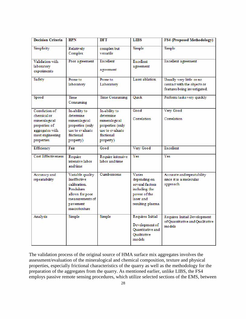
3.0. COMPARISON OF CURRENT AND PROPOSED METHODOLOGIES A comparison of current methodologies and the proposed spectroradiometric (FS4) methodology was conducted in order to assess the speed, accuracy, efficiency, versatility, safety, repeatability, and cost-effectiveness of each technique. These evaluating criteria are similar to those Wimssat et al. (2009) adopted in evaluating their developed high-speed nondestructive testing procedures for design evaluation and construction inspection. Three of the most promising methodologies currently used in evaluating the frictional characteristics of aggregates – BPN, DFT and LIBS – were compared with the proposed FS4 technique. The information collected from the review was utilized to aid in the development of the spectroradiometric methodologies for the validation process of the aggregate source. Table 2 shows the results of the comparison analysis developed in this study. From the literature study conducted and the results of the comparison analysis in Table 2, it was also shown that FS4 provides an efficient cost-effective alternative to traditional lab-based analysis of the frictional properties of aggregate. As mentioned earlier, with NIR reflectance analysis, rapid non-destructive measurements can be taken in the field or in a controlled laboratory environment. Quantitative calibration models can be developed for rapid
27
characterization of aggregate frictional attributes and properties. In addressing the limitation of this technique, Kastanek and Greenwood, 2013 suggested that coupling this technology with hyperspectral imagery and improved spatial statistical methodologies breaks the bottleneck of sample collection and lab analysis and facilitates real-time aggregates characteristics assessment. Subsequently, the project shall entail the development of methodologies for using the portable FS4, for the validation of source approval of HMA surface mix aggregate as well as to verify that the actual aggregate used during production matches the preapproved sources. The FS4 will facilitate real time evaluation of the frictional characteristics of aggregates used in the production of HMA, without the conventional sample preparation and laboratory testing.
Table 2: Comparison of Constitutive Models Which Simulate Deformation Behavior of Granular Materials.
28
The validation process of the original source of HMA surface mix aggregates involves the assessment/evaluation of the mineralogical and chemical composition, texture and physical properties, especially frictional characteristics of the quarry as well as the methodology for the preparation of the aggregates from the quarry. As mentioned earlier, unlike LIBS, the FS4 employs passive remote sensing procedures, which utilize selected sections of the EMS, between
29
350 – 2500 nm (VIS - NIR). The reflected or emitted electromagnetic radiation from the sample (aggregate material) surfaces will be measured. This technique does not tamper with the sample surface. The spectra collected from the aggregates will be standardized to enable the spectrum of unknown materials to be compared to known material after calibration/correction consistently. The high-resolution FS4 has been designed for faster, more precise spectral data collection. It is portable, possesses enhanced spectral resolution of 8 nm, and ruggedized for challenging field terrain. Its extended wireless range provides more flexibility in conducting field work easily. The FS4, with an 8 nm resolution will make it ideal for building spectral libraries especially when required to support critical missions/tasks, site validation, and groundtruthing.
4.0. METHODOLOGIES
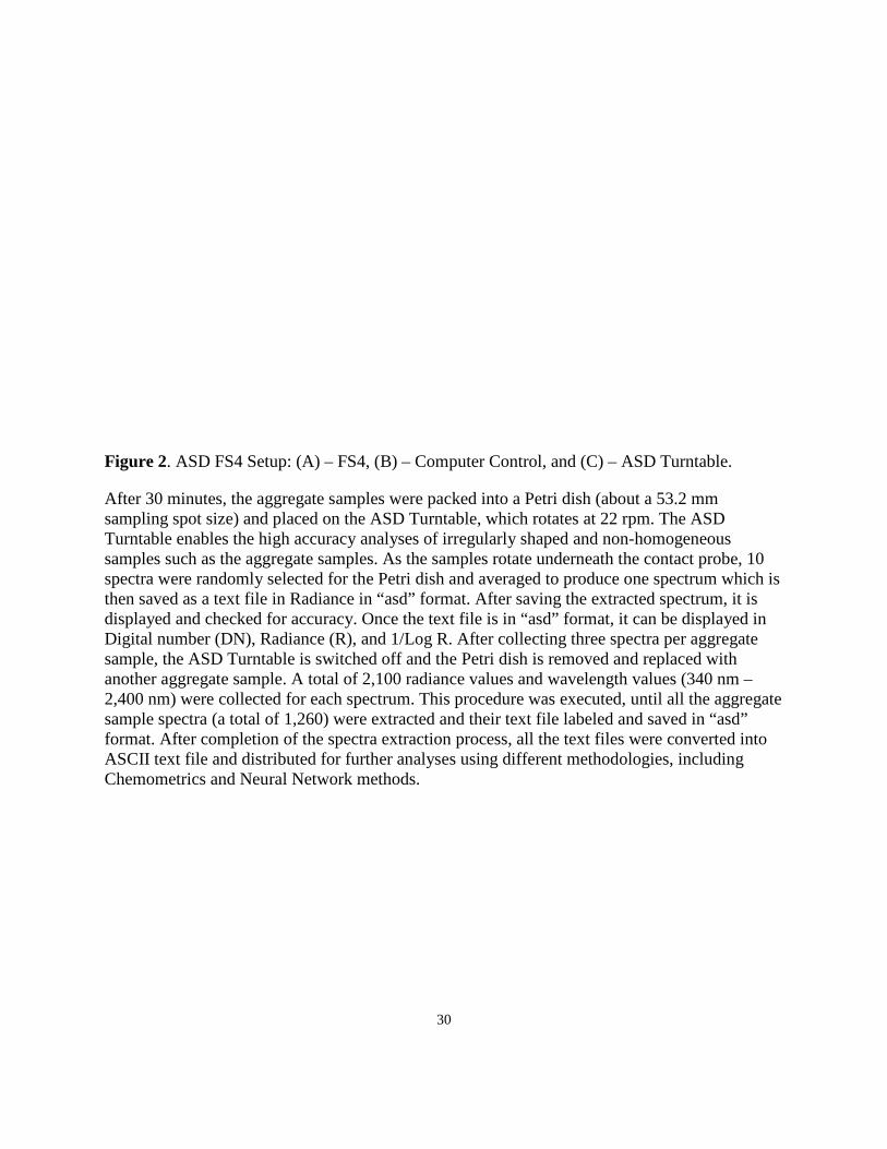
4.1. Introduction Initially, three different methodologies were considered for this Project: 1 – Statistical Analysis System (SAS), 2 –Grams IQ Chemometrics, and 3 –Neural Network (NN). This multi-pronged approach was used in order to provide the SHA with flexible options in determining the most efficient and cost-effective methodology in validating the HMA surface mix aggregate. SAS, a suite of software originally developed at North Carolina State University, was supposed to be used to perform multivariate discriminate modeling of the spectra extracted from the aggregate samples. However, because of its stringent requirements, including the need for large and continuous datasets which were not available at that time, it was decided not to continue with it at this time. Future efforts will be geared toward the collection of more aggregate data samples which would then enable the use of SAS. Details of the other two methods (chemometrics and NN) are provided in subsequent sections below. 4.2. Data – The Aggregate Samples A total of 42 aggregate samples from 19 different quarries were provided by the SHA to Morgan State University (MSU) for analyses using the FS4. The samples were carefully kept in the lab, in glass jars, under normal temperature and dry conditions. In order to maintain confidentiality of the quarries, identification numbers (IDs) were assigned to each of the samples (Appendix A). Great care was taken during the handling of each sample during the extraction of their spectra; all samples were returned to their respective jars after the spectra extractions were completed. 4.3. Aggregate Spectra Extraction The aggregate samples were logged and identification numbers (IDs) were assigned to each sample jar. The jars were sorted and placed in ascending order on a clean table in the lab. The FieldSpec 4 and its Turntable were assembled on an adjacent table and turned on for 30 minutes in order to attain the optimum operational temperature based on the stipulated instructions from the manufacturer (ASD, Inc.) (Figure 2).
After 30 minutes, the aggregate samples were packed into a Petri dish (about a 53.2 mm sampling spot size) and placed on the ASD Turntable, which rotates at 22 rpm. The ASD Turntable enables the high accuracy analyses of irregularly shaped and non-homogeneous samples such as the aggregate samples. As the samples rotate underneath the contact probe, 10 spectra were randomly selected for the Petri dish and averaged to produce one spectrum which is then saved as a text file in Radiance in “asd” format. After saving the extracted spectrum, it is displayed and checked for accuracy. Once the text file is in “asd” format, it can be displayed in Digital number (DN), Radiance (R), and 1/Log R. After collecting three spectra per aggregate sample, the ASD Turntable is switched off and the Petri dish is removed and replaced with another aggregate sample. A total of 2,100 radiance values and wavelength values (340 nm – 2,400 nm) were collected for each spectrum. This procedure was executed, until all the aggregate sample spectra (a total of 1,260) were extracted and their text file labeled and saved in “asd” format. After completion of the spectra extraction process, all the text files were converted into ASCII text file and distributed for further analyses using different methodologies, including Chemometrics and Neural Network methods.
Note(s): 1 – In the ‘Number of Samples’, the left-most number is the total number of samples in that ‘Friction Category.’ In the right-side split cell, the upper number is the number of samples that have all three parameters – SG, LA, and BPN. The lower number is the number of samples that have only SG and LA. The aggregate information given above is utilized by both the Chemometrics and Neural-Network methodologies. These two methodologies are described in more detail in the following sections. 5.0. CHEMOMETRICS METHOD 5.1. Introduction This chapter contains data analysis of the spectra of 42 aggregate samples collected using the FieldSpec 4 Spectrometer. The analysis was conducted using the GRAMS IQ chemometrics software from Thermo Fisher Scientific, Woodbridge, NJ. The GRAMS Spectroscopy Software Suite is the premier solution for visualizing, processing and managing spectroscopy data offering broad compatibility with many different instrument data types and a simple user interface. The GRAMS software combines spectral data and reference data to predict class membership (qualitative model). Detailed results from two quarries (Quarries 17 and 18) are presented in this Report. Results of the spectral analysis and blind test matching are also presented in this chapter.
32
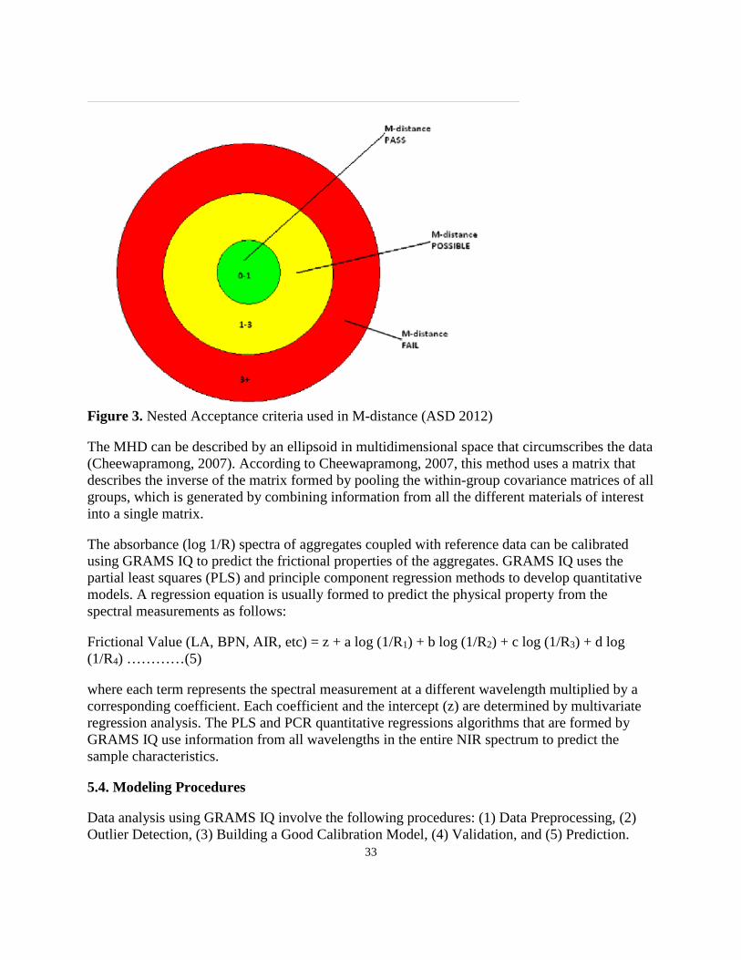
5.2. Research and Modeling Objectives A spectra library for each of the quarries was developed in order to be able to validate the source of the HMA surface aggregate and conduct classification models. The GRAMS IQ software, classification models compare the spectrum of an unknown aggregate sample to that of a group of known spectra. Through this process the model would be able to determine whether the unknown aggregate sample resembles any of the known aggregate samples. This classification model is especially useful for the validation of source approval of HMA surface aggregates. 5.3. Brief Review of Multivariate Statistical Modeling GRAMS IQ software combines spectra data and reference data to develop qualitative (classification) and quantitative (concentration) models through the use of regression methods with statistics. In order to develop a qualitative (classification) model, GRAMS IQ uses discriminant analysis which is based on the Principal Component Analysis (PCA) compression of the spectral data into scores. PCA is a reduction technique that extracts from a large number of variables to a much smaller number of new variables, which account for most of the variability between samples and contain information from the entire spectrum (Cheewapramong, 2007). Thus, the PCA decomposes the training set spectra into mathematical spectra like loading vectors, factors, and principal components that represent the most common variations to all the data. The principal components scores, from spectra of samples in a training set, are then used to calculate the Mahalanobis matrices, which are derived from the Mahalanobis Distances (MHD), and discriminant models are then constructed. The Mahalanobis Distance (MHD), is the mathematical quantity that defines the position, size and shape of the ellipsoid for all clusters and is defined by a multidimensional distance D defined by the matrix equation as follows: D2= (x-x' )M(x-x ' )……………. (4) Where D is the MHD, x is a vector consisting of optical readings at several wavelengths which describes the position in multidimensional space corresponding to the spectrum of a given sample, xi is the vector describing the position of a reference point in space, and M is the pooled inverse covariance matrix describing distance measures in the multidimensional space of interest (Mark and Tunnel (1985)). Samples with MHD less than 3 σ (three standard deviations) are considered to be members of the same group of spectra used to develop the model while spectra with MHD greater than 3 σ are considered to be Non-members (Figure 3). MHD from a statistical viewpoint takes the sample variability into account.
33
Figure 3. Nested Acceptance criteria used in M-distance (ASD 2012) The MHD can be described by an ellipsoid in multidimensional space that circumscribes the data (Cheewapramong, 2007). According to Cheewapramong, 2007, this method uses a matrix that describes the inverse of the matrix formed by pooling the within-group covariance matrices of all groups, which is generated by combining information from all the different materials of interest into a single matrix. The absorbance (log 1/R) spectra of aggregates coupled with reference data can be calibrated using GRAMS IQ to predict the frictional properties of the aggregates. GRAMS IQ uses the partial least squares (PLS) and principle component regression methods to develop quantitative models. A regression equation is usually formed to predict the physical property from the spectral measurements as follows: Frictional Value (LA, BPN, AIR, etc) = z + a log (1/R1) + b log (1/R2) + c log (1/R3) + d log (1/R4) …………(5) where each term represents the spectral measurement at a different wavelength multiplied by a corresponding coefficient. Each coefficient and the intercept (z) are determined by multivariate regression analysis. The PLS and PCR quantitative regressions algorithms that are formed by GRAMS IQ use information from all wavelengths in the entire NIR spectrum to predict the sample characteristics. 5.4. Modeling Procedures Data analysis using GRAMS IQ involve the following procedures: (1) Data Preprocessing, (2) Outlier Detection, (3) Building a Good Calibration Model, (4) Validation, and (5) Prediction.
34
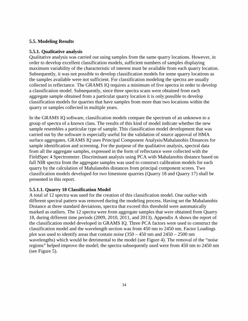
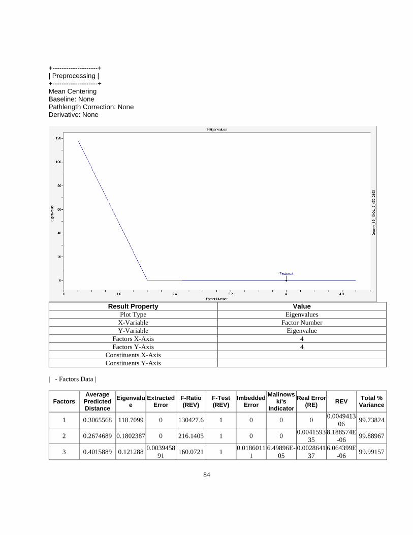
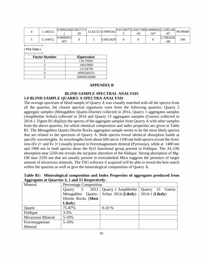
5.5. Modeling Results 5.5.1. Qualitative analysis Qualitative analysis was carried out using samples from the same quarry locations. However, in order to develop excellent classification models, sufficient numbers of samples displaying maximum variability of the characteristic of interest must be available from each quarry location. Subsequently, it was not possible to develop classification models for some quarry locations as the samples available were not sufficient. For classification modeling the spectra are usually collected in reflectance. The GRAMS IQ requires a minimum of five spectra in order to develop a classification model. Subsequently, since three spectra scans were obtained from each aggregate sample obtained from a particular quarry location it is only possible to develop classification models for quarries that have samples from more than two locations within the quarry or samples collected in multiple years. In the GRAMS IQ software, classification models compare the spectrum of an unknown to a group of spectra of a known class. The results of this kind of model indicate whether the new sample resembles a particular type of sample. This classification model development that was carried out by the software is especially useful for the validation of source approval of HMA surface aggregates. GRAMS IQ uses Principal Component Analysis/Mahalanobis Distances for sample identification and screening. For the purpose of the qualitative analysis, spectral data from all the aggregate samples, expressed in the form of reflectance were collected with the FieldSpec 4 Spectrometer. Discriminant analysis using PCA with Mahalanobis distance based on full NIR spectra from the aggregate samples was used to construct calibration models for each quarry by the calculation of Mahalanobis distances from principal component scores. Two classification models developed for two limestone quarries (Quarry 18 and Quarry 17) shall be presented in this report. 5.5.1.1. Quarry 18 Classification Model A total of 12 spectra was used for the creation of this classification model. One outlier with different spectral pattern was removed during the modeling process. Having set the Mahalanobis Distance at three standard deviations, spectra that exceed this threshold were automatically marked as outliers. The 12 spectra were from aggregate samples that were obtained from Quarry 18, during different time periods (2009, 2010, 2011, and 2013). Appendix A shows the report of the classification model developed in GRAMS IQ. Three PCA factors were used to construct the classification model and the wavelength section was from 450 nm to 2450 nm. Factor Loadings plot was used to identify areas that contain noise (350 – 450 nm and 2450 – 2500 nm wavelengths) which would be detrimental to the model (see Figure 4). The removal of the “noise regions” helped improve the model; the spectra subsequently used were from 450 nm to 2450 nm (see Figure 5).
35
Figure 4. Factor Loading Plot Showing Scratchy/Rough Regions of 350-450 nm & 2450-2500 nm Due to Noise.
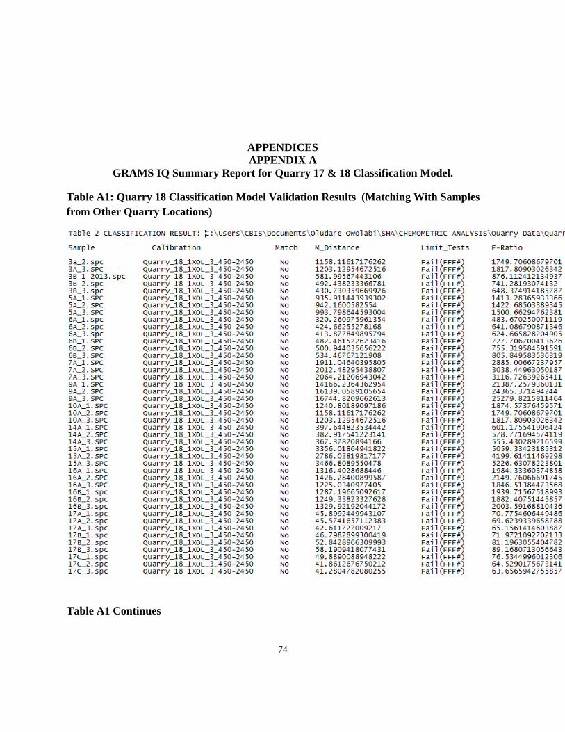
The model results indicated a 100% classification accuracy for the aggregates from Quarry 18. Correct classification refers to the percentage of spectra samples from other quarry locations outside Quarry 18 in a validation set, non-matched with spectra in a calibration set (Cheewapramong, 2007). This result suggested that the classification model was able to reveal any aggregates that were not derived from Quarry 18 (see Table A1 (Appendix A) –a sample section of the classification results obtained for Quarry 18).
36
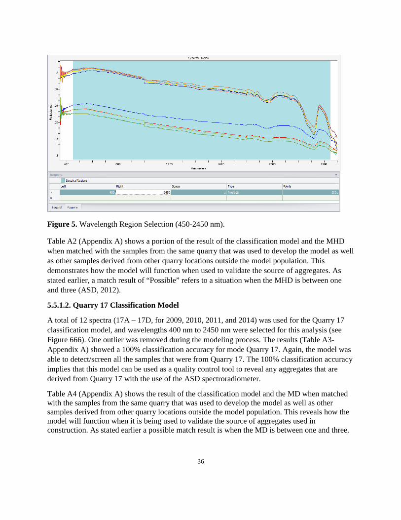
Figure 5. Wavelength Region Selection (450-2450 nm).
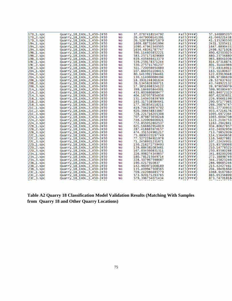
Table A2 (Appendix A) shows a portion of the result of the classification model and the MHD when matched with the samples from the same quarry that was used to develop the model as well as other samples derived from other quarry locations outside the model population. This demonstrates how the model will function when used to validate the source of aggregates. As stated earlier, a match result of “Possible” refers to a situation when the MHD is between one and three (ASD, 2012).
5.5.1.2. Quarry 17 Classification Model
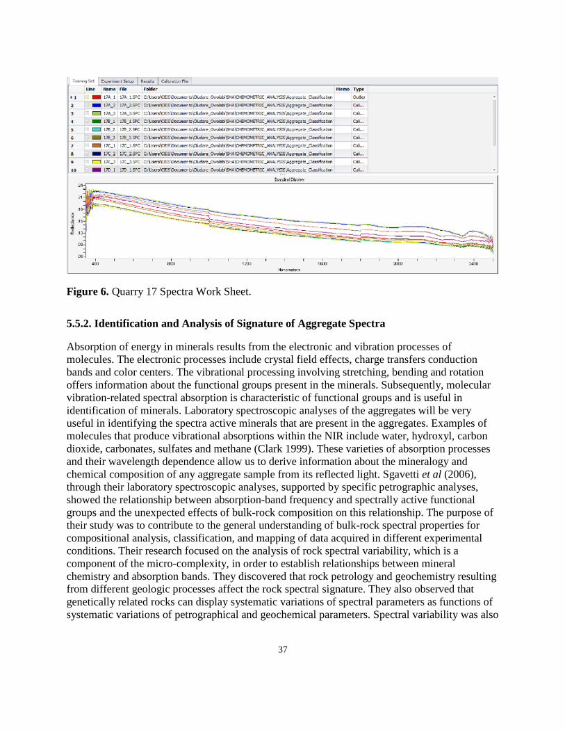
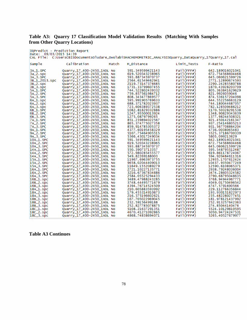
A total of 12 spectra (17A – 17D, for 2009, 2010, 2011, and 2014) was used for the Quarry 17 classification model, and wavelengths 400 nm to 2450 nm were selected for this analysis (see Figure 666). One outlier was removed during the modeling process. The results (Table A3-Appendix A) showed a 100% classification accuracy for mode Quarry 17. Again, the model was able to detect/screen all the samples that were from Quarry 17. The 100% classification accuracy implies that this model can be used as a quality control tool to reveal any aggregates that are derived from Quarry 17 with the use of the ASD spectroradiometer.
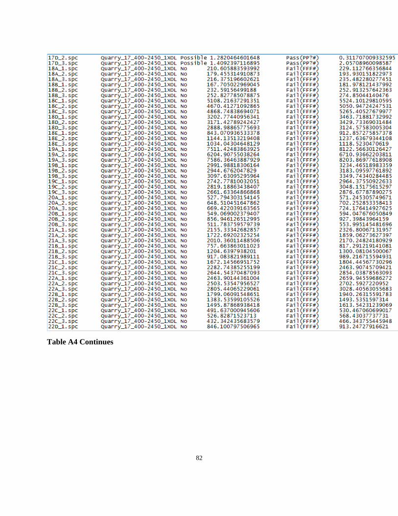
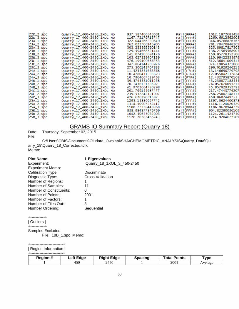
Table A4 (Appendix A) shows the result of the classification model and the MD when matched with the samples from the same quarry that was used to develop the model as well as other samples derived from other quarry locations outside the model population. This reveals how the model will function when it is being used to validate the source of aggregates used in construction. As stated earlier a possible match result is when the MD is between one and three.
37
Figure 6. Quarry 17 Spectra Work Sheet.
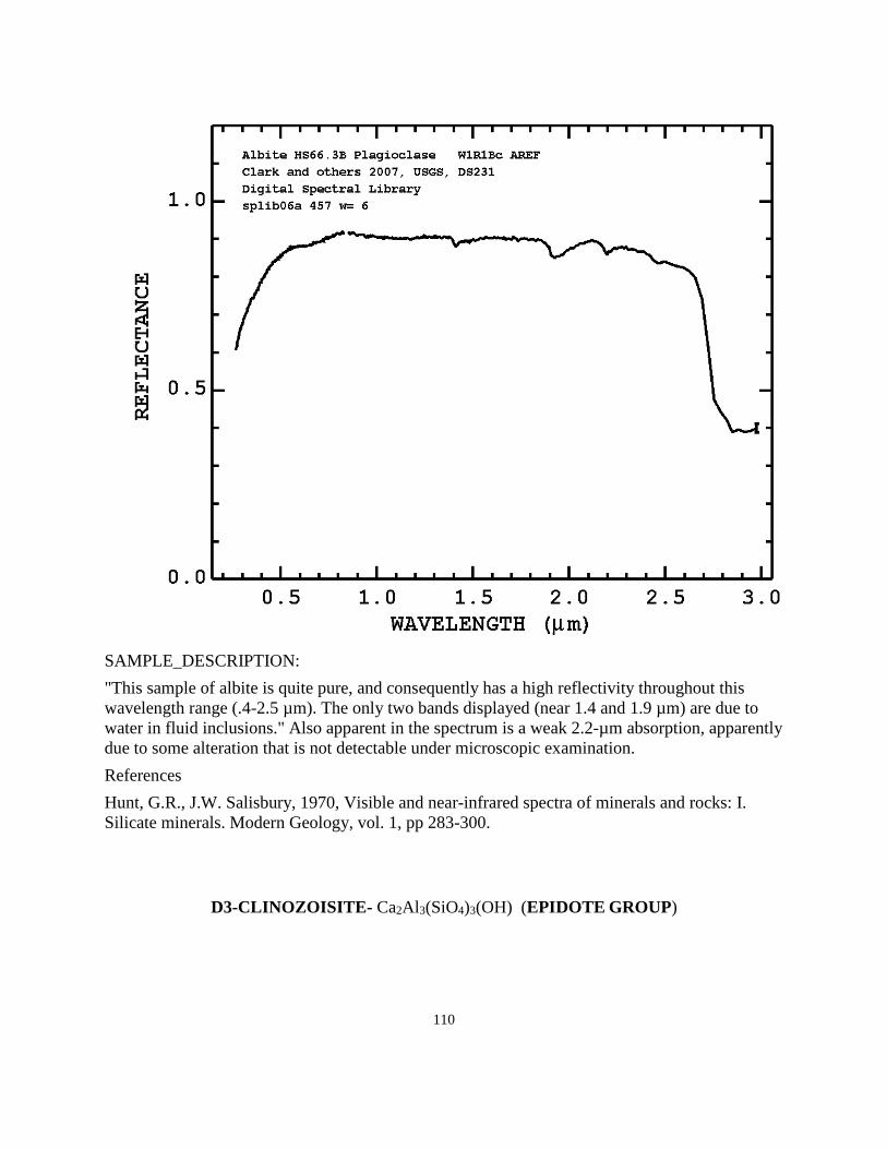
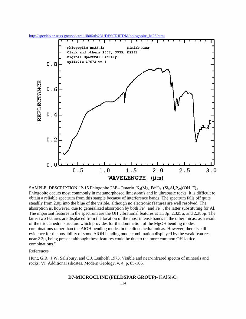
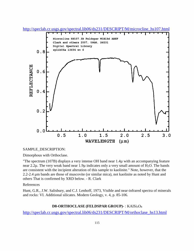
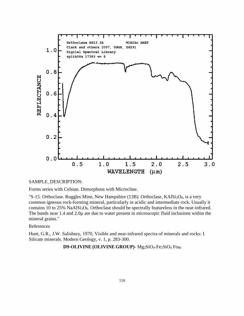
5.5.2. Identification and Analysis of Signature of Aggregate Spectra Absorption of energy in minerals results from the electronic and vibration processes of molecules. The electronic processes include crystal field effects, charge transfers conduction bands and color centers. The vibrational processing involving stretching, bending and rotation offers information about the functional groups present in the minerals. Subsequently, molecular vibration-related spectral absorption is characteristic of functional groups and is useful in identification of minerals. Laboratory spectroscopic analyses of the aggregates will be very useful in identifying the spectra active minerals that are present in the aggregates. Examples of molecules that produce vibrational absorptions within the NIR include water, hydroxyl, carbon dioxide, carbonates, sulfates and methane (Clark 1999). These varieties of absorption processes and their wavelength dependence allow us to derive information about the mineralogy and chemical composition of any aggregate sample from its reflected light. Sgavetti et al (2006), through their laboratory spectroscopic analyses, supported by specific petrographic analyses, showed the relationship between absorption-band frequency and spectrally active functional groups and the unexpected effects of bulk-rock composition on this relationship. The purpose of their study was to contribute to the general understanding of bulk-rock spectral properties for compositional analysis, classification, and mapping of data acquired in different experimental conditions. Their research focused on the analysis of rock spectral variability, which is a component of the micro-complexity, in order to establish relationships between mineral chemistry and absorption bands. They discovered that rock petrology and geochemistry resulting from different geologic processes affect the rock spectral signature. They also observed that genetically related rocks can display systematic variations of spectral parameters as functions of systematic variations of petrographical and geochemical parameters. Spectral variability was also
38
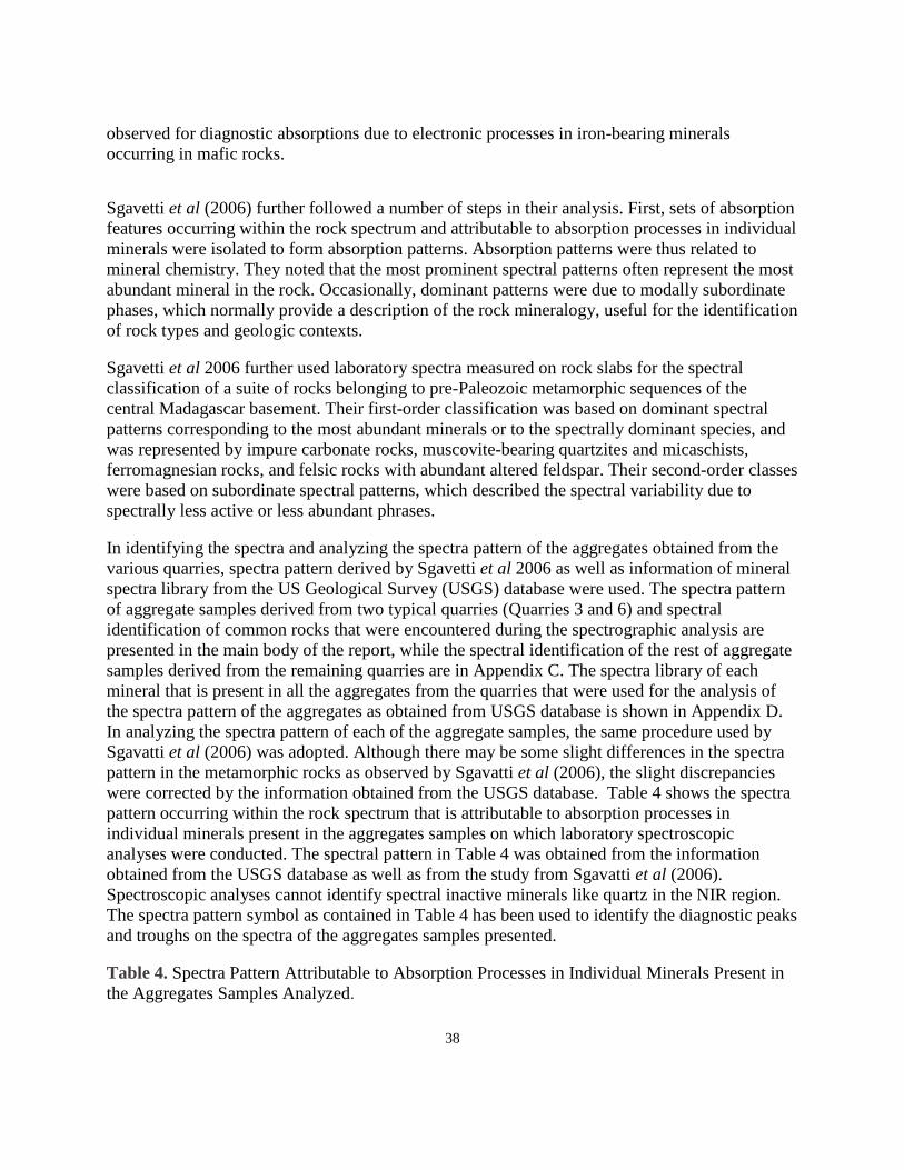
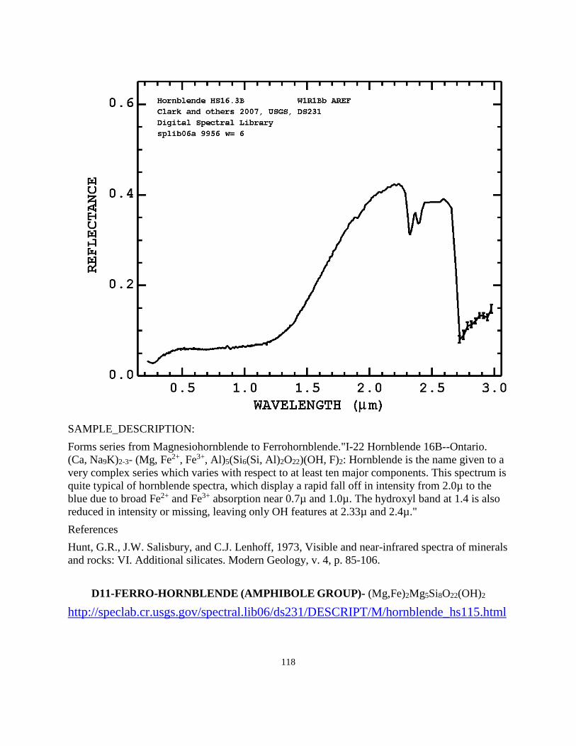
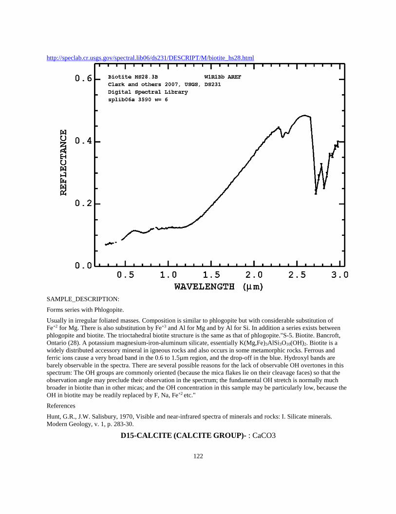
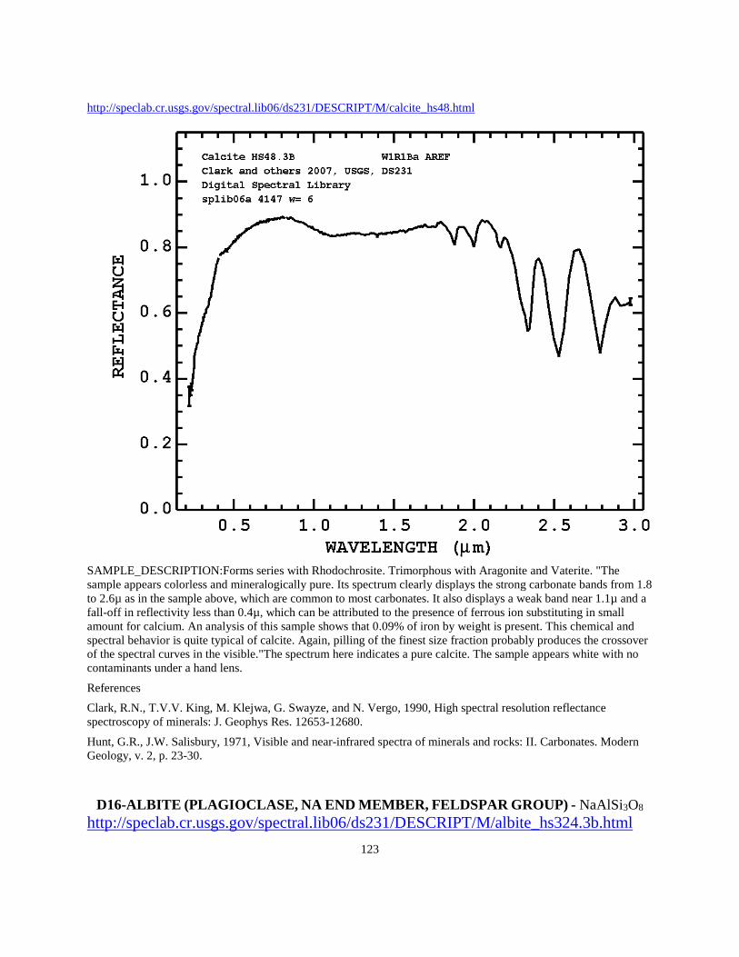
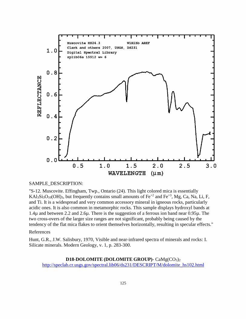
observed for diagnostic absorptions due to electronic processes in iron-bearing minerals occurring in mafic rocks. Sgavetti et al (2006) further followed a number of steps in their analysis. First, sets of absorption features occurring within the rock spectrum and attributable to absorption processes in individual minerals were isolated to form absorption patterns. Absorption patterns were thus related to mineral chemistry. They noted that the most prominent spectral patterns often represent the most abundant mineral in the rock. Occasionally, dominant patterns were due to modally subordinate phases, which normally provide a description of the rock mineralogy, useful for the identification of rock types and geologic contexts. Sgavetti et al 2006 further used laboratory spectra measured on rock slabs for the spectral classification of a suite of rocks belonging to pre-Paleozoic metamorphic sequences of the central Madagascar basement. Their first-order classification was based on dominant spectral patterns corresponding to the most abundant minerals or to the spectrally dominant species, and was represented by impure carbonate rocks, muscovite-bearing quartzites and micaschists, ferromagnesian rocks, and felsic rocks with abundant altered feldspar. Their second-order classes were based on subordinate spectral patterns, which described the spectral variability due to spectrally less active or less abundant phrases. In identifying the spectra and analyzing the spectra pattern of the aggregates obtained from the various quarries, spectra pattern derived by Sgavetti et al 2006 as well as information of mineral spectra library from the US Geological Survey (USGS) database were used. The spectra pattern of aggregate samples derived from two typical quarries (Quarries 3 and 6) and spectral identification of common rocks that were encountered during the spectrographic analysis are presented in the main body of the report, while the spectral identification of the rest of aggregate samples derived from the remaining quarries are in Appendix C. The spectra library of each mineral that is present in all the aggregates from the quarries that were used for the analysis of the spectra pattern of the aggregates as obtained from USGS database is shown in Appendix D. In analyzing the spectra pattern of each of the aggregate samples, the same procedure used by Sgavatti et al (2006) was adopted. Although there may be some slight differences in the spectra pattern in the metamorphic rocks as observed by Sgavatti et al (2006), the slight discrepancies were corrected by the information obtained from the USGS database. Table 4 shows the spectra pattern occurring within the rock spectrum that is attributable to absorption processes in individual minerals present in the aggregates samples on which laboratory spectroscopic analyses were conducted. The spectral pattern in Table 4 was obtained from the information obtained from the USGS database as well as from the study from Sgavatti et al (2006). Spectroscopic analyses cannot identify spectral inactive minerals like quartz in the NIR region. The spectra pattern symbol as contained in Table 4 has been used to identify the diagnostic peaks and troughs on the spectra of the aggregates samples presented. Table 4. Spectra Pattern Attributable to Absorption Processes in Individual Minerals Present in the Aggregates Samples Analyzed.
39
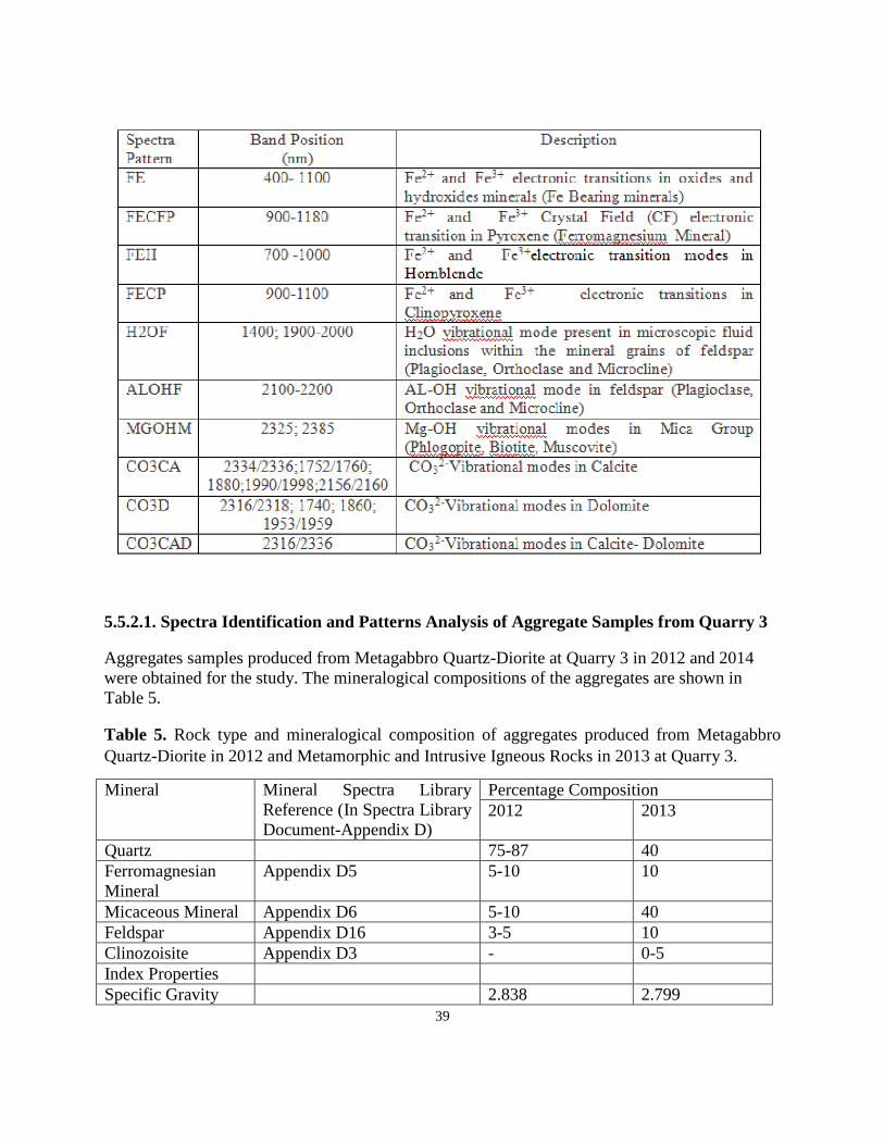
5.5.2.1. Spectra Identification and Patterns Analysis of Aggregate Samples from Quarry 3 Aggregates samples produced from Metagabbro Quartz-Diorite at Quarry 3 in 2012 and 2014 were obtained for the study. The mineralogical compositions of the aggregates are shown in Table 5. Table 5. Rock type and mineralogical composition of aggregates produced from Metagabbro Quartz-Diorite in 2012 and Metamorphic and Intrusive Igneous Rocks in 2013 at Quarry 3.
Mineral Mineral Spectra Library Reference (In Spectra Library Document-Appendix D)
Percentage Composition 2012 2013
Quartz 75-87 40 Ferromagnesian Mineral
Appendix D5 5-10 10
Micaceous Mineral Appendix D6 5-10 40 Feldspar Appendix D16 3-5 10 Clinozoisite Appendix D3 - 0-5 Index Properties Specific Gravity 2.838 2.799
40
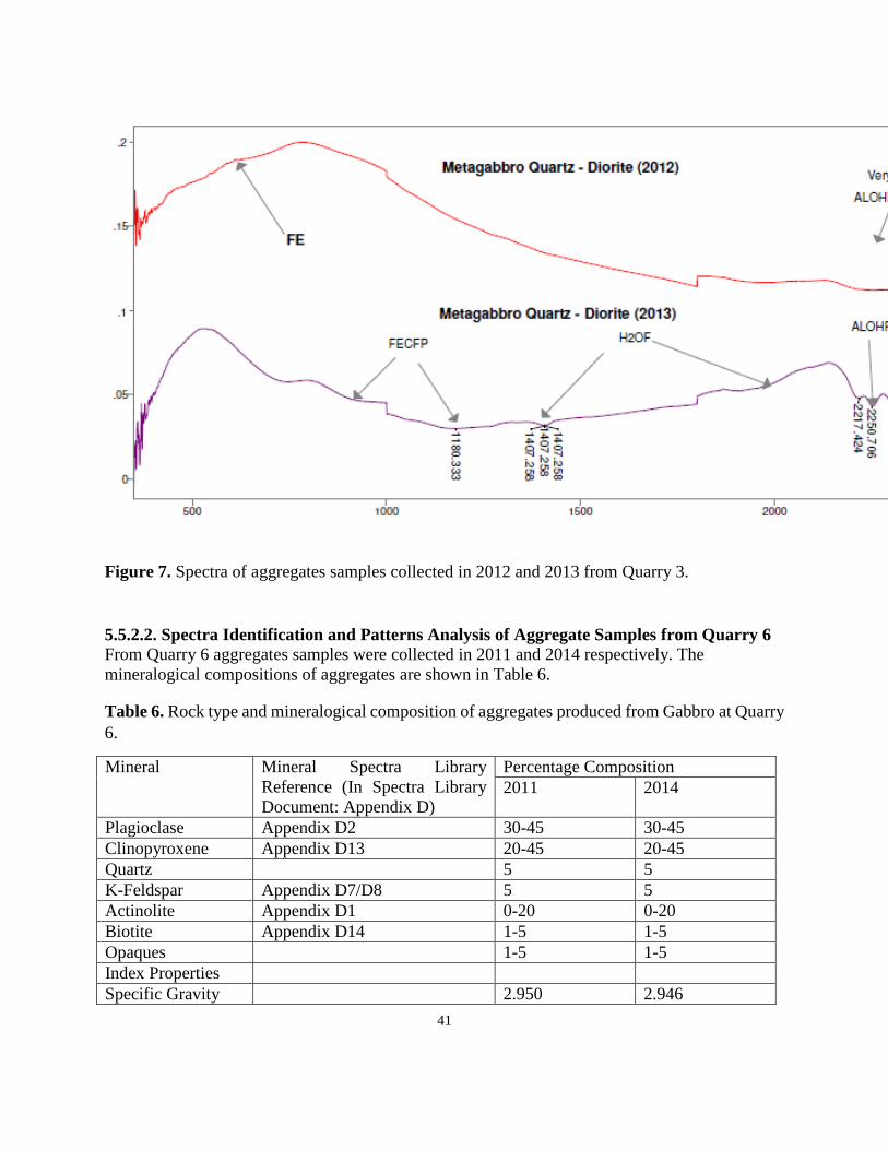
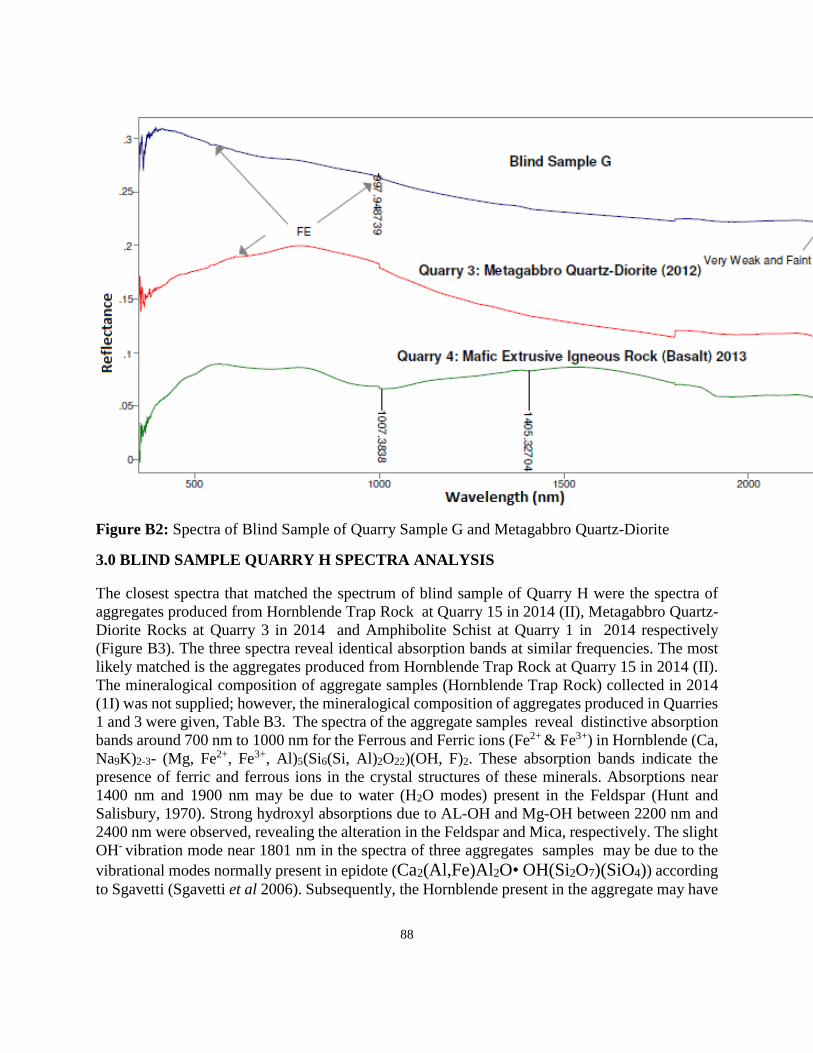
LA (%) 14 15 Friction Category HDFV-III HDFV-III Figure 7 shows the spectra of aggregates samples collected in 2012 and 2013 from Quarry 3. The spectra of the aggregates samples shown are in reflectance and corresponding absorptions wavelength positions are given in nanometer on each spectra. The spectrum of the aggregate collected in 2012 is on top of the stack and it reveals a distinctive absorption wavelength of about 615 nm for the Ferric ions (Fe2+& Fe3+) which is an indication of the Ferromagnesian Mineral (Pyroxene) present in the aggregate. Quartz, which is not spectrally active, constitutes a greater percentage of the minerals present. At around 2400 nm wavelength very weak and faint hydroxyl (OH) combinations in Mica and Feldspar are manifested, which are the reflection of the low composition of Mica (5-10%) and Feldspar (3-5%) present in the aggregate. However, the spectra pattern of the aggregate sample collected in 2013 from the same quarry is significantly different. The major minerals present in the aggregates are spectrally active: Micaceous Minerals (40%), Feldspar (10%), and Ferromagnesian Mineral (10%). These combinations of the spectrally active minerals are manifested in the distinctive absorption bands associated with these minerals. Fe2+ Crystal Field (CF) Electronic transitions in Ca-rich Pyroxene (Ferromagnesian Mineral) are manifested near 944 nm and 1180 nm respectively. The H2O vibrational modes near 1400 nm and 1900 nm respectively suggest the presence of feldspar in the aggregate. The distinctive AL-OH vibrational modes near 2250 nm reveal the incipient alteration of the feldspar. The strong absorption band of Mg-OH vibrational mode near 2354 nm, which are usually present in trioctahedral Mica, suggests the presence of a larger amount of micaceous minerals in the aggregate (40%). Based on the significant differences in the spectra of these two aggregates obtained from the same quarry during different years, there are bound to be differences in their frictional and physical properties (evidenced by the difference in the index properties provided).
41
Figure 7. Spectra of aggregates samples collected in 2012 and 2013 from Quarry 3.
5.5.2.2. Spectra Identification and Patterns Analysis of Aggregate Samples from Quarry 6 From Quarry 6 aggregates samples were collected in 2011 and 2014 respectively. The mineralogical compositions of aggregates are shown in Table 6. Table 6. Rock type and mineralogical composition of aggregates produced from Gabbro at Quarry 6.
Mineral Mineral Spectra Library Reference (In Spectra Library Document: Appendix D)
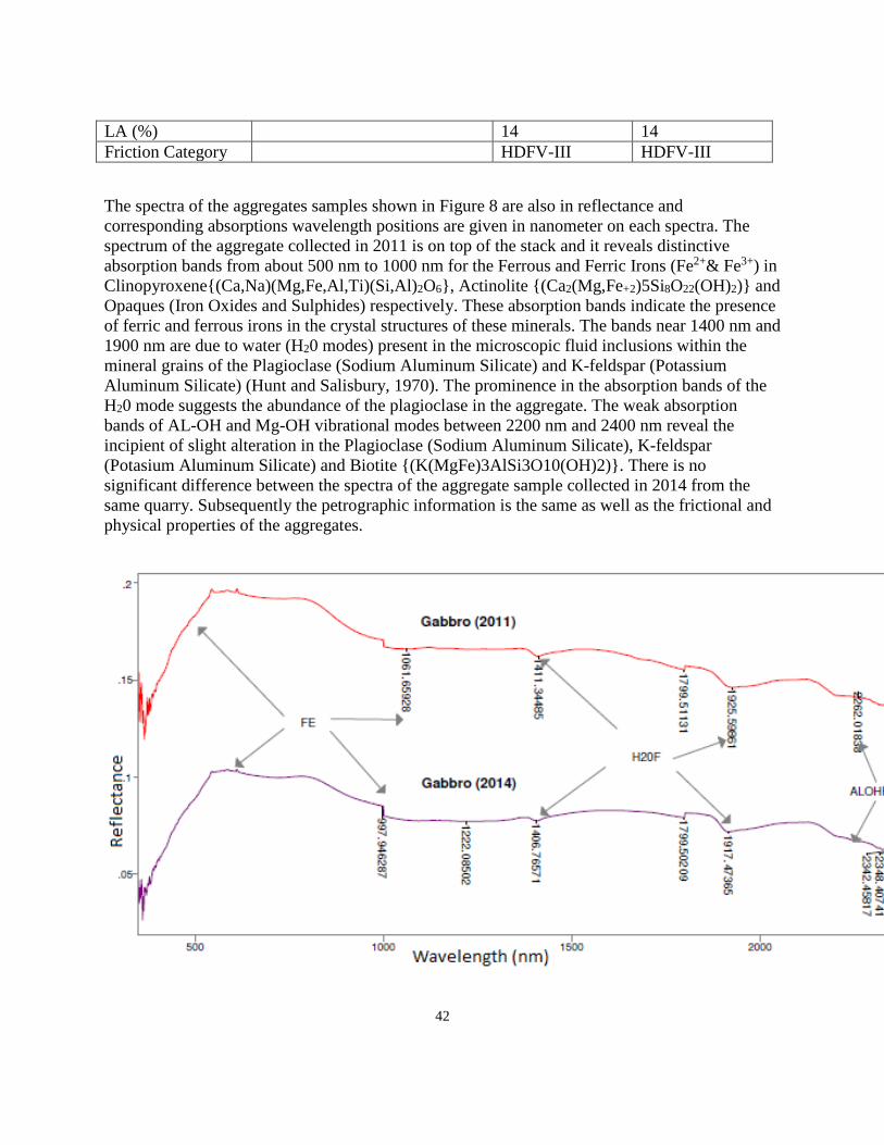
LA (%) 14 14 Friction Category HDFV-III HDFV-III The spectra of the aggregates samples shown in Figure 8 are also in reflectance and corresponding absorptions wavelength positions are given in nanometer on each spectra. The spectrum of the aggregate collected in 2011 is on top of the stack and it reveals distinctive absorption bands from about 500 nm to 1000 nm for the Ferrous and Ferric Irons (Fe2+& Fe3+) in Clinopyroxene{(Ca,Na)(Mg,Fe,Al,Ti)(Si,Al)2O6}, Actinolite {(Ca2(Mg,Fe+2)5Si8O22(OH)2)} and Opaques (Iron Oxides and Sulphides) respectively. These absorption bands indicate the presence of ferric and ferrous irons in the crystal structures of these minerals. The bands near 1400 nm and 1900 nm are due to water (H20 modes) present in the microscopic fluid inclusions within the mineral grains of the Plagioclase (Sodium Aluminum Silicate) and K-feldspar (Potassium Aluminum Silicate) (Hunt and Salisbury, 1970). The prominence in the absorption bands of the H20 mode suggests the abundance of the plagioclase in the aggregate. The weak absorption bands of AL-OH and Mg-OH vibrational modes between 2200 nm and 2400 nm reveal the incipient of slight alteration in the Plagioclase (Sodium Aluminum Silicate), K-feldspar (Potasium Aluminum Silicate) and Biotite {(K(MgFe)3AlSi3O10(OH)2)}. There is no significant difference between the spectra of the aggregate sample collected in 2014 from the same quarry. Subsequently the petrographic information is the same as well as the frictional and physical properties of the aggregates.
43
Figure 8. Spectra of aggregates samples collected in 2011 and 2014 from Quarry 6.
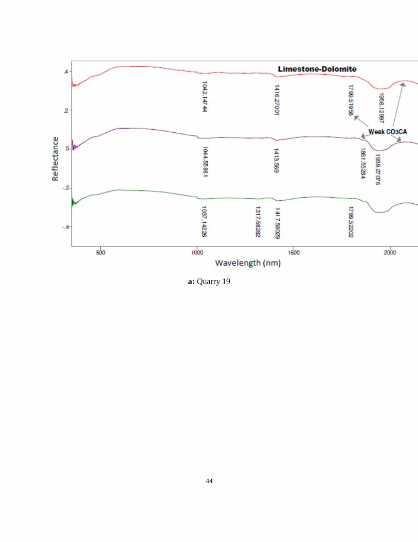
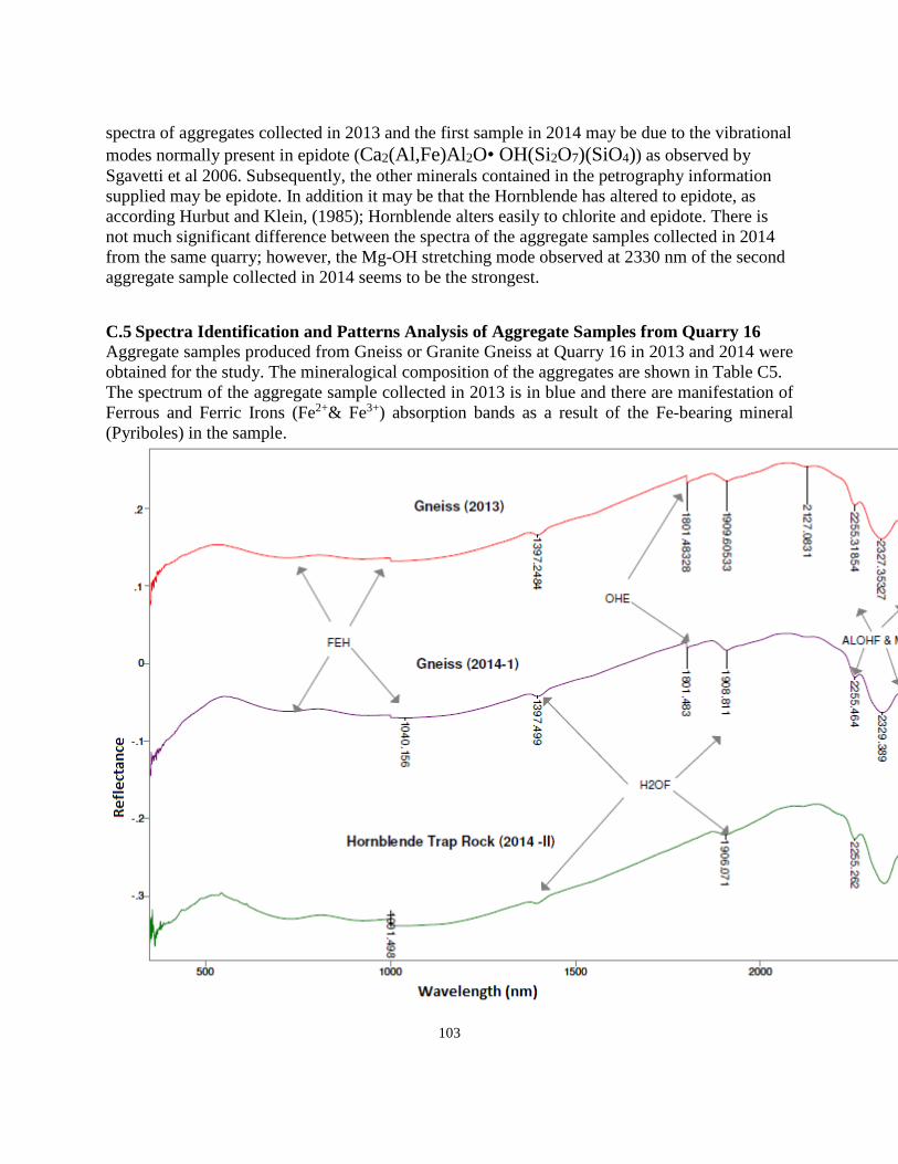
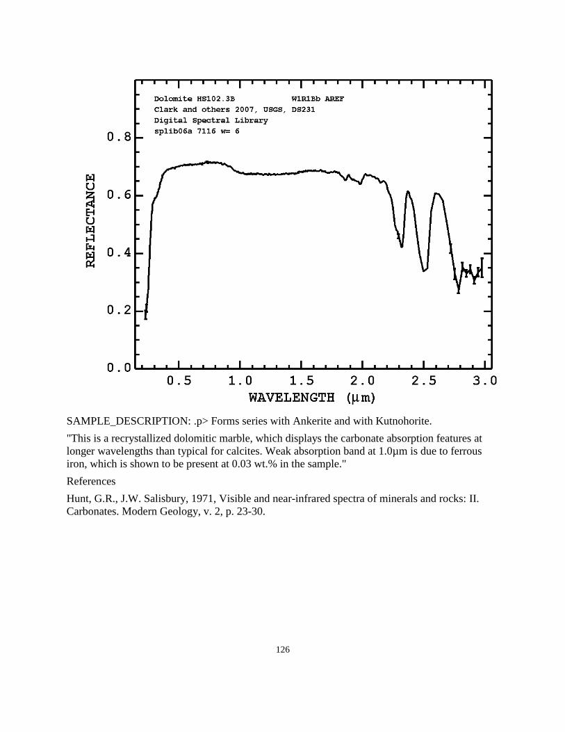
5.5.2.3 Spectra Identification of Common Rocks Encountered (Limestone-Dolomite and Limestone) From all the quarries, multiple spectra for a particular rock are put together, in order to aid aggregate source validation. From all the quarries the following rock types are derived from more than one quarry: Limestone-Dolomite (Quarry 19 & 20), Limestone (Quarry 7, 9, 17, 18, 21, 22, 23, & 24) 5.5.2.3.1 Spectra Identification and Patterns Analysis of Aggregates Produced from Limestone Dolomite (Quarry 19 & 20) The samples were collected in 2009, 2010, and 2012 from Quarry 19 and in 2009 and 2010 from Quarry 20 respectively and the rock type is Limestone-Dolomite which comprises mostly of calcite (CaCO3) and Dolomite (CaMg(CO3)2). The spectra of the five samples are shown in Figure 9. Weak Ferric and ferrous absorption bands around the visible range at 1000 nm reveals the presence of ferrous ions substituting in small amount of calcium. The spectra clearly displays strong carbonate band (CO3
2-) normally present in combination of Calcite (CaCO3) and Dolomite (CaMg(CO3)2 at 2329 nm. In addition there are weak bands of carbonate at 1804 nm and 2147 nm respectively, which are typical of calcite minerals. The prominence of the absorption bands of the Calcite mode suggests the abundance of the calcite-dolomite in the aggregate. There are no significant differences in all the spectra.
44
a: Quarry 19
45
b: Quarry 20
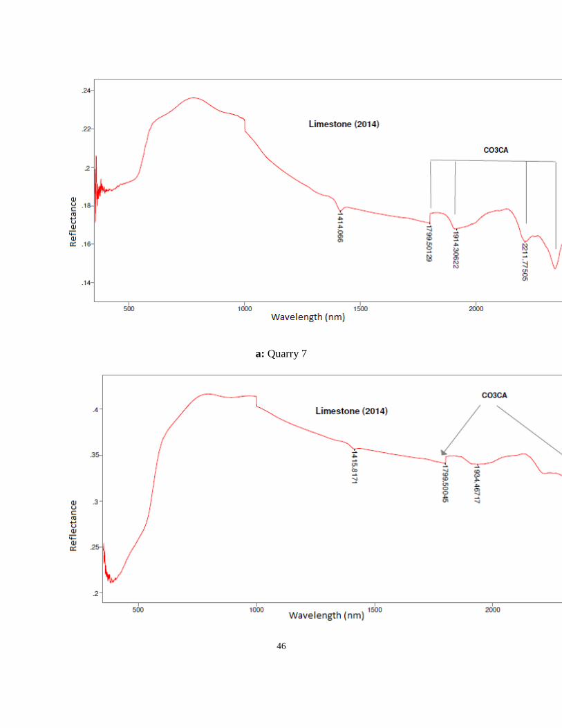
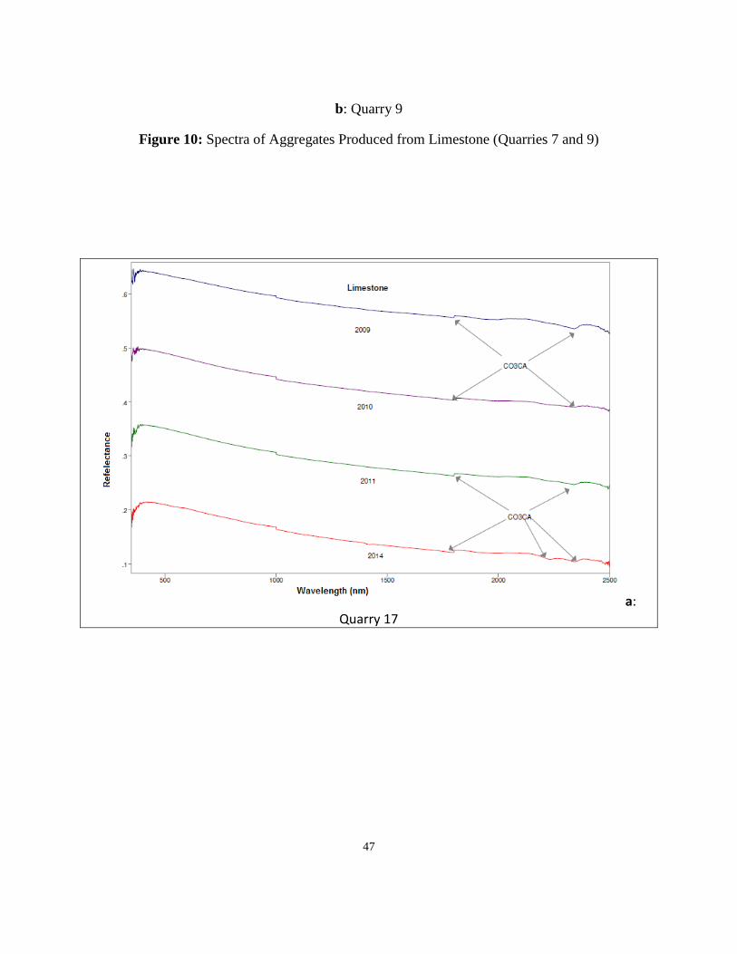
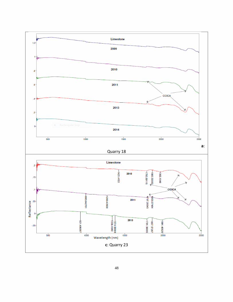
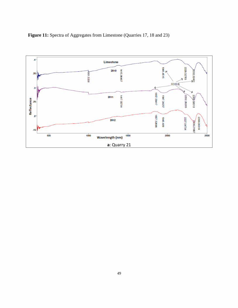
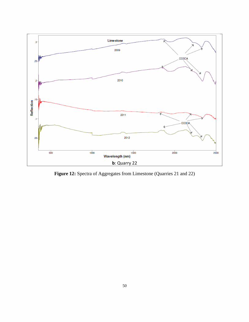
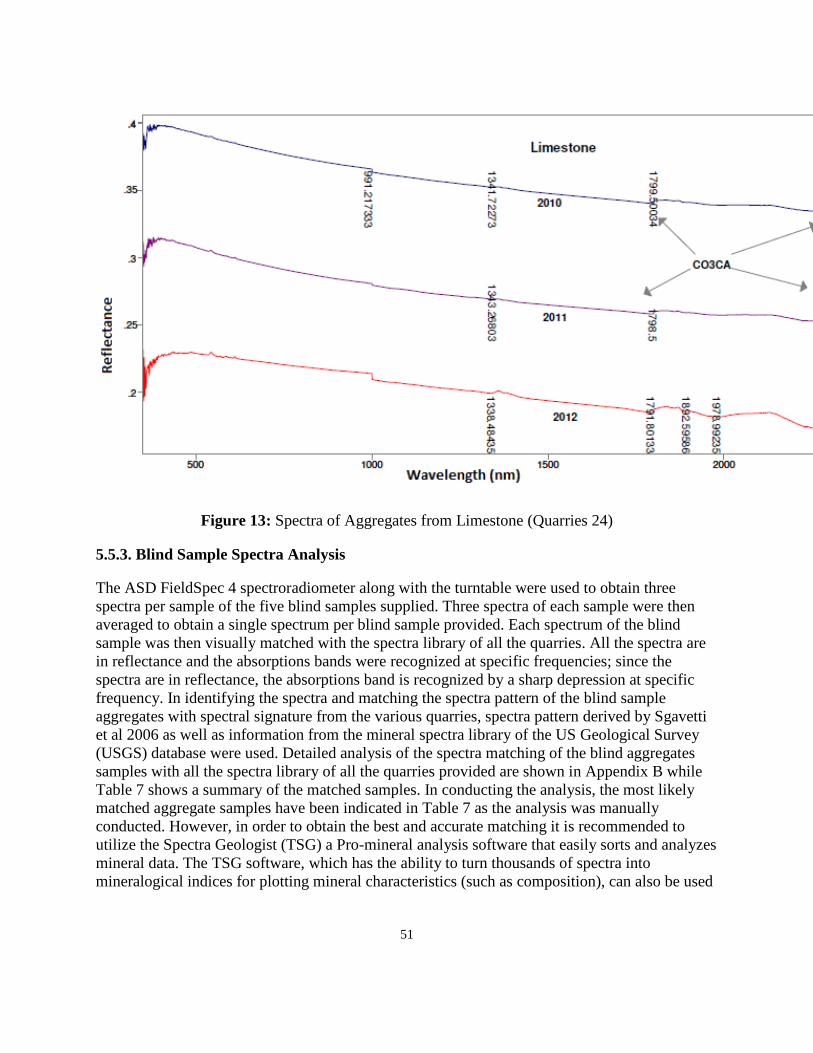
Figure 9: Spectra of Aggregates Produced from Limestone Dolomite (Quarry 19 & 20). 5.5.2.3.2 Spectra Identification and Patterns Analysis of Aggregates Produced from Limestone (Quarry 7, 9, 17, 18, 21, 22, 23 & 24) Figures 10-13 show four distinctive spectra of aggregates produced from Limestone sampled during different years from eight quarries (Quarries 7, 9, 17, 18, 21, 22, 23 and 24) as follows: (1) Figure 10; Quarries 7 and 8, (2) Figure 11; Quarries 17, 18 and 23, (3) Figure 12; Quarries 21 and 22 and (4) Figure 13; Quarry 24. The year of collection and quarry location are shown in the figures. Weak Ferric and ferrous absorptions bands at around the visible range from about 400 nm to 1000 nm reveal the presence of ferrous impurities in the limestone. The spectra clearly display strong carbonate bands (CO3
2-) normally present in Calcite (CaCO3) at 1800 nm, 2200 nm and 2340 nm, respectively. The prominence of the absorption bands of the Calcite mode suggests the abundance of the calcite in the aggregates. The spectra also show another weak Carbonate band at 1847 nm.
46
a: Quarry 7
47
b: Quarry 9
Figure 10: Spectra of Aggregates Produced from Limestone (Quarries 7 and 9)
a: Quarry 17
48
a: Quarry 18
c: Quarry 23
49
Figure 11: Spectra of Aggregates from Limestone (Quarries 17, 18 and 23)
a: Quarry 21
50
b: Quarry 22
Figure 12: Spectra of Aggregates from Limestone (Quarries 21 and 22)
51
Figure 13: Spectra of Aggregates from Limestone (Quarries 24)
5.5.3. Blind Sample Spectra Analysis The ASD FieldSpec 4 spectroradiometer along with the turntable were used to obtain three spectra per sample of the five blind samples supplied. Three spectra of each sample were then averaged to obtain a single spectrum per blind sample provided. Each spectrum of the blind sample was then visually matched with the spectra library of all the quarries. All the spectra are in reflectance and the absorptions bands were recognized at specific frequencies; since the spectra are in reflectance, the absorptions band is recognized by a sharp depression at specific frequency. In identifying the spectra and matching the spectra pattern of the blind sample aggregates with spectral signature from the various quarries, spectra pattern derived by Sgavetti et al 2006 as well as information from the mineral spectra library of the US Geological Survey (USGS) database were used. Detailed analysis of the spectra matching of the blind aggregates samples with all the spectra library of all the quarries provided are shown in Appendix B while Table 7 shows a summary of the matched samples. In conducting the analysis, the most likely matched aggregate samples have been indicated in Table 7 as the analysis was manually conducted. However, in order to obtain the best and accurate matching it is recommended to utilize the Spectra Geologist (TSG) a Pro-mineral analysis software that easily sorts and analyzes mineral data. The TSG software, which has the ability to turn thousands of spectra into mineralogical indices for plotting mineral characteristics (such as composition), can also be used
52
to determine the mineralogical composition (qualitative and quantitative) of the aggregates blind samples. Unfortunately Morgan State University has not yet acquired this software.
53
Table 7. Summary of Blind Samples Matching.
Blind Sample Quarry
Matching Quarry/Rock Type (Most Likely)
Quarry/Rock Type (Likely)
1 2 3
A Quarry 3 (2014) Metagabbro Quartz-Diorite
Quarry1 2014 Amphibolite Schist
Quarry 15 2014-1 Gneiss
Quarry 3 (2013) Metamorphic and Intrusive Igneous Rocks
G Quarry 3 (2012) Metagabbro Quartz-Diorite
Quarry 4 2013 Mafic Extrusive Rock (Basalt)
H Quarry 15 2014 (II) Hornblende Trap Rock
Quarry 3 (2014) Metagabbro Quartz-Diorite
Quarry 1 2014 Amphibolite Schist
Quarry 3 2013 Metamorphic and Igneous Rocks
K Quarry 13 2013 Quartz Plagioclase Gneiss-Granite Gneiss
5.6. Chemometrics Results and Conclusions Discriminant analysis, based on Mahalanobis Distances calculated from reflectance data at full wavelengths (400-2450 nm) was also able to discriminate limestone found in a particular quarry from other aggregates derived from other quarry locations. When applied to a validation set, the two classification models developed correctly classified 100% of aggregate samples as not from the sample population. However, it was not possible to perform the discriminate analysis in order to determine the origin of the blind samples given because there was not sufficient variability in aggregate samples from the non-carbonate quarries. Most non-carbonate quarries have samples collected from one or two locations from each quarry; however, in order to incorporate variability and generate a good classification model at least samples must be collected from
54
about five different locations with varying geomorphology within a quarry. Additionally, the quantitative analysis of the physical properties of the aggregates that was carried out with the Chemometric software was suspended because there were not sufficient samples from different locations within the quarries that could have generated accurate quantitative models. The results obtained so far from the spectra identification and pattern analysis showed promise for the utilization of NIR spectroscopy for detecting and explaining the variability in the frictional and physical properties of aggregates within a quarry over a period of time. Subsequently, the spectra obtained for the various aggregates can be used as diagnostic tools to validate an aggregate source. The GRAMS IQ software has the capability of combining and incorporating both the qualitative and quantitative models in an automated system that screens/classifies the aggregates and predicts the frictional parameters that are required for QA and QC of HMA surface mix aggregates in real time. From the results of the spectra analysis and absorption variability, it can be concluded that the spectra pattern can be used to explain the variation in the frictional and physical properties of aggregates within a quarry from one location to the other. In addition, the basis for the identification of the diagnostic features of the minerals and ions has been given in Table 4 as well as from information from the spectral library of the associated minerals in the USGS database (Appendix D). The absorption pattern of the signature of the aggregates is related to the chemical composition of the aggregates; however, it was not possible to identify the presence of quartz as the mineral is not spectrally active in the NIR region. In identifying the source of the aggregate blind samples the most likely matched aggregates were visually obtained by inspection; however in order to obtain the best and accurate matching it is recommended to utilize the Spectra Geologist (TSG) a Pro-mineral analysis software that easily sorts and analyzes mineral data. The TSG software can also be used to determine the mineralogical composition of any blind aggregate sample as well as to analyze and visualize the mineralogy of large data sets.
55
6.0. NEURAL NETWORK METHOD 6.1. NN Overview The Neural Network (NN) Method is based on a statistical mapping between a set of inputs and a set of outputs. In the current implementation, the 2500 spectral components of each aggregate sample were parametrically reduced into a 25th–order model, which has been shown to provide good performance on the current aggregate quarry set. This is illustrated in Figure. 14. FIG. XXXXX Aggregate 3A1, original spectrum and the 25th –order model spectrum The 25 model coefficients then form the input data to the neural network. The order of the model can be increased, or decreased, as appropriate. The output parameters are the Specific Gravity (SG), LA coefficient (LA), and the Friction Category (FC). The number/type of output parameters can be changed but this must be done prior to network training. In this methodology, processing is done in two(2) phases. Phase I is a training phase, where the processing engine is trained to estimate Specific Gravity, LA, and Friction Category by Figure 14. Aggregate 3A1, Original Spectrum & the 25th –Order Model Spectrum. The 25 model coefficients then form the input data to the neural network. The order of the model Figure 14. Aggregate 3A1, Original Spectrum & the 25th –Order Model Spectrum. The 25 model coefficients then form the input data to the neural network. The order of the model can be increased, or decreased, as appropriate. The output parameters are the Specific Gravity (SG), LA coefficient (LA), and the Friction Category (FC). The number/type of output parameters can be changed but this must be done prior to network training. 6.2. NN Analysis In this methodology, processing was done in two (2) phases. Phase I was a training phase, where the Processing Engine was trained to estimate SG, LA, and FC by recursively trying to achieve a best fit between the true values and the NN’s estimated outputs. The NN’s internal processing weights were adjusted on each iteration until either a certain number of training iterations was
56
reached, or, there was some minimum difference between the true aggregate parameter values and the estimated values. Phase II was the classification phase, in which the 25 model parameters estimated from the spectrophotometer spectrum of an (unknown) aggregate sample were input to the trained Processing Engine, i.e., the trained neural network, and the network estimated the SG, LA, and FC. A Block diagram of the ‘Phase I – Training Phase’ is illustrated graphically below in Figure 15, and for ‘Phase II – Estimation Phase’ in Figure 16.
Phase I – Training Phase
Figure 15. NN Method Training Phase.
Phase II – Estimation Phase
Figure 16. NN Method Estimation Phase. The basic algorithm flow is as follows: A) Phase I – Training Phase 1 – An Excel spreadsheet was generated which consisted of 25-coefficient vectors, one for each measured aggregate sample (Figure 17). This was the NN method training input data. 2 – A matching target vector was generated. The current implementation utilized two target vectors: one for the Friction Category, and a second for the SG, LA Coefficient (Figure 15). B) Phase II – Estimation Phase 1 – An aggregate sample spectrum was recorded with the FS4 Spectroradiometer, 2 – 25 spectrum estimation coefficients were extracted (this was done automatically in the Processing Engine), 3 – The coefficients were then sent to the Processing Engine for parameter estimation, and 4 – The estimated values of SG, LA coefficient, and FC were then obtained.
57
Figure 17. Illustration of the NN Matrix of Input Data Vectors.
Figure 18. Illustration of the Partial Contents of the Estimator NN Target Data File. 6.3. NN Results and Conclusions Table 8 Iilustrates the results obtained by the ‘Aggregate Characteristics Estimator’ after the network was trained for aggregate samples across the six friction categories. As noted there were no samples for friction category 4. Table 9 illustrates the results obtained for the GIS Lab’s ‘unknown’ aggregate No. 26.
58
59
Table 8. Test Results for the Full FC/SG/LA Estimator.
26 ‘unknown’ 5 ‘unknown’ 2.577 ‘unknown’ 20.6125 6.4. SHA Aggregate Blind Test Results using NN The Maryland SHA delivered aggregate samples from five quarries to Morgan State. The aggregate spectra were extracted using the FS4. Ten spectra were collected and then averaged, and 3 averaged spectra samples per quarry were then used for this analysis (see FS4 setup in Figure 2). The aggregate samples for the Blind Test data files were denoted as QA, QG, QH, QK, and QS (Q is for quarry, and A, G, H, K, and S are identification letters). The NN method depends on a classification network which has been trained on the class of data for which it will eventually be able to blindly classify. The robustness of the network depends on several factors – the quantity of data, which should span the extremes of each class of data, the variance of the data within a particular class and the separation between the classes, i.e. preferably orthogonal, with no overlap. First Trial The following results were obtained by processing the first column of spectra data in each of the five Quarry data files. Additionally, a 4th column of spectrum data was synthesized as the average spectrum of the particular quarry by averaging the measurement data from the first three spectra for that quarry. I.e., ‘Qx_Col1.txt’ are the estimation results obtained using the first column/spectra data and ‘Qx_Avg.txt’ are the estimation results using the averaged *input* spectra (NOT the average of the three estimation output results).
60
Table 10. Parameter Estimation Results Using the Original Raw Spectra Measurements. Estimates obtained using ‘Col1’ and ‘Ave’ data only).
Aggregate File Estimated Friction
Class Estimated Specific
Gravity Estimated LA
Coeff. QA_Col1.txt 5 2.8211 17.7471 QA_Avg.txt 3 2.7260 18.6891 QG_Rb_Col1.txt 6 2.4431 36.9904 QG_Rb_Avg.txt 6 2.3566 31.1416 QH_Col1.txt 5 2.5446 15.3972 QH_Avg.txt 3 2.8718 10.9863 QK_Col1.txt 5 2.9454 20.6246 QK_Avg.txt 5 3.0059 17.0632 QS_Col1.txt 3 2.8919 16.5478 QS_Avg.txt 5 3.1472 9.9801 Though this is a blind test, from prior performance of the estimator it was evident that some factor is causing a significant amount of variance in the estimates, i.e., the estimation of two different friction classifications (samples QA, QH, and QS) using the raw 1st column input spectra measurement, and the input data averaged over the three columns of input measurement data. Trial 2 In trial two, the remaining two sample measurements, i.e., measurements ‘2’ and ‘3,’ from each quarry were used to provide additional parameter estimates for that particular quarry. This was done for all five quarries. The following table illustrates the original results obtained using measurements ‘1’ (i.e., ‘Col1’ data) and ‘Ave,’ along with the estimation results utilizing measurements ‘2’ and ‘3’ for each quarry. Trial 3 In trial three, the first 50 wavelength samples, which were extremely noisy and showed very little correlation across the three measurements-per-sample, were excised from each measurement file. This is the variance that can be seen across the estimates in Trial 1, as the model tried to estimate not only valid data, but also noise. As in Trial 2, parameter estimations are performed for each of the three samples-per-quarry. As in prior cases an additional estimate is made utilizing an average spectrum input vector. The results are shown in the following table. Trial 4 Similarly to Trial 3, the first few noisy samples were excised. Additionally, the last few noisy samples were also excised. The original data spanned 350 <= λ <= 2500. In Trial 4, the excised data spanned 400 <= λ <= 2450. Trials ‘3’ and ‘4’ were performed in an attempt to reduce the overall variance of the Specific Gravity, LA Coefficient, and Friction Category estimates, for the same sample.
61
Compiled SHA Aggregate Blind Test Results The compiled results of the SHA Blind Tests Results are given in Table 11 below. Table 11. Compilation of Results of SHA Blind Tests. Quarr
Note: ‘Trial 2’ is not included as the Trial 1 and Trial 2 results for the ‘Average Input Spectrum’ are identical. Trial 2 just added the results for aggregate samples 2 and 3. I.e., those results are illustrated in Table 10. ‘Sanity Check’ Due to what seemed as fairly high variance on the estimation results for same-quarry aggregates a sanity check on the Neural Network Method was performed using three different samples from Quarry 18. The results are illustrated in Table 12.
62
Table 12. Parameter Estimation Results, Original Quarry 18A Data.
Aggregate File
True Friction Category
Estimated Friction Category
True Specific Gravity
Estimated Specific Gravity
True LA Coefficien
t
Estimated LA
Coefficient
c:\18A1.txt 5 5 2.65 2.6495 21 21.0046 c:\18A2.txt 5 5 2.65 2.6408 21 20.6631 c:\18A3.txt 5 5 2.65 2.6531 21 21.0912 7.0. SPECTRAL LIBRARY DEVELOPMENT The MSU GIS Laboratory received 42 aggregate samples from 19 different quarries. The information provided with each aggregate consisted of the aggregate producer, quarry name, friction category, year sampled, rock type, specific gravity, LA coefficient, micro deval, SS, BPN, avg. AIR, and mineral/% Composition. While not all parameters were available for every aggregate sample, specific gravity and LA coefficients were available for most. This information formed the basis for constructing the spectral library.
Figure 19. Main Page of MSU-GIS Laboratory Digital Spectral Library website. Figure 19 illustrates the opening page of the MSU-GIS Laboratory Digital Spectral Library website. The current logo is a temporary place holder. There are four main columns with the left-most column containing the name of the aggregate producer, quarry, and date on which the aggregate was sampled. The right-most three columns are hot-linked to the appropriate location to obtain either the desired aggregate description, data, or plot. For each additional entry to the
63
Library, on a new row the aggregate producer, quarry, and sample date information is entered into the left-most column. Then, a description file, ASCII data file, and spectral plot file are created and added to their appropriate directories. The names of the associated description, ASCII data, and spectral plot files are entered into columns 2, 3, and 4, respectively. These filenames are then hot-linked to the respective file location.
Figure 20. Underlying Data Structure of the Spectral Library. Figure 20 illustrates the primary underlying data structure. File folder ‘Aggregate Descriptions’ contains the .txt files describing various attributes of the associated aggregate. There is an ‘Aggregate Description Template’ which can be used when adding new aggregates. Folder ‘Aggregate ASCII Data’ contains .txt files whose content is two columns of data. The left column is wavelength which spans 350 – 2500 nm. The right column contains the values of average reflectance for the associated wavelength. The single column of average reflectance data is derived by averaging the three epochs of reflectance data contained in the original data file associated with the particular aggregate sample. The ‘Aggregate Spectrums’ folder contains the spectrum derived from the aggregate average reflectance data contained in the ‘Aggregate ASCII Data’ file. Any time a new aggregate is measured, a new text description file, text ASCII data file, and JPEG spectrum file should be generated and saved to the appropriate folder. The final folder ‘Templates’ contains the main website file. Any time a new aggregate is measured a new row should be added to the Library homepage, as described previously. The main website file is developed in Adobe Dreamweaver CS5.5.
64
Figure 21. Structure of the ‘Aggregate ASCII Data’ file folder.
Figure 21 illustrates the file structure of the ‘Aggregate ASCII Data’ file folder. The files are .txt format and named to illustrate that they contain data which is the average reflectance of the three columns of data contained in the original aggregate data files (Note that the file named ‘17A_Avg_17B_Avg_17C_AVG&17D_A..’ was just a test file, and is not used in the actual library).
65
Figure 22. Segment of an Excel file used to generate the average spectrum. Figure 22, above, illustrates how the data from aggregate sample 03A measurement epochs 1, 2, and 3 (in columns ‘D’, ‘E’, and ‘F,’ respectively) are used to form the average spectral response which is given in column ‘B.’ I.e., the contents of cell B1 are calculated as, B1 = 1/3 * (D1 + E1 + F1) ……………. (6) The remaining cells, i.e., B2, B3, …., B2151 are calculated in a like manner.
Figure 23. Illustration of the Contents of the ‘Aggregate Descriptions’ file folder. The contents of the folder are .txt files and an example of the contents of a description file is shown in Figure 23: DATE: 09/04/15 SAMPLE NAME/CODE: 03A AGGREGATE PRODUCER: Company 03A QUARRY NAME: ‘ABC FRICTION CATEGORY: HDFV-III SAMPLE COLLECTION DATE: 2014 ROCK TYPE: Metagabbro Quartz - Diorite SPECIFIC GRAVITY: 2.212 LA: 12 MINERALOGICAL COMPOSITION: Quartz (75-87%) Micaceous Min (10-20%)/Feldspar (3-15%) CURRENT SAMPLE LOCATION: GIS Laboratory, Morgan State University, RM: CBEIS ULTIMATE SAMPLE LOCATION: Maryland State Highway Administration SAMPLE DESCRIPTION:
66
IMAGE OF SAMPLE: An example of the ‘Sample Description’ file (Template developed after that used by the USGS). The ‘Aggregate Spectrums’ file folder content format is shown below. Spectrums are currently saved as JPEG images generated either by ENVI, or a combination of Microsoft EXCEL and Microsoft Notepad. All the example spectrums listed in Figure 24 were generated and formatted in the Microsoft environment.
Figure 24. Illustration of the ‘Aggregate Spectrums’ file naming conventions. A sample of the contents of a spectrum file, i.e., ‘03A_AVG_Spectrum,’ is illustrated below in Figure 25.
67
Figure 25. Aggregate Sample 03A_AVG_Spectrum.
Figure 26. Contents of the ‘Templates’ File Folder. Figure 26 illustrates the contents of the ‘Templates’ folder which contains the GIS main website page ‘GIS_MainPage,’ and a ‘placeholder’ site logo. The site will currently run in ‘Local’ mode by opening a browser, then ‘File’ - - - > ‘Open File’ and navigating to, and double-clicking on ‘GIS_Main Page.’ Note, however, that as currently implemented the directory structure illustrated in Figure 15 must be maintained; i.e., the best way to effect this is to copy and paste the top folder – in this example, ‘Amalfi_Wilson_Spectral
68
Library,’ which contains all of the other folders. Other than adding more aggregate data, and maintaining the database, the remaining task is to obtain hosting on, i.e., Morgan State University’s server. 8.0. RESEARCH FINDINGS/DISCUSSION 8.1. Chemometrics Discriminant analysis, based on MHD calculated from reflectance data at full wavelengths (400-2450 nm) was also able to discriminate limestone found in a particular quarry location from other aggregates derived from other quarry locations. When applied to a validation set, the two classification models developed correctly classified 100% of aggregate samples as not from the sample population. The results obtained so far from the spectra identification and pattern analysis showed promise for the utilization of NIR spectroscopy for detecting and explaining the variability in the frictional and physical properties of aggregates within a quarry over a period of time. Subsequently, the spectra obtained for the various aggregates can be used as diagnostic tools to validate an aggregate source. The GRAMS IQ software has the capability of combining and incorporating both the qualitative and quantitative models in an automated system that screens/classifies the aggregates and predicts the frictional parameters that are required for QA and QC of HMA surface mix aggregates in real time. From the results of the spectra analysis and absorption variability, it can be concluded that the spectra pattern can be used to explain the variation in the frictional, mineroligical and physical properties of aggregates within a quarry from one location to the other. In addition, the basis for the identification of the diagnostic features of the minerals and ions has been given in Table 4 as well as information from the spectral library of the associated minerals in the USGS database. The absorption pattern of the signature of the aggregates is related to the chemical composition of the aggregates; however, it was not possible to identify the presence of quartz as the mineral is not spectrally active in the NIR region. 8.2. Neural Network While the number of aggregate sample spectra was not extensive it can be seen from the results that given only one spectrum measurement the NN can provide outstanding parameter estimation – given that the sample spectrum comes from a population over which the NN was trained. Thus the NN is a viable solution for the desired objective of quick parameter estimation based solely on optical spectrographic measurement. Some of the factors affecting results are due to time and the relatively small numbers of sample spectra per friction category. The NN is a statistical estimator and relies heavily on the variance of the training set, in order to sufficiently estimate data not originally included in the training set. It can be seen from Table 3 that the quantity of training data utilized in Friction Categories ‘1,’
69
‘2,’ and ‘6’ may not have allowed sufficient classification abilities in these three classes. While there was a bit more data for FC categories 3, and 5, the results for samples in those categories would depend on whether the variance of the training data spanned the expected/class values of specific gravities, LA coefficients, and FCs.
• Preliminary results indicate that spectrometric methods could be used to significantly reduce the amount of time spent by the SHA to analyze aggregate samples and extract friction parameters.
• In this particular algorithm, Processing Engine training is the biggest time factor, but training is done off-line.
• After the aggregate spectrum is measured, the remaining steps to parameter estimation can be accomplished on the order of 15 minutes.
9.0. CONCLUSIONS In conclusion, both the Chemometrics and Neural Network (NN) methodologies showed very promising results. The Chemometrics did differentiate limestone from different quarry locations, and was able to validate a higher percentage of aggregates samples as not from the sample population. It was also able to determine the active mineralogical composition of some of the aggregate samples, based on the distinctive absorption bands associated with these minerals. In some cases, the analysis was able to differentiate aggregates from the same quarry which suggested the ability of the Chemometrics methodology being able to function properly when used to validate the source of aggregates used in construction. The NN methodology was extremely quick in estimating aggregate parameters; in some cases, it took just a few minutes including accurate parameter estimates of SG, LA coefficient, and Friction Category. The challenge however, of the NN methodology is that like most statistically based estimators it requires a large dataset, which span the extremes of all the particular classes. This provides sufficient variance within classes, thereby allowing the estimator to accurately predict parameters for spectra which were not included in the training set. It should be noted that the NN training only needs to be done once, unless additional classes/statistics need to be added. In the future, the effects of the model-order parameter, which is used to reduce the number of spectral coefficients used for estimating the aggregate parameters, could be investigated. The Spectral Library is a very beneficial tool that can be easily updated. The architecture consists of four primary entities: 1 – The library ‘Main’ HTML page, 2 – a directory of spectral data files, 3 – a directory of aggregate information, and 4 – a directory of spectral plots. In application it will need to be hosted on a ‘live’ website.
70
REFERENCES
ASD (2007). “Indico Pro User Manual.” ASD Inc. Boulder, CO Document 600235 Rev. D. ASD Inc. www. Asdi.com
ASD (2012). “Chemometrics Training Manual for GRAMS IQ/IQ Predict v9.1”. ASD Inc. Boulder, CO. Document 600065 Rev. A. ASD Inc. www. Asdi.com. ASD Inc. a Panalytical
ASTM D3042-09 (2015). “Standard Test Method for Insoluble Residue in Carbonate Aggregates”. ASTM International, West Conshohocken, PA, 2015.
ASTM E 1911-09 ae1 (2009). “Standard Test Method for Measuring Paved Surface Properties Using the Dynamic Friction Tester”. ASTM International, West Conshohocken, PA, 2009.
Barker, S. and Arnold, T. (2013). “Real-Time Quality Control Monitoring and Characterization of Aggregate Materials in Highway Construction Using Laser Induced Breakdown Spectroscopy”. Transportation Pooled Fund Study Details.
Berg, M.D.V. and Jarrard, R.D. (2002) “Determination of Equatorial Pacific Mineralogy Using Absorption Spectroscopy”. Proceedings of the Ocean Drilling Program, Initial Reports Volume 199
Cheewapramong, P. (2007). “Use of Near-Infrared Spectroscopy for Qualitative and Quantitative Analyses of Grains and Cereal Products”. Doctoral Dissertation, University of Nebraska, Lincoln, NE.
Chesner, W.H. and McMillan, N.J. (2012). “Automated Laser Spectrographic Pattern Matching for Aggregate Identification”. Final Report, National Cooperative Highway Research Program NCHRP IDEA Project 150.
Clark, R.N. (1999): Spectroscopy of Rocks and Minerals and Principles of Spectroscopy, in Remote Sensing for the Earth Sciences, Manual of Remote Sensing 3rd Ed. Vol. 3 (ed.) Rencz, A.N., John Wiley & Sons, Inc. NY, 3-52.
Forde, M.C., Birse, R.M., and Fraser, D.M. (1976). “An Assessment of British Pendulum Based Methods of Skid Resistance Evaluation Using Schonfield’s Photo-Interpretation Method. Proceedings of 8th ARRB Conference, 8(4), Session 17.
Fwa, T.F., Choo, Y.S., and Liu, Y.R. (2003). “Effect of Aggregate Spacing on Skid Resistance of Asphalt Pavement. Journal of Transportation Engineering, Vol. 129, No. 4, American Society of Civil Engineering, ASCE.
Groeger, J.L., Simpson, K.S., Pokkuluri, K.S., (2010). “Evaluation of Laboratory Tests to Quantify Frictional Properties of Aggregates”. MD-10-SP 608 B40 MD SHA Technical Report.
He, Y. and Song, S. (2006). “Prediction of soil content using near-infrared spectroscopy”. Special Report of the International Society for Optical Engineering.
71
Henry, J.J. (2000) “Evaluation of Pavement Friction Characteristics”. NCHRP Synthesis of Highway Practice 291, Transportation Research Board, National Research Council.
http://Rockproducts.com/mag/rock_microdeval_abrasion/. Hunt, G.R. and Salisbury, J.W. 1970, Visible and near-infrared spectra of minerals and rocks: I. Silicate minerals. Modern Geology, v. 1, p. 283-300.
Huntington, J.F, Whitbourn, L., Mason, P. Schodlok, M. and Berman, M. (2010). “HyLogging – Voluminous Industrial-scale Reflectance Spectroscopy of the Earth’s Subsurface”. Proceedings of ASD and IEEE GRS; Art, Science and Applications of Reflectance Spectroscopy Symposium, Vol. II, 14pp, Boulder, CO. Kane, M., Artamendi, I., Scarpas, T., (2013). “Long-term Skid Resistance of asphalt Surfacings: Correlation Between Wehner-Schulze friction Values and the Mineralogical Composition of the Aggregates”. Wear 303 (2013) pp 235-243.
Kastanek, M., and Greenwood, G., (2013). “Analysis of Soil Organic Carbon in Soil Samples Using an ASD NIR Spectrometer. ASD Inc., a PANalytical company Publication, Boulder, CO. Kowalski, K.J. (2007). “Influence of Mixture Composition on the Noise and Frictional Characteristics of Flexible Pavements. Ph. D. Dissertation, Purdue University, West Lafayette, IN. Kilbey, R., Wilson, D., Huang, W., McEvoy, P., and Bhagat, A. (2012). “The Reported Road Casualties in Great Britain (RRCGB) Annual Report 2011”. Statistical release September 2012, National Statistics. Department for Transport UK. Lee, Y.P.K., Fwa, T.F., and Choo, Y.S. (2005). “Effect of Pavement Surface Texture on British Pendulum Test. Journal of the Eastern Asia Society for Transportation Studies, Vol.6.
Liang, R.Y. (2013). “Long Term Validation of an Accelerated Polishing Test Procedure for HMA Pavements,” Final Report to OHDOT Office of Statewide Planning & Research, State Job Number 134413.
Liu, Y., Fwa, T.F., and Choo, Y.S. (2004). “Effect of Surface Macrotexture on Skid Resistance Measurement by the British Pendulum Test. Journal of Testing and Evaluation, Vol. 32, No. 4, American Society of Civil Engineers, ASCE.
Luce, A.D. (2006). “Analysis of Aggregate Imaging System (AIMS) Measurements and Their Relationship to Asphalt Pavement Skid Resistance. M. S. C. E Thesis, Texas A&M University, College Station, TX.
Mark, H., and Tunnel, D. 1985. Qualitative near-infrared reflectance analysis using Mahalanobis distances. Analytical Chemistry Vol. 57: p. 1449-1456.
Meininger, R. 2004. “Micro-Deval vs. Abrasion”. Moaveni, M., Mahmoud, E., Ortiz, Tutumluer, E. and Beshears, S. (2014). “Use of Advanced Aggregate Imaging Systems to Evaluate Aggregate Resistance to Breakage, Abrasion and Polishing”. Transportation Research Record 2401, (2014) pp 1-10.
NHTSA 2004. Traffic Safety Administration, U.S. Department of Transportation, Washington, DC 20590.
Post, J.L., and Crawford, S., (2014). “Uses of Near-Infrared Spectra for the Identification of Clay Minerals”. Journal of Applied Clay Science Vol. 95 pp 383-387.
Prasanna R., Negeswaran B., and Jayawickkrama P.W. (1999). Use of Relation Database Management Systems Principles in Reliable Prediction of Pavement Skid Resistance. Transportation Research Record 1655, Transportation Research Board, TRB, National Research Council, Washington, DC.
Purushothaman, N., Heaton, B.S., and Moore, I.D. (1988). “Experimental Verification of a Finite Element Contact Analysis”. Journal of Testing and Evaluation, Vol. 16, No. 6, American Society of Civil Engineers, ASCE.
Quattlebaum, T.G., and Nusbaum, R.G. (2001). “Clay Mineral Analysis of the USGS Cannon Park Core (CHN-800) Using Near Infared Reflectance Spectra, Charleston, SC. Proceedings of the Southeastern Section of the 5th Annual Meeting of the Geological Society of America (GSA), Session No. 39-Boot # 37, April 2001, Raleigh, NC.
Rado, Z., and Kane, M. (2014). “An Initial Attempt to develop an Empirical Relation between Texture and Pavement Friction Using The HHT Approach”. Wear 309 (2014) pp 233-246.
Saito, K., Horiguchi, T., Kasahara, A., Abe, H., and Henry, J.J. (1996). “Development of Portable Tester for Measuring Skid Resistance and Its Speed Dependency on Pavement Surfaces. Transportation Research Record 1536, Transportation Research Board, TRB, National Research Council, Washington, DC.
Salt, G.F. (1977). “Research on Skid Resistance at the Transport and Road Research Laboratory (1972-1977). Transportation Research Record 622, Transportation Research Board, TRB, National Research Council, Washington, DC.
Satpathy, R., Singh, V.K., Parveen, R., Jeyaseelan, A.T. (2010). “Spectral Analysis of Hyperion Data for Mapping the Spatial Variation of AL+ OH Minerals in a Part of Latehar and Gumla District, Jharkhand. Journal of Geographical Information System 2 (2010) pp. 210-214.
Schneider, S., Murphy, R.J., Monteiro, S.T., Nettleton, E. (2009). “On the development of a hyperspectral library for autonomous mining systems”. Proceedings Australasian Conference on Robotics and Automation (ACRA), December 2-4, 2009, Sydney, Australia.
Sgavetti, M., Pompilio, L and Meli, S. (2006). “Reflectance Spectroscopy (0.3- 2.5µm) at Various Scales for Bulk-Rock Identification”. Geosphere 2006, Vol. 2 No. 3 p 142-160
US DOT, FHWA 2010, “Pavement Friction Management”. Technical Advisory T 5040.38. June 17, 2010, http://www.fhwa.dot.gov/pavment/t504038.cfm. Accessed 02/17/2016.
US DOT, NHTSA 2004, “Traffic Safety Facts 2004”, A Compilation of Motor Vehicle Crash Data from the Fatality Analysis Reporting System and the General Estimates System.
Vollor, T.W. and Hanson, D.I. (2006). “Development of Laboratory Procedure for Measuring Friction of HMA Mixtures-Phase 1. NCAT Report 06-06. National Center of Asphalt Technology, Auburn University, AL.
Waiser, T.H, Morgan, C.L.S. Brown, D.J., Hallmark C.T., (2007). “In Situ Characterization of Soil Clay Content with Visible Near-Infrared Diffuse Reflectance Spectroscopy”. Journal of Soil Science Society of America, Vol. 71: 389-396.
West, T.R., Choi, J.C., Bruner, D.W., Park, H.J., and Cho, K.H. (2001). “Evaluation of Dolomite and Related Aggregates Used in Bituminous Overlays for Indiana Pavements. Transportation Research Record 1757, Transportation Research Board, TRB, National Research Council, Washington, DC.
Wimsatt, A.J., Scullion, T., Fernando, E., Hurlebaus, S., Lytton, R., Zollinger, D., and Walker, R., (2009). “A Plan for Developing High-Speed Nondestructive Testing Procedures for Both Design Evaluation and Construction Inspection,” NCHRP2 Renewal Research, Transportation Research Board, National Research Council. Report S2-R06-RW.
Zofka, A., Chrysochoou, M., Yut, I., Johnston, C., Shaw, M., Sun, S., Mahoney, J., Farquharson, S., and Donahue, M., (2013). “Evaluating Applications of Field Spectroscopy Devices to Fingerprint Commonly Used Construction Materials”. SHRP2 Strategic Research, Transportation Research Board, National Research Council. Report S2-RO6B-RR-1
GRAMS IQ Summary Report for Quarry 17 & 18 Classification Model.
Table A1: Quarry 18 Classification Model Validation Results (Matching With Samples from Other Quarry Locations)
Table A1 Continues
75
Table A2 Quarry 18 Classification Model Validation Results (Matching With Samples from Quarry 18 and Other Quarry Locations)
76
Table A2 Continues
77
78
Table A3: Quarry 17 Classification Model Validation Results (Matching With Samples from Other Quarry Locations)
Table A3 Continues
79
Table A3 Continues
80
Table A4 Quarry 17 Classification Model Validation Results (Matching With Samples from Quarry 17 and Other Quarry Locations)
81
Table A4 Continues
82
Table A4 Continues
83
GRAMS IQ Summary Report (Quarry 18) Date: Thursday, September 03, 2015 File: C:\Users\CBIS\Documents\Oludare_Owolabi\SHA\CHEMOMETRIC_ANALYSIS\Quarry_Data\Quarry_18\Quarry_18_Corrected.tdfx Memo: Plot Name: 1-Eigenvalues Experiment: Quarry_18_1XOL_3_450-2450 Experiment Memo: Calibration Type: Discriminate Diagnostic Type: Cross Validation Number of Regions: 1 Number of Samples: 11 Number of Constituents: 0 Number of Points: 2001 Number of Factors: 1 Number of Files Out: 3 Number Ordering: Sequential +-----------+ | Outliers | +-----------+ Samples Excluded: File: 18B_1.spc Memo: +-------------------------+ | Region Information | +-------------------------+
Region # Left Edge Right Edge Spacing Total Points Type 1 450 2450 1 2001 Average
1.0 BLIND SAMPLE QUARRY A SPECTRA ANALYSIS The average spectrum of blind sample of Quarry A was visually matched with all the spectra from all the quarries, the closest spectral signatures were from the following quarries: Quarry 3 aggregate samples (Metagabbro Quartz-Diorite) collected in 2014, Quarry 1 aggregates samples (Amphbolite Schist) collected in 2014 and Quarry 15 aggregates samples (Gneiss) collected in 2014-1. Figure B1 displays the spectra of the aggregate samples from Quarry A with other samples from the above quarries, for which chemical composition and index properties are given in Table B1. The Metagabbro Quartz-Diorite Rocks aggregates sample seems to be the most likely spectra that are related to the spectrum of Quarry A. Both spectra reveal identical absorption bands at specific wavelengths. At wavelengths from about 600 nm to 1100 nm both spectra reveal the ferric ions (Fe 2+ and Fe 3+) usually present in Ferromagnesium mineral (Pyroxene), while at 1400 nm and 1900 nm in both spectra show the H2O functional group present in Feldspar. The AL-OH absorption near 2250 nm reveals the incipient alteration of the feldspar. Strong absorption of Mg-OH near 2350 nm that are usually present in trioctahedral Mica suggests the presence of larger amount of micaceous minerals. The TSG software if acquired will be able to reveal the best match within the quarries as well as give the mineralogical composition of Quarry A. Table B1: Mineralogical composition and Index Properties of aggregates produced from Aggregates at Quarries 3, 1 and 15 Respectively. Mineral Percentage Composition
Quartz 75-87% 0-10 % Feldspar 3-5% Micaceous Mineral 5-10% Ferromagnesian Mineral
5-10%
86
Plagioclase 35-50% Actinolite 50-60% Opaques 0-2% Clinzosite 0-5% Sphene 1-3% Index Properties Specific Gravity 2.799 3.017 2.858 LA (%) 15 20 15 Frictional Category HDFV-III HDFV-III HDFV-III
Figure B1: Spectra of Blind sample of Quarry Sample A and Metamorphic and Intrusive Igneous Rocks at Quarry 3 (Most Likely), Amphibolite Schist at Quarry 1 (Likely) and Gneiss at Quarry 15 (Likely) 2.0 BLIND SAMPLE QUARRY G SPECTRA ANALYSIS The spectral signature of blind sample from Quarry G was also matched, the closest spectra signatures were from Quarry 3 aggregate samples collected in 2012 (Metagabbro Quartz-Diorite) and Quarry 4 aggregates samples (Mafic Extrusive Igneous Rock (Basalt)) collected in 2013. Figure B2 displays the spectrum of aggregate samples from Quarries 3 (2012) and 4 (2013), for which chemical composition and index properties are given in Table B2. The most likely matched spectrum is with the aggregate samples from Quarry 3. Both spectra reveal identical absorption bands at similar wavelengths. At wavelengths from about 600 nm to 1100 nm both spectra reveal
87
the ferric ions (Fe 2+ and Fe 3+) usually present in Ferromagnesium mineral (Pyroxene). At around 2400 nm wavelength very weak and faint hydroxyl (OH) combinations in Mica and Feldspar are manifested in both spectra, which are the reflection of the low composition of Mica (5-10%) and Feldspar (3-5%) present in the aggregate. Table B2: Mineralogical composition and Index Properties of aggregates produced from Quarry 3 (2012) and Quarry 4 (2013) Mineral Percentage Composition
Quarry 4 Mafic Extrusive Rock (Basalt) 2013 (Likely)
Quartz 75-87% Ferromagnesian Mineral
5- 10% 17%
Micaceous Mineral 5-10% Feldspar 3-5% 60% Olivine 17% Opaque Minerals 3% Sericite 3% Index Properties Specific Gravity 2.838 2.933 LA (%) 14 14 Friction Category HDFV-III HDFV-II
88
Figure B2: Spectra of Blind Sample of Quarry Sample G and Metagabbro Quartz-Diorite
3.0 BLIND SAMPLE QUARRY H SPECTRA ANALYSIS The closest spectra that matched the spectrum of blind sample of Quarry H were the spectra of aggregates produced from Hornblende Trap Rock at Quarry 15 in 2014 (II), Metagabbro Quartz-Diorite Rocks at Quarry 3 in 2014 and Amphibolite Schist at Quarry 1 in 2014 respectively (Figure B3). The three spectra reveal identical absorption bands at similar frequencies. The most likely matched is the aggregates produced from Hornblende Trap Rock at Quarry 15 in 2014 (II). The mineralogical composition of aggregate samples (Hornblende Trap Rock) collected in 2014 (1I) was not supplied; however, the mineralogical composition of aggregates produced in Quarries 1 and 3 were given, Table B3. The spectra of the aggregate samples reveal distinctive absorption bands around 700 nm to 1000 nm for the Ferrous and Ferric ions (Fe2+ & Fe3+) in Hornblende (Ca, Na9K)2-3- (Mg, Fe2+, Fe3+, Al)5(Si6(Si, Al)2O22)(OH, F)2. These absorption bands indicate the presence of ferric and ferrous ions in the crystal structures of these minerals. Absorptions near 1400 nm and 1900 nm may be due to water (H2O modes) present in the Feldspar (Hunt and Salisbury, 1970). Strong hydroxyl absorptions due to AL-OH and Mg-OH between 2200 nm and 2400 nm were observed, revealing the alteration in the Feldspar and Mica, respectively. The slight OH- vibration mode near 1801 nm in the spectra of three aggregates samples may be due to the vibrational modes normally present in epidote (Ca2(Al,Fe)Al2O• OH(Si2O7)(SiO4)) according to Sgavetti (Sgavetti et al 2006). Subsequently, the Hornblende present in the aggregate may have
89
been altered to epidote, according to Hurbut and Klein (1985); Hornblende alters easily to chlorite and epidote. Table B3: Mineralogical composition and Index Properties of aggregates produced from Hornblende Trap Rock from Quarry 15 in 2014[1I]; Metagabbro Quartz-Diorite Rocks from Quarry 3 in 2013 and Amphibolite Schist from Quarry 1 in 2014 Mineral Percentage Composition
Quarry 15 2014 (II) Hornblende Trap Rock (Most Likely)
Figure B3: Spectra of Blind Sample of Quarry Sample H and Hornblende Trap Rock from Quarry 15 in 2014[1I]; Metamorphic and Igneous Rocks from Quarry 3 in 2013 and Amphibolite Schist from Quarry in 2014.
4.0 BLIND SAMPLE QUARRY K SPECTRA ANALYSIS The average spectrum of blind sample of Quarry K was visually matched with all the spectra from the 25 quarries; the closest spectral signatures were from the following quarries: Quarry 13 aggregate samples (Quartz Plagioclase Gneiss-Granite Gneiss) collected in 2013, Quarry 16 aggregates samples (Gneiss or Granitic Gneiss) collected in 2014, Quarry 1 aggregates samples (Amphibolite Schist) collected in 2014 and Quarry 15 aggregates samples (Gneiss) collected in 2014-1. Figure B4 displays the spectra of the aggregate samples from Quarry K with other samples from the above quarries, for which chemical composition and index properties are given in Table B4. The Quartz Plagioclase Gneiss-Granite Gneiss sample seems to be the most likely spectra that are related to the spectrum of Quarry K. Both spectra reveal identical absorption bands at specific wavelengths. At wavelengths from about 600 nm to 1100 nm both spectra reveal the ferric ions (Fe 2+ and Fe 3+) usually present in Fe-bearing minerals (mica), while at 1400 nm and 1900 nm in both spectra show the H2O functional group usually present within the mineral grains of Feldspar. Strong Hydroxyl combinations (AL-OH and Mg-OH) usually present in Feldspar and Mica are manifested in both spectra at wavelengths from about 2200 nm to 2400 nm. Table B4: Mineralogical composition and Index Properties of aggregates produced from Aggregates at Quarries 13, 16, 1 and 15 respectively.
Figure B4: Figure B1: Spectra of Blind sample of Quarry Sample K and Quartz Plagioclase Gneiss-Granite Gneiss derived aggregates from Quarry 13 (Most Likely), Gneiss or Granitic Gneiss derived aggregates from Quarry 16 (Likely), Amphibolite Schist at Quarry 1 (Likely) and Gneiss at Quarry 15 (Likely).
5.0 BLIND SAMPLE QUARRY S SPECTRA ANALYSIS The closest spectra that matched the spectrum of blind sample of Quarry S was the spectrum of aggregates produced from Basalt at Quarry 4 in 2013 (Figure B5 & Table B5). The two spectra reveal identical absorption bands at nearly the same frequencies. Both spectra show little or no distinctive OH absorption bands because there is usually little or no alteration in the feldspar and olivine present in Basalt. However, the presence of weak ferric and ferrous ions can be observed at about 1000 nm for both spectra, which is usually the diagnostic absorption band of the ferromagnesium mineral in iron-bearing minerals occurring in igneous rocks. Table B5: Mineralogical composition and Index Properties of aggregates produced from Basalt at Quarry 4 (2013) with Blind Sample from Quarry S Mineral Percentage Composition
Quarry 4 2013 Quarry S Feldspar 60%
93
Ferromagnesian Mineral
17%
Olivine 17% Opaque Mineral 3% Sericite 3 % Index Properties Specific Gravity 2.933 LA (%) 14 SS (%) BPN Average AIR
Figure B5: Spectra of Blind sample of Quarry Sample S and Sample Quarry 4 (Basalt) (2013) SUMMARY OF BLIND SAMPLES RESULTS
Table B6 shows a summary of the matching of the five blind samples.
Table B6 Summary of Blind Samples Matching
94
Blind Sample Quarry
Matching Quarry/Rock Type (Most Likely)
Quarry/Rock Type (Likely)
Quarry/Rock Type (Likely)
Quarry/Rock Type (Likely)
A Quarry 3 (2014) Metagabbro Quartz-Diorite
Quarry1 2014 Amphibolite Schist
Quarry 15 2014-1 Gneiss
Quarry 3 (2013) Metamorphic and Intrusive Igneous Rocks
G Quarry 3 (2012) Metagabbro Quartz-Diorite
Quarry 4 2013 Mafic Extrusive Rock (Basalt)
H Quarry 15 2014 (II) Hornblende Trap Rock
Quarry 3 (2014) Metagabbro Quartz-Diorite
Quarry 1 2014 Amphibolite Schist
Quarry 3 2013 Metamorphic and Igneous Rocks
K Quarry 13 2013 Quartz Plagioclase Gneiss-Granite Gneiss
APPENDIX C IDENTIFICATION AND ANALYSIS OF SIGNATURE OF AGGREGATE SAMPLES
FROM OTHER QUARRIES NOT PRESENTED IN THE MAIN BODY OF THE REPORT
This appendix contains the spectral identification of the rest of aggregate samples derived from the remaining quarries that were not presented in the main body of the report. In analyzing the spectra pattern of each of the aggregate samples, the same procedure used by Sgavatti et al (2006) was adopted. Although, there may be some slight differences in the spectra pattern in the metamorphic rocks as observed by Sgavatti et al (2006), the slight discrepancies were corrected by the information obtained from the USGS database (Appendix D). The spectra pattern symbol as contained in Table 4 has been used to identify the diagnostic peaks and troughs on the spectra of the aggregates samples presented. C.0 Spectra Identification and Patterns Analysis of Aggregate Samples from Quarry 5 From Quarry 5 aggregates sample was collected only in 2014. The mineralogical composition of the aggregates collected in 2014 is shown in Table C1. Table C1: Rock type and mineralogical composition of aggregates produced from Phyllite at Quarry 5.
Mineral Mineral Spectra Library Reference
Percentage Composition
Quartz 80-90 Hornblende Appendix D10 3-5 Pyrite Appendix D12 <1 Mica Appendix D6 5-10 Index Properties Specific Gravity 2.778 LA (%) 28 Friction Category HDFV-I
Figure C1 shows strong OH bands (AL-OH and Mg-OH) between 2200 nm and 2400 nm, which are indication of high alterations in the Hornblende (Ca2(Mg,Fe+2)4Al(Si7Al)O22(OH,F)2) and the trioctahedral Mica respectively. The weak ferrous and ferric electronic transitions in the visible near 400 nm are due to the Hornblende. There is a strong indication of molecular H2O in the lattice structure of the sample at 1400 nm. However, since the most abundant mineral, Quartz (80-90%) in the aggregate is not spectra active at NIR, it was not possible to identify it in the spectra.
C.1 Spectra Identification and Patterns Analysis of Aggregate Samples from Quarry 10 Aggregate samples produced from Hornfels collected from Quarry 10 in 2014 were studied. The mineralogical composition of this aggregate is shown in Table 5.
96
Figure C1: Spectra of aggregates samples from Quarry 5.
Table C2: Rock type and mineralogical composition of aggregates produced from Hornfels at Quarry 10.
Mineral Mineral Spectral Library Reference
Percentage Composition
Quartz 60-70
Feldspar Appendix D16 1-5
Mica Appendix D6 <1
Others 25-30
Index Properties
Specific Gravity 2.679
LA (%) 12
97
Friction Category HDFV-II There are slight OH bands (AL-OH and Mg-OH) between 2200 nm and 2400 nm (Figure C2), which indicate small proportions of Feldspar and Mica present in the sample. There is also an indication of a small amount of water molecule in the lattice structure of the sample, while the visible range (350 nm to 1200 nm) reveals little concentrations of ferrous and ferric minerals. C.2 Spectra Identification and Patterns Analysis of Aggregates Produced from Diabase (Quarry 12 & 14) The spectrum is shown in Figure C3. Although the petrography data was not supplied for the aggregates produced from diabase in Quarry 12, the spectra reveals H20 vibrational modes at 1400 nm and 1900 nm which are within the crystals of Plagioclase that normally occur in Diabase. As can be seen there are no distinctive AL-OH bonds because there are usually little or no alteration in the Feldspar (Plagioclase) in Diabase. However, a slight alteration in the Mica present in the Diabase is noticeable at 2335 nm, where a Mg-OH vibrational mode is manifested. In addition, weak ferric and ferrous ironic electronic transition mode can be observed at about 1000 nm due to the Ferromagnesium mineral (Clinopyroxene) present in the aggregate sample. This is usually the diagnostic absorptions due to electronic processes in iron-bearing minerals occurring in mafic rocks. There is not much significant difference in the two spectra of Quarry 14 (2013 & 2014). As can be seen there are very weak OH stretching modes in the spectra because there are usually little or no alteration in the Feldspar (Plagioclase) and Biotite in Diabase. However, a slight alteration in the Mica (Biotite) present in the Diabase is noticeable at 2335 nm for the sample collected in 2014, where a Mg-OH vibrational mode is manifested. This means there is inception of alteration of the Mica later in the year 2014. In addition, weak ferric and ferrous ironic electronic transition modes can be observed between 500 nm and 1000 nm, which are due to the Clinopyroxene {(Ca,Na)(Mg,Fe,Al,Ti)(Si,Al)2O6} and Hornblende (Ca2(Mg,Fe+2)4Al(Si7Al)O22(OH,F)2 in the sample. This is usually the diagnostic absorptions due to electronic processes in iron-bearing minerals occurring in mafic rocks.
98
Figure C2. Spectra of aggregates samples from Quarry 10
99
Figure C3. Spectra identification and pattern analysis of aggregates samples produced from Diabase in Quarries 12 and 14 C.3 Spectra Identification and Patterns Analysis of Aggregate Samples from Quarry 14 Aggregate samples produced from Diabase at Quarry 14 in 2013 and 2014 were obtained for the study. The mineralogical composition of the aggregates are shown in Table C3. Table C3: Rock type and mineralogical composition of aggregates produced from Diabase at Quarry 14 Mineral Mineral Spectra Library
Quartz 5 0-2 Pyrite, Biotite Appendix D12/D14 < 1 0-5 Index Properties Specific Gravity 3.013 3.009 LA (%) 18 19 Friction Category HDFV-III HDFV-III There is not much significant difference in the two spectra (Figure C4). As can be seen there are very weak OH stretching modes (2200 nm to 2400 nm) in the spectra because there are usually little or no alteration in the Feldspar (Plagioclase: Sodium Aluminum Silicate) and Biotite in Diabase. However, a slight alteration in the Mica (Biotite) present in the Diabase is noticeable at 2335 nm for the sample collected in 2014, where a Mg-OH vibrational mode is manifested. This means there is inception of alteration of the Mica later in the year 2014. In addition, weak ferric and ferrous ironic electronic transition modes can be observed between 500 nm and 1000 nm, which are due to the Clinopyroxene {(Ca,Na)(Mg,Fe,Al,Ti)(Si,Al)2O6} and Hornblende (Ca2(Mg,Fe+2)4Al(Si7Al)O22(OH,F)2 in the sample. This is usually the diagnostic absorptions due to electronic processes in iron-bearing minerals occurring in mafic rocks. C.4 Spectra Identification and Patterns Analysis of Aggregate Samples from Quarry 15 From Quarry 15 aggregates samples were collected in 2013 and two samples in 2014 respectively. The mineralogical composition of aggregates collected in 2013 is shown in Table C4.
101
Table C4. Rock type and mineralogical composition of aggregates produced from Gneiss at Quarry 15. Mineral Mineral Spectra Library
Reference Percentage Composition 2013
Quartz 25-30 Hornblende Appendix D10 10-20 Feldspar Appendix D16 15-25 Mica Appendix D6 5-15 Pyrite Appendix D12 1-5 Other 5-20 Index Properties Specific Gravity 2.807 LA (%) 20 Friction Category HDFV-III
102
Figure C4. Spectra of aggregates samples collected in 2014 from Quarry 14
The mineralogical composition of the first aggregate samples collected in 2014 was not supplied but the rock type is Gneiss. The same is applicable to the second sample acquired in 2014; however, the rock type is Hornblende Trap Rock.The spectra of the aggregates samples shown in Figure C5 are also in reflectance and the corresponding absorptions wavelength positions are given in nanometer on each spectra. The spectrum of the aggregate sample collected in 2013 is on top of the stack and it reveals a distinctive absorption bands of about from about 700 nm to 1000 nm for the Ferrous and Ferric ions (Fe2+& Fe3+) in Hornblende (Ca, Na9K)2-3- (Mg, Fe2+, Fe3+, Al)5(Si6(Si, Al)2O22)(OH, F)2. These absorption bands indicate the presence of ferric and ferrous irons in the crystal structures of these minerals. The bands near 1400 nm and 1900 nm are due to water (H20 modes) present in the microscopic fluid inclusions within the mineral grains of the Feldspar (Hunt and Salisbury, 1970). There are indication of strong hydroxyl vibrational modes (AL-OH and Mg-OH) between 2200 nm and 2400 nm, revealing the alteration in the Feldspar and Mica respectively. The OH- vibration mode noticed near 1801 nm in the
103
spectra of aggregates collected in 2013 and the first sample in 2014 may be due to the vibrational modes normally present in epidote (Ca2(Al,Fe)Al2O• OH(Si2O7)(SiO4)) as observed by Sgavetti et al 2006. Subsequently, the other minerals contained in the petrography information supplied may be epidote. In addition it may be that the Hornblende has altered to epidote, as according Hurbut and Klein, (1985); Hornblende alters easily to chlorite and epidote. There is not much significant difference between the spectra of the aggregate samples collected in 2014 from the same quarry; however, the Mg-OH stretching mode observed at 2330 nm of the second aggregate sample collected in 2014 seems to be the strongest. C.5 Spectra Identification and Patterns Analysis of Aggregate Samples from Quarry 16 Aggregate samples produced from Gneiss or Granite Gneiss at Quarry 16 in 2013 and 2014 were obtained for the study. The mineralogical composition of the aggregates are shown in Table C5. The spectrum of the aggregate sample collected in 2013 is in blue and there are manifestation of Ferrous and Ferric Irons (Fe2+& Fe3+) absorption bands as a result of the Fe-bearing mineral (Pyriboles) in the sample.
104
Figure C5. Spectra of aggregates samples collected in 2013 and 2014 from Quarry 15
Table C5: Rock type and mineralogical composition of aggregates produced from Gneiss or Granite Gneiss at Quarry 16
Mineral Mineral Spectra Library Reference
Percentage Composition 2013 2014
Quartz 30 25-30 Hornblende Appendix D10 5-10
Pyrite Appendix D12 < 1 Mica Appendix D6 15 5-15
Feldspar Appendix D16 30 10-25 Other 15-20
Pyriboles 25 Index Properties Specific Gravity 2.771 2.772
LA (%) 14 16 Friction Category HDFV-III HDFV-III
There are clear indications of the presence of water (H20) in the microscopic fluid inclusions within the mineral grains of the Feldspar as a result of the H2O modes observed at 1400 nm and 1900 nm respectively. There is probably no alteration in the Feldspar as there was no AL-OH vibrational mode, but there is a distinctive Mg-OH stretching mode at about 2340 nm indicating incipient of alteration in the Mica. There is not much significant difference between the spectra of the aggregate samples collected in 2014 from the same quarry; however, the presence of Al-OH stretching mode at 2253 nm suggests the incipient of alteration in the Feldspar in the sample in the following year (2014), this may suggest the difference in the LA value. The ferrous and ferric ionic transitions as a result of the Hornblende (Ca, Na9K)2-3- (Mg, Fe2+, Fe3+, Al)5(Si6(Si, Al)2O22)(OH, F)2 and Pyrite (Fe2S) were also observed at 690, 907 and 1000 nm respectively. C.6 Spectra Identification and Patterns Analysis of Aggregate Samples from Quarry 25 Samples were collected in 2009 and 2010 and the rock type was Dolomite, which comprises mostly of Dolomite (CaMg(CO3)2. The spectra of the two samples are shown in Figure C7. The first spectrum on top is from the sample collected in 2009, while the bottom spectrum was for the sample collected in 2010. Weak Ferric and Ferrous absorptions bands at around the visible range at 553 nm and 1002 nm reveal the presence of ferrous ions substituting in a small amount of calcium. The spectra clearly displays a strong carbonate band (CO3
2-) normally present in combination of Dolomite (CaMg(CO3)2 at 2318 nm. In addition there is a weak band of carbonate at 1858 nm, which is typical of dolomite minerals. The bands near 1400 nm and 1900 nm are due to water (H20 modes) as a result of the microscopic fluid within the mineral grains of the Calcite.
105
Figure C6. Spectra of aggregates samples collected in 2013 and 2014 from Quarry 16 (Gneiss
or Granite Gneiss) The prominence of the absorption bands of the Dolomite mode suggests the abundance of the Calcite-Dolomite in the aggregate. There is no significance difference in all the spectra. Conclusion From the results of the spectra analysis and absorption variability, it can be concluded that the spectra pattern may be used to explain the variation in the frictional and physical properties of aggregates within a quarry from one location to the other. In addition the basis for the identification of the diagnostic features of the minerals and ions have been given in Table 1 as well as from information from the spectral library of the associated minerals in the USGS database. The absorption pattern of the signature of the aggregates is related to the chemical composition of the
106
aggregates; however, it was not possible to identify the presence of quartz as the mineral is not spectrally active in the NIR region.
Figure C7. Spectra identification and pattern analysis of aggregates samples collected in 2009
and 2010 from Quarry 25 REFRENCES Clark, R.N. (1999): Spectroscopy of Rocks and Minerals and Principles of Spectroscopy, in Remote Sensing for the Earth Sciences, Manual of Remote Sensing 3rd Ed. Vol. 3 (ed.) Rencz, A.N., John Wiley & Sons, Inc. NY, 3-52. Hunt, G.R., J.W. Salisbury, 1970, Visible and near-infrared spectra of minerals and rocks: I. Silicate minerals. Modern Geology, vol. 1, pp 283-300
107
Hurlbut, Cornelius S.; Klein, Cornelis, 1985, Manual of Mineralogy, 20th ed., John Wiley and Sons, New York, p 416-7.
Sgavetti, M., Pompilio, L and Meli, S. (2006). “Reflectance Spectroscopy (0.3- 2.5µm) at Various Scales for Bulk-Rock Identification”. Geosphere 2006, Vol. 2 No. 3 p 142-160
108
APPENDIX D
(The spectra library and analysis of each mineral that are present in all the aggregates from all the quarries-Source USGS Database)
INDIVIDUAL SPECTRA AND DESCRIPTION OF THE MINERALS
PRESENT IN AGGREGATES AS DERIVED BY USGS
This appendix contains the spectra library and description of each of the minerals present in the aggregate samples as contained in the petrographic information supplied by SHA.
The library was obtained from the USGS Digital Spectral Library splib06a Reference: R. N. Clark, G. A. Swayze, R. Wise, K. E. Livo, T. M. Hoefen, R. F. Kokaly, and S. J. Sutley, 2007, USGS Digital Spectral Library splib06a, U.S. Geological Survey, Data Series 231.Other resources on spectroscopy, including binary data of this and other spectral libraries can be found at http://speclab.cr.usgs.gov.
SAMPLE_DESCRIPTION: With the note: "The very weak band near 0.63 µm indicates the presence of some ferric iron, which is often abundant in actinolites."
Reference
Hunt, G.R., J.W. Salisbury, and C.J. Lenhoff, 1973, Visible and Near-Infrared Spectra of Minerals and Rocks: VI. Additional Silicates. Mod. Geol. 4, pp 85-106.
D2-PLAGIOCLASE (NA END MEMBER, FELDSPAR GROUP) - NaAlSi3O8
SAMPLE_DESCRIPTION: "This sample of albite is quite pure, and consequently has a high reflectivity throughout this wavelength range (.4-2.5 µm). The only two bands displayed (near 1.4 and 1.9 µm) are due to water in fluid inclusions." Also apparent in the spectrum is a weak 2.2-µm absorption, apparently due to some alteration that is not detectable under microscopic examination. References
Hunt, G.R., J.W. Salisbury, 1970, Visible and near-infrared spectra of minerals and rocks: I. Silicate minerals. Modern Geology, vol. 1, pp 283-300.
SAMPLE_DESCRIPTION: "This sample forms a continuous series with epidote. The sample contains some epidote and quartz impurities. The sample probably contains some Mn3+ and Fe3+ substituting for its aluminium, which would explain its reddish-brown color. The presence of these ions would also explain absorption features at 0.41, 0.46, 0.55, and 0.8 µm. Absorption features attributed to the hydroxyl and water appear at longer wavelengths than normal."
Reference
Hunt, G.R., J.W. Salisbury, and C.J. Lenhoff, 1973, Visible and Near-Infrared Spectra of Minerals and Rocks: VI. Additional Silicates. Mod. Geol. 4, pp 85-106.
SAMPLE_DESCRIPTION: "N-16 Sphene 189B--Ontario. CaTiO(SiO4): Sphene is a widespread accessory mineral in igneous and metamorphic rocks. Calcium may be replaced partially by strontium and barium, or by the rare earths and thorium, the higher valencies of the latter being balanced by the entry of trivalent iron and aluminum into the titanium position. The titanium may be partially replaced by Sn, Nb and Ta, with possible compensation of Na replacing Ca. Finally, one O may be replaced by OH or F. This particular sample is a dark reddish brown, apparently due primarily to both the ferric iron and titanium, as described for rutile (see Part III, p. 204, spectrum 0-15A). The presence of about 5 percent opaque magnetite lowers the overall reflectivity of this sample."
Reference
Hunt, G.R., J.W. Salisbury, and C.J. Lenhoff, 1973, Visible and near-infrared spectra of minerals and rocks: VI. Additional silicates. Modern Geology, v. 4, p. 85-106.
D5-FERROMAGNESIAN MINERAL (PYROXENE)- (Ca,Mg,Fe2+,Fe3+,Ti,Al)2(Si,Al)2O6
SAMPLE_DESCRIPTION: "I-4 Augite 119B-Oaxaca, Mexico. (Ca, Mg, Fe2+, Fe3+, Ti, Al)2(Si, Al)2O6: Augite is an important ferromagnesian mineral of igneous rocks, and is particularly common in basic rocks. It occurs, but less frequently, in intermediate and ultrabasic rocks. The spectrum is dominated by both Fe2+and Fe3+ absorptions, which produce a very general broad band centered near 1.0µ. The faint bands near 2.3µ are probably due to hydroxyl combinations even though the 1.4µ band is indiscernible."
Reference
Hunt, G.R., J.W. Salisbury, and C.J. Lenhoff, 1973, Visible and near-infrared spectra of minerals and rocks: VI. Additional silicates. Modern Geology, v. 4, p. 85-106.
D6-MICACEOUS MINERAL PHLOGOPITE (MICA GROUP)- K2(Mg, Fe2+)6- (Si6Al2P20)(OH, F)4.
SAMPLE_DESCRIPTION:"P-15 Phlogopite 23B--Ontario. K2(Mg, Fe2+)6- (Si6Al2P20)(OH, F)4. Phlogopite occurs most commonly in metamorphosed limestone's and in ultrabasic rocks. It is difficult to obtain a reliable spectrum from this sample because of interference bands. The spectrum falls off quite steadily from 2.0µ into the blue of the visible, although no electronic features are well resolved. The absorption is, however, due to generalized absorption by both Fe2+ and Fe3+, the latter substituting for Al. The important features in the spectrum are the OH vibrational features at 1.38µ, 2.325µ, and 2.385µ. The latter two features are displaced from the location of the most intense bands in the other micas, as a result of the trioctahedral structure which provides for the domination of the MgOH bending modes combinations rather than the AlOH bending modes in the dioctahedral micas. However, there is still evidence for the possibility of some AlOH bending mode combination displayed by the weak features near 2.2µ, being present although these features could be due to the more common OH-lattice combinations."
References
Hunt, G.R., J.W. Salisbury, and C.J. Lenhoff, 1973, Visible and near-infrared spectra of minerals and rocks: VI. Additional silicates. Modern Geology, v. 4, p. 85-106.
SAMPLE_DESCRIPTION: Dimorphous with Orthoclase. "The spectrum (107B) displays a very intense OH band near 1.4µ with an accompanying feature near 2.2µ. The very weak band near 1.9µ indicates only a very small amount of H2O. The bands are consistent with the incipient alteration of this sample to kaolinite." Note, however, that the 2.2-2.4 µm bands are those of muscovite (or similar mica), not kaolinite as noted by Hunt and others That is confirmed by XRD below. - R. Clark
References Hunt, G.R., J.W. Salisbury, and C.J. Lenhoff, 1973, Visible and near-infrared spectra of minerals and rocks: VI. Additional silicates. Modern Geology, v. 4, p. 85-106.
SAMPLE_DESCRIPTION: Forms series with Celsian. Dimorphous with Microcline. "S-15. Orthoclase. Ruggles Mine, New Hampshire (13B). Orthoclase, KAlSi3O8, is a very common igneous rock-forming mineral, particularly in acidic and intermediate rock. Usually it contains 10 to 25% NaAlSi3O8. Orthoclase should be spectrally featureless in the near-infrared. The bands near 1.4 and 2.0µ are due to water present in microscopic fluid inclusions within the mineral grains."
References
Hunt, G.R., J.W. Salisbury, 1970, Visible and near-infrared spectra of minerals and rocks: I. Silicate minerals. Modern Geology, v. 1, p. 283-300.
SAMPLE_DESCRIPTION: A spectrum for this sample was published in: Hunt, G.R., J.W. Salisbury, and C.J. Lenhoff, 1973, Visible and near-infrared spectra of minerals and rocks: VI. Additional silicates. Modern Geology, v. 4, p. 85-106. With the note that the sample is Peridot, and the following comment: "This is a gem quality olivine which is 80Fo-20Fa. It contains a small amount of spinel as well as displaying a trace of iron oxide stain. The ferric iron band at 0.64µm is prominent in the larger particle size sample."
References
For additional information on the spectra of olivine see: King, T.V.V. and W.I. Ridley, 1987, Relation of the Spectroscopic Reflectance of Olivine to Mineral Chemistry and Some Remote Sensing Implications. J. Geophys. Res., 11,457-11,469.
SAMPLE_DESCRIPTION: Forms series from Magnesiohornblende to Ferrohornblende."I-22 Hornblende 16B--Ontario. (Ca, Na9K)2-3- (Mg, Fe2+, Fe3+, Al)5(Si6(Si, Al)2O22)(OH, F)2: Hornblende is the name given to a very complex series which varies with respect to at least ten major components. This spectrum is quite typical of hornblende spectra, which display a rapid fall off in intensity from 2.0µ to the blue due to broad Fe2+ and Fe3+ absorption near 0.7µ and 1.0µ. The hydroxyl band at 1.4 is also reduced in intensity or missing, leaving only OH features at 2.33µ and 2.4µ."
References Hunt, G.R., J.W. Salisbury, and C.J. Lenhoff, 1973, Visible and near-infrared spectra of minerals and rocks: VI. Additional silicates. Modern Geology, v. 4, p. 85-106.
SAMPLE_DESCRIPTION: Forms series from Magnesiohornblende to Ferrohornblende."S-1E. Amphibole, variety Hornblende. Brewster, N.Y., (115B). This is an impure sample, deep green in color. It displays the double band structure in the 0.6 to 1.1 µ region that is typical of the presence of both the ferric and ferrous ion. The presence of a light gray contaminant (muscovite) raises the reflectivity of the sample which is most obvious in the largest size range, and explains the anomalous (lighter?) reflectivity of that size fraction. The hydroxyl bands are not so strong as in tremolite and actinolite, which is typical of hornblende. The very weak bands in the visible near 0.5, 0.45, and 0.5 µ are due to both the ferrous and ferric ions."
References
Hunt, G.R., J.W. Salisbury, 1970, Visible and near-infrared spectra of minerals and rocks: I. Silicate minerals. Modern Geology, v. 1, p. 283-300.
Forms series with Cattierite (CoS2). Dimorphous with Marcasite."SS-19. Pyrite. Rico, Colorado (35). Pyrite, FeS2, is the most common and widespread of sulphides. It occurs in igneous, metamorphic and sedimentary rocks, as well as in veins. In the visible, pyrite displays the reflectivity vs. particle size behavior that is peculiar to opaque minerals - ie. reflectivity decreases as particle size decreases. It is also interesting that decreased absorption in the red region of the visible results in a significant contrast in reflectivity from the red to the blue, despite the sample's overall low reflectivity. In the near-infrared, the spectral behavior of pyrite changes from that of an opaque material to that of a transparent one. This sample is contaminated with grinder steel, which is probably responsible for its low reflectivity throughout. The smallest grain size is the only one which shows a rise in reflectivity to longer wavelengths, producing what appears to be an absorption edge between 1.1 and 1.5µ. We feel, however, that this is an artifact of the contamination in this sample, and that it should display a weak ferrous ion band near 1µ like marcasite, before changing from transparent to opaque behavior."
References
Hunt, G.R., J.W. Salisbury, and C.J. Lenhoff, 1971, Visible and near-infrared spectra of minerals and rocks: IV. Sulphides and sulphates. Modern Geology, v. 3, p. 1-14.
SAMPLE_DESCRIPTION: Diopside and hedenbergite form a complete solid solution series with physical and optical properties varying linearly with composition. Augite is a clinopyroxene in which some Na substitutes for Ca, some Al substitutes for both Mg (or Fe) and Si, and in which Fe and Mg contents are higher than in diopside or hedenbergite."Results of petrographic examination: One 22.31g. piece, black, probably part of one crystal; some veining with lighter mineral (serpentine?) difficult to remove. Microscopic examination of hand-picked sample indicates about 1-2% contamination by low-index, iron stained mineral. Cleavage is virtually nonexistent, however, index of refraction and 2V point to augite."
References
Salisbury, J.W., Walter, L.W., and Vergo, N., 1987, Mid-Infrared (2.1-25µm) Spectra of Minerals: First Edition, U.S. Geological Survey Open File Report 87-263.
Usually in irregular foliated masses. Composition is similar to phlogopite but with considerable substitution of Fe+2 for Mg. There is also substitution by Fe+3 and Al for Mg and by Al for Si. In addition a series exists between phlogopite and biotite. The trioctahedral biotite structure is the same as that of phlogopite."S-5. Biotite. Bancroft, Ontario (28). A potassium magnesium-iron-aluminum silicate, essentially K(Mg,Fe)3AlSi3O10(OH)2. Biotite is a widely distributed accessory mineral in igneous rocks and also occurs in some metamorphic rocks. Ferrous and ferric ions cause a very broad band in the 0.6 to 1.5µm region, and the drop-off in the blue. Hydroxyl bands are barely observable in the spectra. There are several possible reasons for the lack of observable OH overtones in this spectrum: The OH groups are commonly oriented (because the mica flakes lie on their cleavage faces) so that the observation angle may preclude their observation in the spectrum; the fundamental OH stretch is normally much broader in biotite than in other micas; and the OH concentration in this sample may be particularly low, because the OH in biotite may be readily replaced by F, Na, Fe+2 etc."
References
Hunt, G.R., J.W. Salisbury, 1970, Visible and near-infrared spectra of minerals and rocks: I. Silicate minerals. Modern Geology, v. 1, p. 283-30.
SAMPLE_DESCRIPTION:Forms series with Rhodochrosite. Trimorphous with Aragonite and Vaterite. "The sample appears colorless and mineralogically pure. Its spectrum clearly displays the strong carbonate bands from 1.8 to 2.6µ as in the sample above, which are common to most carbonates. It also displays a weak band near 1.1µ and a fall-off in reflectivity less than 0.4µ, which can be attributed to the presence of ferrous ion substituting in small amount for calcium. An analysis of this sample shows that 0.09% of iron by weight is present. This chemical and spectral behavior is quite typical of calcite. Again, pilling of the finest size fraction probably produces the crossover of the spectral curves in the visible."The spectrum here indicates a pure calcite. The sample appears white with no contaminants under a hand lens.
References
Clark, R.N., T.V.V. King, M. Klejwa, G. Swayze, and N. Vergo, 1990, High spectral resolution reflectance spectroscopy of minerals: J. Geophys Res. 12653-12680.
Hunt, G.R., J.W. Salisbury, 1971, Visible and near-infrared spectra of minerals and rocks: II. Carbonates. Modern Geology, v. 2, p. 23-30.
D16-ALBITE (PLAGIOCLASE, NA END MEMBER, FELDSPAR GROUP) - NaAlSi3O8 http://speclab.cr.usgs.gov/spectral.lib06/ds231/DESCRIPT/M/albite_hs324.3b.html
SAMPLE_DESCRIPTION: "This is the sodium end member of the albite-anorthite series and is composed of 90 to 100% albite. Its spectrum shows weak features near 0.65 µ (very broad) and near 1.0 µ, suggesting the presence of small amounts of both Fe+3 and Fe+2. The Fe+3 substitutes for aluminum, and the Fe+2
substitutes for the calcium, the latter in whatever anorthite is present. Hydroxyl and water bands are seen near 1.4 and 1.9 µ, and the AlOH bend OH combination feature near 2.2 µ is evident. The strength of this last band suggests incipient alteration of the sample, which is not apparent in hand specimen." Note: the spectrum of this sample shows a significant 2.2-µm band apparently due to alteration although (see microscopic examination below) it cannot be seen by visual examination (Clark, 1973). References
Hunt, G.R., J.W. Salisbury, and C.J. Lenhoff, 1973, Visible and near-infrared spectra of minerals and rocks: VI. Additional silicates. Modern Geology, vol. 4, pp 85-106.
SAMPLE_DESCRIPTION: "S-12. Muscovite. Effingham, Twp., Ontario (24). This light colored mica is essentially KAl3Si3O10(OH)3, but frequently contains small amounts of Fe+2 and Fe+3, Mg, Ca, Na, Li, F, and Ti. It is a widespread and very common accessory mineral in igneous rocks, particularly acidic ones. It is also common in metamorphic rocks. This sample displays hydroxyl bands at 1.4µ and between 2.2 and 2.6µ. There is the suggestion of a ferrous ion band near 0.95µ. The two cross-overs of the larger size ranges are not significant, probably being caused by the tendency of the flat mica flakes to orient themselves horizontally, resulting in specular effects."
References
Hunt, G.R., J.W. Salisbury, 1970, Visible and near-infrared spectra of minerals and rocks: I. Silicate minerals. Modern Geology, v. 1, p. 283-300.
SAMPLE_DESCRIPTION: .p> Forms series with Ankerite and with Kutnohorite. "This is a recrystallized dolomitic marble, which displays the carbonate absorption features at longer wavelengths than typical for calcites. Weak absorption band at 1.0µm is due to ferrous iron, which is shown to be present at 0.03 wt.% in the sample."
References
Hunt, G.R., J.W. Salisbury, 1971, Visible and near-infrared spectra of minerals and rocks: II. Carbonates. Modern Geology, v. 2, p. 23-30.