Valuing Private Equity Investments Strip by...

Valuing Private Equity Investments Strip by Strip∗

Arpit Gupta

NYU Stern

Stijn Van Nieuwerburgh

CBS, NBER, and CEPR

November 21, 2019

Abstract

We propose a new valuation method for private equity investments. First, we con-

struct a cash-flow replicating portfolio for the private investment, applying Machine

Learning techniques on cash-flows on various listed equity and fixed income instru-

ments. The second step values the replicating portfolio using a flexible asset pricing

model that accurately prices the systematic risk in bonds of different maturities and

a broad cross-section of equity factors. The method delivers a measure of the risk-

adjusted profit earned on a PE investment and a time series for the expected return

on PE fund categories. We apply the method to buyout, venture capital, real estate,

and infrastructure funds, among others. Accounting for horizon-dependent risk and

exposure to a broad cross-section of equity factors results in negative average risk-

adjusted profits. Substantial cross-sectional variation and persistence in performance

suggests some funds outperform. We also find declining expected returns on PE funds

in the later part of the sample.

JEL codes: G24, G12∗Gupta: Department of Finance, Stern School of Business, New York University, 44 W. 4th

Street, New York, NY 10012; [email protected]; Tel: (212) 998-0305; http://arpitgupta.

info. Van Nieuwerburgh: Department of Finance, Columbia Business School, Columbia 3022Broadway, Uris Hall 809, New York, NY 10027; [email protected]; Tel: (212) 854-02289;https://www0.gsb.columbia.edu/faculty/svannieuwerburgh/. The authors would like to thankThomas Gilbert, Arthur Korteweg, Stavros Panageas, Antoinette Schoar, and Morten Sorensen (discus-sants); as well as Ralph Koijen, Neng Wang, and seminar and conference participants at the the 2018UNC Real Estate Research Symposium, the 2019 American Finance Association annual meetings, theSouthern California Private Equity Conference, NYU Stern, the 2019 NBER Long-Term Asset Manage-ment conference, the University of Michigan, SITE 2019: Asset Pricing Theory and Computation, the West-ern Finance Association, Arizona State University, the MIT Junior Finance Conference, the Advances inFinancial Research Conference at the San Francisco Fed, Columbia GSB, and 11th Annual PERC Sym-posium. We thank Burgiss and the Private Equity Research Consortium for assistance with data. Thiswork is supported by the NYU Stern Infrastructure Initiative. For underlying dividend strip data, visit:https://github.com/arpitrage/Dividend_Strip.

1

Electronic copy available at: https://ssrn.com/abstract=3466853

[email protected]

http://arpitgupta.info

http://arpitgupta.info

[email protected]

https://www0.gsb.columbia.edu/faculty/svannieuwerburgh/

https://github.com/arpitrage/Dividend_Strip

1 Introduction

Private equity investments have risen in importance over the past twenty-five years, rel-

ative to public equity. Indeed, the number of publicly listed firms has been falling since

1997, especially among smaller firms. Private equity funds account for $5.8 trillion in as-

sets under management, and raised nearly $800 billion in new capital in 2018 (Bokberg,

Carrellas, Chau, and Duane, 2019). Large institutional investors now allocate substan-

tial fractions of their portfolios to such private investments. For example, the celebrated

Yale University endowment has a portfolio weight of over 50% in alternative investments.

Pension funds and sovereign wealth funds have also ramped up their allocations to al-

ternatives. As the fraction of overall wealth that is held in the form of private investment

grows, so does the importance of developing appropriate valuation methods. The non-

traded nature of these assets and their irregular cash-flows makes this a challenge.

As with any investment, the value of a private equity (PE) investment equals the

present discounted value of its cash-flows. The general partner (GP, fund manager) de-

ploys the capital committed by the limited partners (LPs, investors) by investing in a

portfolio of risky projects. The risky projects may pay some interim cash-flows that are

distributed back to the LPs. The bulk of the cash flows accrue when the GP sells the

projects, and distributes the proceeds net of fees (carry, promote) to the LPs. The main

challenge in evaluating a PE investment is how to adjust the profits the LP earns for the

systematic risk inherent in the distribution cash flows. Industry practice is to report the

ratio of distributions to capital contributions (TVPI) and the internal rate of return (IRR).

Neither metric takes into account the riskiness of the cash-flows.

We propose a novel, two-step methodology that centers on the nature and the tim-

ing of cash-flow risk for PE investments. In a first step, we estimate the exposure of PE

funds’ cash-flows to the cash-flows of a set of publicly listed securities. The main analysis

considers Treasury bonds, the aggregate stock market, a real estate stock index (REIT),

an infrastructure stock index, small stocks, value stocks, growth stocks, and natural re-

source stocks as its set of public market risk factors. The method considers a much richer

cross-section of risks than the literature hitherto, and can easily accommodates additional

publicly-traded risk factors. Inspired by Lettau and Wachter (2011) and van Binsbergen,

Brandt, and Koijen (2012), we “strip” the sequence of PE cash-flows horizon by horizon,

and estimate exposures of the PE cash flow strips to public market strips. We use both

dividend strips and capital gains strips for each of our equity factors. Our identification

assumes that the systematic cash-flow exposures depend on PE category, horizon, and

2


the underlying market conditions at the time of fund origination. All PE funds within

the same category and vintage have the same exposures to the public market strips. We

estimate the exposures using OLS, which necessitates a much smaller cross-section of two

factors, as well as using an Elastic Net estimation, which handles the large cross-section

using a regularization approach and enforces a positivity constraint so that the replicating

portfolio is long-only.

In a second step, we use a rich, no-arbitrage asset pricing model that prices the as-

set strips. Except for dividend strips on the aggregate stock market for short subsample,

strips on REITs, infrastructure, or any other cross-sectional equity factor are unavailable,

as are capital gains strips for all assets. We use the asset pricing model to back them

out. The model estimates prices of risk by closely matching the history of bond yields of

different maturities, as well as prices and expected returns on the seven equity indices

(aggregate stock, small stock, value stock, growth stock, REIT, natural resource, and in-

frastructure markets). It also matches the data on aggregate stock market dividend strips

reported in van Binsbergen, Brandt, and Koijen (2012); van Binsbergen, Hueskes, Koijen,

and Vrugt (2013); van Binsbergen and Koijen (2017). The asset pricing model deliver a

rich time series and cross-section of risk and return. We use the shock price elasticities of

Borovicka and Hansen (2014) to understand how risk change with horizon in the model.

Combining the cash-flow replicating portfolio of strips obtained from the first step

with the prices for these strips from the asset pricing model estimated in the second step,

we obtain the fair price for the PE-replicating portfolio in each vintage and category. To

estimate the risk-adjusted profit (RAP) of private equity funds, we compare the difference

between excess returns delivered by private equity funds against that the replicating port-

folio. We subtract from this the relative cost of the replicating portfolio and the PE invest-

ment; the latter is normalized to $1 of capital committed in the data. Private equity funds

deliver the realized cash flow minus this of capital. Under the joint null hypothesis of the

correct asset pricing model and the absence of (asset selection or market timing) skill, the

RAP is zero. A fund with positive RAP delivers the same systematic risk exposure more

cheaply than it can be purchased for in the public bond and equity markets.

The asset pricing model is used also to compute the expected return on a PE invest-

ment, which reflects the systematic risk exposure of the PE fund. Our method breaks

down the expected return into its various horizon components (strips), and, at each hori-

zon, into its exposures to the various risk factors. Since the expected return on the listed

strips varies with the state of the economy, so does the expected return on PE investments.

3


Our method can also be used to ask what the expected return is on all outstanding PE in-

vestments, by aggregating across current vintages. By providing the expected return on

PE, and the covariances of PE funds with traded securities, our approach facilitates port-

folio analysis with alternatives for which return time series are unavailable.

We use data from Preqin on all PE funds with non-missing cash-flow information

that were started between 1980 and 2017. Cash-flow data until December 2017 are used

in the analysis, corresponding to after-fee receipts by investors at the fund level. Our

sample includes 4,219 funds in eight investment categories. The largest categories are

Buyout, Real Estate, and Venture Capital. The main text reports results for these three

categories as well as Infrastructure, and relegates the results for the other four categories

(Restructuring, Debt Funds, Fund of Funds, and Natural Resources) to the Appendix. The

PE data from Preqin are subject to the usual selection bias concerns, which we address by

also examining data from Burgiss. We find similar results on that data set.1

A contribution of our work is methodological: we develop a novel approach for as-

sessing the factor exposure for non-listed securities. Though our primary application

here is on private equity, a particularly important asset class, our approach can be ap-

plied more broadly to consider the risk and expected return of generic streams of cash

flows—a topic of increasing importance with the rise of privately listed assets.

We also contribute to the private equity literature specifically. We find strong evidence

that private equity funds have exposure to cross-sectional factor exposures that are not

typically considered in the literature. The nature of this factor exposure varies in ways

related to the nature of the underlying asset the fund invests in. Real estate funds, for

instance, take on listed real estate exposure; infrastructure funds have some additional

listed infrastructure factor exposure; and Venture Capital (VC) funds have distribution

payoffs best proxied by growth gains strips, corresponding to a strategy of selling growth

stocks. Buyout funds have a more complicated factor exposure, but include substantial

amounts of small, growth, and value exposures for both dividend and capital gains strips.

Economically, this accords well with strategies which buy a range of companies, harvest

some dividends in early stages, and then sell them of near the end of the life of the fund.

Our finding that private equity funds take on substantial cross-sectional factor expo-

sure beyond the aggregate stock index and bonds has large implications for our assess-

ment of private equity. First, it suggests that LPs in PE vehicles need to carefully assess

1Preqin data are thought to understate performance. Some high-performing funds that are closed tooutside investors to protect from FOIA requests are not in our dataset. Brown, Harris, Jenkinson, Kaplan,and Robinson (2015) reports superior coverage of these funds in Burgiss.

4


portfolio selection and risk management, given that their PE investments provide expo-

sure to a range of factors which may overlap considerably with other investments in their

portfolios. Second, it suggests that we may be arriving at a distorted assessment of factor

exposures. We find, for instance, that VC funds have large exposure to the risk in growth

stocks. This exposure may have been attributed to the aggregate stock market in a simpler

model of risk and return. Third, and maybe most importantly, we find that accounting for

a richer factor exposure leads to large changes in average risk-adjusted profits (RAP). A

substantial component of the returns to PE, which previous research has considered to be

excess returns, can instead be attributed to missing factor exposure. We estimate negative

average RAP of around -18 cents per $1 invested in the Buyout category, -11 cents per $1

invested in VC, -17 cents in real Estate, and -10 cents in Infrastructure. However, there

is substantial cross-sectional variation, with about a quarter of funds delivering in excess

of 10 cents of RAP. We also find considerable persistence in our RAP measure, though

less than in conventional performance metrics. Fourth. both profits and expected returns

have been trending downward, and are especially low in recent periods. The decline in

expected returns for PE funds reflects a broad-based decline in expected returns in public

markets.

Related Literature This paper contributes to a large empirical literature on performance

evaluation in private equity funds, such as Kaplan and Schoar (2005), Cochrane (2005),

Korteweg and Sorensen (2017), Harris, Jenkinson, and Kaplan (2014), Phalippou and

Gottschalg (2009), Robinson and Sensoy (2011), among many others. Most of this litera-

ture focuses on Buyout and Venture Capital funds. Recent work in valuing privately-held

real estate assets includes Peng (2016) and Sagi (2017); Ammar and Eling (2015) and An-

donov, Kraussl, and Rauh (2018) have studied infrastructure investments. This literature

has found mixed results regarding PE fund outperformance and its persistence, depend-

ing on the data set and period in question. Our analysis spans the full sample from 1980

until 2017 and all PE investment categories. Our replicating portfolio approach results in

a substantially negative estimate of average risk-adjusted profits for PE funds across all

categories, albeit with large cross-sectional and time-series variation.

While performance evaluation in private equity is still often expressed as an internal

rate of return or a ratio of distributions to capital committed, several important papers

have incorporated risk into the analysis. The public market equivalent (PME) approach

of Kaplan and Schoar (2005) compares the private equity investment to a public market

5


benchmark (the aggregate stock market) with the same magnitude and timing of cash-

flows. Sorensen and Jagannathan (2015) assess the PME approach from a SDF perspec-

tive. The closest antecedent to our paper is Korteweg and Nagel (2016), who propose

a generalized PME approach (GPME) that relaxes the assumption that the beta of PE

funds to the stock market is one. This is particularly important in their application to

VC funds. Like ours, the PME and GPME approaches avoid making strong assumptions

on the return-generating process of the PE fund, because they work directly with the

cash-flows. Cochrane (2005) and Korteweg and Sorensen (2010) discuss this distinction.

In contrast, much of the earlier literature assumes linear beta-pricing relationships, e.g.,

Ljungqvist and Richardson (2003), Driessen, Lin, and Phalippou (2012).

The literature that estimates beta exposures of PE funds with respect to the stock

market has generally estimated stock market exposures of Buyout funds above one and

even higher estimates for VC funds (e.g., Gompers and Lerner, 1997; Ewens, Jones, and

Rhodes-Kropf, 2013; Peng, 2001; Woodward, 2009; Korteweg and Nagel, 2016). Our work

contributes to this literature by allowing not for a flexible estimation of aggregate stock

market exposure across horizon and vintage, but also by allowing risk exposure estimates

to differ by PE fund category, considering a broader set of PE categories than typically ex-

amined, and especially by going beyond the aggregate stock market as the only source of

aggregate risk. VC funds are found to load on small stock and growth stock risk. Finally,

we connect the systematic risk exposures of funds to a rich asset pricing model, which

allows us to estimate risk-adjusted profits and time-varying expected returns.

Like Korteweg and Nagel (2016), we estimate a stochastic discount factor (SDF) from

public securities. Our SDF contains additional risk factors and richer price-of-risk dy-

namics. Those dynamics are important for generating realistic, time-varying risk premia

on bond and stock strips, which are the building blocks of our PE valuation method. The

SDF model extends earlier work by Lustig, Van Nieuwerburgh, and Verdelhan (2013) who

value a claim to aggregate consumption to help guide the construction of consumption-

based asset pricing models. The asset pricing model combines a vector auto-regression

model for the state variables as in Campbell (1991, 1993, 1996) with a no-arbitrage model

for the (SDF) as in Duffie and Kan (1996); Dai and Singleton (2000); Ang and Piazzesi

(2003). The SDF model needs to encompass the sources of aggregate risk that the investor

has access to in public securities markets and that PE funds are exposed to. The question

of performance evaluation then becomes whether, at the margin, PE funds add value to a

portfolio that already contains these traded assets.

6


In complementary work, Ang, Chen, Goetzmann, and Phalippou (2017) filter a time

series of realized private equity returns using Bayesian methods. They then decompose

that time series into a systematic component, which reflects compensation for factor risk

exposure, and an idiosyncratic component (alpha). While our approach does not recover

a time series of realized PE returns, it does recover a time series of expected PE returns.

At each point in time, the asset pricing model can be used to revalue the replicating port-

folio for the PE fund. Since it does not require a difficult Bayesian estimation step, our

approach is more flexible in terms of number of factors as well as the factor risk premium

dynamics. Other important methodological contributions to the valuation of private eq-

uity include Driessen, Lin, and Phalippou (2012), Sorensen, Wang, and Yang (2014), and

Metrick and Yasuda (2010).

The rest of the paper is organized as follows. Section 2 describes our methodology.

Section 3 sets up and solves the asset pricing model. Section 4 presents the main results

on the risk-adjusted profits and expected returns of PE funds. Section 5 concludes. Ap-

pendices A provide additional derivations, while Appendix B has additional detail on

the VAR estimation. Appendix C provides estimates on shock-exposure elasticities of our

estimates. Appendix D includes results on additional fund categories. Appendix E per-

forms a validation exercise on public equities, and Appendix F provides estimates on the

Burgiss dataset.

2 Methodology

PE investments are finite-horizon strategies, typically around ten years in duration. Upon

inception of the fund, the investor (LP) commits capital to the fund manager (GP). The

GP deploys that capital at her discretion, but typically within the first 2-4 years. Interme-

diate cash-flows may accrue from the operations of the assets, for example, net operating

income from renting out an office building. Towards the end of the life of the fund (typ-

ically in years 5-10), the GP “harvests” the assets and distributes the proceeds to the LPs

after subtracting fees (including performance fees called the carry or promote). These

distribution cash-flows are risky, and understanding (and pricing) the nature of the risk

in these cash-flows is the key question in this paper.

Denote the sequence of net-of-fee cash-flow distributions for fund i by {Xit+h}

Th=0.

Time t is the inception quarter of the fund, the vintage. The horizon h indicates the num-

ber of quarters since fund inception. The maximum horizon H is set to 60 quarters to

7


allow for “zombie” funds that continue past their projected life span of approximately

10 years. All cash flows observed after quarter 60 are allocated evenly to quarters 61-

64. We do so to ensure evenly spaced quarterly cash flows, and interpret the last year

of cash flows as this terminal cash flow event. Monthly fund cash-flows are aggregated

to the quarterly frequency. All PE cash-flows in our data are reported for a $1 investor

commitment.

Once the capital is committed, the GP has discretion to call that capital. We take the

perspective that the risk-adjusted profit (RAP) measure should credit the GP for the skill-

ful timing of capital calls. Correspondingly, we assume that the replicating portfolio is

fully invested at time t. If strategic delay in capital deployment results in better invest-

ment performance, the RAP will reflect this. In sum, we purposely do not use the data on

capital calls, only the distribution cash flow data.2 In Appendix E, we benchmark against

a standard factor-correction as in Fama and French (1992).

2.1 Two-Step Approach

In a first step, we use our asset pricing model, spelled out in the next section, to price the

time series and cross-section of zero coupon bond and equity strips. Let the HK× 1 vector

Ft,t+h be the vector of cash flows on the securities in the replicating portfolio. The first

H elements of Ft,t+h are constant equal to 1. They are the cash-flows on nominal zero-

coupon U.S. Treasury bonds that pay $1 at time t + h. The other H(K − 1) elements of

Ft,t+h denote risky cash-flow realizations at time t + h. They are the payoffs on “dividend

strips” (Lettau and Wachter, 2011; van Binsbergen, Brandt, and Koijen, 2012) and “capital

gain strips.” Dividend strips pay one risky stock dividend at time t + h and nothing at

any other date. We scale the risky dividend at t + h by the cash flow at fund inception

time t. For example, a risky cash-flow of Ft,t+h(k) =Dt+h(k)

Dt(k)= 1.05 implies that there was

a 5% realized cash-flow growth rate between periods t and t + h on the kth asset in the

replicating portfolio. This scaling makes the payoffs on dividend strips comparable in

magnitude to that of zero coupon bonds, in turn making bond and stock exposures in the

replicating portfolio comparable in magnitude. Capital gain strips, or gain strips for short,

pay one risky cash flow at time t + h equal to the realized ex-dividend price of the stock.

We scale this cash flow by the current stock price. For example, a 20-quarter gain strip on

2Note that under this assumption, the net present value of deployed capital may differ from $1. Ourmethodology can handle capital calls. In that case, the replicating portfolio would mimic not only thedistribution cash flows but also the call cash flows. The calls would be treated as negative bond strippositions.

8


the aggregate stock market bought at time t pays the single cash flow Pmt+20/Pm

t = 1.05 at

time t+ 20, if the realized cumulative capital gain on the stock market over this 20-quarter

investment horizon is 5%. The reason for including gain strips in the replicating portfolio

is that PE cash flows during the harvesting period are likely to reflect asset dispositions.

These dispositions take place at prices that reflect all future cash flows on those assets. It

is conceivable that these late-life distributions are more highly correlated with publicly

listed equity prices (future equity dividends) than with current equity dividends.

Denote the HK× 1 price vector for strips by Pt,h. The first H× 1 elements of this price

vector are the prices of nominal zero-coupon bonds of maturities h = 1, · · · , H, which

we denote by Pt,h(1) = P$t,h. Let the one-period stochastic discount factor (SDF) be Mt+1,

then the h-period SDF is:

Mt,t+h =h

∏j=1

Mt+j.

The (vector of) strip prices satisfy the (system of) Euler equation:

Pt,h = Et[Mt,t+hFt,t+h].

Strip prices reflect expectations of the SDF and cash flows.

The second step of our approach is to obtain the cash-flow replicating portfolio of

strips for the PE cash-flow distributions. Denote the cash flow on the replicating portfolio

by βit,hFt,t+h, where the 1× HK vector βi

t,h denotes the exposure of PE fund i to the HK

assets in the replicating portfolio. We estimate the exposures from a projection of cash-

flows realized at time t + h of PE funds started at time t on the cash-flows of the risk-free

and risky strips:

Xit+h = βi

t,hFt,t+h + eit+h. (1)

where e denotes the idiosyncratic cash-flow component, orthogonal to Ft,t+h. The vector

βit,h describes how many units of each strip are in the replicating portfolio for the fund

cash-flows. Equation (1) is estimated on a sample of all funds in a given category, all

vintages t, and all horizons h. We impose cross-equation restrictions on this estimation,

as explained below.

Expected Returns The expected return on private equity fund is given by:

Et

[Ri]=

H

∑h=1

K

∑k=1

wit,h(k)Et [Rt+h(k)] (2)

9


where wi is a 1×HK vector of replicating portfolio weights with generic element wit,h(k) =

βit,h(k)Pt,h(k). The HK × 1 vector Et[R] denotes the expected returns on the K traded as-

set strips at each horizon h, obtained by the asset pricing model. Time variation in strip

expected returns combines with the time variation coming from βit,h to induce time vari-

ation in the expected return on the private equity fund. Equation (2) decomposes the risk

premium into compensation for exposure to the various risk factors, horizon by horizon.

The expected return is measured over the life of the fund (not annualized). It can be an-

nualized by taking into account the maturity of the fund. Akin to a Macauley duration,

we define the maturity of the fund, expressed in years (rather than quarters), as:

δit =

14

H

∑h=1

K

∑k=1

wit,h(k)h, (3)

where the weights wit,h(k) are the original weights wi

t,h(k) rescaled to sum to 1. The annu-

alized expected fund return is then:

Et

[Ri

ann

]=(

1 + Et

[Ri])1/δi

t − 1 (4)

Risk-Adjusted Profit Performance evaluation of PE funds requires quantifying the LP’s

profit on a particular PE investment, after taking into account its riskiness. This ex-post

realized, risk-adjusted profit is the second main object of interest. Under the maintained

assumption that all the relevant sources of systematic risk are captured by the replicating

portfolio, the PE cash-flows consist of one component that reflects compensation for risk

and a risk-adjusted profit (RAP) equal to the discounted value of the idiosyncratic cash-

flow component. For fund i in vintage t, we redefine the idiosyncratic component of fund

cash-flows as ei:

eit+h = Xi

t+h − βit,hFt,t+h.

We define the RAP as:

RAPit =

(H

∑h=1

Xit+hP$

t,h − 1

)︸︷︷︸

∼ TVPI

−(

H

∑h=1

K

∑k=1

βkt,hFt,t+hP$

t,h − βkt,hPt,h

)

=H

∑h=1

eit+hP$

t,h +H

∑h=1

K

∑k=1

βkt,hPt,h − 1. (5)

The risk-adjusted profit compares the returns on the PE fund against the returns on the

10


replicating portfolio. The returns of the PE fund are the future cash flows of the PE fund,

discounted at the risk-free term structure of interest rates (recall nominal bond prices are

P$t,h), minus the $1 of capital committed to the fund. Except for the discounting compo-

nent, this measure is similar to a traditional TVPI measure. The second term measures

the return from the replicating portfolio: the discounted value of all realized cash flows

minus the cost of purchasing the replicating portfolio. Rewriting, we can express the

RAP as the discounted sum of the idiosyncratic cash-flows, and the difference between

the purchase price of the replicating portfolio of strips and one. Since the idiosyncratic

cash-flow components are orthogonal to the priced cash-flow shocks, they are discounted

at the risk-free interest rate. Since the term structure of risk-free bond prices P$t,h is known

at time t, there is no measurement error involved in the discounting. The null hypothesis

of no outperformance is E[RAPit ] = 0, where the expectation is taken on average across

funds. This is because the idiosyncratic cash-flows average to zero, and our null hypoth-

esis is that purchasing a portfolio of strips that has the same systematic risk as the PE

fund will have the same cost as the PE fund, namely $1. Our approach credits PE funds

with out-performance to the extent they are able to deliver factor exposure at an (after-

fee) expense lower than that of existing publicly traded assets. It does not credit the GP

for factor timing, i.e., an unexpectedly high realization of the factors.

A fund with strong asset selection skills picks investment projects with payoffs supe-

rior to the payoffs on traded assets and will have a positive RAP. Additionally, a fund

with market timing skills, which invests at the right time (within the investment period)

and sells at the right time (within the harvesting period) will have positive risk-adjusted

profit.3 If capital lock-up in the PE fund structure enables managers to earn an illiquidity

premium, we would also expect this to be reflected in a positive RAP on average. Like

any other performance metric in the PE literature, our approach does not allow us to dis-

entangle true skill from this illiquidity premium. To the best of our knowledge there is

no hard evidence of the existence of an illiquidity premium. Many institutional investors

such as pension funds value the fact that PE investments do not have to be marked-to-

market. Given that public pensions make up the largest asset allocator to private equity,4

then the illiquidity premium could in fact be negative. Regardless of the sign, our RAP

3The fund’s horizon is endogenous because it is correlated with the success of the fund. As noted byKorteweg and Nagel (2016), this endogeneity does not pose a problem as long as cash-flows are observed.They write: “Even if there is an endogenous state-dependence among cash-flows, the appropriate valuationof a payoff in a certain state is still the product of the state’s probability and the SDF in that state.”

4See data from Preqin: https://www.preqin.com/insights/blogs/an-analysis-of-usbased-

public-pension-fund-allocations-to-private-equity-june-2015/11528.

11


https://www.preqin.com/insights/blogs/an-analysis-of-usbased-public-pension-fund-allocations-to-private-equity-june-2015/11528

https://www.preqin.com/insights/blogs/an-analysis-of-usbased-public-pension-fund-allocations-to-private-equity-june-2015/11528

does incorporate illiquidity (either as a discount or premium).

To assess the performance of PE funds, we report both the distribution of risk-adjusted

profits across all funds in the sample, as well as the equal-weighted average RAP by

vintage. When calculating our RAP measure (and only then), we exclude vintages after

2010 for which we are still missing a substantial fraction of the cash flows.

2.2 Identifying and Estimating Cash-Flow Betas

The replicating portfolio must be rich enough that it spans all priced (aggregate) sources

of risk, yet it must be parsimonious enough that its exposures can be estimated with

sufficient precision. Allowing every fund in every category and vintage to have its own

unrestricted cash-flow beta profile for each risk factor leads to parameter proliferation

and lack of identification. We impose cross-equation restrictions to aid identification.

Identifying Assumptions Identification is achieved both from the cross-section and

from the time series. We make four assumptions. First, the cash-flows Xi∈ct+h of all funds i

in the same category c (category superscripts are omitted for ease of notation) and vintage

t have the same risk factor exposures at horizon h, βt,h. We have N f × T × H fund cash-

flow observations, where T reflects the number of different vintages and N f the average

number of funds in a category c per vintage. Second, the risk exposures βkt,h for each factor

k are the sum of a vintage effect akt and a horizon effect bk

h. Third, horizon effects are constant

for the four quarters within the same calendar year. This reduces the number of horizon

effects that need to be estimated for each factor from H = 64 to H/4 = 16. Fourth, the

vintage effects depend on the price-dividend ratio on the aggregate stock market in the

quarter of fund inception. The vintage effects thus captures dependence on the overall

investment climate at the time of PE fund origination. The choice of the pdmt ratio is also

motivated by the asset pricing model of Section 3, where the pdmt ratio is one of the key

state variables driving time variation in risk premia.5 To simplify the time dimension,

we categorize vintages t by the quartile of the pdmt ratio in the vintage quarter; quartile

breakpoints are based on the same 1974-2017 sample. The vintage effects are normalized

to be zero on average across quartiles, so that 3 vintage coefficients need to be estimated

for each factor. To summarize, with K factors, we estimate (16 + 3)× K risk exposures,

rather than H × T × K coefficients in an unrestricted model.5Haddad, Loualiche, and Plosser (2017) emphasizes the importance of P/D ratios and aggregate equity

premia in explaining Buyout activity.

12


Two-factor Model We start with a model in which all private equity cash-flows are as-

sumed to have bond and aggregate stock market exposure. We refer to this as the two-

factor model (K = 2). This model extends not only the PME approach of Kaplan and

Schoar (2005), which assumes a stock market beta of 1 for all PE funds, but also the GPME

approach of Korteweg and Nagel (2016), which assumes a constant stock market beta (dif-

ferent from 1). Our approach allows for exposures to both bonds and stocks be horizon

dependent as well as vintage-specific. Korteweg and Nagel (2016)’s two-factor model has

2 exposure coefficients while we estimate 38 coefficients. Another difference is that the

GPME approach uses the realized SDF while we use strip prices, which are expectations

of the SDF (multiplied by risky cash flow realization in the case of equity strips).

Fund cash-flows for the two-factor model can be expressed as:

Xi∈ct+h = βbond

t,h + βequityt,h Fequity

t,t+h + eit+h

= abondpdt

+ bbondh +

(aequity

pdt+ bequity

h

)Fequity

t,t+h + eit+h. (6)

We include all available vintages that have at least eight quarters of cash flows because

the extra information from recent vintages may be useful to better identify the first few

elements of bh. We estimate equation (6) by OLS.

K-factor Model Our main model is a K-factor model in which we allow for K − 2 ad-

ditional cross-sectional equity market factors (beyond the two factors from the previous

model) to better capture the systematic risk in PE fund cash flows. PE fund cash flows are

modeled as:

Xi∈ct+h = βbond

t,h +K

∑k=2

βkt,hFk

t,t+h + eit+h

= abondt + bbond

h +K

∑k=2

(ak

t + bkh

)Fk

t,t+h + eit+h. (7)

In the empirical implementation, K = 15. The factors are bond strips, and both dividend

strips and capital gain strips on seven equity factors: the aggregate stock market, small

stocks, growth stocks, value stocks, REITs, infrastructure stocks, and natural resource

stocks. Under our identifying assumptions, we estimate 3K = 45 vintage coefficients and

KH/4 = 240 horizon coefficients for a total of 285 coefficients.

Because of the large number of coefficients to estimate, we use an Elastic Net ap-

13


proach that constrains all penalized coefficients to be non-negative, and imposes addi-

tional shrinkage penalties on parameters. This second approach follows a recent litera-

ture on Machine Learning in asset pricing (e.g., Gu, Kelly, and Xiu, 2018; Kozak, Nagel,

and Santosh, 2017) and aims to shrink the dimensionality of the factors that enter the PE

fund-replicating portfolio. This estimation offers two key economic advantages. First,

it constrains the replicating portfolio to long positions only, which avoids costs and dif-

ficulties related to short positions. Second, the Elastic Net model will set to zero many

possible factor and horizon terms in the replicating portfolio. This avoids having to take

a stance on the identity of a small number of factors, a problem with the OLS approach.

The Elastic Net simplifies the resulting replicating positions considerably (both through

the ridge regression and Lasso penalties). The Elastic Net estimation of equation (1) can

be written as:

βElasticNet = arg minβ∈RKH

‖Xit+h − βi

t,hFt,t+h‖22 + λ01{β > 0}+ λ1‖β‖1 + λ2‖β‖2 (8)

We set the hyper-parameter λ0 = ∞, which ensures only positive coefficients. We use

cross-validation to tune the parameters λ1, which governs the Lasso parameter zeroing

out a subset of coefficients (factor selection), and the λ2 ridge regression penalty which

shrinks the magnitude of coefficient estimates closer to zero, for each fund category sep-

arately.

3 Asset Pricing Model

The second main step is to price the replicating portfolio. If the only sources of risk were

fluctuations in the term structure of interest rates, this step would be straightforward.

After all, we can infer the prices of zero-coupon bonds of all maturities from the observed

yield curve at each date. However, fluctuations in interest rates are not the only and not

even the main source of risk in the cash-flows of private equity funds as we will show. If

fluctuations in the aggregate stock market were the only other source of aggregate risk,

then we could use price information from dividend strips. Those prices can either be

observed directly from dividend strip futures markets (van Binsbergen, Hueskes, Koijen,

and Vrugt, 2013) or inferred from options and stock markets (van Binsbergen, Brandt, and

Koijen, 2012). However, the available time series is too short for our purposes, strips are

not available for horizons beyond seven years and do not come in one-quarter horizon

14


increments. Most importantly, the only dividend strip data are for the aggregate stock

market. There are no strip data for the additional traded factors we wish to include in

our analysis such as publicly listed real estate or infrastructure assets, a small stock, value

stock, or growth stock index. Finally, we do not observe expected returns on the available

strips, only realized returns. Expected returns are difficult to infer from short time series

of realized returns. For all these reasons, we need an asset pricing model to generate the

time series of strip prices, Pt,h, and the corresponding expected returns for each strip.

But we impose that the asset pricing model is consistent with the available aggregate

dividend strip data in addition to the standard asset pricing moments.

We propose a reduced-form stochastic discount factor (SDF) model rather than a struc-

tural asset pricing model, since it is more important for our purposes to price the repli-

cating portfolio of publicly traded assets correctly than to understand the fundamental

sources of risk that underly the pricing of stocks and bonds. Our approach builds on

Lustig, Van Nieuwerburgh, and Verdelhan (2013), who price a claim to aggregate con-

sumption and study the properties of the price-dividend ratio of this claim, the wealth-

consumption ratio. A virtue of the reduced-form model is that it can accommodate a

substantial number of risk factors. We argue that it is important to go beyond the aggre-

gate stock and bond markets to capture the risk embedded in PE fund cash flows.

As in Korteweg and Nagel (2016), the objective here is not to test the asset pricing

model but rather to investigate whether a potential PE investment adds value to an in-

vestor who already has access to securities whose sources of risk are captured by the SDF.

3.1 Setup

3.1.1 State Variable Dynamics

Time is denoted in quarters. We assume that the N × 1 vector of state variables follows a

Gaussian first-order VAR:

zt = Ψzt−1 + Σ12 εt, (9)

with shocks εt ∼ i.i.d.N (0, I) whose variance is the identity matrix. The companion

matrix Ψ is a N × N matrix. The vector z is demeaned. The covariance matrix of the

innovations to the state variables is Σ; the model is homoscedastic. We use a Cholesky

decomposition of the covariance matrix, Σ = Σ12 Σ

12 ′, which has non-zero elements only on

and below the diagonal. The Cholesky decomposition of the residual covariance matrix

allows us to interpret the shock to each state variable as the shock that is orthogonal to

15


the shocks of all state variables that precede it in the VAR. We discuss the elements of the

state vector and their ordering below. For now, we note that the (demeaned) one-month

bond nominal yield is one of the elements of the state vector: y$t,1 = y$

0,1 + e′ynzt, where

y$0,1 is the unconditional average 1-quarter nominal bond yield and eyn is a vector that

selects the element of the state vector corresponding to the one-quarter yield. Similarly,

the (demeaned) inflation rate is part of the state vector: πt = π0 + e′πzt is the (log) inflation

rate between t− 1 and t. Lowercase letters denote logs.

3.1.2 Stochastic Discount Factor

We specify an exponentially affine SDF, similar in spirit to the no-arbitrage term structure

literature (Ang and Piazzesi, 2003). The nominal SDF M$t+1 = exp(m$

t+1) is conditionally

log-normal:

m$t+1 = −y$

t,1 −12

Λ′tΛt −Λ′tεt+1. (10)

Note that y$t,1 = −Et[m$

t+1]− 0.5Vt[m$t+1]. The real log SDF mt+1 = m$

t+1 + πt+1 is also

conditionally Gaussian. The innovations in the vector εt+1 are associated with a N × 1

market price of risk vector Λt of the affine form:

Λt = Λ0 + Λ1zt.

The N× 1 vector Λ0 collects the average prices of risk while the N×N matrix Λ1 governs

the time variation in risk premia. Asset pricing amounts to estimating the market prices

of risk (Λ0, Λ1). We specify the moment conditions to identify the market prices of risk

below.

3.1.3 Bond Pricing

Proposition 1 in Appendix A shows that nominal bond yields of maturity τ are affine in

the state variables:

y$t,τ = −1

τA$

τ −1τ

(B$

τ

)′zt.

The scalar A$(τ) and the vector B$τ follow ordinary difference equations that depend on

the properties of the state vector and on the market prices of risk. The appendix also

calculates the real term structure of interest rates, the real bond risk premium, and the

inflation risk premium on bonds of various maturities. We will price a large cross-section

16


of nominal bonds that differ by maturity, paying special attention to matching the time

series of one- and twenty-quarter bond yields since those bond yields are part of the state

vector zt.

3.1.4 Equity Pricing

The present-value relationship says that the price of a stock equals the present-discounted

value of its future cash-flows. By value-additivity, the price of the stock, Pmt , is the sum

of the prices to each of its future cash-flows Dmt . These future cash-flow claims are the

so-called dividend strips or zero-coupon equity (Wachter, 2005). Dividing by the current

dividend Dmt :

Pmt

Dmt

=∞

∑τ=1

Pdt,τ (11)

exp(

pd + e′pdm zt

)=

∞

∑τ=0

exp(

Amτ + Bm′

τ zt)

, (12)

where Pdt,τ denotes the price of a τ-period dividend strip divided by the current dividend.

Proposition 2 in Appendix A shows that the log price-dividend ratio on each dividend

strip, pdt,τ = log

(Pd

t,τ), is affine in the state vector and provides recursions for the coef-

ficients (Amτ , Bm

τ ). Since the log price-dividend ratio on the stock market is an element

of the state vector, it is affine in the state vector by assumption. Equation (12) restates

the present-value relationship from equation (11). It articulates a non-linear restriction

on the coefficients {(Amτ , Bm

τ )}∞τ=1 at each date (for each state zt), which we impose in the

estimation. Analogous present value restrictions are imposed for the other traded equity

factors, whose price-dividend ratios and dividend growth rates are also included in the

state vector.

If dividend growth were unpredictable and its innovations carried a zero risk price,

then dividend strips would be priced like real zero-coupon bonds. The strips’ dividend-

price ratios would equal yields on real bonds with the coupon adjusted for deterministic

dividend growth. All variation in the price-dividend ratio would reflect variation in the

real yield curve. In reality, the dynamics of real bond yields only account for a small frac-

tion of the variation in the price-dividend ratio, implying large prices of risk associated

with shocks to dividend growth that are orthogonal to shocks to bond yields.

17


3.1.5 Dividend Futures

The model readily implied the price of a futures contract that received the single realized

nominal dividend at some future date, D$t+k. That futures price, Fd

t,τ, scaled by the current

nominal dividend D$t , is:

Fdt,τ

D$t

= Pdt,τ exp

(τy$

t,τ

),

The one-period realized return on this futures contract for k > 1 is:

R f ut,dt+1,τ =

Fdt+1,τ−1

Fdt,τ

− 1.

Appendix A shows that log(1 + R f ut,dt+1,τ) is affine in the state vector zt and in the shocks

εt+1. It is straightforward to compute average realized returns over any subsample, and

for any portfolio of futures contracts.

3.2 Estimation

3.2.1 State Vector Elements

The state vector contains the following 18 variables, in order of appearance: (1) GDP price

inflation, (2) real per capita GDP growth, (3) the nominal short rate (3-month nominal

Treasury bill rate), (4) the spread between the yield on a five-year Treasury note and a

three-month Treasury bill, (5) the log price-dividend ratio on the CRSP value-weighted

stock market, (6) the log real dividend growth rate on the CRSP stock market. Elements 7,

9, 11, 13, 15, and 17 are the log price-dividend ratios on the REIT index of publicly listed

real estate companies, a listed infrastructure index (infra), the first size quintile of stocks

(small), the first book-to-market quintile of stocks (growth), natural resource stocks (nr),

and the fifth book-to-market quintile of stocks (value). Elements 8, 10, 12, 14, 16, and 18

are the corresponding log real dividend growth rates:

zt =[πt, xt, y$

t,1, y$t,20 − y$

t,1, pdmt , ∆dm

t , pdreitt , ∆dreit

t , pdin f rat , ∆din f ra

t , (13)

pdsmallt , ∆dsmall

t , pdgrowtht , ∆dgrowth

t , pdnrt , ∆dnr

t , pdvaluet , ∆dvalue

t

]′.

This state vector is observed at quarterly frequency from 1974.Q1 until 2017.Q4 (176

observations). This is the longest available time series for which all variables are avail-

18


able.6 Our PE cash flow data starts shortly thereafter in the early 1980s. While most of our

PE fund data are after 1990, we deem it advantageous to use the longest possible sample

to more reliably estimate the VAR dynamics and especially the market prices of risk. All

state variables are demeaned with the observed full-sample mean.

The VAR is estimated by OLS in the first stage of the estimation. We recursively zero

out all elements of the companion matrix Ψ whose t-statistic is below 1.96. Appendix B

contains the resulting point estimates for Ψ and Σ12 .

3.2.2 Market Prices of Risk

The state vector contains both priced sources of risk as well as predictors of bond and

stock returns. We estimated 12 non-zero parameters in the constant market price of risk

vector Λ0 and 92 non-zero elements of the matrix Λ1 which governs the dynamics of the

risk prices. The point estimates are listed in Appendix B.2. We use the following target

moments to estimate the market price of risk parameters.

First, we match the time-series of nominal bond yields for maturities of one quarter,

one year, two years, five years, ten years, twenty years, and thirty years. They constitute

about 7× T moments, where T = 176 quarters.7

Second, we impose restrictions that we exactly match the average five-year bond yield

and its dynamics. This delivers 19 additional restrictions:

−A$20/20 = y$

0,20 and − B$20/20 = [0, 0, 1, 1, 0, 0, 0, 0, 0, 0, 0, 0, 0, 0, 0, 0, 0, 0]

Because the five-year bond yield is the sum of the third and fourth element in the state

vector, the market prices of risk must be such that −B$20/20 has a one in the third and

fourth place and zeroes everywhere else.

Third, we match the time-series of log price-dividend ratios on the stock market, real

estate stocks, infrastructure stocks, small stocks, growth stocks, natural resource stocks,

6The model is quarterly. We use the average of daily Constant Maturity Treasury yields within the quar-ter. The REIT index is the NAREIT All Equity index, which excludes mortgage REITs. The first observationfor REIT dividend growth is in 1974.Q1. All dividend series are deseasonalized by summing dividendsacross the current month and past 11 months. This means we lose the first 8 quarters of data in 1972 and1973 when computing dividend growth rates. The infrastructure stock index is measured as the value-weighted average of the eight relevant Fama-French industries (Aero, Ships, Mines, Coal, Oil, Util, Telcm,Trans). The natural resource index is measured from the Alerian Master Limited Partnership from 1996.Q1onwards and as the Oil industry index beforehand.

7The 20-year bond yield is missing prior to 1993.Q4 while the 30-year bond yield data is missing from2002.Q1-2005.Q4. In total 107 observations are missing, so that we have 1232-107=1125 bond yields tomatch.

19


and value stocks. The model-implied price-dividend ratios are built up from 3,500 quar-

terly dividend strips according to equation (11). We impose these present-value relation-

ships in each quarter, delivering 7× T moments.

Fourth, we impose that the time series of risk premia for the seven stock indices in

the model match the risk premia implied by the VAR, i.e., from the data. As usual, the

expected excess return in logs (including a Jensen adjustment) must equal minus the con-

ditional covariance between the log SDF and the log return. For example, for the overall

stock market:

Et

[rm,$

t+1

]− y$

t,1 +12

Vt

[rm,$

t+1

]= −Covt

[m$

t+1,rm,$t+1

]rm

0 + π0 − y$0(1) +

[(edivm + κm

1 epd + eπ)′Ψ− e′pd − e′yn

]zt

+12(edivm + κm

1 epd + eπ

)′ Σ (edivm + κm1 epd + eπ

)=

(edivm + κm

1 epd + eπ

)′ Σ 12 Λt

The left-hand side is given by the VAR (data), while the right-hand side is determined by

the market prices of risk Λ0 and Λ1 (model). This provides (N + 1)× 7=133 additional

restrictions. These moments help identify the 6th, 8th, 10th, 12th, 14th, 16th, and 18th ele-

ments of Λ0 and corresponding rows of Λ1 (together with the present-value restrictions).

Fifth, we price a claim that pays the next eight quarters of realized nominal dividends

on the aggregate stock market. The value of this claim is the sum of the prices to the near-

est eight dividend strips. Data for the price-dividend ratio on this claim and the share it

represents in the overall stock market (S&P500) for the period 1996.Q1-2009.Q3 (55 quar-

ters) are obtained from van Binsbergen, Brandt, and Koijen (2012). This delivers 2× 55

moments. We also ensure that the model is consistent with the high average realized re-

turns on short-horizon dividend futures, first documented by van Binsbergen, Hueskes,

Koijen, and Vrugt (2013). Table 1 in van Binsbergen and Koijen (2017) reports the observed

average monthly return on one- through seven-year U.S. SPX dividend futures over the

period Nov 2002 - Jul 2014. That average portfolio return is 8.71% per year. We construct

an average return for the same short maturity futures portfolio (paying dividends 2 to 29

quarters from now) in the model:

R f ut,port ft+1 =

128

29

∑τ=2

R f ut,dt+1,τ

We evaluate the realized return on this dividend futures portfolio at the state variables

observed between 2003.Q1 and 2014.Q2, average it, and annualize it. This results in one

20


additional restriction. We free up the market price of risk associated with the market

price-dividend ratio (fifth element of Λ0 and first six elements of the fifth row of Λ1) to

help match the dividend strip evidence.

Sixth, we impose a good deal bound on the standard deviation of the log SDF, the

maximum Sharpe ratio, in the spirit of Cochrane and Saa-Requejo (2000).

Seventh, we impose regularity conditions on bond yields. We impose that very long-

term real bond yields have average yields that weakly exceed average long-run real GDP

growth, which is 1.65% per year in our sample. Long-run nominal yields must exceed

long-run real yields by 2%, an estimate of long-run average inflation. These regularity

conditions are satisfied at the final solution.

Not counting the regularity conditions, we have 2, 620 moments to estimate 104 mar-

ket price of risk parameters. The estimation is massively over-identified.

3.2.3 Model Fit

Figure 1 plots the bond yields on bonds of maturities 1 quarter, 1 year, 5 years, and 10

years. Those are the most relevant horizons for the private equity cash-flows. The model

matches the time series of bond yields in the data closely for the horizons that matter

for PE funds (below 15 years). It matches nearly perfectly the 1-quarter and 5-year bond

yield which are part of the state space.

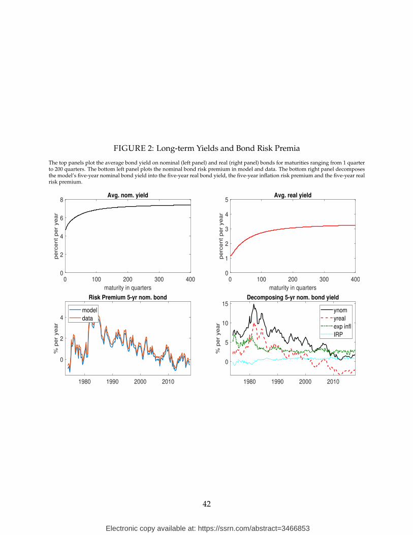
The top panels of Figure 2 show the model’s implications for the average nominal (left

panel) and real (right panel) yield curves at longer maturities. These long-term yields are

well behaved. The bottom left panel shows that the model matches the dynamics of the

nominal bond risk premium, defined as the expected excess return on five-year nominal

bonds. The compensation for interest rate risk varies substantially over time, both in data

and in the model. The bottom right panel shows a decomposition of the yield on a five-

year nominal bond into the five-year real bond yield, annual expected inflation over the

next five years, and the five-year inflation risk premium. On average, the 5.7% five-year

nominal bond yield is comprised of a 1.7% real yield, a 3.3% expected inflation rate, and

a 0.8% inflation risk premium. The importance of these components fluctuates over time.

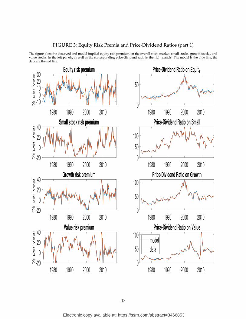
Figures 3 and 4 show the equity risk premium, the expected excess return, in the left

panels and the price-dividend ratio in the right panels. The various rows cover the seven

stock indices we price. The dynamics of the risk premia in the data are dictated by the

VAR. The model chooses the market prices of risk to fit these risk premium dynamics as

21


closely as possible.8 The price-dividend ratios in the model are formed from the price-

dividend ratios on the strips of maturities ranging from 1 to 3500 quarters, as explained

above. The figure shows an excellent fit for price-dividend levels and a good fit for risk

premium dynamics. Some of the VAR-implied risk premia have outliers which the model

does not fully capture. This is in part because the good deal bounds restrict the SDF from

becoming too volatile and extreme. We note large level differences in valuation ratios

across the various stock factors, as well as big differences in the dynamics of risk premia

and price levels, which the model is able to capture well.

3.3 Temporal Pricing of Risk

The first key input from the model into the private equity valuation exercise are the prices

of nominal zero-coupon bonds and of the various dividend strips. Figure 5 plots these

strip prices, scaled by the current quarter dividend. For readability, we plot only three

maturities: one, five, and ten years. The model implies substantial variation in strip prices

over time, across maturities, as well as across risky assets. If the replicating portfolio for

VC funds originated in the year 2000 loads heavily on growth strips, when growth strips

are expensive, then the risk-adjusted performance of vintage-2000 VC funds will be high,

all else equal.

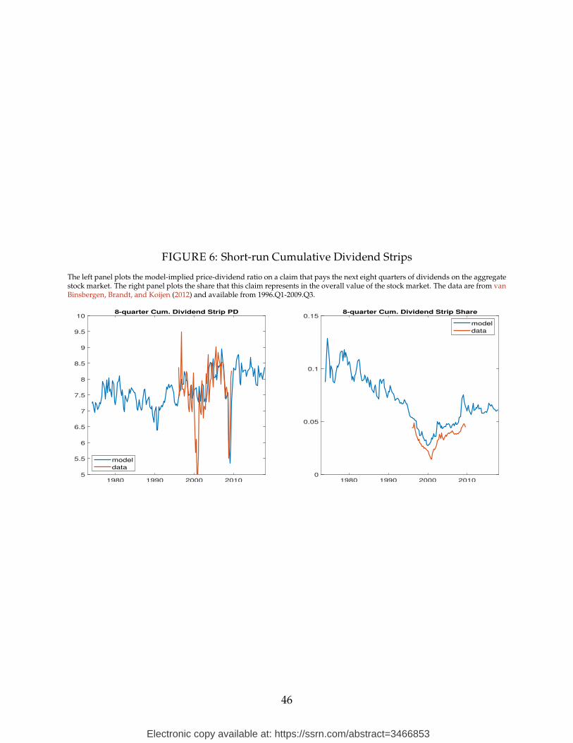
As part of the estimation, the model fits several features of traded dividend strips

on the aggregate stock market. Figure 6 shows the observed time series of the price-

dividend ratio on a claim to the first 8 quarters of dividends (red line, left panel), as well

as the share of the total stock market value that these first eight quarters of dividends

represent (red line, right panel). The blue line is the model. The model generates the right

level for the price-dividend ratio for the short-horizon claim. For the same 55 quarters

for which the data are available, the average is 7.75 in the model and 7.65 in the data.

The first 8 quarters of dividends represent 3.4% of the overall stock market value in the

data and 4.5% in the model, over the period in which there are data. The model mimics

the observed dynamics of the short-horizon value share quite well, including the sharp

decline in 2000.Q4-2001.Q1 when the short-term strip value falls by more than the overall

stock market. This reflects the market’s perception that the recession would be short-

lived. In contrast, the share of short-term strips increases in the Great Recession, both in

8The quarterly risk premia are annualized (multiplied by 4) for presentational purposes only. The VARdoes not restrict risk premia to remain positive. The VAR-implied market equity risk premium is negativein 21% of the quarters.

22


the data and in the model, in recognition of the persistent nature of the crisis.

The second key input from the model into the private equity valuation exercise are the

expected excess return on the bond and stock strips of horizons of 1-60 quarters. After all,

the expected return of the PE fund is a linear combination of these expected returns; re-

call equation (2). Figure 7 plots the average risk premium on nominal zero coupon bond

yields (top left panel) and on all dividend strips (other panels). Risk premia on nomi-

nal bonds are increasing with maturity from 0 to 3.5%. The second panel shows the risk

premia on dividend strips on the overall stock market (solid blue line). It also plots the

dividend futures risk premium (red line). The difference between the spot and futures

risk premium is approximately equal to the nominal bond risk premium. The uncondi-

tional dividend futures risk premium is downward sloping in maturity at the short end of

the curve, and then flattens out. The graph also plots the model-implied dividend futures

risk premium, averaged over the period 2003.Q1-2014.Q2 (yellow line). It is substantially

more downward sloping at the short end than the risk premium averaged over the entire

1974-2017 sample. In fact, the model matches the realized portfolio return on dividend fu-

tures of maturities 1-7 years over the period 2003.Q1-2014.Q2, which is 8.7% in the data

and 8.7% in the model.9

The remaining panels of Figure 7 show the dividend strip risk spot and future pre-

mia for the other cross-sectional factors. There are interesting differences in the levels of

future risk premia especially at shorter horizons and in the shape of term structures. Av-

erage futures risk premia are generally declining to flat in maturity. Heterogeneity in risk

premia by asset class, by horizon, and over time will give rise to heterogeneity in the risk

premia on the PE-replicating portfolios.

Figure 8 plots the time series of expected returns on bonds and on both dividend and

gain strips for the seven equity factors; the maturity of all strips is 20 quarters. Expected

returns are annualized. We note rich cross-sectional heterogeneity in levels and dynamics

across panels, a low-frequency decline over time in the level of expected returns common

across most panels, and high pairwise correlation between dividend and capital gain strip

expected returns in each panel.

Appendix C provides further insight into how the model prices risk at each horizon

using tools developed by Hansen and Scheinkman (2009) and Borovicka and Hansen

(2014). The shock price elasticities measure how the model prices risk exposure to each

9As an aside, the conditional risk premium, which is the expected return on the dividend futures portfolioover the 2003.Q1-2014.Q2 period is 6.0% per year in the model. The unconditional risk premium on thedividend futures portfolio (over the full sample) is 5.2%.

23


VAR innovation at various horizons. The shock exposure elasticities measure how cash

flow (dividend) growth on each of the seven listed equity factors responds to an impulse

in inflation, GDP growth, short rates, the slope of the term structure, and shocks to the

cash flows themselves. It makes clear that the various equity factors have very different

risk exposures from each other, and at various horizons.

4 Expected Returns and Risk-adjusted Profits in PE Funds

In this section, we combine the cash-flow exposures from section 2 with the asset prices

from section 3 to obtain risk-adjusted profits on private equity funds.

4.1 Summary Statistics

Our fund data cover the period January 1981 until December 2017. Our main data source

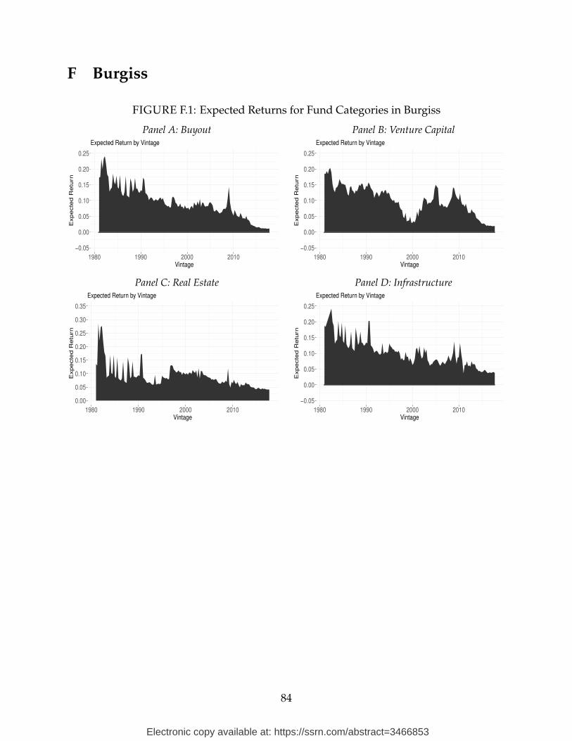
is Preqin, but we also replicate our analysis using data from Burgiss in Appendix F.10 We

group private equity funds into eight categories: Buyout (LBO), Venture Capital (VC),

Real Estate (RE), Infrastructure (IN), Natural Resources (NR), Fund of Funds (FF), Debt

Funds (DF), and Restructuring (RS). Our FF category contains the Preqin categories Fund

of Funds, Hybrid Equity, and Secondaries. The Buyout category is commonly referred to

as Private Equity, whereas we use the PE label to refer to the combination of all investment

categories.

We include all funds with non-missing cash-flow information. We group funds by

their vintage, defined as the quarter in which they make their first capital call. The last

vintage we consider in the analysis is 2017.Q4. Table 1 reports the number of funds and

the aggregate AUM in each vintage-category pair. In total, we have 4,219 funds in our

analysis and an aggregate of $4.1 trillion in assets under management. There is clear

business cycle variation in when funds funds get started as well as in their size (AUM).

Buyout is the largest category by AUM, followed by Real Estate, and then Venture Cap-

ital. The last column of the table shows the quartile of the price/dividend ratio on the

stock market, which we use to estimate vintage effects. The table reports the average

pd-quartile across of the four vintages (quarters) in the calendar year.

10One possible limitation of the Preqin data is it is substantially sourced by FOIA requests made to pub-lic pensions, who may have differential pricing terms in side letters and “Most Favored Nation” clauses.However, Da Rin and Phalippou (2017) suggests that public pensions are not statistically different fromother investors in their access to these clauses. Burgiss data is sourced instead from a more representativeset of institutional investors.

24


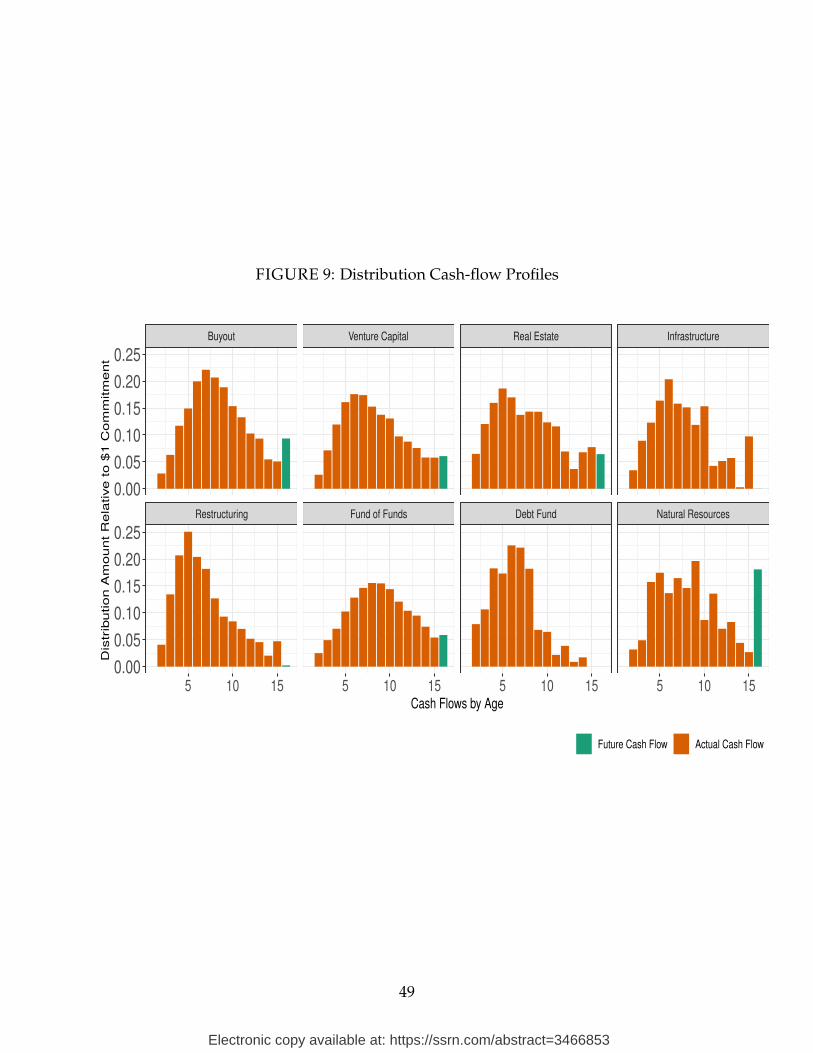
Figure 9 shows the average cash-flow profile in each category for distribution events,

pooling all funds and vintages together and equally weighting them. For this graph, we

combine all monthly cash-flows into one yearly cash-flow for each fund, and then average

across funds within the category. The first 15 orange bars are for the first 15 years since the

first capital call. The last bar (in green) represents the discounted sum of cash flows that

occur after year 15.11 The literature often treats PE vehicles as lasting for about ten years.

While we observe that the majority of distribution cash-flows occur between years 5 and

10, cash flows after year 10 account for a substantial portion of the total cash received by

LPs, and we therefore incorporate them in our analysis.12 All cash flows are net of fees

imposed by the GPs.

Figure 10 zooms in on the four investment categories of most interest to us: LBO, VC,

RE, and IN. The figure shows the average cash-flow profile for each vintage. Since there

are few LBO and VC funds prior to 1990 and few RE and IN funds prior to 2000, we start

the former two panels with vintage year 1990 and the latter two panels with vintage year

2000. The figure shows that there is substantial variation in cash-flows across vintages,

even within the same investment category. This variation will allow us to identify vintage

effects. The figure also highlights that there is a lot of variation in cash-flows across calen-

dar years. VC funds started in the mid- to late-1990s vintages realized very high average

cash-flows around calendar year 2000 and a sharp drop thereafter. Since the stock market

also had very high cash-flow realizations in the year 2000 and a sharp drop thereafter, this

type of variation will help the model identify a high stock market beta for VC funds. This

is an important distinction with other methods, such as the PME, which assume constant

risk exposure and so would attribute high cash flow distributions in this period to excess

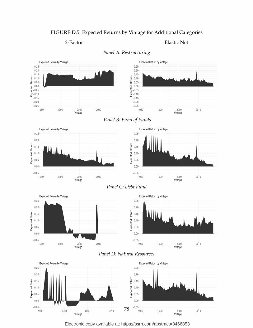
returns. Appendix Figure D.1 shows cash-flow profiles for the remaining fund categories.

11We discount at the risk free rate produced by the Asset Pricing model. For infrastructure, we have afew outliers in years 14 and 15. To avoid overfitting in the OLS model, we discount these cash flows (butdo not discard them) to the thirteenth year, which improves ease of interpretability but does not affect ourconclusion.

12Industry publications have also noted the increasing lifespan of private equity funds. For instance, aPreqin report from 2016 remarks: “The average lifespan of funds across the whole private capital industryis increasing beyond the typical 10 years... older funds of vintages 2000-2005 still hold a substantial $204bnworth of investments, equating to 7.2% of total unrealized assets” (Preqin, 2016). We also estimate ourresults on a subsample of funds which only distribute 10% or less of their cash after 10 years, and findcomparable results.

25


4.2 Factor Estimation in OLS and Elastic Net

We compare the results of two estimation approaches, run separately for each fund cate-

gory. The first is a two-factor model (bond and aggregate stock dividend strips) estimated

by OLS; recall equation (6). The second is an Elastic Net model estimated on the full set

of fifteen factors (bonds strips, and dividend and capital gains strips for: aggregate stock

index, small stocks, growth stocks, value stocks, REITs, infrastructure stocks, and natu-

ral resource stocks); recall equations (7) and (8). The estimated parameters are the factor

exposures across horizon, bkh, and how these exposures shift by vintage (pd quartile), cap-

tured by the akt . Their sum, ak

t + bkh, measures the number of units of factor strip k with

maturity h that the PE-replicating portfolio buys.

This Elastic Net approach has the main benefit that it results in substantial dimension

reduction of our estimation problem (through its two regularization terms), which is es-

sential in estimating a large number of parameters across a variety of horizons, factors,

and vintage states. Absent this dimensionality reduction, we simply would be unable

to estimate an asset pricing model with a rich set of possible factors given the limited

number of PE fund observations. The end result is a parsimonious replicating portfolio

consisting of long positions in a modest number of strips (factor-horizon combinations).

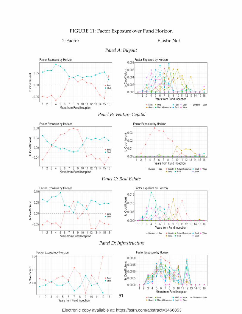
Figure 11 contrasts our resulting factor exposures along the dimension of horizon bh

obtained through both the 2-factor OLS model (left) and the Elastic Net model using the

full set of factors (right). Each row corresponds to one of the four main PE categories.

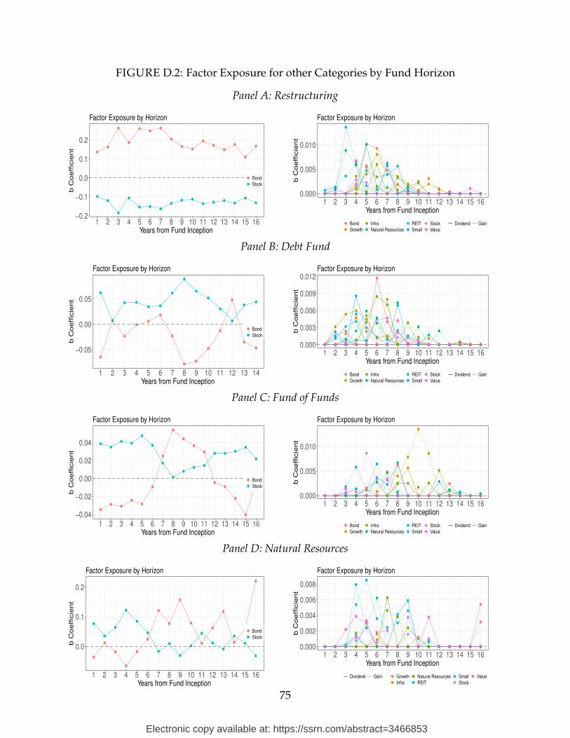
Appendix Figure D.2 contains these estimates for the other four PE categories. Appendix

Figures D.3 and D.4 contain these estimates for the PD-quartile effects at.

Buyout In Panel A of Figure 11 , we find substantial stock exposures throughout most

of the life of the fund. The replicating portfolio contains short positions in bonds, excep-

tion for the middle years (7-12) and the terminal cash flow represented by year 16. This

terminal cash exposure is captured by a mix of stock and bond strips.

The Elastic Net model on the right differs in several respects. First, all positions are

positive, which ensures that PE cash flows are replicable through long-only positions.

Second, the two factors in the OLS model for find little weight in the Elastic Net model.

This suggests that other cross-sectional factors better capture the systematic risk in Buy-

out funds. The regularization in the Elastic Net approach ensures sufficient dimension

reduction in order to produce a sparse portfolio of replicating positions. We uncover a

pattern of dividend strip (solid lines) and capital gain strip (dotted lines) exposures that

26


is rich and complex. While we have not constrained our estimation to require that ad-

jacent years have similar exposures, we frequently find that factors have some periodic

tendencies with rising and falling exposures over the fund’s life cycle.

Early on in fund life, PE fund cash flows tend to look more like aggregate stocks,

value stocks, and small stocks. Closer to to the end of the fund life, we estimate a much

more substantial growth exposure. This suggests that the early cash flows, when portfolio

companies have been purchased and are either quickly re-sold or harvested for operating

profits, have exposures which look like small, value, and general stock market. By the

end of the fund life, the exposure looks closer to the capital realization of growth stocks.

This overall pattern generally corresponds to Buyout fund activities which consist of pur-

chasing a broad range of companies, restructuring the operations, harvesting some initial

cash flows (for instance through dividend recapitalization), and ultimately reselling these

assets on public markets. We also find some moderate evidence for non-standard divi-

dend cash flows (such as from REITs around year 8, and infrastructure in years 9-11 of

fund life). To minimize over-fitting, we rely on a cross-validation exercise in which we

use a leave-out sample to fit λ1 and λ2 parameters.

The takeaway from the analysis on Buyout funds is that these vehicles do not simply

take on bond and equity exposure in the cross-section, as is commonly assumed. Our

best estimate for fund cash flow fit features a much richer factor exposure structure across

different equity factor categories and horizons. This factor exposure is relevant for LPs

who invest in Buyout vehicles. Portfolio management of PE within institutional investor

portfolios should take into account the rich risk and return dynamics of PE funds.

Venture Capital We see further evidence of the importance of considering a broad cross-

section of factor exposures in Panel B of Figure 11 , which examines Venture Capital funds.

Our OLS 2-factor model in the left panel places some positive weight on the equity div-

idend factor both early and late in fund life, but finds that a bond position best fits cash

distributions for the most active middle part of the funds’ life.

Instead, our Elastic Net model (right panel) indicates that the single factor which con-

tributes most to the fit of VC cash flows for the first nine years of fund life is gains strips

on growth stocks. VC cash flows are akin to the cash flows obtained from selling firms

in the bottom quintile of the book-to-market distribution. Appendix Figure D.3 suggests

that this loading is even higher in periods when the market has a higher pd ratio.

Our findings for VC funds carry an important economic intuition. While Buyout funds

27


acquire a range of companies which may differ in their underlying factor exposures; VC

funds concentrate on early-stage and rapidly expanding entrepreneurial companies and

distribute little cash prior to their exits from these funds. Further VC funds, unlike Buyout

(or Real Estate, or Infrastructure funds) typically harvest few cash flows during fund

operations prior to deal exits. Correspondingly, we find that the bulk of VC fund cash

flow exposure can be accounted for by growth gains strips.

Real Estate Panel C repeats our estimation for Real Estate funds. Stock dividend strips

have a positive loading throughout fund horizon in the OLS model. Bond positions are

negative except for some of the middle years. Again, our Elastic Net model picks up ad-

ditional cross-sectional exposures which crowd out the exposure to aggregate stock and

bond market strips from the two-factor model. Reassuringly, REIT dividends and REIT

gains strips are important components of the replicating portfolio. The early cash flow

distributions also load on value and small stock gain strips. In the later years, REPE fund

cash flows are exposed to the same risk as infrastructure dividends strips and growth

gains strips. These results suggest that Real Estate funds take on a distinct factor expo-

sure profile from Buyout and VC funds, while sharing at least some of the same factor

exposures.

Infrastructure Panel D studies Infrastructure funds. Here, too, we find a strong role

for sector-specific factors, such as infrastructure dividend strips, natural resource gains

strips, and REIT gains strips which point to the role of underlying asset characteristics

in driving the fund-level asset pricing profile.13 Interestingly, the infrastructure category

tends to place greater weight on dividend strips, as opposed to capital gains strips; sug-

gesting that the cash flows in this sector are more like dividends than like realized prices.

Take-aways These rich dynamics across horizon, price-to-dividend ratios, and factors

have important asset pricing implications. The risk loadings on PE funds broadly cannot

be assumed to be static either in the time-series or across fund age (maturity). Rather, a

broad set of risk factor exposures is relevant across all PE fund categories. We provide

the first systematic analysis of the asset pricing properties of these some of these alterna-

tive fund categories (RE, IN, NR), and find that they carry important sector-specific asset

exposures. These exposures are frequently concentrated in the first half of the fund’s

13Similarly, Natural Resource funds, which we examine in the Appendix, have greater natural resourcestrip exposure.

28


life. Our estimation approach allows us to translate these complex risk dynamics into the

expected return for different fund categories and to revisit the question of performance

evaluation. We turn to expected returns next.

4.3 Expected Return

With the replicating portfolio of zero-coupon bonds and dividend strips in hand (expres-

sions are detailed in Appendix A), we can calculate the expected return on PE funds

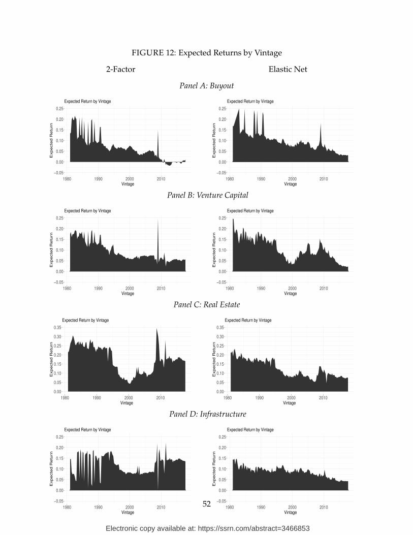
in each investment category using equation (2). Figure 12 plots the time-series of the

expected return for the four main PE categories. It aggregates over all of the different

horizon effects and annualizes the resulting expected return as per equation (4). The left

panels of this figure are for the 2-factor OLS model; the right panels for the Elastic Net

model with 15 factors. Appendix Figure D.5 reports the results for other 4 PE categories.

Generally, the Elastic Net delivers expected returns that look more reasonable in levels

and dynamics than the two-factor OLS model.

Time variation in the factor exposures coming through dependence on the pd-quartile

of the vintage combines with time variation in expected returns on dividend and gain

strips driven by the state variables of the VAR to generate time variation in the expected

return on PE funds. The annualized expected returns that investors can anticipate on

their PE investments as compensation for systematic risk has seen large variation over

time, with a declining pattern at low frequencies. The low-frequency decline is inherited

from a low-frequency decline in strip expected returns; recall Figure 8.

At higher frequencies we note the low expected return around the year 2000, when the

stock market peaked, and an increase in risk premia during the Great Recession. Since

then, expected returns have lowered substantially, especially for Buyout, VC, and Infras-

tructure. In the RE category, we observe higher expected returns since the Great Recession

than in the other categories.

4.4 Performance Evaluation

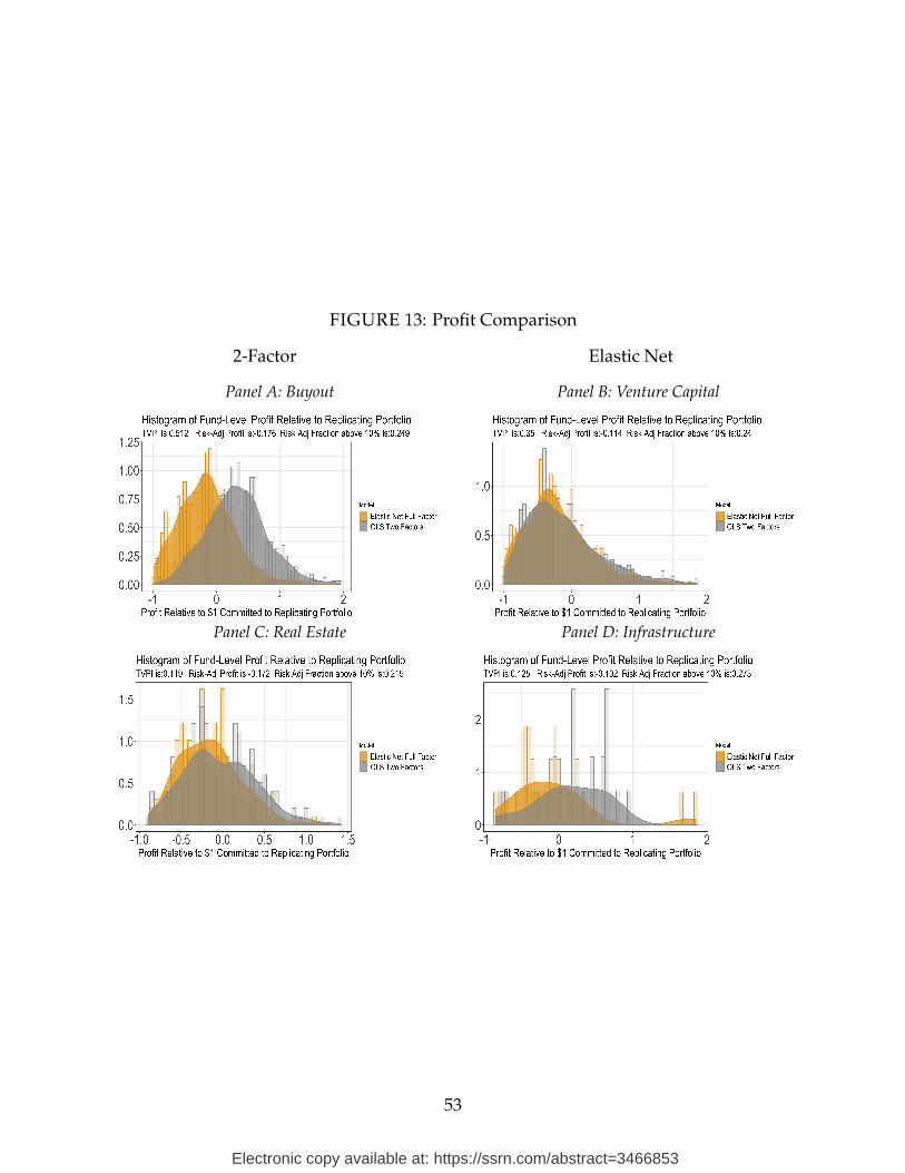
Next, we turn to performance evaluation. Figure 13 plots the histogram of Risk-Adjusted

Profits (RAP) for the two-factor OLS (gray) and 15-factor Elastic Net (yellow) models

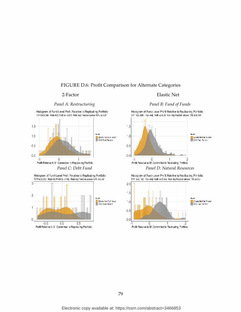
for Buyout, VC, RE, and IN. The four alternate PE categories are shown in Figure D.6.

Recall from equation (5) that the RAP for each fund compares the realized cash flow

distributions against the realized payoffs from the replicating portfolio, as well as the

29


difference in the purchase price of the replicating portfolio and the $1 commitment in the

PE fund. A kernel density is estimated from the discrete histogram.

In Buyout, RE, and IN, the entire profit distribution is shifted to the left under the

Elastic Net model. PE funds are less profitable on a risk-adjusted basis once we account

for a richer cross-section of factor exposures through our Elastic Net model. As a result,

an LP using traditional approaches (TVPI) and even a flexible two-factor model would

attribute a fund’s performance to outperformance, which the Elastic Net model would

instead attribute much of the profit as compensation for risk.

This reduction in apparent outperformance is strongest in the Buyout category. While

the risk-adjusted profits are positive under the two-factor model, they are negative on

average in our benchmark Elastic Net model, at -21 cents per dollar invested. This average

RAP masks substantial cross-sectional dispersion. Around a quarter of funds outperform

by at least 10% in the full model. We find a similar pattern in VC: the average RAP for

VC funds with our full elastic net model is is -11 center per dollar invested; also about a

quarter of VC funds generate greater than 10 cents in RAP.

The results for RE look similar to those for Buyout. The extra risk exposure shifts the

RAP distribution to the left. Average RAP is -17 cents and 22% of funds have a RAP

greater than 10%. The average IN fund fares slightly better with an average RAP of -10

cents and 27% of funds generating more than 10 cents in risk-adjusted profit.

Figure 14 plots the average RAP by vintage for both the OLS (left) and Elastic Net

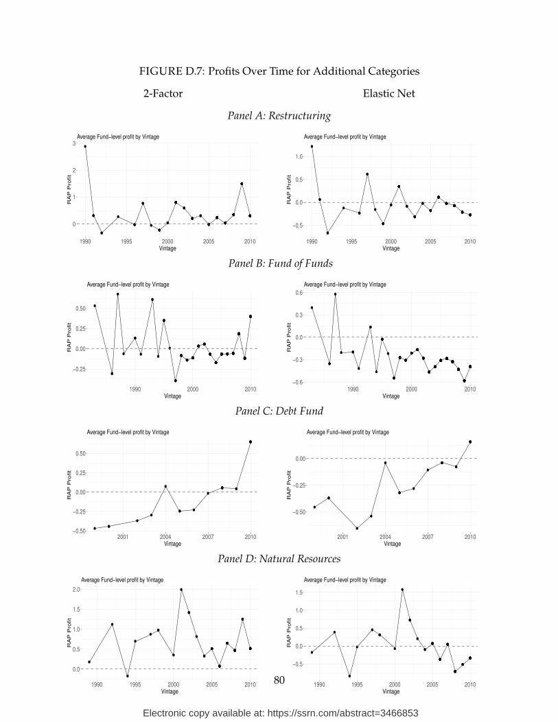
(right) models. Appendix Figure D.7 plots these estimates for alternate fund categories.

While the general time-series for profits are similar across both sets of models, there are

also notable differences. For instance, in the Buyout category, we observe positive profits

continuing through the most recent vintages in the OLS model. By contrast, our Elas-

tic Net model estimates positive profits for a few historic vintages, but largely negative

average profits for vintages since 1995.

While we observe extremely high profits for VC funds originated in the mid-1990s,

these profits fall by a factor of two in the Elastic Net model. Recent VC vintages have

generated negative RAPs. Real estate funds started just before the Great Recession (2004-

2006) have performed very poorly, losing 30 cents on a risk-adjusted basis. The last vin-

tage we consider in this graph (2010) is faring much better.

30


4.5 Model Comparison

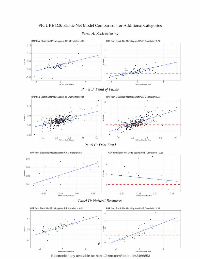
It is instructive to benchmark our results across other approaches pursued in the litera-

ture. Figure 15 graphically compares the results from the Elastic Net model for our main

PE categories against two commonly used PE fund performance metrics: IRR and PME.

Appendix Figure D.8 repeats the analysis for the additional categories. The left panels

plot fund-level IRR against our fund-level RAP measure; the right panels plot fund-level

PME against fund-level RAP. The key takeaway from this comparison is a similar rank-

ing of fund performance. Our measure of RAP generally correlates between 70% and 90%

with the IRR and PME measures in the cross-section of funds. The correlation is higher

with the PME than with the IRR measure in the Buyout and VC categories for which we

have the most data. This is reasonable as the PME approach also incorporates a role for

public market assets. The similarity lends credibility to our measure of RAP. The mea-

sures are not identical, however, so that there are funds which conventional measures

assess to be high-performing but our estimates suggest only offer fair (or even too little)

compensation for factor risk exposure.

Table 2 compares average outperformance. Panel A shows results from Preqin, our

primary data source. We repeat our analysis on the Burgiss data set, which has broader

coverage of 7,193 PE funds, in Panel B. We show complete results from Burgiss in Ap-

pendix F. We discuss the Preqin results first. The first three rows of Panel A reflect stan-

dard measures to evaluate PE funds: the TVPI, IRR, and PME. The next two rows display

our two-factor OLS and 15-factor Elastic Net models. The columns report the R2 from the

factor model estimation, the average RAP, and the cross-sectional standard deviation of

the RAP. We focus on the four main fund categories.

For Buyout funds, the two-factor Elastic Net model has an R2 of 0.156, and an average

risk-adjusted profit of 29 cents per dollar invested. Relative to the average PME of 36

cents, the lower RAP estimate reflects the refined equity exposure estimate, compared

with the PME which assumes that all funds have an equity beta of one.

Next, we add additional factors and estimate the impact on model fit and RAP. For

Buyout, the model fit of the Elastic Net improves to 0.160. In addition to the improve-

ment in model fit, we observe substantially different profit estimates. The average RAP

for the Buyout category is -17.6 cents for the Elastic Net model compared with 29.1 for

the two-factor model. Under the richer model of systematic risk, we obtain a lower es-

timate of risk-adjusted outperformance. In other words, while the cash flow estimation

improves modestly when adding more equity factors, the systematic risk exposure of the

31


PE funds can now be replicated more cheaply and so results in a substantially lower esti-

mate of PE fund profit. The Elastic Net model also results in a tighter distribution (lower

cross-sectional standard deviation) of RAP. The last row reports the results for a model

where the cash flows of all funds in a particular fund category-vintage pair are aggre-

gated, and then an Elastic Net model is estimated on the aggregate cash flows. It gener-

ally shows higher R2, suggesting that there is substantial idiosyncratic risk in individual

fund returns (just like there is in individual stocks). The average RAP estimates obtained

on aggregated fund cash flows are similar. To better assess the role of idiosyncratic risk;

in Appendix E we perform our analysis on public equities. We find similarly moderate R2

when we fit dividend strips against individual stocks; but substantially higher R2 when

we fit our model on portfolios.

The message for the other fund categories is similar. Richer risk adjustment results is

much lower average RAPs and a tighter distribution. The full-factor Elastic Net results in

an average RAP that is 23 cents lower than that predicted by the two-factor OLS model

for VC funds, 14 cents lower for RE funds, and 39 cents for IN funds. We also note the

much wider cross-sectional dispersion in VC fund performance compared to the other PE

categories.

Next, we examine the persistence of the various performance metrics, defined as the

correlation between profits across the different measures between adjacent funds from the

same PE firm. We use fund vintages to examine the autocorrelation of returns between the

current fund and the immediately preceding fund in the sequence. In the first three rows

of Panel A, we report persistence for the traditional performance metrics such as TVPI,

IRR, and PME. Consistent with prior research (Harris, Jenkinson, Kaplan, and Stucke,

2014), we find substantial persistence in performance across funds originated within the

same firm across time. However, we tend to observe less persistence when we include

additional factor controls. For example, the persistence of PME for VC funds is 0.43 while

the persistence according to the Elastic Net model is only 0.15. Similarly, the persistence

of REPE funds falls from 0.40 to 0.20. This result sheds new light on the puzzle of ex-

cess persistence in PE fund outperformance. A portion of this persistence is due to some

firms specializing in strategies that have a common risk factor exposure across the funds

under their management. Accounting for this factor exposure lowers the measure of per-

sistence.14

14We also examine the persistence of factor exposure across funds within the same firm family and findpersistence in factor exposures estimated on the first fund started by firms, and subsequent funds estimatedthrough separate regressions. This also suggests our factor exposure measure results in a robust measure

32


Panel B of Table 2 repeats the analysis on the Burgiss data which has more expan-

sive coverage in general, but especially in the VC and infrastructure categories. Examin-

ing this data set allows us to address possible sample selection issues in the Preqin data

set. Reassuringly, we find very similar results across the two data sets. In particular,

we find that average RAPs are generally estimated to be negative using our full-factor

approach. The model fit for aggregated cash flows (last row) tends to be higher in the

Burgiss than in the Preqin data. In the VC category, Burgiss has better coverage of certain

high-performing funds which do not report to Preqin. Indeed, we find that average TVPI

if 53 cents in Burgiss and 35 cents in Preqin. However, we continue to find negative es-

timates of risk-adjusted profits for VC: -7.4 cents in Burgiss versus -11.4 cents in Preqin.

Similarly, the better coverage of infrastructure PE funds does not overturn the finding of

negative average RAP. In fact the average RAP from the Elastic Net model is -21 cents in

Burgiss compared to -10 cents in Preqin.

Our pervasive finding of negative average RAP stands in contrast to previous lit-

erature in private equity which has generally found evidence of fund outperformance

(Brown, Harris, Jenkinson, Kaplan, and Robinson, 2015; Kaplan and Sensoy, 2015; Harris,

Jenkinson, and Kaplan, 2014). The difference is made apparent when comparing standard

performance metrics in the first three rows, which tend to show more favorable perfor-

mance statistics. Even the two-factor model generally shows positive profits. Our more

negative conclusion about excess returns in the private equity industry is a natural conse-

quence of risk-adjustment due to cross-sectional factor exposure. Similar risk adjustments

in the mutual fund (Fama and French, 2010) or hedge fund space (Fung, Hsieh, Naik, and

Ramadorai, 2008) tend to substantially lower outperformance. We find the same is true

for private equity funds, a point that has surprisingly not been made before. We also

find evidence for substantial cross-sectional dispersion in RAPs, as well as sizable persis-

tence in risk-adjusted performance over time. This suggests that there may be a subset of

PE managers that consistently delivers outsized returns. This finding is consistent with

Kacperczyk, Van Nieuwerburgh, and Veldkamp (2014, 2016) who find that a small right

tail of mutual fund managers consistently outperforms, although the earlier mutual fund

literature has been skeptical of skill in any part of the fund distribution (Fama and French,

2010).

Similar findings of limited excess returns across different categories of delegated asset

managers are suggestive of similar economic forces at work. First, investors may find it

of fund risk attributes.

33


difficult to replicate complex factor strategies on their own, and so may be willing to pay

managers to generate factor strategies. Second, superior performance tends to be associ-

ated with higher fund flows, leading to increased capital commitments which diminish

returns in the presence of decreasing returns to scale, along the lines of Berk and Green

(2004). As the PE industry has grown substantially, there may be insufficient economies of

scale to adequately manage a growing asset base to generate the same outsize returns of

previous periods. Finally, delegated asset managers charge sizable management and per-

formance fees especially when financial products are more opaque and complex (Celerier

and Vallee, 2015) as they are in PE. This lowers post-fee returns for investors further.

5 Conclusion

We provide a novel valuation method for private equity cash-flows that decomposes the

cash-flow at each horizon into a systematic component that reflects exposure to various

sources of aggregate risk, priced in listed securities markets, and an idiosyncratic compo-

nent which reflects the risk-adjusted profit to the PE investor. The systematic component

represents a portfolio of stock and bond strips paying safe or risky cash flows at horizons

over which PE funds make cash flow distributions. A state-of-the-art no-arbitrage asset

pricing model estimates prices and expected returns for these strips, fitting the time series

of bond yields and stock prices, including dividend strips. It provides the first estimates

of the term structure of risk and return in the cross-section of equity factors.

Using both OLS and Elastic Net approaches, we estimate rich heterogeneity in PE

fund risk exposures across horizons, in the cross-section, and in the time-series. PE funds’

risk exposure is best modeled not only using bonds and the aggregate stock market, but

is improved with the addition of sector-specific equity factor exposures. The estimated

exposures are sensible given the nature of underlying nature of PE assets, and indicate an

important role for growth and small stocks in Venture Capital and for REITs in real estate

funds. In the time series, we find that expected returns on PE funds have been declining

substantially since the 1980s and especially since the Great Recession, reflecting declining

risk premia in public markets.

On average, PE funds considerably underperform their replicating portfolio bench-

mark, suggesting that while PE funds offer investors access to complex risk exposures,

they do so at a more expensive price than offered in public markets. While our resulting

profit measures correlate well with existing measures of outperformance in the cross-

34


section of funds, they suggest both lower average performance and less performance per-

sistence.

Our analysis highlights the value of a methodological advance in the assessment of

risk and return for unlisted assets, which are an increasing component of the total in-

vestable universe for many institutional investors. While Private Equity is an especially

important application of our approach, given its size, our method can be applied more

broadly to study the asset pricing characteristics of any other cash-flowing asset that is not

listed on the capital markets. Individual real estate or infrastructure investment projects

are a key application left for future work.

35


References

Ammar, S. B., and M. Eling, 2015, “Common risk factors of infrastructure investments,”

Energy Economics.

Andonov, A., R. Kraussl, and J. Rauh, 2018, “The Subsidy to Infrastructure as an Asset

Class,” Working Paper 25045, National Bureau of Economic Research.

Ang, A., B. Chen, W. N. Goetzmann, and L. Phalippou, 2017, “Estimating Private Equity

Returns from Limited Partner Cash Flows,” Netspar Discussion Paper No. 06/2014-021;

Said Business School WP 2014-8.

Ang, A., and M. Piazzesi, 2003, “A No-Arbitrage Vector Autoregression of Term Structure

Dynamics with Macroeconomic and Latent Variables,” Journal of Monetary Economics,

50, 745–787.

Berk, J. B., and R. C. Green, 2004, “Mutual Fund Flows and Performance in Rational

Markets,” Journal of Political Economy, 112(6), 1269–1295.

Bokberg, A., J. Carrellas, A. Chau, and C. Duane, 2019, “Private markets come of age

McKinsey Global Private Markets Review,” working paper, McKinsey Global Institute.

Borovicka, J., and L. P. Hansen, 2014, “Examining Macroeconomic Models through the

Lens of Asset Pricing,” Journal of Econometrics, 183(1), 67–90.

Brown, G., R. Harris, T. Jenkinson, S. N. Kaplan, and D. Robinson, 2015, “What Do Differ-

ent Commercial Data Sets tell Us About Private Equity Performance?,” Working Paper

University of North Carolina Kenan Institute.

Campbell, J. Y., 1991, “A Variance Decomposition for Stock Returns,” Economic Journal,

101, 157–179.

, 1993, “Intertemporal Asset Pricing Without Consumption Data,” American Eco-

nomic Review, 83(3), 487–511.

, 1996, “Understanding Risk and Return,” The Journal of Political Economy, 104(2),

298–345.

Campbell, J. Y., and R. J. Shiller, 1991, “Yield Spreads and Interest Rate Movements: A

Bird’s Eye View,” Review of Economic Studies, 58, 495–514.

36


Celerier, C. M., and B. Vallee, 2015, “The Motives for Financial Complexity: An Empirical

Investigation,” SSRN, (2289890).

Cochrane, J. H., 2005, “The risk and return of venture capital,” Journal of Financial Eco-

nomics, 75, 3–52.

Cochrane, J. H., and M. Piazzesi, 2006, “Decomposing the Yield Curve,” Working Paper,

University of Chicago.

Cochrane, J. H., and J. Saa-Requejo, 2000, “Beyond Arbitrage: ’Good deal’ asset price

bounds in incomplete markets,” Journal of Political Economy, 108, 79–119.

Cox, J., J. Ingersoll, and S. Ross, 1985, “An Intertemporal General Equilibrium Model of

Asset Pricing,” Econometrica, 53, 363–384.

Da Rin, M., and L. Phalippou, 2017, “The importance of size in private equity: Evidence

from a survey of limited partners,” Journal of Financial Intermediation, 31, 64–76.

Dai, Q., and K. J. Singleton, 2000, “Specification Analysis of Affine Term Structure Mod-

els,” Journal of Finance, 55, 1943–1978.

Driessen, J., T.-C. Lin, and L. Phalippou, 2012, “A new method to estimate risk and re-

turn of nontraded assets from cash flows: The case of private equity funds,” Journal of

Financial and Quantitative Analysis, 47(3), 511–535.

Duffie, D., and R. Kan, 1996, “A Yield Factor Model of Interest Rates,” Mathematical Fi-

nance, 6, 379–406.

Ewens, M., C. M. Jones, and M. Rhodes-Kropf, 2013, “The Price of Diversifiable Risk in

Venture Capital and Private Equity,” Review of Financial Studies, 26, 1854–1889.

Fama, E. F., and K. R. French, 1992, “The Cross-Section of Expected Stock Returns,” The

Journal of Finance, 47(2), 427–465.

, 2010, “Luck versus Skill in the Cross-section of Mutual Fund Returns,” The Journal

of Finance, 65(5), 1915–1947.

Fung, W., D. A. Hsieh, N. Y. Naik, and T. Ramadorai, 2008, “Hedge Funds: Performance,

Risk, and Capital formation,” The Journal of Finance, 63(4), 1777–1803.

37


Gompers, P. A., and J. Lerner, 1997, “Risk and Reward in Private Equity Investments: The

Challenge of Performance Assessment,” Journal of Private Equity, 1, 5–12.

Gu, S., B. Kelly, and D. Xiu, 2018, “Empirical Asset pricing via Machine Learning,” Na-

tional Bureau of Economic Research Working Paper No. 25398.

Haddad, V., E. Loualiche, and M. Plosser, 2017, “Buyout activity: The impact of aggregate

discount rates,” The Journal of Finance, 72(1), 371–414.

Hansen, L. P., and J. Scheinkman, 2009, “Long-Term Risk: An Operator Approach,” Econo-

metrica, 77 (1), 177–234.

Harris, R. S., T. Jenkinson, and S. N. Kaplan, 2014, “Private Equity Performance: What Do

We Know?,” Journal of Finance, 69(5).

Harris, R. S., T. Jenkinson, S. N. Kaplan, and R. Stucke, 2014, “Has Persistence Persisted

in Private Equity? Evidence from Buyout and Venture Capital Funds,” .

Kacperczyk, M., S. Van Nieuwerburgh, and L. Veldkamp, 2014, “Time-Varying Fund

Manager Skill,” Journal of Finance, 69, 1455–1484.

, 2016, “Rational Attention Allocation over the Business Cycle,” Econometrica, 84,

571–626.

Kaplan, S., and B. Sensoy, 2015, “Private Equity Performance: A Survey,” Annual Review

of Financial Economics, 7, 597–614.

Kaplan, S. N., and A. Schoar, 2005, “Private equity performance: Returns, persistence,

and capital flows,” Journal of Finance, 60(4), 1791–1823.

Koijen, R. S. J., H. Lustig, and S. Van Nieuwerburgh, 2017, “The Cross-Section and Time-

Series of Stock and Bond Returns,” Journal of Monetary Economics, 88, 50–69.

Korteweg, A., and S. Nagel, 2016, “Risk-Adjusting the Returns to Venture Capital,” Jour-

nal of Finance, 71(3), 1437–1470.

Korteweg, A., and M. Sorensen, 2010, “Risk and return characteristics of venture capital-

backed entrepreneurial companies,” Review of Financial Studies, 23(10), 3738–3772.

, 2017, “Skill and Luck in Private Equity Performance,” Journal of Financial Eco-

nomics, 0.

38


Kozak, S., S. Nagel, and S. Santosh, 2017, “Shrinking the Cross Section,” National Bureau

of Economic Research Working Paper No. 24070.

Lettau, M., and J. Wachter, 2011, “The Term Structures of Equity and Interest Rates,”

Journal of Financial Economics, 101 (1), 90–113.

Ljungqvist, A., and M. Richardson, 2003, “The cash flow, return and risk characteristics

of private equity,” Working Paper, NYU Stern.

Lustig, H., S. Van Nieuwerburgh, and A. Verdelhan, 2013, “The Wealth-Consumption

Ratio,” Review of Asset Pricing Studies, 3(1), 38–94., Review of Asset Pricing Studies.

Metrick, A., and A. Yasuda, 2010, “The economics of private equity funds,” Review of

Financial Studies, 23(6), 2303–2341.

Peng, L., 2001, “Building a Venture Capital Index,” Working Paper.

, 2016, “The risk and return of commercial real estate: A property level analysis,”

Real Estate Economics, 44(3), 555–583.

Phalippou, L., and O. Gottschalg, 2009, “The performance of private equity funds,” Re-

view of Financial Studies, 22(4), 1747–1776.

Preqin, 2016, “The 2016 Preqin Global Private Equity and Venture Capital Report,” Preqin,

London, UK.

Robinson, D. T., and B. A. Sensoy, 2011, “Cyclicality, Performance Measurement, and

Cash Flow Liquidity in Private Equity,” Working Paper.

Sagi, J. S., 2017, “Asset-level risk and return in real estate investments,” Working Paper,

UNC Kenan-Flagler Business School.

Sorensen, M., and R. Jagannathan, 2015, “The Public Market Equivalent and Private Eq-

uity Performance,” Financial Analysts Journal, 71(4), 43–50.

Sorensen, M., N. Wang, and J. Yang, 2014, “Valuing private equity,” Review of Financial

Studies, 27(7), 1977–2021.

van Binsbergen, J., M. Brandt, and R. Koijen, 2012, “On the Timing and Pricing of Divi-

dends,” American Economic Review, 102(4), 1596–1618.

39


van Binsbergen, J. H., W. H. Hueskes, R. Koijen, and E. B. Vrugt, 2013, “Equity Yields,”

Journal of Financial Economics, 110(3), 503–519.

van Binsbergen, J. H., and R. Koijen, 2017, “The Term Structure of Returns: Facts and

Theory,” Journal of Financial Economics, 124(1), 1.

Van Nieuwerburgh, S., 2019, “Why Are REITs Currently So Expensive?,” Real Estate Eco-

nomics, 47(1), 18–65.

Wachter, J., 2005, “Solving Models with External Habit,” Finance Research Letters, 2, 210–

226.

Woodward, S., 2009, “Measuring Risk for Venture Capital and Private Equity Portfolios,”

Working Paper.

40


FIGURE 1: Dynamics of the Nominal Term Structure of Interest Rates

The figure plots the observed and model-implied 1-, 4-, 20-, 40-quarter nominal bond yields.

1980 1990 2000 20100

5

10

15

% p

er

ye

ar

Nom. yield 1-qtr bond

model

data

1980 1990 2000 20100

5

10

15

% p

er

ye

ar

Nom. yield 1-yr bond

model

data

1980 1990 2000 20100

5

10

15

% p

er

ye

ar

Nom. yield 5-year bond

model

data

1980 1990 2000 20100

5

10

15Nom. yield 10-year bond

model

data

41


FIGURE 2: Long-term Yields and Bond Risk Premia

The top panels plot the average bond yield on nominal (left panel) and real (right panel) bonds for maturities ranging from 1 quarterto 200 quarters. The bottom left panel plots the nominal bond risk premium in model and data. The bottom right panel decomposesthe model’s five-year nominal bond yield into the five-year real bond yield, the five-year inflation risk premium and the five-year realrisk premium.

0 100 200 300 400

maturity in quarters

0

2

4

6

8

pe

rce

nt

pe

r ye

ar

Avg. nom. yield

0 100 200 300 400


0

1

2

3

4

5

pe

rce

nt

pe

r ye

ar

Avg. real yield

1980 1990 2000 2010

0

2

4

% p

er

ye

ar

Risk Premium 5-yr nom. bond

model

data

1980 1990 2000 2010

0

5

10

15

% p

er

ye

ar

Decomposing 5-yr nom. bond yield

ynom

yreal

exp infl

IRP

42


FIGURE 3: Equity Risk Premia and Price-Dividend Ratios (part 1)

The figure plots the observed and model-implied equity risk premium on the overall stock market, small stocks, growth stocks, andvalue stocks, in the left panels, as well as the corresponding price-dividend ratio in the right panels. The model is the blue line, thedata are the red line.

1980 1990 2000 2010

-100

102030

% p

er ye

ar

Equity risk premium

1980 1990 2000 20100

50

Price-Dividend Ratio on Equity

1980 1990 2000 2010-20

0

20

40

% p

er ye

ar

Small stock risk premium

1980 1990 2000 20100

50

100

Price-Dividend Ratio on Small

1980 1990 2000 2010-20

0

20

40

% p

er ye

ar

Growth risk premium

1980 1990 2000 20100

50

100Price-Dividend Ratio on Growth

1980 1990 2000 2010-20

0

20

40

% p

er ye

ar

Value risk premium

1980 1990 2000 20100

50

100Price-Dividend Ratio on Value

model

data

43


FIGURE 4: Equity Risk Premia and Price-Dividend Ratios (part 2)

The figure plots the observed and model-implied equity risk premium on REIT stocks, infrastructure stocks, and natural resourcestocks, in the left panels, as well as the corresponding price-dividend ratio in the right panels. The model is the blue line, the data arethe red line.

1980 1990 2000 2010

-10

0

10

20

30

% p

er

year

REITs risk premium

1980 1990 2000 20100

10

20

30Price-Dividend Ratio on REITs

1980 1990 2000 2010

-10

0

10

20

30

% p

er

year

Infra risk premium

1980 1990 2000 20100

20

40

Price-Dividend Ratio on Infra

1980 1990 2000 2010-20

0

20

40

% p

er

year

NR risk premium

1980 1990 2000 20100

10

20

30

Price-Dividend Ratio on NR

model

data

44


FIGURE 5: Zero Coupon Bond Prices and Dividend Strip Prices

The figure plots the model-implied prices on zero-coupon Treasury bonds in the first panel, and price-dividend ratios for dividendstrips on the overall stock market, small stocks, growth stocks, value stocks, REIT market stocks, infrastructure stocks, and naturalresources stocks in the next seven panels, for maturities of 4, 20, and 40 quarters. The prices/price-dividend ratios are expressed inlevels and each claim pays out a single cash flow.

1980 1990 2000 20100

1

Zero-coupon Bond Prices

1980 1990 2000 20100

1

Dividend Strip Prices - Stock Market

1980 1990 2000 20100

1

Dividend Strip Prices - Small

1980 1990 2000 20100

1

Dividend Strip Prices - Growth

1980 1990 2000 20100

1

Dividend Strip Prices - Value

1980 1990 2000 20100

1

Dividend Strip Prices - REITS

1980 1990 2000 20100

1

Dividend Strip Prices - Infrastructure

One-year

Five-year

Ten-year

1980 1990 2000 20100

1

Dividend Strip Prices - Nat. Res.

45


FIGURE 6: Short-run Cumulative Dividend Strips

The left panel plots the model-implied price-dividend ratio on a claim that pays the next eight quarters of dividends on the aggregatestock market. The right panel plots the share that this claim represents in the overall value of the stock market. The data are from vanBinsbergen, Brandt, and Koijen (2012) and available from 1996.Q1-2009.Q3.

1980 1990 2000 2010

5

5.5

6

6.5

7

7.5

8

8.5

9

9.5

108-quarter Cum. Dividend Strip PD

model

data

1980 1990 2000 2010

0

0.05

0.1

0.158-quarter Cum. Dividend Strip Share

model

data

46


FIGURE 7: Strip Expected Returns by Horizon

The figure plots the model-implied average risk premia on nominal zero-coupon Treasury bonds in the first panel, and on dividendstrips on the overall stock market, small stocks, growth stocks, value stocks, REITs, infrastructure stocks, and natural resource stocksin the next seven panels, for maturities ranging from 1 to 64 quarters.

0 10 20 30 40 50 60


0

5

10

pe

rce

nt

pe

r a

nn

um

Average zero-coupon bond risk premium

0 10 20 30 40 50 60


0

5

10

15

pe

rce

nt

pe

r a

nn

um

Average Market div strip risk premium

0 10 20 30 40 50 60


0

5

10

15

pe

rce

nt

pe

r a

nn

um

Average Small div strip risk premium

0 10 20 30 40 50 60


0

5

10

15

pe

rce

nt

pe

r a

nn

um

Average Growth div strip risk premium

0 10 20 30 40 50 60


0

5

10

15

pe

rce

nt

pe

r a

nn

um

Average Value div strip risk premium

0 10 20 30 40 50 60


0

5

10

15

pe

rce

nt

pe

r a

nn

um

Average REIT div strip risk premium

0 10 20 30 40 50 60


0

5

10

15

pe

rce

nt

pe

r a

nn

um

Average Infra div strip risk premium

0 10 20 30 40 50 60


0

5

10

15

pe

rce

nt

pe

r a

nn

um

Average NR div strip risk premium

Spot risk premium

Futures risk premium

47


FIGURE 8: Strip Expected Returns in the Time Series

The figure plots the model-implied time series of risk premia on nominal zero-coupon Treasury bonds in the first panel, and ondividend and capital gains strips on the overall stock market, small stocks, growth stocks, value stocks, REITs, infrastructure stocks,and natural resource stocks in the next seven panels. The maturity for each strip that is plotted is 5 years (20 quarters).

1970 1975 1980 1985 1990 1995 2000 2005 2010 2015 20200

5

10

15Exp ret 5-yr Bond

1970 1975 1980 1985 1990 1995 2000 2005 2010 2015 2020

0

5

10

15

20

Exp ret Stock Mkt Strip

5yr div strip

5yr gain strip

1970 1975 1980 1985 1990 1995 2000 2005 2010 2015 2020

0

10

20

30

40Exp ret Small Strip

5yr div strip

5yr gain strip

1970 1975 1980 1985 1990 1995 2000 2005 2010 2015 2020

0

10

20

30Exp ret Growth Strip

5yr div strip

5yr gain strip

1970 1975 1980 1985 1990 1995 2000 2005 2010 2015 2020-20

0

20

40Exp ret Value Strip

5yr div strip

5yr gain strip

1970 1975 1980 1985 1990 1995 2000 2005 2010 2015 20200

5

10

15

20

Exp ret REIT Strip

5yr div strip

5yr gain strip

1970 1975 1980 1985 1990 1995 2000 2005 2010 2015 20200

5

10

15

20

Exp ret Infrastructure Strip

5yr div strip

5yr gain strip

1970 1975 1980 1985 1990 1995 2000 2005 2010 2015 2020

0

10

20

30

40Exp ret NR Strip

5yr div strip

5yr gain strip

48


FIGURE 9: Distribution Cash-flow Profiles

Restructuring Fund of Funds Debt Fund Natural Resources

Buyout Venture Capital Real Estate Infrastructure

5 10 15 5 10 15 5 10 15 5 10 15

0.00

0.05

0.10

0.15

0.20

0.25

0.00

0.05

0.10

0.15

0.20

0.25

Cash Flows by Age

Dis

trib

ution A

mount R

ela

tive to $

1 C

om

mitm

ent

Future Cash Flow Actual Cash Flow

49


FIGURE 10: Cash-flows by Vintage

Panel A: Buyout

0.00

0.05

0.10

0.15

1990 1995 2000 2005 2010 2015

Ca

pita

l D

istr

ibu

tio

n R

ela

tive

to

$1

Inve

ste

d

Vintage

1990199119921993199419951996199719981999200020012002

200320042005200620072008200920102011201220132014

Panel B: Venture Capital

0.0

0.2

0.4

1990 1995 2000 2005 2010 2015

Ca

pita

l D

istr

ibu

tio

n R

ela

tive

to

$1

Inve

ste

d

Vintage

1990199119921993199419951996199719981999200020012002

200320042005200620072008200920102011201220132014

Panel C: Real Estate

0.00

0.05

0.10

2000 2005 2010 2015

Ca

pita

l D

istr

ibu

tio

n R

ela

tive

to

$1

Inve

ste

d

Vintage

200020012002200320042005200620072008200920102011201220132014

Panel D: Infrastructure

0.00

0.05

0.10

2000 2005 2010 2015

Ca

pita

l D

istr

ibu

tio

n R

ela

tive

to

$1

Inve

ste

d

Vintage

200220032004200620072008200920102011201220132014

50


FIGURE 11: Factor Exposure over Fund Horizon

2-Factor Elastic Net

Panel A: Buyout

−0.05

0.00

0.05

1 2 3 4 5 6 7 8 9 10 11 12 13 14 15 16Years from Fund Inception

b C

oeffic

ient

Bond

Stock

Factor Exposure by Horizon

0.000

0.002

0.004

0.006

0.008


b C

oeffic

ient

Bond

Growth

Infra

Natural Resources

REIT

Small

Stock

Value

Dividend Gain



−0.04

0.00

0.04

0.08


b C

oeffic

ient

Bond

Stock


0.00

0.01

0.02

0.03


b C

oeffic

ient

Dividend Gain Growth

Infra

Natural Resources

REIT

Small

Stock

Value



−0.05

0.00

0.05

0.10


b C

oeffic

ient

Bond

Stock


0.000

0.005

0.010

0.015


b C

oeffic

ient


Infra

Natural Resources

REIT

Small

Stock

Value



0.0

0.1

0.2

1 2 3 4 5 6 7 8 9 10 11 12 13Years from Fund Inception

b C

oeffic

ient

Bond

Stock

Factor Exposureby Horizon

0.0000

0.0005

0.0010

0.0015

0.0020


b C

oeffic

ient

Bond

Growth

Infra

Natural Resources

REIT

Small

Stock

Value

Dividend Gain


51


FIGURE 12: Expected Returns by Vintage


Panel A: Buyout

−0.05

0.00

0.05

0.10

0.15

0.20

0.25

1980 1990 2000 2010Vintage

Exp

ecte

d R

etu

rn

Expected Return by Vintage

−0.05

0.00

0.05

0.10

0.15

0.20

0.25

1980 1990 2000 2010Vintage

Exp

ecte

d R

etu

rn



−0.05

0.00

0.05

0.10

0.15

0.20

0.25

1980 1990 2000 2010Vintage

Exp

ecte

d R

etu

rn


−0.05

0.00

0.05

0.10

0.15

0.20

0.25

1980 1990 2000 2010Vintage

Exp

ecte

d R

etu

rnExpected Return by Vintage


0.00

0.05

0.10

0.15

0.20

0.25

0.30

0.35

1980 1990 2000 2010Vintage

Exp

ecte

d R

etu

rn


0.00

0.05

0.10

0.15

0.20

0.25

0.30

0.35

1980 1990 2000 2010Vintage

Exp

ecte

d R

etu

rn



−0.05

0.00

0.05

0.10

0.15

0.20

0.25

1980 1990 2000 2010Vintage

Exp

ecte

d R

etu

rn


−0.05

0.00

0.05

0.10

0.15

0.20

0.25

1980 1990 2000 2010Vintage

Exp

ecte

d R

etu

rn


52


FIGURE 13: Profit Comparison


Panel A: Buyout Panel B: Venture Capital

Panel C: Real Estate Panel D: Infrastructure

53


FIGURE 14: Profits Over Time


Panel A: Buyout

0.00

0.25

0.50

0.75

1.00

1985 1990 1995 2000 2005 2010Vintage

RA

P P

rofit

Average Fund−level profit by Vintage

−0.50

−0.25

0.00

0.25

0.50

0.75

1985 1990 1995 2000 2005 2010Vintage

RA

P P

rofit



−0.5

0.0

0.5

1.0

1.5

2.0

2.5

1980 1990 2000 2010Vintage

RA

P P

rofit


−0.5

0.0

0.5

1.0

1980 1990 2000 2010Vintage

RA

P P

rofit



−0.2

0.0

0.2

1995 2000 2005 2010Vintage

RA

P P

rofit


−0.3

−0.2

−0.1

0.0

0.1

1995 2000 2005 2010Vintage

RA

P P

rofit



−0.5

0.0

0.5

1.0

1995 2000 2005 2010Vintage

RA

P P

rofit


−0.5

0.0

0.5

1995 2000 2005 2010Vintage

RA

P P

rofit


54


FIGURE 15: Elastic Net Alternative Approach Comparison

Panel A: Buyout

−0.1

0.0

0.1

0.2

0.3

−1 0 1 2 3RAP from Elastic Net Model

Fund IR

R

RAP from Elastic Net Model against IRR. Correlation: 0.69

0

2

4

6

−1 0 1 2 3RAP from Elastic Net Model

K−

S P

ME

RAP from Elastic Net Model against PME. Correlation: 0.79


−0.25

0.00

0.25

0.50

0 2 4RAP from Elastic Net Model

Fund IR

R


0

2

4

6

0 2 4RAP from Elastic Net Model

K−

S P

ME



0.0

0.1

−1.0 −0.5 0.0 0.5 1.0RAP from Elastic Net Model

Fund IR

R


0

1

2


K−

S P

ME



0.00

0.04

0.08

−1 0 1RAP from Elastic Net Model

Fund IR

R


1

2

3


K−

S P

ME


55


TABLE 1: Summary Statistics

Panel A: Fund Count

Vintage Buyout Venture Capital Real Estate Infrastructure Restructuring Fund of Funds Debt Fund Natural Resources Total PD Ratio

1981 0 1 0 0 0 0 0 0 1 11982 0 3 0 0 0 0 0 0 3 11983 0 1 0 0 0 1 0 0 2 11984 0 3 0 0 0 0 0 0 3 11985 4 6 0 0 0 0 0 0 10 1.61986 2 7 0 0 0 3 0 0 12 1.61987 5 5 0 0 0 0 0 0 10 1.71988 7 4 0 0 0 1 0 0 12 1.51989 3 5 0 0 0 0 0 1 9 21990 7 8 0 0 1 2 0 0 18 1.41991 2 4 0 0 2 1 0 0 9 21992 9 12 1 0 2 0 0 1 25 2.01993 9 11 0 0 0 2 0 0 23 2.21994 15 12 1 1 1 1 0 1 32 2.11995 14 17 2 0 0 5 0 1 39 31996 20 21 3 1 3 1 0 0 51 3.31997 23 26 6 0 2 4 0 1 63 41998 40 32 3 1 1 11 0 3 91 41999 31 47 2 0 3 9 1 1 94 42000 33 84 6 0 3 17 2 0 145 42001 21 55 2 0 5 19 0 1 103 3.92002 24 29 3 1 3 13 1 2 76 3.82003 18 20 7 1 4 12 1 1 64 3.82004 27 33 11 4 2 19 1 2 99 42005 55 49 19 0 6 33 2 5 169 42006 71 59 32 4 11 51 1 4 233 4.02007 72 72 35 6 13 48 1 7 254 3.92008 65 62 31 2 11 61 5 8 246 2.72009 27 26 12 6 8 30 2 3 114 1.82010 39 39 28 8 8 38 4 10 174 3.02011 53 49 46 9 12 64 2 10 248 3.02012 63 44 36 4 12 54 3 12 231 32013 63 53 59 10 20 66 15 7 295 32014 68 67 46 12 16 67 12 14 302 32015 72 76 73 13 18 72 16 7 348 32016 91 72 59 14 10 78 13 17 355 32017 47 60 61 14 7 39 20 7 256 3

Panel B: Fund AUM ($m)

Vintage Buyout Venture Capital Real Estate Infrastructure Restructuring Fund of Funds Debt Fund Natural Resources Total

1981 0 0 0 0 0 0 0 0 01982 0 55 0 0 0 0 0 0 551983 0 0 0 0 0 75 0 0 751984 0 189 0 0 0 0 0 0 1891985 1,580 74 0 0 0 0 0 0 1,6541986 59 293 0 0 0 1,510 0 0 1,8621987 1,608 1,061 0 0 0 0 0 0 2,6691988 2,789 463 0 0 0 0 0 0 3,2521989 761 305 0 0 0 0 0 160 1,2261990 2,457 1,125 0 0 153 1,906 0 0 5,6411991 242 431 0 0 329 0 0 0 1,0021992 1,150 1,320 0 0 59 0 0 184 2,7131993 3,192 1,438 0 0 0 597 0 0 5,2811994 6,882 1,413 488 861 93 140 0 658 10,5351995 9,169 2,645 523 0 0 1,172 0 205 13,7141996 7,435 3,820 1,851 1,013 1,600 242 0 0 16,0621997 23,633 6,308 3,642 0 1,700 1,337 0 480 37,1001998 38,956 8,441 3,461 1,671 52 10,879 0 2,262 65,7221999 34,297 17,093 2,293 0 3,133 9,248 109 42 66,2152000 56,299 37,802 6,757 0 3,320 13,570 730 0 118,4782001 23,856 23,852 3,225 0 7,461 11,942 0 1,375 71,7112002 23,705 7,391 5,507 950 1,844 10,043 100 845 50,3852003 31,264 6,670 3,435 734 5,105 8,767 366 150 56,4912004 32,855 8,419 6,269 2,725 2,580 5,808 215 2,721 61,5922005 102,231 16,280 25,523 0 5,830 23,252 412 6,353 179,8812006 215,875 37,285 42,442 7,354 22,928 41,728 778 2,372 370,7622007 176,849 24,198 44,657 9,773 40,486 45,660 400 11,795 353,8182008 165,982 31,839 37,789 3,645 26,158 39,493 4,697 23,333 333,1862009 38,738 8,880 9,451 9,480 11,170 11,544 195 2,628 92,0862010 30,612 21,457 20,125 9,690 11,855 20,662 1,684 10,202 126,2872011 97,669 23,747 48,951 9,783 19,237 26,915 1,720 10,638 239,8202012 94,732 29,566 23,417 11,142 23,943 40,384 733 22,946 247,2432013 88,022 26,026 65,703 19,300 25,660 20,013 16,333 12,192 274,5192014 126,182 35,863 32,206 26,005 21,792 37,191 5,638 24,499 309,3762015 115,376 31,294 75,627 19,149 34,845 52,430 12,421 14,091 355,8952016 165,779 36,433 45,416 35,056 11,368 47,705 10,721 18,064 370,8102017 112,820 25,659 52,750 11,430 9,609 18,539 15,942 8,567 255,704

56


TABLE 2: Model Comparison

Panel A: Preqin

Buyout VC Real Estate Infrastructure

Model R2 Profit SD Profit Persistence R2 Profit SD Profit Persistence R2 Profit SD Profit Persistence R2 Profit SD Profit Persistence

TVPI - 0.512 (0.756) 0.31 - 0.35 (1.886) 0.39 - 0.119 (0.513) 0.27 - 0.125 (0.673) 0.18IRR (%) - 12.6 (13.1) 0.25 - 8.5 (22.4) 0.25 - 7.9 (13.8) 0.26 - 9.3 (12) -0.46PME - 0.358 (0.669) 0.22 - 0.24 (1.587) 0.43 - -0.04 (0.443) 0.40 - 0.155 (0.571) 0.10Two-factor OLS 0.158 0.385 (0.503) 0.19 0.045 0.115 (1.423) 0.13 0.187 -0.031 (0.443) 0.14 0.094 0.292 (0.803) -0.08Two-factor Elastic Net 0.156 0.291 (0.484) 0.21 0.043 0.102 (1.42) 0.14 0.184 0.139 (0.445) 0.08 0.089 0.188 (0.598) 0.17Full factors 0.160 -0.176 (0.481) 0.24 0.060 -0.114 (1.371) 0.15 0.200 -0.172 (0.392) 0.18 0.090 -0.102 (0.612) 0.01Elastic Net, Aggregated 0.23 -0.084 (0.386) - 0.19 -0.051 (0.911) - 0.26 -0.098 (0.324) - 0.12 -0.165 (0.419) -

Panel B: Burgiss

Buyout VC Real Estate Infrastructure

Model R2 Profit SD Profit Persistence R2 Profit SD Profit Persistence R2 Profit SD Profit Persistence R2 Profit SD Profit Persistence

TVPI - 0.53 (0.916) 0.26 - 0.532 (1.931) 0.40 - 0.023 (0.575) 0.34 - 0.188 (0.671) 0.45Two-factor Elastic Net 0.125 0.248 (0.606) 0.17 0.049 0.131 (1.45) 0.24 0.096 0.033 (0.466) 0.46 0.115 0.044 (0.522) 0.29Elastic Net 0.13 -0.187 (0.625) 0.19 0.07 -0.074 (1.399) 0.27 0.11 -0.196 (0.48) 0.41 0.13 -0.207 (0.489) 0.32Elastic Net, Aggregated 0.31 -0.113 (0.364) - 0.27 -0.047 (0.977) - 0.13 -0.142 (0.445) - 0.23 -0.182 (0.319) -

57


A Appendix: Asset Pricing Model

A.1 Risk-free rate

The real short yield yt,1, or risk-free rate, satisfies Et[exp{mt+1 + yt,1}] = 1. Solving out this Euler equation,

we get:

yt,1 = y$t,1 −Et[πt+1]−

12

e′πΣeπ + e′πΣ12 Λt

= y0(1) +(

e′yn − e′πΨ + e′πΣ12 Λ1

)zt. (14)

y0(1) ≡ y$0,1 − π0 −

12

e′πΣeπ + e′πΣ12 Λ0. (15)

where we used the expression for the real SDF

mt+1 = m$t+1 + πt+1

= −y$t,1 −

12

Λ′tΛt −Λ′tεt+1 + π0 + e′πΨzt + e′πΣ12 εt+1

= −yt,1 −12

e′πΣeπ + e′πΣ12 Λt −

12

Λ′tΛt −(

Λ′t − e′πΣ12

)εt+1

The real short yield is the nominal short yield minus expected inflation minus a Jensen adjustment minus

the inflation risk premium.

A.2 Nominal and real term structure

Proposition 1. Nominal bond yields are affine in the state vector:

y$t (τ) = −

A$τ

τ− B$′

τ

τzt,

where the coefficients A$τ and B$

τ satisfy the following recursions:

A$τ+1 = −y$

0,1 + A$τ +

12

(B$

τ

)′Σ(

B$τ

)−(

B$τ

)′Σ

12 Λ0, (16)(

B$τ+1

)′=

(B$

τ

)′Ψ− e′yn −

(B$

τ

)′Σ

12 Λ1, (17)

initialized at A$0 = 0 and B$

0 = 0.

Proof. We conjecture that the t + 1-price of a τ-period bond is exponentially affine in the state:

log(P$t+1,τ) = A$

τ +(

B$τ

)′zt+1

and solve for the coefficients A$τ+1 and B$

τ+1 in the process of verifying this conjecture using the Euler

58


equation:

P$t,τ+1 = Et[exp{m$

t+1 + log(

P$t+1,τ

)}]

= Et[exp{−y$t,1 −

12

Λ′tΛt −Λ′tεt+1 + A$τ +

(B$

τ

)′zt+1}]

= exp{−y$0,1 − e′ynzt −

12

Λ′tΛt + A$τ +

(B$

τ

)′Ψzt} ×

Et

[exp{−Λ′tεt+1 +

(B$

τ

)′Σ

12 εt+1}

].

We use the log-normality of εt+1 and substitute for the affine expression for Λt to get:

P$t,τ+1 = exp

{−y$

0,1 − e′ynzt + A$τ +

(B$

τ

)′Ψzt +

12

(B$

τ

)′Σ(

B$τ

)−(

B$τ

)′Σ

12 (Λ0 + Λ1zt)

}.

Taking logs and collecting terms, we obtain a linear equation for log(pt(τ + 1)):

log(

P$t,τ+1

)= A$

τ+1 +(

B$τ+1

)′zt,

where A$τ+1 satisfies (16) and B$

τ+1 satisfies (17). The relationship between log bond prices and bond yields

is given by − log(

P$t,τ

)/τ = y$

t,τ .

Define the one-period return on a nominal zero-coupon bond as:

rb,$t+1,τ = log

(P$

t+1,τ

)− log

(P$

t,τ+1

)The nominal bond risk premium on a bond of maturity τ is the expected excess return corrected for

a Jensen term, and equals negative the conditional covariance between that bond return and the nominal

SDF:

Et

[rb,$

t+1,τ

]− y$

t,1 +12

Vt

[rb,$

t+1,τ

]= −Ct

[m$

t+1, rb,$t+1,τ

]=

(B$

τ

)′Σ

12 Λt

Real bond yields, yt,τ , denoted without the $ superscript, are affine as well with coefficients that follow

similar recursions:

Aτ+1 = −y0,1 + Aτ +12

B′τΣBτ − B′τΣ12

(Λ0 − Σ

12 ′eπ

), (18)

B′τ+1 = −e′yn + (eπ + Bτ)′(

Ψ− Σ12 Λ1

). (19)

For τ = 1, we recover the expression for the risk-free rate in (14)-(15).

59


A.3 Stock Market

We define the real return on equity as Rmt+1 =

Pmt+1+Dm

t+1Pm

t, where Pm

t is the end-of-period price on the equity

market. A log-linearization delivers:

rmt+1 = κm

0 + ∆dmt+1 + κm

1 pdmt+1 − pdm

t . (20)

The unconditional mean log real stock return is rm0 = E[rm

t ], the unconditional mean dividend growth rate

is µm = E[∆dmt+1], and pdm = E[pdm

t ] is the unconditional average log price-dividend ratio on equity. The

linearization constants κm0 and κm

1 are defined as:

κm1 =

epdm

epdm+ 1

< 1 and κm0 = log

(epdm

+ 1)− epdm

epdm+ 1

pdm. (21)

Our state vector z contains the (demeaned) log real dividend growth rate on the stock market, ∆dmt+1 −

µm, and the (demeaned) log price-dividend ratio pdm − pdm.

pdmt (τ) = pdm + e′pdzt,

∆dmt = µm + e′divmzt,

where e′pd (edivm) is a selector vector that has a one in the fifth (sixth) entry, since the log pd ratio (log

dividend growth rate) is the fifth (sixth) element of the VAR.

We define the log return on the stock market so that the return equation holds exactly, given the time

series for {∆dmt , pdm

t }. Rewriting (20):

rmt+1 − rm

0 =[(edivm + κm

1 epd)′Ψ− e′pd

]zt +

(edivm + κm

1 epd

)′Σ

12 εt+1.

rm0 = µm + κm

0 − pdm(1− κm1 ).

The equity risk premium is the expected excess return on the stock market corrected for a Jensen term.

By the Euler equation, it equals minus the conditional covariance between the log SDF and the log return:

1 = Et

[Mt+1

Pmt+1 + Dm

t+1Pm

t

]= Et

[exp{m$

t+1 + πt+1 + rmt+1}

]= Et

[exp

{−y$

t,1 −12

Λ′tΛt −Λ′tεt+1 + π0 + e′πzt+1 + rm0 + (edivm + κm

1 epd)′zt+1 − e′pdzt

}]= exp

{−y$

0(1)−12

Λ′tΛt + π0 + rm0 +

[(edivm + κm


]zt

}×Et

[exp{−Λ′tεt+1 +

(edivm + κm

1 epd + eπ

)′Σ

12 εt+1

]= exp

{rm

0 + π0 − y$0(1) +

[(edivm + κm


]zt

}× exp

{12

(edivm + κm

1 epd + eπ

)′Σ(

edivm + κm1 epd + eπ

)−(


)′Σ

12 Λt

}

60


Taking logs on both sides delivers:

rm0 + π0 − y$

0(1) +[(edivm + κm


]zt (22)

+12

(edivm + κm

1 epd + eπ

)′Σ(


)=

(edivm + κm

1 epd + eπ

)′Σ

12 Λt

Et

[rm,$

t+1

]− y$

t,1 +12

Vt

[rm,$

t+1

]= −Ct

[m$

t+1,rm,$t+1

]The left-hand side is the expected excess return on the stock market, corrected for a Jensen term, while

the right-hand side is the negative of the conditional covariance between the (nominal) log stock return

and the nominal log SDF. We refer to the left-hand side as the equity risk premium in the data, since it is

implied directly by the VAR. We refer to the right-hand side as the equity risk premium in the model, since

it requires knowledge of the market prices of risk.

Note that we can obtain the same expression using the log real SDF and log real stock return:

Et[rm

t+1]− yt,1 +

12

Vt[rm

t+1]

= −Ct[mt+1,rm

t+1]

rm0 − y0(1) +

[(edivm + κm

1 epd + eπ)′Ψ− e′pd − e′yn − e′πΣ1/2Λ1

]zt

+12(edivm + κm

1 epd)′Σ(edivm + κm

1 epd) =(

edivm + κm1 epd

)′Σ1/2(Λt −

(Σ1/2

)′eπ)

We combine the terms in Λ0 and Λ1 on the right-hand side and plug in for y0(1) from (15) to get:

rm0 + π0 − y$

0,1 +12

e′πΣeπ +12(edivm + κm

1 epd)′Σ(edivm + κm

1 epd) + e′πΣ(

edivm + κm1 epd

)+[(edivm + κm


]zt =

(edivm + κm

1 epd

)′Σ1/2Λt + e′πΣ

12 Λ0 + e′πΣ1/2Λ1zt

This recovers equation (22).

A.4 Dividend Strips

A.4.1 Affine Structure for Price-Dividend Ratio on Equity Strip

Proposition 2. Log price-dividend ratios on dividend strips are affine in the state vector:

pdt,τ = log

(Pd

t,τ

)= Am

τ + Bm′τ zt,

where the coefficients Amτ and Bm

τ follow recursions:

Amτ+1 = Am

τ + µm − y0(1) +12(edivm + Bm

τ )′ Σ (edivm + Bm

τ )

− (edivm + Bmτ )′ Σ

12

(Λ0 − Σ

12 ′eπ

), (23)

Bm′τ+1 = (edivm + eπ + Bm

τ )′ Ψ− e′yn − (edivm + eπ + Bm

τ )′ Σ

12 Λ1, (24)

initialized at Am0 = 0 and Bm

0 = 0.

61


Proof. We conjecture the affine structure and solve for the coefficients Amτ+1 and Bm

τ+1 in the process of

verifying this conjecture using the Euler equation:

Pdt,τ+1 = Et

[Mt+1Pd

t+1,τDm

t+1Dm

t

]= Et

[exp{m$

t+1 + πt+1 + ∆dmt+1 + pd

t+1(τ)}]

= Et

[exp{−y$

t,1 −12

Λ′tΛt −Λ′tεt+1 + π0 + e′πzt+1 + µm + e′divmzt+1 + Amτ + Bm′

τ zt+1}]

= exp{−y$0(1)− e′ynzt −

12

Λ′tΛt + π0 + e′πΨzt + µm + e′divmΨzt + Amτ + Bm′

τ Ψzt}

×Et

[exp{−Λ′tεt+1 + (edivm + eπ + Bm

τ )′ Σ

12 εt+1

].

We use the log-normality of εt+1 and substitute for the affine expression for Λt to get:

Pdt,τ+1 = exp{−y$

0(1) + π0 + µm + Amτ +

[(edivm + eπ + Bm

τ )′ Ψ− e′yn

]zt

+12(edivm + eπ + Bm

τ )′ Σ (edivm + eπ + Bm

τ )

− (edivm + eπ + Bmτ )′ Σ

12 (Λ0 + Λ1zt)}

Taking logs and collecting terms, we obtain a log-linear expression for pdt (τ + 1):

pdt,τ+1 = Am

τ+1 + Bm′τ+1zt,

where:

Amτ+1 = Am

τ + µm − y$0(1) + π0 +

12(edivm + eπ + Bm

τ )′ Σ (edivm + eπ + Bm

τ )

− (edivm + eπ + Bmτ )′ Σ

12 Λ0,

Bm′τ+1 = (edivm + eπ + Bm

τ )′ Ψ− e′yn − (edivm + eπ + Bm

τ )′ Σ

12 Λ1.

We recover the recursions in (23) and (24) after using equation (15).

Like we did for the stock market as a whole, we define the strip risk premium as:

Et

[rd,$

t+1,τ

]− y$

t,1 +12

Vt

[rd,$

t+1,τ

]= −Ct

[m$

t+1, rd,$t+1,τ

]= (edivm + eπ + Bm

τ )′ Σ

12 Λt

The risky strips for REITs, infrastructure, small stocks, growth stocks, and natural resources are defined

analogously.

62


A.4.2 Expected Holding Period Return over k-horizons on Dividend Strips

The expected return on a dividend strip that pays the realized nominal dividend k quarters hence and that

is held to maturity is:

Et[Rt→t+k] =

Et

[D$

t+k

D$t

]Pd

t,k− 1

= exp

(−Am

k − Bm′k zt + Et

[k

∑s=1

∆dt+s + πt+s

]+

12

Vt

[k

∑s=1

∆dt+s + πt+s

])− 1 (25)

= exp

(−Am

k − Bm′k zt + k(µm + π0) + (edivm + eπ)

′[

k

∑s=1

Ψs

]zt +

k2(edivm + eπ)

′Σ(edivm + eπ)

)− 1

These are the building blocks for computing the expected return on a PE investment.

A.4.3 Dividend Futures: Price and Return

The price of a dividend futures contract which delivers one quarter worth of nominal dividends at quarter

t + τ, divided by the current dividend, is equal to:

Fdt,τ

D$t

= Pdt,τ exp

(τy$

t,τ

),

where Pdt,τ is the spot price-dividend ratio. Using the affine expressions for the strip price-dividend ratio

and the nominal bond price, it can be written as:

Fdt,τ

D$t

= exp(

Amτ − A$

τ + (Bmτ − B$

τ)′zt

),

The one-period holding period return on the dividend future of maturity τ is:

R f ut,dt+1,τ =

Fdt+1,τ−1

Fdt,τ

− 1 =Fd

t+1,τ−1/D$t+1

Fdt,τ/D$

t

D$t+1

D$t

− 1

It can be written as:

log(

1 + R f ut,dt+1,τ

)= Am

τ−1 − A$τ−1 − Am

τ + A$τ + µm + π0

+(Bmτ−1 − B$

τ−1 + edivm + eπ)′zt+1 − (Bm

τ − B$τ)′zt

The expected log return, which is already a risk premium on account of the fact that the dividend future

already takes out the return on an equal-maturity nominal Treasury bond, equals:

Et

[log(

1 + R f ut,dt+1,τ

)]= Am

τ−1 − A$τ−1 − Am

τ + A$τ + µm + π0

+[(Bm

τ−1 − B$τ−1 + edivm + eπ)

′Ψ− (Bmτ − B$

τ)′]

zt

63


Given that the state variable zt is mean-zero, the first row denotes the unconditional dividend futures risk

premium.

A.5 Capital Gain Strips

A capital gain strip is a strip that pays the realized ex-dividend stock price Pmt+k at time t + k. For conve-

nience, we scale this payout by the current stock price Pmt . In other words, the claim pays off the realized

cumulative capital gain between periods t and t + k,Pm

t+kPm

t.

By value additivity of the dividend strips, the time-t price of this claim is today’s stock price minus the

prices of the dividend strips of horizons 1, · · · , k:

Pmt −

(Pd

t,1 + · · ·+ Pdt,k

)Dm

t

Pmt

= 1−Pd

t,1 + · · ·+ Pt,k

Pmt /Dm

t= 1− ∑k

τ=1 exp{Amτ + (Bm

τ )′zt}

exp{pdm + e′pdmzt}

The expected return on the capital gains strip is given by

Et

[Pm

t+k

]Pm

t −(

Pdt,1 + · · ·+ Pd

t,k

)Dm

t

=Et

[ Pmt+kPm

t

]1− ∑k

τ=1 exp{Amτ +(Bm

τ )′zt}exp{pdm+e′pdmzt}

=Et

[ Pmt+k/Dm

t+kPm

t /Dmt

Dmt+k

Dmt

]1− ∑k

τ=1 exp{Amτ +(Bm


=Et

[exp{e′pdm(zt+k − zt) + ∆d$

t+k + · · ·+ ∆d$t+1}

]1− ∑k

τ=1 exp{Amτ +(Bm


=Et

[exp{e′pdm(zt+k − zt) + k(µm + π0) + ∑k

τ=1(edivm + eπ)′zt+τ}]

1− ∑kτ=1 exp{Am

τ +(Bmτ )′zt}

exp{pdm+e′pdmzt}

=exp

{k(µm + π0) +

[e′pdm(Ψ

k − I) + (edivm + eπ)′ ∑kτ=1(Ψ)τ

]zt +

12V}

1− ∑kτ=1 exp{Am

τ +(Bmτ )′zt}

exp{pdm+e′pdmzt}

where

V = e′pdm

[k

∑τ=1

Ψτ−1Σ(Ψτ−1)′]

epdm + (edivm + eπ)′[

k

∑τ=1

τ

∑n=1

Ψn−1ΣΨn−1

](edivm + eπ)

A.6 Covariance PE with stock and bond returns

The covariance of PE fund returns with stock returns and with bond returns is given by the covariance

of the PE fund’s replication portfolio return with stock and bond returns. The return on the replicating

portfolio is the weighted average of the return on the strips that make up the portfolio. The weights are

described in equation (2), where wi is a 1× HK vector with generic element wit,h,k = qi

t,h(k)Pt,h(k). The

weights sum to one. We focus on the one-period, conditional stock beta βit,m and bond beta βi

t,b of PE fund

64


i. For the bond beta, we focus on the beta with the nominal five-year bond (τ = 20).

βit,m =

Ct(rit+1, rm

t+1)

Vt(rmt+1)

=Ct(∑HK

h,k wit,h,krt+1,h,k, rm

t+1)

Vt(rmt+1)

=∑HK

h,k wit,h,kCt(rt+1,h(k), rm

t+1)

Vt(rmt+1)

=∑HK

h,k wit,h,k

(estrip,k,h

)′Σ(

edivm + eπ + κm1 epd

)(


)′Σ(


)βi

t,b =∑HK

h,k wit,h(k)

(estrip,k,h

)′Σ(

B$20

)(

B$20

)′Σ(

B$20

)For example, the three factor model for Real Estate PE funds implies that:

estrip,1,h = B$h

estrip,2,h = edivm + eπ + Bmh

estrip,3,h = edivreit + eπ + Breith

As another example, the three-factor model for VC funds implies:

estrip,1,h = B$h

estrip,2,h = edivsmall + eπ + Bsmallh

estrip,3,h = edivgrowth + eπ + Bgrowthh

Similar expressions are obtained for the other fund categories and for models with fewer or more risk

factors.

65


B Point Estimates Baseline Model

B.1 VAR Estimation

In the first stage we estimate the VAR companion matrix by OLS, equation by equation. We start from an

initial VAR where all elements of Ψ are non-zero. We zero out the elements whose t-statistic is less than

1.96. We then re-estimate Ψ and zero out the elements whose t-statistic is less than 1.96. We continue this

procedure until the Ψ matrix no longer changes and all remaining elements have t-statistic greater than

1.96. The resulting VAR companion matrix estimate, Ψ, is listed below.

0.90 0.00 0.00 0.00 0.00 0.00 0.00 0.00 0.00 0.00 0.00 0.00 0.00 0.00 0.00 0.00 0.00 0.000.00 0.21 0.00 0.00 0.02 0.00 0.01 0.00 -0.02 0.00 0.00 0.00 0.00 0.00 0.00 0.00 0.00 0.000.07 0.00 0.95 0.00 0.00 0.00 0.00 0.00 0.00 0.00 0.00 0.00 0.00 0.00 0.00 0.00 0.00 0.000.00 0.00 0.00 0.83 0.00 0.00 0.00 0.00 0.00 0.00 0.00 0.00 0.00 0.00 0.00 0.00 0.00 0.00-4.77 0.00 0.00 0.00 0.96 0.00 -0.07 0.00 0.00 0.65 0.00 0.00 0.00 0.00 0.00 0.00 0.00 0.000.00 0.00 0.00 0.00 0.00 0.37 0.02 0.00 0.00 0.00 0.00 0.00 0.00 0.00 0.00 0.00 0.00 0.000.00 0.00 -3.66 0.00 0.00 0.00 0.89 0.00 0.00 0.00 0.00 0.00 0.00 0.00 0.00 0.00 0.00 0.000.00 0.00 1.97 0.00 0.07 0.00 0.09 0.00 -0.07 0.00 0.00 0.00 0.00 0.00 0.00 0.00 0.00 0.000.00 0.00 0.00 0.00 0.08 0.00 0.00 0.00 0.92 0.00 0.00 0.00 0.00 0.00 0.00 0.00 0.00 0.000.00 0.00 0.00 0.00 -0.05 0.00 0.00 0.00 0.05 0.00 0.00 0.00 0.00 0.00 0.00 0.00 0.00 0.00-9.33 0.00 0.00 0.00 0.00 0.00 0.00 0.00 0.00 0.00 0.87 0.00 0.00 0.00 0.00 0.00 0.00 0.000.00 0.00 0.00 -6.72 0.00 0.00 0.00 0.00 0.00 0.00 0.00 0.00 0.00 0.00 0.00 0.00 0.00 0.00-3.00 0.00 0.00 0.00 0.00 0.00 0.00 0.00 0.00 0.54 0.00 0.00 0.93 0.00 0.00 0.00 0.00 0.000.00 0.00 0.00 0.00 0.00 0.00 0.00 -0.21 0.00 0.00 0.00 0.00 0.00 0.00 0.00 0.00 0.00 0.000.00 0.00 0.00 0.00 0.31 0.00 0.00 0.00 -0.15 0.00 0.00 0.00 -0.26 0.00 0.83 -0.36 0.00 0.000.00 0.00 0.00 0.00 0.00 0.00 0.00 0.00 0.00 0.00 0.00 0.00 0.00 0.00 0.04 0.49 0.00 0.000.00 2.73 -10.68 0.00 0.58 0.00 0.00 -0.72 0.00 0.00 0.00 0.00 -0.36 0.00 0.00 0.00 0.67 -0.310.00 0.00 6.90 0.00 -0.49 0.00 -0.09 0.56 0.00 0.00 0.05 0.00 0.22 0.00 0.00 0.00 0.29 0.43

66


The Cholesky decomposition of the residual variance-covariance matrix, Σ12 , multiplied by 100 for read-

ability is given by:

0.25 0.00 0.00 0.00 0.00 0.00 0.00 0.00 0.00 0.00 0.00 0.00 0.00 0.00 0.00 0.00 0.00 0.000.04 0.67 0.00 0.00 0.00 0.00 0.00 0.00 0.00 0.00 0.00 0.00 0.00 0.00 0.00 0.00 0.00 0.000.03 0.06 0.17 0.00 0.00 0.00 0.00 0.00 0.00 0.00 0.00 0.00 0.00 0.00 0.00 0.00 0.00 0.00-0.01 -0.01 -0.08 0.09 0.00 0.00 0.00 0.00 0.00 0.00 0.00 0.00 0.00 0.00 0.00 0.00 0.00 0.00-1.42 1.11 -1.22 -0.61 8.08 0.00 0.00 0.00 0.00 0.00 0.00 0.00 0.00 0.00 0.00 0.00 0.00 0.00-0.03 -0.07 0.11 -0.14 -0.17 2.13 0.00 0.00 0.00 0.00 0.00 0.00 0.00 0.00 0.00 0.00 0.00 0.00-0.82 0.91 -1.17 -0.59 5.42 0.80 7.46 0.00 0.00 0.00 0.00 0.00 0.00 0.00 0.00 0.00 0.00 0.000.29 -0.06 0.04 -0.15 0.03 0.62 -1.51 3.21 0.00 0.00 0.00 0.00 0.00 0.00 0.00 0.00 0.00 0.00-0.58 0.70 -0.93 -0.76 6.39 0.97 0.34 0.51 4.45 0.00 0.00 0.00 0.00 0.00 0.00 0.00 0.00 0.00-0.08 0.09 0.07 -0.10 -0.42 0.52 -0.08 -0.07 -0.59 1.89 0.00 0.00 0.00 0.00 0.00 0.00 0.00 0.00-2.31 1.64 -1.69 -0.10 10.10 -0.06 0.77 0.89 0.10 -0.07 8.57 0.00 0.00 0.00 0.00 0.00 0.00 0.000.17 -0.02 0.73 0.04 -0.70 3.09 0.24 0.37 -0.89 0.51 -4.72 4.95 0.00 0.00 0.00 0.00 0.00 0.00-1.62 1.40 -1.29 -0.97 8.18 -1.25 -1.48 -0.66 -1.09 0.74 0.57 -0.17 4.55 0.00 0.00 0.00 0.00 0.000.03 -0.18 -0.12 -0.04 -0.28 3.03 -0.01 0.15 0.75 -0.38 -0.32 -0.09 -2.85 2.68 0.00 0.00 0.00 0.00-0.14 0.38 -0.26 -0.94 3.48 0.65 0.35 1.23 4.49 0.17 0.24 0.38 0.36 -0.17 6.69 0.00 0.00 0.000.00 0.09 -0.13 -0.10 -0.03 -0.27 0.54 -0.65 -0.66 0.85 -0.22 0.00 -0.24 0.41 -1.67 3.51 0.00 0.00-1.36 -0.00 -2.79 0.31 8.34 -0.49 2.22 1.02 1.26 -3.25 0.78 1.24 -2.37 0.04 -1.25 1.12 8.64 0.000.17 0.83 0.58 -0.76 -1.09 2.45 -0.70 -0.66 -0.74 3.33 -0.18 -0.36 1.64 -0.38 1.13 -1.07 -6.20 4.48

The diagonal elements report the standard deviation of the VAR innovations, each one orthogonalized

to the shocks that precede it in the VAR, expressed in percent per quarter.

B.2 Market Price of Risk Estimates

The market prices of risk are pinned down by the moments discussed in the main text. Here we report and

discuss the point estimates. Note that the prices of risk are associated with the orthogonal VAR innovations

ε ∼ N (0, I). Therefore, their magnitudes can be interpreted as (quarterly) Sharpe ratios. The constant in

the market price of risk estimate Λ0 is:

-0.23 0.53 -0.44 -0.06 -0.18 0.68 0.00 0.35 0.00 0.34 0.00 -0.12 0.00 0.03 0.00 0.66 0.00 0.18

The matrix that governs the time variation in the market price of risk is estimated to be Λ1 =:

61.3 0.0 0.0 0.0 0.0 0.0 0.0 0.0 0.0 0.0 0.0 0.0 0.0 0.0 0.0 0.0 0.0 0.00.0 11.0 0.0 0.0 0.0 0.0 0.0 0.0 0.0 0.0 0.0 0.0 0.0 0.0 0.0 0.0 0.0 0.00.0 0.0 -54.1 -250.3 0.0 0.0 0.0 0.0 0.0 0.0 0.0 0.0 0.0 0.0 0.0 0.0 0.0 0.053.5 -7.2 0.0 0.3 0.0 0.0 0.0 0.0 0.0 0.0 0.0 0.0 0.0 0.0 0.0 0.0 0.0 0.0-6.0 4.0 5.9 9.2 -0.2 4.6 0.0 0.0 0.0 0.0 0.0 0.0 0.0 0.0 0.0 0.0 0.0 0.0

-104.1 -17.5 -89.1 -161.6 -1.0 -0.0 -1.9 0.0 0.0 7.7 0.0 0.0 0.0 0.0 0.0 0.0 0.0 0.00.0 0.0 0.0 0.0 0.0 0.0 0.0 0.0 0.0 0.0 0.0 0.0 0.0 0.0 0.0 0.0 0.0 0.0

101.0 -3.6 -70.6 -31.5 2.3 -7.7 -0.4 0.0 -1.8 -3.4 0.0 0.0 0.0 0.0 0.0 0.0 0.0 0.00.0 0.0 0.0 0.0 0.0 0.0 0.0 0.0 0.0 0.0 0.0 0.0 0.0 0.0 0.0 0.0 0.0 0.0

159.7 -6.0 -6.1 -7.2 1.6 -10.8 1.2 0.0 -1.5 -5.3 0.0 0.0 0.0 0.0 0.0 0.0 0.0 0.00.0 0.0 0.0 0.0 0.0 0.0 0.0 0.0 0.0 0.0 0.0 0.0 0.0 0.0 0.0 0.0 0.0 0.0

-110.8 1.0 31.2 -93.5 0.3 -5.9 1.2 0.0 0.6 -3.7 -2.7 0.0 0.0 0.0 0.0 0.0 0.0 0.00.0 0.0 0.0 0.0 0.0 0.0 0.0 0.0 0.0 0.0 0.0 0.0 0.0 0.0 0.0 0.0 0.0 0.047.0 -7.4 -31.9 -67.8 1.6 -16.7 1.1 -7.8 -0.1 10.7 -0.3 0.0 -2.4 0.0 0.0 0.0 0.0 0.00.0 0.0 0.0 0.0 0.0 0.0 0.0 0.0 0.0 0.0 0.0 0.0 0.0 0.0 0.0 0.0 0.0 0.02.0 -3.2 -18.0 3.1 7.7 1.7 -0.2 0.6 -3.3 0.6 0.4 0.0 -6.8 0.0 -3.9 2.8 0.0 0.00.0 0.0 0.0 0.0 0.0 0.0 0.0 0.0 0.0 0.0 0.0 0.0 0.0 0.0 0.0 0.0 0.0 0.0

111.3 57.1 -103.1 -50.7 2.5 -7.4 -1.2 -3.9 0.1 -1.5 1.5 0.0 -3.3 0.0 0.0 -0.0 -1.1 2.5

67


The first four elements of Λ0 and the first four rows of Λ1 govern the dynamics of bond yields and bond

returns. The price of inflation risk is allowed to move with the inflation rate. The estimation shows that the

price of inflation risk is negative on average (Λ0(1)=-0.23), indicating that high inflation states are bad states

of the world. The market price of inflation risk becomes larger (less negative) when inflation is higher than

average (Λ1(1, 1)=61.26). The price of real GDP growth risk is positive (Λ0(2)=0.53), indicating that high

growth states are good states of the world. The price of growth risk increases when GDP growth is above

average (Λ1(2, 2)=11.00). The price of level risk (the shock to short rates that is orthogonal to inflation and

real GDP growth) is estimated to be negative (Λ0(3)=-0.44), consistent with e.g., the Cox, Ingersoll, and Ross

(1985) model. The price of level risk is allowed to change with both the level of interest rates, as in those

simple term structure models, and also with the slope factor to capture the fact that bond excess returns

are predictable by the slope of the yield curve (Campbell and Shiller, 1991). When interest rate levels are

unusually high and the term structure steepens, the price of level risk becomes more negative (Λ1(3, 3)=-

54.14and Λ1(3, 4)=-250.30), and expected future bond returns increase. The positive association between

the slope and future bond returns is consistent with the bond return predictability evidence (Cochrane and

Piazzesi, 2006). The price of (orthogonal) slope risk is estimated to be slightly negative on average (Λ0(4)=-

0.06). Since the spread between the five-year bond yield and the short rate is the fourth element of the state

vector, and the short rate is the third element of the state vector, the five year bond yield can be written as:

y$t,20 = y$

0,20 + (eyn + eyspr)′zt = −

A$20

20−

B$′20

20zt

A necessary and sufficient condition to match the five-year bond yield dynamics is to allow for the first four

elements of the fourth row of Λ1 to be non-zero.

The last eight elements of Λ0 and last eight rows of Λ1 govern stock pricing. We assume that the

market prices of risk associated with the price-dividend ratios are zero, since those variables only play a

role as predictors. The only exception is the price-dividend ratio on the stock market. The evidence from

dividend strip spot and futures prices and the evidence on strip future returns helps us identify the market

prices of risk associated with the pd ratio (fifth element of Λt).

The risk prices in the 6th, 8th, 10th, 12th, 14th, 16th, and 18th rows of Λt are chosen to match the

observed mean and dynamics of the equity risk premium in model, as shown in Appendix A, and data, as

implied by the VAR. We only free up those elements of the 6th, 8th, 10th, 12th, 14th, 16th, and 18th rows

of Λ1 that are strictly necessary to allow the equity risk premia in the model to move with the same state

variables as they do in the VAR. These rows of of Λt are also influenced by our insistence on matching the

entire time series of the price-dividend ratio on the stock market, real estate, infrastructure, small, growth,

natural resource, and value stocks.

68


C Shock-exposure and Shock-price ElasticitiesBorovicka and Hansen (2014) provide a dynamic value decomposition, the asset pricing counterparts to im-

pulse response functions, which let a researcher study how a shock to an asset’s cash-flow today affects

future cash-flow dynamics as well as the prices of risk that pertain to these future cash-flows. What results

is a set of shock-exposure elasticities that measure the quantities of risk resulting from an initial impulse at

various investment horizons, and a set of shock-price elasticities that measure how much the investor needs

to be compensated currently for each unit of future risk exposure at those various investment horizons. We

now apply their analysis to our VAR setting.

C.1 Derivation

Recall that the underlying state vector dynamics are described by:

zt+1 = Ψzt + Σ12 εt+1

The log cash-flow growth rates on stocks, REITs, and infrastructure stocks are described implicitly by the

VAR since it contains both log returns and log price-dividend ratios for each of these assets. The log real

dividend growth rate on an asset i ∈ {m, reit, in f ra} is given by:

log(Dit+1)− log(Di

t) = ∆dit+1 = Ai

0 + Ai1zt + Ai

2εt+1,

where Ai0 = µm, A1 = e′diviΨ, and Ai

2 = e′diviΣ12 .

Denote the cash-flow process Yt = Dt. Its increments in logs can we written as:

yt+1 − yt = Γ0 + Γ1zt + z′tΓ3zt + Ψ0εt+1 + z′tΨ1εt+1 (26)

with coefficients Γ0 = Ai0, Γ1 = Ai

1, Γ3 = 0, Ψ0 = Ai2, and Ψ1 = 0.

The one-period log real SDF, which is the log change in the real pricing kernel St, is a quadratic function

of the state:

log(St+1)− log(St) = mt+1 = B0 + B1zt + B2εt+1 + z′tB3zt + z′tB4εt+1

where B0 = −y$0(1) + π0 − 1

2 Λ′0Λ0, B1 = −e′yn + e′πΨ − Λ′0Λ1, B2 = −Λ′0 + e′πΣ12 , B3 = − 1

2 Λ′1Λ1, and

B4 = −Λ′1.

We are interested in the product Yt = StDt. Its increments in logs can be written as in equation (26),

with coefficients Γ0 = Ai0 + B0, Γ1 = Ai

1 + B1, Γ3 = B3, Ψ0 = Ai2 + B2, and Ψ1 = B4.

Starting from a state z0 = z at time 0, consider a shock at time 1 to a linear combination of state variables,

α′hε1. The shock elasticity ε(z, t) quantifies the date-t impact:

ε(z, t) = α′h(

I − 2Ψ2,t)−1 (Ψ′0,t + Ψ′1,tz

)where the Ψ matrices solve the recursions

Ψ0,j+1 = Γ1,jΣ1/2 + Ψ0

69


Ψ1,j+1 = 2Ψ′Γ3,jΣ1/2 + Ψ1

Ψ2,j+1 =(

Σ1/2)′

Γ3,jΣ1/2

The Γ and Γ coefficients follow the recursions:

Γ0,j+1 = Γ0,j + Γ0

Γ1,j+1 = Γ1,jΨ + Γ1

Γ3,j+1 = Ψ′Γ3,jΨ + Γ3

Γ0,j+1 = Γ0,j+1 −12

log(∣∣I − 2Ψ2,j+1

∣∣)+ 12

Ψ0,j+1(

I − 2Ψ2,j+1)−1 Ψ′0,j+1

Γ1,j+1 = Γ1,j+1 + Ψ0,j+1(

I − 2Ψ2,j+1)−1 Ψ′1,j+1

Γ3,j+1 = Γ3,j+1 +12

Ψ1,j+1(

I − 2Ψ2,j+1)−1 Ψ′1,j+1

starting from Γ0,0 = 0, Γ1,0 = 01×N , Γ2,0 = 0N×N , and where I is the N × N identity matrix.

Let εg(z, t) be the shock-exposure elasticity (cash-flows Y = D) and εsg(z, t) the shock-value elasticity,

then the shock-price elasticity εp(z, t) is given by

εp(z, t) = εg(z, t)− εsg(z, t).

In an exponentially affine framework like ours, the shock price elasticity can also directly be derived

by setting Yt = S−1t or yt+1 − yt = −mt+1, with coefficients in equation (26) equal to Γ0 = −B0, Γ1 = −B1,

Γ3 = −B3, Ψ0 = −B2, and Ψ1 = −B4.

The shock-price elasticity quantifies implied market compensation for horizon-specific risk exposures.

In our case, these risk compensations are extracted from a rich menu of observed asset prices matched by a

reduced form model, rather than by constructing a structural asset pricing model. The horizon-dependent

risk prices are the multi-period impulse responses for the cumulative stochastic discount factor process.

C.2 Results

Figure C.1 plots the shock-exposure elasticities of the six dividend growth processes -on the market (blue),

small stocks (cyan), growth (magenta), value (yellow), REITs (red), infrastructure (green), and natural re-

source stocks (black)- to a one-standard deviation shock to inflation (top left), real per capital GDP growth

(top second), the short rate (top third), the slope factor (top fourth), the price-dividend ratio on the market

(top fifth), the dividend growth rate on the market (top right), the dividend growth rate on small stocks

(bottom left), the dividend growth rate on growth stocks, on value stocks, on REITs, on infrastructure, and

the dividend growth rate on natural resource stocks (bottom right). The shock exposure elasticities are

essentially impulse-responses to the original (i.e., non-orthogonalized) VAR innovations. They describe

properties of the VAR, not of the asset pricing model. Since our private equity cash-flows are linear com-

binations of these dividends, the PE cash flow exposures to the VAR shocks will be linear combinations of

the plotted shock exposure elasticities of these three dividend growth rates.

70


FIGURE C.1: Shock Exposure Elasticities

The figure plots the shock-exposure elasticities of dividend growth on the market, dividend growth of REITs, dividend growth ofinfrastructure shocks, dividend growth of small stocks, dividend growth of growth stocks, and dividend growth of natural resourcestocks to a one-standard deviation shock to inflation (top left), real GDP growth (top second), the short rate (top third), the slope factor,the price-dividend ratio on the market, dividend growth rate on the market (top right), dividend growth rate on small stocks (bottomleft), dividend growth on growth stocks (bottom second), dividend growth on value stocks, on REITs, on infrastructure stocks, and

dividend growth of natural resource stocks (bottom right). The shock exposures are to the non-orthogonalized VAR innovations Σ12 ε.

0 50-0.04

-0.02

0

0.02

0.04

0.06Inflation

0 50-0.02

0

0.02

0.04GDP growth

0 50-0.05

0

0.05

0.1

Short rate

0 50-0.06

-0.04

-0.02

0

0.02

0.04Slope

0 50

-0.1

-0.05

0

PD mkt

0 50-0.01

0

0.01

0.02

0.03

0.04Divgr mkt

0 50-0.02

0

0.02

0.04Divgr reit

0 50

0

0.02

0.04

0.06Divgr infra

0 50-0.02

0

0.02

0.04

0.06

0.08Divgr small

0 50-0.02

0

0.02

0.04

0.06Divgr growth

0 50

0

0.02

0.04

0.06

0.08

0.1

Divgr value

0 50-0.02

0

0.02

0.04

0.06

0.08Divgr NR

market

reit

infra

small

growth

NR

value

There is interesting heterogeneity in the cash flow exposures of the seven risky assets to the VAR shocks.

For example, the top left panel shows that infrastructure and to a lesser extent small stock cash flows

increase in the wake of a positive inflation shock, while the dividend growth responses for the aggregate

stock market and especially for REITs, growth stocks, and natural resource stocks are negative. This points

to the inflation hedging potential of infrastructure assets and the inflation risk exposure of REITs, growth

stocks, natural resource stocks, and the market as a whole. The second panel shows that REIT and small

stock dividend growth responds positively to a GDP growth shock, while cash flow growth on the market

and on growth stocks (ironically) respond negatively. It is well known that the market portfolio as a whole

is fairly growth-oriented. NR stocks have strong exposure to GDP growth especially at longer horizons.

All cash flows except NR respond negatively to an increase in interest rates in the long-run. The response

of REIT and small stock cash flows is positive in the short run. REIT cash flows are rents which can be

adjusted upwards when rates increase, which typically occurs in a strong economy (see the GDP panel).

71


Value stocks also have very strong short-run GDP exposure. Small and growth stocks have a lot more

interest rate level risk exposure than the other asset classes, while NR cash flows are a great interest rate

hedge. The market dividend growth shows a substantial positive response to a steepening yield curve.

Slope exposure is even larger for growth stocks. When the slope steepens, which tends to happen during

recessions, NR cash flows fall. The bottom panels show that the dividend growth shock to the market is

nearly permanent, while the other five cash flow shocks are mean-reverting. A positive innovation in REIT

cash flows is associated with a decline in cash flows on growth firms. This makes sense given the value-like

behavior of REITs (Van Nieuwerburgh, 2019). A positive shock to infrastructure cash flows has strong and

often long-lasting positive effects on the other five cash flow series (bottom middle panel). Positive growth

stock cash flow innovations have strongly persistent positive effects for NR cash flows. NR cash flows have

few spillovers on the other stock segments.

FIGURE C.2: Shock Price Elasticities

The figure plots the shock-price elasticities to a one-standard deviation shock to the inflation factor (top left), real GDP growth (topsecond), short rate (top third), the slope factor, the price-dividend ratio on the market, the dividend growth rate on the market(top right), the dividend growth rate on small stocks (bottom left), the dividend growth rate on growth stocks, on value stocks onREITs, on infrastructure stocks, and on natural resources stocks (bottom right). The shocks whose risk prices are plotted are the

(non-orthogonalized) VAR innovations Σ12 ε.

0 50

-0.25

-0.24

-0.23

-0.22

-0.21Infl shock

0 50

0.51

0.52

0.53

0.54

0.55GDP gr shock

0 50

-0.27

-0.26

-0.25

-0.24

-0.23Short rate shock

0 50

0.19

0.2

0.21

0.22

0.23Slope shock

0 50

-0.02

-0.01

0

0.01

0.02PD mkt shock

0 50

0.63

0.64

0.65

0.66

0.67Divgr mkt shock

0 50

0.37

0.38

0.39

0.4

0.41Divgr reit shock

0 50

0.5

0.51

0.52

0.53

0.54Divgr infra shock

0 50

0.2

0.21

0.22

0.23

0.24Divgr small shock

0 50

0.39

0.4

0.41

0.42

0.43

0.44Divgr growth shock

0 50

0.31

0.32

0.33

0.34

0.35Divgr value shock

0 50

0.53

0.54

0.55

0.56

0.57Divgr NR shock

Figure C.2 plots the shock-price elasticities to a one-standard deviation shock to each of the same (non-

orthogonalized) VAR innovations. Shock price elasticities are properties of the SDF process, and therefore

depend on the estimated market price of risk parameters. They quantify the compensation investors de-

mand for horizon-dependent risk exposures. The price of inflation risk is negative, consistent with increases

72


in inflation being bad states of the world. GDP growth risk is naturally priced positively, and more so at

longer horizons. Level risk is negatively priced, consistent with standard results in the term structure lit-

erature that consider high interest rate periods bad states of the world. The price of level risk becomes

less negative at longer horizons. The price of slope risk is positive, consistent with the findings in Koijen,

Lustig, and Van Nieuwerburgh (2017). All cash-flow shocks in the bottom six panels naturally have positive

risk prices since increases in cash-flow growth are good shocks to the representative investor. The highest

risk price is associated with shocks to the aggregate stock market, followed by infrastructure shocks, then

growth shocks. Compensation for exposure to the various dividend shocks varies little with the horizon.

73


D Additional Results

FIGURE D.1: Cash-Flows by Vintage, Alternate Categories

Panel A: Fund of Funds

0.00

0.02

0.04

0.06

1990 1995 2000 2005 2010 2015

Capital D

istr

ibution R

ela

tive to $

1 Investe

d

Vintage

200020012002200320042005200620072008200920102011201220132014

Panel B: Debt Funds

0.00

0.03

0.06

0.09

0.12

2000 2005 2010 2015

Capital D

istr

ibution R

ela

tive to $

1 Investe

d

Vintage

20002002200320042005200620072008200920102011201220132014

Panel C: Restructuring

0.00

0.04

0.08

0.12

2000 2005 2010 2015

Capital D

istr

ibution R

ela

tive to $

1 Investe

d

Vintage

200020012002200320042005200620072008200920102011201220132014

Panel D: Natural Resources

0.0

0.1

0.2

2000 2005 2010 2015

Capital D

istr

ibution R

ela

tive to $

1 Investe

dVintage

20012002200320042005200620072008200920102011201220132014

74


FIGURE D.2: Factor Exposure for other Categories by Fund Horizon

Panel A: Restructuring

−0.2

−0.1

0.0

0.1

0.2


b C

oeffic

ient

Bond

Stock


0.000

0.005

0.010


b C

oeffic

ient

Bond

Growth

Infra

Natural Resources

REIT

Small

Stock

Value

Dividend Gain


Panel B: Debt Fund

−0.05

0.00

0.05

1 2 3 4 5 6 7 8 9 10 11 12 13 14Years from Fund Inception

b C

oeffic

ient

Bond

Stock


0.000

0.003

0.006

0.009

0.012


b C

oeffic

ient

Bond

Growth

Infra

Natural Resources

REIT

Small

Stock

Value

Dividend Gain


Panel C: Fund of Funds

−0.04

−0.02

0.00

0.02

0.04


b C

oeffic

ient

Bond

Stock


0.000

0.005

0.010


b C

oeffic

ient

Bond

Growth

Infra

Natural Resources

REIT

Small

Stock

Value

Dividend Gain



0.0

0.1

0.2


b C

oeffic

ient

Bond

Stock


0.000

0.002

0.004

0.006

0.008


b C

oeffic

ient


Infra

Natural Resources

REIT

Small

Stock

Value


75


FIGURE D.3: Factor Exposure by P/D Quartile


Panel A: Buyout

−0.050

−0.025

0.000

0.025

0.050

1 2 3 4PD Quartile

a C

oe

ffic

ien

t

Factor Exposure by P/D Quartile

0.000

0.005

0.010

1 2 3 4PD Quartile

a C

oeffic

ient

GrowthGrowth Gain

InfraInfra Gain

Natural Resources (NR)REIT

REIT GainStock Gain

ValueValue Gain



−0.025

0.000

0.025

0.050

1 2 3 4PD Quartile

a C

oe

ffic

ien

t


0.000

0.001

0.002

0.003

1 2 3 4PD Quartile

a C

oeffic

ient

Growth Gain Natural Resources (NR)



−0.03

−0.02

−0.01

0.00

0.01

0.02

1 2 3 4PD Quartile

a C

oe

ffic

ien

t


0.0000

0.0025

0.0050

0.0075

1 2 3 4PD Quartile

a C

oeffic

ient

Growth GainREIT

REIT GainSmall Gain

StockValue



−0.06

−0.03

0.00

0.03

1 2 3 4PD Quartile

a C

oe

ffic

ien

t


0e+00

5e−04

1e−03

1 2 3 4PD Quartile

a C

oeffic

ient

BondGrowthGrowth Gain

InfraInfra GainNatural Resources (NR)

NR GainREITREIT Gain

SmallSmall GainStock

Stock GainValueValue Gain


76


FIGURE D.4: Factor Exposure by P/D Quartile



−0.1

0.0

0.1

1 2 3 4PD Quartile

a C

oe

ffic

ien

t


0.0000

0.0025

0.0050

0.0075

0.0100

0.0125

1 2 3 4PD Quartile

a C

oeffic

ient

BondGrowth

Growth GainInfra

REITSmall

Small GainStock

Value


Panel B: Fund of Funds

−0.02

−0.01

0.00

0.01

0.02

1 2 3 4PD Quartile

a C

oe

ffic

ien

t


0.000

0.005

0.010

1 2 3 4PD Quartile

a C

oeffic

ient

Growth Gain REIT Gain Stock Gain Value


Panel C: Debt Fund

−0.03

−0.02

−0.01

0.00

0.01

0.02

1 2 3 4PD Quartile

a C

oe

ffic

ien

t


0.0000

0.0025

0.0050

0.0075

1 2 3 4PD Quartile

a C

oeffic

ient

Growth GainREIT

REIT GainSmall Gain

StockValue



−0.04

−0.02

0.00

1 2 3 4PD Quartile

a C

oe

ffic

ien

t


0.000

0.003

0.006

0.009

1 2 3 4PD Quartile

a C

oeffic

ient

Growth GainNatural Resources (NR)

NR GainREIT Gain

SmallSmall Gain

Stock GainValue

Value Gain


77


FIGURE D.5: Expected Returns by Vintage for Additional Categories



−0.25

−0.20

−0.15

−0.10

−0.05

0.00

0.05

0.10

0.15

0.20

0.25

1980 1990 2000 2010Vintage

Exp

ecte

d R

etu

rn


−0.25

−0.20

−0.15

−0.10

−0.05

0.00

0.05

0.10

0.15

0.20

0.25

1980 1990 2000 2010Vintage

Exp

ecte

d R

etu

rn



−0.05

0.00

0.05

0.10

0.15

0.20

0.25

1980 1990 2000 2010Vintage

Exp

ecte

d R

etu

rn


−0.05

0.00

0.05

0.10

0.15

0.20

0.25

1980 1990 2000 2010Vintage

Exp

ecte

d R

etu


Panel C: Debt Fund

−0.05

0.00

0.05

0.10

0.15

0.20

0.25

1980 1990 2000 2010Vintage

Exp

ecte

d R

etu

rn


−0.05

0.00

0.05

0.10

0.15

0.20

0.25

1980 1990 2000 2010Vintage

Exp

ecte

d R

etu

rn



−0.05

0.00

0.05

0.10

0.15

0.20

0.25

1980 1990 2000 2010Vintage

Exp

ecte

d R

etu

rn


−0.05

0.00

0.05

0.10

0.15

0.20

0.25

1980 1990 2000 2010Vintage

Exp

ecte

d R

etu

rn


78


FIGURE D.6: Profit Comparison for Alternate Categories


Panel A: Restructuring Panel B: Fund of Funds

Panel C: Debt Fund Panel D: Natural Resources

79


FIGURE D.7: Profits Over Time for Additional Categories



0

1

2

3

1990 1995 2000 2005 2010Vintage

RA

P P

rofit


−0.5

0.0

0.5

1.0

1990 1995 2000 2005 2010Vintage

RA

P P

rofit



−0.25

0.00

0.25

0.50

1990 2000 2010Vintage

RA

P P

rofit


−0.6

−0.3

0.0

0.3

0.6

1990 2000 2010Vintage

RA

P P

rofit


Panel C: Debt Fund

−0.50

−0.25

0.00

0.25

0.50

2001 2004 2007 2010Vintage

RA

P P

rofit


−0.50

−0.25

0.00

2001 2004 2007 2010Vintage

RA

P P

rofit



0.0

0.5

1.0

1.5

2.0

1990 1995 2000 2005 2010Vintage

RA

P P

rofit


−0.5

0.0

0.5

1.0

1.5

1990 1995 2000 2005 2010Vintage

RA

P P

rofit


80


FIGURE D.8: Elastic Net Model Comparison for Additional Categories


−0.05

0.00

0.05

0.10

0.15


Fund IR

R


1

2

3

4


K−

S P

ME



−0.05

0.00

0.05

0.10


Fund IR

R


1

2

3


K−

S P

ME


Panel C: Debt Fund

0.01

0.02

0.03

0.04

−0.50 −0.25 0.00 0.25RAP from Elastic Net Model

Fund IR

R


1.0

1.2

1.4

−0.50 −0.25 0.00 0.25RAP from Elastic Net Model

K−

S P

ME

RAP from Elastic Net Model against PME. Correlation: −0.23


−0.1

0.0

0.1


Fund IR

R


0

1

2

3

4


K−

S P

ME


81


E Validation on Public Equities

To benchmark out methodology against existing approaches, we attempt a direct com-

parison between our strip approach to valuation and the return factor approach of Fama

and French (1992). We sort stocks based on their Fama and French (1992) factor exposure,

and find that portfolios with high factor exposure in the preceding period, also have high

factor exposure as measured using our strip approach.

We first sort stocks into portfolios based on a rolling 60-month regressing using the

Fama and French (1992) factors. We select CRSP stocks which pay out dividends on at

least 60% of periods to ensure a more comparable sample against Buyout deals.15 In each

quarter, we sort all stocks into portfolios on the basis of their factor exposure. We generate

five portfolios sorted along HML, five portfolios sorted along SMB, and five portfolios

sorted along exposure to the excess market return (Mkt) in each quarter of our sample.

Next, we look forward for the subsequent 15 years of data, matching our sample selec-

tion in Private Equity. We normalize the price of each portfolio to $1 in the initial period,

following our approach in PE, and measure the equal-weighted portfolio price quarterly

for the subsequent 15 years.

In Figure E.1 we plot the results of our factor methodology approach, as in equation 7,

on the subsequent 15 years of portfolio prices. In picking factors, we allow for a bond strip

exposure that varies across fund life; and two cross-sectional factor exposures matched to

the portfolios. For the HML-sorted portfolio, we pick a value dividend and value growth

gains strip and allow these to vary across the HML portfolios. We plot the outcome of the

value gains strip across portfolios, which should correspond most closely to the realized

price of the value portfolio. Similarly, for the SMB analysis, we allow for small stock

dividend and gains factors which vary across the SMB portfolios; and for the Mkt plot

we allow for stock dividend and stock gains strips across Excess Return factor-sorted

portfolios.

Across each of the factor exposures we analyze, we find a strong and monotonic re-

lationship between our factor-specific gains strips and Fama and French (1992) factor

exposure. This exposure is not driven by any mechanical relationship. The Fama and

French (1992) factor exposure is estimated on the 5-year period before we begin our anal-

ysis; while the gains strip exposure is estimated on the 15 year period after this Fama

and French (1992) exposure is estimated. Further, the Fama and French (1992) approach

estimates factor exposure on the basis of stock returns regressed against factor returns.15Our results are not affected by this assumption.

82


Our approach measures exposure on the basis of stock prices regressed against realized

payoffs of growth gains strips. This exercise suggests that approach lines up with conven-

tional measures of factor exposure when we have available data, but has the additional

advantage of generalizability to cases in which prices are not observed. We estimate R2,

at the individual stock level, of around 0.25, but around 0.84–0.88 at the portfolio level.

FIGURE E.1: Application of Strip Methodology on Public Equities

Panel A: HML-Sorted Portfolios

0.0

0.1

0.2

1 2 3 4 5HML Quartile

Valu

e G

ain

Coeffic

ient

Individual Stock R^2: 0.258. Portfolio R^2: 0.88

Factor Exposure by HML Quartile

Panel B: SMB-Sorted Portfolios

0.0

0.1

0.2

0.3

0.4

0.5

1 2 3 4 5SMB Quartile

Sm

all

Gain

Coeffic

ient


Factor Exposure by SMB Quartile

Panel C: Excess Market Return-Sorted Portfolios

0.0

0.2

0.4

0.6

1 2 3 4 5Mkt Quartile

Sto

ck G

ain

Coeffic

ient


Factor Exposure by Mkt Quartile

83


F Burgiss

FIGURE F.1: Expected Returns for Fund Categories in Burgiss

Panel A: Buyout

−0.05

0.00

0.05

0.10

0.15

0.20

0.25

1980 1990 2000 2010Vintage

Expecte

d R

etu

rn



−0.05

0.00

0.05

0.10

0.15

0.20

0.25

1980 1990 2000 2010Vintage

Expecte

d R

etu

rn



0.00

0.05

0.10

0.15

0.20

0.25

0.30

0.35

1980 1990 2000 2010Vintage

Expecte

d R

etu

rn



−0.05

0.00

0.05

0.10

0.15

0.20

0.25

1980 1990 2000 2010Vintage

Expecte

d R

etu


84


FIGURE F.3: Fund-Level Profits in Burgiss

Profit Histogram Profits over Time

Panel A: Buyout




85


Date post:	24-Jun-2020
Category:	Documents
Upload:	others
View:	2 times
Download:	1 times

Valuing Private Equity Investments Strip by...

Documents