International Journal of Heat and Mass Transfer 61 (2013) 254–265

Contents lists available at SciVerse ScienceDirect

International Journal of Heat and Mass Transfer

journal homepage: www.elsevier .com/locate / i jhmt

Variational formulation on Joule heating in combined electroosmoticand pressure driven microflows

Arman Sadeghi a, Mohammad Hassan Saidi a, Zakariya Waezi b, Suman Chakraborty c,⇑a Center of Excellence in Energy Conversion (CEEC), School of Mechanical Engineering, Sharif University of Technology, P.O. Box 11155-9567, Tehran, Iranb Department of Civil Engineering, Sharif University of Technology, Tehran, Iranc Department of Mechanical Engineering, Indian Institute of Technology, Kharagpur 721302, India

a r t i c l e i n f o a b s t r a c t

Article history:Received 18 October 2012Received in revised form 18 December 2012Accepted 26 January 2013Available online 27 February 2013

Keywords:Electroosmotic flowMicrochannelJoule heatingEDL

0017-9310/$ - see front matter � 2013 Elsevier Ltd. Ahttp://dx.doi.org/10.1016/j.ijheatmasstransfer.2013.01

⇑ Corresponding author.E-mail addresses: armansadeghi@mech.sharif.edu

edu (M.H. Saidi), waezi@mehr.sharif.edu (Z. Waezi),(S. Chakraborty).

The present study attempts to analyze the extended Graetz problem in combined electroosmotic andpressure driven flows in rectangular microchannels, by employing a variational formulation. Both theJoule heating and axial conduction effects are taken into consideration. Since assuming a uniform inlettemperature profile is not consistent with the existence of these effects, a step change in wall tempera-ture is considered to represent physically conceivable thermal entrance conditions. The method of anal-ysis considered here is primarily analytical, in which series solutions are presented for the electricalpotential, velocity, and temperature. For general treatment of the eigenvalue problem associated withthe solution of the thermal field, an approximate solution methodology based on the variational calculusis employed. An analytical solution is also presented by considering thin electrical double layer limits.The results reveal non-monotonic behaviors of the Nusselt number such as the occurrence of singularitiesin the local Nusselt number values when the fluid is being heated from the wall. Moreover, the effect ofincreasing the channel aspect ratio is found to be increasing both the temperature difference between thewall and the bulk flow and the Nusselt number. In addition, higher wall heat fluxes are obtained in theentrance region by increasing the Peclet number.

� 2013 Elsevier Ltd. All rights reserved.

1. Introduction

With the advent of microfluidics, electroosmosis has featured asan important mechanism for flow generation in modern microscalelaboratories, capable of performing medical diagnoses, known aslab-on-a-chip. Electroosmotic micropumps have many advantagesover the other types of micropumps. For example, unlike the clas-sical pressure driven micropumps containing moving componentsthat are complicated to design and fabricate, the electroosmoticpumps have no moving parts and are more elegantly integrablewith on-chip electrical circuitry. Moreover, these pumps are bidi-rectional and capable of generating constant and pulse free flowswith flow rates well suited to microsystems [1].

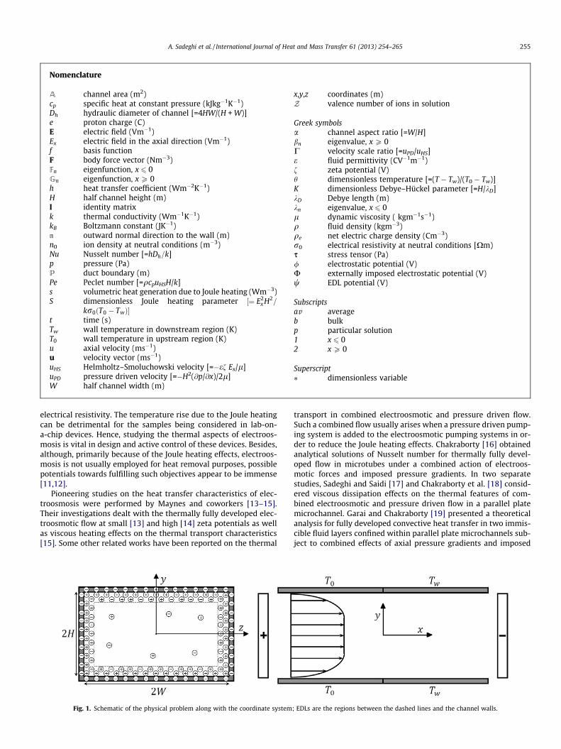
The fundamental origin of electroosmotic transport lies in thefact that when a surface is brought into contact with an electrolytesolution, it may assume a net charge. Due to the electroneutralityprinciple, the liquid takes on an opposite charge in the electric dou-ble layer (EDL) near the surface. The electric double layer, shownschematically in Fig. 1, contains an immobile inner layer and an

ll rights reserved..065

(A. Sadeghi), saman@sharif.suman@mech.iitkgp.ernet.in

outer diffuse layer [2]. If an electric field is applied tangentiallyalong the surface, a force will be exerted on the ions within the mo-bile diffuse electric layer resulting in their motion [3]. Owing toviscous drag, the liquid is drawn by the ions and therefore flowstangent to the surface. Such a fluid flow, which was explored abouttwo centuries ago [4], is referred to as electroosmotic flow.

The study of electroosmotic flow in microchannels can betraced to 1960s. One of the first attempts in this context was car-ried out by Burgreen and Nakache [5] who theoretically analyzedthe electrokinetic flow in ultrafine capillary slits. Rice and White-head [6] investigated the fully developed electroosmotic flow ina narrow cylindrical capillary for low zeta potentials, using theDebye–Hückel linearization. Subsequently, Levine et al. [7] ex-tended the Rice and Whitehead’s work to high zeta potentials bymeans of an approximation method. More recently, Kang et al.[8] analytically investigated electroosmotic flow through an annu-lus under the situation when the two cylindrical walls carry highzeta potentials. Analytical solutions for fully developed electroos-motic flow in rectangular and semicircular microchannels werepresented by Yang [9] and Wang et al. [10], respectively.

Unlike the hydrodynamic features, the study of the thermal fea-tures of electroosmosis is recent. The majority of the researchworks performed in this area deals with Joule heating effect, a phe-nomenon which arises from the applied electric field and fluid

Nomenclature

A channel area (m2)cp specific heat at constant pressure (kJkg�1K�1)Dh hydraulic diameter of channel [=4HW/(H + W)]e proton charge (C)E electric field (Vm�1)Ex electric field in the axial direction (Vm�1)f basis functionF body force vector (Nm�3)Fn eigenfunction, x 6 0Gn eigenfunction, x P 0h heat transfer coefficient (Wm�2K�1)H half channel height (m)I identity matrixk thermal conductivity (Wm�1K�1)kB Boltzmann constant (JK�1)n outward normal direction to the wall (m)n0 ion density at neutral conditions (m�3)Nu Nusselt number [=hDh=k]p pressure (Pa)P duct boundary (m)Pe Peclet number [=qcpuHSH/k]s volumetric heat generation due to Joule heating (Wm�3)S dimensionless Joule heating parameter ½¼ E2

x H2=

kr0ðT0 � TwÞ�t time (s)Tw wall temperature in downstream region (K)T0 wall temperature in upstream region (K)u axial velocity (ms�1)u velocity vector (ms�1)uHS Helmholtz–Smoluchowski velocity [=�ef Ex/l]uPD pressure driven velocity [=�H2(@p/@x)/2l]W half channel width (m)

x,y,z coordinates (m)Z valence number of ions in solution

Greek symbolsa channel aspect ratio [=W/H]bn eigenvalue, x P 0C velocity scale ratio [=uPD/uHS]e fluid permittivity (CV�1m�1)f zeta potential (V)h dimensionless temperature [=(T � Tw)/(T0 � Tw)]K dimensionless Debye–Hückel parameter [=H/kD]kD Debye length (m)kn eigenvalue, x 6 0l dynamic viscosity ( kgm�1s�1)q fluid density (kgm�3)qe net electric charge density (Cm�3)r0 electrical resistivity at neutral conditions [Xm)s stress tensor (Pa)/ electrostatic potential (V)U externally imposed electrostatic potential (V)w EDL potential (V)

Subscriptsav averageb bulkp particular solution1 x 6 02 x P 0

Superscript⁄ dimensionless variable

A. Sadeghi et al. / International Journal of Heat and Mass Transfer 61 (2013) 254–265 255

electrical resistivity. The temperature rise due to the Joule heatingcan be detrimental for the samples being considered in lab-on-a-chip devices. Hence, studying the thermal aspects of electroos-mosis is vital in design and active control of these devices. Besides,although, primarily because of the Joule heating effects, electroos-mosis is not usually employed for heat removal purposes, possiblepotentials towards fulfilling such objectives appear to be immense[11,12].

Pioneering studies on the heat transfer characteristics of elec-troosmosis were performed by Maynes and coworkers [13–15].Their investigations dealt with the thermally fully developed elec-troosmotic flow at small [13] and high [14] zeta potentials as wellas viscous heating effects on the thermal transport characteristics[15]. Some other related works have been reported on the thermal

Fig. 1. Schematic of the physical problem along with the coordinate system

transport in combined electroosmotic and pressure driven flow.Such a combined flow usually arises when a pressure driven pump-ing system is added to the electroosmotic pumping systems in or-der to reduce the Joule heating effects. Chakraborty [16] obtainedanalytical solutions of Nusselt number for thermally fully devel-oped flow in microtubes under a combined action of electroos-motic forces and imposed pressure gradients. In two separatestudies, Sadeghi and Saidi [17] and Chakraborty et al. [18] consid-ered viscous dissipation effects on the thermal features of com-bined electroosmotic and pressure driven flow in a parallel platemicrochannel. Garai and Chakraborty [19] presented a theoreticalanalysis for fully developed convective heat transfer in two immis-cible fluid layers confined within parallel plate microchannels sub-ject to combined effects of axial pressure gradients and imposed

; EDLs are the regions between the dashed lines and the channel walls.

256 A. Sadeghi et al. / International Journal of Heat and Mass Transfer 61 (2013) 254–265

electrical fields. In a recent study, Sadeghi et al. [20] reported theresults of a numerical investigation on temperature dependent ef-fects on mixed electroosmotic and pressure driven flows. The mostrecent work of this research group deals with both analytical andnumerical investigation of the hydrodynamic and thermal charac-teristics of mixed flow in a microannulus [21].

The problem of hydrodynamically fully developed and ther-mally developing flow in a channel, with the assumptions of con-stant fluid properties and negligible energy dissipation andstreamwise conduction effects is known as the Graetz problem[22,23]. Since its original solution, the Graetz problem has servedas an archetypal convective heat transfer problem both from a pro-cess modeling and an educational point of view. The classical Gra-etz problem assumes a uniform inlet temperature, shown here asT0. However, in microflows, because of the axial conduction effects,the fluid temperature is affected by the wall temperature, shownhere as Tw, even before entering the channel [24–29]. In this case,all can be said is that the fluid temperature is uniform at T0 awayfrom the entrance. Therefore, the solution domain should be ex-tended to include the upstream region and a wall temperatureshould be considered for this section. The assumed temperatureshould be consistent with the condition that the fluid temperatureaway from the entrance is T0 which turns out in a wall temperatureof T0. The wall temperature therefore should contain a step changefrom T0 to Tw at the channel inlet to physically imitate the thermalentrance condition. The previous explanation is for the case with-out internal heating; however, for extending the Graetz problem toelectroosmotic flow, one also should take into account the temper-ature distribution caused by the Joule heating.

There are some research works which extend the Graetz prob-lem to electroosmotic flow in microchannels. Nevertheless, themajority of these studies assume a uniform inlet temperature.Dutta and coworkers [30–32] extended the Graetz problem to elec-troosmotic and also mixed electroosmotic and pressure drivenflow through two dimensional straight microchannels for bothclassical boundary conditions of constant wall temperature andconstant wall heat flux. Broderick et al. [33] numerically analyzedthe thermally developing electroosmotic flow in circular micro-tubes for both constant wall heat flux and constant wall tempera-ture boundary conditions. Iverson et al. [34] developed analyticalsolutions for thermally developing electroosmotic flow with van-ishing Debye length in rectangular microchannels. All the abovementioned papers assume a uniform inlet temperature. To theauthors’ best knowledge, the only research works in this contextconsidering a physically meaningful thermal condition at the chan-nel entrance have been performed by Sharma and Chakraborty[35], Dey et al. [36,37], and Sadeghi et al. [38]. These studies aredealing with mixed flow with vanishing [35] and finite [36–38] De-bye lengths in a slit microchannel.

In most lab-on-a-chip systems, the cross section of microchan-nels made by modern micromachining technology is close to arectangular shape [39,40]. However, in studying the heat transferfeatures of electroosmosis, the rectangle geometry has receivedmuch less attention compared with the circular and parallel platemicrochannels. As mentioned previously, the only study dealingwith a thermally developing electroosmotic flow in rectangularmicrochannels, performed by Iverson et al. [34], assumes a uniforminlet temperature. Furthermore, the authors represented the effectof EDL by the Helmholtz–Smoluchowski velocity which limits theiranalysis to a purely electroosmotic flow with the channel height toDebye length ratio of above 100.

The aim of the present work is to theoretically investigate thethermally developing combined electroosmotic and pressure dri-ven flow in a rectangular microchannel by considering the actualvariations of the velocity within EDL and applying a step changeto the wall temperature. The problem is considered in two semi-

infinite regions of the channel, i.e., upstream in which x � 0 anddownstream in which x P 0 and the solutions of the two regionsare then matched at x = 0. Analytical solutions in the form of infi-nite series are obtained for the electrical potential, velocity, andtemperature. For general treatment of the eigenvalue problemassociated with the thermal solution, variational calculus, havingbeen found to be more accurate as compared with similar methods[28], is employed. An analytical solution is also presented byassuming a uniform velocity profile which is valid for a purely elec-troosmotic flow with vanishing Debye length. Finally, a detaileddiscussion is performed on the obtained results by physical inter-pretation of the trends.

2. Problem formulation

2.1. Problem definition

Consideration is given to combined electroosmotic and pressuredriven flow through a long rectangular microchannel with dimen-sions given in Fig. 1. The flow is assumed to be hydrodynamicallyfully developed. The wall temperature is the constant T0 whenx < 0 and it is the constant Tw, when x > 0. In the analysis, the fol-lowing assumptions are considered:

� Thermophysical properties are constant in the whole domainincluding EDL.� The zeta potential is constant.� Liquid contains an ideal solution of fully dissociated symmetric

salt.� Wall potentials are considered low enough for Debye–Hückel

linearization to be valid.� In calculating the charge density, it is assumed that the temper-

ature variation over the entire channel is negligible comparedwith the absolute temperature. Therefore, the charge densityfield is calculated on the basis of an average temperature.

2.2. Electrical potential distribution

The electrostatic potential, /, at any point in the channel will bedescribed by superposition of the externally applied potential, U,along the channel axis, and the double layer potential, w. Usingthe coordinate system shown in Fig. 1, at the fully developed con-ditions w = w(y,z), so

/ðx; y; zÞ ¼ UðxÞ þ wðy; zÞ ð1Þ

The electrostatic potential is related to the local net charge density,qe, at certain point in the solution by the Poisson equation:

r2/ ¼ �qe

eð2Þ

where e is the permittivity constant of the solution. In general, theNernst–Planck equations should be used to relate the electriccharge density to the electrostatic potential. However, at the fullydeveloped conditions, the spatial distribution of the electric chargedensity is described by the Boltzmann equation, in spite of the factthat it assumes the thermodynamic equilibrium [41]. This is due tothe fact that, at the fully developed conditions, the velocity vectorand the ion concentration gradient are perpendicular to each other.Using the Boltzmann distribution, the electric charge density for anideal symmetric electrolyte of valence Z is given by [2]

qe ¼ �2n0eZ sinheZwkBT

� �ð3Þ

where n0 is the ion density at neutral conditions, e is the protoncharge, kB is the Boltzmann constant and T is the absolute temper-ature. Yang et al. [42] have shown that the effect of temperature on

A. Sadeghi et al. / International Journal of Heat and Mass Transfer 61 (2013) 254–265 257

the potential distribution is negligible, using extensive numericalsimulations. Therefore, the potential field and the charge densitymay be calculated on the basis of the average temperature, Tav.For a constant voltage gradient in the x -direction, Eq. (2) becomes

@2w@y2 þ

@2w@z2 ¼

2n0eZe

sinheZwkBTav

� �ð4Þ

and in the dimensionless form

@2w�

@y�2þ @

2w�

@z�2¼ K2 sinh w� ð5Þ

where w� ¼ eZw=kBTav , y⁄ = y/H, z⁄ = z/H, and K = H/kD is the dimen-sionless Debye-Hückel parameter with kD ¼ 2n0e2Z2=ekBTav

� ��1=2

being the Debye length, a measure of the extent of EDL. For lowpotentials, namely w⁄ 6 1, sinhw⁄ in the right hand side of Eq. (5)may be approximated by w⁄. This approximation is known as De-bye–Hückel linearization. It is noted that for typical values ofZ ¼ 1 and Tav = 298 K, this approximation is valid when the electri-cal potential is below 25.7 mV. Performing the Debye–Hückel line-arization and using the boundary condition of w�P ¼ f�, with P

denoting the duct boundary and f� ¼ eZf=kBTav representing thedimensionless zeta potential, we come up with the following elec-trical potential distribution

w� ¼ f�coshðKy�Þ

cosh Kþ 2f�K2

X1n¼0

ð�1Þn cosðcny�Þ coshðgnz�Þcng2

n coshðgnaÞð6Þ

where cn = (2n + 1)p/2, g2n ¼ K2 þ c2

n , and a = W/H stands for thechannel aspect ratio.

2.3. Velocity distribution

The momentum exchange through the flow field is governed bythe Cauchy equation

qDuDt¼ �rpþr � sþ F ð7Þ

in which q denotes the fluid density, p represents the pressure, s isthe stress tensor, and u and F are the velocity and body force vec-tors, respectively. Here, the body force is given by qeE withE = �r/ representing the electric field. At the fully developed con-ditions, the effects of the transverse velocity components arenegligible compared with the axial velocity component. This,accompanied by the continuity equation, that is r�u = 0, results ina velocity vector of u = [u(y,z),0,0]. Therefore, bearing in mind thatDu/Dt = 0 for a steady fully developed flow, the momentum equa-tion in the axial direction is written as

l @2u@y2 þ

@2u@z2

!¼ @p@x� qeEx ð8Þ

where l is the dynamic viscosity and Ex = � dU/dx is the externallyapplied electric field. Substituting qe from Eq. (3) and performingthe Debye–Hückel linearization, the dimensionless form of themomentum Eq. (8) may be written as

@2u�

@y�2þ @

2u�

@z�2¼ �2C� K2

f�w� ð9Þ

wherein u⁄ = u/uHS with uHS = �efEx/l being the Helmholtz–Smolu-chowski electroosmotic velocity, which is the maximum possibleelectroosmotic velocity, and C = uPD/uHS is the velocity scale ratiowhere uPD = �H2(@p/@x)/2l stands for the pressure driven velocityscale. With zero velocity at the wall, the dimensionless velocity pro-file becomes

u� ¼ 1þ Cð1� y�2Þ � w�

f�� 4C

X1n¼0

ð�1Þn cosðcny�Þ coshðcnz�Þc3

n coshðcnaÞð10Þ

2.4. Temperature distribution and Nusselt number

To predict the heat transfer characteristics, we must begin withthe fundamental physical law of energy conservation. The mathe-matical representation of this law appropriate to a fully developedelectroosmotic flow is given as

qcpu@T@x¼ k

@2T@x2 þ

@2T@y2 þ

@2T@z2

!þ s ð11Þ

where s denotes the rate of volumetric heat generation due to Jouleheating. The Joule heating term is equal to s ¼ E2

x=r with r being theliquid electrical resistivity given by [20]

r ¼ r0

cosh w�ð12Þ

in which r0 is the electrical resistivity of neutral liquid. The termcoshw⁄ in Eq. (12) accounts for the fact that the resistivity withinEDL is lower than that of neutral liquid, due to an excess of ionsclose to the surface. For low zeta potentials, the ion density every-where is not much different from that of the neutral liquid and, as aresult, the electrical resistivity is very close to r0 everywhere. Thisconclusion could also be drawn from Eq. (12) as the term coshw⁄

approaches unity for a small electrical potential. Accordingly, sincewe are dealing with low zeta potentials, the Joule heating term maybe considered as the constant value of s ¼ E2

x=r0 [14]. The energyequation can now be modified into the following dimensionlessform

u�@h@x�¼ 1

Pe2

@2h@x�2

þ @2h@y�2

þ @2h@z�2

þ S ð13Þ

with the following dimensionless parameters

x� ¼ xHPe

; Pe ¼ qcpuHSHk

; h ¼ T � Tw

T0 � Tw; S ¼ E2

x H2

kr0ðT0 � TwÞð14Þ

As noted before, the temperature field is considered in two semi-infinite regions of the channel, that is

h ¼ h1 for x� 6 0 ð15aÞh ¼ h2 for x� P 0 ð15bÞ

The corresponding boundary conditions for the dimensionless en-ergy equation are given as

h1;P ¼ 1 ð16aÞ

h2;P ¼ 0 ð16bÞ

h1jx�!�1 ¼ 1þ hp ð16cÞ

h2jx�!1 ¼ hp ð16dÞ

h1jx�¼0 ¼ h2jx�¼0 ð16eÞ

@h1

@x�

����x�¼0¼ @h2

@x�

����x�¼0

ð16fÞ

wherein hp is the solution of h at x⁄?1where the flow is thermallyfully developed. At the fully developed conditions, the entire Jouleheating is dissipated through the wall, resulting in the disappear-ance of the axial temperature variations. Therefore, hp may be ob-tained from the following differential equation

258 A. Sadeghi et al. / International Journal of Heat and Mass Transfer 61 (2013) 254–265

@2hp

@y�2þ @

2hp

@z�2þ S ¼ 0 ð17aÞ

hp;P ¼ 0 ð17bÞ

It can be shown that the solution of Eq. (17a) subject to the bound-ary condition (17b) is as follows

hp ¼S2ð1� y�2Þ þ 2S

X1n¼0

ð�1Þnþ1 cosðcny�Þ coshðcnz�Þc3

n coshðcnaÞð18Þ

For constructing the general solution of Eq. (13), the boundary con-ditions (16c) and (16d) are the key factors. They suggest that thesolutions for the upstream and downstream regions should containthe terms 1 + hp and hp, respectively. They also dictate that theremaining terms vanish at the regions far away from the entrance.This, accompanied by the general characteristics of the partial dif-ferential Eq. (13), reveals that the remaining terms should containexponential functions of the axial coordinate. Finally, our experi-ence from solving the partial differential equations remind us thatthe remaining terms should be in the form of infinite series ofeigenfunctions. The general solution of Eq. (13) in the upstreamand downstream regions is therefore written as

h1 ¼ 1þ hp þX1n¼1

AnFnðy�; z�Þek2nx� ð19aÞ

h2 ¼ hp þX1n¼1

BnGnðy�; z�Þe�b2nx� ð19bÞ

in which An and Bn are the constants of integration and kn and bn

designate the real eigenvalues associated with the eigenfunctionsFn and Gn, respectively. By substituting Eqs. (19a) and (19b) intoEq. (13) with the consideration of Eq. (17a), it is straightforwardto show that the functions Fn and Gn satisfy the following differen-tial equations

@2Fn

@y�2þ @

2Fn

@z�2þ k2

nk2

n

Pe2 � u�ðy�; z�Þ" #

Fn ¼ 0 ð20aÞ

@2Gn

@y�2þ @

2Gn

@z�2þ b2

nb2

n

Pe2 þ u�ðy�; z�Þ" #

Gn ¼ 0 ð20bÞ

with the following boundary conditions

Fn;P ¼ 0 ð21aÞGn;P ¼ 0 ð21bÞ

which are obtainable from applying the boundary conditions (16a)and (16b) to Eqs. (19a) and (19b), respectively. The fundamentalproblem is then to determine the eigenvalues kn and bn, the eigen-functions Fn and Gn, and the coefficients An and Bn. The main diffi-culty here is that the eigenfunctions Fn and Gn are not mutuallyorthogonal by referring to the standard Sturm–Liouville problem,since the eigenvalues occur nonlinearly in (20a) and (20b). How-ever, still it is possible to seek orthogonality conditions for the prob-lem and consequently obtain the coefficients An and Bn. Substitutingthe solutions (19a) and (19b) into Eqs. (16e) and (16f), which repre-sent the continuity of temperature and its first derivative at thejunction x⁄ = 0, one may obtain the following equations

1þX1n¼1

AnFnðy�; z�Þ ¼X1n¼1

BnGnðy�; z�Þ ð22aÞ

X1n¼1

k2nAnFnðy�; z�Þ ¼ �

X1n¼1

b2nBnGnðy�; z�Þ ð22bÞ

Multiplying Eq. (22a) by ðb2m=Pe2 þ u�ÞGm and integrating the resul-

tant equation over the dimensionless channel cross section, onemay obtain

ZA�

b2m

Pe2 þ u� !

GmdA� ¼ Bm

ZA�

b2m

Pe2 þ u� !

G2mdA�

�X1n¼1

An

ZA�

b2m

Pe2 þ u� !

GmFndA�

þX1

n ¼ 1ðn–mÞ

Bn

ZA�

b2m

Pe2 þ u� !

GmGndA�ð23Þ

where A� ¼ A=H2 stands for the dimensionless cross sectional area.By multiplying Eq. (20b) by Gm and subtracting it from a similarequation for Gm multiplied by Gn, and integrating the resultantequation over A�, the following relation is achieved

ðb2m � b2

nÞZ

A�

b2m þ b2

n

Pe2 þ u� !

GmGndA�

¼Z

A�Gmr� � r�Gn �Gnr� � r�Gm½ �dA�

¼Z

P�Gm

@Gn

@n��Gn

@Gm

@n�

� �dP� ð24Þ

where r⁄ = Hr, P� ¼ P=H, and n� ¼ n=H denotes the nondimen-sional form of the outward normal direction to the wall. It shouldbe pointed out that, here and in what follows, the Del operator is as-sumed to operate only in yz plane. Using the boundary condition(21b), it is straightforward to obtain the following orthogonalitycondition from Eq. (24)

ZA�

b2m þ b2

n

Pe2 þ u� !

GmGndA�¼ 0 if n – m– 0 if n ¼ m

�ð25Þ

The integral in the last term of second member of Eq. (23) can be rewrit-ten using the above orthogonality condition and Eq. (23) becomes

ZA�

b2m

Pe2 þ u� !

GmdA� ¼ Bm

ZA�

b2m

Pe2 þ u� !

G2mdA�

�X1n¼1

An

ZA�

b2m

Pe2 þ u� !

GmFndA�

�X1

n ¼ 1ðn–mÞ

Bnb2

n

Pe2

ZA�

GmGndA� ð26Þ

Furthermore, by multiplying Eq. (22b) by Gm=Pe2 and integratingover A�, we obtain

�X1n¼1

Bnb2

n

Pe2

ZA�

GmGndA� ¼X1n¼1

Ank2

n

Pe2

ZA�

GmFndA� ð27Þ

After some manipulation, Eq. (26) takes the following form, by uti-lizing Eq. (27)Z

A�

b2m

Pe2 þ u� !

GmdA� ¼ Bm

ZA�

2b2m

Pe2 þ u� !

G2mdA� þ

X1n¼1

AnFn;m

ð28Þ

where

Fn;m ¼Z

A�

k2n � b2

m

Pe2 � u� !

GmFndA� ð29Þ

The previous technique can again be used, by multiplying Eq. (22a)this time by ðk2

m=Pe2 � u�ÞFm and also utilizing similar property asgiven by Eq. (25) for Fn, resulting in the following equation

A. Sadeghi et al. / International Journal of Heat and Mass Transfer 61 (2013) 254–265 259

ZA�

k2m

Pe2 � u� !

FmdA� ¼ �Am

ZA�

2k2m

Pe2 � u� !

F2mdA� þ

X1n¼1

BnFm;n

ð30ÞIt is easy to show that Fn,m and Fm,n are zero for any m and n. Just oneshould consider two solutions Fn and Gm of Eqs. (20a) and (20b),multiplying the first one by Gm and the second one by Fn and thensubtracting and integrating over A� to obtainZ

A�Gmr� � r�Fn � Fnr� � r�Gm½ �dA�

þ ðk2n þ b2

mÞZ

A�

� k2n � b2

m

Pe2 � u� !

GmFndA�

¼Z

P�Gm

@Fn

@n�� Fn

@Gm

@n�

� �dP� þ ðk2

n þ b2mÞFn;m ¼ 0 ð31Þ

Using the boundary conditions given by Eq. (21), it is trivial to verifythat Fn,m, and in a similar way, Fm,n are zero for any m and n. Finally,from Eqs. (28) and (30) one may get the expressions for An and Bn asratios of two integrals, i.e.,

An ¼ �

RA�

k2n

Pe2 � u��

FndA�RA�

2k2n

Pe2 � u��

F2ndA�

ð32aÞ

Bn ¼

RA�

b2n

Pe2 þ u��

GndA�RA�

2b2n

Pe2 þ u��

G2ndA�

ð32bÞ

To calculate the Nusselt number, first the dimensionless bulk tem-perature should be evaluated by the following integration

hb;i ¼R

A� u�hidA�RA� u�dA�

ð33Þ

Based on the definition, the Nusselt number is written as

Nui ¼hiDh

k¼ 4HW

H þW

@Ti@n

� P;av

TP;i � Tb;i

¼ 4að1þ aÞ2

R 10

@hi@z� ðy�;aÞdy� þ

R a0

@hi@y� ð1; z�Þdz�

hP;i � hb;ið34Þ

Our formulation is now complete except for the eigenvalues kn andbn and the eigenfunctions Fn and Gn to be determined. Since we areinterested in the downstream region, only determination of bn andGn, which is the subject of the next section, suffices.

2.5. Solution of the eigenvalue problem

2.5.1. General solutionThe variational calculus procedure is chosen for treating the

eigenvalue problem (20b). According to this method, thesolution Gn of Eq. (20b) also minimizes the following integral[28]

I ¼Z

A�

@Gn

@y�

� �2

þ @Gn

@z�

� �2

� b2n

b2n

Pe2 þ u� !

G2n �

12

@2G2n

@y�2þ @

2G2n

@z�2

!" #dA�

ð35Þ

Next, Gn is considered to be composed of a complete and linearlyindependent set of basis functions fj(y⁄,z⁄) as

Gn ¼XN

j¼1

dnjfj ð36Þ

It is worth noting that the choice of the basis functions is arbitraryprovided the boundary condition (21b) is satisfied. Here, the follow-ing functionality is assumed for fj

fjðy�; z�Þ ¼ cos½ð2lj þ 1Þpy�=2� cos½ð2mj þ 1Þpz�=2a� ð37Þ

where lj = 0,1,2, � � � , mj = 0,1,2, � � � , and N = (lj,max + 1)(mj,max + 1).Following the substitution of Gn from Eq. (36) into Eq. (35), theminimization of I(dn1, dn2, � � � ,dnN) requires having

@I@dni

¼ 0 for i ¼ 1;2; � � � ;N ð38Þ

This differentiation results in the following relation

2Z

A�

@Gn

@y�@fi

@y�þ @Gn

@z�@fi

@z�� b2

nb2

n

Pe2 þ u� !

Gnfi

" #dA�

�Z

A�

@2ðGnfiÞ@y�2

þ @2ðGnfiÞ@z�2

" #dA� ¼ 0 for i ¼ 1;2; � � � ;N ð39Þ

which can be rewritten as

2Z

A�

@2Gn

@y�2þ @

2Gn

@z�2þ b2

nb2

n

Pe2 þ u� !

Gn

" #fidA�

� 2Z

A�r� � ðfir�GnÞdA�

þZ

A�r�2ðGnfiÞdA� ¼ 0 for i ¼ 1;2; � � � ;N ð40Þ

The last two terms in Eq. (40) can be written as

�2Z

A�r� � ðfir�GnÞdA� þ

ZA�r�2ðGnfiÞdA�

¼ �Z

A�r� � ðfir�GnÞ � r� � ðGnr�fiÞ½ �dA�

¼ �Z

P�fi@Gn

@n��Gn

@fi

@n�

� �dP� ð41Þ

Since both fi and Gn should satisfy the boundary condition (21b),the right-hand side of Eq. (41), and as a result, the two last termsin Eq. (40) vanish. Then, after substitution of Gn from Eq. (36) intoEq. (40), it reduces to

XN

j¼1

dnj

ZA�

@2fj

@y�2þ @2fj

@z�2

!fidA� þ b2

n

ZA�

u�fjfidA� þ b4n

Pe2

ZA�

fjfidA�

" #

¼ 0 for i ¼ 1;2; � � � ;Nð42Þ

Eq. (42) represents a system of N equations of N + 1 unknownsincluding dn1,dn2, � � � ,dnN, and bn. This equation may be written inmatrix form as

ðAþ b2Bþ b4CÞd ¼ 0 ð43Þ

wherein the symmetric matrices A, B, and C have the elements

aij ¼Z

A�

@2fj

@y�2þ @2fj

@z�2

!fidA� ð44aÞ

bij ¼Z

A�u�fjfidA� ð44bÞ

and

cij ¼Z

A�

fjfi

Pe2 dA� ð44cÞ

The vector d in Eq. (43) stands for the coefficients d1, d2, � � � ,dN.Since Eq. (43) is not a classical eigenvalue problem, it requires amodified mathematical procedure to be solved. As noted by Haji-Sheikh [28], this equation can be reduced to a classical eigenvalueproblem by introducing new vectors v and w so that w = b2d = b2v.We will therefore have the following eigenvalue problem

0 IA B

�vw

�� b2 I 0

0 �C

�vw

�¼ 0 ð45Þ

x*

Nu

10-2 10-1 100 1010

2

4

6

8

10

12

Present study

Haji-Sheikh [28]

Pe = 1, 2, 5

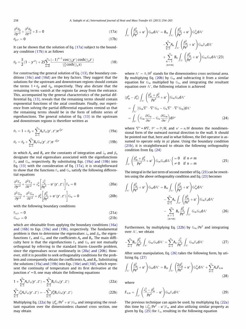
Fig. 2. Comparison between the present Nusselt numbers for the special case of thepressure driven flow with no internal heating in a square duct against thosereported by Haji-Sheikh [28].

260 A. Sadeghi et al. / International Journal of Heat and Mass Transfer 61 (2013) 254–265

where I is the identity matrix. Eq. (45) can be solved for the eigen-values b2

n and eigenvectors dn using standard computational meth-ods. It is noteworthy that since the sizes of the matrices in Eq. (45)are two times of the original ones, the solution of Eq. (45) provides2N number of the eigenvalues b2

n , N of them being positive and theothers being negative. Based on the physics of the problem, only thepositive ones can be used in calculations of the temperature field forx P 0.

2.5.2. Analytical solution for electroosmotic flow under thin EDL limitWhen the Debye length is much smaller than the channel

length scale the electroosmotic velocity profile is nearly uniformwith a large velocity gradient near the wall. Accordingly, for a highvalue of K, the velocity profile for the present problem can effi-ciently be represented by u⁄ = 1, provided no pressure gradient isapplied. By this simple velocity profile, an analytical treatment ofEq. (20b) will be possible. It is straightforward to show that theeigenfunction Gn and eigenvalue bn under a uniform velocity pro-file assumption are given as

Gn ¼ cos½ð2ln þ 1Þpy�=2� cos½ð2mn þ 1Þpz�=2a� ð46Þ

b2n ¼

PeffiffiffiffiffiffiffiffiffiffiffiffiffiffiffiffiffiffiffiffiffiffiffiffiffiffiffiffiffiffiffiffiffiffiffiffiffiffiffiffiffiffiffiffiffiffiffiffiffiffiffiffiffiffiffiffiffiffiffiffiffiffiffiffiffiffiffiffiffiffiffiffiffiffiffiffiffiffiffiffiffiPe2 þ ð2ln þ 1Þ2p2 þ ð2mn þ 1Þ2p2=a2

q� Pe2

2ð47Þ

where ln = 0,1,2,� � � and mn = 0,1,2, � � � . The following expression isalso obtained for Bn by inserting Eqs. (46) and (47) into Eq. (32b)

Table 1Comparison between the present fully developed Nusselt number values againstliterature data for the special case of purely electroosmotic flow with a ?1 andS = �1.

K Nu Error (%)

Present study Ref. [17]

5 10.5961 10.6197 0.222210 11.0750 11.0997 0.222520 11.4563 11.4818 0.222140 11.6954 11.7214 0.221880 11.8291 11.8555 0.2227

Bn ¼ 8ð�1Þlnþmn ð2mn þ 1Þ=ð2ln þ 1Þa2 þ ð2ln þ 1Þ=ð2mn þ 1Þ

Pe2 þ ð2ln þ 1Þ2p2 þ ð2mn þ 1Þ2p2=a2 � PeffiffiffiffiffiffiffiffiffiffiffiffiffiffiffiffiffiffiffiffiffiffiffiffiffiffiffiffiffiffiffiffiffiffiffiffiffiffiffiffiffiffiffiffiffiffiffiffiffiffiffiffiffiffiffiffiffiffiffiffiffiffiffiffiffiffiffiffiffiffiffiffiffiffiffiffiffiffiffiffiffiPe2 þ ð2ln þ 1Þ2p2 þ ð2mn þ 1Þ2p2=a2

q ð48Þ

3. Method validation

Before proceeding with the discussion of results, a comparisonagainst existing literature data is needed for validation of themethod developed. One of the best choices for comparison arethe data reported by Haji-Sheikh [28] for thermally developingPoiseuille flow in a rectangular duct. Since these data have beenobtained by assuming no internal heat generation, we should setS = 0. In addition, the velocity scale ratio should tend infinity forthe electroosmotic part of velocity to vanish. Moreover, the veloc-ity profile is normalized by the mean velocity because Haji-Sheikh[28] has used the mean velocity for non-dimensionalization. For abetter comparison, since he used 120 eigenvalues in the computa-tions, both lj,max and mj,max are set to 10 to provide 121 eigenvalues.Fig. 2 shows both the present Nusselt number values and those re-ported by Haji-Sheikh [28] at different Peclet numbers and revealsa good agreement between them.

Since the above comparison was for no internal heating case,one cannot be sure that the results are free of error until a com-plete check in the presence of the Joule heating is made. Table 1compares the fully developed Nusselt number values for purelyelectroosmotic flow in a channel with a large aspect ratio, that isa ?1 , against those predicted using the expression given bySadeghi and Saidi [17] for a parallel plate channel. As observed,the relative error for all the cases being considered is only about0.2% which is quite acceptable especially because the present re-sults are obtained by means of the numerical integration. Further-more, although we consider a quite large aspect ratio for thechannel to imitate a slit but there still will be corner effects in-

cluded in the calculations. It should be pointed out that the com-parison is only made for S = �1 because the research work doneby Sadeghi and Saidi [17] is generally dealing with a constant heatflux boundary condition and it only reduces to a constant temper-ature boundary condition when S = �1.

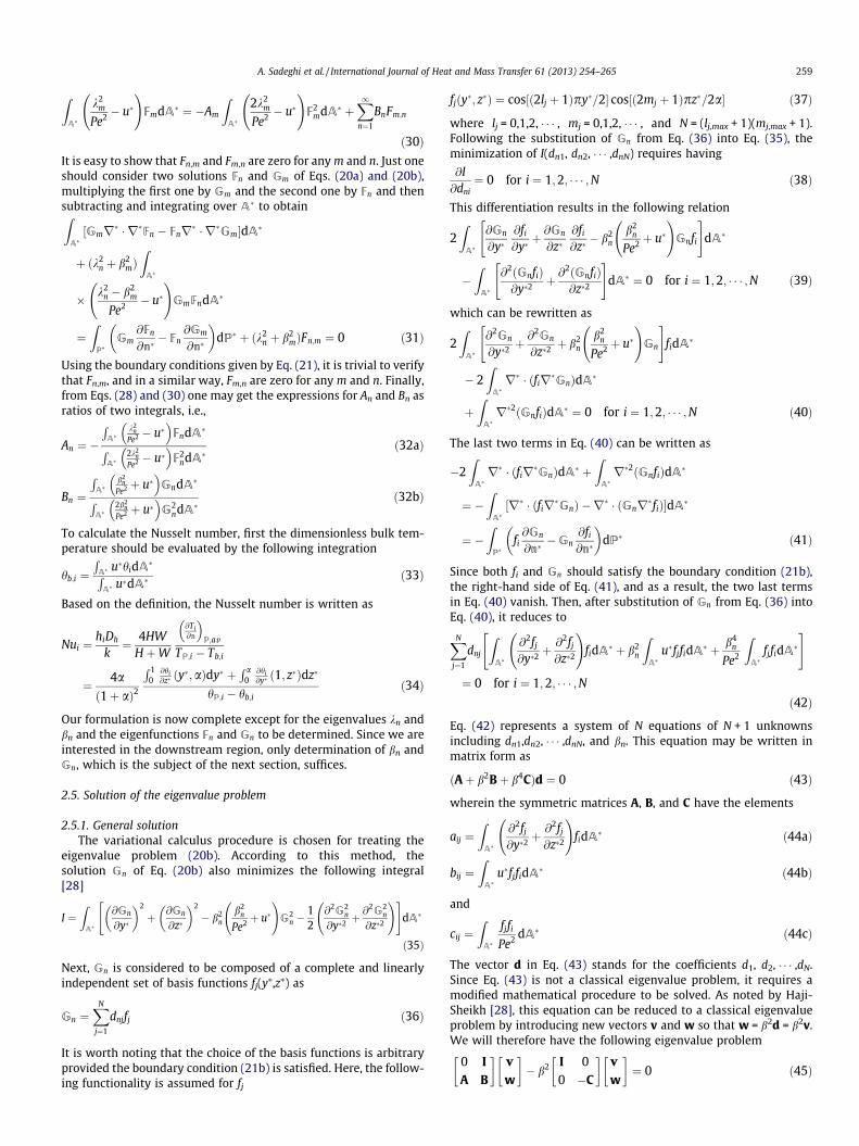
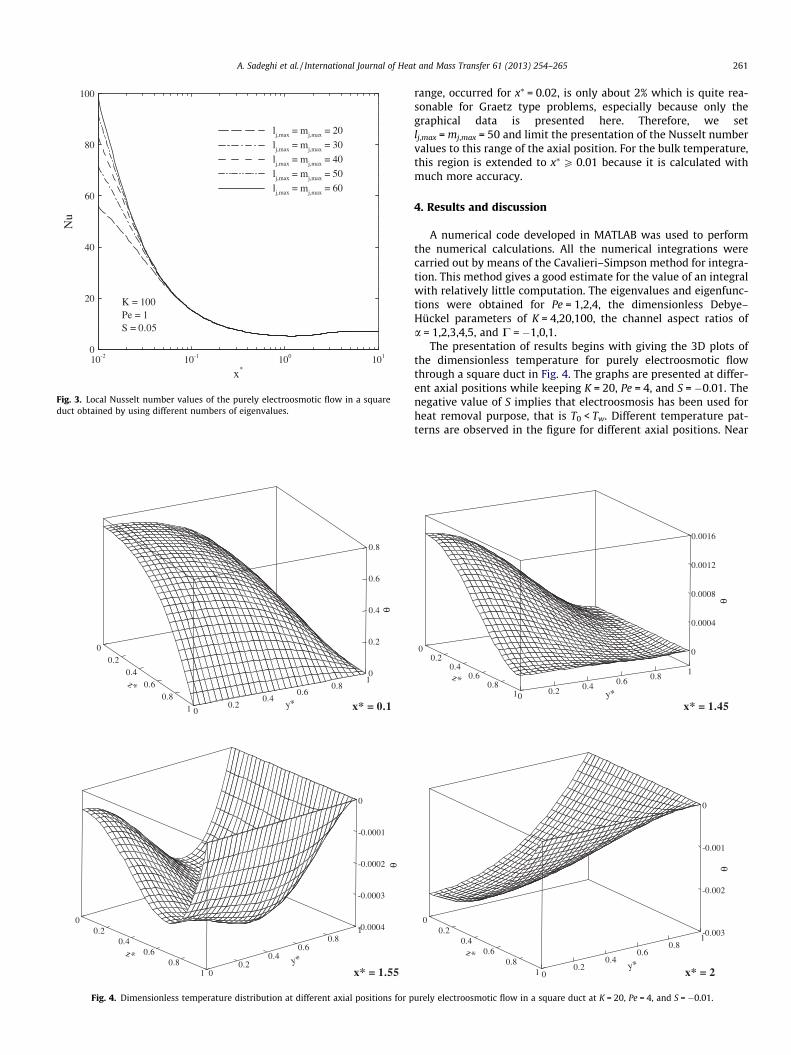
Besides the validation of results, since the convergence of theseries solution becomes more difficult by decreasing the axial po-sition, a convergence analysis is needed to find out the region inwhich the results are accurate. Fig. 3 illustrates the local Nusseltnumber values of the purely electroosmotic flow in a square ductobtained by using different numbers of eigenvalues. The data isprovided for Pe = 1, the minimum Peclet number which will beused in presenting the results, for which the error is maximum.As observed in the figure, the discrepancy between the results ob-tained by setting lj,max = mj,max = 50 and those of lj,max = mj,max = 60 isnot significant for x⁄P 0.02. The maximum discrepancy in this

x*

Nu

10-2 10-1 100 1010

20

40

60

80

100

lj,max = mj,max = 20

lj,max = mj,max = 30

lj,max = mj,max = 40

lj,max = mj,max = 50

lj,max = mj,max = 60

Κ = 100Pe = 1S = 0.05

Fig. 3. Local Nusselt number values of the purely electroosmotic flow in a squareduct obtained by using different numbers of eigenvalues.

z*

00.2

0.40.6

0.81 y*0

0.20.4

0.60.8

1

θ

0

0.2

0.4

0.6

0.8

x* = 0.1

z*

00.2

0.40.6

0.81

y*0

0.20.4

0.60.8

1

θ

-0.0004

-0.0003

-0.0002

-0.0001

0

x* = 1.55

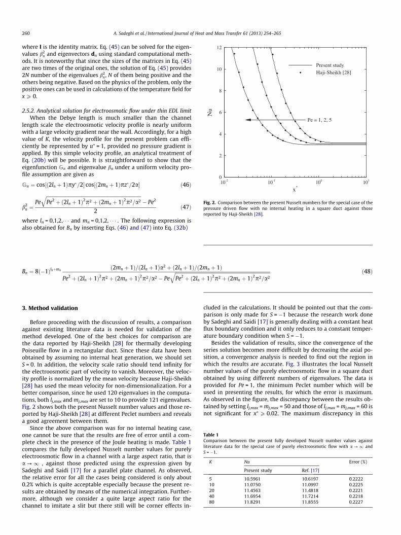
Fig. 4. Dimensionless temperature distribution at different axial positions for p

A. Sadeghi et al. / International Journal of Heat and Mass Transfer 61 (2013) 254–265 261

range, occurred for x⁄ = 0.02, is only about 2% which is quite rea-sonable for Graetz type problems, especially because only thegraphical data is presented here. Therefore, we setlj,max = mj,max = 50 and limit the presentation of the Nusselt numbervalues to this range of the axial position. For the bulk temperature,this region is extended to x⁄P 0.01 because it is calculated withmuch more accuracy.

4. Results and discussion

A numerical code developed in MATLAB was used to performthe numerical calculations. All the numerical integrations werecarried out by means of the Cavalieri–Simpson method for integra-tion. This method gives a good estimate for the value of an integralwith relatively little computation. The eigenvalues and eigenfunc-tions were obtained for Pe = 1,2,4, the dimensionless Debye–Hückel parameters of K = 4,20,100, the channel aspect ratios ofa = 1,2,3,4,5, and C = �1,0,1.

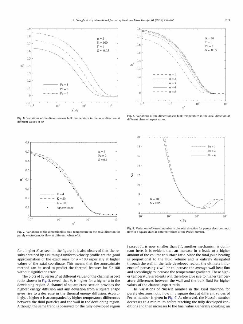
The presentation of results begins with giving the 3D plots ofthe dimensionless temperature for purely electroosmotic flowthrough a square duct in Fig. 4. The graphs are presented at differ-ent axial positions while keeping K = 20, Pe = 4, and S = �0.01. Thenegative value of S implies that electroosmosis has been used forheat removal purpose, that is T0 < Tw. Different temperature pat-terns are observed in the figure for different axial positions. Near

z*

00.2

0.40.6

0.81

y*0

0.20.4

0.60.8

1

θ

-0.003

-0.002

-0.001

0

x* = 2

z*

00.2

0.40.6

0.81 y*0

0.20.4

0.60.8

1

θ

0

0.0004

0.0008

0.0012

0.0016

x* = 1.45

urely electroosmotic flow in a square duct at K = 20, Pe = 4, and S = �0.01.

z*

00.2

0.40.6

0.81 y*0

0.20.4

0.60.8

1

θ

-0.0025

-0.002

-0.0015

-0.001

-0.0005

0

S = -0.02

z*

00.2

0.40.6

0.81

y*0

0.20.4

0.60.8

1

θ

0

0.002

0.004

0.006

0.008

S = 0.01

z*

00.2

0.40.6

0.81

y*0

0.20.4

0.60.8

1

θ

0

0.002

0.004

0.006

0.008

0.01

S = 0.02

z*

00.2

0.40.6

0.81 y*0

0.20.4

0.60.8

1

θ

-0.0002

0

0.0002

0.0004

0.0006

S = -0.01

Fig. 5. Dimensionless temperature distribution at different values of S for purely electroosmotic flow in a square duct at K = 20, Pe = 4, and x⁄ = 1.5.

262 A. Sadeghi et al. / International Journal of Heat and Mass Transfer 61 (2013) 254–265

the entrance, that is at x⁄ = 0.1, the temperature profile is of anearly parabolic shape. As expected, the temperature is lower thanTw everywhere reflecting in a positive h. This is therefore a regionin which an efficient cooling is possible. As the fluid moves down-stream its temperature is increased because of cooling the walland, as a result, the wall heat flux decreases gradually. This reduc-tion is continued until x⁄ ffi 1.45 at which the average wall heat fluxvanishes. This point, corresponding to x ffi 6H, is the end of thecooled section of the duct and the rest of channel is left uncooled.Although for higher axial positions the wall heat flux is negative,i.e., heat is transferred from the fluid to the wall, the fluid temper-ature is increased due to the Joule heating. It should be pointed outthat the negative wall heat flux in this region is not significant andit therefore will not cause a problem in cooling purposes. In fact, byassuming a temperature difference of 20K between the inlet fluidand the wall, the maximum temperature difference between thewall and the fluid at the fully developed conditions will be onlyabout 0.06K. Hence, the associated wall heat flux will be negligibleand the duct and the fluid may be assumed to be in the thermalequilibrium.

Fig. 5 depicts the dimensionless temperature distribution at dif-ferent values of S for purely electroosmotic flow in a square duct atK = 20, Pe = 4, and x⁄ = 1.5. As seen, while the case of S = �0.01 isjust at the end of the cooled section of the duct, the case ofS = �0.02 has by far passed this section. This reveals that it is pos-sible to increase the cooled section of the duct by decreasing theJoule heating rate. In an expected behavior, a higher Joule heating

effect is accompanied by higher dimensionless temperatures forthe surface heating cases, that is for positive values of S.

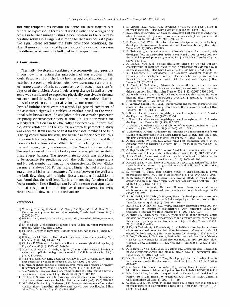
The variations of the dimensionless bulk temperature in the ax-ial direction at different values of Peclet number is presented inFig. 6. The axial coordinate has been multiplied by Pe in order toremove its Peclet number dependency. As observed, the bulk tem-perature is a decreasing function of the axial coordinate. In thedeveloping region, a smaller Peclet number corresponds to a lowerdimensionless temperature at a given axial position. This is due tothe fact that, a decrease in Peclet number, which may be thought ofas a decrease in velocity, gives the fluid particles the opportunity tosense the wall effects more by means of the thermal energy diffu-sion. This higher effect of energy diffusion, therefore, causes athicker thermal boundary layer and consequently a smaller entrylength for a lower Peclet number, as observed in the figure. Allthe graphs merge together in the fully developed region, emphasiz-ing the fact that the fully developed temperature distribution inthe presence of internal heating is independent of Peclet number.

Fig. 7 illustrates the variations of the dimensionless bulk tem-perature in the axial direction for purely electroosmotic flow at dif-ferent values of the dimensionless Debye–Hückel parameter. Thepredictions of the approximate method are also shown by symbols.By increasing K, EDL will be limited to smaller regions adjacent tothe wall, resulting in higher velocities near the wall. Accordingly,the weight of the fluid particles near the wall, having smallernon-dimensional temperatures, in calculating hb is increased,resulting in smaller values of the dimensionless bulk temperature

x*Pe

θ b

10-2 10-1 100 101-0.1

0

0.1

0.2

0.3

0.4

0.5

0.6

0.7

0.8

0.9

Pe = 1

Pe = 2

Pe = 4

α = 2Κ = 100Γ = 1S = -0.05

Fig. 6. Variations of the dimensionless bulk temperature in the axial direction atdifferent values of Pe.

x*

θ b

10-2 10-1 100 1010

0.1

0.2

0.3

0.4

0.5

0.6

0.7

0.8

Κ = 4Κ = 20Κ = 100Approximate

α = 2Pe = 2S = 0.1

Fig. 7. Variations of the dimensionless bulk temperature in the axial direction forpurely electroosmotic flow at different values of K.

x*

θ b

10-2 10-1 100 101-0.1

0

0.1

0.2

0.3

0.4

0.5

0.6

0.7

0.8

α = 1α = 2α = 3α = 4α = 5

Κ = 20Γ = 1Pe = 2S = -0.05

Fig. 8. Variations of the dimensionless bulk temperature in the axial direction atdifferent channel aspect ratios.

x*Pe

Nu

10-2 10-1 100 1014

6

8

10

12

14

16

18

20

Pe = 1

Pe = 2

Pe = 4

Κ = 100S = 0.05

Fig. 9. Variations of Nusselt number in the axial direction for purely electroosmoticflow in a square duct at different values of the Peclet number.

A. Sadeghi et al. / International Journal of Heat and Mass Transfer 61 (2013) 254–265 263

for a higher K, as seen in the figure. It is also observed that the re-sults obtained by assuming a uniform velocity profile are the goodapproximation of the exact ones for K = 100 especially at highervalues of the axial coordinate. This means that the approximatemethod can be used to predict the thermal features for K > 100without significant error.

The plots of hb versus x⁄ at different values of the channel aspectratio, shown in Fig. 8, reveal that hb is higher for a higher a in thedeveloping region. A channel of square cross section provides thehighest energy diffusion and any deviation from a square shapegives rise to a decrease in the thermal energy diffusion. Accord-ingly, a higher a is accompanied by higher temperature differencesbetween the fluid particles and the wall in the developing region.Although the same trend is observed for the fully developed region

(except Tw is now smaller than Tb), another mechanism is domi-nant here. It is evident that an increase in a leads to a higheramount of the volume to surface ratio. Since the total Joule heatingis proportional to the fluid volume and is entirely dissipatedthrough the wall in the fully developed region, the ultimate influ-ence of increasing a will be to increase the average wall heat fluxand accordingly to increase the temperature gradients. These high-er temperature gradients will therefore give rise to higher temper-ature differences between the wall and the bulk fluid for highervalues of the channel aspect ratio.

The variations of Nusselt number in the axial direction forpurely electroosmotic flow in a square duct at different values ofPeclet number is given in Fig. 9. As observed, the Nusselt numberdecreases to a minimum before reaching the fully developed con-ditions and then increases to the final value. Generally speaking, an

264 A. Sadeghi et al. / International Journal of Heat and Mass Transfer 61 (2013) 254–265

increase in Peclet number is accompanied by a decrease in Nusseltnumber in the developing region. The wall heat flux is an increas-ing function of the Peclet number; therefore, this trend of Nusseltnumber is due to higher temperature differences between the walland liquid particles for higher Peclet numbers. The functionality ofthe wall heat flux with Peclet number may be considered as a par-adox at first glance, as the wall heat flux at each axial position ishigher, whereas still higher temperature differences between thewall and fluid particles exist for higher Peclet numbers. However,attention should be given to the fact that a higher Peclet numbermay be thought of as a higher mass flow rate and consequently ahigher energy storage capacity.

The variations of Nu in the axial direction at different values ofK, given in Fig. 10, show that the Nusselt number is higher for ahigher value of the dimensionless Debye–Hückel parameter. As

x*

Nu

10-2 10-1 100 1010

5

10

15

20

25

30

Κ = 4Κ = 20Κ = 100Approximate

α = 2Pe = 2S = 0.1

Fig. 10. Variations of Nusselt number in the axial direction for purely electroos-motic flow at different values of K.

x*

Nu

10-2 10-1 100 1010

5

10

15

20

25

30

α = 1α = 2α = 3α = 4α = 5

Κ = 20Γ = −1Pe = 2S = 0.1

Fig. 11. Variations of Nusselt number in the axial direction at different values of a.

noted previously, the dimensionless bulk temperature is a decreas-ing function of K. Furthermore, a higher K is accompanied by ahigher wall heat flux because of higher velocities near the wall.This higher wall heat flux along with a smaller hb for a higher valueof the dimensionless Debye–Hückel parameter are the causes ofincreasing Nu with K. Fig. 10 also leads one to the following conclu-sion: similar to the dimensionless bulk temperature, the Nusseltnumbers obtained by means of the approximate method are suffi-ciently accurate for K > 100.

Fig. 11 depicts the Nusselt number values versus the dimen-sionless axial coordinate at different values of the channel aspectratio. Unlike the previous cases which were dealing with eitherof a purely electroosmotic flow or a pressure assisted flow, thatis the case for which C > 0, this figure presents the results for apressure opposed flow. From Fig. 8, one may expect a decreasingtrend of Nu with increasing a. However, it can be seen in Fig. 11that the opposite is true, that is an increase in a gives rise to a high-er Nu. This is mainly because of increasing Dh, the length scale usedin calculation of Nu, with increasing a. Furthermore, as noted be-fore, the ratio of the total Joule heating to the channel surface ishigher for a higher value of the channel aspect ratio resulting inhigher amounts of the wall heat flux and, accordingly, higher Nus-selt number values.

So far, we have limited the presentation of the Nusselt numbersto positive values of S. Fig. 12 illustrates the local Nusselt numbervalues of a square duct at different velocity scale ratios for a neg-ative S. It is observed that singularities occur in Nusselt numbervalues. For a better explanation of this phenomenon, we makeuse of Fig. 4. When entering the channel, the fluid starts to beheated from the wall. The wall heat flux is thus from the wall tothe fluid and the Nusselt number is positive. As the fluid is beingheated, the average wall heat flux decreases gradually and reacheszero at some axial position (x⁄ ffi 1.45 for the case shown in Fig. 4),providing a zero Nusselt number. From this point forward, thedirection of the wall heat flux changes due to the internal heating.However, still the bulk temperature is below the wall temperature,and, as a result, the Nusselt number is negative. In spite of the factthat the fluid is being cooled from the wall, the bulk temperatureincreases due to the internal heating, resulting in a higher Nusseltnumber with negative sign. In the limit Tb ? Tw, the Nusselt num-ber with negative sign goes to infinity. At the point that the wall

x*

Nu

10-2 10-1 100 101-5

0

5

10

15

20

Γ = −1Γ = 0Γ = 1

Κ = 100Pe = 2S = -0.1

Fig. 12. Nusselt number values of a square duct versus x⁄ at different values of C.

A. Sadeghi et al. / International Journal of Heat and Mass Transfer 61 (2013) 254–265 265

and bulk temperatures become the same, the heat transfer ratecannot be expressed in terms of Nusselt number and a singularityoccurs in Nusselt number values. More increase in the bulk tem-perature results in a large value of the Nusselt number with posi-tive sign. Before reaching the fully developed conditions, theNusselt number is decreased by increasing x⁄ because of increasingthe difference between the bulk and wall temperatures.

5. Conclusions

Thermally developing combined electroosmotic and pressuredriven flow in a rectangular microchannel was studied in thiswork. Because of both the Joule heating and axial conduction ef-fects being present in electroosmotic flows, assuming a uniform in-let temperature profile is not consistent with actual heat transferphysics of the problem. Accordingly, a step change in wall temper-ature was considered to represent physically conceivable thermalentrance conditions. Expressions for the dimensionless distribu-tions of the electrical potential, velocity, and temperature in theform of infinite series were presented. For general treatment ofthe associated eigenvalue problem, a method based on the varia-tional calculus was used. An analytical solution was also presentedfor purely electroosmotic flow at thin EDL limit for which thevelocity distribution can be efficiently described by a uniform pro-file. After validation of the results, a complete parametric studywas executed. It was revealed that for the cases in which the fluidis being cooled from the wall, the Nusselt number decreases to aminimum before reaching the fully developed conditions and thenincreases to the final value. When the fluid is being heated fromthe wall, a singularity is observed in the Nusselt number values.The mechanism of this singularity point was explained in detailusing energy balance. The approximate solution was also foundto be accurate for predicting both the bulk mean temperatureand Nusselt number as long as the dimensionless Debye–Hückelparameter is above 100. Furthermore, a higher channel aspect ratioguarantees a higher temperature difference between the wall andthe bulk flow along with a higher Nusselt number. In addition, itwas found that the wall heat flux is an increasing function of thePeclet number. These findings can be of immense consequence inthermal design of lab-on-a-chip based microsystems involvingelectroosmotic flow actuation mechanisms.

References

[1] X. Wang, S. Wang, B. Gendhar, C. Cheng, C.K. Byun, G. Li, M. Zhao, S. Liu,Electroosmotic pumps for microflow analysis, Trends Anal. Chem. 28 (1)(2009) 64–74.

[2] R.F. Probstein, Physicochemical Hydrodynamics, second ed., Wiley, New York,1994.

[3] J.H. Masliyah, S. Bhattacharjee, Electrokinetic Colloid Transport Phenomena,first ed., Wiley, New Jersey, 2006.

[4] F.F. Reuss, Charge-induced flow, Proc. Imperial Soc. Nat. Mosc. 3 (1809) 327–344.

[5] D. Burgreen, F.R. Nakache, Electrokinetic flow in ultrafine capillary slits, J. Phys.Chem. 68 (5) (1964) 1084–1091.

[6] C.L. Rice, R. Whitehead, Electrokinetic flow in a narrow cylindrical capillary, J.Phys. Chem. 69 (11) (1965) 4017–4024.

[7] S. Levine, J.R. Marriott, G. Neale, N. Epstein, Theory of electrokinetic flow in finecylindrical capillaries at high zeta-potentials, J. Colloid Interface Sci. 52 (1)(1975) 136–149.

[8] Y. Kang, C. Yang, X. Huang, Electroosmotic flow in a capillary annulus with highzeta potentials, J. Colloid Interface Sci. 253 (2) (2002) 285–294.

[9] D. Yang, Analytical solution of mixed electroosmotic and pressure-driven flowin rectangular microchannels, Key Eng. Mater. 483 (2011) 679–683.

[10] C.Y. Wang, Y.H. Liu, C.C. Chang, Analytical solution of electro-osmotic flow in asemicircular microchannel, Phys. Fluids 20 (6) (2008) 063105.

[11] P.F. Eng, P. Nithiarasu, O.J. Guy, An experimental study on an electro-osmoticflow-based silicon heat spreader, Microfluid. Nanofluid. 9 (4–5) (2010) 787–795.

[12] M.F. Al-Rjoub, A.K. Roy, S. Ganguli, R.K. Banerjee, Assessment of an active-cooling micro-channel heat sink device, using electro-osmotic flow, Int. J. HeatMass Transfer 54 (21–22) (2011) 4560–4569.

[13] D. Maynes, B.W. Webb, Fully developed electro-osmotic heat transfer inmicrochannels, Int. J. Heat Mass Transfer 46 (8) (2003) 1359–1369.

[14] B.C. Liechty, B.W. Webb, R.D. Maynes, Convective heat transfer characteristicsof electro-osmotically generated flow in microtubes at high wall potential, Int.J. Heat Mass Transfer 48 (12) (2005) 2360–2371.

[15] D. Maynes, B.W. Webb, The effect of viscous dissipation in thermally fully-developed electro-osmotic heat transfer in microchannels, Int. J. Heat MassTransfer 47 (5) (2004) 987–999.

[16] S. Chakraborty, Analytical solutions of Nusselt number for thermally fullydeveloped flow in microtubes under a combined action of electroosmoticforces and imposed pressure gradients, Int. J. Heat Mass Transfer 49 (3–4)(2006) 810–813.

[17] A. Sadeghi, M.H. Saidi, Viscous dissipation effects on thermal transportcharacteristics of combined pressure and electroosmotically driven flow inmicrochannels, Int. J. Heat Mass Transfer 53 (19–20) (2010) 3782–3791.

[18] R. Chakraborty, D. Chakraborty, S. Chakraborty, Analytical solution forthermally fully developed combined electroosmotic and pressure-drivenflows in narrow confinements with thick electrical double layers, J. HeatTransfer 133 (2) (2011).

[19] A. Garai, S. Chakraborty, Micro-scale thermo-fluidic transport in twoimmiscible liquid layers subject to combined electroosmotic and pressure-driven transport, Int. J. Heat Mass Transfer 52 (11–12) (2009) 2660–2666.

[20] A. Sadeghi, H. Yavari, M.H. Saidi, S. Chakraborty, Mixed electroosmotically andpressure-driven flow with temperature- dependent properties, J. Thermophys.Heat Transfer 25 (3) (2011) 432–442.

[21] H. Yavari, A. Sadeghi, M.H. Saidi, Hydrodynamic and thermal characteristics ofcombined electroosmotic and pressure driven flow in a microannulus, J. HeatTransfer 134 (10) (2012) 101703.

[22] L. Graetz, Uber die warmeleitungsfahigheit von flussingkeiten: Part 1, Annalender Physik und Chemie 252 (1882) 79–94.

[23] L. Graetz, Uber die warmeleitungsfahigheit von flussingkeiten: Part 2, Annalender Physik und Chemie 261 (1885) 337–357.

[24] J. Lahjomri, A. Oubarra, Analytical solution of the Graetz problem with axialconduction, J. Heat Transfer 121 (4) (1999) 1078–1083.

[25] J. Lahjomri, A. Oubarra, A. Alemany, Heat transfer by laminar Hartmann flow inthermal entrance eregion with a step change in wall temperatures: The Graetzproblem extended, Int. J. Heat Mass Transfer 45 (5) (2002) 1127–1148.

[26] A. Haji-Sheikh, J.V. Beck, D.E. Amos, Axial heat conduction effects in theentrance region of parallel plate ducts, Int. J. Heat Mass Transfer 51 (25–26)(2008) 5811–5822.

[27] A. Haji-Sheikh, J.V. Beck, D.E. Amos, Axial heat conduction effects in theentrance region of circular ducts, Heat Mass Transfer 45 (3) (2009) 331–341.

[28] A. Haji-Sheikh, Determination of heat transfer in ducts with axial conductionby variational calculus, J. Heat Transfer 131 (9) (2009) 091702.

[29] A. Haji-Sheikh, W.J. Minkowycz, S. Manafzadeh, Axial conduction effect in flowthrough circular porous passages with prescribed wall heat flux, Heat MassTransfer 46 (7) (2010) 727–738.

[30] K. Horiuchi, P. Dutta, Joule heating effects in electroosmotically drivenmicrochannel flows, Int. J. Heat Mass Transfer 47 (14–6) (2004) 3085–3095.

[31] K. Horiuchi, P. Dutta, A. Hossain, Joule-heating effects in mixed electro-osmotic and pressure-driven microflows under constant wall heat flux, J. Eng.Math. 54 (2) (2006) 159–180.

[32] P. Dutta, K. Horiuchi, H.M. Yin, Thermal characteristics of mixedelectroosmotic and pressure-driven microflows, Comput. Math. Appl. 52 (5)(2006) 651–670.

[33] S.L. Broderick, B.W. Webb, D. Maynes, Thermally developing electro-osmoticconvection in microchannels with finite debye-layer thickness, Numer. HeatTransfer. Part A: Appl. 48 (10) (2005) 941–964.

[34] B.D. Iverson, D. Maynes, B.W. Webb, Thermally developing electroosmoticconvection in rectangular microchannels with vanishing Debye-layerthickness, J. Thermophys. Heat Transfer 18 (4) (2004) 486–493.

[35] A. Sharma, S. Chakraborty, Semi-analytical solution of the extended Graetzproblem for combined electroosmotically and pressure-driven microchannelflows with step-change in wall temperature, Int. J. Heat Mass Transfer 51 (19–20) (2008) 4875–4885.

[36] R. Dey, D. Chakraborty, S. Chakraborty, Extended Graetz problem for combinedelectroosmotic and pressure-driven flows in narrow confinements with thickelectric double layers, Int. J. Heat Mass Transfer 55 (17–18) (2012) 4724–4733.

[37] R. Dey, T. Ghonge, S. Chakraborty, Steric-effect-induced alteration of thermaltransport phenomenon for mixed electroosmotic and pressure driven flowsthrough narrow confinements, Int. J. Heat Mass Transfer 56 (1–2) (2013) 251–262.

[38] A. Sadeghi, H. Veisi, M.H. Saidi, S. Chakraborty, Graetz problem extended tomixed electroosmotically and pressure-driven flow, J. Thermophys. HeatTransfer 26 (1) (2012) 123–133.

[39] X.Y. Chen, K.C. Toh, J.C. Chai, C. Yang, Developing pressure-driven liquid flow inmicrochannels under the electrokinetic effect, Int. J. Eng. Sci. 42 (5–6) (2004)609–622.

[40] H.A. Stone, A.D. Stroock, A. Ajdari, Engineering flows in small devices:Microfluidics toward a lab-on-a-chip, Ann. Rev. Fluid Mech. 36 (2004) 381–411.

[41] H.M. Park, J.S. Lee, T.W. Kim, Comparison of the Nernst-Planck model and thePoisson–Boltzmann model for electroosmotic flows in microchannels, J.Colloid Interface Sci. 315 (2) (2007) 731–739.

[42] C. Yang, D. Li, J.H. Masliyah, Modeling forced liquid convection in rectangularmicrochannels with electrokinetic effects, Int. J. Heat Mass Transfer 41 (24)(1998) 4229–4249.