Vaulin pohang 2010

Outline

1

APCTP Pohang ,Korea, July 26 – 30, 2010Special credit to Sanghoon Oh

Interpreting results of gravitational-wave search: from

detection to astrophysicsRuslan Vaulin

University of Wisconsin-Milwaukee

APCTP Pohang ,Korea, July 26 – 30, 2010

2

Outline

• Sources of transient gravitational-wave signals.

• Generic search.

• Working example: search for CBC in S5/VSR1 data paper.

- Introduction and Data Quality

- Pipeline: tuning and detection statistic

- Results: detection candidates

- Interpretation: upper limits on rates of CBC

- Appendix: blind injection challenge

• Summary

3


References

4


• [low mass LV paper]: arXiv:1005.4655

• [FINDCHIRP paper]: arXiv:gr-qc/0509116

• [Rates paper]: arXiv:1003.2480

• [Tuning paper]: http://www.ligo.caltech.edu/docs/T/T070109-01.pdf

• [Galaxy paper]: http://arxiv.org/abs/0706.1283

• [Inspiral Search Interpretation paper]: http://arxiv.org/abs/0707.2410

• [Loudest event statistic paper]: http://arxiv.org/abs/0710.0465

Transient gravitational-wave signals

5


• Definition: transient signals are the signals whose duration is much smaller than a typical observation time.

• Signal duration depends on the source and detector’s noise curve.

• Typical duration in S5: 100 ms - 45 seconds

• Expected duration in advanced detectors: up to 30 minutes.

Sources of transient gravitational-wave signals

6


• Compact binary coalescence (CBC):

- neutron star - neutron star (BNS)

- neutron star - black hole (NSBH)

- black hole - black hole (BBH)

• Core-collapse supernova

• Cosmic string cusps

• Unknown transient sources of gravitational radiation

Compact binary coalescence - simple picture

7


• Binary systems of massive compact objects in close orbits: neutron stars (NS) and/or black holes (BH).• Orbits decay by radiating energy as gravitational waves.• Objects eventually collide and merge.

Real CBCs

8


• Spin modulates the waveform, its effect are more significant for high mass unequal mass ratio systems.

• Orbits for most systems are expected to be circularized by the time they are in detector’s sensitive band.

• Predictions for CBC rates have large uncertainties.

• Astrophysics of neutron stars is very complicated and sensitive to unknown microphysics. Equation of state is not known.

• Within the Einstein’s theory of general relativity coupled to “classical” matter, black holes are “clean” objects.

• Real black holes may turned out to be quite different!

Inspiral waveform

9


Deff = D!F 2

+

"1 + cos2ı

2

#2

+ F 2!cos2ı

$"1/2

h(t) =! GMc

c2Deff

"! tc ! t

5GMc/c3

"!1/4cos[2!0 ! 2!(t! tc,Mc, ")]

Mc =(m1m2)3/5

(m1 + m2)1/5

(m1, m2,!s1,!s2, e, tc, "0)(D,!, ", ı, #)

• CBC is described by a set of extrinsic and intrinsic parameters:

• The restricted Post-Newtonian inspiral waveform measured by a detector can be written as [FINDCHIRP paper]:

where

Effective Distance

Chirp mass

Inspiral waveforms in LIGO/Virgo Detectors

10


GW signal from a1.4,1.4 Msun

Binary Neutron Star Systemfisco =

c3

6!

6GM" 4397Msun

M

• The ending frequency of inspiral stage is well approximated by the frequency of ISCO:

• The part of inspiral signal in the sensitive band is determined by flow (of the detector) and fISCO.

• For systems with M > 35 Msun it is essential to include merger and ringdown ( EOBNR waveforms)

• For initial LIGO/Virgo CBC signals naturally split into: low mass (2 - 35), high mass (35 - 100), ringdown (100 - 500).

Predicted Rates for CBC

11


[Rates paper]

Generic search: inference

12


• Formulate the question. This most often can be mapped to determining a measurable quantity . For example: rate of binary neutron star coalescence.

• Choose a probabilistic model that assign probability of finding particular set of data if is realized in nature.

• Use Bias theorem to infer posterior probability for given the experimental data:

p(!|data) ! p(data|!)p(!)

!!

!

Generic search: detection

13


• In the case of continues observations targeting transient gravitational wave signals most of the experimental data are noise.

• In most cases of interest, useful information about astrophysics of the sources can be infer only from the segments of data that contain gravitational wave signal.

• Thus, it is natural for continuously running observations to split inference process into two stages:

- Detection: identification of segments of data with signals

- Parameter estimation: inference of astrophysical parameters from the reduced set of data

• Important exception: Null result. To be discussed in detail.

Generic search: detection problem

14


• Optimal detection strategy requires evaluation of likelihood ratio:

!(data, signal) =p(data|signal)p(data|noise)

• In the case of stationary and Gaussian noise, it corresponds to match-filter with template waveforms, and standard signal-to-noise ratio (SNR):

! =!

s!(f)h(f)Sn(f)

• For multiple identical detectors network it becomes a coherent sum of SNR’s

Generic search: Ranking candidates

15


• In the regime of weak signals we have to rely on statistical detection

• First, we search for signals in the data recording plausible candidates (triggers).

• Then, we sort the plausible candidates (segments) based on their likelihood to be gravitational wave signal.

• In the search for family of signals, Optimal ranking is given by the marginalized likelihood ratio, which is normally approximated by its maximum.

• For convenience, detection or ranking statistic is introduced, which is a monotonic function of likelihood ratio or its approximation.

Generic search: background estimation

16


• The sorted list of candidate events may contain strong and weak signals and noise artifacts.

• In order to identify truly significant candidates (and possibly claim detection) the observed candidates must be compared with a list of triggers typically found in the background.

• This last step ultimately determines level of significance of the measured candidates: the more rare the candidate the more significant it is.

• It is convenient to map ranking statistic into inverse rate of false alarms ( IFAR) which is an invariant measure of significance.

Generic search: summary

17


1. Search data for significant triggers. Reduce the number of triggers to process by applying hard threshold cuts and vetoes.

2. Rank triggers by likelihood ratio (detection or ranking statistic).

3. Estimate background.

4. Compare zero-lag triggers to background by calculating false alarm rate for every trigger.

5. Evaluate detection efficiency by injecting simulated signals into that data.

6. Estimate parameters (in case of detection), calculate upper limits, do astrophysics, test predictions of GR, measure deviations from GR, extract new physics.

S5/VSR1 low mass CBC search paper: outline

18


I. Introduction.

II. Data quality.

III. The data analysis pipeline.

IV. Results: detection candidates.

V. Results.

II. Upper limits.

III. Appendix.

[low mass LV paper]

I. Introduction.

19


• Network: H1, H2, L1, V1

- Hanford, Washington, USA: H1, H2

- Livingston, Louisiana, USA: L1

- Cascina, Italy: V1

• S5: November 2005 – October 2007

• VSR1: May 2007 - October 2007

• Searched last 5 months

• low mass, up 35 Msun CBC

II.Data quality

20


5 10 15 20 25 30 35Total Mass (M!)

0

50

100

150

200

250

Insp

iralH

oriz

onD

ista

nce

(Mpc

)

H1H2L1V1

• Detectors have different sensitivities.

• Detectors are sensitive to their environment.

• There are gaps in data, quality of data varies.

• Account for 11 possible detector combinations ( e.g. H1L1, H1L1V1 etc).

• Inspiral horizon distance is the distance at which an optimally located, optimally oriented binary would produce triggers with SNR of 8 in the detector.

Fig 1. [low mass LV paper]

21


II.Data quality: DQ vetoes

• Science data: detector is in lock operating properly.

• Category N data: Science data with DQ vetoes up to category N applied

• Segments of the science data that were labeled as category N or lower DQ veto are excluded.

• Categories of DQ vetoes :

- Category 1: severe problems,

- Category 2: noise artifacts with well understood origin and coupling,

- Category 3: likely noise artifacts based on statistical correlations,

- Category 4: least serious problems, used in the follow-up of the candidates.

22


II.Data quality: analysis times

• Analysis time indicates that the listed detectors are collecting science-quality data.

III.Overview of the analysis pipeline

23


• Credit: Romain Gouaty, see his lecture slides for more details

24


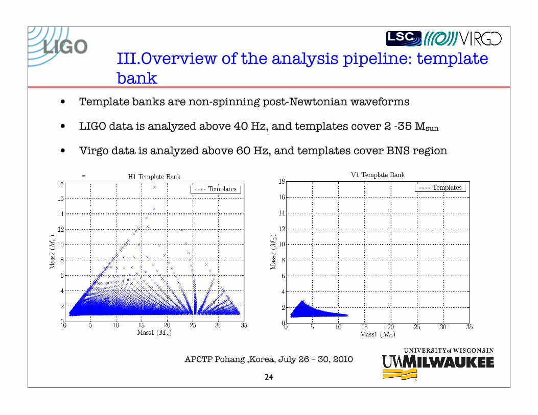
III.Overview of the analysis pipeline: template bank

• Template banks are non-spinning post-Newtonian waveforms

• LIGO data is analyzed above 40 Hz, and templates cover 2 -35 Msun

• Virgo data is analyzed above 60 Hz, and templates cover BNS region

-

25


III.Overview of the analysis pipeline: background

• Background is estimated by time sliding data from different detectors with respect to each other.

• We performed 100 time-shifts: equivalent to 100 experiments of the same duration.

• The time shifts: L1 is 10 seconds, V1 is 15 seconds, H1 and H2 are not shifted.

• H1 and H2 are collocated.

• Time-shifted data are processed as the actual unshifted data.

• It allows us to estimated rates of accidental coincidences of the noise glitches.

26


III.Overview of the analysis pipeline: tuning thresholds

• Thresholds introduce in the pipeline to get rid of clear noise artifacts thus reducing amount of triggers to process downstream.

• Ideal cut is along the line of the constant likelihood ratio, which is normally not calculated at early stages of the pipeline

• We apply several thresholds and cuts that (even though sub-optimal) are guarantee to result in improved sensitivity.

• Definition: The process of choosing types and parameters of the cuts accompanied by verification of their efficiency is called tuning. [Tuning paper]

27


III.Overview of the analysis pipeline: detection statistic in Gaussian noise

• Optimal detection strategy requires evaluation of likelihood ratio:

!(data, signal) =p(data|signal)p(data|noise)

• In the case of stationary and Gaussian noise, it corresponds to match-filter with template waveforms, and standard signal-to-noise ratio (SNR):

! =!

s!(f)h(f)Sn(f)

• For multiple identical detectors network it becomes a coherent sum of SNR’s

28


• Real noise is not stationary and has a strong non-Gaussian component.

• Detectors are not identical.

• Due to environmental disturbances detectors fall out of science mode.

• The quality of data is not uniform: detectors are sensitive to their environment.

III.Overview of the analysis pipeline: real noise

29


III.Overview of the analysis pipeline: SNR thresholds

• For multiple detectors network in Gaussian stationary noise optimal statistic is coherent sum of SNR’s

!c(t) = !1(t) + !2(t! "(#,$))

• But real noise has long non-Gaussian tales

• We remove them by imposing SNR thresholds at the level of individual detectors and then test for coincidence, calculate combined statistic etc. • Credit: Lisa Goggin, S4 data

30


III.Overview of the analysis pipeline: tuning chi-squared veto threshold

• To reject noise artifacts, we use signal-based vetoes.

• Chi-squared test measures deviation of the observed signal from the template waveform

31


III.Overview of the analysis pipeline: tuning coincidence window

• We require triggers from different detectors to be coincident in time and mass parameters.

• In the process of tightening the window we check that detection efficiency does not decrease.

32


III.Overview of the analysis pipeline: evolution of detection statistic in CBC searches

• Goal: estimate likelihood ratio

• Use as much information (parameters) about triggers as possible

• Measure background distribution

• Measure foreground distribution

• The goal is to develop new detection statistic through corrections of SNR approaching with every new search actual likelihood ratio - the optimal statistic.

• SNR -> effective SNR -> IFAR -> Effective likelihood, GRB likelihood ...

33


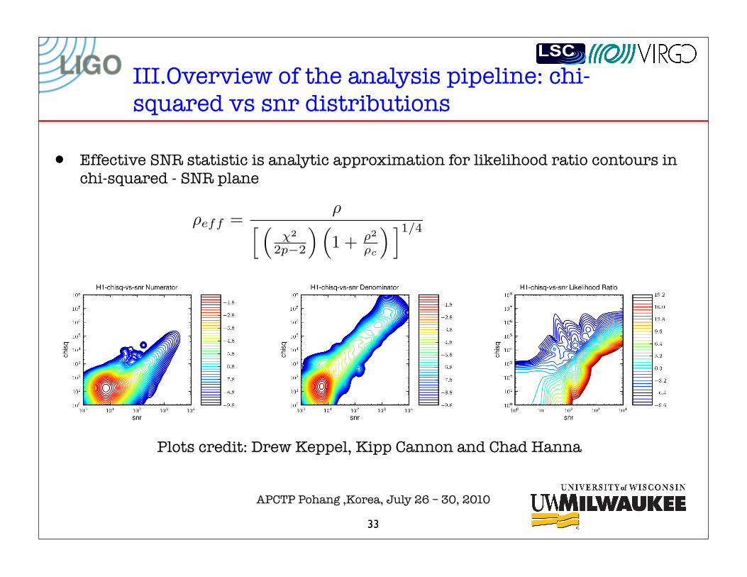
Plots credit: Drew Keppel, Kipp Cannon and Chad Hanna

III.Overview of the analysis pipeline: chi-squared vs snr distributions

!eff =!

! "!2

2p!2

# "1 + "2

"c

# $1/4

• Effective SNR statistic is analytic approximation for likelihood ratio contours in chi-squared - SNR plane

34


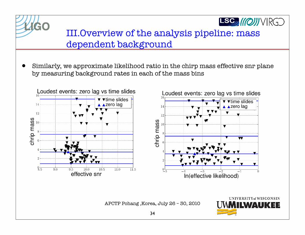
III.Overview of the analysis pipeline: mass dependent background

• Similarly, we approximate likelihood ratio in the chirp mass effective snr plane by measuring background rates in each of the mass bins

35


• We use simulated signals added to the real data to estimate likelihood of detection for every detector combination and every type of the trigger.

!(",#) =!

found D3inj!

all D3inj

.

III.Overview of the analysis pipeline: efficiency factors

H1L1 in H1H2L1V1

H1L1 in H1L1V1

H1L1 in H1H2L1

H1L1 in H1L1

H1H2L1 in H1H2L1V1

where ! and " are the event typeand analysis time

• Define efficiency factor:

36


III.Overview of the analysis pipeline: Effective likelihood

L(!c, m,", #) = ln!

$(",#)R0(!c, m,", #)

"

where !(",#) - e!ciency factor,R0($c, ", #) - background rate,(",#) - trigger type and analysis time.m - chirp mass bin

• Combining efficiency factor with background rates into likelihood like ratio we define detection statistic for the search to be:

37


Missed/Found injections with effective SNR

38


Missed/Found injections with effective likelihood

Detection efficiency

39

GR19, Mexico City, 2010

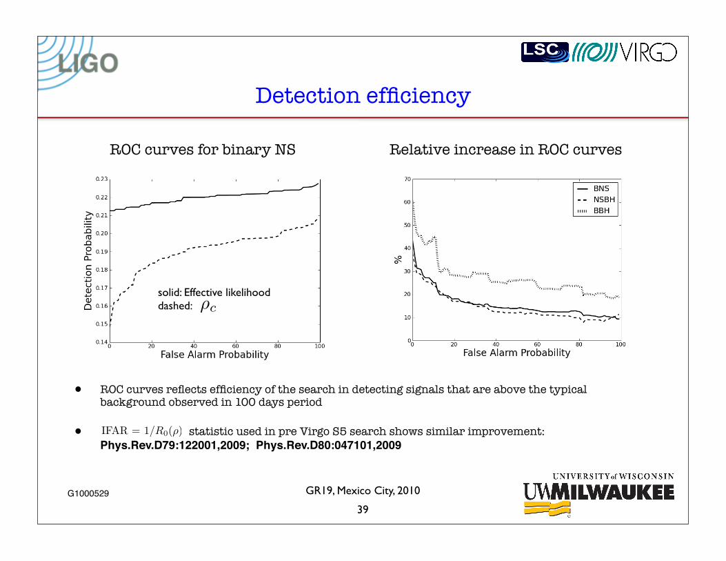
ROC curves for binary NS Relative increase in ROC curves

solid: Effective likelihooddashed:

• ROC curves reflects efficiency of the search in detecting signals that are above the typical background observed in 100 days period

• statistic used in pre Virgo S5 search shows similar improvement: Phys.Rev.D79:122001,2009; Phys.Rev.D80:047101,2009IFAR = 1/R0(!)

!c

G1000529

40


IV.Results: false alarm rate (FAR)

• Definition: Define FAR(L) as number of background triggers with detection statistic >= L divided by duration of background data

• FAR can be defined for any statistic or search algorithm and, once it is calculated, provides invariant measure of significance of the candidate.

• Any statistic can be mapped to 1/FAR or IFAR

• It is convenient to present results on a diagram using IFAR

41


IV.Results: IFAR diagram

Fig2. [low mass LV paper]

42


IV.Results: Loudest event

• We find no events with a detection statistic significantly larger than the background estimation in CAT 3 data

• The loudest trigger in the five-month span is an H1L1 coincidence from H1H2L1V1 time with a false alarm rate of 19 per year. As 0.28 year was searched, this is consistent with the background expectation.

• We also examined CAT 2 data and found no significant candidates,

• Except...

Appendix: Blind Injection Challenge

43

GR19, Mexico City, 2010

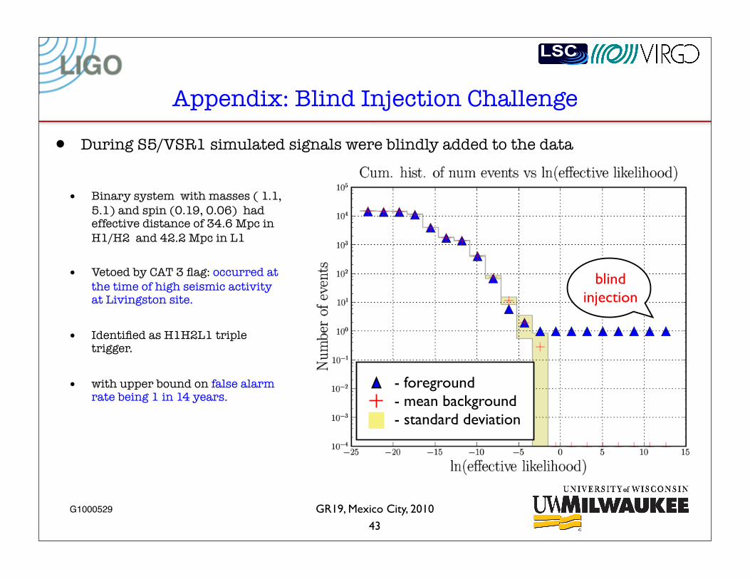
• During S5/VSR1 simulated signals were blindly added to the data

• Binary system with masses ( 1.1, 5.1) and spin (0.19, 0.06) had effective distance of 34.6 Mpc in H1/H2 and 42.2 Mpc in L1

• Vetoed by CAT 3 flag: occurred at the time of high seismic activity at Livingston site.

• Identified as H1H2L1 triple trigger.

• with upper bound on false alarm rate being 1 in 14 years.

- foreground- mean background- standard deviation

blind injection

G1000529

V.Upper limits: Rate of CBC

44


• Goal: based on results of experiment estimate rate, , of binary coalescence

• is measured in number of coalescence per year per L10.

• L10 is 1010 times the blue solar luminosity, which is expected to be proportional to the binary coalescence rate

• We would like to estimate rates for the following objects:

• Given null result we calculate upper limits on rates.

BNS: [m1 = m2 = (1.35± 0.04) Msun],BHNS: [m1 = (5± 1) Msun, m2 = (1.35± 0.04) Msun],BBH: [m1 = m2 = (5± 1) Msun].

µ

µ

45


V.Upper limits: Loudest event method

p(x|µ) =dP (x|µ)

dx

p(µ|x) ! p(x|µ)p(µ)

• Data: the loudest event found by the search with detection statistic x

• First, calculate cumulative probability of observing no events louder then x in experiment of duration T for a given value of rate of coalescence :

• Cl(x) is combined luminosity of galaxies “visible” above x.

• Likelihood is then:

• Finally, apply Bayes theorem to get posterior distirbution:

P (x|µ) = e!µClT Pb(x)µ

See [Loudest event statistic paper] for more ....

46


V.Upper limits: posterior probability distribution

p (µ|CL, T,!) =CLT

1 + !(1 + µCLT!) e!µCLT

! (x) =!! 1CL

dCL

dx

" !1P0

dP0

dx

"!1

where µ is the rate and T is the analyzed time. In general, ! is given by

• Posterior for uniform prior is given by

• Results of the previous searches are incorporated as priors through multiplying probabilities distributions and normalizing the final posterior:

p(µ|S5, S4, S3, ...) ! p(µ|S5)p(µ|S4)p(µ|S3)...

p(µ)

47


V.Upper limits: posterior probability distribution for BNS

• Fig3. [low mass LV paper]

48


V.Upper limits: upper limits

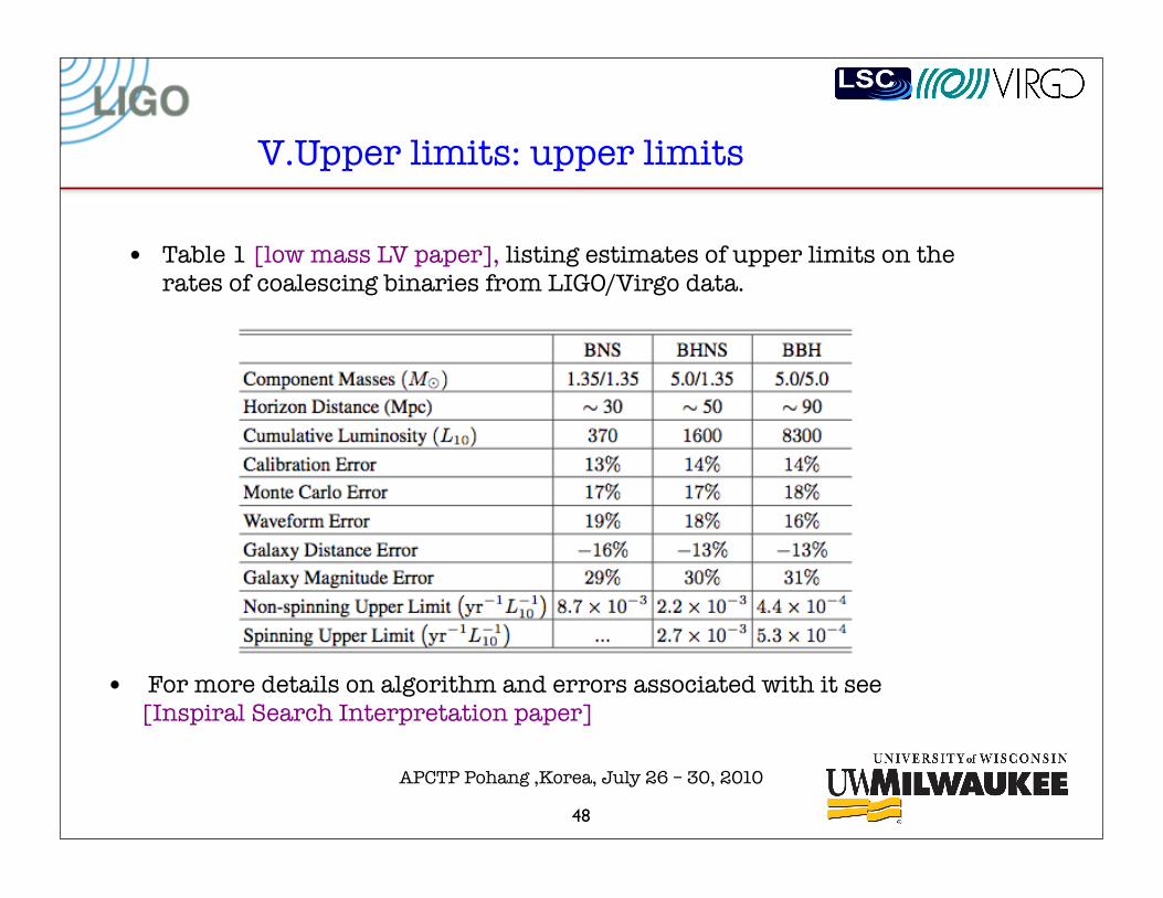
• Table 1 [low mass LV paper], listing estimates of upper limits on the rates of coalescing binaries from LIGO/Virgo data.

• For more details on algorithm and errors associated with it see [Inspiral Search Interpretation paper]

49


V.Upper limits: upper limits compared to realistic expected atrophysical rates

• Credit: Duncan Brown

50


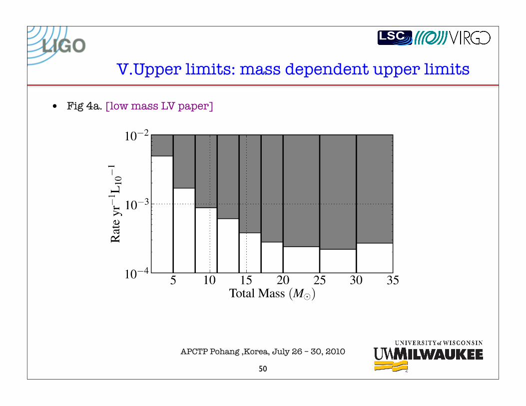
V.Upper limits: mass dependent upper limits

• Fig 4a. [low mass LV paper]

51


V.Upper limits: dependence of upper limit on component mass

• Fig 4b. [low mass LV paper]

Outline

52


Date post:	14-Jul-2015
Category:	Documents
Upload:	luckyph
View:	153 times
Download:	0 times

Vaulin pohang 2010

Documents