Appendix A – Assumptions ......................................................................................................... 29
Appendix B – Additional Tables .................................................................................................. 35
Appendix C - Model Chart Summary .......................................................................................... 38
Works Cited ................................................................................................................................. 39
Curriculum Vitae ......................................................................................................................... 42
4
iv. List of Tables Table 1 Standard Deviation of Demand ........................................................................................ 11 Table 2 Forecasted Generation Summary .................................................................................... 24 Table 3 Electric Grid Emissions Summary ..................................................................................... 25 Table 4 Vehicle Emissions Summary ............................................................................................. 26 Table 5 Total Emissions Summary ................................................................................................. 27 Table 6. PJM Load Distribution ..................................................................................................... 35 Table 7. 2020 Base Case Dispatch Model ..................................................................................... 35 Table 8 Base Load NG Supply ........................................................................................................ 36 Table 9 Peaking Natural Gas Supply.............................................................................................. 36 Table 10 Electric Vehicle Count - On the Road ............................................................................. 37
5
v. List of Figures Figure 1 Research Methodology Flow Chart .................................................................................... 9 Figure 2 Demand Volatility ............................................................................................................ 11 Figure 3 Base Case 2020 ................................................................................................................ 12 Figure 4 Base Case - 2030 ............................................................................................................. 13 Figure 5 Base Case - 2040 ............................................................................................................. 14 Figure 6 Base Case - 2050 ............................................................................................................. 15 Figure 7 TOU Case – 2020 ............................................................................................................. 16 Figure 8 TOU Case – 2030 ............................................................................................................. 17 Figure 9 TOU Case – 2050 ............................................................................................................. 18 Figure 10 TOU Case – 2050 ........................................................................................................... 19 Figure 11 V2G Case – 2020 ........................................................................................................... 20 Figure 12 V2G Case – 2030 ........................................................................................................... 21 Figure 13 V2G Case – 2040 ........................................................................................................... 22 Figure 14 V2G Case – 2050 ........................................................................................................... 23
6
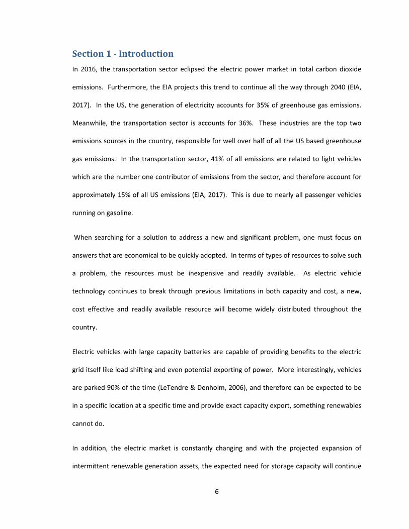
Section 1 - Introduction In 2016, the transportation sector eclipsed the electric power market in total carbon dioxide
emissions. Furthermore, the EIA projects this trend to continue all the way through 2040 (EIA,
2017). In the US, the generation of electricity accounts for 35% of greenhouse gas emissions.
Meanwhile, the transportation sector is accounts for 36%. These industries are the top two
emissions sources in the country, responsible for well over half of all the US based greenhouse
gas emissions. In the transportation sector, 41% of all emissions are related to light vehicles
which are the number one contributor of emissions from the sector, and therefore account for
approximately 15% of all US emissions (EIA, 2017). This is due to nearly all passenger vehicles
running on gasoline.
When searching for a solution to address a new and significant problem, one must focus on
answers that are economical to be quickly adopted. In terms of types of resources to solve such
a problem, the resources must be inexpensive and readily available. As electric vehicle
technology continues to break through previous limitations in both capacity and cost, a new,
cost effective and readily available resource will become widely distributed throughout the
country.
Electric vehicles with large capacity batteries are capable of providing benefits to the electric
grid itself like load shifting and even potential exporting of power. More interestingly, vehicles
are parked 90% of the time (LeTendre & Denholm, 2006), and therefore can be expected to be
in a specific location at a specific time and provide exact capacity export, something renewables
cannot do.
In addition, the electric market is constantly changing and with the projected expansion of
intermittent renewable generation assets, the expected need for storage capacity will continue
7
to grow to support continuous and safe delivery of electricity. Expansion of electric vehicles can
play a major role in not just providing a more secure power source, but have the benefit of
reducing emissions both from the grid and from replacement of gasoline power vehicles.
The purpose of this research paper and complementary model is to identify the true emissions
savings from a full electric vehicle compared to gasoline fueled vehicles now and in the future.
The benefits of electric vehicles can be larger than anticipated, and, as an ancillary benefit,
improve the overall efficiency of both the electric and transportation sectors.
It is anticipated that benefits to utilities by deploying electric vehicles include an increased load
factor (average demand divided by peak demand) and reduced cycling of facilities (LeTendre &
Denholm, 2006). These improvements to the generation supply should also reduce emissions by
the grid on a per unit of electricity basis by improving overall efficiency of operations.
Therefore, when considering time of use and vehicle-to-grid in the emissions portfolio of an
electric vehicle, electric vehicle net emissions should be reduced even further as well as the
overall emissions efficiency of the electric generation itself will show improvement.
The model created considers two main scenarios that are further explained below. It is
important to note that one scenario considers “vehicle-to-grid” technology, the idea that high
capacity car batteries can act as distributed energy resources. Vehicle-to-grid in this model is
assumed as a pure net metering opportunity. Many studies believe that the best aspects of
vehicle-to-grid are actually in the ancillary electric markets like frequency regulation and
demand response. However, due to differences in interstate system operators across the
country of which the treatment of these benefits is not uniform, no ancillary markets are
considered.
8
Section 2 - Methods The objective of the model was to recreate a national perspective that could estimate time-of-
use and emissions on an hourly basis. This required two priority considerations: creating a
national daily demand curve and a national daily dispatch model. By completing these priorities,
an effective model could be created to estimate hourly emissions more accurately to consider
when an electric vehicle is charging or dispatching power in a V2G scenario.
To create a demand curve, the PJM ISO is assumed as the national standard for demand shape.
By taking five years of hourly historical data from 2012 through and including 2016, the average
load per hour over 5 years was calculated. The average load per hour was then divided by the
entire average daily load to create a percentage of load for the day in any given hour. This
demand distribution creates a demand shape that can be reutilized for a national scale. This
shape can be seen in Table 5. PJM Load Distribution in Appendix B – Additional Tables.
The EIA’s 2017 Annual Energy Outlook (“AEO”) forecasts national demand on an annual basis
out to 2050. The annual demand can then be put into the PJM demand distribution to create a
daily demand curve of national energy use. In the model, the demand actually demonstrates
the total billion kWh utilized in a specific hour of the day throughout the entire year, so that if
the 24 hours of the day are aggregated, it would equal to total national annual demand in billion
kWh. This creates a shape and a curve that can be filled in with the available generation options
with annual data from the AEO to demonstrate what generation technology is employed and
when.
As previously mentioned, the AEO includes annual generation projections by generation
technology out to 2050. Therefore, utilizing certain dispatch rules outlined in the Appendix A –
Assumptions, a dispatch curve was created that prioritized renewables, base load technologies,
9
and peaking technologies, in that order. With this dispatch model, one can estimate the
emissions in CO2 equivalent per kWh in any given hour on a national scale. An example if the
dispatch model can be found in Appendix B – Additional Tables demonstrating the EIA Reference
Case for 2020 (Table 6. 2020 Base Case Dispatch Model).
The diagram below outlines the data analyzed to create the final emissions projections.
After the demand curve and dispatch model are created, assumptions can be made on when an
electric vehicle is charged and provide a more accurate estimate of the emissions tied to the
electricity consumed during that time. The expected result should be more accurate than a
national emission per kWh average that does not consider time of use. The Time of Use
Scenario (“TOU Scenario”) estimates the emissions savings by converting gasoline vehicles to
electric vehicles and the emissions from the power charging the electric vehicle from the
Demand Curve
Supply Forecast
PJM Historical
Data
EIA Demand Forecast
EIA Generation Forecast
ERCOT Historical
Wind
NREL PVWatts Forecast
Dispatch Model
Grid Emissions
TOU Case
V2G Case
BEV Inputs
Charging Inputs
CAFÉ Standard
s
Light Vehicle
Fleet
Vehicle Emissions
Total Emissions
Figure 1 Research Methodology Flow Chart
10
generation technologies dispatched during the time the battery is charged. The Vehicle-to-Grid
Scenario (“V2G Scenario) takes this model iteration further. The V2G scenario considers the
emissions per kWh during the charging as well as the emissions per kWh of the power it
replaces when the battery in the electric vehicle is dispatching power to the electric grid.
To calculate the emissions savings, there are multiple ways to interpret the data. First, an
estimate is created to calculate the emissions in the grid itself as the dispatched technologies
change according to demand and load shape to support expansion of electric vehicles. This can
be added to a transportation emissions savings estimate by converting gasoline vehicles to non-
emitting electric vehicles to create a total emissions savings value. Second, a per vehicle
emissions calculation is created to estimate the impact on a smaller scale of converting a
gasoline vehicle to an electric vehicle in both the TOU and V2G Scenarios compared to a base
BEV scenario that does not consider TOU or V2G, but an average grid emissions in total.
Section 3 - Results The following is a summary of the demand curves and dispatch models for all three scenarios:
Base Case, TOU Case and V2G Case. The emissions results are summarized at the end of the
section. Each case is projected for snapshots in 2020, 2030, 2040 and 2050. Please see the
Appendix A – Assumptions to review what is assumed to build out the projected dispatch
models.
3.1 Demand Volatility To calculate volatility, a standard deviation was taken of each scenario demand forecast for a
given year. The standard deviation allows the measurement of volatility by quantifying the
variation among the values. The lower a standard deviation is indicates less variation in values.
It would be assumed that lower standard deviations align with less volatility and better
11
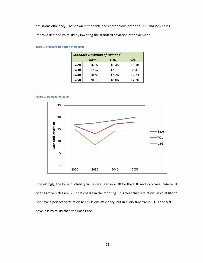
emissions efficiency. As shown in the table and chart below, both the TOU and V2G cases
improve demand volatility by lowering the standard deviation of the demand.
Table 1 Standard Deviation of Demand
Standard Deviation of Demand Base TOU V2G 2020 16.97 16.45 15.18 2030 17.62 13.17 8.41 2040 18.81 17.26 14.33 2050 20.11 18.06 14.30
Figure 2 Demand Volatility
Interestingly, the lowest volatility values are seen in 2030 for the TOU and V2G cases, where 9%
of all light vehicles are BEV that charge in the morning. It is clear that reductions in volatility do
not have a perfect correlation to emissions efficiency, but in every timeframe, TOU and V2G
have less volatility than the Base Case.
-
5
10
15
20
25
2020 2030 2040 2050
Stan
dard
Dev
iatio
n
Base
TOU
V2G
12
3.2 Base Case The Base Case assumes EIA projections on both generation resources and total demand while
utilizing the PJM demand curve shape.
Figure 3 Base Case 2020
The Base Case 2020 is a great reference case that is closest to the current energy environment.
It’s easy to see that both coal and nuclear are large parts of the dispatch model. Additionally,
natural gas generation comes mostly in the form of peaking natural gas, a less efficient
application. Solar, wind and other renewables are all prioritized in dispatch due to their
intermittent nature.
This shape shows a true on and off peak model with inefficient technologies like single cycle
natural gas, petroleum and pumped storage meeting the peak demand hours of the day.
The average CO2e emissions are 419 g/kWh. The top power producing resource is coal.
-
50
100
150
200
250
300
HE01
HE03
HE05
HE07
HE09
HE11
HE13
HE15
HE17
HE19
HE21
HE23
Annu
al D
eman
d (b
illio
n kW
h)
Time of Day
Natural Gas, Excess Supply
Petroleum, Pumped Storage, &Other DG
Natural Gas, Peaking
Coal
Natural Gas
Nuclear
Solar
Wind
13
Figure 4 Base Case - 2030
The Base Case 2030 begins to demonstrate the impact of renewable expansion. Wind growth
generally pushes the entire curve upward, but solar creates a mid-day “hump” in the dispatch
model. This “hump” can cause inefficiency in the natural gas generation dispatch, as more
peaking natural gas will be required once the sun goes down on the solar arrays, an issue
currently experience in CAISO commonly referred to as the “Duck Curve” (CAISO, 2016).
As demand grows, base load natural gas capacity has improved from 26% to 40% of all natural
gas generation. This creates a more emissions efficiency in the dispatch model.
The average CO2e emissions are 354 g/kWh. The top power producing resource is coal.
-
50
100
150
200
250
300
HE01
HE03
HE05
HE07
HE09
HE11
HE13
HE15
HE17
HE19
HE21
HE23
Annu
al D
eman
d (b
illio
n kW
h)
Time of Day
Natural Gas, Excess Supply
Petroleum, Pumped Storage, &Other DG
Natural Gas, Peaking
Coal
Natural Gas
Nuclear
Solar
Wind
14
Figure 5 Base Case - 2040
The Base Case 2040 shows the electric market to continue to shift to renewables and base load
natural gas generation. Renewables in this scenario account for 27% of all generation across the
U.S. and the combined natural gas technologies account for 38% of all generation.
Of the natural gas generation, over 52% will be base load generation by 2040. The increasing
renewables and base load natural gas create greater emissions efficiencies.
When considering nuclear and all renewables, over 43% of all power in 2040 will have zero
emissions. Coal and petroleum based supply capacity has declined over the decade, as per 2030
vs 2020, and will continue to do so through 2050.
The average CO2e emissions are 340 g/kWh. The top power producing resource is coal.
-
50
100
150
200
250
300
HE01
HE03
HE05
HE07
HE09
HE11
HE13
HE15
HE17
HE19
HE21
HE23
Annu
al D
eman
d (b
illio
n kW
h)
Time of Day
Natural Gas, Excess Supply
Petroleum, Pumped Storage, &Other DG
Natural Gas, Peaking
Coal
Natural Gas
Nuclear
Solar
Wind
15
Figure 6 Base Case - 2050
The Base Case 2050 shows the most dramatic impact of both renewables and natural gas
conversion to base load. The renewables shape pairs very well with the initial ramp up of
demand in the morning to afternoon, minimizing peaking technologies in the first half of the
day. As the load stays high as the sun goes down, peaking technologies are then utilized but in a
much shorter timeframe than in previous decades. This supply shift creates significant
emissions reductions.
Renewables now account for 29% of the supply and, including nuclear, 41% of all power has
zero emissions. This decline in emissions free power is found by the retirement of nuclear
facilities outpacing renewable growth.
The average CO2e emissions are 330 g/kWh. The top power producing resource is now base
load natural gas instead of coal.
-
50
100
150
200
250
300
HE01
HE03
HE05
HE07
HE09
HE11
HE13
HE15
HE17
HE19
HE21
HE23
Annu
al D
eman
d (b
illio
n kW
h)
Time of Day
Natural Gas, Excess Supply
Petroleum, Pumped Storage, &Other DG
Natural Gas, Peaking
Coal
Natural Gas
Nuclear
Solar
Wind
16
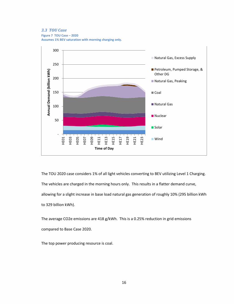
3.3 TOU Case Figure 7 TOU Case – 2020 Assumes 1% BEV saturation with morning charging only.
The TOU 2020 case considers 1% of all light vehicles converting to BEV utilizing Level 1 Charging.
The vehicles are charged in the morning hours only. This results in a flatter demand curve,
allowing for a slight increase in base load natural gas generation of roughly 10% (295 billion kWh
to 329 billion kWh).
The average CO2e emissions are 418 g/kWh. This is a 0.25% reduction in grid emissions
compared to Base Case 2020.
The top power producing resource is coal.
-
50
100
150
200
250
300
HE01
HE03
HE05
HE07
HE09
HE11
HE13
HE15
HE17
HE19
HE21
HE23
Annu
al D
eman
d (b
illio
n kW
h)
Time of Day
Natural Gas, Excess Supply
Petroleum, Pumped Storage, &Other DG
Natural Gas, Peaking
Coal
Natural Gas
Nuclear
Solar
Wind
17
Figure 8 TOU Case – 2030 Assumes 9% BEV saturation with morning charging only.
The TOU Case 2030 shows an expansion of BEVs to 9% of the light vehicle market utilizing Level
1 Charging. These vehicles are all charge at the same times in the morning hours, resulting in a
flatter demand curve. This flat demand curve allows for 304 billion kWh of natural gas
generation to shift to base load, an increase of 57% in base load natural gas generation
compared to Base Case 2030.
The average CO2e emissions are 346.73 g/kWh. This is a 2.17% reduction in grid emissions
compared to Base Case 2030.
The top power producing resource is coal.
-
50
100
150
200
250
300
HE01
HE03
HE05
HE07
HE09
HE11
HE13
HE15
HE17
HE19
HE21
HE23
Annu
al D
eman
d (b
illio
n kW
h)
Time of Day
Natural Gas, Excess Supply
Petroleum, Pumped Storage, &Other DG
Natural Gas, Peaking
Coal
Natural Gas
Nuclear
Solar
Wind
18
Figure 9 TOU Case – 2050 Assumes 52% BEV saturation with continuous charging inverse of normal demand.
The TOU Case 2040 sees further impacts of both a flatter demand curve and renewable
expansion. Additionally, with a significant demand increase from BEVs, new generation is
required to be installed. This new generation is to include all technologies and is considered to
have the average composition of the dispatch model in that given year.
The BEV demand shape is forecasted differently in this model to consider a more continuous
charging structure, as the market penetration at this level would assume a significant BEV
infrastructure buildout.
In this case, natural gas base load now accounts for 81% of natural gas generation and 28% of all
power supplied to the grid, becoming the top generation resource.
The average CO2e emissions are 333 g/kWh. This is a 2.23% reduction in grid emissions
compared to Base Case 2040.
-
50
100
150
200
250
300
HE01
HE03
HE05
HE07
HE09
HE11
HE13
HE15
HE17
HE19
HE21
HE23
Annu
al D
eman
d (b
illio
n kW
h)
Time of Day
New Gen Reqd
Petroleum, Pumped Storage, &Other DG
Natural Gas, Peaking
Coal
Natural Gas
Nuclear
Solar
Wind
19
Figure 10 TOU Case – 2050 Assumes 69% BEV saturation with continuous charging inverse of demand.
The TOU Case 2050 shows further impacts on the demand curve and renewable expansion. The
solar mid-day peak closely tracks the new demand curve, minimizing peak technologies.
As in TOU Case 2040, the BEV demand shape considers a continuous charging scenario.
In this case, natural gas base load now accounts for 94% of natural gas generation and 34% of all
power supplied to the grid, remaining the top generation resource. This amount is double that
of coal, which is a distant second at 17% of power sold.
The average CO2e emissions are 318 g/kWh. This is a 3.45% reduction in grid emissions
compared to Base Case 2050.
-
50
100
150
200
250
300
HE01
HE03
HE05
HE07
HE09
HE11
HE13
HE15
HE17
HE19
HE21
HE23
Annu
al D
eman
d (b
illio
n kW
h)
Time of Day
New Gen Reqd
Petroleum, Pumped Storage, &Other DG
Natural Gas, Peaking
Coal
Natural Gas
Nuclear
Solar
Wind
20
3.4 V2G Case Figure 11 V2G Case – 2020 Assumes 1% BEV saturation, 50% as TOU only and 50% as V2G. Both TOU and V2G assume morning charging and the V2G provides evening dispatch.
The V2G 2020 Case includes a 1% expansion of BEVs, half of which are Level 1 charging identical
to the TOU scenario. The second half are Level 2 charging that export power in the evening,
shown in the chart as Vehicle-To-Grid. It’s important to note that Vehicle-To-Grid technology in
this case does not create power, but shifts power use/supply in time. Since all vehicles, both
TOU and V2G, drive the same distance, they both use the same amount of energy on a net basis.
In this case, due to introduction of V2G, natural gas generation increases further from the TOU
Case and the Base Case, increases of 24% and 39% respectively. This change along with a
reduction of peaking use in the evening creates an emissions profile of 414 g/kWh, a reduction
of 1.37% per kWh compared to Base Case 2020.
The top power producing resource is coal. V2G accounts for 0.43% of all power sold.
-
50
100
150
200
250
300
HE01
HE03
HE05
HE07
HE09
HE11
HE13
HE15
HE17
HE19
HE21
HE23
Annu
al D
eman
d (b
illio
n kW
h)
Time of Day
Natural Gas, Excess Supply
Petroleum, Pumped Storage, &Other DG
Vehicle-To-Grid
Natural Gas, Peaking
Coal
Natural Gas
Nuclear
Solar
Wind
21
Figure 12 V2G Case – 2030 Assumes 9% BEV saturation, 50% as TOU only and 50% as V2G. Both TOU and V2G assume morning charging and the V2G provides evening dispatch.
The V2G 2030 Case shows a further expansion of V2G. However, due to the demand and supply
timing considered in this case, grid efficiency declines. The volatility of natural gas peaking
supply paired with a second peak in the morning for BEV charging compound to reduce the
benefit of BEVs overall.
As a comparison, there is more natural gas base load in the Base 2030 Case than in the V2G
2030 Case. These inefficiencies result in only a slight improvement to grid emissions, a 2.07%
reduction to 347.06 g/kWh. This g/kWh emissions value is higher than the TOU 2030 Case,
indicating that if charging and exporting are contained in the morning and evening only, the grid
is less efficient by allowing V2G technologies.
-
50
100
150
200
250
300HE
01
HE03
HE05
HE07
HE09
HE11
HE13
HE15
HE17
HE19
HE21
HE23
Annu
al D
eman
d (b
illio
n kW
h)
Time of Day
Natural Gas, Excess Supply
Petroleum, Pumped Storage, &Other DG
Vehicle-To-Grid
Natural Gas, Peaking
Coal
Natural Gas
Nuclear
Solar
Wind
22
The top power producing resource is coal. V2G accounts for 3.51% of all power sold.
Figure 13 V2G Case – 2040 Assumes 52% BEV saturation, 50% as TOU only and 50% as V2G. Both TOU and V2G assume continuous charging inverse of standard demand. V2G provides continuous dispatch paired with the aggregate demand curve.
To alleviate the issues caused by strict charging and exporting rules in the V2G 2030 case, the
2040 model assumes a continuous charging and exporting model, as outlined in Appendix A –
Assumptions. The new load curve creates a new mid-day peak. It is important to note that
some vehicles will be charging while others export. V2G now accounts for roughly one quarter
of all like vehicles on the road, resulting in a significant level of BEV dispatched power.
By assuming a more fluid charge/export rule, the load curve is much flatter. In addition, to me
the increased demand, new generation is required. As a result of all these changes, natural gas
increases by 97% compared to Base 2040 Case and 15% compared to TOU 2040 Case.
-
50
100
150
200
250
300HE
01
HE03
HE05
HE07
HE09
HE11
HE13
HE15
HE17
HE19
HE21
HE23
Annu
al D
eman
d (b
illio
n kW
h)
Time of Day
New Gen Reqd
Natural Gas, Excess Supply
Petroleum, Pumped Storage, &Other DG
Vehicle-To-Grid
Natural Gas, Peaking
Coal
Natural Gas
Nuclear
Solar
23
The top power producing resource is base load natural gas. V2G accounts for 15.55% of all
power sold.
Figure 14 V2G Case – 2050 Assumes 69% BEV saturation, 50% as TOU only and 50% as V2G. Both TOU and V2G assume continuous charging inverse of standard demand. V2G provides continuous dispatch paired with the aggregate demand curve.
With a BEVs constituting a large majority of light vehicles on the road, half of which being
capable of exporting power, V2G has effectively shifted the dispatch model. An expanded mid-
day peak remains, as first appeared in the V2G 2040 Case. Base load natural gas shows further
expansion, an increase of 62% compared to Base 2050 Case and 4% compared to TOU 2040
Case.
As in previous cases, new generation is acquired and all associated assumptions are outlined.
The top power producing resource is base load natural gas. V2G accounts for 18.28% of all
power sold, behind only base load natural gas and surpassing coal for the first time.
-
50
100
150
200
250
300
HE01
HE03
HE05
HE07
HE09
HE11
HE13
HE15
HE17
HE19
HE21
HE23
Annu
al D
eman
d (b
illio
n kW
h)
Time of Day
New Gen Reqd
Natural Gas, Excess Supply
Petroleum, Pumped Storage, &Other DG
Vehicle-To-Grid
Natural Gas, Peaking
Coal
Natural Gas
Nuclear
Solar
24
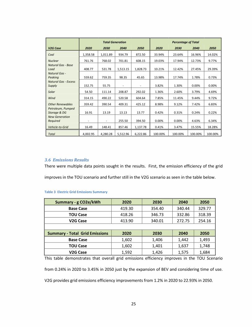
3.5 Generation Resource Summary The following tables summarize the total generation in billion kWh from a given source and the
percentage of that years generation that resource provides.
Total 4,002.95 4,280.28 5,512.96 6,222.86 100.00% 100.00% 100.00% 100.00%
3.6 Emissions Results There were multiple data points sought in the results. First, the emission efficiency of the grid
improves in the TOU scenario and further still in the V2G scenario as seen in the table below.
Table 3 Electric Grid Emissions Summary
Summary - g CO2e/kWh 2020 2030 2040 2050 Base Case 419.30 354.40 340.44 329.77 TOU Case 418.26 346.73 332.86 318.39 V2G Case 413.90 340.01 272.75 254.16
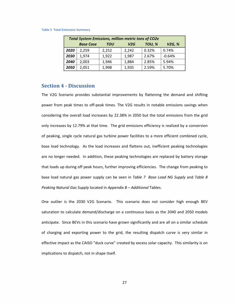
Summary - Total Grid Emissions 2020 2030 2040 2050 Base Case 1,602 1,406 1,442 1,493 TOU Case 1,602 1,401 1,637 1,748 V2G Case 1,592 1,426 1,575 1,684
This table demonstrates that overall grid emissions efficiency improves in the TOU Scenario
from 0.24% in 2020 to 3.45% in 2050 just by the expansion of BEV and considering time of use.
V2G provides grid emissions efficiency improvements from 1.2% in 2020 to 22.93% in 2050.
26
The vehicles individually also achieve better emissions performance when considering the
ultimate fuel source. The assumption that BEVs in general have lower net emissions than a
standard gasoline fueled vehicle was clearly anticipated. The “Base BEV” test assumes the
annual emissions per kWh of the grid and assigns that value to every kWh consumed by a BEV.
The model tested how this can be improved by assuming time of use and vehicle to grid. Those
results are in the table below. The V2G Scenario considers both the emissions of the electricity
consumed and the emissions of the electricity replaced.
Year % of Total BEV Count 2020 1.00% 2,736,130 2030 9.00% 24,625,173 2040 52.00% 142,278,779 2050 69.00% 188,792,995
38
Appendix C - Model Chart Summary
39
Works Cited Bolt EV. (n.d.). Retrieved April 19, 2017, from Chevrolet.com: http://www.chevrolet.com/bolt-
ev-electric-vehicle-2.html?s_tnt=448560%3A1%3A0
CAISO. (2016). What the duck curve tells us about managing green energy. Retrieved April 19, 2017, from California ISO: https://www.caiso.com/Documents/FlexibleResourcesHelpRenewables_FastFacts.pdf
Charging is No Big Deal. (n.d.). Retrieved April 19, 2017, from ChevyEVLife.com: https://www.chevyevlife.com/bolt-ev-charging-guide
Charging on the Road. (n.d.). Retrieved April 19, 2017, from Energy.Gov: https://energy.gov/eere/electricvehicles/charging-road
Dunckley, J. (2016, February 26). Plug-In Electric Vehicle Multi-State Market and Charging Survey. Retrieved April 19, 2017, from EPRI: http://www.epri.com/abstracts/pages/productabstract.aspx?productId=000000003002007495
EIA. (2017, April 10). U.S. Energy-Related CO2 emissions fell 1.7% in 2016. Retrieved April 28, 2017, from US Energy Information Administration: https://www.eia.gov/todayinenergy/detail.php?id=30712
EV Home Charging Station FAQs. (n.d.). Retrieved April 19, 2017, from My Chevrolet Volt: http://www.mychevroletvolt.com/ev-home-charging-station-faqs-is-level-2-240v-charging-worth-it
LeTendre, S., & Denholm, P. (2006, December). Electric & Hybrid Cars: New Load. Fortnightly, pp. 28-37.
Number of vehicles registered in the United States from 1990 to 2015 (in 1,000s). (n.d.). Retrieved April 19, 2017, from Statista: The Statistics Portal: https://www.statista.com/statistics/183505/number-of-vehicles-in-the-united-states-since-1990/
Quality, O. o. (2016, June). Fast Facts: US Transportation Sector Greenhouse Gas Emissions. Retrieved April 19, 2017, from US Environmental Protection Agency: https://nepis.epa.gov/Exe/ZyPDF.cgi?Dockey=P100ONBL.pdf
Saxton, T. (2011, January 31). Understanding Electric Vehicle Charging. Retrieved April 19, 2017, from Plug In America: https://pluginamerica.org/understanding-electric-vehicle-charging/
Wogan, D. (2013, September 12). Running the Numbers on EPA's new CO2 regulations: combined cycle stacks up well. Retrieved April 19, 2017, from Scientific American:
World Nuclear Association. (n.d.). Comparison of Lifecycle Greenhouse Gas Emissions of Various Electricity Generation Sources. Retrieved April 19, 2017, from World-Nuclear.org: http://www.world-nuclear.org/uploadedFiles/org/WNA/Publications/Working_Group_Reports/comparison_of_lifecycle.pdf
Additional Works Cited in the Model Center for Climate and Energy Solutions. (n.d.). Federal Vehicle Standards. Retrieved April 21,
2017, from https://www.c2es.org/federal/executive/vehicle-standards
Electric Reliability Council of Texas (n.d.). Wind Power Production - Hourly Averaged Actual and Forecasted Values. (n.d.). Retrieved April 21, 2017, from http://mis.ercot.com/misapp/GetReports.do?reportTypeId=13028&reportTitle=Wind Power Production - Hourly Averaged Actual and Forecasted Values&showHTMLView=&mimicKey
National Renewable Energy Labratory. (n.d.). PVWatts. Retrieved April 21, 2017, from http://pvwatts.nrel.gov/
PJM. (n.d.). Energy Market. Retrieved April 21, 2017, from http://www.pjm.com/markets-and-operations/energy.aspx
Sassams, L., & Leaton, J. (2017, February). Expect the Unexpected: The Disruptive Power of Low-carbon Technology. Retrieved April 21, 2017, from http://www.carbontracker.org/report/expect-the-unexpected-disruptive-power-low-carbon-technology-solar-electric-vehicles-grantham-imperial/ Produced by Carbon Tracker
U.S. Department of Energy. (n.d.). How can a gallon of gasoline produce 20 pounds of CO2? Retrieved April 21, 2017, from https://www.fueleconomy.gov/feg/contentIncludes/co2_inc.htm
U.S. Energy Information Administration. (2017, January 5). Annual Energy Outlook 2017. Retrieved April 19, 2017, from https://www.eia.gov/outlooks/aeo/
U.S. Energy Information Administration. (n.d.). Average Tested Heat Rates by Prime Mover and Energy Source, 2007-2015. Retrieved April 21, 2017, from https://www.eia.gov/electricity/annual/html/epa_08_02.html
World Nuclear Association (n.d.). Comparison of Lifecycle Greenhouse Gas Emissions by Various Electricity Generation Sources [Scholarly project]. (n.d.). April 19, 2017, from http://www.world-nuclear.org/uploadedFiles/org/WNA/Publications/Working_Group_Reports/comparison_of_lifecycle.pdf
Michael Carite 10201 Pembroke Green Place, Columbia, MD 21044 ● 410-570-1139 ● [email protected]
Summary I am an Energy Finance and Business Development Professional with over 8 years of experience developing over $1 billion in distributed energy projects including solar and CHP. My goal is to find a role that leverages my analytical and forecasting skills in a business development and strategy function. Experience
Touchstone Energy Cooperatives (2016-Current) Director, Business Development Dec 2016 – Current
− Initiated first business development oriented newsletter − Created and hosted webinar content with a focus on policy, technology and market trends − Worked with national energy managers to better manage the cooperative business model − Crafted and started new key account training offerings to members
South Jersey Industries (SJI) (2009-2016)
General Manager, Corporate Development (SJI) Apr 2016 – Dec 2016 − Manage M&A and divestiture processes, including origination, structuring, and execution − Responsible for market research, valuation and executive reporting − Manage preferred supply commodity business with $2M in annual margin
Manager, Business Development & Expansion (SJES) Nov 2013 – Apr 2016 − Closed $7.5MM in margin through unique financial arrangements − Commenced first company social media marketing and SEO campaigns − Closed over 85 MW and $250MM in capital expenditures of renewable energy projects − Participated in local and regional organizations to promote brand in multiple chair roles
Manager, Project Development (Marina Energy) Jun 2011 – Nov 2013 − Closed over 90 MW and $400MM in capital expenditure of photovoltaic projects − Developed, pro formed and financed $55M acquisition of New England based steam loop − Managed construction of $180MM central utility and CHP plant serving a gaming facility
Jr. Manager, Project Development (Marina Energy) Jun 2009 – Jun 2011 − Modeled and closed over 10MW of photovoltaic solar projects worth over $70MM − Evaluated operating efficiencies of multiple facilities throughout energy portfolio − Developed working screening models for CHP, LFGE, and PV opportunities
Education
M.S. Energy Policy & Climate 2015 – 2017 Johns Hopkins University Focus on Renewable Energy Policy Master of Business Administration 2012 - 2014 Villanova University Concentrations in Finance & Strategic Management B.S. Energy Business and Finance 2005 - 2009 Pennsylvania State University Minors in Economics and Italian Language
Certifications & Awards
− Certified Energy Manager (CEM) from Association of Energy Engineers − EMSAGE Laureate Honor, College of Earth & Mineral Sciences, Penn State University