Verified Error Bounds for Isolated Singular Solutions of Polynomial Systems Nan Li and Lihong Zhi KLMM, Academy of Mathematics and Systems Science CAS, Beijing, 100190, China [email protected], [email protected]In this paper, we generalize the algorithm described by Rump and Graillat, as well as our previous work on certifying breadth-one singular solutions of polynomial systems, to compute verified and narrow error bounds such that a slightly perturbed system is guaranteed to possess an isolated singular so- lution within the computed bounds. Our new verification method is based on deflation techniques using smoothing parameters. We demonstrate the per- formance of the algorithm for systems with singular solutions of multiplicity up to hundreds. 1 Introduction It is a challenge problem to solve polynomial systems with singular solutions. In [28], Rall studied some convergence properties of Newton’s method for singular solutions, and many modifications of Newton’s method to restore the quadratic convergence for singular solutions have been proposed in [1, 5, 6, 7, 11, 12, 13, 25, 27, 29, 30, 34, 38]. Recently, some symbolic-numeric methods have also been proposed for refining approximate isolated singular solutions to high accuracy [2, 3, 4, 9, 10, 17, 18, 19, 23, 36, 37]. In [21, 22], we described an algorithm based on the regularized Newton iterations and the computation of differential conditions satisfied at given approximate singular solutions to compute isolated singular solutions accurately to the full machine precision when its Jacobian matrix has corank one (the breadth-one case). Since arbitrary small perturbations of coefficients may transform an iso- lated singular solution into a cluster of simple roots or even make it disappear, it is more difficult to certify that a polynomial system or a nonlinear system 1
Transcript
Verified Error Bounds for Isolated Singular
Solutions of Polynomial Systems
Nan Li and Lihong ZhiKLMM, Academy of Mathematics and Systems Science
In this paper, we generalize the algorithm described by Rump and Graillat,as well as our previous work on certifying breadth-one singular solutions ofpolynomial systems, to compute verified and narrow error bounds such thata slightly perturbed system is guaranteed to possess an isolated singular so-lution within the computed bounds. Our new verification method is based ondeflation techniques using smoothing parameters. We demonstrate the per-formance of the algorithm for systems with singular solutions of multiplicityup to hundreds.
1 Introduction
It is a challenge problem to solve polynomial systems with singular solutions.In [28], Rall studied some convergence properties of Newton’s method forsingular solutions, and many modifications of Newton’s method to restorethe quadratic convergence for singular solutions have been proposed in [1,5, 6, 7, 11, 12, 13, 25, 27, 29, 30, 34, 38]. Recently, some symbolic-numericmethods have also been proposed for refining approximate isolated singularsolutions to high accuracy [2, 3, 4, 9, 10, 17, 18, 19, 23, 36, 37]. In [21, 22], wedescribed an algorithm based on the regularized Newton iterations and thecomputation of differential conditions satisfied at given approximate singularsolutions to compute isolated singular solutions accurately to the full machineprecision when its Jacobian matrix has corank one (the breadth-one case).
Since arbitrary small perturbations of coefficients may transform an iso-lated singular solution into a cluster of simple roots or even make it disappear,it is more difficult to certify that a polynomial system or a nonlinear system
1
has a multiple root, if not the entire computation is performed without anyrounding error.
In [33], by introducing a smoothing parameter, Rump and Graillat de-scribed a verification method for computing guaranteed (real or complex) er-ror bounds such that a slightly perturbed system is proved to have a doubleroot within the computed bounds. In [20], by adding a perturbed univariatepolynomial in one selected variable with some smoothing parameters to oneselected equation of the original system, we generalized the algorithm in [33]to compute guaranteed error bounds, such that a slightly perturbed systemis proved to possess an isolated singular solution whose Jacobian matrix hascorank one within the computed bounds.
In [23], Mantzaflaris and Mourrain proposed a one-step deflation method,and by applying a well-chosen symbolic perturbation, they verified a multipleroot of a nearby system with a given multiplicity structure, which dependson the accuracy of the given approximate singular solution. The size of thedeflated system is equal to the multiplicity times the size of the originalsystem, which might be large (e.g. DZ1 and KSS in Table 1).
In [39], based on deflated square systems proposed by Yamamoto in [38],Kanzawa and Oishi presented a numerical method for proving the existenceof “imperfect singular solutions” of nonlinear equations with guaranteed ac-curacy. In [38], if the second-order deflation is applied, then smoothing pa-rameters are added not only to the original system but also to differentialsystems independently (see (20)). Therefore, one can only prove the exis-tence of an isolated solution of a slightly perturbed system which satisfiesthe first-order differential condition approximately.
In [8, 14, 15], Kearfott et al. presented completely different and extremelyinteresting methods based on verifying a nonzero topological degree to certifythe existence of singular zeros of nonlinear systems.
Main contribution Suppose a polynomial system F and an approximatesingular solution are given. Stimulated by our previous work on certifyingbreadth-one singular solutions [20], we show firstly that the number of de-flations used by Yamamoto to obtain a regular system is bounded by thedepth of the singular solution. Then we show how to move the indepen-dent perturbations in the first-order differential system (20) appeared in [38]back to the original system. We prove that the modified deflations will alsoterminate after a finite number of steps which is bounded by the depth aswell, and return a regular and square augmented system, which can be usedto prove the existence of an isolated singular solution of a slightly perturbedsystem exactly, see Theorem 3.7 and 3.8. Finally, we present an algorithm for
2
computing verified (real or complex) error bounds, such that a slightly per-turbed system is guaranteed to possess an isolated singular solution withinthe computed bounds. The algorithm has been implemented in Maple andMatlab, and narrow error bounds of the order of the relative rounding errorare computed efficiently for examples given in literature.
Structure of the paper Section 2 is devoted to recall some notationsand well-known facts. In Section 3, we present a new deflation methodby adding smoothing parameters properly to the original system, which willreturn a regular and square augmented system within a finite number of stepsbounded by the depth. In Section 4, we propose an algorithm for computingverified (real or complex) error bounds, such that a slightly perturbed systemis guaranteed to possess an isolated singular solution within the computedbounds. Some numerical results are given to demonstrate the performanceof our algorithm in Section 5.
2 Preliminaries
Let F = {f1, . . . , fn} be a polynomial system in C[x] = C[x1, . . . , xn] andI ∈ C[x] be the ideal generated by polynomials in F .
Definition 2.1 An isolated solution of F (x) = 0 is a point x ∈ Cn which
satisfies:
for a small enough ε > 0 : {y ∈ Cn : ‖y − x‖ < ε} ∩ F−1(0) = {x}.
Definition 2.2 We call x a singular solution of F (x) = 0 if and only if
rank(Fx(x)) < n, (1)
where Fx(x) is the Jacobian matrix of F (x) with respect to x.
Definition 2.3 Let Qx be the isolated primary component of the ideal I =(f1, . . . , fn) whose associate prime is mx = (x1 − x1, . . . , xn − xn), then themultiplicity µ of x is defined as µ = dim(C[x]/Qx), and the index ρ of x isdefined as the minimal nonnegative integer ρ such that mρ
x ⊆ Qx [35].
Let dαx : C[x] → C denote the differential functional defined by
dαx(g) =
1
α1! · · ·αn!· ∂|α|g
∂xα11 · · ·∂xαn
n
(x), ∀g(x) ∈ C[x], (2)
for a point x ∈ Cn and an array α ∈ Nn. The normalized differentials havea useful property: when x = 0, we have dα
0(xβ) = 1 if α = β or 0 otherwise.
3
Definition 2.4 The local dual space of I at x is the subspace of elements ofDx = SpanC{dα
x, α ∈ Nn} that vanish on all the elements of I
Dx := {Λ ∈ Dx | Λ(f) = 0, ∀f ∈ I}. (3)
It is clear that dim(Dx) = µ and the maximal degree of an element Λ ∈ Dx
is equal to the index ρ − 1, which is also known as the depth of Dx.A singular solution x of a square system F (x) = 0 satisfies equations
{F (x) = 0,
det(Fx(x)) = 0.(4)
The above augmented system forms the basic idea for the deflation method[25, 26, 27]. But the determinant is usually of high degree, so it is numericallyunstable to evaluate the determinant of the Jacobian matrix.
In [18], Leykin et al. modified (4) by adding new variables and equations.Let r = rank(Fx(x)), then there exists a unique vector λ = (λ1, λ2 . . . , λr+1)
T
such that (x, λ) is an isolated solution of
F (x) = 0,Fx(x)Bλ = 0,
hTλ = 1,
(5)
where B ∈ Cn×(r+1) is a random matrix, h ∈ Cr+1 is a random vector andλ is a vector consisting of r + 1 extra variables λ1, λ2 . . . , λr+1. If (x, λ) isstill a singular solution of (5), the deflation is repeated. Furthermore, theyproved that the number of deflations needed to derive a regular root of anaugmented system is strictly less than the multiplicity of x. Dayton and Zengshowed that the depth of Dx is a tighter bound for the number of deflations[4].
Let IR be the set of real intervals, and IRn and IR
n×n be the set of realinterval vectors and real interval matrices, respectively. Standard verificationmethods for nonlinear systems are based on the following theorem [16, 24, 31].
Theorem 2.5 Let F (x) : Rn → R
n be a polynomial system, and x ∈ Rn.
Given X ∈ IRn with 0 ∈ X and M ∈ IR
n×n satisfies ∇fi(x + X) ⊆ Mi,:, fori = 1, . . . , n. Denote by I the n × n identity matrix and assume
−F−1x (x)F (x) + (I − F−1
x (x)M)X ⊆ int(X). (6)
Then there is a unique x ∈ X with F (x) = 0. Moreover, every matrix M ∈ Mis nonsingular. In particular, the Jacobian matrix Fx(x) is nonsingular.
4
Naturally the non-singularity of the Jacobian matrix Fx(x) restricts the ap-plication of Theorem 2.5 to regular solutions of square systems. Notice thatTheorem 2.5 is valid mutatis mutandis over complex numbers as well. Nextwe will use this theorem to derive a verification method to prove the existenceof an isolated singular solution of a slightly perturbed system.
3 A Square and Regular Augmented System
Let a polynomial system F = {f1, . . . , fn} ∈ C[x] be given and x = (x1, . . . , xn)is an isolated singular solution satisfying F (x) = 0.
The augmented systems (4) and (5) have been used to restore the quadraticconvergence of Newton’s method. But notice that these extended systems arealways over-determined, which are not applicable by Theorem 2.5. Hence, anatural thought of modifications is, whether we could add several smoothingparameters to derive a square system with a nonsingular Jacobian matrix.
In [38], by introducing smoothing parameters, Yamamoto derived squaredeflated systems. These systems were used successfully by Kanzawa andOishi in [39] to certify the existence of “imperfect singular solutions” of poly-nomial systems. However, for isolated singular solutions with high singular-ities, the smoothing parameters are added not only to the original systembut also to differential systems independently (see (20)). Therefore, accord-ing to (21), one can only prove the existence of an isolated solution of aslightly perturbed system which satisfies the first-order differential conditionapproximately.
In the following, we rewrite the deflation techniques in [38] in our setting,and prove that the number of deflations needed to obtain a regular systemis bounded by the depth of Dx, see Theorem 3.2. Then we show how to liftthe independent perturbations in the first-order differential system appearedin (20) back to the original system. We prove that the modified deflationswill terminate after a finite number of steps bounded by the depth of Dx aswell, and return a regular and square augmented system, which can be usedto verify the existence of an isolated singular solution of a slightly perturbedsystem exactly, see Theorem 3.7 and 3.8.
3.1 The first-order deflation
Let x ∈ Cn be an isolated singular solution of F (x) = 0, and
rank(Fx(x)) = n − d, (1 < d ≤ n). (7)
5
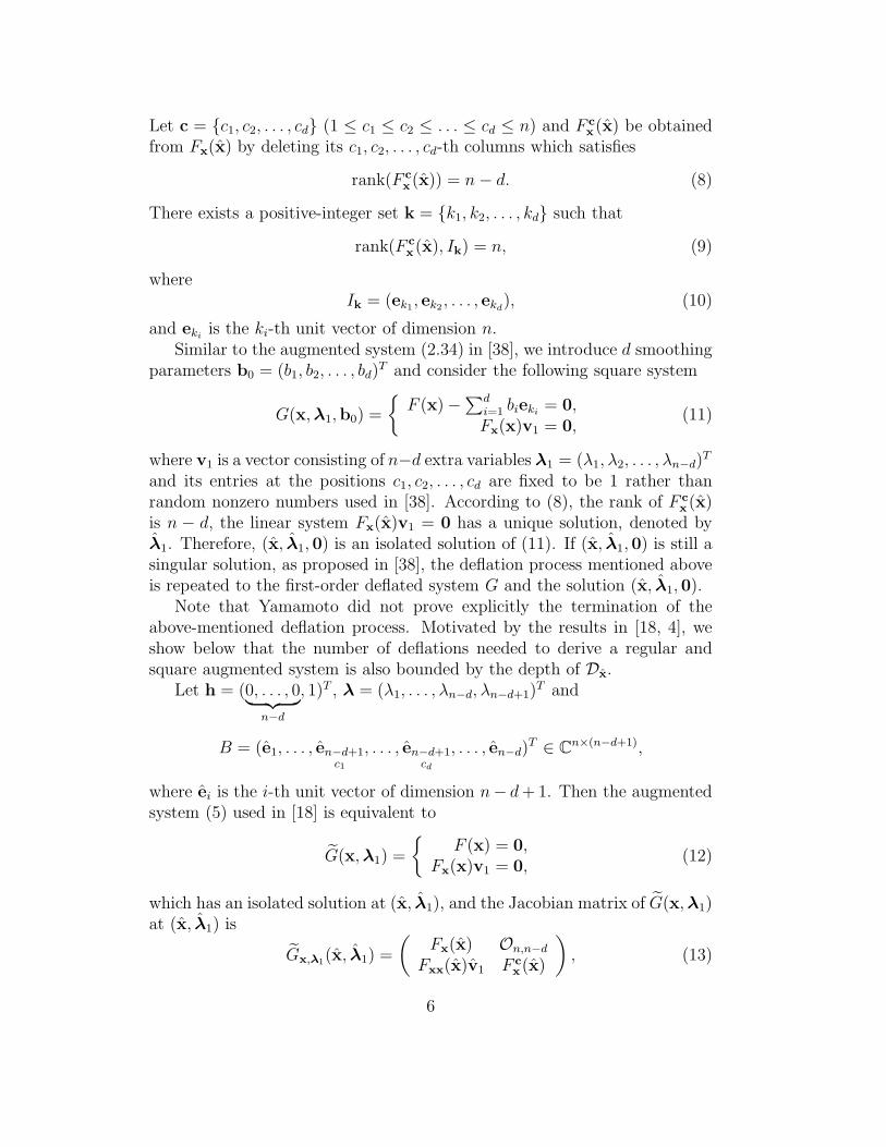
Let c = {c1, c2, . . . , cd} (1 ≤ c1 ≤ c2 ≤ . . . ≤ cd ≤ n) and F cx(x) be obtained
from Fx(x) by deleting its c1, c2, . . . , cd-th columns which satisfies
rank(F cx(x)) = n − d. (8)
There exists a positive-integer set k = {k1, k2, . . . , kd} such that
rank(F cx(x), Ik) = n, (9)
whereIk = (ek1, ek2 , . . . , ekd
), (10)
and ekiis the ki-th unit vector of dimension n.
Similar to the augmented system (2.34) in [38], we introduce d smoothingparameters b0 = (b1, b2, . . . , bd)
T and consider the following square system
G(x, λ1,b0) =
{F (x) − ∑d
i=1 bieki= 0,
Fx(x)v1 = 0,(11)
where v1 is a vector consisting of n−d extra variables λ1 = (λ1, λ2, . . . , λn−d)T
and its entries at the positions c1, c2, . . . , cd are fixed to be 1 rather thanrandom nonzero numbers used in [38]. According to (8), the rank of F c
x(x)is n − d, the linear system Fx(x)v1 = 0 has a unique solution, denoted byλ1. Therefore, (x, λ1, 0) is an isolated solution of (11). If (x, λ1, 0) is still asingular solution, as proposed in [38], the deflation process mentioned aboveis repeated to the first-order deflated system G and the solution (x, λ1, 0).
Note that Yamamoto did not prove explicitly the termination of theabove-mentioned deflation process. Motivated by the results in [18, 4], weshow below that the number of deflations needed to derive a regular andsquare augmented system is also bounded by the depth of Dx.
Let h = (0, . . . , 0︸ ︷︷ ︸n−d
, 1)T , λ = (λ1, . . . , λn−d, λn−d+1)T and
B = (e1, . . . , en−d+1c1
, . . . , en−d+1cd
, . . . , en−d)T ∈ C
n×(n−d+1),
where ei is the i-th unit vector of dimension n− d + 1. Then the augmentedsystem (5) used in [18] is equivalent to
G(x, λ1) =
{F (x) = 0,
Fx(x)v1 = 0,(12)
which has an isolated solution at (x, λ1), and the Jacobian matrix of G(x, λ1)at (x, λ1) is
Gx,λ1(x, λ1) =
(Fx(x) On,n−d
Fxx(x)v1 F cx(x)
), (13)
6
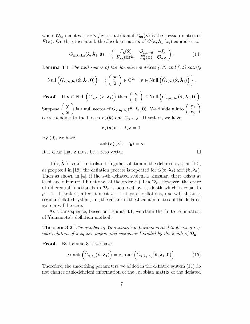
where Oi,j denotes the i× j zero matrix and Fxx(x) is the Hessian matrix ofF (x). On the other hand, the Jacobian matrix of G(x, λ1,b0) computes to
Gx,λ1,b0(x, λ1, 0) =
(Fx(x) On,n−d −Ik
Fxx(x)v1 F cx(x) On,d
). (14)
Lemma 3.1 The null spaces of the Jacobian matrices (13) and (14) satisfy
Null(Gx,λ1,b0(x, λ1, 0)
)=
{(y
0
)∈ C
2n | y ∈ Null(Gx,λ1(x, λ1)
)}.
Proof. If y ∈ Null(Gx,λ1(x, λ1)
)then
(y
0
)∈ Null
(Gx,λ1,b0(x, λ1, 0)
).
Suppose
(y
z
)is a null vector of Gx,λ1,b0(x, λ1, 0). We divide y into
(y1
y2
)
corresponding to the blocks Fx(x) and On,n−d. Therefore, we have
Fx(x)y1 − Ikz = 0.
By (9), we haverank(F c
x(x),−Ik) = n.
It is clear that z must be a zero vector. �
If (x, λ1) is still an isolated singular solution of the deflated system (12),
as proposed in [18], the deflation process is repeated for G(x, λ1) and (x, λ1).Then as shown in [4], if the s-th deflated system is singular, there exists atleast one differential functional of the order s + 1 in Dx. However, the orderof differential functionals in Dx is bounded by its depth which is equal toρ − 1. Therefore, after at most ρ − 1 steps of deflations, one will obtain aregular deflated system, i.e., the corank of the Jacobian matrix of the deflatedsystem will be zero.
As a consequence, based on Lemma 3.1, we claim the finite terminationof Yamamoto’s deflation method.
Theorem 3.2 The number of Yamamoto’s deflations needed to derive a reg-ular solution of a square augmented system is bounded by the depth of Dx.
Proof. By Lemma 3.1, we have
corank(Gx,λ1(x, λ1)
)= corank
(Gx,λ1,b0(x, λ1, 0)
). (15)
Therefore, the smoothing parameters we added in the deflated system (11) donot change rank-deficient information of the Jacobian matrix of the deflated
7
system (12). If corank(Gx,λ1(x, λ1)
)= corank
(Gx,λ1,b0(x, λ1, 0)
)> 0,
then we repeat the deflation steps to (11) and (12) accordingly. Inductively,we know that coranks of Jacobian matrices of two different kinds of deflatedsystems remain equal at every step. Moreover, we have shown that, after asmost ρ − 1 steps, the corank of the Jacobian matrix of the deflated systemcorresponding to (12) will become zero. Therefore, the deflated system cor-responding to (11) will also become regular after at most ρ − 1 steps. �
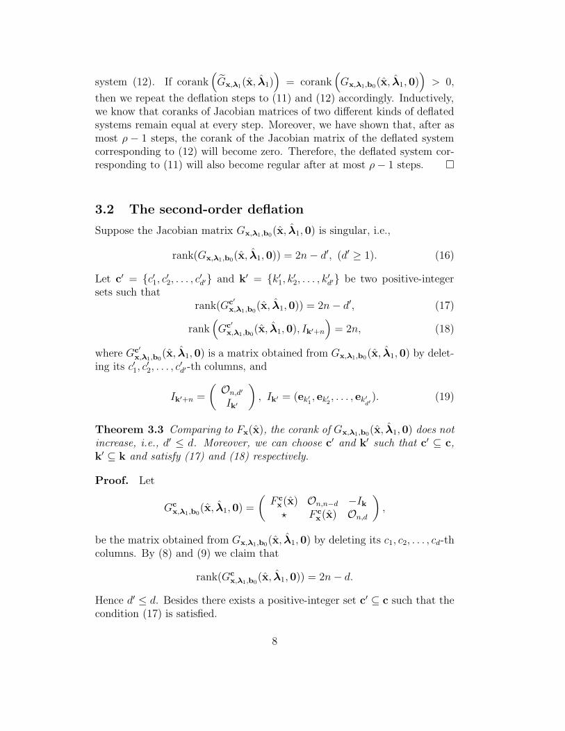
3.2 The second-order deflation
Suppose the Jacobian matrix Gx,λ1,b0(x, λ1, 0) is singular, i.e.,
Let c′ = {c′1, c′2, . . . , c′d′} and k′ = {k′1, k
′2, . . . , k
′d′} be two positive-integer
sets such thatrank(Gc′
x,λ1,b0(x, λ1, 0)) = 2n − d′, (17)
rank(Gc′
x,λ1,b0(x, λ1, 0), Ik′+n
)= 2n, (18)
where Gc′
x,λ1,b0(x, λ1, 0) is a matrix obtained from Gx,λ1,b0(x, λ1, 0) by delet-
ing its c′1, c′2, . . . , c
′d′-th columns, and
Ik′+n =
(On,d′
Ik′
), Ik′ = (ek′
1, ek′
2, . . . , ek′
d′). (19)
Theorem 3.3 Comparing to Fx(x), the corank of Gx,λ1,b0(x, λ1, 0) does notincrease, i.e., d′ ≤ d. Moreover, we can choose c′ and k′ such that c′ ⊆ c,k′ ⊆ k and satisfy (17) and (18) respectively.
Proof. Let
Gcx,λ1,b0
(x, λ1, 0) =
(F c
x(x) On,n−d −Ik
⋆ F cx(x) On,d
),
be the matrix obtained from Gx,λ1,b0(x, λ1, 0) by deleting its c1, c2, . . . , cd-thcolumns. By (8) and (9) we claim that
rank(Gcx,λ1,b0
(x, λ1, 0)) = 2n − d.
Hence d′ ≤ d. Besides there exists a positive-integer set c′ ⊆ c such that thecondition (17) is satisfied.
8
According to (9), it is clear that
rank(Gcx,λ1,b0
(x, λ1, 0), Ik+n) = 2n,
where Ik+n =
(On,d
Ik
). Hence we can choose k′ ⊆ k such that the condition
(18) is satisfied. �
If d′ ≥ 1, then Yamamoto repeated the first-order deflation to G(x, λ1,b0)defined by (11). By Theorem 3.3, we notice that Yamamoto’s second-orderdeflation is equivalent to adding d′ new smoothing parameters denoted by b1
to the first-order differential system Fx(x)v1 = 0, to derive a square system
H(x, λ,b) =
F (x) − Ikb0 = 0,Fx(x)v1 − Ik′b1 = 0,
Gx,λ1,b0(x, λ1,b0)v2 = 0,(20)
where v2 is a vector consisting of 2n−d′ extra variables λ2 and its entries atthe positions c′1, c
′2, . . . , c
′d′ are all 1, and b = (bT
0 ,bT1 )T , λ = (λT
1 , λT2 )T . Let
λ2 denote the unique solution of the linear system Gx,λ1,b0(x, λ1, 0)v2 = 0,
then (x, λ, 0) is an isolated solution of (20).Suppose Theorem 2.5 is applicable to the deflated system H(x, λ,b), and
yields inclusions for x, λ, b0 and b1. Then we have
F (x) = F (x) − Ikb0 = 0 and Fx(x)v1 = Fx(x)v1 = Ik′b1, (21)
where smoothing parameters b1 might be very small, but are not guaranteedto be zeros. Therefore, one can only prove the existence of an isolated solu-tion x of a perturbed system F (x), which satisfies the first-order differentialcondition approximately.
In order to verify the existence of an isolated singular solution of a slightlyperturbed system, we should add the smoothing parameters b1 back to theoriginal system. Let us consider the modified system:
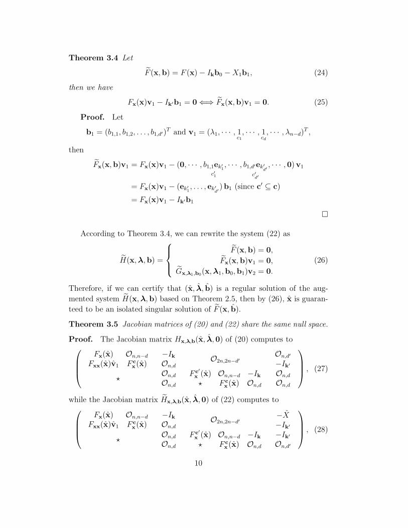
According to Theorem 3.4, we can rewrite the system (22) as
H(x, λ,b) =
F (x,b) = 0,
Fx(x,b)v1 = 0,
Gx,λ1,b0(x, λ1,b0,b1)v2 = 0.
(26)
Therefore, if we can certify that (x, λ, b) is a regular solution of the aug-
mented system H(x, λ,b) based on Theorem 2.5, then by (26), x is guaran-
teed to be an isolated singular solution of F (x, b).
Theorem 3.5 Jacobian matrices of (20) and (22) share the same null space.
Proof. The Jacobian matrix Hx,λ,b(x, λ, 0) of (20) computes to
Fx(x) On,n−d
Fxx(x)v1 F cx(x)
−Ik
On,dO2n,2n−d′
On,d′
−Ik′
⋆On,d
On,d
F c′
x (x) On,n−d −Ik
⋆ F cx(x) On,d
On,d
On,d
, (27)
while the Jacobian matrix Hx,λ,b(x, λ, 0) of (22) computes to
Fx(x) On,n−d
Fxx(x)v1 F cx(x)
−Ik
On,dO2n,2n−d′
−X−Ik′
⋆On,d
On,d
F c′
x (x) On,n−d −Ik
⋆ F cx(x) On,d
−Ik′
On,d′
, (28)
10
where the matrix X consists of vectors xc′(i)ek′(i), i = 1, . . . , d′. Since k′ ⊆ k,we can reduce the last column of the block matrix (28) by its third and sixthcolumns to get the block matrix (27). Therefore, two Jacobian matrices (27)and (28) are of the same corank and share the same null space. �
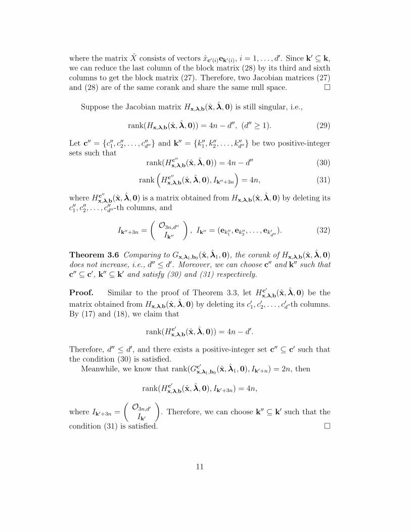
Suppose the Jacobian matrix Hx,λ,b(x, λ, 0) is still singular, i.e.,
rank(Hx,λ,b(x, λ, 0)) = 4n − d′′, (d′′ ≥ 1). (29)
Let c′′ = {c′′1, c′′2, . . . , c′′d′′} and k′′ = {k′′1 , k
′′2 , . . . , k
′′d′′} be two positive-integer
sets such thatrank(Hc′′
x,λ,b(x, λ, 0)) = 4n − d′′ (30)
rank(Hc′′
x,λ,b(x, λ, 0), Ik′′+3n
)= 4n, (31)
where Hc′′
x,λ,b(x, λ, 0) is a matrix obtained from Hx,λ,b(x, λ, 0) by deleting itsc′′1, c
′′2, . . . , c
′′d′′-th columns, and
Ik′′+3n =
(O3n,d′′
Ik′′
), Ik′′ = (ek′′
1, ek′′
2, . . . , ek′
d′′). (32)
Theorem 3.6 Comparing to Gx,λ1,b0(x, λ1, 0), the corank of Hx,λ,b(x, λ, 0)does not increase, i.e., d′′ ≤ d′. Moreover, we can choose c′′ and k′′ such thatc′′ ⊆ c′, k′′ ⊆ k′ and satisfy (30) and (31) respectively.
Proof. Similar to the proof of Theorem 3.3, let Hc′
x,λ,b(x, λ, 0) be the
matrix obtained from Hx,λ,b(x, λ, 0) by deleting its c′1, c′2, . . . , c
′d-th columns.
By (17) and (18), we claim that
rank(Hc′
x,λ,b(x, λ, 0)) = 4n − d′.
Therefore, d′′ ≤ d′, and there exists a positive-integer set c′′ ⊆ c′ such thatthe condition (30) is satisfied.
Meanwhile, we know that rank(Gc′
x,λ1,b0(x, λ1, 0), Ik′+n) = 2n, then
rank(Hc′
x,λ,b(x, λ, 0), Ik′+3n) = 4n,
where Ik′+3n =
(O3n,d′
Ik′
). Therefore, we can choose k′′ ⊆ k′ such that the
condition (31) is satisfied. �
11
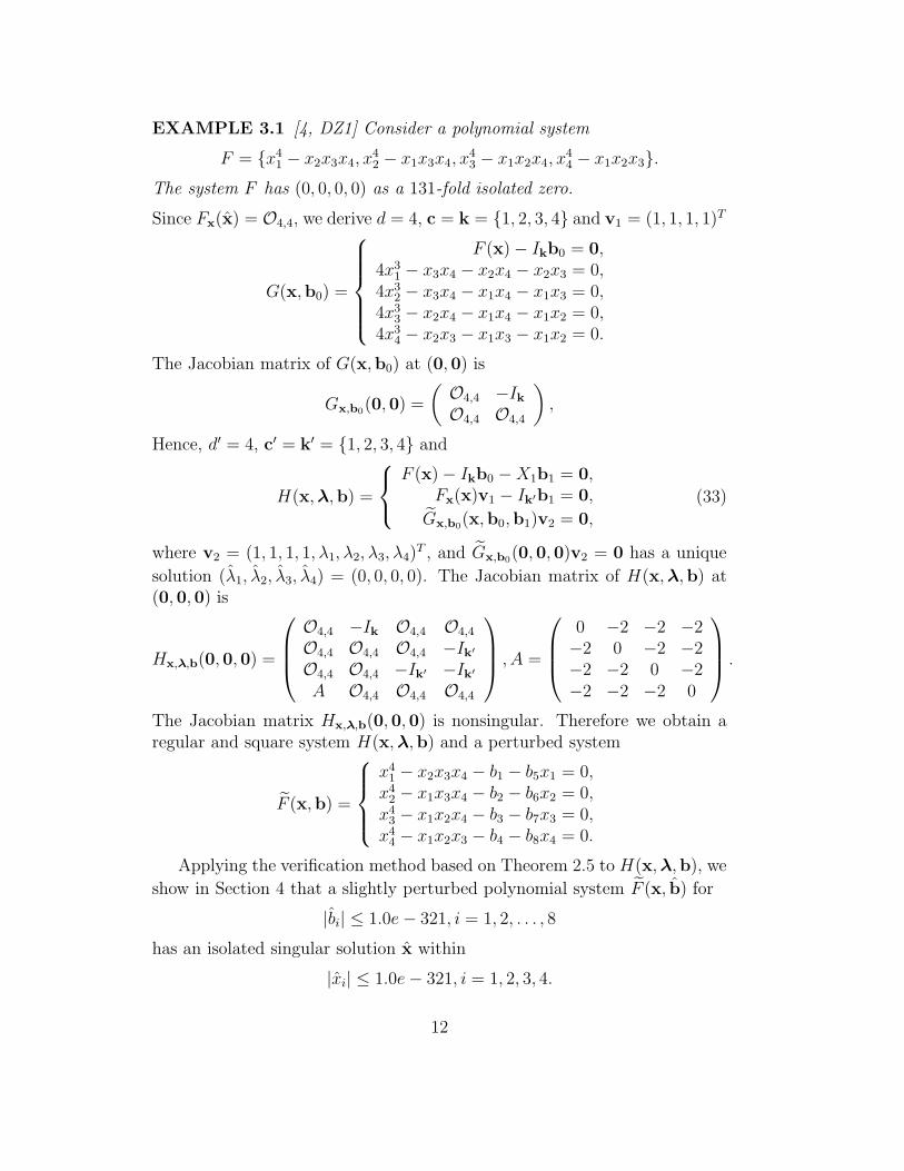
EXAMPLE 3.1 [4, DZ1] Consider a polynomial system
F = {x41 − x2x3x4, x
42 − x1x3x4, x
43 − x1x2x4, x
44 − x1x2x3}.
The system F has (0, 0, 0, 0) as a 131-fold isolated zero.
Since Fx(x) = O4,4, we derive d = 4, c = k = {1, 2, 3, 4} and v1 = (1, 1, 1, 1)T
G(x,b0) =
F (x) − Ikb0 = 0,4x3
1 − x3x4 − x2x4 − x2x3 = 0,4x3
2 − x3x4 − x1x4 − x1x3 = 0,4x3
3 − x2x4 − x1x4 − x1x2 = 0,4x3
4 − x2x3 − x1x3 − x1x2 = 0.
The Jacobian matrix of G(x,b0) at (0, 0) is
Gx,b0(0, 0) =
(O4,4 −Ik
O4,4 O4,4
),
Hence, d′ = 4, c′ = k′ = {1, 2, 3, 4} and
H(x, λ,b) =
F (x) − Ikb0 − X1b1 = 0,Fx(x)v1 − Ik′b1 = 0,
Gx,b0(x,b0,b1)v2 = 0,
(33)
where v2 = (1, 1, 1, 1, λ1, λ2, λ3, λ4)T , and Gx,b0(0, 0, 0)v2 = 0 has a unique
solution (λ1, λ2, λ3, λ4) = (0, 0, 0, 0). The Jacobian matrix of H(x, λ,b) at(0, 0, 0) is
Hx,λ,b(0, 0, 0) =
O4,4 −Ik O4,4 O4,4
O4,4 O4,4 O4,4 −Ik′
O4,4 O4,4 −Ik′ −Ik′
A O4,4 O4,4 O4,4
, A =
0 −2 −2 −2−2 0 −2 −2−2 −2 0 −2−2 −2 −2 0
.
The Jacobian matrix Hx,λ,b(0, 0, 0) is nonsingular. Therefore we obtain aregular and square system H(x, λ,b) and a perturbed system
F (x,b) =
x41 − x2x3x4 − b1 − b5x1 = 0,
x42 − x1x3x4 − b2 − b6x2 = 0,
x43 − x1x2x4 − b3 − b7x3 = 0,
x44 − x1x2x3 − b4 − b8x4 = 0.
Applying the verification method based on Theorem 2.5 to H(x, λ,b), we
show in Section 4 that a slightly perturbed polynomial system F (x, b) for
|bi| ≤ 1.0e − 321, i = 1, 2, . . . , 8
has an isolated singular solution x within
|xi| ≤ 1.0e − 321, i = 1, 2, 3, 4.
12
3.3 Higher-order deflations
For higher-order deflations, in the following, we show inductively how to addnew smoothing parameters properly to the original system in order to derivea square and regular deflated system for certifying the existence of an isolatedsingular solution of a slightly perturbed system.
Let H(0)(x) = F (x), then for the (s + 1)-th deflation, we add smoothingparameters b(s) = (bT
0 , . . . ,bTs )T and consider the following square system
H(s+1)(x, λ(s+1),b(s)) =
F (x,b(s)) = 0,
Fx(x,b(s))v1 = 0,...
G(s)
x,λ(s),b(s−1)(x, λ(s),b(s))vs+1 = 0,
(34)
where λ(s+1) = (λT
1 , . . . , λTs+1)
T are extra variables corresponding to the vec-
tors {v1, . . . ,vs+1}, G(s)(x, λ(s),b(s)) consists of the first 2sn polynomials inH(s+1)(x, λ(s+1),b(s)), and
F (x,b(s)) = F (x) − X0b0 − X1b1 − · · · − Xsbs, (35)
the matrix Xj (0 ≤ j ≤ s) consists of vectors 1j!·xj
c(j)(i)· ek(j)(i), i = 1, . . . , dj,
where c(j) and k(j)are two positive-integer sets selected at the j-th order defla-tion satisfying conditions obtained by replacing the polynomial system F (x)in (8) and (9) by the j-th deflated system H(j)(x, λ(j),b(j−1)) and replacing Ik
by the matrix Ik(j)+(2j−1)n =
(O(2j−1)n,dj
Ik(j)
), Ik(j) = (e
k(j)1
, ek(j)2
, . . . , ek(j)dj
),
where dj is the corank of H(j)
x,λ(j),b(j−1)(x, λ
(j), 0).
Theorem 3.7 The corank ds+1 of H(s+1)
x,λ(s+1),b(s)(x, λ
(s+1), 0) does not increase
and the number of deflations needed to derive a regular solution of an aug-mented system (34) is less than the depth of Dx, i.e., we have
d0 ≥ d1 ≥ · · · ≥ ds+1 ≥ · · · ≥ dρ−1 = 0. (36)
Moreover, we can choose c(j) and k(j) satisfying
c(s) ⊆ · · · ⊆ c(0) and k(s) ⊆ · · · ⊆ k(0). (37)
Proof. Applying Theorem 3.3, 3.5 and 3.6 inductively, we can show thatthe above deflation process (34) produces a decreasing nonnegative-integersequence d0 ≥ d1 ≥ · · · ≥ ds+1 ≥ · · · , which is as same as the sequence
13
consisting of coranks of the Jacobian matrices of the deflated systems by Ya-mamoto’s method. According to Theorem 3.2, the number of Yamamoto’sdeflations to derive a regular solution of an augmented system is bounded bythe depth of Dx. Hence the number of the modified deflations (34) is alsobounded by the depth of Dx. The proof of (37) is similar to the proofs ofTheorem 3.3 and 3.6. �
Theorem 3.8 Suppose Theorem 2.5 is applicable to the augmented system(34), and yields inclusions for x, λ and b. Then the perturbed system F (x, b)has an isolated singular solution at x.
Proof. Since (x, λ, b) is the unique solution of the augmented system (34),we have
F (x, b) = 0 and Fx(x, b)v1 = 0, v1 6= 0.
Hence, x is an isolated singular solution of the slightly perturbed system
F (x, b) = F (x) − X0b0 − X1b1 − · · · − Xsbs.
�
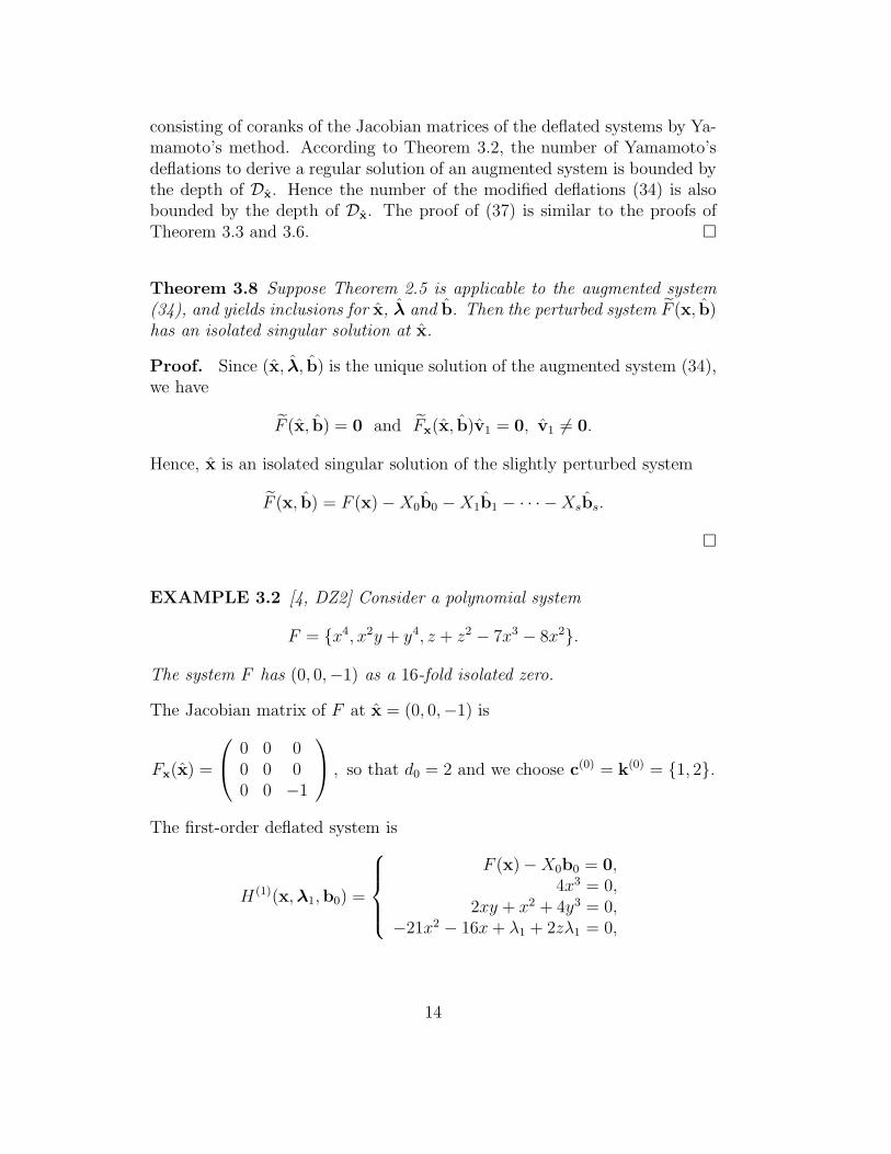
EXAMPLE 3.2 [4, DZ2] Consider a polynomial system
F = {x4, x2y + y4, z + z2 − 7x3 − 8x2}.
The system F has (0, 0,−1) as a 16-fold isolated zero.
The Jacobian matrix of F at x = (0, 0,−1) is
Fx(x) =
0 0 00 0 00 0 −1
, so that d0 = 2 and we choose c(0) = k(0) = {1, 2}.
The first-order deflated system is
H(1)(x, λ1,b0) =
F (x) − X0b0 = 0,4x3 = 0,
2xy + x2 + 4y3 = 0,−21x2 − 16x + λ1 + 2zλ1 = 0,
14
where
X0 = (e1, e2) =
1 00 10 0
, b0 =
(b1
b2
), v1 = (1, 1, λ1)
T , λ1 = (λ1).
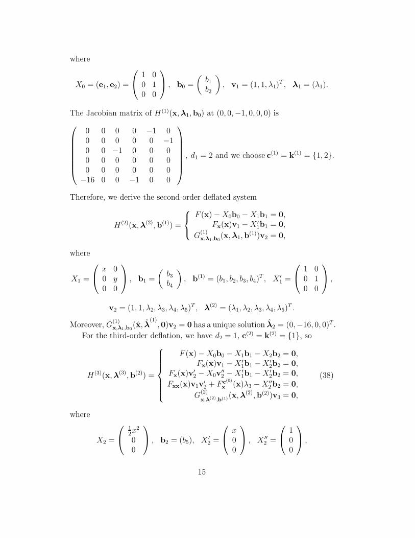
The Jacobian matrix of H(1)(x, λ1,b0) at (0, 0,−1, 0, 0, 0) is
Therefore, we derive the second-order deflated system
H(2)(x, λ(2),b(1)) =
F (x) − X0b0 − X1b1 = 0,Fx(x)v1 − X ′
1b1 = 0,
G(1)x,λ1,b0
(x, λ1,b(1))v2 = 0,
where
X1 =
x 00 y0 0
, b1 =
(b3
b4
), b(1) = (b1, b2, b3, b4)
T , X ′1 =
1 00 10 0
,
v2 = (1, 1, λ2, λ3, λ4, λ5)T , λ
(2) = (λ1, λ2, λ3, λ4, λ5)T .
Moreover, G(1)x,λ1,b0
(x, λ(1)
, 0)v2 = 0 has a unique solution λ2 = (0,−16, 0, 0)T .
For the third-order deflation, we have d2 = 1, c(2) = k(2) = {1}, so
H(3)(x, λ(3),b(2)) =
F (x) − X0b0 − X1b1 − X2b2 = 0,Fx(x)v1 − X ′
1b1 − X ′2b2 = 0,
Fx(x)v′2 − X0v
′′2 − X ′
1b1 − X ′2b2 = 0,
Fxx(x)v1v′2 + F c(0)
x (x)λ3 − X ′′2 b2 = 0,
G(2)
x,λ(2),b(1)(x, λ(2),b(2))v3 = 0,
(38)
where
X2 =
12x2
00
, b2 = (b5), X ′
2 =
x00
, X ′′
2 =
100
,
15
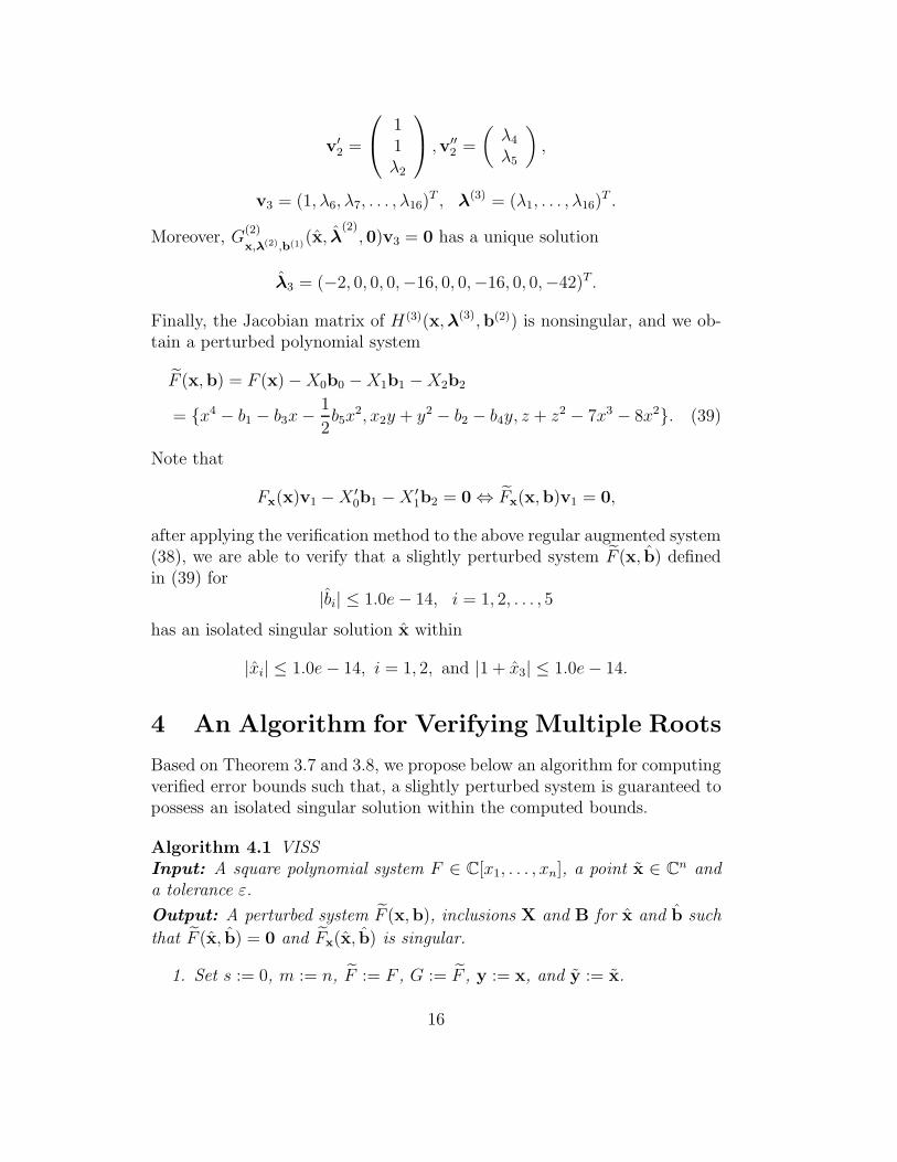
v′2 =
11λ2
,v′′2 =
(λ4
λ5
),
v3 = (1, λ6, λ7, . . . , λ16)T , λ
(3) = (λ1, . . . , λ16)T .
Moreover, G(2)
x,λ(2),b(1)(x, λ
(2), 0)v3 = 0 has a unique solution
λ3 = (−2, 0, 0, 0,−16, 0, 0,−16, 0, 0,−42)T .
Finally, the Jacobian matrix of H(3)(x, λ(3),b(2)) is nonsingular, and we ob-tain a perturbed polynomial system
F (x,b) = F (x) − X0b0 − X1b1 − X2b2
= {x4 − b1 − b3x − 1
2b5x
2, x2y + y2 − b2 − b4y, z + z2 − 7x3 − 8x2}. (39)
Note that
Fx(x)v1 − X ′0b1 − X ′
1b2 = 0 ⇔ Fx(x,b)v1 = 0,
after applying the verification method to the above regular augmented system(38), we are able to verify that a slightly perturbed system F (x, b) definedin (39) for
|bi| ≤ 1.0e − 14, i = 1, 2, . . . , 5
has an isolated singular solution x within
|xi| ≤ 1.0e − 14, i = 1, 2, and |1 + x3| ≤ 1.0e − 14.
4 An Algorithm for Verifying Multiple Roots
Based on Theorem 3.7 and 3.8, we propose below an algorithm for computingverified error bounds such that, a slightly perturbed system is guaranteed topossess an isolated singular solution within the computed bounds.
Algorithm 4.1 VISSInput: A square polynomial system F ∈ C[x1, . . . , xn], a point x ∈ Cn anda tolerance ε.
Output: A perturbed system F (x,b), inclusions X and B for x and b such
that F (x, b) = 0 and Fx(x, b) is singular.
1. Set s := 0, m := n, F := F , G := F , y := x, and y := x.
16
2. Compute d := n− rank(Fx(x), ε), select integer sets c and k satisfying(8) and (9) respectively.
3. Set F := F+Xsbs, where the matrix Xs consists of vectors 1s!·xs
c(i)·ek(i),i = 1, . . . , d.
(a) If s ≥ 1, then set G := F ; for j from 1 to s doG := {G, Gyvj}; y := (y, λj ,bj−1).
(b) Compute y := (y, LeastSquares(Gy(y)vs+1 = 0), 0);
(c) Set G := {G, Gyvs+1}; y := (y, λs+1,bs); m := 2m.
4. Compute d := m − rank(Gy(y), ε);
(a) If d = 0, apply verifynlss to G and y to compute inclusions X
and B for x and b.
(b) Otherwise, select c, k satisfying (8),(9) for the polynomial systemG, set s := s + 1, y = x and go back to Step 3.
Example 3.1 (continued) Given an approximate singular solution x =(.0003445, .0009502, .0003171, .0006948) and a tolerance ε = 0.005, we obtainthe augmented system (33) and a point
After running verifynlss(H, y) in Matlab [32], it yields
−1.0e − 321 ≤ xi ≤ 1.0e − 321, for i = 1, 2, 3, 4,
−1.0e − 321 ≤ bi ≤ 1.0e − 321, for i = 1, 2, . . . , 8.
By Theorem 3.8, this proves that the perturbed polynomial system F (x, b)(|bi| ≤ 1.0e − 321, i = 1, 2, . . . , 8) has an isolated singular solution x within|xi| ≤ 1.0e − 321, i = 1, 2, 3, 4.
Special case The breadth-one case where the corank of the Jacobian ma-trix equals one occurs frequently, and can be treated more efficiently.
In fact, we have shown in [22, Theorem 3.8] that each step of deflationdescribed by (5) only reduces the multiplicity µ of the singular solution x
by 1. According to Theorem 3.7, the number of deflations described by(34) will be µ − 1. Hence, Algorithm VISS generates an augmented regularsystem of the size (2µ−1n)× (2µ−1n). However, in [20], we introduced a moreefficient method based on the parameterized multiplicity structure, to obtain
17
a deflated regular system G(x,b, λ) which is of the size (µn)× (µn) and canbe used to verify not only the existence of an isolated singular solution, butalso its multiplicity structure.
Let us introduce briefly the method in [20] for the special case of breadthone. By adding µ− 1 smoothing parameter b0, b1, . . . , bµ−2 to a well selectedpolynomial, assumed to be f1, we derive a square augmented system
G(x,b, λ) =
F (x,b)
L1(F )...
Lµ−1(F )
= 0, where F (x,b) =
f1(x) − ∑µ−2ν=0
bνxν1
ν!
f2(x)...
fn(x)
,
and L1, . . . , Lµ−1 are parameterized bases of the local dual space in variablesλ. Furthermore, we proved that if Theorem 2.5 is applicable to G and yieldsinclusions for x ∈ R
n, b ∈ Rµ−1 and λ ∈ R
(µ−1)×(n−1) such that G(x, b, λ) =
0, then x is a breadth-one singular solution of F (x, b) = 0 with multiplicityµ and {1, L1, . . . , Lµ−1} with λ = λ is a basis of Dx.
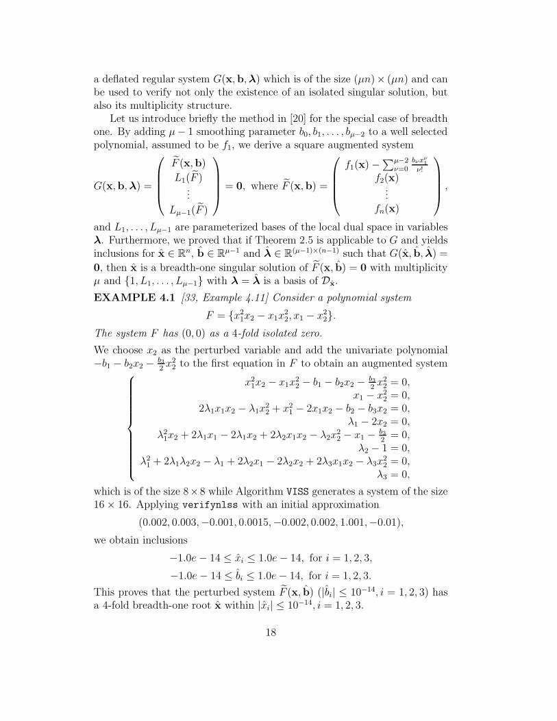
EXAMPLE 4.1 [33, Example 4.11] Consider a polynomial system
F = {x21x2 − x1x
22, x1 − x2
2}.The system F has (0, 0) as a 4-fold isolated zero.
We choose x2 as the perturbed variable and add the univariate polynomial−b1 − b2x2 − b3
2x2
2 to the first equation in F to obtain an augmented system
This proves that the perturbed system F (x, b) (|bi| ≤ 10−14, i = 1, 2, 3) hasa 4-fold breadth-one root x within |xi| ≤ 10−14, i = 1, 2, 3.
18
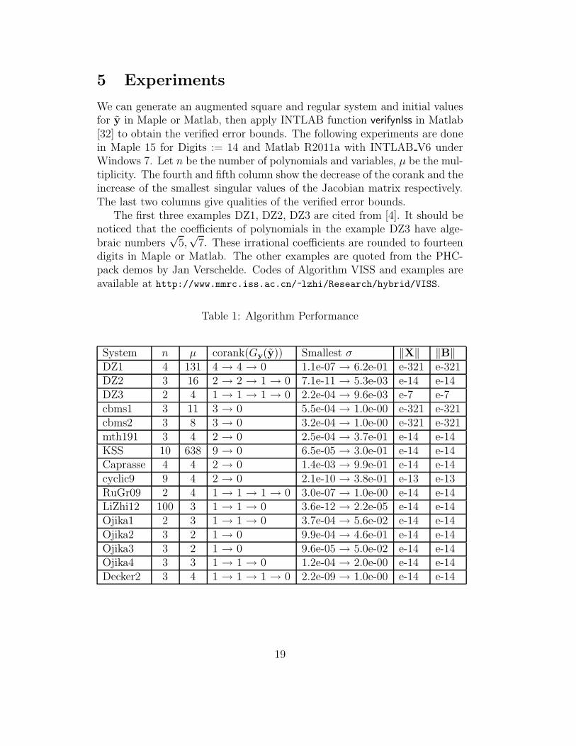
5 Experiments
We can generate an augmented square and regular system and initial valuesfor y in Maple or Matlab, then apply INTLAB function verifynlss in Matlab[32] to obtain the verified error bounds. The following experiments are donein Maple 15 for Digits := 14 and Matlab R2011a with INTLAB V6 underWindows 7. Let n be the number of polynomials and variables, µ be the mul-tiplicity. The fourth and fifth column show the decrease of the corank and theincrease of the smallest singular values of the Jacobian matrix respectively.The last two columns give qualities of the verified error bounds.
The first three examples DZ1, DZ2, DZ3 are cited from [4]. It should benoticed that the coefficients of polynomials in the example DZ3 have alge-braic numbers
√5,√
7. These irrational coefficients are rounded to fourteendigits in Maple or Matlab. The other examples are quoted from the PHC-pack demos by Jan Verschelde. Codes of Algorithm VISS and examples areavailable at http://www.mmrc.iss.ac.cn/~lzhi/Research/hybrid/VISS.
Acknowledgements The authors are grateful to Yijun Zhu for helping usimplement Algorithm VISS in Matlab. The first author is grateful to AntonLeykin for fruitful discussions during the IMA summer program at GeorgiaTech, 2012.
This research is supported by NKBRPC 2011CB302400 and the ChineseNational Natural Science Foundation under Grants: 91118001, 60821002/F02,60911130369 and 10871194.
References
[1] X. Chen, Z. Nashed, and L. Qi, Convergence of Newton’s method forsingular smooth and nonsmooth equations using adaptive outer inverses,SIAM J. on Optimization, 7 (1997), pp. 445–462.
[2] R. Corless, P. Gianni, and B. Trager, A reordered Schur factor-ization method for zero-dimensional polynomial systems with multipleroots, in Proc. 1997 Internat. Symp. Symbolic Algebraic Comput. IS-SAC’97, Kuchlin, ed., New York, 1997, ACM Press, pp. 133–140.
[3] B. Dayton, T. Li, and Z. Zeng, Multiple zeros of nonlinear systems,Mathematics of Computation, 80 (2011), pp. 2143–2168.
[4] B. Dayton and Z. Zeng, Computing the multiplicity structure in solv-ing polynomial systems, in Proceedings of the 2005 international sym-posium on Symbolic and algebraic computation, ISSAC ’05, New York,NY, USA, 2005, ACM, pp. 116–123.
[5] D. W. Decker and C. T. Kelley, Newton’s method at singularpoints. i, SIAM Journal on Numerical Analysis, 17 (1980), pp. 66–70.
[6] , Newton’s method at singular points. ii, SIAM Journal on Numeri-cal Analysis, 17 (1980), pp. 465–471.
[7] , Convergence acceleration for Newton’s method at singular points,SIAM Journal on Numerical Analysis, 19 (1982), pp. 219–229.
[8] J. Dian and R. Kearfott, Existence verification for singular andnonsmooth zeros of real nonlinear systems, Math. Comp, 72 (2003),pp. 757–766.
[9] M. Giusti, G. Lecerf, B. Salvy, and J.-C. Yakoubsohn, Onlocation and approximation of clusters of zeros of analytic functions,Found. Comput. Math., 5 (2005), pp. 257–311.
20
[10] , On location and approximation of clusters of zeros: case of em-bedding dimension one, Found. Comput. Math., 7 (2007), pp. 1–58.
[11] A. Griewank, Analysis and modification of Newton’s method at singu-larities, thesis, Australian National University, 1980.
[12] A. Griewank, On solving nonlinear equations with simple singularitiesor nearly singular solutions, SIAM Review, 27 (1985), pp. 537–563.
[13] A. Griewank and M. R. Osborne, Newton’s method for singularproblems when the dimension of the null space is > 1, SIAM Journal onNumerical Analysis, 18 (1981), pp. 145–149.
[14] R. Kearfott and J. Dian, Existence verification for higher degreesingular zeros of nonlinear systems, SIAM Journal on Numerical Anal-ysis, 41 (2003), pp. 2350–2373.
[15] R. Kearfott, J. Dian, and A. Neumaier, Existence verificationfor singular zeros of complex nonlinear systems, SIAM Journal on Nu-merical Analysis, 38 (2000), pp. 360–379.
[16] R. Krawczyk, Newton-algorithmen zur bestimmung von nullstellen mitfehlerschranken, Computing, (1969), pp. 187–201.
[17] G. Lecerf, Quadratic Newton iteration for systems with multiplicity,Foundations of Computational Mathematics, 2 (2002), pp. 247–293.
[18] A. Leykin, J. Verschelde, and A. Zhao, Newton’s method withdeflation for isolated singularities of polynomial systems, TheoreticalComputer Science, 359 (2006), pp. 111–122.
[19] , Higher-order deflation for polynomial systems with isolated sin-gular solutions, Algorithms in algebraic geometry, 146 IMA Vol. Math.Appl. (2008), pp. 79–97.
[20] N. Li and L. Zhi, Verified error bounds for isolated singular solutionsof polynomial systems: case of breadth one. To appear in TheoreticalComputer Science, DOI: 10.1016/j.tcs.2012.10.028.
[21] , Compute the multiplicity structure of an isolated singular solu-tion: case of breadth one, Journal of Symbolic Computation, 47 (2012),pp. 700–710.
21
[22] , Computing isolated singular solutions of polynomial systems: caseof breadth one, SIAM Journal on Numerical Analysis, 50 (2012), pp. 354–372.
[23] A. Mantzaflaris and B. Mourrain, Deflation and certified iso-lation of singular zeros of polynomial systems, in Proceedings of the36th international symposium on Symbolic and algebraic computation,A. Leykin, ed., ISSAC ’11, New York, NY, USA, 2011, ACM, pp. 249–256.
[24] R. E. Moore, A test for existence of solutions to nonlinear systems,SIAM Journal on Numerical Analysis, 14 (1977), pp. pp. 611–615.
[25] T. Ojika, Modified deflation algorithm for the solution of singular prob-lems, J. Math. Anal. Appl., 123 (1987), pp. 199–221.
[26] , A numerical method for branch points of a system of nonlinear al-gebraic equatuions, Applied Numerical Mathematics, 4 (1988), pp. 419–430.
[27] T. Ojika, S. Watanabe, and T. Mitsui, Deflation algorithm for themultiple roots of a system of nonlinear equations, J. Math. Anal. Appl.,96 (1983), pp. 463–479.
[28] L. Rall, Convergence of the Newton process to multiple solutions, Nu-mer. Math., 9 (1966), pp. 23–37.
[29] G. W. Reddien, On Newton’s method for singular problems, SIAMJournal on Numerical Analysis, 15 (1978), pp. 993–996.
[30] , Newton’s method and high order singularities, Comput. Math.Appl, 5 (1980), pp. 79–86.
[31] S. Rump, Solving algebraic problems with high accuracy, in Proc. of thesymposium on A new approach to scientific computation, San Diego,CA, USA, 1983, Academic Press Professional, Inc., pp. 51–120.
[32] , INTLAB - INTerval LABoratory, in Developments in ReliableComputing, T. Csendes, ed., Kluwer Academic Publishers, Dordrecht,1999, pp. 77–104.
[33] S. Rump and S. Graillat, Verified error bounds for multiple rootsof systems of nonlinear equations, Numerical Algorithms, 54 (2009),pp. 359–377.
22
[34] Y.-Q. Shen and T. J. Ypma, Newton’s method for singular nonlinearequations using approximate left and right nullspaces of the Jacobian,Applied Numerical Mathematics, 54 (2005), pp. 256 – 265. 6th IMACS.
[35] van der Waerden B. L., Algebra, Frederick Ungar Pub. Co., 1970.
[36] X. Wu and L. Zhi, Computing the multiplicity structure from geomet-ric involutive form, in Proc. 2008 Internat. Symp. Symbolic AlgebraicComput. (ISSAC’08), D. Jeffrey, ed., New York, N. Y., 2008, ACMPress, pp. 325–332.
[37] , Determining singular solutions of polynomial systems via symbolic-numeric reduction to geometric involutive forms, Journal of SymbolicComputation, 47 (2012), pp. 227–238.
[38] N. Yamamoto, Regularization of solutions of nonlinear equations withsingular jacobian matrices, Journal of information processing, 7 (1984),pp. 16–21.
[39] K. Yuchi and O. Shin’ichi, Imperfect singular solutions of nonlin-ear equations and a numerical method of proving their existence, IEICEtransactions on fundamentals of electronics, communications and com-puter sciences, 82 (1999), pp. 1062–1069.


![CUSP AREAS OF FAREY MANIFOLDS AND APPLICATIONS TO … · links, butthe metrics they used were singular[5]. For non-singularhyperbolicmetrics, Adams et al. found upper bounds on the](https://static.documents.pub/doc/80x56/5f9260511c7ee7170c69c024/cusp-areas-of-farey-manifolds-and-applications-to-links-butthe-metrics-they-used.jpg)
