INTEGRATED LOTSIZING, SCHEDULING AND BLENDING DECISIONSIN THE SPINNING INDUSTRY
Victor C. B. Camargo1*, Bernardo Almada-Lobo2
and Franklina M. B. Toledo3
Received January 29, 2020 / Accepted March 10, 2021
ABSTRACT. In this paper, the relevance of integrated planning concerning decisions of production andblending in a spinning industry is studied. The scenario regards a plant that produces several yarn packagesover a planning horizon. Each yarn type is produced using a blend of several cotton bales that must containattributes to ensure the quality of the produced yarns. Three approaches to managing production and blend-ing are compared; the first deals with the solution to the production scheduling and blending problems in asingle integrated model. The second approach hierarchically addresses these problems. The third procedurecombines features from the integrated and hierarchical approaches. These approaches are applied to a real-world problem, and their respective performances are analyzed. The third approach proved to deal with lotsizing, scheduling and blending in the spinning industry more efficiently. Moreover, the results indicate theimportance of coordinating production and blending decisions.
Keywords: production planning, lotsizing and scheduling problem, blending problem, spinning industry.
1 INTRODUCTION
The production planning problem in the spinning industry must determine the size and sequenceof yarn production lots as well as which cotton bales will provide a fiber blend that ensures qualityattributes to produce required yarns. These decisions involve lotsizing, scheduling and blendingproblems. The lotsizing and scheduling problem determines the timing, level and sequence ofproduction to meet yarn demand over a time horizon. In order to represent the production en-vironment, constraints related to setup, inventory and capacity must be respected. The blending
*Corresponding author1Departamento de Engenharia de Producao, Universidade Federal de Sao Carlos (UFSCar), Sao Carlos, SP 13565-905,Brazil – E-mail: [email protected] – https://orcid.org/0000-0001-9332-30252INESC TEC, Faculdade de Engenharia, Universidade do Porto, Rua Dr. Roberto Frias s/n, Porto 4200-465, Portugal –E-mail: [email protected] – https://orcid.org/0000-0003-0815-10683Instituto de Ciencias Matematicas e de Computacao, Universidade de Sao Paulo, Caixa Postal 668, Sao Carlos - SP13560-970, Brazil – E-mail: [email protected] – https://orcid.org/0000-0003-2823-7600
2 INTEGRATED LOTSIZING, SCHEDULING AND BLENDING DECISIONS IN THE SPINNING INDUSTRY
problem determines the number of cotton bales used in each blend to feed the spinning machine.These problems arise in a two-stage production system in which the fiber blend is produced at thefirst stage (opening-blending machine) and the yarns are produced at the second stage on variousspinning machines. There is a quality relationship between the first and second stages. The yarnshave attribute specifications that can be achieved by an appropriate blend of fibers (El Mogahzy,2004). The specifications are related to the fiber attributes, such as grade color, trash percentagearea, fiber length and others. Each blend must be composed by a given number of cotton bales inwhich the fibers ensure the specifications of the yarn requirements. The yarns belong to productfamilies that differ in their attributes. Two blend loads for the same yarn family should have aminimal difference regarding their attributes. On contrary, yarns can present different unwantedfeatures, causing production problems at the next level of the textile supply chain. Clearly, theseconstraints show the dependence of the raw cotton blend on the yarn production. Crama et al.(2001) also pointed out the utmost importance of dealing with the raw material in the productionplanning of process industries.
In the past, as pointed out by Hax & Meal (1973), the study of production problems solved hi-erarchically was justified by the data processing incapability of dealing with the optimization ofthe entire system. Planners also used to draw the production plan hierarchically. Even today, hi-erarchical decisions are supported by issues such as a decision-making process involving variouslevels of management and discordant planning horizons. Even though the sequential improve-ment procedures can theoretically converge the hierarchical decisions to an optimum final plan,this approach requires significant computational efforts. Furthermore, some broader objectivescould only be perceived by approaching a detailed integrated model of the production process.This is true in the presence of high interaction among problems, as happens in the spinningindustry dealing with production-scheduling and blending decisions.
The integrated lotsizing and scheduling problem has received attention in the literature due toits relevance to real-world problems. Tackling both problems simultaneously allows for betterproduction plans than those obtained from a hierarchical planning system in which lot sizing isdecided a priori and provides inputs to the scheduling level. Reviews summarizing research onthis subject are presented in Drexl & Kimms (1997), Kallrath (2002), Zhu & Wilhelm (2006),Copil et al. (2017) and Worbelauer et al. (2019). Moreover, some examples of lotsizing andscheduling studies in process industries are those of Kopanos et al. (2010) (yogurt production),Toscano et al. (2019) (beverage industry), Claassen et al. (2016) (food industry) and Camargoet al. (2014) (spinning industry).
In practice, lot sizing and scheduling, and blending in the spinning industry are hierarchicallydetermined. First, lotsizing and scheduling decisions are taken. Then, the blend is defined, loadafter load, to meet the quality specifications. This strategy can be considered myopic, as it doesnot take into account attribute variations in the stored bales that can influence future blendingdecisions, and impact (and constrain) the subsequent plans. In other words, the production plandefined by the traditional hierarchical approach is not executed if the needed set of cotton bales
VICTOR C. B. CAMARGO, BERNARDO ALMADA-LOBO and FRANKLINA M. B. TOLEDO 3
for the blend is not available. Integrating the production-blending problem aims to draw up aproduction plan which has better control concerning attribute variations.
Three approaches to manage these operations are compared in this paper: one in which theproduction-scheduling and blending problems are solved within a single model, another in whichthey are solved separately (in a hierarchical way), and the last is a partial integrated approach.Our integrated model attempts to simultaneously define the production schedule and the selec-tion of cotton bales. In the hierarchical design, the production plan is determined a priori. Then,the cotton bales for each blend load are chosen. Regarding the partial integrated approach, it firstsolves the production schedule, as well as a few blending constraints, and the cotton bales arethen selected in a second step.
This paper aims to show that production planning must contemplate blending constraints in thedecision-making process using mathematical models. This implication is shown by comparingthe production and blending plans given by the integrated and hierarchical approaches. Thiscomparison is built on an instance drawn from a spinning real-world problem. Also, this workprovides three mathematical approaches to assist decision-makers in systemic production andblending planning.
The next section provides a background to the problem appearing in the spinning industry. Theintegrated lot sizing, scheduling and blending is defined in Section 3. The developed integratedmodel is also shown there. An analysis to compare the integrated and hierarchical approaches isreported in Section 4. Section 5 introduces the partial integrated approach that includes featuresfrom the integrated and hierarchical ones. Final remarks and suggestions of future work areaddressed in Section 6.
2 THE SPINNING INDUSTRY
A spinning plant can produce different types of yarns with specifications that are determined bythe customers. Failure to meet yarn specifications causes customer dissatisfaction, a decrease inthe price of the product and a loss of production efficiency. The success of a spinning operationcan be measured by the quality of the produced yarns and the manufacturing costs, and thereforeboth criteria help to determine the competitiveness of a company. The yarn manufacturing costsare measured by the raw material and production process costs. According to Admuthe & Apte(2009), raw material costs can represent up to 70 percent of the yarn price.
In an open-end spinning business, as studied in this paper, raw cotton is purchased in bales. Theproduction flow to transform the raw cotton to yarns is depicted in Figure 1. From beginning toend, the fibers are processed on four machine groups. First, the cotton bales are opened, and thelint blended. The second step is to clean and blend the cotton lint. The third group of machinesaligns and draws the fibers carding to make a long bundle called sliver. Lastly, various spinningmachines draw and twist the sliver to make the yarn. It is wound around bobbins or tubes to betransported to the customers. In this spinning sequence, the two intermediate processes can work
4 INTEGRATED LOTSIZING, SCHEDULING AND BLENDING DECISIONS IN THE SPINNING INDUSTRY
in a synchronized way with the opening and mixing processes. Therefore the production systemconsists of two stages, as illustrated in Figure 1.
Figure 1 – Sequence of processes and stages in yarn production.
The production should be governed by a plan that informs the machine and the time by whicheach required yarn must be produced. While respecting the synchronization of stages, planningmust provide information about the fiber blend, that is, which yarn family is to be producedby each blend load and its starting and finishing times. Once the blend sequence is known, thedecision-maker must select the cotton bales to make up the fiber blend that ensures the specifica-tion for each yarn attribute. A mathematical model to represent this integrated lotsizing, schedul-ing and blending problem is discussed in the next section. Cunha et al. (2018) and Pereira et al.(2020) propose an analysis of decisions related to the raw material by the integration of rawmaterial problems in the lot sizing (and scheduling) problem. However, we propose an approachfocusing on the operational level of decisions.
3 INTEGRATING LOT SIZING, SCHEDULING AND BLENDING
This section proposes a mathematical model for the integrated lotsizing, scheduling and blend-ing problem in the spinning industry. The problem solution draws up a production plan in whichthe blend loads are sequenced, and their required qualities are determined. Moreover, the yarnamount (and its sequence) is established to be produced on each machine complying with theblend quality. The other part of the plan must define the cotton bales selected to be ingredients ofthe blend loads. This planning aims to meet the required specifications for the yarns and shouldminimize production costs and the attribute variability between blends. The mathematical modelpresented below is an integration of the lotsizing and scheduling problem and the blending prob-lem. The lotsizing and scheduling constraints are based on the multi-stage hybrid lotsizing andscheduling model proposed in Camargo et al. (2012). The blending constraints are compatiblewith some ideas from Zago (2005).
3.1 Definition of lotsizing and scheduling problem
A spinning mill can produce different types of yarns on several parallel machines. The productionplan must define the production for each yarn in each period over a finite planning horizon. Thedemand for the yarns is known and should be met when capacity is sufficient. Delays can occurif the demand for yarns is high; therefore, backlogs must be represented in the model.
VICTOR C. B. CAMARGO, BERNARDO ALMADA-LOBO and FRANKLINA M. B. TOLEDO 5
The production of a yarn in a given time period imposes the condition that a suitable fiber blendalso be processed in that bucket. Thus the planning of the second stage requires the planning ofthe first stage. That is, with a blend load (first stage), it is possible to produce specific products(second stage). A blend load consists of a set of bales of a certain quality of fibers. The yarns be-long to families related to the required blend and quality specifications. A fiber blend is generallyused in several yarns, but a yarn is made of only one fiber blend. At each point in time, only onefiber blend can be processed by load on this kind of production line; thus, all the machines mustproduce yarns of the same family. It is possible to produce more than one family, but it requiresthe tracking of raw material and intermediate products. This industrial feature is not consideredin the study.
Machines may differ in their processing rates of the same yarn, and consequently, the fiber blendcan be consumed at different speeds. A setup changeover from one yarn to another consumes acapacity time dependent on the sequence in which the yarns are processed. This characteristicimposes scheduling constraints jointly formulated with lotsizing constraints. Setups can be car-ried from one period to the next. The setup changeover for a fiber blend can be considered nullas another fiber blend is immediately available for later use in production.
The definition of the lotsizing and scheduling problem for the spinning industry can be repre-sented by the following mathematical model, as proposed by Camargo et al. (2014). From theresults shown, this model presented the best results for the problem. The model considers contin-uous time periods for the first stage. In the second stage, production slots are considered, repre-senting production in a semi-continuous manner. The indices, parameters and decision variablesfor the lot sizing and scheduling are defined as follows:
Indicesi = 1, . . . , N yarn types;k = 1, . . . , K yarn families - blend quality types;m = 1, . . . , M spinning machines;t, t ′ = 1, . . . , T periods;l = 1, . . . , L blend loads available within the planning horizon.
Parameterscitt ′ cost of producing one kilogram of yarn i in period t to fulfill the demand of period t ′;σmi j setup cost of a changeover on machine m from yarn i to yarn j;rl cost of one kilogram of residue of the lth blend load;dit ′ demand (kilograms) of yarn i in period t ′;smi j fraction of a single period consumed for the production setup of a changeover on machine m
from yarn i to yarn j;pmi fraction of a single period consumed for production on machine m, of one kilogram of yarn i;C opening-and-blending machine capacity (kilograms) for one blend load;S(k) yarn set belonging to the same family k.
6 INTEGRATED LOTSIZING, SCHEDULING AND BLENDING DECISIONS IN THE SPINNING INDUSTRY
VariablesXmitlt ′ production (kilograms) on machine m of yarn i in period t using the lth blend load to meet
demand in period t ′;Ymi jtl takes 1, if a changeover occurs on machine m from yarn i to j in period t using the lth blend
load; 0 otherwise;Rl raw cotton residue (kilograms) of the lth blend load;Ulk takes 1, if the lth blend load satisfies the quality for yarn family k; 0 otherwise;us
l starting time of the lth blend load;u f
l finishing time of the lth blend load;µs
mitl production starting time on machine m of yarn i in period t using the lth blend load;µ
fmitl production finishing time on machine m of yarn i in period t using the lth blend load;
αmitl takes 1, if machine m is set up for production of yarn i in period t using the lth blend load; 0otherwise;
Pstl takes 1, if the lth blend load starts before the end of period t (that is, instant time t); 0 otherwise;
P ftl takes 1, if the lth blend load ends after the beginning of period t (that is, instant time t−1); 0
VICTOR C. B. CAMARGO, BERNARDO ALMADA-LOBO and FRANKLINA M. B. TOLEDO 7
N
∑j=1
Ym jitl +αmitl =N
∑j=1
Ymi jtl +αmit(l+1) ∀m, i, t, l < L (10)
N
∑j=1
Ym jitL +αmitL =N
∑j=1
Ymi jtL +αmi(t+1)1 ∀m, i, t (11)
N
∑i=1
αmitl = 1 ∀m, t, l (12)
N
∑j=1
Ym jitl ≤ 1 ∀m, i, t, l (13)
M
∑m=1
N
∑i=1
T
∑t=1
T
∑t ′=1
Xmitlt ′ +Rl =C ·K
∑k=1
Ulk ∀l (14)
Xmitlt ′ ≤ dit ′ ·Ulk ∀m, i ∈ S(k)
∀t, l, t ′,k (15)T
∑t=1
N
∑i=1
(µ
fmitl −µ
smitl
)≤ u f
l −usl ∀m, l (16)
µf
mitl −T ·(
Pstl +P f
tl −1)≤ µ
smitl ≤ µ
fmitl +T ·
(Ps
tl +P ftl −1
)∀m, i, t, l (17)
max(t−1;usl −T · (1−Ps
tl))≤ µsmitl ≤ min
(t;u f
l +T ·(
1−P ftl
))∀m, i, t, l (18)
max(t−1;usl −T · (1−Ps
tl))≤ µf
mitl ≤ min(
t;u fl +T ·
(1−P f
tl
))∀m, i, t, l (19)
Ymi jtl ∈ {0,1} ; Ulk ∈ {0,1} ; Pstl ∈ {0,1} ; P f
tl ∈ {0,1} ∀m, i, j, t, l,k (20)
all other variables are non-negative and continuous. (21)
The objective function (1) relates to the lot sizing and scheduling and aims to minimize the costsof backlogging, inventory, changeover and residue. Here, the amount produced before the deliv-ery date is considered as inventory, given by Xmitlt ′ when t < t ′. On the other hand, Xmitlt ′ fort > t ′ is the amount produced after the delivery date, that is, backlogged orders. Similarly, theproduction costs citt ′ refer to holding costs when t < t ′ and to backlog costs when t > t ′. Fort = t ′, citt ′ equals zero, as the production of period t meets the demand of the same period. Notethat to accommodate the unfulfilled demand at the end of the planning horizon, a dummy periodis also considered in the objective function. The constraint group (2)-(4) defines the schedule ofthe blend loads. Each blend load is constrained according to constraints (2) to meet the require-ments for at most one yarn family. Constraints (3) and (4) avoid the overlapping of the startingand finishing blend loads. Note that a blend allocation to a load is allowed without production.Naturally, it generates residues that are detected in the second-stage requirements. Constraints(5)-(13) define the second-stage production system. Equations (5) attempt to satisfy the demandby taking into account inventories and backlogging. Requirements (6) establish the time used toset up the machine and to produce each yarn. Observe that, together with (7), the production slotsare confined to a period of size one. The confinement is made by normalizing Xmitlt ′ with pmi.
Similarly, sm ji refers to the fraction of the period wasted in setting up machine m. Constraints (6)and (7) allow for machine idle times in and between slots. Constraints (8) define the production
8 INTEGRATED LOTSIZING, SCHEDULING AND BLENDING DECISIONS IN THE SPINNING INDUSTRY
slot sequences and avoid sub tour in the sequence. The flow of the machine setup is ensured by(9)-(13). The production is ensured (9) by setting up the machine or carrying a previous config-uration over periods or blends. The setup carried over blend loads and periods is represented in(10) and (11), respectively. Constraints (12) ensure that each machine is set up for the productionof one yarn in each period. Constraints (13) limit one yarn type to changeover to one in eachproduction slot. The constraint group (14)-(19) integrates the first- and second-stage constraints.Constraints (14) define the all-or-nothing production for the blending machine. Specifically, thetotal amount of the blend is used either as production or as residue (Remark (2) presents a casein which the residue must completely used). Requirements (15) allow for yarn production thatbelongs to the family of the blend load in case it exists. Constraints (16)-(19) define the usefulproduction slots, that is, when Ps
tl = P ftl = 1. Let Ps
tl = 1 if the lth blend load starts before theend of period t (i.e. at instant t), Ps
tl = 0 otherwise. Further, P ftl = 1 if the availability of the lth
blend load ends after the beginning of period t (i.e. at instant t− 1), P ftl = 0 otherwise. Figure
2 provides some examples of the variables Pstl and P f
tl . In cases 2.a, 2.b and 2.c, the blend loadstarts before the end of period t (Ps
tl = 1). In cases 2.a, 2.b and 2.d, the blend load finishes afterthe beginning of period t (P f
tl = 1). Constraints (17) are active when Pstl = 0 or P f
tl = 0. In this
t - 1 t t + 1
(a) Pstl = 1; P
ftl = 1
(b) Pstl = 1; P
ftl = 1
(c) Pstl = 1; P
ftl = 0
(d) Pstl = 0; P
ftl = 1
Figure 2 – Illustrative examples for the Ps and P f concept.
case, the lth blend load does not occur in period t and µsmitl = µ
fmitl , forbidding production in that
slot. Constraints (18)-(19) define lower bounds on the production slot starting time, when Pstl = 1,
and upper bounds on the slot ending time, when P ftl = 1.
3.2 Definition of blending problem
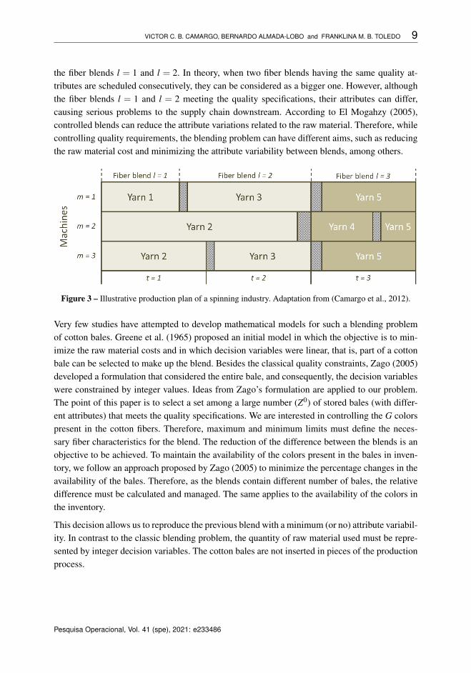
The blending problem is defined by El Mogahzy (2004) and El Mogahzy et al. (2004) as theprocess of combining different fiber attributes to achieve a homogeneous blend. Its importance isemphasized by a fiber statistical analysis in (El Mogahzy, 2004) that testifies the attributes whichaffect the yarn specifications. One of the most common spinning problems that often results fromhigh variability of attributes between blends is the so-called fabric barre. The problem is also de-scribed by the periodic variation in the weft direction, that is, yarns of the same type with slightvariations in an attribute, for example, color can produce a single bicolor piece of cloth. Thisproduct quality issue may be a source of conflict between the spinning and its customers andhighlights the importance of minimizing the variation of quality attributes between two consecu-tive fiber blends. This issue can be seen in Figure 3. Yarn 2 is produced on machine m = 2 using
VICTOR C. B. CAMARGO, BERNARDO ALMADA-LOBO and FRANKLINA M. B. TOLEDO 9
the fiber blends l = 1 and l = 2. In theory, when two fiber blends having the same quality at-tributes are scheduled consecutively, they can be considered as a bigger one. However, althoughthe fiber blends l = 1 and l = 2 meeting the quality specifications, their attributes can differ,causing serious problems to the supply chain downstream. According to El Mogahzy (2005),controlled blends can reduce the attribute variations related to the raw material. Therefore, whilecontrolling quality requirements, the blending problem can have different aims, such as reducingthe raw material cost and minimizing the attribute variability between blends, among others.
Figure 3 – Illustrative production plan of a spinning industry. Adaptation from (Camargo et al., 2012).
Very few studies have attempted to develop mathematical models for such a blending problemof cotton bales. Greene et al. (1965) proposed an initial model in which the objective is to min-imize the raw material costs and in which decision variables were linear, that is, part of a cottonbale can be selected to make up the blend. Besides the classical quality constraints, Zago (2005)developed a formulation that considered the entire bale, and consequently, the decision variableswere constrained by integer values. Ideas from Zago’s formulation are applied to our problem.The point of this paper is to select a set among a large number (Z0) of stored bales (with differ-ent attributes) that meets the quality specifications. We are interested in controlling the G colorspresent in the cotton fibers. Therefore, maximum and minimum limits must define the neces-sary fiber characteristics for the blend. The reduction of the difference between the blends is anobjective to be achieved. To maintain the availability of the colors present in the bales in inven-tory, we follow an approach proposed by Zago (2005) to minimize the percentage changes in theavailability of the bales. Therefore, as the blends contain different number of bales, the relativedifference must be calculated and managed. The same applies to the availability of the colors inthe inventory.
This decision allows us to reproduce the previous blend with a minimum (or no) attribute variabil-ity. In contrast to the classic blending problem, the quantity of raw material used must be repre-sented by integer decision variables. The cotton bales are not inserted in pieces of the productionprocess.
10 INTEGRATED LOTSIZING, SCHEDULING AND BLENDING DECISIONS IN THE SPINNING INDUSTRY
The next model (22)-(32) relates to the blending problem and applies to the cotton bale selectionthat ensures the quality specifications. The additional indices, parameters and decision variablesto be used in this part of the formulation are the following:
Indicesg = 1, . . . , G color grade levels (fiber attribute).
ParametersI0g initial bale inventory level of color grade attribute g;
Z0 total number of bales in the initial inventory;w weight of one cotton bale;q amount of cotton bales for a blend load: q = dC/we;αgk maximum percentage of the color grade attribute g in the blend of type k;
¯αgk minimum percentage of the color grade attribute g in the blend of type k;fgk amount of bales with color grade g used in the last blend load of type k;vgk maximum variation allowed for the color grade attribute g in the blend of type k (in percentage).
Variables
I fg final inventory level of bales with color grade g;
Z f total number of bales in the final inventory;Ag variation (in percentage) of bales with color grade g in the inventory;Hgk variation of bales with color grade g between blends of type k;Dk number of blend loads of type k needed for production;Bk takes 1, if one or more blend loads of type k is used; 0 otherwise;Fgk number of bales with color grade g used in the blend load of type k.
VICTOR C. B. CAMARGO, BERNARDO ALMADA-LOBO and FRANKLINA M. B. TOLEDO 11
Z f = Z0−K
∑k=1
q ·Dk (29)
I fg = I0
g −K
∑k=1
Dk ·Fgk ∀ g (30)
Bk ∈ {0,1} ; Fgk ∈ Z+ ∀ g, k (31)
all other variables are non-negative and continuous. (32)
Objective function targets to minimize the variations of the attributes in the inventory (first sum-mation) and aims to minimize the variations between blends (second summation). λ ′ and λ ′′
allow the decision maker to choose the priority, assigning different weights. Variable Ag holdsthe inventory variation of bales with color grade g, while Hgk holds the variation of bales withcolor grade g between blends of type k. In the following paragraph, we can see an example ofhow variability is calculated. Constraints (23) allocate the variation of the percentage of eachattribute in the inventory using variables Ag. Note that I0
g/Z0 represents the ratio of bales withcolor grade g to the inventory at the beginning of the planning horizon. I f
g /Z f is the ratio of baleswith color grade g to the inventory at the end of the planning horizon. As I f
g and Z f are decisionvariables, constraints (23) are nonlinear. Remark (1) shows an approach to deal with this nonlin-earity. In constraints (24), if one or more blend loads of type k are used (i.e. Dk > 0), Bk takesone. Constraints (25) denote the classical requirements to determine quality limits for attribute gof blend type k. Note that these constraints are active for k such that Bk = 1, that is, only for blendloads used in the planning. Constraints (26) account for the variation of the percentage of eachattribute g between blends that belong to the same type k (yarn family). Constraints (27) limitthe maximum percentage variation of each attribute g between blends to a value predefined bythe decision-maker. The total number of bales in each blend load is accounted by (28), whereasthe total number of bales consumed within the planning horizon is determined by (29). Similarly,equations (30) define the number of stored bales of each attribute at the end of the planning hori-zon. Constraints (31)-(32) enforce the binary, integrality and non-negative requirements for thevariables.
To illustrate the objective function, consider the following example. Suppose that a blend k = 1must be prepared with 150 bales. The initial inventory of bales is I0 = (150,350,750,200,100)with a total Z0 = 1,550 bales. In the previous blend k = 1 the following bales were used:fg1 = (10,40,60,30,10). The variation between blends considers the Fgk values to be usedafter optimization. The variation in the bale inventory includes the remaining I f
g values afterthe use of bales. Thus, if Fg1 = (9,35,63,32,11),
∣∣Fg1− fg1∣∣ = (1,5,3,2,1). Then ∑
Gg=1 Hg1 =
0.08, i.e., there is a 8% variation in the bales between previous and current blends. Simi-
larly, I fg = (141,315,687,168,89) with Z f = 1,400 remaining bales in inventory,
12 INTEGRATED LOTSIZING, SCHEDULING AND BLENDING DECISIONS IN THE SPINNING INDUSTRY
3.3 The integrated formulation
This model incorporates features of the multi-stage hybrid lotsizing and scheduling constraintsfrom Camargo et al. (2012), the simple plant location reformulation Krarup & Bilde (1977) andthe blending constraints from Zago (2005). The problem solution draws up a production planin which the blend loads are sequenced and their required qualities are determined. Moreover,having synchronized quality, the yarn amount (and its sequence) to be produced on each machineis established.
Constraints (33) aim to integrate the lotsizing and scheduling sub-problem - constraints (2)-(21)- with the blending sub-problem - constraints (23)-(32). They count the number of blend loadsof each type k needed to meet the production plan.
Integrating constraints:
Dk =L
∑l=1
Ulk ∀ k (33)
Also, three objective functions are identified during the decision-making process. Specific factorsthat could influence the production-blending decisions ought to be considered jointly. Therefore,the decision-maker can manipulate the weight of each decision. λ represents the influencingweighs of each production-blending decisions in the final objective function (34). However, incase the decision-maker considers λ1 = λ2 = λ3, the terms related to λ2 and λ3 are used onlyas a tiebreaker (due to their magnitudes) between the production plans with the lowest costs ofinventory, backlogging and machine setup.
The integrated lotsizing, scheduling and blending decisions in the spinning model is definedbelow.
Minimize λ1 ·
(M
∑m=1
N
∑i=1
T
∑t=1
L
∑l=1
T
∑t ′=1
citt ′ ·Xmitlt ′ +M
∑m=1
N
∑i=1
N
∑j=1
T
∑t=1
L
∑l=1
σmi j ·Ymi jtl
+L
∑l=1
rl ·Rl
)+λ2 ·
(G
∑g=1
Ag
)+λ3 ·
(K
∑k=1
G
∑g=1
Hgk
) (34)
Subject to:
(2)− (21),
(23)− (33).
The aforementioned model is nonlinear due to requirements (23) and (30). The following remarkshows how such a feature can be tackled. Functions max, min and module can be linearizedstraightforwardly.
VICTOR C. B. CAMARGO, BERNARDO ALMADA-LOBO and FRANKLINA M. B. TOLEDO 13
Remark 1. As Z f , I fg , Dk and Fgk are decision variables, constraints (23) and (30) are nonlinear.
In fact, constraints (29) and (30) are modeled only to define the variables Z f and I fg used in
constraint (23). Given equations (30) and the assumption Z f = Z0−∑Kk=1 q ·Dk, requirements
(23) can be rewritten as
K
∑k=1
Dk ·
∣∣∣∣∣Fgk−q ·I0g
Z0
∣∣∣∣∣= ¯Ag ∀ g, (35)
where ¯Ag denotes the deviation between the planned Fgk and the expected usage of attribute g(see details in Appendix 6).
Let Zk,lk be one, if Dk = l; and 0 otherwise, where lk = 0, . . . , L. That is, the integer number Dk
is codified as a binary summation as follows:
Dk =L
∑lk=0
lk ·Zk,lk ∀ k; (36)
L
∑lk=0
Zk,lk = 1 ∀ k. (37)
Finally, let l1, l2, . . . , lK be indices ∈ {0, . . . , L} and M be a big number, constraints (35) aredefined as:
l1 ·
∣∣∣∣∣Fg1−q ·I0g
Z0
∣∣∣∣∣+ l2 ·
∣∣∣∣∣Fg2−q ·I0g
Z0
∣∣∣∣∣+ . . .+ lK ·
∣∣∣∣∣FgK−q ·I0g
Z0
∣∣∣∣∣≤ ¯Ag +M ·
(K−Z1,l1 −Z2,l2 − . . .−ZK,lK
)∀ g, l1, l2, . . . , lK .
�
K
∑k=1
lk ·
∣∣∣∣∣Fgk−q ·I0g
Z0
∣∣∣∣∣≤ ¯Ag +M ·
(K−
K
∑k=1
Zk,lk
)∀ g, l1, l2, . . . , lK . (38)
�
The mathematical model in this paper considers the raw cotton non-used in the production asresidue (Rl). Some industrial processes do not allow this residue and it must be fully used toproduce yarns. Moreover, without loss of generality, the model takes only into account the colorgrade as the essential attribute to define the yarn quality. Company policies may also considerother attributes as essential. Below, remarks 2 and 3 consider generalizations for the previousformulation: extensions to deal with raw cotton residue and to manage the quality of more thanone fiber attribute.
Remark 2.
We assume in model (1)-(21) that the opening-and-blending machine capacity is completely used.It is represented in constraints (14) by adding a variable Rl to account for the unused cotton. Thecosts of this residue are properly added in the objective function.
14 INTEGRATED LOTSIZING, SCHEDULING AND BLENDING DECISIONS IN THE SPINNING INDUSTRY
Without loss of generality, the residue can also be used for make-to-stock1 production. This speci-ficity can appear in practice. Thus we define XMT S
mitl as the make-to-stock production in machinem of yarn i in period t using the lth blend load. On the other hand, XMTO
mitlt ′ represents the make-to-order production as previously discussed. A couple of constraints should be incorporated toenforce these production cases:
Xmitl = XMT Smitl +
T
∑t ′=1
XMTOmitlt ′ ∀ m, i, t, l; (39)
M
∑m=1
N
∑i=1
T
∑t=1
XMT Smitl = Rl ∀ l. (40)
The total production is used in constraints (39) for make-to-stock and for make-to-order deci-sions. Constraints (40) link the raw material residue to the make-to-stock production. For thisassumption, some constraints must be changed. Constraints (5), (6) and (9) are respectivelyreplaced by
M
∑m=1
T
∑t=1
L
∑l=1
XMTOmitlt ′ = dit ′ ∀i, t ′; (41)
µf
mitl−µsmitl ≥
N
∑j=1
(sm ji ·Ym jitl)+ pmi ·Xmitl ∀m, i, t, l; (42)
pmi ·Xmitl ≤N
∑j=1
Ym jitl +αmitl ∀m, i, t, l. (43)
Constraints (41) ensure that the yarn demand will be fulfilled. Requirements (42) and (43) accom-modate the new production variables Xmitl . Naturally, the objective function has to be updated.�
Remark 3. When more than one fiber attribute must be managed, some constraints and variableshave to be changed in the model, for instance, the company policy required to control the colorgrade (g = 1, . . . ,G) and fiber length (b = 1, . . . ,B) attributes. The inventory level variable isreformulated to incorporate the fiber length attribute (I f
gb) and to inform the number of baleswith color grade g and fiber length b in the inventory at the end of the planning horizon. Similarreformulations are done in variables Fgbk and parameters I0
gb and fgbk. Moreover, variables Ag
and Hgk are specific for the color grade attribute and must be replicated for the fiber length, aswell as the parameters vgk, αgk and
¯αgk. Regarding these assumptions, it is straightforward to
accommodate constraints related to additional attributes in the model. �
1To read more about the combination of make-to-stock and make-to-order production in process industries, see (Somanet al., 2004).
VICTOR C. B. CAMARGO, BERNARDO ALMADA-LOBO and FRANKLINA M. B. TOLEDO 15
3.4 Illustrative example
The usage of the integrated model is illustrated by a small example provided in Tables 1, 2 and 3.The raw material inventory consists of 730 cotton bales. Two types of fiber blends are managedin the example. The inventory and quality limits for the attribute color grade is defined in Table3, as well as the latest blend loads. The maximum variation allowed by the company policies forthe color grade between blends is 7%.
The number of machines is M = 3 and the common resource capacity is C = 20,000 kilos.Machine 1 is set up for product i = 1 at the beginning of the planning horizon and machines 2and 3 are set up for product i = 2. The planning horizon entails T = 3 time periods. Products 1, 2and 3 require the same attributes and belong to product family k = 1, whilst products 4 and 5 arepart of product family k = 2. Inventory (citt ′ |t < t ′) and backlogging costs (citt ′ |t > t ′) are equalfor all periods. Production rates (pmi), setup costs and times (sm ji and σm ji) do not vary betweenmachines.
An optimal lotsizing and scheduling plan is illustrated in Table 4. The most relevant non-zerosolution values for the instance are given. It should be noted that µs
mitl and µf
mitl represent thestarting and finishing times to produce product i on machine m in period t using the lth commonresource batch; Ymi jtl takes on 1, if there is a changeover on machine m from product i to productj in period t, using the lth common resource batch; αmitl equals 1, if the machine m is set upfor product i in the period t using the lth common resource batch; Xmitlt ′ denote the productionvariables. As can be seen, a production plan is determined. The required blend loads are U11 = 1,
Table 5 illustrates the final inventory of cotton bales and the number of bales of each attributedetermined for each blend type. The variation of each color grade is given in percentage.
4 INTEGRATED VS. HIERARCHICAL ANALYSIS
In order to show that the lotsizing and scheduling decisions should not be taken without consider-ing the blending decision jointly, the integrated lotsizing, scheduling and blending model is com-
VICTOR C. B. CAMARGO, BERNARDO ALMADA-LOBO and FRANKLINA M. B. TOLEDO 17
Table 5 – Optimal blending solution to the integrated approach.
Color gradeWhite Light spotted Spotted Tinged
Final inventory (I fg ) 0 200 180 50
Used bales (Fgk) k = 1 85 15 0 0k = 2 60 20 20 0
Variation between blends k = 1 0 0 0.1 0(Hgk) k = 2 0.2 0.7 0.2 0.2
pared to the hierarchical approach. The integrated model can be decoupled into a lotsizing andscheduling sub-model and a blending sub-model by ignoring constraints (33): Dk =∑
Ll=1 Ulk, ∀ k.
Figure 4 illustrates the steps for a hierarchical solution to the problem.
Figure 4 – Step flow for hierarchical production-scheduling and blending.
First, this hierarchical approach determines the lot sizing and scheduling. From the sequenceof the blends, one can implicitly obtain the number of blends of each type needed to carry outthe production, that is, Dk is the input data for the blending definition. Thus the blending solu-tion gives the set of bales that satisfy the quality specifications for the yarns. The lotsizing andscheduling formulation reads as follows:
Lot sizing and scheduling:
Minimize
λ1 ·
(M
∑m=1
N
∑i=1
T
∑t=1
L
∑l=1
T
∑t ′=1
citt ′ ·Xmitlt ′ +M
∑m=1
N
∑i=1
N
∑j=1
T
∑t=1
L
∑l=1
σmi j ·Ymi jtl
+L
∑l=1
rl ·Rl
)
Subject to:
(2)− (19)
Ymi jtl ∈ {0,1} ; Ulk ∈ {0,1} ; Pstl ∈ {0,1} ; P f
tl ∈ {0,1} ∀m, i, j, t, l,k
all other variables are non-negative and continuous.
18 INTEGRATED LOTSIZING, SCHEDULING AND BLENDING DECISIONS IN THE SPINNING INDUSTRY
Blending:
Minimize λ2 ·
(G
∑g=1
Ag
)+λ3 ·
(K
∑k=1
G
∑g=1
Hgk
)
Subject to:
(23)− (30)
Bk ∈ {0,1} ; Fgk ∈ Z+ ∀ g, k
all other variables are non-negative and continuous.
4.1 Sensitivity analysis
The integrated and hierarchical approaches can be compared by applying both to a specific setof data based on a real-world problem, in which the raw material inventory consists of 3,847cotton bales. Company policy considers four attributes as crucial in terms of defining the blend:supplier, color, leaf grade, and short fiber index (SFI), respectively, with 18, 3, 2 and 2 differentpossible values. All costs are derived from the opportunity cost per yarn package unit. Otherparameters related to the production environment (e.g., setup and processing times and machinecapacities) are derived or similar to the real data. The number of yarns N is five and they belongto two product families K.
Moreover, K is the number of different types of blends. The number of spinning machines Mis three. The number of periods T is equal to five, and the maximum number of blend load inthe planning horizon L is fixed at six. The opening-blending machine has the capacity set to 100bales of 200 kilograms each. Demands for yarns are obtained from an order book of the spinningmill. The complete instance is available on GitHub.
The models were generated in OPL language and solved by the CPLEX mixed-integer solverversion 12.10. Tests were conducted on an Intel computer at 2.7 GHz with 16 GB of RAM. Therunning time was limited to 10 minutes for each test. In all tests, the optimal solution was foundwithin the time limit.
Figure 5 depicts the behavior of the integrated and hierarchical approaches to find feasible plansunder an upper bound to the variability between blends (VBB). VBB means vgk in the mathemat-ical formulation. Figure 6 shows the variability of the attributes in the inventory, considering thelimitation to VBB given by the production plans of both integrated and hierarchical approaches.Several values to VBB were checked. A comparison of the integrated and hierarchical approachesrelies on the unfulfilled demand and the variation of the attributes in the inventory. Figures 5 and6 must be analyzed together. As can be seen in Figure 5, regardless of the VBB limit, unfulfilleddemand given by the hierarchical approach is constant. The production plan is defined at the firststep (lotsizing and scheduling problem) and does not consider any information about the blend-ing requirements; that is, the blend sequence is given in the production plan without informationif it is possible to ensure its quality. For VBB limits greater than 0.07, the results of the integrated
VICTOR C. B. CAMARGO, BERNARDO ALMADA-LOBO and FRANKLINA M. B. TOLEDO 19
model resemble those from the hierarchical approach. On the other hand, the integrated approachfinds solutions with higher production costs for VBB limited to 0.07 or less. By looking at thevariation of the attributes in the inventory (Figure 6), the hierarchical approach is not able to findsolutions at the blending step when the VBB is limited to 0.07 or less.
When company policies require yarn production with hard quality constraints, the hierarchicalapproach corresponds to a trial and error approach. When D′k provides an unfeasible solution, anew lotsizing and scheduling solution is requested with an additional constraint to avoid D′k. Inpractice, the hierarchical approach may require several iterations between the problems to delivera production plan with blending constraints satisfied. In some cases, feasible solutions could notbe found. However, the integrated approach delivers the optimal Dk concerning the strict qualityconstraints. Blending requirements are met waiving the best production decision. This fact canbe seen in Figure 5, where high unfulfilled demand represents the backorder.
0.00 0.05 0.10 0.15 0.200.2
0.3
0.4
0.5
Unf
ulfil
led
dem
and
(%)
Limitation of the variability between blends (VBB) (%)
Integrated approach Hierarchical approach: infeasible information to the blending problem Hierarchical approach: feasible information to the blending problem
Figure 5 – Integrated versus hierarchical approach - production cost behavior.
As one can see in Figure 6, the hierarchical approach delivers blends without variation of theattributes in the inventory if Dk is feasible. The integrated approach should also deliver blendswithout variation. However, the values reported by the integrated approach can be explainedby blending decisions having low weight (λ2 and λ3) in the objective function. Decisions ofa lower weight are used as tiebreakers for solutions with similar decisions of a higher weight(λ1). However, lower weight decisions have little influence on the absolute value of the objectivefunction (and, consequently, on the optimality gap).
It is worth noting in Figure 6 that the hierarchical approach delivers blends without variationof the attributes in the inventory. It happens because the cotton inventory has enough quality to
20 INTEGRATED LOTSIZING, SCHEDULING AND BLENDING DECISIONS IN THE SPINNING INDUSTRY
Figure 6 – Integrated versus hierarchical approach - attribute variability in the inventory.
ensure minimal variation between blends VBB less than 0.07 without variation of the attributesin the inventory. Then in case VBB is limited to 0.08, solutions are dominated. It is possibleto easily obtain the minimum VBB admitted by inventory to fulfill the yarn demand. It is alsoclear that variations of attributes in the inventory increase when limitation on variability betweenblends (VBB) decreases.
Consequently, the best of both worlds - the combined integrated and hierarchical approaches -can better achieve the objectives defined for integrated lot sizing, scheduling and blending.
5 PARTIAL INTEGRATED APPROACH FOR PRODUCTION SCHEDULING ANDBLENDING DECISIONS
The partial integrated approach for coordinating production and blending planning attempts tocombine features from those above integrated and hierarchical approaches. The aim is to pro-vide the lotsizing and scheduling problem with blending constraints to foster production planshaving strict quality requirements. On the other hand, specific decisions for minimizing attributevariation can be found by the blending model without the optimality gap hurdle of the integratedapproach. The partial integrated approach for production scheduling and blending is written asfollows:
VICTOR C. B. CAMARGO, BERNARDO ALMADA-LOBO and FRANKLINA M. B. TOLEDO 21
Subject to
Lotsizing and scheduling constraints: (2)− (19)
Some blending constraints: (24)− (28)
Bk ∈ {0,1} ; Fgk ∈ Z+ ∀ g, k
Ymi jtl ∈ {0,1} ; Ulk ∈ {0,1} ; Pstl ∈ {0,1} ; P f
tl ∈ {0,1}∀m, i, j, t, l,k
all other variables are non-negative and continuous.
As can be observed, the partial integrated production and blending planning takes into accountsome of the blending requirements. Minimal variations between blends are ensured, but thoserelated to attribute variation in the inventory are skipped. In the same way as in the hierarchicalapproach, the blending sequence (∑L
l=1 Ulk = Dk) defines the input data for the blending model.However, unlike the hierarchical case, the partial integrated approach provides feasible parame-ters Dk. Thus the blending solution can give the set of bales that fulfills the quality specificationsas the feasibility is tested in advance. Note that the blending model is the same as that of thehierarchical approach (see Section 4).
Remark 4. In the partial integrated approach, some blending constraints (24) - (28) are appliedto both lotsizing and scheduling problem and blending problem. This strategy enforces the lot-sizing and scheduling formulation to deliver a feasible plan of blend loads. On the other hand,those constraints can not be omitted in the blending model else, the variability between blends isnot taken into account in the bale selection. �
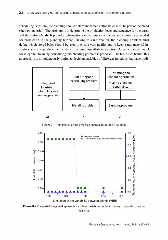
Figure 7 compares the different proposed approaches. The integrated approach (7a) solves theproblem in a single process while the hierarchical approach (7b) firstly deals with the lotsizingand scheduling problem and determines the blending decisions afterward. The partial integratedapproach (7c) solves the lotsizing and scheduling problem considering some blending constraintsto find a feasible production plan to the blending problem subsequently solved.
The partial integrated approach is also analyzed in Figure 8, which depicts both the unfulfilleddemand and the variation of the attributes in the inventory. Note that the green squares refer tounfulfilled demand and the blue triangles to the total variability of the attributes in the inventory.
From these results, the partial integrated approach can determine feasible production plans hav-ing strict quality specifications and can define the best set of cotton bales. As can be seen, theunfulfilled demand resembles that delivered by the integrated approach and the attribute varia-tion caused in the inventory is optimal, which is similar to the single blending problem (compareFigure 8 against Figures 5 and 6).
6 CONCLUSION
In this paper, we have discussed the importance of integrating the production and blending plan-ning problems dealing with attribute variability constraints. Besides the traditional lotsizing and
22 INTEGRATED LOTSIZING, SCHEDULING AND BLENDING DECISIONS IN THE SPINNING INDUSTRY
scheduling decisions, the planning should determine which cotton bales must be part of the blend(the raw material). The problem is to determine the production level and sequence for the yarnsand the cotton blends. It provides information on the number of blends and cotton bales neededfor production in the planning horizon. Having this information, the blending problem mustdefine which stored bales should be used to ensure yarn quality and to keep a raw material in-ventory able to reproduce the blends with a minimum attribute variation. A mathematical modelfor integrated lotsizing, scheduling and blending problem is proposed. The basic idea behind thisapproach is to simultaneously optimize decision variables of different functions that have tradi-
Figure 7 – Comparison of the proposed approaches to find a solution.
0.00 0.05 0.10 0.15 0.20
0.25
0.30
0.35
0.40
0.45
0.50
0.55
Unfulfilled demand Total variability of the attributes in the inventory
Limitation of the variability between blends (VBB)
Unf
ulfil
led
dem
and
(%)
0.0
0.2
0.4
0.6
0.8
1.0 Total variability of the attributes in the inventory
Figure 8 – The partial integrated approach - attribute variability in the inventory and production costbehavior.
VICTOR C. B. CAMARGO, BERNARDO ALMADA-LOBO and FRANKLINA M. B. TOLEDO 23
tionally been optimized sequentially. The hierarchical approach is proposed so that the lotsizingand scheduling problem is solved a priori. Then, the blending problem defines the set of cottonbales that meets the quality requirements.
The integrated model and the hierarchical approach are compared, and from the results, we notethe influence of the raw material inventory on lotsizing and scheduling decisions. The analysisof the results indicates that a feasible production plan can only be obtained if blending relatedconstraints are taken into account. When the product quality has to be controlled, it is reasonableto suggest the integration of lotsizing, scheduling and blending decisions. Moreover, the partialintegrated approach is a purpose that incorporates some blending constraints to ensure the yarnquality when planning the production in the first phase. In addition, the partial approach hasthe accuracy of the blending phase to find the set of cotton bales with minimal variations in theinventory and between blends.
In conclusion, production planning without taking into account raw material requirements canoften be a source of production problems. It can generate impractical plans or cause customerdissatisfaction and a decrease in the price of the product in case of not complying with yarnspecifications. We believe our study has shown that, considering the restricted quality conditions,coordinating production and blending can be extremely important.
Further research towards multi-objective decisions can assist the decision-maker to define a pro-duction plan and choose cotton blends with the best trade-off between the attribute variabilityand production costs. A set of experiments should indicate the strengths and advantages of eachof the mathematical models, in terms of the quality of the solutions provided and the compu-tational burden to solve them. Moreover, the analysis of the integrated problem might help thepurchasing department on how to define the orders for cotton bales and the sales department onwhich yarn type can be produced and sold. The purchase can also be oriented by the productionplan to keep the attribute variability in the inventory and to indirectly maximize the reproductionof blends. Other industries (such as coffee, emulsified meat, pulp and paper, etc.) may benefitfrom the production planning approaches developed in this paper. In this direction, the develop-ment of an advanced planning and scheduling system (APS) that covers the production planningfunctionality for these types of industries can follow the framework proposed in Fachini et al.(2018).
References
[1] ADMUTHE LS & APTE SD. 2009. Optimization of spinning process using hybrid ap-proach involving ANN, GA and linear programming. Proceedings of the 2nd BangaloreAnnual Compute Conference, pp. 1–4.
[2] CAMARGO VCB, TOLEDO FMB & ALMADA-LOBO B. 2012. Three time-based scaleformulations for the two-stage lot sizing and scheduling in process industries. Journal ofthe Operational Research Society, 63: 1613–1630.
24 INTEGRATED LOTSIZING, SCHEDULING AND BLENDING DECISIONS IN THE SPINNING INDUSTRY
[3] CAMARGO VCB, TOLEDO FMB & ALMADA-LOBO B. 2014. HOPS - Hamming-Oriented Partition Search for production planning in the spinning industry. EuropeanJournal of Operational Research, 234(1): 266–277.
[4] CLAASSEN G, GERDESSEN JC, HENDRIX EM & VAN DER VORST JG. 2016. On pro-duction planning and scheduling in food processing industry: Modelling non-triangularsetups andproduct decay. Computers & Operations Research, 76: 147–154.
[5] COPIL K, WORBELAUER M, MEYR H & TEMPELMEIER H. 2017. Simultaneous lotsiz-ing and scheduling problems: a classification and review of models. OR spectrum, 39(1):1–64.
[6] CRAMA Y, POCHET Y & WERA Y. 2001. A discussion of production planningapproaches in the process industry. CORE Discussion Papers 2001042. Universitecatholique de Louvain, Center for Operations Research and Econometrics (CORE).
[7] CUNHA AL, SANTOS MO, MORABITO R & BARBOSA-POVOA A. 2018. An integratedapproach for production lot sizing and raw material purchasing. European Journal ofOperational Research, 269: 923–938.
[8] DREXL A & KIMMS A. 1997. Lot sizing and scheduling - Survey and extensions.European Journal of Operational Research, 99: 221–235.
[9] EL MOGAHZY Y. 2004. An Integrated Approach to Analyzing the Nature of Multi-component Fiber Blending - Part I: Analytical Aspects. Textile Research Journal, 78:701–712.
[10] EL MOGAHZY Y. 2005. Specific approaches for cutting manufacturing cost andincreasing profitability using the EFS system. In: EFS System Conference Presentations.
[11] EL MOGAHZY Y, FARAG R, ABDELHADY F & MOHAMED A. 2004. An Integrated Ap-proach to Analyzing the Nature of Multicomponent Fiber Blending - Part II: ExperimentalAnalysis of Structural and Attributive Blending. Textile Research Journal, 74: 767–775.
[12] FACHINI RF, ESPOSTO KF & CAMARGO VCB. 2018. A framework for development ofadvanced planning and scheduling (APS) systems in glass container industry. Journal ofManufacturing Technology Management, 29: 570–587.
[13] GREENE JH, CHATTO K, HICKS CR, COX CB, BAYNHAM TE & BAYNAM TEJ. 1965.Linear programming - Cotton blending and production allocation. Tech. rep.. InternationalBusiness Machines Corporation (IBM); The Journal of Industrial Engineering.
[14] HAX AC & MEAL HC. 1973. Hierarchical integration of production planning andscheduling. Working papers 656-673. Massachusetts Institute of Technology (MIT),Sloan School of Management.
VICTOR C. B. CAMARGO, BERNARDO ALMADA-LOBO and FRANKLINA M. B. TOLEDO 25
[15] KALLRATH J. 2002. Planning and scheduling in the process industry. OR Spectrum, 24:219–250.
[16] KOPANOS GM, PUIGJANER L & GEORGIADIS MC. 2010. Optimal production schedul-ing and lot-sizing in dairy plants: the yogurt production line. Industrial & EngineeringChemistry Research, 49: 701–718.
[17] KRARUP J & BILDE O. 1977. Optimierung bei Graphenthe-oretischen und GanzzahligenProbleme. chap. Plant location, set covering and economic lot sizes: an O(mn) algorithmfor structured problems, pp. 155–180. Basel: Birkhauser Verlag.
[18] PEREIRA DF, OLIVEIRA JF & CARRAVILLA MA. 2020. Tactical sales and opera-tions planning: A holistic framework and a literature review of decision-making models.International Journal of Production Economics, 228: 107695.
[19] SOMAN CA, VAN DONK DP & GAALMAN G. 2004. Combined make-to-orderand make-to-stock in a food production system. International Journal of ProductionEconomics, 90: 223–235.
[20] TOSCANO A, FERREIRA D & MORABITO R. 2019. A decomposition heuristic to solvethe two-stage lot sizing and scheduling problem with temporal cleaning. Flexible Servicesand Manufacturing Journal, 31(1): 142–173.
[21] WORBELAUER M, MEYR H & ALMADA-LOBO B. 2019. Simultaneous lotsizing andscheduling considering secondary resources: a general model, literature review andclassification. Or Spectrum, 41(1): 1–43.
[22] ZAGO G. 2005. Otimizacao da composicao da materia prima para uma industria textil degrande porte. Tech. rep.. Escola Politecnica, Universidade de Sao Paulo. Sao Paulo.
[23] ZHU X & WILHELM WE. 2006. Scheduling and lot sizing with sequence-dependentsetup: A literature review. IIE Transactions, 38: 987–1007.
How to citeCAMARGO VCB, ALMADA-LOBO B & TOLEDO FMB. 2021. Integrated lotsizing, scheduling
and blending decisions in the spinning industry. Pesquisa Operacional, 41 (spe): e233486. doi: