RATE-DECLINE RELATIONS FOR UNCONVENTIONAL RESERVOIRS AND DEVELOPMENT OF PARAMETRIC CORRELATIONS FOR ESTIMATION OF RESERVOIR PROPERTIES A Research Proposal by YOHANES AKLILU ASKABE Submitted to the Office of Graduate Studies of Texas A&M University in partial fulfillment of the requirements for the degree of MASTER OF SCIENCE December 2012
Transcript
RATE-DECLINE RELATIONS FOR UNCONVENTIONAL RESERVOIRS AND DEVELOPMENT OF PARAMETRIC CORRELATIONS FOR
ESTIMATION OF RESERVOIR PROPERTIES
A Research Proposal
by
YOHANES AKLILU ASKABE
Submitted to the Office of Graduate Studies ofTexas A&M University
in partial fulfillment of the requirements for the degree of
MASTER OF SCIENCE
December 2012
Major Subject: Petroleum Engineering
Table of ContentsPage
1. Abstract......................................................................................................................................... 32. Objectives...................................................................................................................................... 43. Present Status of the Problem....................................................................................................... 44. Procedure...................................................................................................................................... 95. Analysis of Time-Rate Relations..................................................................................................
106. Development of Parametric Correlation.......................................................................................
167 Summary and Conclusion.............................................................................................................
238 Recommendation for Future Work...............................................................................................
239 Organization of the Research........................................................................................................
D( t ) ] .......................................................................................................................................(2)
Multiplying the D(t) function by the production time (t) provides another diagnostic relation that we can
also use to match the rate time data. This relation is known as the "beta function" (β(t)) and is given by:
β ( t )=tD ( t )..............................................................................................................................................(3)
(Page 6 of 28)
(Page 7 of 28)
The time–rate empirical models considered in this research include:
● The Power Law Exponential model (PLE) (Ilk et al. 2008),
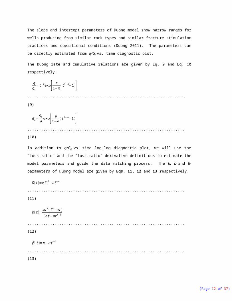
● The Duong model (Duong 2011), and
● The Logistic Growth Model (LGM) (Clark et al. 2011).
Following we will provide a short description of the time–rate models.
Power Law Exponential Model
The power–law exponential model was derived by observing the "loss-ratio" behavior of wells producing
from low/ultra–low permeability reservoirs producing through fracture stimulation. Ilk et al. (2008)
demonstrated that by describing the "loss–ratio" of the data using a power–law function, it is possible to
match the dominant transient and transition flow regimes observed from unconventional reservoirs. In
addition, boundary dominated flow regimes are represented by adding a decline term (D∞) to the power law
relation. The PLE model "loss-ratio" relation is given by Eq. 4.
D( t )=D∞+ Di ntn−1................................................................................................................................(4)
During late-time flow periods, the power-law term becomes less significant and D(t) approaches a constant
term (D∞) similar to the case in Arps exponential decline model. Furthermore, the authors observed that the
derivative of the "loss-ratio" is not constant as was the case in Arps' rate decline relations ( i.e., exponential,
hyperbolic and harmonic equations), but instead it is a function of time. The "loss-ratio" derivative ( b-
β ( t )=D∞+ Di nt n....................................................................................................................................(6)
And the power-law exponential rate relation is given by Eq. 7.
β ( t )=m−at−m......................................................................................................................................(13)
We can also estimate the m parameter independently using the following diagnostic relation:
tGp
qddt [ q
Gp ]=m..................................................................................................................................(14)
Logistic Growth Model
(Page 9 of 28)
Yet another model, the Logistic Growth Model (LGM) is adapted to model time-rate data from oil/gas
reservoirs. The LGM is originally developed to model growth trends of various populations in nature. A
form of the logistic growth model has been used to model growth of yeast and to study market penetration
of new products and technologies (Martinez et al. 2008). Tsoularis and Wallace (2002) have derived a
general form of the logistic growth model. They have also presented a summary of various logistic growth
models for various applications.
Clark (2011) adapted the hyperbolic form of the logistic growth model to match time-rate data of oil/gas
reservoirs. The hyperbolic form was suggested by (Blumberg 1968) to study regenerative growth in nature.
Eq. 15 shows the hyperbolic form of the logistic growth model.
Fluid properties:Gas specific gravity, γg = 0.6 (air = 1)
Hydraulically fractured well model parameters:Fracture half-length, xf = 164.0 ftNumber of fractures = 15Horizontal well length = 4921.3 ft
Production parameters:Flowing pressure, pwf = 500 psiaProduction time, t = 10,958 days (30 years)
Fig. 2 and Fig. 3 shows a "qDb" type diagnostic plot of a time-rated data match using the PLE, LGM and
Duong time-rate relations. The diagnostic relations will provide a systematic and data driven estimation of
the model parameters. When there is no restriction on the degree of freedom, it is possible to obtain a wide
range of parameters that result in a model fit.
(Page 12 of 28)
Figure 2 — (Log-log Plot): qDb type plot ─ flow rate (qg), D- and b- parameter versus production time and time-rate model (PLE, LGM, Duong) matches ─ simulated case (k=800 nD)
(Page 13 of 28)
Figure 3 — (Log-log Plot): qDb type plot ─ flow rate (qg), D- and b- parameter versus production time and time-rate model (PLE, LGM, Duong) matches ─ simulated case (k=50 nD)
.
Fig. 3 shows that the PLE model is capable of modeling all flow regimes including boundary dominated
flow regimes whereas Duong and LGM time-rate relations match transient and transition flow regimes. Fig.
2 and Fig. 3 show that the new time-rate relations are capable of modeling the long transient flow regimes
observed from unconventional reservoirs.
Modified time-rate relations
We have seen that LGM and Duong models fail to match long-time boundary behaviors which leads to
overly optimistic reserve estimate. We have developed new relations based on LGM and Duong time-rate
models of these relations derived by considering long term boundary behaviors. These relations will
provide better time-rate data matches and more reliable EUR estimate. Following is a summary of the
modified new time-rate relations.
(Page 14 of 28)
Modified Duong Model (Model 1)
Rate relation:
qg ( t )=q1 t−mexp [ a1−m
( t1−m−1 )−DDNG t ].......................................................................................(23)
b ( t )=exp[ DLGM t ] tm (exp[ DLGM t ]mtm−at (m+DLGM t ))
(at−exp[ DLGM t ] tm(m+DLGM t ))2 .........................................................................(28)
Modified LGM (Model 3)
Rate relation:
qg ( t )=aKnt (n−1)
(a+ tn )2 exp[−DLGM t ]..........................................................................................................(29)
D-parameter:
D( t )=a (1−n+DLGM t )+tn(1+n+DLGM t )
t (a+tn ) ....................................................................................(30)
b-parameter
b ( t )= −a2(n−1)−2a (n2−1) tn+(n+1) t2 n
(a(1−n+DLGM t )+tn(1+n+DLGM t ))2................................................................................(31)
Modified LGM (Model 4)
Rate relation:
qg ( t )=Ktn−1 a exp[ DLGM t ](n+DLGM t )
(a+(1+R )exp [DLGM t ] tn)2 ...............................................................................................(32)
Cumulative production:
(Page 15 of 28)
Qg( t )=Kt n exp[−DLGM t ]
a+(1+R)exp [ DLGM t ] tn.......................................................................................................(33)
The modified relations are capable of matching long-term time production data obtained from
unconventional reservoirs. These new models constrain the EUR estimates and provide more reliable
production forecasts. Figs. 4 and 5 show the improved match quality of the modified LGM and Duong
time-rate models.
Figure 4 — (Log-log Plot): qDb type plot ─ flow rate (qg), D- and b- parameter versus production time and time-rate model (Duong Model, Modified Duong Model (Model 3), Modified Duong Model (Model 4)) matches ─ simulated case (k=8 µD)
(Page 16 of 28)
Figure 5 — (Log-log Plot): qDb type plot ─ flow rate (qg), D- and b- parameter versus production time and time-rate model (LGM, Modified LGM (Model 3), Modified LGM (Model 4)) matches ─ simulated case (k=8 µD)
We have done model matches of 14 synthetic well models generated using varying permeability values. In
addition, we will investigate the performance of the empirical models in matching production data from
unconventional reservoirs. Also, we will estimate reserves using the “continuous EUR” approach and
compare the performance of the time-rate relations.
6. Development of parametric correlations
Here, we will demonstrate the methodology used to study the relationship between the time-rate model
parameters and the reservoir parameters, specifically permeability (k) and EUR30-Yr. As mentioned earlier,
using the time-rate model diagnostic relations, we can match the time-rate data and estimate the
corresponding model parameters.
(Page 17 of 28)
Figs. 2 and 3 show the diagnostic approach used to model the time-rate data trends. As mentioned earlier,
matching production data is subjective in nature due to the degree of freedom provided by the model
parameters. To obtain consistent and repeatable data matches, we rely on plots of diagnostic relations to
"magnify" trends in the early, middle, and late time periods of the production data. We aim to obtain
quality matches to all flow regimes thereby testing the performance of the rate decline models in matching
the production data. Table 2 summarizes the observed reservoir properties (k and EUR30-Yr) and the
corresponding time-rate model matching parameters when using the PLE model.
Table 2 — Power Law Exponential Model Parameters (14 numerical simulation cases)
Permeability (k),md
qgiMSCF/D
DiD-1
ndimensionless
D∞D-1
EUR30-Yr
BSCF
0.00025 88,607 2.468
0.091 1.8E-05 5.219
0.00050 355,248 3.265
0.078 5.0E-05 7.033
0.00075 896,261 3.834
0.072 7.5E-05 8.113
0.00100 1,792,552 4.273
0.068 9.7E-05 8.829
0.00125 2,503,938 4.419
0.068 1.2E-04 9.343
0.00150 3,249,731 4.529
0.068 1.4E-04 9.739
0.00175 4,608,106 4.742
0.066 1.6E-04 10.018
0.00200 5,937,051 4.875
0.066 1.7E-04 10.240
0.00250 9,396,501 5.139
0.065 2.0E-04 10.585
0.00300 13,723,998
5.362
0.064 2.4E-04 10.799
0.00350 18,706,208
5.543
0.064 2.7E-04 10.967
0.00400 23,653,940
5.666
0.064 3.0E-04 11.082
0.00450 30,171,081
5.816
0.063 3.3E-04 11.170
0.00500 38,246,539
5.973
0.062 3.6E-04 11.245
Next, to provide a basis for developing the parametric correlation, we need to demonstrate how the rate
decline model parameters are related to the reservoir parameters. We will construct a series of cross-plots
to determine how the rate decline model parameters are varying with the reservoir/well properties. Figs. 4 -
6 show permeability plotted against the PLE model parameters and Figs. 7-9 Show EUR30-Yr plotted against
the PLE model parameters. The plots also show results of a regression analysis along with the best fit trend
line function. From the cross-plots it is evident that the PLE model parameters show behaviors that could
(Page 18 of 28)
be described by parametric functions. We will apply similar analysis using Duong and LGM time-rate
relations.
Figure 6 — (Cartesian Plot): Cross plot of permeability and PLE n-Parameter—simulated case.
(Page 19 of 28)
Figure 7 — (Cartesian Plot): Cross plot of permeability and PLE Di -parameter—simulated case.
(Page 20 of 28)
Figure 8 — (Cartesian Plot): Cross plot of permeability and PLE qgi -parameter —simulated case.
Figure 9 — (Cartesian Plot): Cross plot of EUR30-Yr and PLE n-parameter —simulated case.
Figure 10 — (Cartesian Plot): Cross plot of EUR30-Yr and PLE Di -parameter—simulated case.
(Page 21 of 28)
Figure 11 — (Cartesian Plot): Cross plot of EUR30-Yr and PLE-qgi -parameter—simulated case.
The cross-plots describe the relationship between the model parameters and the reservoir properties. The
parametric functions we choose to correlate the individual model parameters with the reservoir properties
should result in a best-fit to the data. The coefficient of determination ("R-squared") value indicates the
accuracy of the selected parametric function in describing the correlation.
The final task is to formulate a function with the rate decline model parameters as variables to estimate the
reservoir properties. Since the rate decline model parameters represent characteristic of the production data
and of the diagnostic relations, it is fair to assume a form of the function that contains the parametric
functions we defined for each model parameter earlier (Figs. 6-11). For example, from Figs. 6-8 we can
see that permeability (k) is related to PLE model parameters, n,Di , and qgi via a power function. From
this we can suggest the following integrating parametric function.
a01 = model parameter, md-D2/MSCFa02 = model parameter, n-parameter exponent, dimensionless
a03 = model parameter Di -parameter exponent, dimensionless
a04 = model parameter qgi -parameter exponent, dimensionless
(Page 22 of 28)
Similarly, EUR can be estimated by the parametric correlation:
EUR=a05 ln ( a06 D i)exp(a07n ) ............................................................................................................(35)
Where:
a05 = model parameter, BSCFa06 = model parameter, Daysa07 = model parameter, dimensionless
Once we establish a form of the parametric equation, we will perform regression analysis to determine the
coefficients and exponents of the parametric correlations. It should be noted that it may not be necessary to
have all time-rate model parameters present in the correlation. Coefficients and exponents that gave best
estimate of the reservoir/well properties are selected. In some cases the exponents or coefficients can
become zero. In such cases, the parameter is eliminated from the final equation. It can be seen that the
qgimodel parameter does not appear in the EUR parametric equation (Eq. 35).
A correlation plot of permeability (k) and EUR30-Yr is shown on Figs. 12 and 1,3 respectively. The figures
show that it is possible to formulate a parametric correlation that estimates reservoir properties from time-
rate relation parameters when reservoir properties such as flowing bottomhole pressure (pwf) and
completion parameters (e.g., number of fracture stages) remain constant. The figures show that the
developed correlations were able to provide a reliable estimate of the reservoir properties.
(Page 23 of 28)
Figure 12 — (Log-log Plot): Comparison of permeability (k) calculated using permeability correlation versus simulated case model permeability.
Figure 13 — (Log-log Plot): Comparison of EUR30-Yr calculated using EUR correlation versus simulated case model EUR30-Yr.
We require that the time-rate relations provide reliable reserve estimates before we attempt to develop the
parametric correlation. Reliable reserve estimate and quality time-rate data match indicates that the model
parameters are related to fundamental reservoir characteristics.
7. Summary and Conclusion
Summary:
In this work we have executed a performance analysis of modern rate decline models (PLE, LGM, and
Duong) using diagnostic relations and diagnostic plots, in matching the production data and estimating
reserves of unconventional reservoirs. We have shown that new time-rate relations are capable of
modeling the dominant transient and transition flow regimes observed from production data analysis of
hydraulically fractured wells in low/ultra-low permeability reservoirs. We have shown that PLE model is
capable of modeling boundary dominated flow regimes whereas LGM and Duong models lack boundary
characteristics. The "continuous EUR" approach is used to study performance of the time-rate models in
estimating ultimate recovery. Finally, we have proposed new time rate-relations to improve the reserve
estimates and production forecasts of these (Duong, LGM) models. The proposed time-rate relations
include boundary conditions to model observed long-time boundary-dominated flow regimes and to
constrain reserve estimates.
(Page 24 of 28)
In addition, we have developed a methodology to formulate a parametric correlation to integrate reservoir
properties with rate decline model parameters by analyzing time-rate data generated from a reservoir
simulation of a multi-fractured horizontal well in low/ultra-low permeability reservoir. The developed
correlations will allow estimation of reservoir properties using parameters of the time-rate models. When
unique estimates of reservoir parameters are missing to allow a complete model based production data
analysis, these correlations will permit fast estimation of fundamental reservoir properties (permeability (k)
and EUR) by using time-rate data which is readily available. This theoretical consideration shows that
when bottomhole flowing pressure is constant, it is possible to correlate empirical time-rate model
parameters with reservoir properties (k and EUR).
Conclusions:
● We have compared performance of PLE, LGM and Duong time-rate relations when used to model
production data from unconventional reservoirs. We have demonstrated various diagnostic relations
and a diagnostic plot method of estimating the model parameters. We have also used the "continuous
EUR" approach to compare degrees of convergence of reserve estimates from these new time-rate
relations.
● We have modified the LGM and Duong time-rate models to obtain relations that can better model
transient, transition and boundary-dominated flow regimes.
● Theoretical consideration for integrating time-rate model parameters with reservoir model parameters
is presented using time-rate data generated from a numerical simulator. The parametric correlations
can provide fast estimates of fundamental reservoir properties when unique estimation is not possible
from model-based production data analysis.
8. Recommendations for Future Work
We have presented a theoretical validation for estimation of reservoir properties using parametric
correlations. Future study will focus on developing the method using a high quality field data.
(Page 25 of 28)
9. Organization of the Research
Following is outline of the proposed research:
● Chapter I — Introduction
■ Statement of problem■ Objectives■ Organization
● Chapter II — Literature Review
■ Empirical, Semi-Analytical, and Empirical Production Data Analysis ■ Integrated Production Data Analysis■ Data Diagnosis■ Reservoir properties from time-rate data analysis
● Chapter III — Analysis of Modern Time-Rate Relations
■ Modern Time-Rate Relations■ Analysis of Time-Rate Data■ Reserve Estimation-"Continuous EUR"■ Modified time-rate relation
● Chapter IV — Development of Parametric Correlation
■ Methodology■ Analysis of Model Parameters■ Parametric Correlation
● Chapter V — Summary and conclusion
■ Summary■ Conclusion■ Recommendation for future work
● Nomenclature
● References
(Page 26 of 28)
Nomenclaturea = Duong model intercept defined by Eq. 7, 1/Db = "Loss-ratio" derivative, dimensionlessa = LGM time-rate equation model parameter (Eq. 13), Daysa01 = Model parameter for empirical correlation, md-D2/MSCFa02 = Model parameter for empirical correlation, dimensionlessa03 = Model parameter for empirical correlation, dimensionlessa04 = Model parameter for empirical correlation, dimensionlessa05 = Model parameter for empirical correlation, BSCFa06 = Model parameter for empirical correlation, Daysa07 = Model parameter for empirical correlation, dimensionless
b = LGM time-rate equation model parameter, DD = "Loss-ratio", 1/DD∞ = Power-law exponential decline relation at infinite time, 1/DDDNG = Modified Duong model decline parameter, 1/D
Di = Power-law exponential decline relation, 1/D DLGM = Modified Duong model decline parameter, 1/DEUR = Estimated ultimate recovery, MSCFEUR30-Yr = Estimated ultimate recovery after 30 years, MSCFk = Model permeability, mdK = LGM model parameter (Carrying capacity), MSCFm = Duong model Slope defined by Eq. 7, dimensionlessn = Power-law exponential relation time exponent, dimensionlessn = LGM time-rate relation model parameter (Eq. 13), dimensionlessq1 = Rate at day 1, MSCF/Dqgi = Power-law exponential relation rate intercept, MSCF/Dt = Production time, daysxf = Fracture half-length, ft
(Page 27 of 28)
References
Arps, J.J. 1945. Analysis of Decline Curves. 945228-G
Clark, A.J. 2011. Decline Curve Analysis in Unconventional Resource Plays Using Logistic Growth Models. M.S Thesis, . The University of Texas at Austin.
Clark, A.J., Lake, L.W., and Patzek, T.W. 2011. Production Forecasting with Logistic Growth Models. Paper presented at the SPE Annual Technical Conference and Exhibition, Denver, Colorado, USA. Society of Petroleum Engineers SPE-144790-MS.
Fetkovich, M.J. 1980. Decline Curve Analysis Using Type Curves. SPE Journal of Petroleum Technology 32 (6). 4629
Fetkovich, M.J., Fetkovich, E.J., and Fetkovich, M.D. 1996. Useful Concepts for Decline Curve Forecasting, Reserve Estimation, and Analysis. SPE Reservoir Engineering 11 (1): 13-22. 28628-PA
Ilk, D., Rushing, J.A., and Blasingame, T.A. 2011. Integration of Production Analysis and Rate-Time Analysis Via Parametric Correlations -- Theoretical Considerations and Practical Applications. Paper presented at the SPE Hydraulic Fracturing Technology Conference, The Woodlands, Texas, USA. 140556.
Ilk, D., Rushing, J.A., Perego, A.D. et al. 2008. Exponential Vs. Hyperbolic Decline in Tight Gas Sands: Understanding the Origin and Implications for Reserve Estimates Using Arps' Decline Curves. Paper presented at the SPE Annual Technical Conference and Exhibition, Denver, Colorado, USA. Society of Petroleum Engineers.
Jay Alan, R., Albert Duane, P., Richard, S. et al. 2007. Estimating Reserves in Tight Gas Sands at Hp/Ht Reservoir Conditions: Use and Misuse of an Arps Decline Curve Methodology. Paper presented at the SPE Annual Technical Conference and Exhibition, Anaheim, California, U.S.A. 109625.
Johnson, R.H. and Bollens, A.L. 1927. The Loss Ratio Method of Extrapolating Oil Well Decline Curves.
Martinez, A.S., González, R.S., and Terçariol, C.A.S. 2008. Continuous Growth Models in Terms of Generalized Logarithm and Exponential Functions. Physica A: Statistical Mechanics and its Applications 387 (23): 5679-5687.
Tsoularis, A. and Wallace, J. 2002. Analysis of Logistic Growth Models. Mathematical Biosciences 179 (1): 21-55. (submitted 2002/8//)
Valko, P.P. 2009. Assigning Value to Stimulation in the Barnett Shale: A Simultaneous Analysis of 7000 Plus Production Histories and Well Completion Records. Paper presented at the SPE Hydraulic Fracturing Technology Conference, The Woodlands, Texas. Society of Petroleum Engineers SPE-119369-MS.