Meta-Unsupervised-Learning: A supervised approach to unsupervised learning Vikas K. Garg and Adam Tauman Kalai December 29, 2016 Abstract We introduce a new paradigm to investigate unsupervised learning, reducing unsupervised learning to supervised learning. Specifically, we mitigate the subjectivity in unsupervised decision-making by leveraging knowledge acquired from prior, possibly heterogeneous, supervised learn- ing tasks. We demonstrate the versatility of our framework via com- prehensive expositions and detailed experiments on several unsupervised problems such as (a) clustering, (b) outlier detection, and (c) similar- ity prediction under a common umbrella of meta-unsupervised-learning. We also provide rigorous PAC-agnostic bounds to establish the theoret- ical foundations of our framework, and show that our framing of meta- clustering circumvents Kleinberg’s impossibility theorem for clustering. 1 Introduction Unsupervised Learning (UL) is an elusive branch of machine learning, includ- ing problems such as clustering and manifold learning, that seeks to identify structure among unlabeled data. Unsupervised learning is notoriously difficult to evaluate, and debates rage about which objective function to use, since the absence of data labels makes it difficult to define objective quality measures. This paper proposes a meta-solution that, by considering the (meta)distribution over unsupervised problems, reduces UL to Supervised Learning (SL). This is a data-driven approach to quantitatively evaluate and design new UL algorithms. Going beyond typical transfer learning, we show how this approach can be used for to improve UL performance for problems of different sizes and from different domains. As a thought-provoking example, consider clustering the course reviews in Figure 1. The clustering based on sentiment, done by a human, is clearly more “human” than the one based on word count, done by machine. How do humans learn to cluster in this way, and how can computers learn to cluster in this way? People would identify the text as English and may recall related text challenges they have faced, as opposed to image tasks. They may also draw on knowledge about courses. We argue that computers should identify and leverage data from related prior tasks, such as text corpora, clustered documents, clustered reviews, or even clustered course reviews if available. A die-hard K-means advocate may say that the K-means objective of average distance to cluster centers is right, and that the bag-of-words representation used for computing distances is 1 arXiv:1612.09030v1 [cs.LG] 29 Dec 2016
Transcript
Meta-Unsupervised-Learning:
A supervised approach to unsupervised learning
Vikas K. Garg and Adam Tauman Kalai
December 29, 2016
Abstract
We introduce a new paradigm to investigate unsupervised learning,reducing unsupervised learning to supervised learning. Specifically, wemitigate the subjectivity in unsupervised decision-making by leveragingknowledge acquired from prior, possibly heterogeneous, supervised learn-ing tasks. We demonstrate the versatility of our framework via com-prehensive expositions and detailed experiments on several unsupervisedproblems such as (a) clustering, (b) outlier detection, and (c) similar-ity prediction under a common umbrella of meta-unsupervised-learning.We also provide rigorous PAC-agnostic bounds to establish the theoret-ical foundations of our framework, and show that our framing of meta-clustering circumvents Kleinberg’s impossibility theorem for clustering.
1 Introduction
Unsupervised Learning (UL) is an elusive branch of machine learning, includ-ing problems such as clustering and manifold learning, that seeks to identifystructure among unlabeled data. Unsupervised learning is notoriously difficultto evaluate, and debates rage about which objective function to use, since theabsence of data labels makes it difficult to define objective quality measures.This paper proposes a meta-solution that, by considering the (meta)distributionover unsupervised problems, reduces UL to Supervised Learning (SL). This is adata-driven approach to quantitatively evaluate and design new UL algorithms.Going beyond typical transfer learning, we show how this approach can be usedfor to improve UL performance for problems of different sizes and from differentdomains.
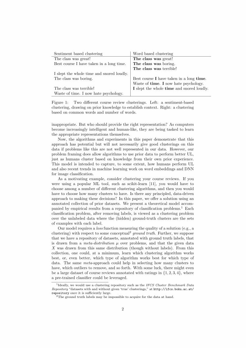
As a thought-provoking example, consider clustering the course reviews inFigure 1. The clustering based on sentiment, done by a human, is clearly more“human” than the one based on word count, done by machine. How do humanslearn to cluster in this way, and how can computers learn to cluster in this way?People would identify the text as English and may recall related text challengesthey have faced, as opposed to image tasks. They may also draw on knowledgeabout courses. We argue that computers should identify and leverage data fromrelated prior tasks, such as text corpora, clustered documents, clustered reviews,or even clustered course reviews if available. A die-hard K-means advocatemay say that the K-means objective of average distance to cluster centers isright, and that the bag-of-words representation used for computing distances is
1
arX
iv:1
612.
0903
0v1
[cs
.LG
] 2
9 D
ec 2
016
Sentiment based clustering Word based clusteringThe class was great! The class was great!Best course I have taken in a long time. The class was boring.
The class was terrible!I slept the whole time and snored loudly.The class was boring. Best course I have taken in a long time.
Waste of time. I now hate psychology.The class was terrible! I slept the whole time and snored loudly.Waste of time. I now hate psychology.
Figure 1: Two different course review clusterings. Left: a sentiment-basedclustering, drawing on prior knowledge to establish context. Right: a clusteringbased on common words and number of words.
inappropriate. But who should provide the right representation? As computersbecome increasingly intelligent and human-like, they are being tasked to learnthe appropriate representations themselves.
Now, the algorithms and experiments in this paper demonstrate that thisapproach has potential but will not necessarily give good clusterings on thisdata if problems like this are not well represented in our data. However, ourproblem framing does allow algorithms to use prior data to perform better UL,just as humans cluster based on knowledge from their own prior experience.This model is intended to capture, to some extent, how humans perform ULand also recent trends in machine learning work on word embeddings and DNNfor image classification.
As a motivating example, consider clustering your course reviews. If youwere using a popular ML tool, such as scikit-learn [11], you would have tochoose among a number of different clustering algorithms, and then you wouldhave to choose how many clusters to have. Is there any principled, data-drivenapproach to making these decisions? In this paper, we offer a solution using anannotated collection of prior datasets. We present a theoretical model accom-panied by empirical results from a repository of classification problems.1 Eachclassification problem, after removing labels, is viewed as a clustering problemover the unlabeled data where the (hidden) ground-truth clusters are the setsof examples with each label.
Our model requires a loss function measuring the quality of a solution (e.g., aclustering) with respect to some conceptual2 ground truth. Further, we supposethat we have a repository of datasets, annotated with ground truth labels, thatis drawn from a meta-distribution µ over problems, and that the given dataX was drawn from this same distribution (though without labels). From thiscollection, one could, at a minimum, learn which clustering algorithm worksbest, or, even better, which type of algorithm works best for which type ofdata. The same meta-approach could help in selecting how many clusters tohave, which outliers to remove, and so forth. With some luck, there might evenbe a large dataset of course reviews annotated with ratings in {1, 2, 3, 4}, wherea pre-trained classifier could be leveraged.
1Ideally, we would use a clustering repository such as the IFCS Cluster Benchmark DataRepository “datasets with and without given ‘true’ clusterings,” at http://ifcs.boku.ac.at/repository once it is sufficiently large.
2The ground truth labels may be impossible to acquire for the data at hand.
2
Our theoretical model, closely related to Agnostic [8] and PAC Learning[19], treats each entire labeled problem analogous to an training example in asupervised learning task. We show how one can provably learn to perform ULas well as the best algorithm in certain classes of algorithms.
Empirically, we run meta-algorithms on the repository of classification prob-lems from openml.org which has a variety of datasets from various domainsincluding NLP, computer vision, and bioinformatics, among others. Ignoringlabels, each dataset can be viewed as an unsupervised learning problem. In-terestingly, we find that this seemingly unrelated collection of problems can beleveraged to improve average performance across datasets. In particular, wefirst find that the K-means clustering algorithm generally outperforms four oth-ers across the collection of problems. While this is not surprising in the sensethat K-means is one of the most popular clustering algorithms, our finding isbased upon data and not simply “word of mouth.” Second, we show that thereare systematic but correctable biases among a standard heuristic for selectingthe number of clusters. Third, we show how the data can be used to decidehow many outliers to remove to improve clustering performance. Finally, wealso show how to train a neural network using data from multiple classifica-tion problems of very different natures to improve performance on a new ULproblem.
In some sense, this meta-approach is arguably being used by today’s NLPand computer vision practitioners, as well as by humans. For instance, whena human clusters course reviews, they heavily use their knowledge of Englishthat has been already acquired from a number of other learning tasks. Sim-ilarly, modern NLP algorithms rely upon Word Embeddings [14] that encodethe meanings of words in a constant number of dimensions and are trained onother text corpora or billions of words. In some sense, expecting an algorithm tocluster a small set of text reviews without external data is like asking a personto cluster course reviews written in a foreign language without a dictionary –not only would one have to learn the new language from the reviews themselvesbut there might not even be enough reviews to adequately cover the language.Similarly, a recent theme in computer vision, given a set of thousands of im-ages, is to re-use pieces of neural networks trained on a labeled set of millionsof images.
2 Related work
This work relates to and unifies a number of areas within machine learning. Inunsupervised learning, the frustrating sense of futility in debating the “best”clustering algorithm is conveyed by Kleinberg’s impossibility theorem for clus-tering [9], though his axioms have been the subject of further debate [20, 1]. InSection 5, we show how meta-clustering circumvents this impossibility in somesense.
Some supervised approaches [4], [6] have been proposed to learn a clusteringfunction, using a dataset where each instance is comprised a set of homogeneousitems (such as news articles) and their partitioning into clusters. The learnedfunction could then be used to cluster a new set of items of the same kind.Our approach generalizes the notion by learning across heterogeneous datasetsthat are compiled from several domains, to find a good clustering for new data.
3
These domains may have data represented with different dimensionalities.Our framework can also be viewed as taking an extreme viewpoint of transfer
learning. The body of work on (supervised) transfer learning is too large tosurvey here, see e.g., [10] and references therein. Our work can be viewed asmore extreme than typical transfer learning in that the multiple source datasetsmight have completely different distributions and data generating processes fromeach other, and from the (multiple) test datasets. As mentioned, typically intransfer learning the problems have the same dimensionality or at least the sametype of data (text, images, etc.), whereas our experiments consist of varied datatypes. Unlike many transfer learning methods, we do not use the features fromtest data during training.
Our work also relates to supervised learning questions of meta-learning,sometimes referred to as auto-ml (e.g., [16, 5]), learning to learn (e.g., [18]),Bayesian optimization (e.g., [15]) and lifelong learning (e.g., [17, 3]). In thecase of supervised learning, where accuracy is easy to evaluate, meta-learningenables algorithms to achieve accuracy more quickly with less data. We arguethat for unsupervised learning, the meta approach offers a principled means ofdefining and evaluating unsupervised learning.
3 Learning Preliminaries
A learning task consists of a universe X , labels Y, outputs Z, and a bounded lossfunction ` : X × Y ×Z → [0, 1]. A learner L : (X × Y)∗ → ZX takes a trainingset T = (X1, Y1), . . . (Xn, Yn) consisting of a finite number of iid samples fromµ and outputs a classifier L(T ) ∈ ZX , which denotes the set of functions fromX to Z. The loss of a classifier c ∈ ZX is `µ(c) = E(X,Y )∼µ [`(X,Y, c(X))], andthe expected loss of L is `µ(L) = ET∼µn [`µ(L(T ))].
Meta-unsupervised-learning is a special case of supervised learning. Thereare two subtle differences. The first is conceptual: the output of a meta-unsupervised-learning algorithm is an unsupervised algorithm (e.g., a clusteringalgorithm) and the training examples are entire data sets. Also note that, whilewe require the training data to be fully labeled (e.g., clustered/classified), wemay never see the true clusters of any problem encountered after deployment.This is different than online learning, where it is assumed that for each exam-ple, after you make a prediction, you find out the ground truth. The seconddifference is that Z 6= Y, the output of the algorithm may or may not be ofthe same “type” as the ground truth labels. For instance, in feature selectionthe output may be a subset of the features whereas the training data may haveclassification labels, and the loss function connects the two.
Learning is with respect to a concept class C ⊆ ZX .
Definition 1 (Agnostic learning of C). For countable sets3 X ,Y,Z and ` :X × Y × Z → [0, 1], a learner L agnostically learns A ⊆ ZX if there existsa polynomial p such that for any distribution µ over X × Y and for any n ≥p(1/ε, 1/δ),
PrT∼µn
[`µ(L(T )) ≤ min
c∈C`µ(c) + ε
]≥ 1− δ.
3For simplicity of presentation, we assume that these sets are countable, but with appro-priate measure theoretic assumptions the analysis in this paper extends to infinite cases in astraightforward manner.
4
Further, L and the classifier L(T ) must run in time polynomial in the length oftheir inputs.
PAC learning refers to the special case where an additional assumption isplaced on µ such that minc∈C `µ(c) = 0. A learner L is called proper if it onlyoutputs classifiers in C. We call the task homogeneous if Y = Z. (Most taskswe consider will be homogeneous.)
3.1 Meta-unsupervised-learning definitions
Meta-unsupervised-learning, which is henceforth the focus of this paper, simplyrefers to case where µ is a meta-distribution over datasets X ∈ X and groundtruth labelings Y ∈ Y, and classifiers c are unsupervised learning algorithmsthat take an entire dataset X as input, such as clustering algorithms. Unlikeonline learning, as mentioned, true labels are only observed for the trainingdatasets.
3.1.1 Meta-clustering
For a finite set S, the clusterings Π(S) denotes the set of disjoint partitions of Sinto 2 or more sets, e.g., Π({1, 2, 3}) =
{{{1}, {2, 3}}, {{2}, {1, 3}}, {{1, 2}, {3}}
}.
For a clustering C, denote by ∪C = ∪S∈CS the set of points clustered. We as-sume that each X ∈ X is a finite set of two or more elements and
Y = Z ={
Π(X) | X ∈ X}.
The loss function defined below is 1 if the clusterings are invalid.4 To define theloss, for clustering C, we first define the distance function dC(x, x′) to be 0 ifthey are in the same cluster, i.e., x, x′ ∈ S for some S ∈ C, i.e., and 1 otherwise.The loss will be the following clustering distance,
`(X,Y, Z) =
1
|X|(|X| − 1)
∑
x,x′∈X|dY (x, x′)− dZ(x, x′)| if Y, Z ∈ Π(X)
1 otherwise
(1)
where |S| denotes the size of set S. In words, this is the fraction of pairs ofdistinct points where the two clusterings differ on whether or not the two pointsare in the same cluster. Note that this loss is 1 − RI(Y, Z), where RI is theso-called Rand Index, one of the most common measures of clustering accuracywith respect to a ground truth. In our experiments, the loss we will measure isthe standard Adjusted Rand Index (ARI) which attempts to correct the RandIndex by accounting for chance agreement [7]. We denote by ARI(Y,Z) theadjusted rand index between two clusterings Y and Z. We abuse notation andalso write ARI(Y, Z) when Y is a vector of class labels, by converting it to aper-class clustering with one cluster for each class label.
We refer to the problem of clustering into k=2 clusters as 2-clustering.In Euclidean clustering, the points are Euclidean, so each dataset X ⊂ Rd
for some d ≥ 1. Note that different datasets may have different dimensionalities
4It would be natural to impose the requirement that ∪Y = X with probability 1 over µ,but this is not formally necessary as all clustering algorithms c ∈ C have ∪c(X) = X andhence incur loss of 1 in the case that ∪Y 6= X.
5
d. Other frameworks could be modeled, e.g., in list clustering (see, e.g., [2])where the algorithm outputs a bounded list of clusterings Z = (Z1, . . . , Zl), theloss could be mini d(Y,Zi).
Rand Index measures clustering quality with respect to an extrinsic groundtruth. In many cases, such a ground truth is unavailable, and an intrinsic metricis useful. Such is the case when choosing the number of clusters. Given differentclusterings of size k = 2, 3, . . ., how can one compare and select? One approachis the so-called silhouette score [12], defined as follows for a Euclidean clustering:
sil(C) =1
| ∪ C|∑
x∈∪C
b(x)− a(x)
max{a(x), b(x)} , (2)
where a(x) denotes the average distance between point x and other points inits own cluster and b(x) denotes the average distance between x and points inan alternative cluster, where the alternative cluster is the one whose minimumaverage distance to x is smallest among those clusters different than the onecontaining x.
4 Meta-unsupervised-ERM
The simplest approach to meta-unsupervised-learning is Empirical Risk Mini-mization (ERM), namely choosing the unsupervised algorithm from some familyC with lowest empirical error on training set T , which we write as ERMC(T ).Standard learning bounds imply a logarithmic dependence on the size of thefamily.
Lemma 1. For any finite family C of unsupervised learning algorithms, anydistribution µ over problems X,Y ∈ X × Y, and any m ≥ 1, δ > 0,
PrT∼µn
[`µ(ERMC(T )) ≤ min
c∈C`µ(c) +
√2
nlog|C|δ
]≥ 1− δ,
where ERMC(T ) ∈ arg minc∈C∑T `(Y, c(X)) is any empirical loss minimizer
over c ∈ C.
This standard generalization bound, which follows from Chernoff and unionbounds, suffices to bound the performance of ERM over finite sets of unsuper-vised learning algorithms.
Selecting among algorithms. An immediate corollary is that, given m clus-tering algorithms, one can perform within O(
√log(m)/n) as the best by evalu-
ating all clustering algorithms on a training set of n clustering problems (withground truths) and choosing the best.
Fitting a parameter. Next, consider choosing the threshold parameter of asingle linkage clustering algorithm. Fix the set of possible vertices V. Take theuniverse X to consist of undirected weighted graphs X = (V,E,W ) with verticesV ⊆ V, edges E ⊆ {{u, v} | u, v ∈ V } and non-negative weights W : E → R+.Data in Rd can be viewed as a complete graph in with W ({x, x′}) = ‖x− x′‖.
The prediction and output sets are simply Y = Z = Π(V) the sets of parti-tions of vertices, and the loss is defined as in Eq. (1). The classic single-linkageclustering algorithm with parameter r ≥ 0, Lr(V,E,w), creates as clusters the
6
connected components of the subgraph of (V,E) consisting of all edges whoseweights are less than or equal to r. That is, u, v ∈ V are in the same cluster ifand only if there is a path from u to v where all edges in the path have weightsat most r.
It is trivial to see that one can find the best cutoff for r in polynomial time:for each edge weight r in the set of edge weights across all graphs, computethe mean loss of Lr across the training set. Since Lr runs in polynomial time,loss can be computed in polynomial time, and the number of different possiblecutoffs is bounded by the number of edge weights which is polynomial in theinput size, the entire algorithm runs in polynomial time.
For a quasilinear-time algorithm (in the input size |T | = Θ(∑i |Vi|2)), run
Kruskal’s algorithm on the union graph of all of the graphs in the training set(i.e., the number of nodes and edges are the sum of the number of nodes andedges in the training graphs, respectively). As Kruskal’s algorithm adds eachnew edge to its forest (in order of non-decreasing edge weight), effectively twoclusters in some training graph (Vi, Ei,Wi) have been merged. The change inloss of the resulting clustering can be computed from the loss of the previousclustering in time proportional to the product of the two clusters that are beingmerged, since these are the only values on which Zi changed. Naively, thismay seem to take order
∑i |Vi|3. However, note that, each pair of nodes begins
separately and is updated, exactly once during the course of the algorithm, to bein the same cluster. Hence, the total number of updates is O(
∑i |Vi|2), and since
Kruskal’s algorithm is quasilinear time itself, the entire algorithm is quasilinear.For correctness, it is easy to see that as Kruskal’s algorithm runs, Lr has beencomputed for each possible r at the step just preceding when Kruskal adds thefirst edge whose weight is greater than r.
For generalization bounds, let us simply assume that numbers are repre-sented with some constant b number of bits, as is common on all modern com-puters. By Lemma 1, we see that with m training graphs and |{Lr}| ≤ 2b, wehave that with probability ≥ 1−δ, the error of ERM is within
√2(b+ log 1/δ)/n
of minr `µ(Lr). Combining this argument with the efficient algorithm, proves:
Theorem 1. The class {Lr | r > 0} of single-linkage algorithms with thresholdr (where numbers are represented using b bits), can be agnostically learned.In particular, a quasilinear time algorithm achieves error ≤ minr `µ(Lr) +√
2(b+ log 1/δ)/n, with probability ≥ 1− δ over the n training problems.
4.1 Meta-K: choosing the number of clusters, k
We now discuss a meta approach to choosing the number of clusters, a cen-tral problem in clustering. we refer to this as the Meta-K problem: selectingamong the output of a base clustering algorithm that outputs one clusteringwith k clusters for each k ∈ {2, 3, . . . ,K} in a bounded range. Clearly, we re-quire additional information as different clustering problems require differentnumbers of clusters. This additional “meta-information” includes informationspecific to the clustering and to the problem. In particular, suppose that eachproblem X encodes, among other things, a set of points V to be clustered andproblem metadata φ ∈ Φ. Also, suppose that the base algorithm producesclusterings (C2, γ2), . . . , (CK , γK) ∈ CV × Γ where Ck has k clusters and γkis meta-information about the clustering. For instance, one common type of
7
meta-information would be some clustering quality heuristic such as the silhou-ette score for a clustering as defined in eq. (2). However, instead of simplychoosing the clustering maximizing silhouette score, we can learn how to choosethe best clustering based on k, φ, and γk.
Given a family F of functions f : Φ × ΓK−1 → {2, . . . ,K} that select thenumber of clusters, as long as F can be parametrized by a fixed number ofb-bit numbers, the ERM approach of choosing the “best” f will be statisticallyefficient. If, for training problem Xi, the metadata is φi and clustering algorithmoutputs (Ci2, γi2), . . . , (CiK , γiK), then ERM amounts to:
ERMF = arg minf∈F
∑
i
`(Xi, Yi, Cif(φi,γi2,...,γiK)
).
The final clustering algorithm output would be ERMf run among the outputof the base clustering algorithm. If ERMf cannot be computed exactly withintime constraints, an approximate minimizer may be used.
4.2 Meta-outlier-removal
For simplicity, we consider learning the single hyperparameter of the fraction ofexamples, furthest from the mean, to remove. In particular, suppose trainingproblems are classification instances, i.e., Xi ∈ Rdi×mi and Yi ∈ {1, 2, . . . , ki}mi .This problem could apply to clustering or any other unsupervised learning al-gorithm. For this section, we assume that the base classifier algorithm (e.g.,clustering algorithm) takes a parameter θ which is how many outliers to ignoreduring fitting.
For instance, in clustering, given an algorithm C, one might define Cθ withparameter θ ∈ [0, 1) on data x1, . . . , xn ∈ Rd as follows:
1. Compute the data mean µ = 1n
∑i xi.
2. Set aside as outliers the θ examples where xi is furthest from µ in Euclideandistance.
3. Run the base clustering algorithm C on the data with outliers removed.
4. Assign each outlier to the cluster whose center it is closest to.
We can then compute the loss of the resulting output Z and the groundtruth Y , for any dataset. Given a meta-dataset of n datasets, we choose θ soas to optimize performance. With a single b-bit parameter θ, Lemma 1 easilyimplies that this choice of θ will give a loss within
√2(b+ log 1/δ)/n of the
optimal θ, with probability ≥ 1 − δ of the sample of datasets. The number ofθ’s that need to be considered is bounded by the total number of inputs acrossproblems, so the meta-algorithm runs in polynomial time.
4.3 Problem recycling
For this model, suppose that each problem belongs to a set of common problemcategories, e.g., digit recognition, sentiment analysis, image classification amongthe thousands of classes of ImageNet [13], etc. The idea is that one can recyclethe solution to one version of the problem in a later incarnation. For instance,
8
suppose that one trained a digit recognizer on a previous problem. For a newproblem, the input may be encoded differently (e.g., different image size, differ-ent pixel ordering, different color representation), but there is a transformationT that maps this problem into the same latent space as the previous problemso that the prior solution can be re-used.
In particular, for each problem category i = 1, 2, . . . , N , there is a latentproblem space Λi and a solver Si : Λi → Zi. Each problem X,Y of this categorycan be transformed to T (X) ∈ Λi with low solution loss `(X,Y, S(T (X))). Notethat one of these categories could be “miscellaneous,” a catch-all category whosesolution could be another unsupervised (or meta-unsupervised) algorithm.
A problem recycling model consists of three components:
• Solvers Si : Λi → Zi, for i = 1, 2, . . . , N , where each solver operates overa latent space Λi.
• A (meta)classifier M : X → {1, 2, . . . , N} that, for a problem X, identifieswhich solver i = M(X) to use.
• Transformation procedures Ti : M−1(i)→ Li that maps any X such thatM(X) = i into latent space Λi.
The output of the meta-classifier is simply SM(X)(TM(X)(X)). Lemma 1 impliesthat if one can optimize over meta-classifiers and the parameters of the meta-classifier are represented by D b-bit numbers, then one achieves loss within ε ofthe best meta-classifier with m = O
(Db/ε2
)problems.
5 The possibility of meta-clustering
In this section, we point out how the framing of meta-clustering circumventsKleinberg’s impossibility theorem for clustering [9]. To review, Kleinberg con-siders clustering finite sets of points X endowed with symmetric distance func-tions d ∈ D(X), where the set of valid distance functions is:
D(X) = {d : X×X → R | ∀x, x′ ∈ X d(x, x′) = d(x′, x) ≥ 0, d(x, x′) = 0 iff x = x′}.
A clustering algorithm A takes a distance function d ∈ D(X) and returns apartition, i.e., A(d) ∈ Π(X).
He defines the following three axioms that should hold for any clusteringalgorithm A:
1. Scale-Invariance. For any distance function d and any α > 0, A(d) =A(α · d), where α · d is the distance function d scaled by α.
2. Richness. For any finite X and clustering C ∈ Π(X), there exists adistance d ∈ D(X) such that A(d) = C.
3. Consistency. Let d, d′ ∈ D(X) such that A(d) = C, and for all x, x′ ∈ X,if x, x′ are in the same cluster in C then d′(x, x′) ≤ d(x, x′) while if x, x′
are in different clusters in C then d′(x, x′) ≥ d(x, x′). Then A(d′) = A(d).
The key difficulty to defining clustering is to establish a scale. To get intuitionfor why, consider clustering two points X = {x1, x2} so there is a single distance
9
in the problem. For a moment, consider allowing the trivial clustering into asingle cluster, so there are two legal clusterings {{x1, x2}} and {{x1}, {x2}}. Tosee that axioms 1 and 2 are impossible to satisfy note that, by richness, theremust be some distances δ1, δ2 > 0 such that if d(x1, x2) = δ1 then they are in thesame cluster while if d(x1, x2) = δ2 they are in different clusters. This, howeverviolates Scale-Invariance, since the two problems are at a scale α = δ2/δ1 of eachother. Now, this example fails to hold when there are two or more clusters, butit captures the essential intuition.
Now, suppose we define the clustering problem with respect to a non-emptytraining set of clustering problems. So a meta-clustering algorithm takes t ≥ 1training clustering problems M(d1, C1, . . . , dt, Ct) = A with their ground-truthclusterings (on corresponding sets Xi, i.e., di ∈ D(Xi) and Ci ∈ Π(Xi)) andoutputs a clustering algorithm A. We can use these training clusterings toestablish a scale.
In particular, we will show a meta-clustering algorithm whose output Aalways satisfies the second two axioms and which satisfies the following variantof Scale-Invariance:
1. Meta-Scale-Invariance. Fix any distance functions d1, d2, . . . , dt andground truth clusterings C1, . . . , Ct on sets X1, . . . , Xt. For any α > 0,and any distance function d, if M(d1, C1, . . . , dt, Ct) = A and M(α ·d1, C1, . . . , α · dt, Ct) = A′, then A(d) = A′(α · d).
With meta-clustering, the scale can be established using training data.
Theorem 2. There is a meta-clustering algorithm that satisfies Meta-Scale-Invariance and whose output always satisfies Richness and Consistency.
Proof. There are a number of such clustering algorithms, but for simplicity wecreate one based on single-linkage clustering. Single-linkage clustering satisfiesRichness and Consistency (see [9], Theorem 2.2). The question is how to chooseit’s single-linkage parameter. One can choose it to be the minimum distancebetween any two points in different clusters across all training problems. It iseasy to see that if one scales the training problems and d by the same factorα, the clusterings remain unchanged, and hence the meta-clustering algorithmsatisfies meta-scale-invariance.
6 Experiments
We conducted several experiments to substantiate the efficacy of the proposedframework under various unsupervised settings. We downloaded all classifica-tion datasets from OpenML5 that had at most 10,000 instances, 500 features,10 classes, and no missing data to obtain a corpus of 339 datasets. For our pur-poses, we extracted the numeric features from all these datasets ignoring thecategorical features. We now describe in detail the results of our experiments,highlighting the gains achieved due to our meta paradigm.
5http://www.openml.org .
10
6.1 Selecting an algorithm
As a first step, we consider the question of which of a number of given clusteringalgorithms to use to cluster a given data set. In this section, we focus on k = 2clusters. Later, we consider meta-algorithms for choosing the number of clusters.
First, one can run each of the algorithms on the repository and see whichalgorithm has the lowest average error. Error is calculated with respect to theground truth labels by the ARI (see Section 3). We compare algorithms onthe 250 openml binary classification datasets with at most 2000 instances. Theten base clustering algorithms were chosen to be five clustering algorithms fromscikit-learn (K-Means, Spectral, Agglomerative Single Linkage, Complete Link-age, and Ward) together with a second version of each in which each attributeis first normalized to have zero mean and unit variance. Each algorithm is runwith the default scikit-learn parameters.
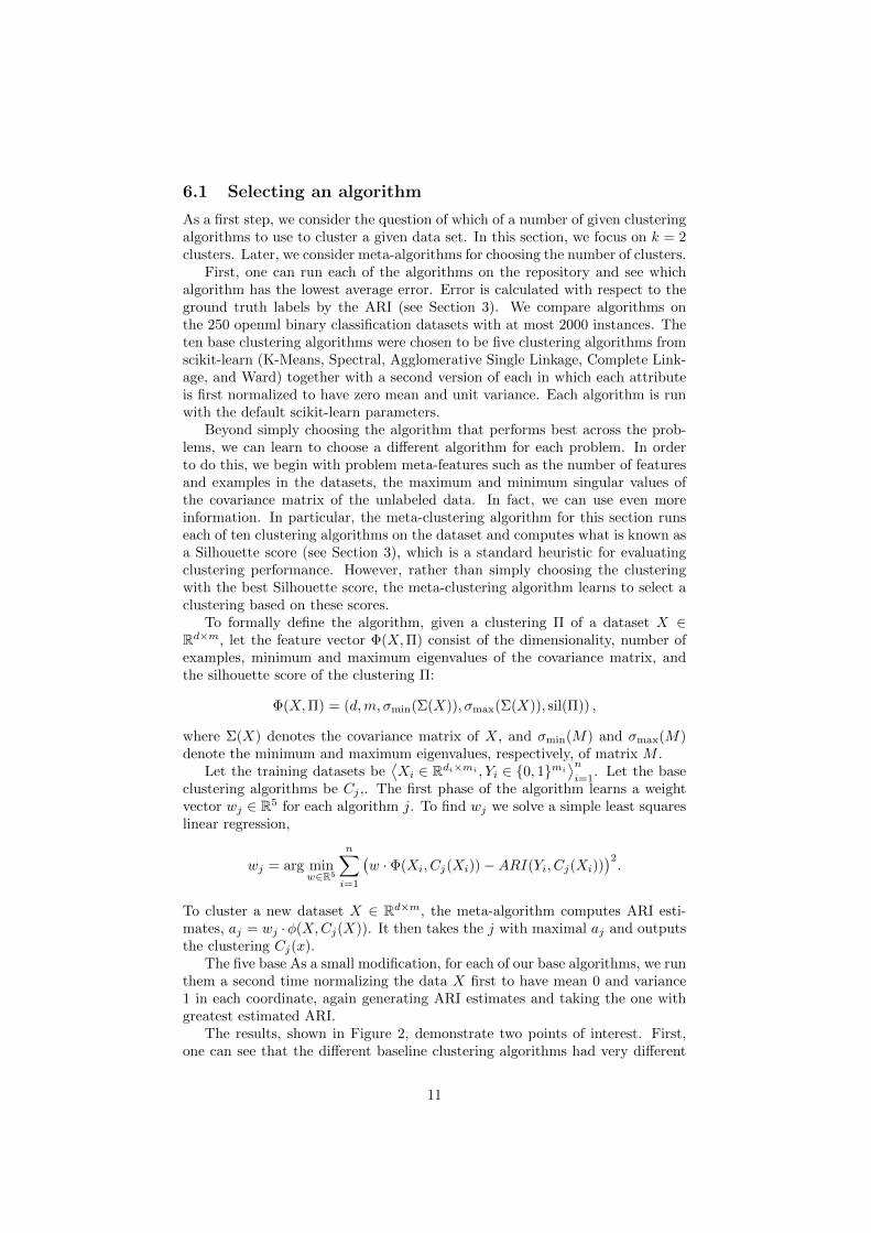
Beyond simply choosing the algorithm that performs best across the prob-lems, we can learn to choose a different algorithm for each problem. In orderto do this, we begin with problem meta-features such as the number of featuresand examples in the datasets, the maximum and minimum singular values ofthe covariance matrix of the unlabeled data. In fact, we can use even moreinformation. In particular, the meta-clustering algorithm for this section runseach of ten clustering algorithms on the dataset and computes what is known asa Silhouette score (see Section 3), which is a standard heuristic for evaluatingclustering performance. However, rather than simply choosing the clusteringwith the best Silhouette score, the meta-clustering algorithm learns to select aclustering based on these scores.
To formally define the algorithm, given a clustering Π of a dataset X ∈Rd×m, let the feature vector Φ(X,Π) consist of the dimensionality, number ofexamples, minimum and maximum eigenvalues of the covariance matrix, andthe silhouette score of the clustering Π:
Φ(X,Π) = (d,m, σmin(Σ(X)), σmax(Σ(X)), sil(Π)) ,
where Σ(X) denotes the covariance matrix of X, and σmin(M) and σmax(M)denote the minimum and maximum eigenvalues, respectively, of matrix M .
Let the training datasets be⟨Xi ∈ Rdi×mi , Yi ∈ {0, 1}mi
⟩ni=1
. Let the baseclustering algorithms be Cj ,. The first phase of the algorithm learns a weightvector wj ∈ R5 for each algorithm j. To find wj we solve a simple least squareslinear regression,
wj = arg minw∈R5
n∑
i=1
(w · Φ(Xi, Cj(Xi))−ARI(Yi, Cj(Xi))
)2.
To cluster a new dataset X ∈ Rd×m, the meta-algorithm computes ARI esti-mates, aj = wj ·φ(X,Cj(X)). It then takes the j with maximal aj and outputsthe clustering Cj(x).
The five base As a small modification, for each of our base algorithms, we runthem a second time normalizing the data X first to have mean 0 and variance1 in each coordinate, again generating ARI estimates and taking the one withgreatest estimated ARI.
The results, shown in Figure 2, demonstrate two points of interest. First,one can see that the different baseline clustering algorithms had very different
Figure 2: Adjusted Rand Index (ARI) scores of different clustering (k=2) al-gorithms on 250 openml binary classification problems. The meta algorithm iscompared with standard clustering baselines on both the original data as wellas the transformed data where all features in the datasets were normalized tohave zero mean and unit variance (denoted by the suffix “-N”). The figure shows95% confidence intervals for the meta approach.
average performances. Hence, a practitioner with unlabeled data (and hence lit-tle means to evaluate the different algorithms), may very likely choose a randomalgorithm and suffer poor performance. If one had to choose a single algorithm,K-means with normalization performed best. Perhaps this is not surprising asK-means is arguably the most popular clustering algorithm, and normalizationis a common preprocessing step. However, our experiment justifies this choicebased on evaluation across problems from the openml repository.
Second, Figure 2 also demonstrates that the meta-algorithm, given suffi-ciently many training problems, is able to outperform, on average, all the base-line algorithms. This is despite the fact that the 250 problems have differentdimensionalities and come from different domains.
6.2 Meta-K
For the purposes of this section, we fix the clustering algorithm to be K-meansand compare two approaches to choosing the number of clusters, k from k = 2to 10. First, we consider a standard heuristic for the baseline choice of k: foreach cluster size k and each dataset, we generate 10 clusterings from differentrandom starts for K-means and take one with best Silhouette score among the
12
10. Then, over the 9 different values of k, we choose the one with greatestSilhouette score so that the resulting clustering is the one of greatest Silhouettescore among all 90.
Similar to the approach for choosing the best algorithm above, in our meta-Kapproach, we learn to choose k as a function of Silhouette score and k by choosingthe k with highest estimated ARI. As above, for any given problem and anygiven k, among the 10 clusterings, we choose the one that maximizes Silhouettescore. However, rather than simply choosing k that maximizes Silhouette score,we choose k to maximize a linear estimate of ARI that varies based on both theSilhouette score and k. We evaluate on exactly the same 90 clusterings for ofthe 339 datasets as the baseline.
We computed the Silhouette scores and Adjusted Rand Index (ARI) scoresfor each of the 339 datasets from k = 2 to 10. We conducted 10 such independentexperiments for each dataset to account for statistical significance, and thusobtained two 90-dimensional vectors per dataset for Silhouette and ARI scores.Moreover, as is standard in the clustering literature, we assumed the best-fit k∗ifor dataset i to be the one that yielded maximum ARI score across the differentruns, which is often different from ki, the number of clusters in the ground truth,i.e., the number of class labels.
The training and test sets were obtained using the following procedure. Eachof the 339 datasets were designated to be either a training set or test set. Thenumber of training sets was varied over a wide range to take values in the set{140, 160, . . . , 280}. For each such split size, the training examples from thedifferent sets together formed the meta-training set, and the remaining setsformed the meta-test set. Thus, 8 such (training, test) partitions were obtainedcorresponding to these sizes.
For any particular partition into training and test sets, we followed a regres-sion procedure to estimate the ARI score as a function of the Silhouette score.Specifically, for each k ∈ {2, . . . , 9}, we fit a separate linear regression model forARI (target or dependent variable) using Silhouette (observation) using all thedata from the meta-training set in the partition pertaining to k: each dataset inthe meta-training set provided 10 target values, corresponding to different runswhere number of clusters was fixed to k. The models were fit using simple least-squares linear regression. Thus, we fitted 9 single feature single output linearregression models, each of size 10*number of training sets in the meta-trainingset.
We then used the parameters of the regression models to predict the best kseparately for each dataset in the meta-test set. Specifically, for each dataset inthe meta-test set, we predicted the ARI score for each k and each run using theparameters of regression model for k. Then, for each k, we took its predictedscore to be the max score over the different runs. We took an argmax over themax scores for different k to predict ki for the dataset i, i.e., the optimal numberof clusters (if more than one k resulted in the max score, we took the smallest k
as ki to break the ties). We then computed the average root mean square error
(RMSE) between ki and k∗i over the datasets in the meta-test to quantify thediscrepancy between the predicted and best values of the number of clusters.
We considered our baseline k, for each set, to be the k that resulted inmaximum Silhouette score. Note that this is a standard heuristic to predictingthe “right” number of clusters based solely on the Silhouette score. We compare
13
0.1 0.2 0.3 0.4 0.5 0.6 0.7 0.8 0.92
2.2
2.4
2.6
2.8
3
3.2
3.4
3.6
3.8
4
Training fraction
Aver
age
RM
SE
Best-k Root Mean Square Error
Silhouette
Meta
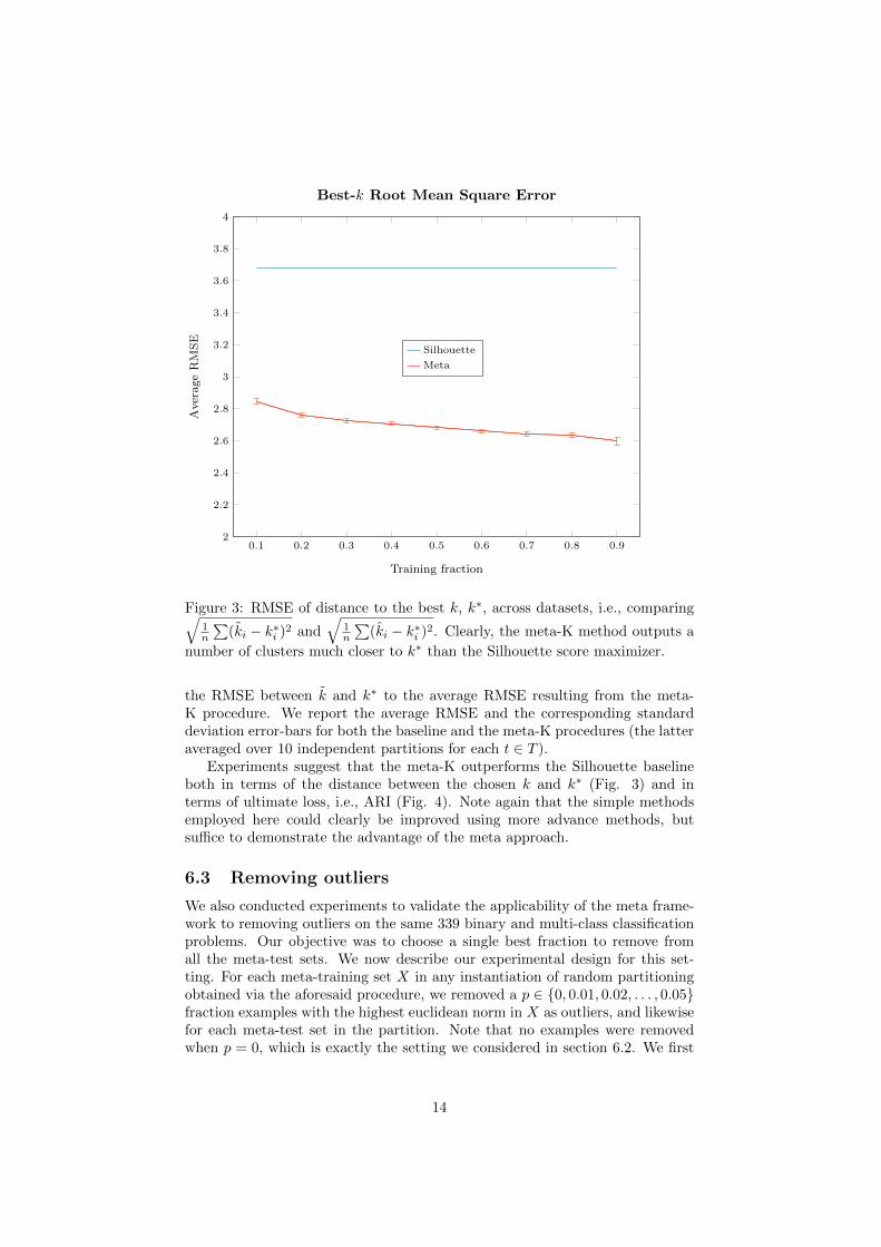
Figure 3: RMSE of distance to the best k, k∗, across datasets, i.e., comparing√1n
∑(ki − k∗i )2 and
√1n
∑(ki − k∗i )2. Clearly, the meta-K method outputs a
number of clusters much closer to k∗ than the Silhouette score maximizer.
the RMSE between k and k∗ to the average RMSE resulting from the meta-K procedure. We report the average RMSE and the corresponding standarddeviation error-bars for both the baseline and the meta-K procedures (the latteraveraged over 10 independent partitions for each t ∈ T ).
Experiments suggest that the meta-K outperforms the Silhouette baselineboth in terms of the distance between the chosen k and k∗ (Fig. 3) and interms of ultimate loss, i.e., ARI (Fig. 4). Note again that the simple methodsemployed here could clearly be improved using more advance methods, butsuffice to demonstrate the advantage of the meta approach.
6.3 Removing outliers
We also conducted experiments to validate the applicability of the meta frame-work to removing outliers on the same 339 binary and multi-class classificationproblems. Our objective was to choose a single best fraction to remove fromall the meta-test sets. We now describe our experimental design for this set-ting. For each meta-training set X in any instantiation of random partitioningobtained via the aforesaid procedure, we removed a p ∈ {0, 0.01, 0.02, . . . , 0.05}fraction examples with the highest euclidean norm in X as outliers, and likewisefor each meta-test set in the partition. Note that no examples were removedwhen p = 0, which is exactly the setting we considered in section 6.2. We first
14
0.1 0.2 0.3 0.4 0.5 0.6 0.7 0.8 0.90.08
0.09
0.1
0.11
0.12
0.13
0.14
Training fraction
Ave
rage
AR
I
Adjusted Rand Index
SilhouetteMeta
Figure 4: Average ARI scores of the meta-algorithm and the baseline for choos-ing the number of clusters, versus the fraction of problems used for training.We observe that the best k predicted by the meta approach registered a higherARI than that by Silhouette score maximizer. 95% Confidence interval obtainedwith 1000 random splits.
15
0.1 0.2 0.3 0.4 0.5 0.6 0.7 0.8 0.90.08
0.09
0.1
0.11
0.12
0.13
0.14
Training fraction
Ave
rage
Ad
just
edR
IAdjusted Rand Index (Outlier Removal)
5%
4%
3%
2%
1%
0%
Figure 5: Outlier removal results. Removing 1% of the instances as outliersimproves on the ARI scores obtained without outlier removal.
clustered the data without outliers, and obtained the corresponding Silhouettescores. We then put back the outliers by assigning them to their nearest clus-ter center, and computed the ARI score thereof. Then, following an identicalprocedure to the meta-K algorithm of section 6.2, we fitted regression modelsfor ARI corresponding to complete data using the silhouette scores on pruneddata, and measured the effect of outlier removal in terms of the true averageARI (corresponding to the best predicted ARI) over entire data. Again, wereport the results averaged over 10 independent partitions.
As shown in Fig. 5, by treating 1% of the instances in each dataset asoutliers, we achieved an improvement in ARI scores relative to clustering withall the data as in section 6.2. As the fraction of data considered outlier wasincreased to 2% or higher, however, we observed a substantial dip in the per-formance. While 1% was the optimal fraction among the candidates, clearlyfurther parameter search and improved outlier removal algorithms could pro-vide additional benefit. Our goal in this paper is mainly to pose the questionsand demonstrate that meta-learning can improve performance across problemsfrom different domains and of possibly different dimensionality.
6.4 Deep learning a binary similarity function
In this section, we consider a new unsupervised problem of learning a binarysimilarity function (BSF) that predicts whether two examples from a given
16
problem should belong to the same cluster (i.e., have the same class label).Formally, a problem is specified by a set X of data and meta-features φ. Thegoal is to learn a classifier f(x, x′, φ) ∈ {0, 1} that takes two examples x, x′ ∈ Xand the corresponding problem meta-features φ, and predicts 1 if the input pairwould belong to the same cluster (or have the same class labels). Here, weapproximate this function using a neural network.
In our experiments, we take Euclidean data X ⊆ Rd (each problem mayhave different dimensionality d) and the meta-features φ = Σ(X) consist of thecovariance matrix of the unlabeled data. We restricted our experiments to the146 datasets with at most 1000 examples and 10 features. We normalized eachdataset to have zero mean and unit variance along every coordinate. Hence thecovariance matrix was 1 on the diagonal.
We randomly sampled pairs of examples from each dataset to form meta-training and meta-test sets as described in the following section 6.4.1. For eachpair, we concatenated the features to create data with 20 features (padding ex-amples with fewer than 10 features with zeros). We then computed the empiricalcovariance matrix of the dataset, and vectorized the entries of the covariancematrix on and above the leading diagonal to obtain an additional 55 covariancefeatures. We then concatenated these features with the 20 features to form a75-dimensional feature vector per pair. Thus all pairs sampled from the samedataset shared the 55 covariance features. Moreover, we derived a new binarylabel dataset in the following way. We assigned a label 1 to pairs formed bycombining examples belonging to the same class, and 0 otherwise. In summary,each of the 146 datasets resulted in a new dataset with 75 features and binarylabels.
6.4.1 Sampling pairs to form meta-train and meta-test datasets
We formed a partition of the new datasets by randomly assigning each datasetto one of the two categories with equal probability. Each dataset in the firstcategory was used to sample data pairs for both the meta-training and themeta-internal test (meta-IT) datasets, while the second category did not con-tribute any training data and was exclusively used to generate only the meta-external test (meta-ET) dataset.
We constructed meta-training pairs by sampling randomly pairs from eachdataset in the first category. In order to mitigate the bias resulting from thevariability in size of the different datasets, we restricted the number of pairssampled from each dataset to at most 2500. Likewise, we obtained the meta-ITdataset by collecting randomly sampling each dataset subject to the maximum2500 pairs. Specifically, we randomly shuffled each dataset belonging to thefirst category, and used the first half (or 2500 examples, whichever was fewer) ofthe dataset for the meta-training data, and the following indices for the meta-IT data, again subject to maximum 2500 instances. This procedure ensureda disjoint intersection between the meta-training and the meta-IT data. Notethat combining thousands of examples from each of hundreds of problems yieldshundreds of thousands of examples, turning small data into big data. Thisprovides a means of making DNNs naturally applicable to data sets that mighthave otherwise been too small.
We created the meta-ET data using datasets belonging to the second cat-egory. Again, we sampled at most 2500 examples from each dataset in the
17
second category. We emphasize that the datasets in the second category didnot contribute any training data for our experiments.
We performed 10 independent experiments to obtain multiple partitions ofthe datasets into two categories, and repeated the aforementioned procedure toprepare 10 separate (meta-training, meta-IT, meta-ET) triplets. This resultedin the following (average size +/- standard deviation) statistics for dataset sizes:
meta-training and meta-IT : 173, 762± 10, 739
meta-ET : 172, 565± 11, 915
In order to ensure symmetry of the binary similarity function, we introducedan additional meta-training pair for each meta-training pair in the meta-trainingset: in this new pair, we swapped the order of the feature vectors of the twoinstances while replicating the covariance features of the underlying dataset thatcontributed the two instances (the covariance features, being symmetric, carriedover unchanged).
6.4.2 Training neural models
For each meta-training set, we trained an independent deep net model with4 hidden layers having 100, 50, 25, and 12 neurons respectively over just 10epochs, and used batches of size 250 each. We updated the parameters ofthe model via the Adadelta6 implementation of the stochastic gradient descent(SGD) procedure supplied with the Torch library7 with the default setting ofthe parameters, specifically, interpolation parameter equal to 0.9 and no weightdecay. We trained the model via the standard negative log-likelihood criterion(NLL). We employed ReLU non-linearity at each hidden layer but the last one,where we invoked the log-softmax function.
We tested our trained models on meta-IT and meta-ET data. For eachfeature vector in meta-IT (respectively meta-ET), we computed the predictedsame class probability. We added the predicted same class probability for thefeature vector obtained with flipped order, as described earlier for the featurevectors in the meta-training set. We predicted the instances in the correspondingpair to be in the same cluster if the average of these two probabilities exceeded0.5, otherwise we segregated them.
6.4.3 Results
We compared the meta approach to a hypothetical majority rule that had pre-science about the class distribution.8 As the name suggests, the majority rulepredicted all pairs to have the majority label, i.e., on a problem-by-problem ba-sis we determined whether 1 (same class) or 0 (different class) was more accurateand gave the baseline the advantage of this knowledge for each problem, eventhough it normally wouldn’t be available at classification time. This informationabout the distribution of the labels was not accessible to our meta-algorithm.
6described in http://arxiv.org/abs/1212.5701 .7available at: https://github.com/torch/torch7 .8Recall that we reduced the problem of clustering to pairwise binary classification, where
1 represented same cluster relations.
18
Internal test (IT) External test (ET)0.4
0.45
0.5
0.55
0.6
0.65
0.7
0.75
0.8
Ave
rage
accu
racy
Average binary similarity prediction accuracy
MetaMajority
Figure 6: Mean accuracy and standard deviation on meta-IT and meta-ETdata. Comparison between the fraction of pairs correctly predicted by the metaalgorithm and the majority rule. Recall that meta-ET, unlike meta-IT, wasgenerated from a partition that did not contribute any training data. Nonethe-less, the meta approach significantly improved upon the majority rule even onmeta-ET.
19
Fig. 6 shows the average fraction of similarity pairs correctly identified rel-ative to the corresponding pairwise ground truth relations on the two test sets,and the corresponding standard deviations across the 10 independent (meta-training, meta-IT, meta-ET) collections. Clearly, the meta approach outper-forms the majority rule on meta-IT, illustrating the benefits of the meta ap-proach in a multi-task transductive setting. More interesting, still, is the signif-icant improvement exhibited by the meta method on meta-ET, despite having itscategory precluded from contributing any data for training. The result clearlydemonstrates the benefits of leveraging archived supervised data for informeddecision making in unsupervised settings such as binary similarity prediction.
7 Conclusion
Currently, UL is difficult to define. We argue that this is because UL problemsare generally considered in isolation. We suggest that they can be viewed asrepresentative samples from some meta-distribution µ over UL problems. Weshow how a repository of multiple datasets annotated with ground truth labelscan be used to improve average performance. Theoretically, this enables us tomake UL problems, such as clustering, well-defined.
At a very high level, one could even consider the distribution of data runthrough a popular clustering toolkit, such as scikit-learn. While there is atremendous variety of problems encountered by such a group, an individualclustering course reviews may find that they are not even the first to wish tocluster course reviews using the tool.
Prior datasets may prove useful for a variety of reasons, from simple tocomplex. The prior datasets may help one choose the best clustering algorithmor parameter settings, or shared features may be transferred from prior datasetsthat can be identified as useful. We also demonstrate how the combination ofmany small data sets can form a large data set appropriate for a neural network.
This work is meant only as a first step in defining the problem of meta-unsupervised-learning. The algorithms we have introduced can surely be im-proved in numerous ways, and the experiments are mainly intended to show thatthere is potential for improving performance using a heterogeneous repositoryof prior labeled data.
References
[1] M. Ackerman and S. Ben-David. Measures of clustering quality: A workingset of axioms for clustering. In NIPS, 2008.
[2] M.-F. Balcan, A. Blum, and S. Vempala. A discriminative framework forclustering via similarity functions. In Proceedings of the Fortieth AnnualACM Symposium on Theory of Computing (STOC), pages 671–680, 2008.
[3] M.-F. Balcan, A. Blum, and S. Vempala. Efficient representations for life-long learning and autoencoding. In Workshop on Computational LearningTheory (COLT), 2015.
20
[4] H. Daume III and D. Marcu. A bayesian model for supervised clusteringwith the dirichlet process prior. Journal of Machine Learning Research(JMLR), 6:1551–1577, 2005.
[5] M. Feurer, A. Klein, K. Eggensperger, J. Springenberg, M. Blum, andF. Hutter. Efficient and robust automated machine learning. In Advancesin Neural Information Processing Systems, pages 2962–2970, 2015.
[6] T. Finley and T. Joachims. Supervised clustering with support vectormachines. In ICML, 2005.
[7] L. Hubert and P. Arabie. Comparing partitions. Journal of classification,2(1):193–218, 1985.
[8] M. J. Kearns, R. E. Schapire, and L. M. Sellie. Toward efficient agnosticlearning. Machine Learning, 17(2-3):115–141, 1994.
[9] J. Kleinberg. An impossibility theorem for clustering. Advances in neuralinformation processing systems, pages 463–470, 2003.
[10] S. J. Pan and Q. Yang. A survey on transfer learning. IEEE Transactionson Knowledge and Data Engineering (TKDE), 22:1345–1359, 2010.
[11] F. Pedregosa, G. Varoquaux, A. Gramfort, V. Michel, B. Thirion, O. Grisel,M. Blondel, P. Prettenhofer, R. Weiss, V. Dubourg, J. Vanderplas, A. Pas-sos, D. Cournapeau, M. Brucher, M. Perrot, and E. Duchesnay. Scikit-learn: Machine learning in Python. Journal of Machine Learning Research,12:2825–2830, 2011.
[12] P. J. Rousseeuw. Silhouettes: a graphical aid to the interpretation andvalidation of cluster analysis. Journal of computational and applied math-ematics, 20:53–65, 1987.
[13] O. Russakovsky, J. Deng, H. Su, J. Krause, S. Satheesh, S. Ma, Z. Huang,A. Karpathy, A. Khosla, M. Bernstein, A. C. Berg, and L. Fei-Fei. Ima-geNet Large Scale Visual Recognition Challenge. International Journal ofComputer Vision (IJCV), 115(3):211–252, 2015.
[14] M. Sahlgren. The word-space model: Using distributional analysis torepresent syntagmatic and paradigmatic relations between words in high-dimensional vector spaces. 2006.
[15] J. Snoek, H. Larochelle, and R. P. Adams. Practical bayesian optimiza-tion of machine learning algorithms. In Advances in neural informationprocessing systems, pages 2951–2959, 2012.
[16] C. Thornton, F. Hutter, H. H. Hoos, and K. Leyton-Brown. Auto-weka:Combined selection and hyperparameter optimization of classification algo-rithms. In Proceedings of the 19th ACM SIGKDD international conferenceon Knowledge discovery and data mining, pages 847–855. ACM, 2013.
[17] S. Thrun and T. M. Mitchell. Lifelong robot learning. In The biology andtechnology of intelligent autonomous agents, pages 165–196. Springer, 1995.
21
[18] S. Thrun and L. Pratt. Learning to learn. Springer Science & BusinessMedia, 2012.
[19] L. G. Valiant. A theory of the learnable. Communications of the ACM,27(11):1134–1142, 1984.
[20] R. B. Zadeh and S. Ben-David. A uniqueness theorem for clustering. InProceedings of the twenty-fifth conference on uncertainty in artificial intel-ligence, pages 639–646. AUAI Press, 2009.