Page 1
First First resultsresults of of BiosoilBiosoil in France in France
Vincent BADEAU, Renaud RABASTENS (INRA Vincent BADEAU, Renaud RABASTENS (INRA ––
Nancy)Nancy)Manuel NICOLAS, Erwin ULRICH (ONF Manuel NICOLAS, Erwin ULRICH (ONF ––
Fontainebleau)Fontainebleau)
BIOSOIL ConferenceBIOSOIL ConferenceBrussels, 9th November 2009Brussels, 9th November 2009
Page 2
First First comparisonscomparisons betweenbetween twotwo campaignscampaigns
LEVEL 1 PLOTS:
Renaud RABASTENS (Master’s
degree
–
Nancy University
–
6 months)
Floristic inventorieshomogenization
of species
names
inconsistencieschanges in floristic
composition
Soil analysesinconsistenciespotential
changes
LEVEL 2 PLOTS:
Manuel NICOLAS & Erwin ULRICH –
National Forest OfficeRENECOFOR network
Soil analyses (10 sites)
Page 3
1
12 3
4
5
1 1 247 plots247 plots2 2 152 plots152 plots3 3 27 plots27 plots4 4 60 plots60 plots5 5 86 plots86 plots
5 5 RegionalRegional
OfficesOffices
First First CampaignCampaign (1993(1993--1994)1994)ICPICP--ForestsForests
1 profile 1 profile pitpit
1 1 samplesample
/ / mandatorymandatory
layerlayerL+F / H / M01 / M12 / M24 / M46L+F / H / M01 / M12 / M24 / M46
generalgeneral informationsinformationsphysicalphysical environmentenvironment
soilsoil descriptiondescriptionfloristicfloristic descriptiondescription
dendrometricdendrometric measurementsmeasurements
573 573 levellevel
1 plots1 plots
Page 4
Field Field operationsoperations National Forest National Forest InventoryInventory557 557 visitedvisited
sites / 545 sites / 545 sampledsampled
Second Second CampaignCampaign (2006(2006--2007)2007)BIOSOILBIOSOIL
4 m8 m
6 sub-samples
1 composite sample
/ depth
(±3kg)
INRA –
Arras (analyses)
INRA –
Orléans
+ JRC(results)
400 m²
Page 5
FloristicFloristic inventoriesinventories
11stst
campaigncampaign 956 956 speciesspecies (21.5 / plot)(21.5 / plot)22ndnd
campaigncampaign 1046 1046 speciesspecies (28.5 / plot)(28.5 / plot)
1
12
3
4
5
1 1 24.1 / 28.3 24.1 / 28.3 +4.2+4.22 2 20.6 / 24.8 20.6 / 24.8 +4.1+4.13 3 23.1 / 32.4 23.1 / 32.4 +9.3+9.34 4 20.0 / 34.1 20.0 / 34.1 +14.1+14.15 5 17.0 / 30.4 17.0 / 30.4 +13.4+13.4
68%
32%
710 species
common
to both
campaign
L & K ***N ***T **R *F =
C/N **
pH & S/T = Elle
nber
g
Gég
out
Page 6
-3
-2
-1
0
1
2
3
SoilSoil analysesanalyses
ΔpHH2O
– M12(Camp_2 –
Camp_1)
Sol
s ca
lcai
res
Sol
s br
uns
Sol
s ac
ides
Sol
s po
dzol
isés
Sol
s le
ssiv
és
Sol
s hy
drom
orph
es
Sol
s al
luvi
aux
25% analyses 25% analyses withwith
||ΔΔpHpH| > 0.5| > 0.5
Page 7
1st
campaign
2nd
cam
paig
n
SoilSoil analysesanalyses
allu
hydr
less
podzacid
brun
calc
4
4.5
5
5.5
6
6.5
7
7.5
8
4 4.5 5 5.5 6 6.5 7 7.5 8
pHH2O
Page 8
NitrogenNitrogen (g/kg)(g/kg)
-9-8-7-6-5-4-3-2-1012345678
-8-7-6-5-4-3-2-1
0123456
-9-8-7-6-5-4-3-2-1012345678
0 5 10 15
-8-7-6-5-4-3-2-10123456
0 2 4 6 8 10 12
0
5
10
15
20
25
30
]-7,
-2]
]-2,
-1]
]-1,
-0.5
]
]-0.
5, -0
.1]
]-0.
1, 0
.1[
[0.1
, 0.5
[
[0.5
, 1[
[1, 2
[
[2, 5
[
0
5
10
15
20
25
30
]-8,
-2]
]-2,
-1]
]-1,
-0.5
]
]-0.
5, -0
.1]
]-0.
1, 0
.1[
[0.1
, 0.5
[
[0.5
, 1[
[1, 2
[
[2, 8
[
Δ
[N]
Δ
[N]
[N] 1st campaign
[N] 1st campaign
calc
brun
acid
podz
less
hydr
allu
v
calc
brun
acid
podz
less
hydr
allu
v
Δ
[N]
Δ
[N]
Freq
(%)
Freq
(%)M01
M12
Page 9
-50-40-30-20-10
0102030405060708090
100
-200
-150
-100
-50
0
50
100
150
0
5
10
15
20
25
]-16
0, -2
0]
]-10
, -5]
]-2.
5, 2
.5[
[5, 1
0[
[20,
85[
CarbonCarbon (g/kg)(g/kg)
calc
brun
acid
podz
less
hydr
allu
v
calc
brun
acid
podz
less
hydr
allu
vΔ
[C]
Freq
(%)
-200
-150
-100
-50
0
50
100
150
0 50 100 150 200 250
Δ
[C]
[C] 1st campaign
M01
Δ
[C]
[C] 1st campaign
0
5
10
15
20
25
30
35
40
45
50
]-20
0, -5
0]
]-50
, -30
]
]-30
, -10
]
]-10
, 10[
[10,
30[
[30,
50[
[50,
150
[
Freq
(%)
M12
Δ
[C]
-50-40-30-20-10
0102030405060708090
100
0 50 100 150 200
Page 10
Ca couche 0-10 cm
-5
0
5
10
1 2 3 44.
5 55.
5 66.
5 77.
5 88.
25 8.5 9
9.5 10 11
11.5 12 13
Ca couche 10-20 cm
-5
0
5
10
1 2 3 44.
5 55.
5 66.
5 77.
5 88.
25 8.5 9
9.5 10 11
11.5 12 13
Ca couche 20-40 cm
-5
0
5
10
1 2 3 44.
5 55.
5 66.
5 77.
5 88.
25 8.5 9
9.5 10 11
11.5 12 13
CalciumCalcium
Page 11
Mg couche 0-10 cm
-0.5
-0.3
-0.1
0.1
0.3
0.5
0.7
1 2 3 44.
5 55.
5 66.
5 77.
5 88.
25 8.5 9
9.5 10 11
11.5 12 13
Mg couche 10-20 cm
-0.5
-0.3
-0.1
0.1
0.3
0.5
0.7
1 3 4.5 5.5 6.5 7.5 8.25 9 10 11.5 13
Mg couche 20-40 cm
-0.5
-0.3
-0.1
0.1
0.3
0.5
0.7
1 3 4.5 5.5 6.5 7.5 8.25 9 10 11.5 13
MagnesiumMagnesium
Page 12
K couche 0-10 cm
-0.1
-0.05
0
0.05
0.1
0.15
0.2
1 2 3 44.
5 55.
5 66.
5 77.
5 88.
25 8.5 9
9.5 10 11
11.5 12 13
K couche 10-20 cm
-0.1
-0.05
0
0.05
0.1
0.15
0.2
1 2 3 44.
5 55.
5 66.
5 77.
5 88.
25 8.5 9
9.5 10 11
11.5 12 13
K couche 20-40 cm
-0.1
-0.05
0
0.05
0.1
0.15
0.2
1 2 3 44.
5 55.
5 66.
5 77.
5 88.
25 8.5 9
9.5 10 11
11.5 12 13
PotassiumPotassium
Page 13
ManganeseManganese
Mn couche 0-10 cm
-0.05-0.03
-0.010.01
0.030.050.07
0.09
1 3 4.5 5.5 6.5 7.5 8.25 9 10 11.5 13
Mn couche 10-20 cm
-0.05-0.03-0.010.01
0.030.050.070.09
1 2 3 44.
5 55.
5 66.
5 77.
5 88.
25 8.5 9
9.5 10 11
11.5 12 13
Mn couche 20-40 cm
-0.05-0.03-0.010.010.030.050.070.09
1 2 3 44.
5 55.
5 66.
5 77.
5 88.
25 8.5 9
9.5 10 11
11.5 12 13
Page 14
Al couche 0-10 cm
-0.5
-0.3-0.1
0.10.3
0.50.7
0.9
1 3 4.5 5.5 6.5 7.5 8.25 9 10 11.5 13
Al couche 10-20 cm
-0.5-0.3
-0.10.1
0.30.50.7
0.9
1 3 4.5 5.5 6.5 7.5 8.25 9 10 11.5 13
Al couche 20-40 cm
-0.5-0.3
-0.10.1
0.30.50.7
0.9
1 3 4.5 5.5 6.5 7.5 8.25 9 10 11.5 13
AluminiumAluminium
Page 16
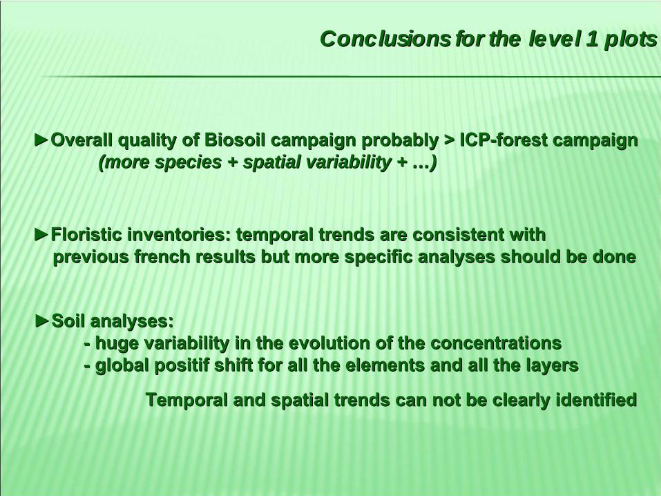
Conclusions for the Conclusions for the levellevel 1 plots1 plots
►►OverallOverall
qualityquality
of of BiosoilBiosoil
campaigncampaign
probablyprobably
> ICP> ICP--forestforest
campaigncampaign(more (more speciesspecies + spatial + spatial variabilityvariability + + ……))
►►SoilSoil
analyses:analyses:--
huge variability in the evolution of the concentrationshuge variability in the evolution of the concentrations
--
global positif shift for all the global positif shift for all the elementselements
and all the and all the layerslayers
Temporal and spatial trends Temporal and spatial trends cancan
not not bebe
clearlyclearly
identifiedidentified
►►FloristicFloristic
inventories: temporal trends are consistent inventories: temporal trends are consistent withwithpreviousprevious
french french resultsresults
but but more specific analyses should be donemore specific analyses should be done
Page 17
LevelLevel II plotsII plots
Manuel NICOLAS & Erwin ULRICHManuel NICOLAS & Erwin ULRICHRENECOFOR NetworkRENECOFOR NetworkNational Forest OfficeNational Forest Office
Page 18
1st campaign 2nd campaign
25 samples
grouped
into
5 composites
for analysis
x 3 depths
(0-10 ; 10-20 ; 20-40 cm)
Same
protocol
for both
campaigns:
G1
G2
G3
G4
G5
BiosoilBiosoil campaigncampaign –– 2007 / 2008 2007 / 2008 -- 10 plots 10 plots rere--sampledsampled11stst campaigncampaign –– 1993 / 1995 1993 / 1995 -- 102 plots 102 plots sampledsampled
Page 19
-2
-1.5
-1
-0.5
0
0.5
1
1.5
2C
PS
77
EP
C 0
8
EP
C 6
3
EP
C 8
7
HE
T 30
HE
T 64
PM
40c
PS
67a
SP
11
SP
57
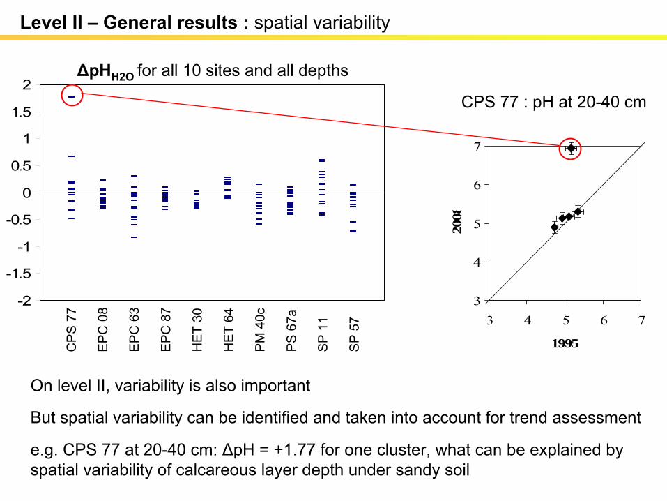
ΔpHH2O for all 10 sites and all depths
3
4
5
6
7
3 4 5 6 7
1995
2008
CPS 77 : pH at
20-40 cm
On level
II, variability
is
also
important
But spatial variability
can
be
identified
and taken
into
account
for trend assessment
e.g. CPS 77 at
20-40 cm: ΔpH = +1.77 for one cluster, what
can
be
explained
by spatial variability
of calcareous
layer depth
under
sandy
soil
Level
II –
General results
: spatial variability
Page 20
31 significant
changes (p ≤
0.05)
over 420 tests 7,4 %
0
0.5
1
1.5
2
0 0.5 1 1.5 2
1995
2008
Dashed
red
line = laboratory
detection
thresholdError
bars = laboratory
measurement
uncertainty
Example
:
[H+] graph for PS 67a plot at
0-10 cm depth
Non parametric
test (Wilcoxon
Mann Whitney for unpaired
samples) applied
in the most
conservative
case given
by uncertainties
n.s.
Level
II –
General results
: statistical
test
pH CaCl2
pH H2O Al H Ca Mg K Al+Mn+H Ca+Mg+K ECEC S/T C N C/N Sum
CPS 77 0 0 0 0 0 0 0 0 0 0 0 1 1 0 2EPC 08 0 0 0 1 0 0 0 0 0 0 0 0 0 0 1EPC 63 0 0 3 0 1 1 0 2 1 1 1 3 1 0 14EPC 87 0 0 0 1 1 1 0 0 1 0 1 1 0 0 6HET 30 0 0 0 0 0 1 0 0 1 0 0 0 0 0 2HET 64 0 0 0 0 0 0 0 0 0 0 0 0 0 0 0PM 40c 0 0 0 0 0 0 0 0 0 0 0 0 0 0 0PS 67a 0 0 0 0 0 1 1 0 0 0 0 0 0 0 2SP 11 0 0 0 0 0 1 1 0 0 0 0 0 0 0 2SP 57 0 0 0 1 0 0 1 0 0 0 0 0 0 0 2Sum 0 0 3 3 2 5 3 2 3 1 2 5 2 0 31
Exchangeable elements
Page 21
Level
II –
Results
:
No changes detected
in eutrophic/calcic
soils
(eg
HET 64)
0-10 cm
10-20 cm
20-40 cm
0
20
40
60
80
100
0 20 40 60 80 100
1995
2008
0
20
40
60
80
100
0 20 40 60 80 100
1995
2008
0
20
40
60
80
100
0 20 40 60 80 100
1995
2008
0
0.1
0.2
0.3
0.4
0 0.1 0.2 0.3 0.4
1995
2008
0
0.1
0.2
0.3
0.4
0 0.1 0.2 0.3 0.4
1995
2008
0
0.1
0.2
0.3
0.4
0 0.1 0.2 0.3 0.4
1995
2008
0
0.3
0.6
0.9
1.2
0 0.3 0.6 0.9 1.2
1995
2008
0
0.3
0.6
0.9
1.2
0 0.3 0.6 0.9 1.2
1995
2008
0
0.3
0.6
0.9
1.2
0 0.3 0.6 0.9 1.2
1995
2008
0
2
4
6
8
0 2 4 6 8
1995
2008
0
2
4
6
8
0 2 4 6 8
1995
2008
0
2
4
6
8
0 2 4 6 8
1995
2008
0
1
2
3
0 1 2 3
1995
2008
0
0.1
0.2
0.3
0.4
0.5
0 0.1 0.2 0.3 0.4 0.5
1995
2008
0
0.1
0.2
0.3
0.4
0.5
0 0.1 0.2 0.3 0.4 0.5
1995
2008
1st campaign
2ndca
mpa
ign
[Alech
] S/T[Caech
] [Mgech
] [Kech
]
Page 22
Level
II –
Results
:
Hypothetic
change to nutrient
unbalance
in acid
soils
(eg
PS 67a)
Slight
increase
of [Mg] & [K] and decrease
of [Ca] to be confirmed with further data
0-10 cm
10-20 cm
20-40 cm
0
20
40
60
80
100
0 20 40 60 80 100
1995
2008
0
20
40
60
80
100
0 20 40 60 80 100
1995
2008
0
20
40
60
80
100
0 20 40 60 80 100
1995
2008
0
0.1
0.2
0 0.1 0.2
1995
2008
+ 45 % *
0
0.1
0 0.1
1995
2008
0
0.1
0 0.1
1995
2008
0
0.1
0.2
0 0.1 0.2
1995
2008
+ 83 % *
0
0.1
0 0.1
1995
2008
0
0.1
0 0.1
1995
2008
0
0.1
0.2
0.3
0.4
0.5
0 0.1 0.2 0.3 0.4 0.5
1995
2008
0
0.1
0.2
0.3
0 0.1 0.2 0.3
1995
2008
0
0.1
0.2
0.3
0 0.1 0.2 0.3
1995
2008
0
1
2
3
4
0 1 2 3 4
1995
2008
0
1
2
3
4
0 1 2 3 4
1995
2008
0
1
2
3
4
0 1 2 3 4
1995
2008
1st campaign
2ndca
mpa
ign
[Alech
] S/T[Caech
] [Mgech
] [Kech
]
Page 23
Level
II –
Results
:
Surprising
significant
nutrient
loss
on EPC 63 plot (Andosol)
This might
be
explained
by the loss
of nutrients
inherited
from
former agricultural inputs
0-10 cm
0
20
40
60
80
100
0 20 40 60 80 100
1995
2008
0
20
40
60
80
100
0 20 40 60 80 100
1995
2008
- 57 % *
0
20
40
60
80
100
0 20 40 60 80 100
1995
2008
0
0.1
0.2
0.3
0 0.1 0.2 0.3
1995
2008
0
0.2
0.4
0.6
0.8
1
0 0.2 0.4 0.6 0.8 1
1995
2008
+ 48 % *
0
1
2
3
0 1 2 3
1995
2008
0
2
4
6
8
10
0 2 4 6 8 10
1995
2008
+ 87 % *
0
0.1
0.2
0.3
0 0.1 0.2 0.3
1995
2008
0
0.1
0.2
0.3
0 0.1 0.2 0.3
1995
2008
0
0.2
0.4
0.6
0 0.2 0.4 0.6
1995
2008
0
0.2
0.4
0.6
0 0.2 0.4 0.6
1995
2008
0
1
2
3
0 1 2 3
1995
2008
- 59 % *
0
1
2
3
4
0 1 2 3 4
1995
2008
+ 186 % *
0
1
2
3
0 1 2 3
1995
2008
0
1
2
3
4
0 1 2 3 4
1995
2008
+ 168 % *
10-20 cm
20-40 cm
2ndca
mpa
ign
1st campaign
[Alech
] S/T[Caech
] [Mgech
] [Kech
]
Page 24
Bulk
density
has increased
on 4 plots / 10 re-sampled
plots
Level
II –
Discussion on increase
of bulk
density
0
0.3
0.6
0.9
1.2
1.5
1.8
0 0.3 0.6 0.9 1.2 1.5 1.8
1995
2008
+ 17 %
0
0.3
0.6
0.9
1.2
1.5
1.8
0 0.3 0.6 0.9 1.2 1.5 1.8
1995
2008
+ 35 %
0
0.3
0.6
0.9
1.2
1.5
1.8
0 0.3 0.6 0.9 1.2 1.5 1.8
1995
2008
+ 38 %
1st campaign
2ndca
mpa
ign
10-2
0 cm
0-10
cm
20-4
0 cm
This could
be
due to soil
compaction
for 3 of them
(Norway
spruce
plantations)
E.g: EPC 08 plot
Δh = -9,6 cme1
= 10 cm
e2
= 10 cm
e3
= 20 cm
e1
’
= 8,5 cme2
’
= 7,4 cme3
’
= 14,5 cm
1993/95 2007/08
Excessive soil sampled
at
the bottom
•
Replicates
and knowledge
of harvesting
events
are necessary
to identify
the cause(s) of bulk
density
increase.
•
If soil
compaction, vertical movements
must be
integrated:
-
In the calculation
of nutrient
stocks-
In the interpretation
of concentration changes
But how the sampling method could be improved to betterintegrate management effects in long term monitoring ?
Page 25
Conclusions for the Conclusions for the levellevel 2 plots2 plots
►►
OverallOverall
qualityquality
of of BiosoilBiosoil
campaigncampaign
= 1= 1stst
campaigncampaign
►►
HighHigh
variability in the evolution of the concentrationsvariability in the evolution of the concentrationsBUTBUT
spatial spatial variabilityvariability
cancan
bebe
identifiedidentified
and and takentaken
intointo
accountaccount
Temporal trends Temporal trends cancan
bebe
identifiedidentified
►►
OnlyOnly
10 10 rere--sampledsampled
plotsplots
Temporal trends Temporal trends cancan
not not bebe
generalisedgeneralisedSpatial trends Spatial trends cancan
not not bebe
identifiedidentified