1

VIRTUAL WOODWORK: MAKING TOYS FROM GEOMETRIC MODELS

Roni Raab Center for Graphics and Geometric Computing, Dept. of Computer Science,

Technion, Haifa, Israel 32000 ronir@cs.technion.ac.il

Craig Gotsman§ Center for Graphics and Geometric Computing, Dept. of Computer Science,

Technion, Haifa, Israel 32000 gotsman@cs.technion.ac.il

http://www.cs.technion.ac.il/~gotsman

Alla Sheffer§ Center for Graphics and Geometric Computing, Dept. of Computer Science,

Technion, Haifa, Israel 32000 sheffa@cs.technion.ac.il

http://www.cs.technion.ac.il/~sheffa

Received (Day, Month, Year) Accepted (Day, Month, Year)

Shape idealization techniques provide a simplified description of a geometric model. Idealized descriptions are useful for recognition, animation, and other applications, providing a compact and efficient alternative to manipulating the complete model. Often idealized models are visually interesting in their own right and provide an appealing artistic impression of the models.

We describe an algorithm for automatic generation of idealized bead figures from recognizable 3D models (animals, humans, etc.). The bead figures approximate the model by a set of cylindrical shapes threaded onto a skeleton of the model. As such, they provide volumetric shape information in addition to the skele-ton. The bead figures can be used by applications requiring a simple and compact description of the shapes. They also provide a visually appealing, toy-like description which can be used in artistic applications. The input models are given as 3D triangulated meshes. A bead figure is generated using the skeleton of the model, often referred to as the “stick figure”. The skeleton reflects the structure of the original mesh and its features, using a small number of edges. Once the skeleton is computed, beads are threaded onto it to create the final model. Computation of a compact and concise skeleton which captures the features of the model is crucial for realistic bead figure generation.

The figure making process involves voxelization of the model; computation of the 3D Euclidean distance transform (DT); extraction of the skeleton from the DT data (combined with the model’s curvature informa-tion); and threading the beads over the skeleton.

In addition to the generation of the beaded figures, our work also introduces a novel skeleton construction algorithm. The algorithm has several advantages over existing methods and may be used in other applica-tions which utilize skeletons.

Keywords: Shape analysis, skeleton, voxelization.

2

1. Introduction

In the recent past, different application fields have showed an increasing interest in shape de-scriptions, especially for recognition purposes and design of similarity measures. Idealized or simplified descriptions are often used for shape analysis, matching [21], motion planning, ani-mation, and morphing. All of those operations are extremely cumbersome when applied to detailed polygonal models. An idealized version of the model provides a much more efficient alternative though often at the expense of accuracy.

An interesting aspect of many idealization techniques is that the resulting models are visu-ally very appealing. Skeletons remain recognizable but at the same time have an artistic, mini-malist feel, often resembling modern art-work. Non-realistic modeling and rendering is becom-ing a popular computer graphics research topic. This motivates the study of the artistic aspects of idealization in addition to the utilitarian ones.

Two main types of idealizations have been explored in depth in the literature: bounding volumes and unions of them, and skeletons. Bounding volumes [13] are useful for operations such as intersection computations and obstacle avoidance. Since they are not aimed at capturing features, they are not very suitable for other applications. For the same reason they usually do not provide a recognizable visual description.

The skeleton or medial axis of the models [2] provides a volumeless 1D or 2D idealization which captures many of the model features. They are the idealization of choice for many of the applications mentioned above. While the usefulness of skeletons has long been acknowledged, accurate and robust computation of them remains a challenging research problem. Skeletons, or stick figures, as they are often called, typically provide a good visual cue of the model shape and are useful for artistic renderings. Stick figures are easy to draw, and are an important step in creating more complex drawings. Experienced artists often begin drawing human forms by sketching their underlying structures as stick figures. Stick figures convey nicely shape infor-mation, proportions, and the relative position of different parts of an object. Stick figures have a natural extension from 2D to 3D. Instead of a drawing made up of connected 2D strokes, the model would consist of connected 3D line segments or curves (as seen in [5]), hereafter called “wire figures”. Figure 1 shows the concept of a 3D wire figure; Figure 1(a) was made of silver wire by a professional artist, and Figure 1(b) was created by a fourth grader.

The skeleton is an intrinsically volumeless description hence it lacks the notion of thick-ness which is an important visual cue in shape description. Thickness is important for such operations as intersection analysis, morphing or matching. Two models with the same skeleton can have quite different shapes. Adding the model thickness to the medial axis skeleton as sug-gested by Edelsbrunner [9] fully reproduces the shape but requires an infinite set of spheres to represent it. In this work we define an intermediate description which uses a finite number of primitives to approximate the model. The proposed description, the bead figure, consists of a set of cylindrical shapes threaded onto the skeleton. The radius of each cylinder or bead ap-proximates the medial axis transform, i.e. the model thickness at the skeleton. By providing thickness information the bead figure can be used as a much more accurate idealization of the original model. As such it can be successfully used as alternative to the skeleton. This idealiza-tion is commonly used by the toy industry (see Figures 1(c-e)). One of the advantages of such models, so-called push-toys, is the ability to control and generate nearly realistic joint motion.

The generation of bead figures which both accurately approximate the original model and are visually appealing presents several challenges as described below. In addition to developing an algorithm for generating bead figures from skeletons, this work also contributes an improved skeleton extraction algorithm. This improved algorithm was necessary to generate well-shaped bead figures but can also be used in other applications. One of the main innovations is symme-try analysis resulting in more realistic symmetric skeleton features and therefore symmetric bead figures.

3

(a)

(b)

(c)

(d)

(e)

Fig. 1. Inspiration models. (a) Wire figures of an elk, made of silver wire (by Vincent Ashworth). (b) Stick figure of a basketball player (by anonymous fourth grader). (c,d) Push toys. (e) Tinker toy.

2. Previous Work

The problem of skeleton extraction has been dealt with by many previous works, and has long been a topic of interest in both computer vision and computer graphics. The field has been widely explored in 2D, and many algorithms were extended to the 3D case. Most of the algo-rithms accept as input a discrete version of the object, such as image pixels in 2D or object voxels in 3D

In the 2D case, Costa and Estrozi [6] use label propagation which gives fairly good results. This method maintains an ordered list of pixels along the boundary of the object, and gives each of them consecutive labels (such that two adjacent border pixels have similar labels). This approach does not generalize well to the 3D case because it is impossible to impose an order on the boundary voxels (such that adjacent voxels are labeled consistently).

A standard tool in skeleton computation is the discrete distance transform. It is used to de-tect important voxels (called skeleton voxels) and connect them into a connected skeleton (e.g. [11, 12, 4, 18]). The skeleton voxels are the centers of maximal spheres (disks in the 2D case) inside the object, i.e. those which are not inscribed in any other sphere. They are often referred to as discrete medial surface (DMS) voxels. These voxels are then connected to create the re-sulting skeleton. Detecting the skeleton voxels is not straightforward, because of voxelization

4

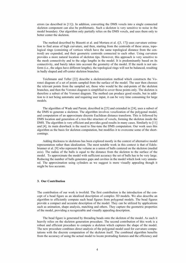
errors (as described in [11]). In addition, converting the DMS voxels into a single connected skeleton component can also be problematic. Such a skeleton is very sensitive to noise in the model boundary. Our algorithm only partially relies on the DMS voxels, and uses them only to better center the skeleton.

The method described by Biasotti et al. and Mortara et al. ([3, 17]) uses curvature estima-tion to find areas of high curvature, and then, starting from the centroids of these areas, topo-logical rings (consisting of vertices which have the same topological distance from the cen-troid) are expanded, and their geometric centroids connected to each other. Using curvature provides a more natural location of skeleton tips. However, this approach is very sensitive to the mesh connectivity and to the edge lengths in the model. It is predominantly based on its connectivity, and barely takes into account the geometry of the model. If the mesh is not uni-form (i.e., the edges have different lengths), the topological rings will not be balanced, resulting in badly shaped and off-center skeleton branches.

Teichmann and Teller [22] describe a skeletonization method which constructs the Vo-ronoi diagram of a set of points sampled from the surface of the model. The user then chooses the relevant points from the sampled set, those who would be the end-points of the skeleton branches, and then the Voronoi diagram is simplified to cover those points only. The skeleton is therefore a subset of the Voronoi diagram. The method can produce good results, but in addi-tion to it not being automatic and requiring user input, it can be very time consuming for large models.

The algorithm of Wade and Parent, described in [23] and extended in [24], uses a subset of the DMS to generate a skeleton. The algorithm involves voxelization of the polygonal model, and computation of an approximate discrete Euclidean distance transform. This is followed by DMS location and generation of a tree-like structure of voxels, forming the skeleton inside the DMS. The algorithm is very efficient and provides good results in many cases. Similarly to [11] and [4], its main drawback is the need to fine-tune the DMS computation. Our work uses this algorithm as the basis for skeleton computation, but modifies it to overcome some of the short-comings.

Adding thickness to skeletons has been explored mostly in the context of alternative model representation rather than idealization. The most notable work in this context is that of Edels-brunner et al. [9] who represent the volume as a union of balls centered on the skeleton (medial axis). The radius of the balls is equal to the distance from the skeleton to the surface of the model. To approximate the model with sufficient accuracy the set of balls has to be very large. Reducing the number of balls generates gaps and cavities in the model which look very unnatu-ral. The approximation using cylinders as we suggest is more visually appealing though it might be less accurate.

3. Our Contribution

The contribution of our work is twofold. The first contribution is the introduction of the con-cept of a bead figure as an idealized description of complex 3D models. We also describe an algorithm to efficiently compute such bead figures from polygonal models. The bead figures provide a compact and accurate description of the model. They can be utilized by applications such as animation, shape analysis, matching and others. They capture the geometric properties of the model, providing a recognizable and visually appealing description.

The bead figure is generated by threading beads onto the skeleton of the model. As such it heavily relies on the skeleton generation procedure. The second contribution of this work is a robust and efficient procedure to compute a skeleton which captures the shape of the model. The new procedure combines direct analysis of the polygonal model used for curvature compu-tations with the discrete computation of the skeleton itself. The combined algorithm benefits from the accuracy of using the actual model to locate protruding features and the efficiency and

5

robustness provided by discrete voxelization techniques. Most skeletonization algorithms do not preserve model symmetry. Due to voxelization, the loss of symmetry is especially signifi-cant when discrete algorithms are used. Symmetry is a very important property which is very noticeable to the human eye. Hence when generating both the skeletons and the subsequent bead figures it is very important to preserve it. This paper introduces a novel procedure which restores symmetry to both skeletons and subsequent bead figures.

The bead figure construction consists of the following three stages. The heart of the algo-rithm is the skeletonization procedure described in Section 4. The resulting skeleton is exam-ined for symmetries (Section 5). To generate a more realistic and visually pleasing model, symmetry is enforced even on nearly symmetric skeleton branches. Beads are threaded onto the skeleton (Section 6) to add realistic thickness to the model. Finally, the skeleton is analyzed to detect thin plate regions (Section 7), which are sometimes another important shape feature of the model.

4. Skeletonization

In order for the skeleton to correspond to the original model, the skeleton should be nicely cen-tered inside the model, and have branches that correspond to any protruding features of the model. In addition, the skeleton should be fully connected, and ideally have only a small num-ber of branches and junctions.

The skeletonization algorithm we used follows the approach of Wade and Parent [23, 24]. To improve the robustness and the quality of the results several modifications were made.

• In the original algorithm [24] the voxels paths are restricted to pass only through DMS voxels. Due to its discrete nature the DMS typically has multiple connected components. This can cause the skeletonization algorithm to fail, providing meaningless results. Even when the DMS is connected, it is often overly restrictive to require the skeleton to lie en-tirely inside it. Our algorithm does not restrict the voxel path to DMS voxels only. However, to prioritize the use of DMS voxels a path cost function (defined in Section 4.4.1) is designed to favor them . This results in a more robust computation resulting in better shaped skeletons.

• In [24], the algorithm adds branches to the skeleton one at a time, starting from locally maximal voxels (those which are locally farthest from the skeleton). This heuristic is very sensitive to the voxelization and to the state of the skeleton at that point in time. Our algo-rithm locates feature tips using curvature. Paths are then added to the skeleton, starting from farthest feature points. This procedure captures features more accurately and is less prone to discretization errors (see Figure 6).

In addition to those modifications, our new skeletonization algorithm contains a symmetry detection and restoration procedure. This procedure is necessary to compensate for loss of symmetry in the skeletons resulting from the discrete voxelization. Since the human eye is ex-tremely sensitive to (lack of) symmetry, the procedure is crucial to the generation of visually appealing bead figures.

This section describes the steps of our skeleton extraction algorithm. Section 4.1 depicts how the model is voxelized into a discrete 3D voxel world, and how the distance transform is computed. Sections 4.2 and 4.3 describe the extraction of the medial surface and the computa-tion of curvature on the model’s surface. Both these techniques are later used in the skeleton extraction algorithm, as described in Section 4.4.

6

4.1. Voxelization and the distance transform

The input to our algorithm is a 3D polygonal model. Extracting the skeleton in a 3D discrete world instead of a continuous one is faster and more robust, therefore we discretize the polygo-nal model into a set of 3D voxels. The voxelization is performed as described by Huang et al. [14] in the bounding box of the model. Each vertex, edge and face is voxelized such that the resulting voxels are 6-separated, and since they intersect the surface of the original model they are marked as surface voxels. We do not require that the polygonal input data form a single connected surface, but if it is so - the algorithm guarantees that after the voxelization process, the surface voxels also form a closed connected object. Hence each voxel can be identified as being either on the surface, inside the model or outside it. The inside/outside classification is crucial for the subsequent processing. The output of the voxelization algorithm can be seen in Figure 2.

Following the voxelization, the Euclidean distance transform of the object is computed. The distance transform at a voxel (its distance field value) is the minimum distance from the voxel to a surface voxel (the boundary of the volumetric object). It is also the radius of the sphere whose center is at the voxel, and is tangent to the boundary of the model. This is given by:

( , , )( ) min { (( , , ), ( , , )) : ( , , ) }i j kDT v d x y z i j k i j k SV= ∈

where (x,y,z) are the coordinates of the center of voxel v, SV is the set of surface voxels, and d(v1,v2) is the Euclidean distance between two voxels. We use the discrete distance transform to efficiently and robustly compute the skeleton. Various methods can be used to approximate the distance transform (e.g. [10, 15]). By using the discrete 3D distance transform computation on the voxel space, as described by Satherley and Jones [19], we compute a good approximation of the Euclidean distance transform for each voxel. The algorithm is very efficient, and gives ex-cellent, though not accurate, results. There does not seem to be a precise upper bound on the deviation. A 2D example can be seen in Figure 5.

(a)

(b)

Fig. 2. Voxelization. (a) The original horse model. (b) Voxelized version of the model (75 voxels in each di-mension)

7

4.2. Medial Surface Extraction

Our algorithm utilizes an approximate medial surface to center the skeleton inside the model. We define the discrete medial surface (DMS) to be the set of interior voxels whose distance field value is larger than that of most of their 26 neighbor voxels. Such a voxel is said to be well placed inside the model (farther from the surface than most of its neighbors). The set of medial voxels is found by simply scanning the interior voxels and comparing the distance field value at them with that of their neighbors. The subsequent skeleton computation tries to propagate the skeleton edges inside the approximate medial surface (see Figure 7(a)).

4.3. Curvature Computation

To construct a skeleton that represents the original model best, we should exploit as much in-formation about the model as we can. In our algorithm, we use information about the curvature of the surface of the model to locate the tips of the skeleton. This helps us to accurately place skeleton branches in protruding features (Figure 6). Mesh-based skeleton construction algo-rithms, such as [17], use curvature estimates for the same purpose. Attali and Lachaud [1] used curvature-like information in order to simplify a continuous skeleton. Our work is, to the best of our knowledge, the first to combine the curvature estimates with a discrete skeleton compu-tation algorithm.

We estimate the mean curvature at each vertex using the polyhedral curvature definition proposed by Dyn et al. [8]. Notice that we estimate the mean curvature and not the Gaussian curvature, because although the Gaussian curvature can detect tips (like the apex of a cone), the mean curvature can also detect creases. This is necessary for our algorithm, because creases are no less important features for us than tips.

Let M be a 3D triangle mesh consisting of a set of vertices V={vi} connected to each other by a set of edges E={ei}, forming a set of triangles T={ti}. Let v1…vn be a set of ordered neighboring vertices of vertex v (see Figure 3). We define the edges vve ii −=

r . Let

),,( 1+∆= iii vvvt be the triangle formed by the edges ier and 1+ier , and its corresponding normal is

in . The dihedral angle at an edge ier is the angle between the normals of the two triangles incident at that edge, measured in radians: ),( 1 iii nn −∠=β . S is the sum of the areas of ti. We estimate the mean curvature at a vertex v as the following quantity:

1

1 1( )4

n

i iiT

H v H eS S

β=

= = ⋅∑∫r . (2)

Curvature computation is quite sensitive even to minor noise in the input. This sensitivity can be reduced by using a wide enough neighborhood of v within a given radius. We use the vertices contained in a sphere centered at v with a given geometric radius (see Figure 4)).

Fig. 3. A vertex v and the related quantities used for curvature computation

ti

inr vi

vi-1

vi+1

1+ier

ier

1+inrβi

v

8

The steps of the complete process are:

• Identify the neighboring vertices of the vertex v within a given Euclidean distance and identify the boundary of the submesh induced by those vertices.

• Create the new "ring" of triangles connecting v with each two consecutive vertices on the submesh boundary, e.g. (v, vi, vi+1).

• Compute the mean curvature H as described above. The smaller H is, the more planar the approximating surface at the vertex v is.

• Mark feature vertices as those whose mean curvature exceeds a given threshold. Tag the voxels containing these vertices as feature voxels.

This information is used later when requiring the skeleton to pass through high curvature regions, reflecting the features of the model in the skeleton.

(a)

(b) (c)

Fig. 4. Vertex neighborhoods. (a) The 1-neighborhood of vertex v. (b) The neighborhood of vertex v within a given Euclidean radius. (c) The ring of connected triangles formed by the neighborhood boundary.

4.4. Skeleton Extraction

4.4.1. Finding the skeleton voxels

After voxelizing the model, computing the distance transform, the curvature and the medial surface information, the next (and most important) step of the algorithm is the extraction of the skeleton.

There are different methods for extracting a skeleton from the discrete 3D distance field of a model. The method we use follows the general approach described in [24]. Before we de-scribe the process, let us introduce some notation.

• Recall that a voxel’s distance field value is the radius of a sphere centered at the voxel (the sphere is tangent to the model surface). This sphere is said to cover all the voxels inside it. A skeleton voxel, therefore, covers all the voxels inside the sphere it defines (see Figure 5).

• During the skeleton extraction algorithm, paths of connected voxels are examined and as-signed two measures: the path length and the path cost.

v v v

9

• The paths are computed on the discrete voxel graph. Each voxel is connected by an edge to all of its neighbors. The length of each edge is the distance between the centers of the two voxels. Therefore, the path length is the sum of all the edge lengths along the path.

• The cost WP of a path P is

( )∑

∈ ++=

Pp iiP

i pDTpismedianW 3)()(1

1 , (3)

where DT(pi) is the distance field value at voxel pi, and ismedian(pi) is either 0 or a positive value, depending on whether the voxel pi is on the medial surface or not (if it is, the value is positive). This formula was determined empirically and gave the best results. The measure pre-fers paths which are more centered in the model (whose voxels have a higher DT value). The ismedian(pi) component magnifies the attraction of central (medial surface) voxels (see Figure 7).

The algorithm starts by first finding a heart of the model, namely, a voxel inside the model whose distance field value is maximal, i.e. it is the farthest from the object’s surface (see Figure 7(a)). The heart is not necessarily unique, and is randomly chosen in such a case.

We now compute the distance from the heart to all feature voxels using the path length measure described above. The distance is computed using the standard Dijkstra shortest path algorithm [7].

We select the feature voxel farthest from the heart, and mark it as a skeleton voxel. We also tag all the voxels it covers as covered. The skeleton is now extended in stages by the following process (see Figure 7):

1. Find the feature vertex farthest from the current skeleton which is not covered (shortest path length).

2. Find the minimal cost path from the feature voxel to the skeleton.

3. Add the path to the skeleton by marking all the voxels on the path as skeleton voxels.

4. Tag the voxels of that path as covered.

5. Update the minimal distances from the skeleton to all the voxels.

In step 1 we examine all the feature voxels. For each such voxel we have the minimal dis-tance from the voxel to the skeleton. We search for a voxel at maximal distance from the skele-ton which is not yet tagged as covered. If the distance from the voxel to the skeleton is smaller than a given threshold, the algorithm terminates. Avoiding covered voxels prevents generation of short skeleton branches. Such branches would otherwise be created in areas containing mul-tiple high curvature vertices. The termination condition also aims at preventing short branches on the skeleton. While some short branches can represent minor features it is quite typical for them to be the byproduct of approximate computations, hence usually undesirable noise.

In step 2 we find a minimal cost path from the selected feature voxel to a skeleton voxel, using a modified version of the Dijkstra algorithm. The path cost as defined above prioritizes paths farther from the surface of the model (deeper in the model) and paths which pass through DMS voxels. If more than one path has the same minimal cost, the shortest among them (in terms of path length) is chosen.

Step 3 marks all the path voxels as skeleton voxels, and step 4 marks the voxels that are covered by the newly added skeleton voxels. Finally, the minimal distance from each voxel to the updated skeleton is computed using Dijkstra’s shortest path algorithm. Notice that there is no need to update minimal distances for all skeleton voxels, and instead we can do it locally,

10

starting from the new skeleton voxels, propagating and updating voxels in the area. We con-tinue this process until all feature voxels are added, covered, or the farthest one found is already too close to the skeleton.

To emphasize the contribution of the medial surface and curvature to the skeleton computa-tion, let us study the following two cases:

• Figure 8(b) shows how the skeleton of the horse model would have looked if the medial surface (shown in Figure 8(a)) was not reflected in the path cost measure. It is evident that the skeleton is deep inside the model but is not very similar in its overall look to the origi-nal. In contrast, Figure 8(c) is the skeleton obtained when using the medial surface. It is now more similar to the original shape of the horse, since it preferred to pass through DMS voxels, which already have a shape similar to the original.

• Figure 6(a) shows how the skeleton at the legs of the triceratops model would have looked without use of curvature information (i.e., all voxels are marked as feature voxels). Notice that at the front two legs, the algorithm does not distinguish between the tips of the toes and the heels. The reason for this is that in terms of path lengths, both these areas are equi-distant from the skeleton. Hence one of the paths was randomly chosen – that originating at the heel. Figure 6(b) shows the skeleton obtained when using curvature information to de-tect that the tips of the toes are a much more curved area than the heel of the foot. As a re-sult, the skeleton at the legs originates at the tips of the toes, making it more natural.

Fig. 5. The 2D discrete distance transform for a polygon. The grey pixels are surface pixels, and every interior pixel’s value is the square of its Euclidean distance field value. A voxel is marked as skeleton voxel, and covers all voxels inside the circle defined by its distance field value (squared in this example).

(a)

(b)

Fig. 6. Contribution of curvature information. (a) Skeleton of the triceratops’ legs when no curvature information is used. (b) Skeleton when using the curvature information.

11

(a)

(b)

(c)

Fig. 8. Contribution of medial surface to skeleton computation. (a) Medial surface of the horse. (b) Skeleton without us-ing medial surface. (c) Skeleton when using the medial surface.

(a) (b)

(c) (d)

(e) (f)

Fig. 7. The steps of the skeleton extraction algorithm. (a) The original triceratops model with heart and feature areas marked. (b) The model’s medial surface. (c). The farthest feature voxel from the heart is found (the tail). The algorithm continues by connecting the point farthest from the tail (the right horn) to the tail. (d) The legs and mouth are also added. (e) The left horn is added. The remaining voxels (such as the crown) are too close to the skeleton or are already covered, so the algorithm terminates. (f) The final skeleton.

heart

12

4.4.2. Locating the structure

After all the skeleton voxels are found, the skeleton must be expressed as a tree or a list of branches. A skeleton branch starts and ends at either a junction, where it is joined to at least two other branches, or at an endpoint, where no other branch is attached to it (see Figure 9).

The branches consist of a set of connected skeleton voxels. We start with those voxels which have only one neighboring skeleton voxel, and work our way through the skeleton vox-els until we reach junctions – voxels which have at least three neighboring voxels, connecting the voxels on the way. This algorithm identifies a tree structure which contains no cycles. The initial skeleton is now complete.

Fig. 9. Endpoints and junctions of branches

4.4.3. Smoothing the skeleton

Since the skeleton computation was discrete, the branches formed might be jagged, causing the slightest change of path to be noticeable as a noncontiguous line. However, having constructed the skeleton branches, we can now easily smooth them. We apply a simple averaging filter on the branches, averaging each point on the skeleton (a voxel center) with its five neighbors (or less, when smoothing near the ends of the branch) as follows. np denotes the new position of voxel p.

1 1

4

2 11 3

2

2

;1 1;4 4

13,4... 25

n nn

j n jj j n

i

i jj i

np p np p

np p np p

i n np p

−= = −

+

= −

= =

= =

= − =

∑ ∑

∑

(4)

To further improve the skeleton, we apply a symmetry enhancing procedure (Section 5). Finally we add the beads (Section 6) and plates (Section 7).

5. Symmetry Enhancement

Symmetry is an important feature of geometric models. It is particularly noticeable in typical inputs to our methods such as animals and humans. We would like the skeleton of a model to reflect any symmetries present in the original. Symmetry in 3D models has been treated in the past, and we use notation similar to those of Zabrodsky et al. [25].

To detect symmetry, we look for nearly symmetrical branches on the skeleton. Two branches are symmetric if a plane exists in which the reflection of one branch through the plane is close to the second branch. For simplicity, we check only pairs of branches which share a junction point, and both branches start at endpoints.

Endpoints

Junctions

Endpoints

13

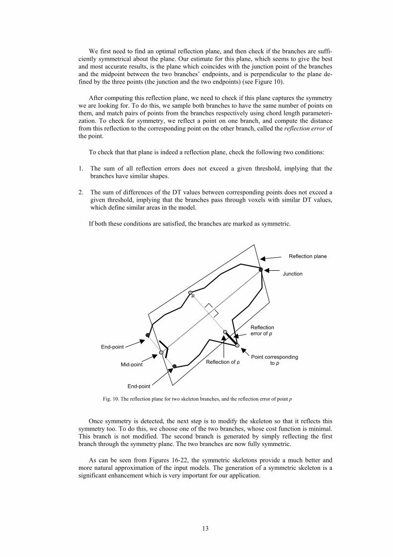
We first need to find an optimal reflection plane, and then check if the branches are suffi-ciently symmetrical about the plane. Our estimate for this plane, which seems to give the best and most accurate results, is the plane which coincides with the junction point of the branches and the midpoint between the two branches’ endpoints, and is perpendicular to the plane de-fined by the three points (the junction and the two endpoints) (see Figure 10).

After computing this reflection plane, we need to check if this plane captures the symmetry we are looking for. To do this, we sample both branches to have the same number of points on them, and match pairs of points from the branches respectively using chord length parameteri-zation. To check for symmetry, we reflect a point on one branch, and compute the distance from this reflection to the corresponding point on the other branch, called the reflection error of the point.

To check that that plane is indeed a reflection plane, check the following two conditions:

1. The sum of all reflection errors does not exceed a given threshold, implying that the branches have similar shapes.

2. The sum of differences of the DT values between corresponding points does not exceed a given threshold, implying that the branches pass through voxels with similar DT values, which define similar areas in the model.

If both these conditions are satisfied, the branches are marked as symmetric.

Fig. 10. The reflection plane for two skeleton branches, and the reflection error of point p

Once symmetry is detected, the next step is to modify the skeleton so that it reflects this

symmetry too. To do this, we choose one of the two branches, whose cost function is minimal. This branch is not modified. The second branch is generated by simply reflecting the first branch through the symmetry plane. The two branches are now fully symmetric.

As can be seen from Figures 16-22, the symmetric skeletons provide a much better and more natural approximation of the input models. The generation of a symmetric skeleton is a significant enhancement which is very important for our application.

Reflection plane

Reflection error of p

Junction

End-point

Mid-point

p

Reflection of p

End-point

Point corresponding to p

14

6. Creating the Beads

Our goal is to make wooden toy-like models. These models should have thickness and not just skeleton lines, to better visualize and resemble the original model. To achieve this look, we thread beads on the skeleton branches, as if they were made of wire.

To make them physically plausible, the beads are formed as cylinders capped with either cones or hemispheres at their ends (see Figure 12). The width (the cylinder diameter) and height (the distance between the two bases) of the beads are not fixed, and they change accord-ing to the bead’s position in the model. For the best effect, the following rules are used when designing the beads for a model.

• The radius of the bead is close to the distance field values of the voxels it is covering. It is actually an average of all the distance field values of the branch’s voxels. For example, in the model of the horse (see Figure 17) its body (the branch attaching its front and back legs) is originally wider than its legs. We want the beads threaded on its body to be thicker than those on its legs.

• There should be smooth gradation of lengths and widths of beads, in order not to have abrupt differences between adjacent beads (for example, we should avoid placing a long thin bead between two very short thick beads).

• The width of the bead should not exceed its height, so we will not have short and thick beads, rather long ones.

• Adjacent beads should not intersect one another, in order for the model to be as physically realistic as possible. Hence we "cap" the cylinders with cones or hemispheres to prevent them intersecting their neighbors (see Figure 12(d)).

• A bead should be symmetric, namely, if it is capped on one end, the other end should be capped similarly (see Figures 12(a-c))

The first step is to thread the beads. To do this, we perform the following steps for each branch. The algorithm is recursive. Later we will deal with the junctions where branches meet:

1. Try to put one bead on the entire branch, starting at one end of the branch and ending at the other. Check if the bead meets the following requirements:

• Examine all voxels on the branch and record the minimal and maximal distance field values. If the ratio between the max and min values does not exceed a given threshold, the bead is acceptable. This means that all the voxels on the branch covered by the bead are basically alike, as they all lie at similar distances from the surface.

• Verify that the skeleton is straight enough for the bead to properly express it. Other-wise, we might get one straight long bead instead of a curved branch. Scan the voxels on the branch; for each voxel compute the distance between its center and the center axis of the bead, and compare it to the distance field of the same voxel. If the ratio be-tween the distance to the axis and the distance field does not exceed a given threshold, the voxel is close enough to the bead. If at least one voxel is too far – the bead does not meet the requirement.

If the bead satisfies these two conditions, add it to the model.

2. Otherwise, split the bead in half, forming two different beads which meet at the middle of the branch (by simply counting the number of voxels from each end). Before performing the split we still need to make sure it is reasonable to do so, such that the following hold:

15

• The length of each of the two smaller beads is at least the minimal length allowed (given by the user).

• None of the two beads is shorter than its diameter.

3. When these two conditions are satisfied, it is safe to cut the bead in half, and recursively

continue the process on each of the two smaller beads.

An example of the bead-threading process can be seen in Figure 11.

(a)

(b)

(c)

(d)

(e)

Fig. 11. Bead threading. (a) The skeleton of the horse. (b) First step of recursion (for each branch) – one bead per branch. (c) Every branch except the body branch should be split in two. (d) and (e) are the next and final steps of the process. Once the basic beads have been placed, we need to cap their ends so that adjacent beads

will not intersect. To do this we compute the angle of the intersection, and "sharpen" each bead end to a cap so that the beads will touch each other only at their tips (see Figure 12(d)). The intersection computation is described below, and is defined by the height of the cone capping the cylinder (see Figure 13).

Let α be the angle between the two beads’ axes, and let r1 and r2 be the radii of the two beads. The heights of the cones capping the beads, c1 and c2 respectively, are:

1 21 2,

tan( / 2) tan( / 2)r rc cα α

= = (5)

16

Fig. 12. Symmetric beads consisting of cylinders capped with (a) cones (b) hemispheres or (c) a combination of both. (d) Adjacent beads.

(a) (b)

(c)

(d)

Fig. 13. (a) Two cylindrical beads intersecting each other. (b) Cones replace the ends of the cylinders. (c) Beads intersecting each other. (d) Beads after capping. After adjacent beads on the same branch have been dealt with, we treat the junctions. We

place spheres at the junctions, to which all other branches will be joined. The radius of the sphere is determined by the radius of the widest cylinder joined in the junction. The sphere will have that radius, and the cylinder will be joined to it in a smooth manner (see Figure 12(b)). The other beads which are, of course, less wide, will be cut so that only the tip of their cones touch the sphere, just as real beads would be attached. The reason for adding spheres in junc-tions is again to give the model more thickness. Junctions identify important locations of the model – usually a center point. Therefore, putting spheres at these locations will better empha-size them.

α/2

r1r2

α/2

c2c1

h

hh(a)

h

(b)

hh

(d)

17

The last stage is to use the symmetry information already available to make the beads on symmetric branches symmetric as well. To do this we can simply reflect one beaded branch about the reflection plane, and thus form the second branch.

7. Adding Plates

Some models cannot be adequately described by a simple set of polylines (the skeleton). Add-ing beads still does not provide an adequate solution (see Figure 18). A bird model, for exam-ple, contains wings, which would be better expressed by a planar "plate" rather than skeletal lines or cylindrical beads.

To detect planar regions in a 3D model, we look for areas of the model which are thin and almost planar. To do this we examine the skeleton. The skeleton has the structure of a tree, so each connected subgroup of branches is a subtree. To check whether a subtree can be better expressed as a plate, we compute the plane which best fits the subtree. This is done using a least squares fit of a plane to the voxels which lie on the branches of the subtree. The equation we solve in the least-squares sense is:

MX - N = 0, (6)

where M is an nx3 matrix whose rows are the coordinates of the branches’ voxels’ centers, N is an nx1 column vector of 1's, and X is a 3x1 column vector of unknowns, representing the plane normal. A solution to this least-squares problem is:

X = (MTM)-1MTN. (7)

We then check three things to confirm that the subtree is indeed planar:

1. Most of the voxels in the subtree and in the area defined by its convex hull are inside the model.

2. The distance from these voxels to the plane is small.

3. The distance from these voxels to the model surface is small.

If all three conditions are satisfied, the subtree represents a thin planar region of the model.

Note that if a tree satisfies these conditions, all of its subtrees will do so as well. Hence, the test can proceed bottom up.

We first examine all pairs of branches which start at endpoints and meet at a common junc-tion. If a pair is planar and a plate fits it, we expand the pair into a larger subtree by continually adding attached branches and re-checking if the subtree is still planar enough. When no more branches can be added to the subtree without violating the planarity, the subtree is classified as a plate.

We use only plates which are convex quadrilaterals or triangles. The plate is thin (has very small width) and is planar. Now, instead of using just a beaded skeleton, we can describe the eagle’s wings as two planar convex quadrilaterals (see Figure 18). In order for the plates to be somewhat uniform, we require that all plates be either triangles or quadrilaterals. We achieve this by computing the convex quadrilateral (or triangle) which best covers the plated area. If the initial convex hull is not a triangle or a quadrilateral, we use a greedy algorithm to remove ver-tices from the convex hull and minimize the error (see Figure 14). After the subtree has been classified as a plate and its corresponding plate computed, the subtree is replaced by the plate.

18

Finally, we give the plates a smoother look by "rounding" its corners. This is easily done by splitting each vertex on the plate into two vertices in close proximity so that the corner will seem rounder and the plate smoother (see Figure 15).

(a) (b) (c) (d) (e)

Fig. 14. A greedy algorithm for computing an approximating quadrilateral of a planar subtree. (a) The planar subtree. (b) The initial convex hull. (c)-(e) The greedy algorithm, each step removing the vertex of the convex hull which minimizes the difference from the initial hull.

(a)

(b)

Fig. 15. Rounding corners on the plate for a smoother look. (a) Plates of the eagle before the rounding. (b) Plates af-ter the rounding.

8. Experimental Results

Our algorithm results in models which can be used as a simple and compact approximation of the original. The bead figures we generate are visually very appealing and resemble push toys (see Figure 1). Figures 16-22 show the bead figures generated by the algorithm for several complex input models. Each of the resulting bead figures is recognizable and quite intuitive. The figures are very compact consisting of less than a couple of dozen beads. Yet they ap-proximate well the features and joints of the original models. The examples demonstrate the importance of the symmetry treatment procedure. All have sets of symmetric features which are detected and treated correctly by the skeleton extraction and the subsequent bead threading. The examples also show the skeletons constructed using our algorithm. The impact of symme-try treatment is demonstrated in Figures 16 (b,c). The algorithm detects and restores the sym-metry between the pairs of arms and legs of the female model, providing a more accurate ide-alization.

The importance of using the combined distance function during the skeleton construction is shown in Figure 8. Ignoring the Discrete Medial Surface when generating the path results in poor path location (Figure 8(b)). However, using only DMS voxels for the skeleton [24] is just as problematic since they are usually not connected (Figure 8(a)). Our hybrid approach, which

19

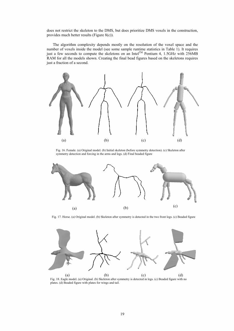
does not restrict the skeleton to the DMS, but does prioritize DMS voxels in the construction, provides much better results (Figure 8(c)).

The algorithm complexity depends mostly on the resolution of the voxel space and the number of voxels inside the model (see some sample runtime statistics in Table 1). It requires just a few seconds to compute the skeletons on an IntelTM Pentium 4, 1.5GHz with 256MB RAM for all the models shown. Creating the final bead figures based on the skeletons requires just a fraction of a second.

(a) (b) (c) (d)

Fig. 16. Female. (a) Original model. (b) Initial skeleton (before symmetry detection). (c) Skeleton after symmetry detection and forcing in the arms and legs. (d) Final beaded figure

(a)

(b) (c)

Fig. 17. Horse. (a) Original model. (b) Skeleton after symmetry is detected in the two front legs. (c) Beaded figure

(a) (b) (c) (d) Fig. 18. Eagle model. (a) Original. (b) Skeleton after symmetry is detected in legs. (c) Beaded figure with no plates. (d) Beaded figure with plates for wings and tail.

20

(a)

(b) (c)

Fig. 19. Bull. (a) Original model. (b) Skeleton after symmetry is detected in horns. (c) Beaded figure.

(a)

(b)

(c)

Fig. 20. Dinopet. (a) Original model. (b) Skeleton after symmetry is detected in legs and arms. (c) Beaded figure.

(a)

(b)

(c)

Fig. 21. Street lamp. (a) Original model. (b) Skeleton after symmetry is detected. (c) Beaded model.

21

(a)

(b)

(c)

Fig. 22. Airplane. (a) Original model. (b) Skeleton after symmetry is detected in wings and tail. (c) Beaded model.

Table 1: Algorithm runtime statistics. The last 3 columns show the runtime (in seconds) for the different stages of the skeletonization algorithm, and the percentage of that runtime of the skeleton total construction time.

Grid dimen-sions

Total voxels

Skeleton total construction

(sec)

Voxelization (sec)

Distance transform

(sec)

Skeleton extraction (sec)

Horse: 2,978 vertices, 5,952 faces

523 456,533 4.6 2.8 (61%) 0.4 (9%) 1.0 (23%)

773 140,608 11.9 5.8 (49%) 1.3 (11%) 4.4 (37%)

1023 1,061,208 27.3 10.4 (38%) 2.9 (11%) 13.6 (50%)

Female: 4,040 vertices, 8,074 faces

523 456,533 7.6 5.8 (76%) 0.4 (5%) 0.9 (12%)

773 140,608 15.2 9.5 (62%) 1.2 (8%) 4.0 (26%)

1023 1,061,208 31.1 15.6 (50%) 2.9 (9%) 12.1 (39%)

Dinopet: 2,039 vertices, 3,999 faces

523 456,533 4.2 2.4 (58%) 0.4 (10%) 1.0 (24%)

773 140,608 9.9 4.9 (50%) 1.3 (13%) 3.3 (34%)

1023 1,061,208 21.7 9.2 (42%) 2.9 (13%) 9.3 (43%)

8.1. Sensitivity analysis

Our algorithm contains some input parameters which influence the output results, such as the original mesh resolution, the voxelization resolution, the threshold for selecting feature vertices etc. We now analyze the effect of a few of the more important and influential parameters • The threshold for selecting feature vertices allows us to filter out branches caused by noise,

and keep the branches caused by “important” areas, which are more curved than others. Figure 23 shows the effect of this threshold on the skeleton of the triceratops model. In (b) the front legs are not accurate, starting from the heel instead of the toes. The best result is shown in (c). In (d) the tail is missing, caused by the threshold being too high.

22

(a)

(b)

(c)

(d)

Fig. 23. Skeleton of the triceratops model (a) using different thresholds for selecting feature vertices. (b) 50 degrees. (c) The optimal 200 degrees. (d) 300 degrees.

(a)

(b)

(c)

(d)

Fig. 24. Skeleton of the street lamp model (a) using different voxelization resolutions: (b) 753, (c) 1003, (d) 1403. • The voxelization resolution has a significant impact on the fineness and accuracy of the

skeleton. The higher the resolution, the smaller the voxels are, yielding distance transform values which are more accurate, in turn giving better results. Additionally, higher resolu-tion causes the skeleton to "dig" deeper inside the model, in smaller and more accurate steps. On the other hand, the runtime increases with resolution, as shown in Table 1. The resolution that we found to work relatively well for most of the models we experimented with is 753, but different models may require a different resolution. Figure 24 shows the in-fluence of the voxelization resolution on the skeleton of the street lamp model. Notice how the skeleton becomes more accurate in the upper extremeties in (d), when using a higher resolution. Using too low a resolution in (b) gave erroneous results in that area. The opti-mum (found by trial and error) for this model is shown in (c). Note that for this model, the optimal resolution is 1003, which is not the typical optimal resolution for most models.

23

• The choice of the size of the Euclidean neighborhood of a vertex used for curvature estima-tion can be very much model-dependent. In a model containing very sharp features (like the eagle’s claws), it would be better to choose a small neighborhood radius. In smoother models, however, in which the curved area is spread along a larger area (the horse mouth for example), it would be better to choose a wide neighborhood, in order to identify the area as curved. Notice that choosing a large radius may cause us to miss sharp features. However, choosing a radius too small may add noise to the skeleton, creating small branches to unwanted locally sharp areas. The user has to play with this parameter until the proper tradeoff is achieved. We have found that a good value is usually 1% of the maximal dimension of the model's bounding box.

• The threshold used for detecting symmetry is a distance, normalized by the model’s bound-

ing box. For a very small threshold, only branches that are almost or exactly symmetric will be recognized as such. Raising this threshold can compensate for the discretization er-ror of the skeleton, and can identify nearly symmetric branches, which were originally symmetric. However, raising the threshold too much may cause erroneous results, when identifying branches which are not symmetric at all, as symmetric. This might deform the skeleton. Figure 25 shows the skeleton of the bull model with different symmetry thresh-olds. The best result is shown in (c). In (b) a lower threshold was used, which caused the horns to be identified as asymmetric, and in (d) a higher threshold was used, causing the right hind leg and parts of the tail to be wrongly identified as symmetric, losing its original wavy shape.

(a)

(b)

(c)

(d)

Fig. 25. Skeleton of the bull model (a) using different symmetry thresholds: (b) low threshold, (c) optimal value, (d) high threshold.

Mesh resolution, in contrast to the methods proposed in [3, 17], does not have a major in-fluence on the results. In the voxelization process it does influence the runtime (as can be seen in Table 1), and can also effect the accuracy of the set of boundary voxels. The curvature com-putation and its runtime are also influenced by the resolution, but overall when looking at a neighborhood with a proper radius, the resolution does not affect the result much. Figure 26

24

shows the results on the dinopet model at three different mesh resolutions. The difference be-tween the skeletons is negligible, but the runtime increased by 50%.

(a)

(b) (c)

Fig. 26. Skeleton of the dinopet model at three resolutions: (a) low - 997 triangles, (b) medium – 3999 triangles, (c) high – 36,000 triangles.

In Figure 16(d), the female model seems to be “missing” her head, or at least the head is thinner than what would have been expected. This has a few reasons: The voxelization process, which introduces discretization errors (a higher resolution partially helps); The distance transform algorithm, which is an approximation, and may also introduce noise. The bead-splitting pa-rameter may be better tuned so that the beads will be fatter, closer to the distance transform value. This, however, will cause the rest of the figure to contain short small beads, which is undesirable. 9. Conclusion and Future Work

We have described an algorithm for creating bead figures from given a polygonal 3D model. The bead figures reflect the feature relationships inside the models, as well as volumetric in-formation and joint locations They provide a compact idealized description of the model which can be used for applications such as matching and shape analysis. Bead figures are very similar in shape to push-toys. They can be easily articulated by providing joint motion control mecha-nisms similar to those employed in push-toys. Hence bead figures are a particularly suitable idealization for motion control and animation applications. Furthermore, the resulting figures are visually very appealing and can be used for artistic design purposes.

Our algorithm for skeleton extraction is of independent interest, and can be used in areas such as shape-modeling and shape matching. It improves on other skeleton extraction algo-rithms by better reflecting the original model. This is achieved by the use of as much model information as possible – curvature points, medial surface and symmetry. This information gives the skeleton more flexibility and approximates more closely the appearance and features of the original model. The curvature computation guarantees that curved regions (or features) will be reflected in the skeleton, since the skeleton endpoints are at feature voxels. The use of the medial surface better centers the skeleton, and the symmetry restoration procedure makes the skeleton more similar to the original model.

Similarly to many other skeletonization algorithms [17, 24], our construction mechanism produces a tree-like skeleton. Therefore it will not properly express models having genus higher than zero (e.g. a torus). Detecting loops in the skeleton is not trivial [16, 20]. Future ex-tensions of our work should allow both adding loops to the skeleton and consistently threading beads onto them.

The current algorithm only guarantees that adjacent beads do not intersect one another. For applications like motion control and animation, intersections between beads from different branches should be prevented as well. An interesting topic for future work is to utilize bead models for realistic animation generation on both the idealized and original model.

25

Acknowledgments

Thanks to Mark Jones for his help with the Euclidean distance transform algorithm. The models used in this work are courtesy of Cyberware Inc., 3D Café and ocnus.com.

References

1. D. Attali and J.-O. Lachaud, Delaunay conforming iso-surface; skeleton extraction and noise

removal, Computational Geometry: Theory and Applications. 19(2-3): 175-189, 2001. 2. D. Attali and A. Montanvert, Computing and simplifying 2D and 3D continuous skeletons, Com-

puter Vision and Image Understanding, 67(3) (1997), 261-273. 3. S. Biasotti, S. Marini, M. Mortara and G. Patané, An overview on properties and efficacy of

topological skeletons in shape modelling. Shape Modeling International 2003: 245-256, 297. 4. H. Blum, A transformation for extracting new descriptors of shape, Proc. Symp. Models for the

Perception of Speech and Visual Form, ed. W. W. Dunn (MIT Press, Cambridge, MA, 1967) 362-380.

5. J. M. Cohen, Systems for sketching in 3D, Senior Thesis, Brown University (2000). 6. L. da F. Costa and L. F. Estrozi, Multidimensional scale space shape analysis, in Proc. Interna-

tional Workshop on Synthetic-Natural Hybrid Coding and Three Dimensional Imaging, Santorini, Greece (Sept. 1999) pp. 214-217,.

7. T. H. Cormen, C. E Leiserson and R. L. Rivest, Introduction to Algorithms (MIT Press, Cam-bridge, MA, YEAR).

8. N. Dyn, K. Hormann, S-J. Kim and D. Levin, Optimizing 3D triangulations using discrete curva-ture analysis, Mathematical Methods for Curves and Surfaces: Oslo 2000, eds. T. Lyche and L. Shumaker (2001) 135-146.

9. H. Edelsbrunner, The union of balls and its dual shape, in Proc. 9th Annual ACM Symposium on Computational Geometry, (1993) pp. 218-231.

10. N. Gagvani and D. Silver. Parameter controlled volume thinning, Graphical Models and Image Processing, 61(3):149-- 164, 1999.

11. Y. Ge and J. M. Fitzpatrick, On the generation of skeletons from discrete Euclidean distance maps, IEEE Transactions on Pattern Analysis and Machine Intelligence 18 (1996) 1055-1066.

12. Y. Ge and J. M. Fitzpatrick, Extraction of maximal inscribed disks from discrete Euclidean dis-tance maps, 1996 Conference on Computer Vision and Pattern Recognition (CVPR '96).

13. S. Gottschalk, M. Lin, and D. Manocha, OBBTree: A hierarchical structure for rapid interference detection, in Proc. ACM Siggraph, (1996) pp. 171–180.

14. J. Huang, R. Yagel, V. Fillipov and Y. Kurzion, An accurate method to voxelize polygonal meshes, IEEE Volume Visualization '98, Chapel Hill, NC (Oct. 1998)

15. N. Kiryati and G. Szekely, Estimating shortest paths and minimal distances on digitized three dimensional surfaces, Pattern Recognition 26 (1993) 1623-1637.

16. F. Lazarus, M. Pocchiola, G. Vegter and A. Verroust, Computing a canonical polygonal schema of an orientable triangulated surface, Seventeenth Annual ACM Symposium on Computational Geometry, Medford, MA (June 2001).

17. M. Mortara and G. Patané, Affine-invariant skeleton of 3D shapes, International Conference on Shape Modeling and Applications (SMI 2002).

18. S. M. Pizer, D. S. Fritsch, P. A. Yushkevich, V. E. Johnson, and E. L. Chaney, Segmentation, registration, and measurement of shape variation via image object shape, Transactions in Medical Imaging 18(10): 851-865 (1999).

19. R. Satherley and M. W. Jones, Vector-city vector distance transform, Computer Vision and Image Understanding 82 (2001) 238-254.

20. D. Steiner and A. Fischer, Topology recognition of 3D closed freeform objects based on topo-logical graphs, Symposium on Solid Modeling and Applications 2001, 305-306.

21. H. Sundar, D. Silver, N. Gagvani and S. Dickinson, Skeleton-based shape matching and re-trieval, in Proc. International Conference on Shape Modeling and Applications, SMI 2003, Seoul, Korea, May 2003.

22. M. Teichmann and S. Teller, Assisted articulation of closed polygonal models, in Proc. 9th Euro-graphics Workshop on Animation and Simulation, (July 1998).

23. L. Wade and R. E. Parent, Fast, fully-automated generation of control skeletons for use in anima-tion, in Proc. Computer Animation 2000, pp 189-194.

24. L. Wade and R. E. Parent, Automated generation of control skeletons for use in animation, The Visual Computer 18(2) (2002) 97-110.

25. H. Zabrodsky, S. Peleg, and D. Avnir, Symmetry as a continuous feature, IEEE Transactions on Pattern Analysis and Machine Intelligence 17 (1995), 1154-1156.