Visualizing Cells and their Connectivity Graphs for CompuCell3D

Randy Heiland∗

CREST, PervasiveTechnology InstituteIndiana University

Maciek Swat†

Biocomplexity InstituteIndiana University

James Sluka‡

Biocomplexity InstituteIndiana University

Benjamin Zaitlen§

Biocomplexity InstituteIndiana University

Abbas Shirinifard¶

Biocomplexity InstituteIndiana University

Gilberto L. Thomas‖

Instituto de FisicaUniversidade Federal do Rio

Grande do Sul

Andrew Lumsdaine∗∗

CREST, PervasiveTechnology InstituteIndiana University

James A. Glazier††

Department of Physics,Biocomplexity Institute

Indiana University

ABSTRACT

Developing models that simulate the behavior of different types ofinteracting biological cells can be a very time consuming and er-ror prone task. CompuCell3D is an open source application thataddresses this challenge. It provides interactive and customizablevisualizations that help a user detect when a model is producingthe desired behavior and when it is failing. It also allows for highquality image generation for publications and presentations. Com-puCell3D uses the Python programming language which allows foreasy extensions. Examples are provided for performing graph anal-yses of cell connectivity.

Index Terms: J.3 [Computer Applications]: Life and Medi-cal Sciences—Biology and Genetics; D.3.2 [Programming Lan-guages]: Language Classifications—Very high-level languages

1 INTRODUCTION

Developmental biology is a fascinating subject and provides signif-icant challenges for computational science. The fact that each of usbegan as a single cell and developed into trillions of cells, produc-ing a breathing, moving, thinking organism should be a source ofwonder. Many of the underlying processes for this development arenot unique to humans, however; life on this planet is, fortunately,very diverse and many developmental processes are common.

Since the discovery of the structure of DNA in the 1950s, bi-ological research has, quite understandably, been focused on themolecular level. While this has led to tremendous insights, it hasinadvertently lessened the importance of the cell as a structural unit.And yet, experimental biology is still observed at the multi-celllevel. This is where, for example, we see cells move, divide, ad-here, secrete, aggregate, communicate and die. It therefore seemslogical to conduct computational biology at a multi-cell level aswell. Sydney Brenner, a Nobel laureate in Physiology or Medicine,has stated [10]:

I believe very strongly that the fundamental unit,the correct level of abstraction, is the cell and not thegenome.

∗e-mail:heiland@indiana.edu†e-mail:maciekswat@gmail.com‡e-mail:jsluka@indiana.edu§e-mail:bzaitlen@indiana.edu¶e-mail:ashirinifard@gmail.com‖e-mail:glt@if.ufrgs.br

∗∗e-mail:lums@indiana.edu††e-mail:glazier@indiana.edu

Wolpert [14] offers a fascinating story for nonspecialists aboutthe lives of cells, explaining mitosis, growth, gastrulation, cancer,and much more.

We provide an overview of CompuCell3D (CC3D; compu-cell3d.org), a software application to simulate the behaviors of gen-eralized cells. Our focus in this paper is on the visualization ofthose cells and their connectivity with each other. CompuCell3D isprimarily used to develop models for multi-cellular biology, how-ever, it is also used for non-biological models, as we will see.

Another topic that we discuss is the Python programming lan-guage and the key role that it plays in CompuCell3D.

2 COMPUCELL3D

CC3D [8][12] is an open source software application to simulatemodels that have generalized cells as their fundamental objects.Users can download the source code and build it themselves ordownload binaries that are ready to run. The application comeswith several example models. Documentation and a community fo-rum are accessible from the web site.

All CC3D models are based on the more general Glazier-Graner-Hogeweg (GGH) mathematical model [3]. GGH is defined on auniform lattice domain and each generalized cell is a spatially de-fined contiguous subset of pixels (voxels) on the 2D (3D) lattice. A2D lattice can be either square or hexagonal (with 3D analogues).Therefore, for relatively small lattices, rendered cells can be quitepixelated. Each generalized cell shares a common cell index (σ)and is of a defined cell type (τ ). There will be very few cell typescompared to the large number of cell indices. For example, in thehuman body, while there are trillions of cells, there are on the orderof a few hundred cell types.

GGH uses an energy-based formalism to describe cell behaviors.It evolves cells using a (local) energy minimization algorithm witha Boltzmann acceptance function that simulates a constant temper-ature. The effective energy (H) is defined as follows:

H =∑

i,j

J(τ(σi), τ(σj))(1− δ(σi, σj))+

∑

σ

λvol(σ)(v(σ)− Vt(σ))2 + ... (1)

where i, j are neighbor lattice sites and σ and τ were defined above(cell index and cell type). The first sum in H calculates the adhe-sion energy between neighboring cells. Higher adhesion energiesresult in cell-cell repulsion whereas lower adhesion energies causecells to adhere. The second sum in H represents a volume conserva-tion constraint. This term will cause cells to reach a user-specifiedtarget volume and is defined in CC3D as a plugin. There are numer-ous plugins available in CC3D, each one contributing to a particularbehavior of a cell, e.g. volume, surface area, polarity, etc.. Moredetails about GGH can be found in the literature [12][11]. Mostof the code base for CC3D implements the GGH algorithm and iswritten in C++. However, Python is also used extensively.

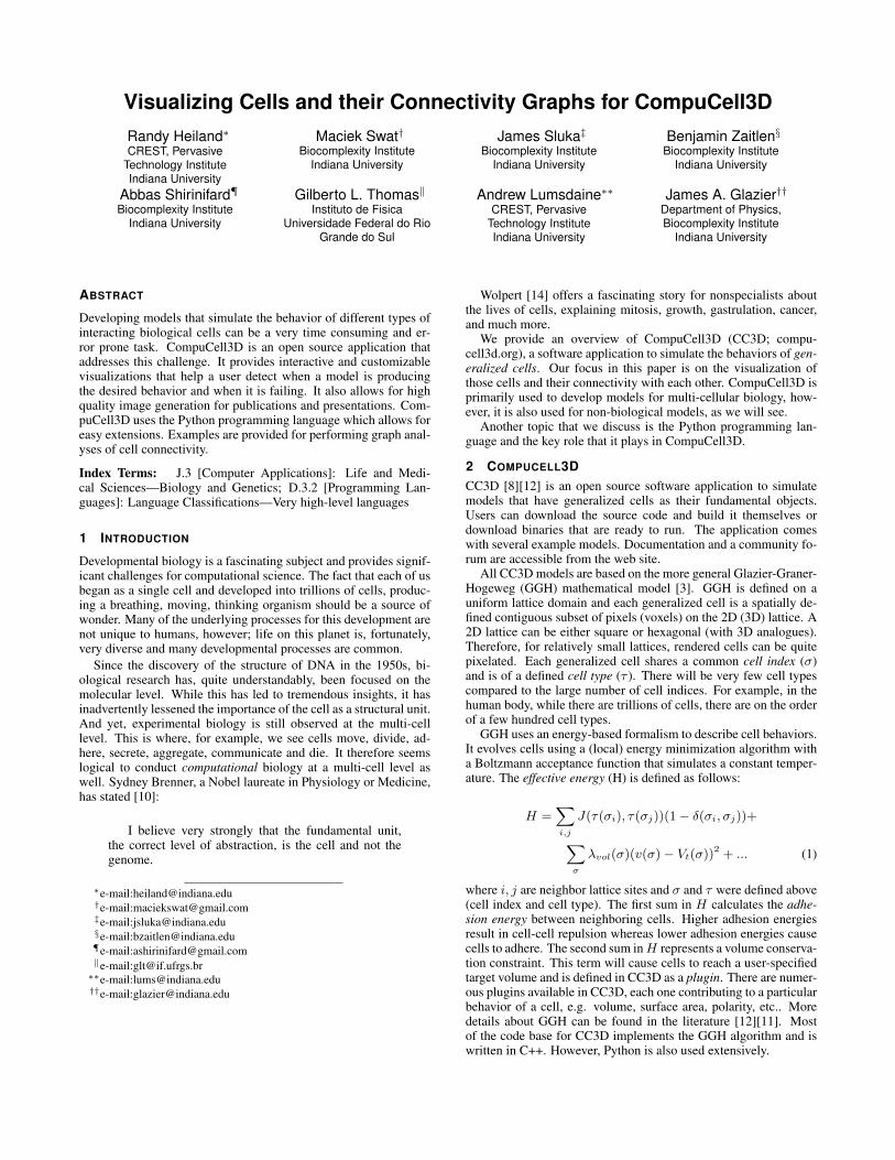
The CC3D graphical user interface (GUI) application is depictedin Figure 1. CC3D is built on an open source software stackthat includes: Python (scripting), numpy (numerics), Qt and PyQt(GUI), SWIG (wrapping C++ code in Python), and the Visualiza-tion Toolkit (VTK; also wrapped in Python). VTK is well-knownto the scientific visualization community. It uses a pipeline modelto build a visualization: data → filter → mapper → actor →

render. With dozens of filters available, there is considerable flex-ibility in creating a visualization, as we shall see.

CC3D is a multi-threaded application inside the Python inter-preter, allowing the simulation to run while a user operates the GUI.In addition to making interactive changes to the visualization, it isalso possible to steer the simulation by changing model parame-ters. Python provides a very flexible and extensible environment.Developers can rapidly prototype new ideas for visualizations, forexample. But more importantly, users can create extremely flexiblemodels by writing their own Python steppables. A Python step-pable is simply a Python module that gets executed inside the GGHalgorithm. The user can specify how frequently it is invoked duringa simulation.

In addition to providing the flexibility of writing Python step-pables that affect the model, CC3D also makes it possible for usersto write Python-wrapped VTK scripts. These will allow customvisualizations to be rendered in the GUI. Template scripts are pro-vided to help users get started, just as we provide template step-pables.

Figure 1: CC3D application.

3 EXAMPLE SIMULATIONS

We present three example simulations from CC3D. Two are of bi-ological models and the third is non-biological, but demonstratesvisualization techniques that are relevant to biology.

3.1 Cell sorting

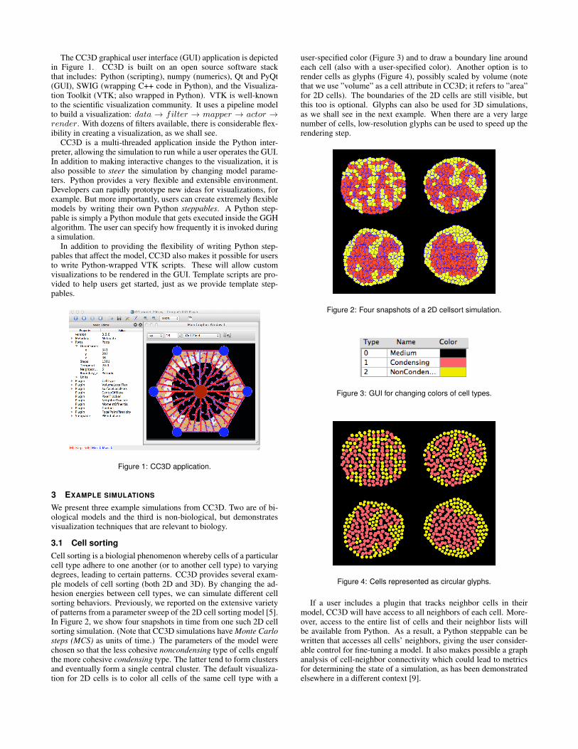
Cell sorting is a biologial phenomenon whereby cells of a particularcell type adhere to one another (or to another cell type) to varyingdegrees, leading to certain patterns. CC3D provides several exam-ple models of cell sorting (both 2D and 3D). By changing the ad-hesion energies between cell types, we can simulate different cellsorting behaviors. Previously, we reported on the extensive varietyof patterns from a parameter sweep of the 2D cell sorting model [5].In Figure 2, we show four snapshots in time from one such 2D cellsorting simulation. (Note that CC3D simulations have Monte Carlosteps (MCS) as units of time.) The parameters of the model werechosen so that the less cohesive noncondensing type of cells engulfthe more cohesive condensing type. The latter tend to form clustersand eventually form a single central cluster. The default visualiza-tion for 2D cells is to color all cells of the same cell type with a

user-specified color (Figure 3) and to draw a boundary line aroundeach cell (also with a user-specified color). Another option is torender cells as glyphs (Figure 4), possibly scaled by volume (notethat we use ”volume” as a cell attribute in CC3D; it refers to ”area”for 2D cells). The boundaries of the 2D cells are still visible, butthis too is optional. Glyphs can also be used for 3D simulations,as we shall see in the next example. When there are a very largenumber of cells, low-resolution glyphs can be used to speed up therendering step.

Figure 2: Four snapshots of a 2D cellsort simulation.

Figure 3: GUI for changing colors of cell types.

Figure 4: Cells represented as circular glyphs.

If a user includes a plugin that tracks neighbor cells in theirmodel, CC3D will have access to all neighbors of each cell. More-over, access to the entire list of cells and their neighbor lists willbe available from Python. As a result, a Python steppable can bewritten that accesses all cells’ neighbors, giving the user consider-able control for fine-tuning a model. It also makes possible a graphanalysis of cell-neighbor connectivity which could lead to metricsfor determining the state of a simulation, as has been demonstratedelsewhere in a different context [9].

To perform a graph analysis, we use NetworkX [4], an opensource Python-based software package for creating and analyzingnetworks. While not a part of CC3D proper, it demonstrates thepower of Python’s extensibility. A user can simply install Net-workX into their Python environment and thereby make it availableto a CC3D steppable. Moreover, a Python plotting package, mat-plotlib [7], can also be installed and used to easily draw graphs de-fined in NetworkX. To demonstrate, we performed a graph analysisof cell neighbors for the 2D cell sorting simulation. Some resultsfor each of the four snapshots are listed in Table 1. The connectedcomponents is perhaps the most meaningful graph measure to serveas a metric for the simulation’s state.

Figure 5 shows plots of the graphs for MCS=20 using a springlayout of the nodes. Figure 6 are plots of the same graphs, but usingthe cells’ centers of mass as positions for the nodes.

The following code snippet is from the NetworkX Python scriptthat retrieves relevant information for an undirected graph, G1, thatrepresents the neighbor connectivity for cells of a particular celltype.

G1.number_of_nodes()

G1.number_of_edges()

max(nx.degree(G1).values())

len(nx.connected_components(G1))

Figure 5: Spring layout of cell neighbors connectivity graph for con-densing (left) and noncondensing (right) cells (MCS 20).

Figure 6: Position layout (cells’ centers) of same graphs in Figure 5.

Table 1: Graph analysis for 2D cell sorting (193 cells).

Cell Type (count) MCS # edges max deg # conn comp biconnected

condensing (103)

20 196 7 3 False

1020 260 9 2 False

1960 281 9 1 False

9040 327 11 1 True

noncondensing (90)

20 117 5 9 False

1020 135 6 6 False

1960 148 7 2 False

9040 175 7 1 True

3.2 Liver lobule

The Virtual Liver is a research project of the US EnvironmentalProtection Agency that seeks to develop and test computer models

to estimate the potential of chemicals to cause chronic diseases inthe human liver [13]. The basic functional unit of the human liveris a hexagonal-shaped structure called the hepatic lobule. The lob-ule contains a large central vein, a network of blood vessels (calledsinusoids), portal venules at the vertices of the hexagon, and hepa-tocyte cells that make up the bulk of the liver mass. Each of thesecomponents have a different cell type in CC3D. Fig. 1 shows a 2Dslice during the simulation of a liver lobule model. In the model,hepatocytes (beige colored) grow in between the sinusoids from thehexagon boundary inward; hepatocytes in the process of growing(pre-mitosis) are colored white.

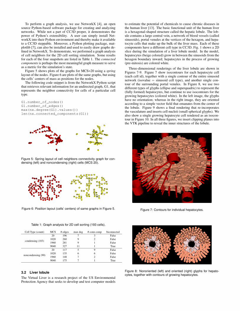
Three-dimensional renderings of the liver lobule are shown inFigures 7-9. Figure 7 show isocontours for each hepatocyte cell(each cell id), together with a single contour of the entire sinusoidnetwork (isovalue = sinusoid cell type), and another single con-tour of the surrounding portal venules. In Figure 8, we use twodifferent types of glyphs (ellipse and superquadric) to represent the(fully formed) hepatocytes, but continue to use isocontours for thegrowing hepatocytes (colored white). In the left image, the glyphshave no orientation; whereas in the right image, they are orientedaccording to a simple vector field that emanates from the center ofthe lobule. Figure 9 shows a final rendering that re-incorporatesthe vasculature and inserts cell nucleii (small spherical glyphs). Wealso show a single growing hepatocyte cell rendered as an isocon-tour in Figure 10. In all three figures, we insert clipping planes intothe VTK pipeline to reveal the inner structures of the lobule.

Figure 7: Contours for individual hepatocytes.

Figure 8: Nonoriented (left) and oriented (right) glyphs for hepato-cytes, together with contours of growing hepatocytes.

Figure 9: Liver lobule with mixture of glyphs, contours and cuttingplanes.

Figure 10: Single growing hepatocyte cell embedded in the lattice.

3.3 Foams

While the primary use of CC3D is to simulate models of cell be-havior for developmental biology, recall that the GGH algorithmoperates on generalized cells. In this example, we show resultsfrom foam simulations [1] where foam bubbles are the cells. For adry foam simulation, there is only one cell type (bubble); for wetfoams, there are two (bubble and water). Foams can undergo a pro-cess called coarsening in which some bubbles grow, others shrinkand disappear, causing the number of bubbles to decrease over time.Coarsening is also found in metallic grains and polycrystals.

CC3D provides example models for foams. Figure 11 is an im-age from a 2D dry foam simulation, showing the bubble boundariesand circular glyphs scaled by bubble area. Also shown is an imagefrom a graph analysis that highlights those bubbles (nodes) with anarea smaller than neighboring bubbles. This provides a good pre-diction of which bubbles will be eliminated.

Figure 12 shows the progression of a 3D dry foam coarseningsimulation, using semi-transparent contours of the bubbles. Fig-ure 13 depicts two different renderings of a 3D wet foam simula-tion. On the left, we contour individual bubbles (cell ids) and renderopaque surfaces. On the right, we eliminate those bubbles that in-tersect the lattice boundary and render only the interior bubbles,semi-transparently. Figure 14 show the progression of a 3D wetfoam coarsening simulation using this second technique.

4 MODEL FABRICATION

As a final example, we present a model of a 3D tumor and asurrounding vasculature network [11]. Figure 15 shows threesnapshots from the simulation. Because this model was still inits development phase, the lattice domain was relatively small(100x100x160). This created challenges for creating presentation-quality visualizations. Fortunately, VTK’s smoothing filters helped

Figure 11: 2D foam: bubble boundaries and area-scaled glyphs (left);graph analysis (right) showing nodes (red) with bubble volume lessthan each of its neighbor’s.

Figure 12: Semi-transparent renderings of 3D dry foam coarsening.

considerably. Figure 16 shows a zoom-in of the tumor’s necroticcore before smoothing and after. During the development of thismodel, we also had an opportunity to fabricate it using a 3D printer.

Fab labs [2] are, in some ways, the manufacturing analogue tothe open source software movement. Digital fabrication has be-come much more economical in recent years which has spurred agrowing interest from a variety of people – industrial designers, en-gineers, musicians, and sculptors, to name a few. Products rangefrom practical, industrial widgets to whimsical, artistic creations.Fab labs offer a variety of machines, including rapid prototypingand other 3D printers, lathes, various cutters, and more. IndianaUniversity is in the process of creating its own fab lab and we werefortunate enough to have access to a 3D printer.

Using one of VTK’s Writer objects, we were able to write astereo lithography (STL) file of the 3D tumor model. The STLmodel captured contours of cell types, with cutting planes to re-veal an inner necrotic core of the tumor (Figure 17). Since partof the vasculature was discontinuous, we needed to manually in-sert artificial (spherical) connectors into the model. Generating a3D physical model provides an interesting manipulative object todemonstrate at CC3D workshops and to use in K-12 school class-rooms and public outreach settings.

5 RELATED WORK

When considering related work to CC3D, one must distinguish be-tween the code that simulates the cells (the GGH algorithm) andthe GUI that performs the visualization. We will address only thelatter, as the former has been addressed in the literature. Since weuse VTK as our primary visualization library, it would seem rea-sonable to adopt an existing VTK-based visualization application.ParaView [6] is one such open source application, from Kitware,the same company that develops VTK. The reasons we chose todevelop our own GUI for CC3D is (1) we can customize the visual-ization choices to fit our application and (2) we need to provide syn-chronized, interactive visualizaton and co-processing for a runningsimulation. If we discover that ParaView or any other VTK-basedapplication can help meet these two criteria, we would seriouslyconsider adopting it.

Figure 13: Comparing contouring and rendering options.

Figure 14: Three snapshots of a wet foam simulation.

Figure 15: Three snapshots from the 3D tumor simulation.

Figure 16: Applying a smoothing filter to the tumor’s necrotic core.

Figure 17: Tumor model from a 3D printer.

6 CONCLUSION

We have provided an overview of CompuCell3D (CC3D), an opensource application for simulating and visualizing models of gen-eralized cells, with applications in both biology and physics. Thefact that CC3D uses the lattice-based GGH model means that cellshave the potential to be quite pixelated when visualized. A vari-ety of rendering options in CC3D, including the use of glyphs andsmoothed surfaces, have been demonstrated. CC3D uses the Visu-alization Toolkit (VTK) as its primarily visualization library. VTKoffers a simple pipeline approach for rendering data and a rich setof filters that can improve the final rendered image.

Although CC3D is written primarily in C++, we have extensivelyincorporated the Python programming language as well. In additionto the graphical user interface being in Python (PyQt), CC3D alsoprovides a mechanism for extending and fine-tuning a model viaPython steppables. A steppable can also create or modify visual-izations.

Because Python is easily extensible, we were also able to demon-strate how one could perform a graph analysis on cells’ neigh-bors connectivity using the NetworkX Python package. We believethis approach has the potential to define metrics for a simulation’sprogress and outcome.

We welcome ideas from and conversations with other researchersin both the computational biology and visualization communities.

ACKNOWLEDGEMENTS

The authors gratefully acknowledge support from the National In-stitutes of Health, National Institute of General Medical Sciencesgrants R01 GM077138 and R01 GM076692, the EnvironmentalProtection Agency grant R835001, the Lilly Endowment Inc. andthe Biocomplexity Institute at Indiana University. Indiana Univer-sitys Research Technologies (RT/UITS), provided time and assis-tance with BigRed and Quarry clusters for simulations. The Ad-vanced Visualization Lab in RT helped generate the tumor modelon their 3D printer. Early versions of CompuCell3D were devel-oped at the University of Notre Dame by JAG, Dr. Mark Alber, Dr.Jesus Izaguirre, Joseph Coffland, and collaborators with the supportof National Science Foundation, Division of Integrative Biology,grant IBN-00836563. Other developers (current and past) from In-diana University include Mitja Hmeljak, Chris Mueller and AlexDementsov. We wish to thank all the open source software commu-nities who have provided a foundation for CC3D and for the resultsin this paper: Python, numpy, IPython, VTK, NetworkX and mat-plotlib. Thanks also to Nick Edmonds and Clayton Davis for usefuldiscussions about graphs. Most of all, we thank the communityof CC3D modelers who have been our collaborators throughout itsdevelopment.

REFERENCES

[1] I. Fortuna, G. L. Thomas, R. M. C. de Almeida, and F. Graner. Growth

laws and self-similar growth regimes of coarsening two-dimensional

foams: Transition from dry to wet limits. ArXiv e-prints, Mar. 2012.

[2] N. Gershenfeld. Fab: The Coming Revolution on Your Desktop–from

Personal Computers to Personal Fabrication. Basic Books, 2005.

[3] F. Graner and J. A. Glazier. Simulation of biological cell sorting using

a two-dimensional extended potts model. Phys. Rev. Lett., 69:2013–

2016, Sep 1992.

[4] A. A. Hagberg, D. A. Schult, and P. J. Swart. Exploring network

structure, dynamics, and function using NetworkX. In Proceedings

of the 7th Python in Science Conference (SciPy2008), pages 11–15,

Pasadena, CA USA, Aug. 2008.

[5] R. Heiland, M. Swat, B. Zaitlen, J. Glazier, and A. Lumsdaine. Work-

flows for parameter studies of multi-cell modeling. In Proceedings

of the 2010 Spring Simulation Multiconference, SpringSim ’10, pages

94:1–94:6, San Diego, CA, USA, 2010. Society for Computer Simu-

lation International.

[6] A. Henderson. ParaView Guide, A Parallel Visualization Application.

Kitware Inc., 2007.

[7] J. D. Hunter. Matplotlib: A 2d graphics environment. Computing In

Science & Engineering, 9(3):90–95, May-Jun 2007.

[8] J. A. Izaguirre, R. Chaturvedi, C. Huang, T. M. Cickovski, J. Coffland,

G. Thomas, G. Forgacs, M. S. Alber, G. Hentschel, S. A. Newman,

and J. A. Glazier. Compucell, a multi-model framework for simulation

of morphogenesis. Bioinformatics, pages 1129–1137, 2004.

[9] L. McKeen-Polizzotti, K. M. Henderson, B. Oztan, C. C. Bilgin,

B. Yener, and G. E. Plopper. Quantitative metric profiles capture three-

dimensional temporospatial architecture to discriminate cellular func-

tional states. BMC Med Imaging, 11:11, 2011.

[10] D. Noble. The Music of Life: Biology Beyond Genes. Oxford Univer-

sity Press, 2008.

[11] A. Shirinifard, J. S. Gens, B. L. Zaitlen, N. J. Popawski, M. Swat, and

J. A. Glazier. 3d multi-cell simulation of tumor growth and angiogen-

esis. PLoS ONE, 4(10):e7190, 10 2009.

[12] M. H. Swat, S. D. Hester, A. I. Balter, R. W. Heiland, B. L. Zaitlen,

and J. A. Glazier. Multicell simulations of development and disease

using the CompuCell3D simulation environment. Methods Mol. Biol.,

500:361–428, 2009.

[13] J. Wambaugh and I. Shah. Simulating microdosimetry in a virtual

hepatic lobule. PLoS Comput Biol, 6(4):e1000756, 04 2010.

[14] L. Wolpert. How we live and why we die: the secret lives of cells.

Faber and Faber, 2009.