Viterbi Decoding Techniques for the TMS320C55x DSP ... · PDF fileSPRA776A Viterbi Decoding...

Application ReportSPRA776A - April 2009

1

Viterbi Decoding Techniques for the TMS320C55xDSP Generation

Henry Hendrix Member, Group Technical Staff

ABSTRACT

In most wireless communications systems, convolutional coding is the preferred method oferror-correction coding to overcome transmission distortions. This report outlines the theoryof convolutional coding and decoding, and explains the programming techniques for Viterbidecoding in the Texas Instruments TMS320C55x generation of digital signal processors(DSPs). The same basic methods decode any convolutional code. This application reportexamines the problem from a generic viewpoint rather than outlining a solution for a specificstandard.

Project collateral and source code discussed in this application report can be downloadedfrom the following URL: http://www-s.ti.com/sc/techlit/spra776.zip.

Contents

1 Introduction 2. . . . . . . . . . . . . . . . . . . . . . . . . . . . . . . . . . . . . . . . . . . . . . . . . . . . . . . . . . . . . . . . . . . . . . . . . 2 Convolutional Encoding and Viterbi Decoding 2. . . . . . . . . . . . . . . . . . . . . . . . . . . . . . . . . . . . . . . . .

2.1 Convolutional Versus Block-Level Coding 2. . . . . . . . . . . . . . . . . . . . . . . . . . . . . . . . . . . . . . . . . . . . 2.2 Encoding Process 3. . . . . . . . . . . . . . . . . . . . . . . . . . . . . . . . . . . . . . . . . . . . . . . . . . . . . . . . . . . . . . . . 2.3 Coding Rate 3. . . . . . . . . . . . . . . . . . . . . . . . . . . . . . . . . . . . . . . . . . . . . . . . . . . . . . . . . . . . . . . . . . . . . 2.4 Decoding Process 4. . . . . . . . . . . . . . . . . . . . . . . . . . . . . . . . . . . . . . . . . . . . . . . . . . . . . . . . . . . . . . . . 2.5 VA and Trellis Paths 5. . . . . . . . . . . . . . . . . . . . . . . . . . . . . . . . . . . . . . . . . . . . . . . . . . . . . . . . . . . . . . 2.6 Metric Update 6. . . . . . . . . . . . . . . . . . . . . . . . . . . . . . . . . . . . . . . . . . . . . . . . . . . . . . . . . . . . . . . . . . . . 2.7 Traceback 6. . . . . . . . . . . . . . . . . . . . . . . . . . . . . . . . . . . . . . . . . . . . . . . . . . . . . . . . . . . . . . . . . . . . . . . 2.8 Soft Versus Hard Decisions 7. . . . . . . . . . . . . . . . . . . . . . . . . . . . . . . . . . . . . . . . . . . . . . . . . . . . . . . . 2.9 Local-Distance Calculation 7. . . . . . . . . . . . . . . . . . . . . . . . . . . . . . . . . . . . . . . . . . . . . . . . . . . . . . . . . 2.10 Puncturing 8. . . . . . . . . . . . . . . . . . . . . . . . . . . . . . . . . . . . . . . . . . . . . . . . . . . . . . . . . . . . . . . . . . . . . . .

3 TMS320C55x Code for Viterbi Decoding 9. . . . . . . . . . . . . . . . . . . . . . . . . . . . . . . . . . . . . . . . . . . . . . . 3.1 Initialization 9. . . . . . . . . . . . . . . . . . . . . . . . . . . . . . . . . . . . . . . . . . . . . . . . . . . . . . . . . . . . . . . . . . . . . . 3.2 Metric Update 10. . . . . . . . . . . . . . . . . . . . . . . . . . . . . . . . . . . . . . . . . . . . . . . . . . . . . . . . . . . . . . . . . . . 3.3 Symmetry for Simplification 11. . . . . . . . . . . . . . . . . . . . . . . . . . . . . . . . . . . . . . . . . . . . . . . . . . . . . . . 3.4 Use of Buffers 12. . . . . . . . . . . . . . . . . . . . . . . . . . . . . . . . . . . . . . . . . . . . . . . . . . . . . . . . . . . . . . . . . . . 3.5 Example Metric Update 12. . . . . . . . . . . . . . . . . . . . . . . . . . . . . . . . . . . . . . . . . . . . . . . . . . . . . . . . . . 3.6 Traceback Function 16. . . . . . . . . . . . . . . . . . . . . . . . . . . . . . . . . . . . . . . . . . . . . . . . . . . . . . . . . . . . . . 3.7 Benchmarks 18. . . . . . . . . . . . . . . . . . . . . . . . . . . . . . . . . . . . . . . . . . . . . . . . . . . . . . . . . . . . . . . . . . . . 3.8 Variations in Processing 19. . . . . . . . . . . . . . . . . . . . . . . . . . . . . . . . . . . . . . . . . . . . . . . . . . . . . . . . . .

4 Convolutional Encoding on the TMS320C55x 19. . . . . . . . . . . . . . . . . . . . . . . . . . . . . . . . . . . . . . . . . 4.1 General Procedure 19. . . . . . . . . . . . . . . . . . . . . . . . . . . . . . . . . . . . . . . . . . . . . . . . . . . . . . . . . . . . . .

TMS320C55x is a trademark of Texas Instruments.

All trademarks are the property of their respective owners.

SPRA776A

2 Viterbi Decoding Techniques for the TMS320C55x DSP Generation

4.2 Benchmarks 20. . . . . . . . . . . . . . . . . . . . . . . . . . . . . . . . . . . . . . . . . . . . . . . . . . . . . . . . . . . . . . . . . . . . 5 Conclusion 21. . . . . . . . . . . . . . . . . . . . . . . . . . . . . . . . . . . . . . . . . . . . . . . . . . . . . . . . . . . . . . . . . . . . . . . . . 6 References 21. . . . . . . . . . . . . . . . . . . . . . . . . . . . . . . . . . . . . . . . . . . . . . . . . . . . . . . . . . . . . . . . . . . . . . . . . 7 Bibliography 21. . . . . . . . . . . . . . . . . . . . . . . . . . . . . . . . . . . . . . . . . . . . . . . . . . . . . . . . . . . . . . . . . . . . . . . Appendix A Viterbi API 22. . . . . . . . . . . . . . . . . . . . . . . . . . . . . . . . . . . . . . . . . . . . . . . . . . . . . . . . . . . . . . . . . Appendix B Glossary 26. . . . . . . . . . . . . . . . . . . . . . . . . . . . . . . . . . . . . . . . . . . . . . . . . . . . . . . . . . . . . . . . . .

List of Figures

Figure 1. Constraint Length 5, Rate 1/2 Convolutional Encoder 3. . . . . . . . . . . . . . . . . . . . . . . . . . . . . . . . . Figure 2. Trellis Diagram for K = 3, Rate 1/2 Convolutional Encoder 4. . . . . . . . . . . . . . . . . . . . . . . . . . . . . Figure 3. Pseudo Code for the Viterbi Algorithm 5. . . . . . . . . . . . . . . . . . . . . . . . . . . . . . . . . . . . . . . . . . . . . . Figure 4. Butterfly Structure for K = 3, Rate 1/2 Convolutional Encoder 11. . . . . . . . . . . . . . . . . . . . . . . . . Figure 5. State Variable Representation 17. . . . . . . . . . . . . . . . . . . . . . . . . . . . . . . . . . . . . . . . . . . . . . . . . . . . Figure 6. Data Rates for Overall System 18. . . . . . . . . . . . . . . . . . . . . . . . . . . . . . . . . . . . . . . . . . . . . . . . . . . .

List of Tables

Table 1. Soft-Decision Values 7. . . . . . . . . . . . . . . . . . . . . . . . . . . . . . . . . . . . . . . . . . . . . . . . . . . . . . . . . . . . . . Table 2. Local-Distance Values 8. . . . . . . . . . . . . . . . . . . . . . . . . . . . . . . . . . . . . . . . . . . . . . . . . . . . . . . . . . . . . Table 3. Metric-Update Operations for GSM Viterbi Decoding 13. . . . . . . . . . . . . . . . . . . . . . . . . . . . . . . . . . Table 4. State Ordering in Transition Data for One Symbol Interval 16. . . . . . . . . . . . . . . . . . . . . . . . . . . . Table 5. State Ordering in Transition Table for K = 6, Rate 1/2 System 16. . . . . . . . . . . . . . . . . . . . . . . . . . Table 6. Viterbi Decoding Benchmarks for Various Wireless Standards 19. . . . . . . . . . . . . . . . . . . . . . . . . .

List of Examples

Example 1. Main Loop of the GSM Viterbi Implementation 14. . . . . . . . . . . . . . . . . . . . . . . . . . . . . . . . .

1 Introduction

Although used to describe the entire error-correction process, Viterbi specifically indicates use ofthe Viterbi algorithm (VA) for decoding. The encoding method is referred to as convolutionalcoding or trellis-coded modulation. The outputs are generated by convolving a signal with itself,which adds a level of dependence on past values. A state diagram illustrating the sequence ofpossible codes creates a constrained structure called a trellis. The coded data is usuallymodulated; hence, the name trellis-coded modulation.(1)

2 Convolutional Encoding and Viterbi Decoding

2.1 Convolutional Versus Block-Level Coding

Convolutional coding is a bit-level encoding technique rather than block-level techniques suchas Reed-Solomon coding. Advantages of convolutional codes over block-level codes fortelecom/datacom applications are:(2)

• With soft-decision data, convolutionally encoded system gain degrades gracefully as theerror rate increases. Block-level codes correct errors up to a point, after which the gain dropsoff rapidly.

• Convolutional codes are decoded after an arbitrary length of data, while block-level codesintroduce latency by requiring reception of an entire data block before decoding begins.

SPRA776A


• Convolutional codes do not require block synchronization.

Although bit-level codes do not allow reconstruction of burst errors like block-level codes,interleaving techniques spread out burst errors to make them correctable.

Convolutional codes are decoded by using the trellis to find the most likely sequence of codes.The VA simplifies the decoding task by limiting the number of sequences examined. The mostlikely path to each state is retained for each new symbol.

2.2 Encoding Process

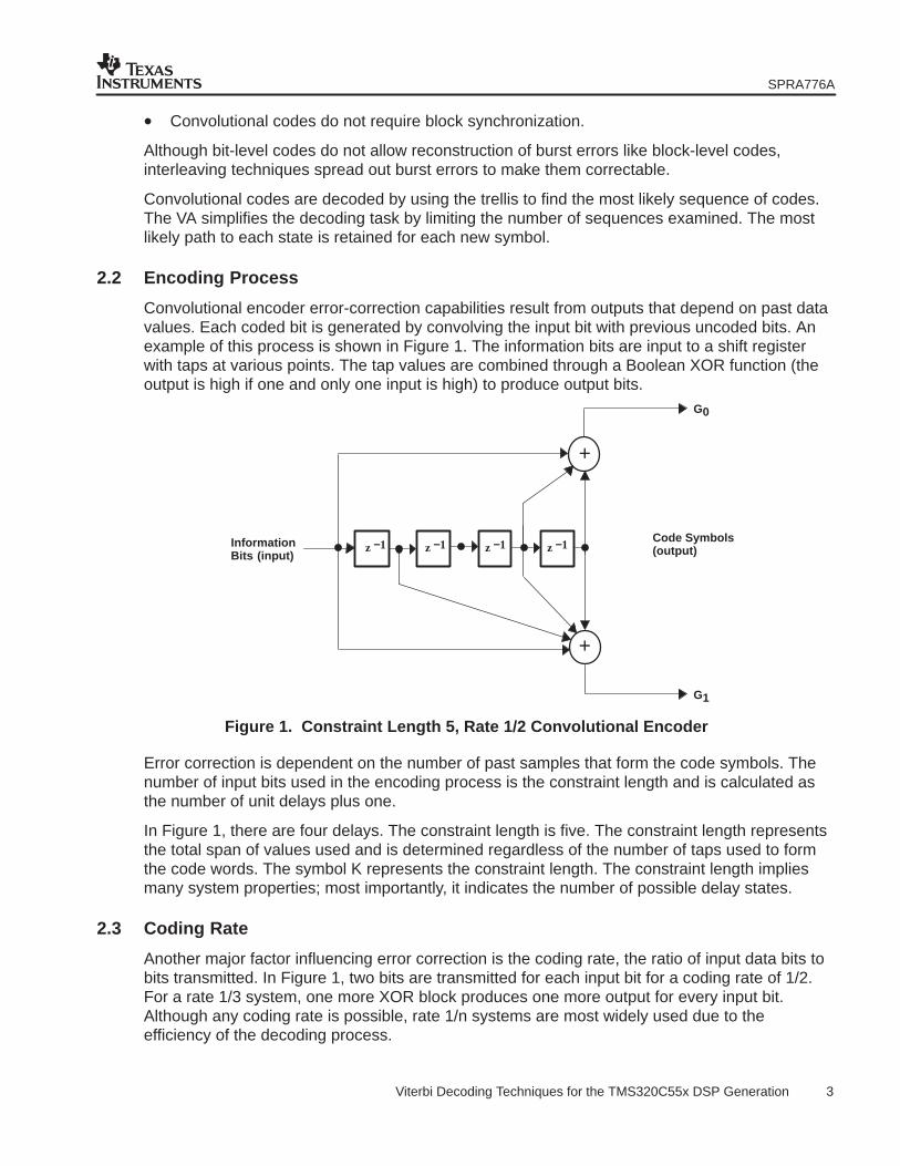
Convolutional encoder error-correction capabilities result from outputs that depend on past datavalues. Each coded bit is generated by convolving the input bit with previous uncoded bits. Anexample of this process is shown in Figure 1. The information bits are input to a shift registerwith taps at various points. The tap values are combined through a Boolean XOR function (theoutput is high if one and only one input is high) to produce output bits.

z −1InformationBits (input)

G0

G1

+

+

z −1 z −1 z −1Code Symbols(output)

Figure 1. Constraint Length 5, Rate 1/2 Convolutional Encoder

Error correction is dependent on the number of past samples that form the code symbols. Thenumber of input bits used in the encoding process is the constraint length and is calculated asthe number of unit delays plus one.

In Figure 1, there are four delays. The constraint length is five. The constraint length representsthe total span of values used and is determined regardless of the number of taps used to formthe code words. The symbol K represents the constraint length. The constraint length impliesmany system properties; most importantly, it indicates the number of possible delay states.

2.3 Coding Rate

Another major factor influencing error correction is the coding rate, the ratio of input data bits tobits transmitted. In Figure 1, two bits are transmitted for each input bit for a coding rate of 1/2.For a rate 1/3 system, one more XOR block produces one more output for every input bit.Although any coding rate is possible, rate 1/n systems are most widely used due to theefficiency of the decoding process.

SPRA776A


The output-bit combination is described by a polynomial. The system, as shown in Figure 1,uses the polynomials:

G0(x) � 1 � x3� x4

G1(x) � 1 � x � x3� x4

Polynomial selection is important because each polynomial has different error-correctingproperties. Selecting polynomials that provide the highest degree of orthogonality maximizes theprobability of finding the correct sequence.(4)

2.4 Decoding Process

Convolutionally encoded data is decoded through knowledge of the possible state transitions,created from the dependence of the current symbol on past data. The allowable state transitionsare represented by a trellis diagram.

A trellis diagram for a K = 3, 1/2-rate encoder is shown in Figure 2. The delay states representthe state of the encoder (the actual bits in the encoder shift register), while the path statesrepresent the symbols that are output from the encoder. Each column of delay states indicatesone symbol interval.

Input = 1

Input = 0

SymbolTime 0

SymbolTime 1

SymbolTime 3

SymbolTime 4

Time

Delay States

Path States G0 G1

00

11

00

11

10

01

00

11

11

00

10

01

01

10 10

01

01

10

00

11

11

0000

01

10

11

SymbolTime 2

Figure 2. Trellis Diagram for K = 3, Rate 1/2 Convolutional Encoder

The number of delay states is determined by the constraint length. In this example, theconstraint length is three, and the number of possible states is 2K−1 = 22 = 4. Knowledge of thedelay states is very useful in data decoding, but the path states are the actual encoded andtransmitted values.

(1)

(2)

SPRA776A


The number of bits representing the path states is a function of the coding rate. In this example,two output bits are generated for every input bit, resulting in 2-bit path states. A rate 1/3 (or 2/3)encoder has 3-bit path states, rate 1/4 has 4-bit path states, and so forth. Since path statesrepresent the actual transmitted values, they correspond to constellation points, the specificmagnitude and phase values used by the modulator.

The decoding process estimates the delay state sequence, based on received data symbols, toreconstruct a path through the trellis. The delay states directly represent encoded data, since thestates correspond to bits in the encoder shift register.

In Figure 2, the most significant bit (MSB) of the delay states corresponds to the most recentinput, and the least significant bit (LSB) corresponds to the previous input. Each input shifts thestate value one bit to the right, with the new bit shifting into the MSB position. For example, if thecurrent state is 00 and a 1 is input, the next state is 10; a 0 input produces a next state of 00.

Systems of all constraint lengths use similar state mapping. The correspondence between datavalues and states allows easy data reconstruction, once the path through the trellis isdetermined.

2.5 VA and Trellis Paths

The VA provides a method for minimizing the number of data-symbol sequences (trellis paths).As a maximum-likelihood decoder, the VA identifies the code sequence with the highestprobability of matching the transmitted sequence based on the received sequence.

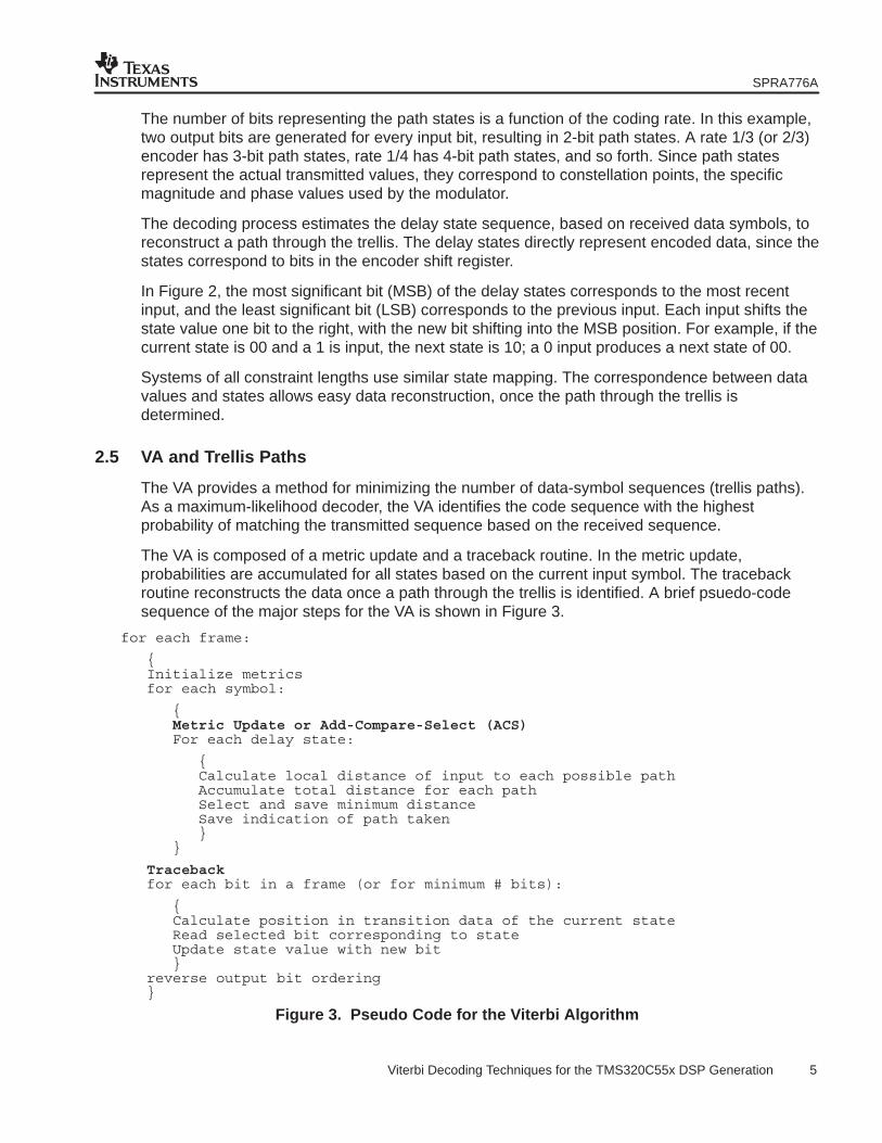
The VA is composed of a metric update and a traceback routine. In the metric update,probabilities are accumulated for all states based on the current input symbol. The tracebackroutine reconstructs the data once a path through the trellis is identified. A brief psuedo-codesequence of the major steps for the VA is shown in Figure 3.

for each frame:

{Initialize metricsfor each symbol:

{Metric Update or Add-Compare-Select (ACS)For each delay state:

{Calculate local distance of input to each possible path Accumulate total distance for each pathSelect and save minimum distance Save indication of path taken}

}

Tracebackfor each bit in a frame (or for minimum # bits):

{Calculate position in transition data of the current stateRead selected bit corresponding to stateUpdate state value with new bit}

reverse output bit ordering }

Figure 3. Pseudo Code for the Viterbi Algorithm

SPRA776A


2.6 Metric Update

Although one state is entered for each symbol transmitted, the VA must calculate the most likelyprevious state for all possible states, since the actual encoder state is not known until a numberof symbols is received. Each delay state is linked to the previous states by a subset of allpossible paths. For rate 1/n encoders, there are only two paths from each delay state. Thisconsiderably limits the calculations.

The path state is estimated by combining the current input value and the accumulated metrics ofprevious states. Since each path has an associated symbol (or constellation point), the localdistance to that symbol from the current input is calculated. For a better estimation of datavalidity, the local distance is added to the accumulated distances of the state to which the pathpoints.

Because each state has two or more possible input paths, the accumulated distance iscalculated for each input path. The path with the minimum accumulated distance is selected asthe survivor path. This selection of the most probable sequence is key to VA efficiency. Bydiscarding most paths, the number of possible paths is kept to a minimum.

An indication of the path and the previous delay state is stored to enable reconstruction of thestate sequence from a later point. The minimum accumulated distance is stored for use in thenext symbol period. This is the metric update that is repeated for each state. The metric updatealso is called the add-compare-select (ACS) operation: accumulation of distance data,comparison of input paths, and selection of the maximum likelihood path.

2.7 Traceback

The actual decoding of symbols into the original data is accomplished by tracing the maximumlikelihood path backwards through the trellis. Up to a limit, a longer sequence results in a moreaccurate reconstruction of the trellis. After a number of symbols equal to about four or five timesthe constraint length, little accuracy is gained by additional inputs.(5)

The traceback function starts from a final state that is either known or estimated to be correct.After four or five times, the constraint length, the state with the minimum accumulated distancecan be used to initiate traceback.† A more exact method is to wait until an entire frame of data isreceived before beginning traceback. In this case, tail bits are added to force the trellis to thezero state, providing a known point to begin traceback.

In the metric update, data is stored for each symbol interval indicating the path to the previousstate. A value of 1 in any bit position indicates that the previous state is the lower path, and a 0 indicates the previous state is the upper path. Each prior state is constructed by shifting thetransition value into the LSB of the state. This is repeated for each symbol interval until theentire sequence of states is reconstructed. Since these delay states directly represent the actualoutputs, it is a simple matter to reconstruct the original data from the sequence of states. In mostcases, the output bits must be reverse ordered, since the traceback works from the end to thebeginning.

† In practice, this state’s metric is only slightly lower than the others. This can be explained by the fact that all paths with drastically lower metricshave already been eliminated. Some more advanced forms of the VA look at two or more states with the lowest accumulated distances, and pickthe actual path based on other criteria.(6)

SPRA776A


2.8 Soft Versus Hard Decisions

Local distances are calculated for each possible path state in the metric update, producing aprobability measure that the received data was sent as that symbol. The method used tocalculate these local distances depends on the representation of the received data. If the data isrepresented by a single bit, it is referred to as hard-decision data and Hamming distancemeasures are used. When the data is represented by multiple bits, it is referred to assoft-decision data and Euclidean distance measures are used.

The use of soft-decision inputs can provide up to about 2.2 dB more Eb/N0 at the same bit-errorlevel (for 4-bit data). This is because the received data contains some information on thereliability of the data. Table 1 lists values and their significance for 3-bit quantized inputs.

Table 1. Soft-Decision Values

Value Significance

011 Most confident value

010

001

000 Least confident positive value

−−− Null value

111 Less confident value

110

101

100 Most confident negative value

These soft-decision values typically come from a Viterbi equalizer, which reduces intersymbolinterference. This produces confidence values based on differences between received andexpected data.

2.9 Local-Distance Calculation

With hard-decision inputs, the local distance used is the Hamming distance. This is calculatedby summing the individual bit differences between received and expected data. Withsoft-decision inputs, the Euclidean distance is typically used. This is defined (for rate 1/C) by:

local_distance( j ) � �C�1

n�0

[SDn � Gn ( j ) ] 2

where SDn are the soft-decision inputs, Gn(j) are the expected inputs for each path state, j is anindicator of the path, and C is the inverse of the coding rate. This distance measure is the(squared) C-dimensional vector length from the received data to the expected data.

(3)

SPRA776A


Expanding equation 3:

local_distance( j ) � �C�1

n�0

[SD 2n � 2SDnGn( j ) � G 2

n( j ) ]

To minimize the accumulated distance, we are concerned with the portions of the equation that

are different for each path. The terms ��

��

�� and ��

��

�� are the same for all paths, thus

they can be eliminated, reducing the equation to:

local_distance( j ) � � 2 �C�1

n�0

SDnGn( j )

Since the local distance is a negative value, its minimum value occurs when the local distance isa maximum. The leading −2 scalar is removed, and the maximums are searched for in themetric update procedure. This equation is a sum of the products of the received and expectedvalues on a bit-by-bit basis. Table 2 expands this equation for several coding rates.

Table 2. Local-Distance Values

RATE LOCAL_DISTANCE(J)

1/2 SD0G0(j) + SD1G1(j)

1/3 SD0G0(j) + SD1G1(j) + SD2G2(j)

1/4 SD0G0(j) + SD1G1(j) + SD2G2(j) + SD3G3(j)

The dependence of Gn on the path is due to the mapping of specific path states to the trellisstructure, as determined by the encoder polynomials. Conversely, the SDn values represent thereceived data and have no dependence on the current state. The local-distance calculationdiffers depending on which new state is being evaluated.

The Gn(j)’s are coded as signed antipodal values, meaning that 0 corresponds to +1 and 1corresponds to −1. This representation allows the equations to be even further reduced tosimple sums and differences in the received data. For a rate 1/n system, there are only 2n

unique local distances at each symbol interval. Since half of these local distances are simply theinverse of the other half, only 2n−1 values must be calculated and/or stored.

2.10 Puncturing

Puncturing is a method to reduce the coding rate by deleting symbols from the encoded data.The decoder detects which symbols were deleted and replaces them, a process calleddepuncturing. While this has the effect of introducing errors, the magnitude of the errors isreduced by the use of soft-decision data and null symbols, which are halfway between a positiveand negative value. These null symbols add very little bias to the accumulated metrics. In somecoding schemes, no null value exists, requiring the depuncturing to use alternatively the smallestpositive and negative values.(7) Using the coding scheme in Table 1, the punctured symbols arereplaced by 000, then 111, etc. As expected, the performance of punctured codes is not equal tothat of their nonpunctured counterparts, but the increased coding rate is worth the decreasedperformance.

For example, consider a 1/2-rate system punctured by deleting every 4th bit, a puncturing rate of

3/4. This means that the coding rate increases to 1�23�4

�23

(4)

(5)

SPRA776A


The input sequence I(0) I(1) I(2) I(3) . . . is coded as:

G0(0) G1(0) G0(1) G1(1) G0(2) G1(2) G0(3) G1(3) ...

then is punctured and becomes:

G0(0) G1(0) G0(1) X G0(2) G1(2) X G1(3) ...

Usually, the deleted bit represented as X, alternates between G0 and G1.

The bits are recombined and transmitted as:

G0(0) G1(0) G0(1) G1(2) G0(2) G1(3) ...

Assuming the receiver is using 3-bit soft-decision inputs as shown in Table 1, the depunctureddata appears as:

G0(0) G1(0) G0(1) 000 G0(2) G1(2) 111 G1(3)

and the normal Viterbi decoding process then is performed.

3 TMS320C55x Code for Viterbi Decoding

The TMS320C55x code for Viterbi decoding can be divided into three parts: initialization, metricupdate, and traceback. These same code segments, with slight modifications, are used onsystems with different constraint lengths, frame sizes, and code rates.

3.1 Initialization

Before Viterbi decoding begins, a number of events must occur:

The processing mode is configured with:

• Sign extension mode on (SXMD = 1)

• Dual 16-bit accumulator mode on (C16 = 1), to enable simultaneous metric update of twotrellis paths

The required buffers and pointers are set:

• Input buffer

• Output buffer

• Transition table

• Metric storage (circular buffers must be set up and enabled).

Metric values are initialized.

The block-repeat counter is loaded with a number of output bits − 1 (for metric update).

The input-data buffer is a linear buffer of size FS/CR words, where FS is the original frame sizein bits, and CR is the overall coding rate including puncturing. This buffer is larger than the framesize because each transmitted bit is received as a multibit word (for soft-decision data). Sincethese values are typically four bits or less, they can be packed to save space.

SPRA776A


The output buffer contains single-bit values for each symbol period. These bits are packed, sothat they require a linear buffer of size FS/16 words.

The transition table size in words is determined by the constraint length and the frame size (2K−5 × FS = number of states/16 × the frame size).

Metric storage requires two buffers, each with a size equal to the number of states (2K−1). Tominimize pointer manipulation, these buffers are usually configured as a single circular buffer.

All states, except state 0, are set to the same initial metric value. State 0 is the starting state andrequires an initial bias. State 0 is usually set to a value of 0, while all other states are set to theminimum possible value (0x8000), providing room for growth as the metrics are updated.

3.2 Metric Update

Most of the calculation time is spent on the metric update, since all of the states must beupdated at each symbol interval. The calculations involved in the four steps of the metric updatefor one state follow.

1. Calculate local distance of input to each possible path.

The local distance can be described as a sum of products; for example, SD0G0(j) + SD1G1(j) fora rate 1/2 system. This is a straightforward add/subtract/accumulate procedure. Only 2n−1 localdistances must be calculated for a rate 1/n system, since one half are the inverse of the otherhalf. The inverse local distances are accommodated via subtraction in the total distanceaccumulation.

2. Accumulate total distance for each path.

Due to its splittable ALU, dual accumulators, and specialized instructions, the C55x canaccumulate metrics for two paths in a single cycle if the local distance is stored in a Tx register.The dual add/subtract instruction, ADDSUB, adds a Tx register to a value from memory, storesthe total in the lower half of the accumulator, subtracts the Tx register from the next memorylocation and stores the result in the upper half of the accumulator.

3. Select and save minimum distance.

4. Save indication of path taken.

These previous two steps are accomplished in a single cycle, due to another specialized C55xinstruction. The MAXDIFF instruction:

• Compares four 16-bit signed values in the upper and lower halves of two accumulators

• Stores the maximum value to an accumulator

• According to the extrema found, decision bits are shifted in TRN0 and TRN1 from the MSBsto the LSBs.

This selects the minimum accumulated metric and indicates the path associated with this value.The previous state values are not stored; they are reconstructed in the traceback routine fromthe transition register.

3.3 Symmetry for Simplification

For rate 1/n systems, some inherent symmetry in the trellis structure is used to simplify thesecalculations.

C55x is a trademark of Texas Instruments.

SPRA776A


The path states associated with the two paths leading to a delay state are complementary. If onepath has G0 G1 = 00, the other path has G0 G1 = 11. This symmetry is a function of the encoderpolynomials, so it is true in most systems, but not all.

Two starting and ending states are paired in a butterfly structure including all paths betweenthem. The four-path states in a butterfly also have symmetry as previously described (seeFigure 4).

0000

01

New_Metric(0)

New_Metric(2)

Old_Metric(0)

Old_Metric(1)

00

10

11

11

00

Figure 4. Butterfly Structure for K = 3, Rate 1/2 Convolutional Encoder

These symmetries provide methods to simplify the metric update procedure:

• Only one local-distance measure is needed for each butterfly; it is alternately added andsubtracted for each new state.

• The prior accumulated metrics (old metric values) are the same for the updates of both newstates, minimizing address manipulations.

For these reasons and to satisfy pipeline latencies, the metric update is usually performed onbutterflies.

Since rate 1/n systems have 2n−1 absolute local distances for each symbol interval, manybutterflies share the same local distances. The local distances are calculated and stored beforethe rest of the metric update. The following is the C55x code for a single butterfly in steady state:; AR5: pointer to the old metrics table; AR4: pointer to the new metrics table; T2 = SD(2*j) − SD(2*j+1)

;Compute New_metric (i)&(i+8)hi(AC0) = *AR5+ − T2, ;AC0=Old_Met(2*j) +T2lo(AC0) = *AR5+ + T2 ;AC0=Old_met(2*j+1)−T2 hi(AC1) = *AR5+ + T2, ;AC1=Old_Met(2*j) −T2lo(AC1) = *AR5+ − T2 ;AC1=Old_met(2*j+1)+T2 max_diff(AC0, AC1, AC2, AC1) ;Compare AC0, AC1||*AR4(T0) = lo(AC2), ;Store New_metric(i−1)&(i−1+8) *AR4+ = hi(AC2)

Three instructions are required to update two states. The states are updated in consecutiveorder to simplify pointer manipulation. In many systems, the same local distance is used inconsecutive butterflies.

SPRA776A


3.4 Use of Buffers

Two buffers are used in the metric update: one for the old accumulated metrics and one for thenew metrics. Each array is 2K−1 words, equal to the number of delay states. The old metrics areaccessed in consecutive order, requiring one pointer. The new metrics are updated in the order0, 2K−2, 1, 2K−2 + 1, 2, 2K−2 + 2, etc., and require two pointers for addressing. At the end of themetric update, these buffers are swapped, so that the recently updated metrics become the oldmetrics for the next symbol interval.

In addition to the metrics buffers, the transition registers must be stored. Since only one bit perstate is required to indicate the survivor path, one word of memory is required for each of the16 states. Transition register (TRNx) storage requires 2K−5 words of memory.

3.5 Example Metric Update

Table 3 provides an example of the metric-update procedure for a K = 5, 1/2-rate encoder asused in the Global System for Mobile Communications (GSM) system for speech full-rate traffic(TCH/FS). In Table 3, sum and diff refer to the local distances. New(†) and Old(†) refer to thecurrent and previous metrics for a given state. The TRN data indicates the state associated witheach bit or an unknown, x.

SPRA776A


Table 3. Metric-Update Operations for GSM Viterbi Decoding

OPERATION CALCULATION

Calculate local distances Temp(0) = SD0−SD1 = diffTemp(1) = SD0+SD1 = sum

Load Tx registers T3 = Temp(1), T2 = Temp(0)

BFLY_DIR New(0) = max[ Old(0)+sum, Old(1)−sum ]New(8) = max[ Old(0)−sum, Old(1)+sum ]TRN0 = 0xxx xxxx xxxx xxxxTRN1 = 1xxx xxxx xxxx xxxx

BFLY_REV New(1) = max[ Old(2)−sum, Old(3)+sum ]New(9) = max[ Old(2)+sum, Old(3)−sum ]TRN0 = 10xx xxxx xxxx xxxxTRN1 = 11xx xxxx xxxx xxxx

BFLY_DIR New(2) = max[ Old(4)+sum, Old(5)−sum ]New(10) = max[ Old(4)−sum, Old(5)+sum ]TRN0 = 110x xxxx xxxx xxxxTRN1 = 011x xxxx xxxx xxxx

BFLY_REV New(3) = max[ Old(6)−sum, Old(7)+sum ]New(11) = max[ Old(6)+sum, Old(7)−sum ]TRN0 = 0110 xxxx xxxx xxxxTRN1 = 1011 xxxx xxxx xxxx

BFLY_DIR New(4) = max[ Old(8)+diff, Old(9)−diff ]New(12) = max[ Old(8)−diff, Old(9)+diff ]TRN0 = 0011 0xxx xxxx xxxxTRN1 = 1101 1xxx xxxx xxxx

BFLY_REV New(5) = max[ Old(10)−diff, Old(11)+diff ]New(13) = max[ Old(10)+diff, Old(11)−diff ]TRN0 = 1001 10xx xxxx xxxxTRN1 = 0110 11 xx xxxx xxxx

BFLY_DIR New(6) = max[ Old(12)+diff, Old(13)−diff ]New(14) = max[ Old(12)−diff, Old(13)+diff ]TRN0 = 1100 110x xxxx xxxxTRN1 = 1011 011x xxxx xxxx

BFLY_REV New(7) = max[ Old(14)−diff, Old(15)+diff ]New(15) = max[ Old(14)+diff, Old(15)−diff ]TRN0 = 1110 0110 xxxx xxxxTRN1 = 0101 1011 xxxx xxxx

Combine transition registers ACX = TRN1/TRN0<<−8TRN0 = 0110 0110 xxxx xxxxTRN1 = 0101 1011 xxxx xxxx

Store transition register Trans(i) = TRN

After the metrics in one symbol interval are updated, the metrics-buffer pointers are updated forthe next iteration. Since the metrics buffers are set up as a circular buffer, this is accomplishedwithout overhead. The transition-data-buffer pointer is incremented by one.

Example 1 shows the implementation of the main loop of metric-update operations for theGSM Viterbi decoding shown in Table 3.

SPRA776A


Example 1. Main Loop of the GSM Viterbi Implementation

blockrepeat { T3 = hi(AC0) ;T3 = SD(2*j) + SD(2*j+1) ||TRN1 = *AR0 ;Clear TRN1 ; BFLY_DIR ;Compute New_metric(0)&(8) hi(AC0) = *AR5+ + T3, ;AC0=Old_met(2*j) +T3 lo(AC0) = *AR5+ − T3 ;AC1=Old_met(2*j+1)−T3 ||T2 = lo(AC0) ;T2 = SD(2*j) − SD(2*j+1) hi(AC1) = *AR5+ − T3, ;AC1=Old_met(2*j) −T3 lo(AC1) = *AR5+ + T3 ;AC1=Old_met(2*j+1)+T3 ||*AR1+ = AC1 ;Store hard decisions from

;previous iteration

max_diff(AC0, AC1, AC2, AC1) ;Compare AC0, AC1 ||AC3 = #0 ;Clear AC3

; BFLY_REV ;Compute New_metric(1)&(9) hi(AC0) = *AR5+ − T3, ;AC0=Old_Met(2*j) −T3 lo(AC0) = *AR5+ + T3 ;AC0=Old_met(2*j+1)+T3 ||mar(AR4 + #1) hi(AC1) = *AR5+ + T3, ;AC1=Old_Met(2*j) +T3 lo(AC1) = *AR5+ − T3 ;AC1=Old_met(2*j+1)−T3 max_diff(AC0, AC1, AC2, AC1) ;Compare AC0, AC1 ||*AR4(T0) = lo(AC2), ;Store New_metric(0)&(8) *AR4+ = hi(AC2)

; BFLY_DIR ;Compute New_metric(2)&(10) hi(AC0) = *AR5+ + T3, ;AC0=Old_Met(2*j) +T3 lo(AC0) = *AR5+ − T3 ;AC0=Old_met(2*j+1)−T3 hi(AC1) = *AR5+ − T3, ;AC1=Old_Met(2*j) −T3 lo(AC1) = *AR5+ + T3 ;AC1=Old_met(2*j+1)+T3 max_diff(AC0, AC1, AC2, AC1) ;Compare AC0, AC1 ||*AR4(T0) = lo(AC2), ;Store New_metric(1)&(9) *AR4+ = hi(AC2)

; BFLY_REV ;Compute New_metric(3)&(11) hi(AC0) = *AR5+ − T3, ;AC0=Old_Met(2*j) +T3 lo(AC0) = *AR5+ + T3 ;AC0=Old_met(2*j+1)−T3 hi(AC1) = *AR5+ + T3, ;AC1=Old_Met(2*j) −T3 lo(AC1) = *AR5+ − T3 ;AC1=Old_met(2*j+1)+T3 max_diff(AC0, AC1, AC2, AC1) ;Compare AC0, AC1 ||*AR4(T0) = lo(AC2), ;Store New_metric(2)&(10) *AR4+ = hi(AC2)

SPRA776A


; BFLY_DIR ;Compute New_metric(4)&(12) hi(AC0) = *AR5+ + T2, ;AC0=Old_Met(2*j) +T2 lo(AC0) = *AR5+ − T2 ;AC0=Old_met(2*j+1)−T2 hi(AC1) = *AR5+ − T2, ;AC1=Old_Met(2*j) −T2 lo(AC1) = *AR5+ + T2 ;AC1=Old_met(2*j+1)+T2 max_diff(AC0, AC1, AC2, AC1) ;Compare AC0, AC1 ||*AR4(T0) = lo(AC2), ;Store New_metric(3)&(11) *AR4+ = hi(AC2)

; BFLY_REV ;Compute New_metric(5)&(13) hi(AC0) = *AR5+ − T2, ;AC0=Old_Met(2*j) +T2 lo(AC0) = *AR5+ + T2 ;AC0=Old_met(2*j+1)−T2 hi(AC1) = *AR5+ + T2, ;AC1=Old_Met(2*j) −T2 lo(AC1) = *AR5+ − T2 ;AC1=Old_met(2*j+1)+T2 max_diff(AC0, AC1, AC2, AC1) ;Compare AC0, AC1 ||*AR4(T0) = lo(AC2), ;Store New_metric(4)&(12) *AR4+ = hi(AC2)

; BFLY_DIR ;Compute New_metric(6)&(14) hi(AC0) = *AR5+ + T2, ;AC0=Old_Met(2*j) +T2 lo(AC0) = *AR5+ − T2 ;AC0=Old_met(2*j+1)−T2 hi(AC1) = *AR5+ − T2, ;AC1=Old_Met(2*j) −T2 lo(AC1) = *AR5+ + T2 ;AC1=Old_met(2*j+1)+T2 max_diff(AC0, AC1, AC2, AC1) ;Compare AC0, AC1 ||*AR4(T0) = lo(AC2), ;Store New_metric(5)&(13) *AR4+ = hi(AC2) ; BFLY_REV ;Compute New_metric(7)&(15) hi(AC0) = *AR5+ − T2, ;AC0=Old_Met(2*j) +T2 lo(AC0) = *AR5+ + T2 ;AC0=Old_met(2*j+1)−T2 hi(AC1) = *AR5+ + T2, ;AC1=Old_Met(2*j) −T2 lo(AC1) = *AR5+ − T2 ;AC1=Old_met(2*j+1)+T2 max_diff(AC0, AC1, AC2, AC1) ;Compare AC0, AC1 ||*AR4(T0) = lo(AC2), ;Store New_metric(6)&(14) *AR4+ = hi(AC2) *AR6 = TRN1 ;Store TRN1 in AC1 (MMR access) ||T3 = *AR2− ;T3=SD(2*j+1) hi(AC0) = *(AR2+T1) + T3, ;AC0_H = SD(2*j) + SD(2*j+1) lo(AC0) = *(AR2+T1) − T3 ;AC0_H = SD(2*j) − SD(2*j+1) ||*AR7 = TRN0 ;Store TRN0 in AC3 (MMR access) *AR4(T0) = lo(AC2), ;Store New_metric(7)&(15) *(AR4+T0) = hi(AC2) ||AC1 = AC1 | (AC3 <<< #−8) ;Combine hard decisions } ;Endo

SPRA776A


3.6 Traceback Function

Traceback requires much less processing than the metric update, since only one bit per symbolinterval is output for hard-output Viterbi. The calculations and code follow:

1. Calculate position in transition data of the current state.

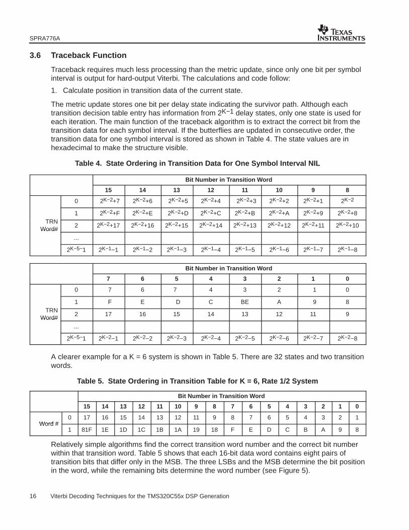
The metric update stores one bit per delay state indicating the survivor path. Although eachtransition decision table entry has information from 2K−1 delay states, only one state is used foreach iteration. The main function of the traceback algorithm is to extract the correct bit from thetransition data for each symbol interval. If the butterflies are updated in consecutive order, thetransition data for one symbol interval is stored as shown in Table 4. The state values are inhexadecimal to make the structure visible.

Table 4. State Ordering in Transition Data for One Symbol Interval NIL

Bit Number in Transition Word

15 14 13 12 11 10 9 8

0 2K−2+7 2K−2+6 2K−2+5 2K−2+4 2K−2+3 2K−2+2 2K−2+1 2K−2

TRN1 2K−2+F 2K−2+E 2K−2+D 2K−2+C 2K−2+B 2K−2+A 2K−2+9 2K−2+8

TRNWord#

2 2K−2+17 2K−2+16 2K−2+15 2K−2+14 2K−2+13 2K−2+12 2K−2+11 2K−2+10Word#

...

2K−5−1 2K−1−1 2K−1−2 2K−1−3 2K−1−4 2K−1−5 2K−1−6 2K−1−7 2K−1−8


7 6 5 4 3 2 1 0

0 7 6 7 4 3 2 1 0

TRN1 F E D C BE A 9 8

TRNWord#

2 17 16 15 14 13 12 11 9Word#

...

2K−5−1 2K−2−1 2K−2−2 2K−2−3 2K−2−4 2K−2−5 2K−2−6 2K−2−7 2K−2−8

A clearer example for a K = 6 system is shown in Table 5. There are 32 states and two transitionwords.

Table 5. State Ordering in Transition Table for K = 6, Rate 1/2 System


15 14 13 12 11 10 9 8 7 6 5 4 3 2 1 0

Word #0 17 16 15 14 13 12 11 9 8 7 6 5 4 3 2 1

Word #1 81F 1E 1D 1C 1B 1A 19 18 F E D C B A 9 8

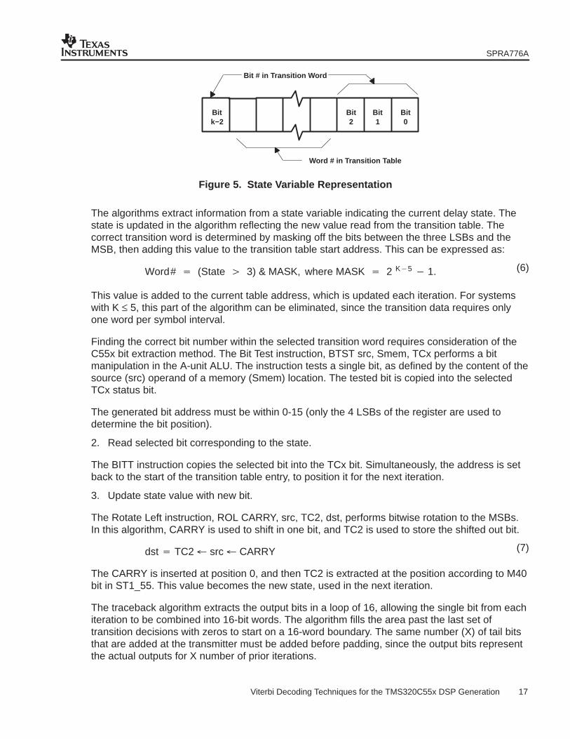
Relatively simple algorithms find the correct transition word number and the correct bit numberwithin that transition word. Table 5 shows that each 16-bit data word contains eight pairs oftransition bits that differ only in the MSB. The three LSBs and the MSB determine the bit positionin the word, while the remaining bits determine the word number (see Figure 5).

SPRA776A


Bit # in Transition Word

Bitk−2

Bit2

Bit1

Bit0

Word # in Transition Table

Figure 5. State Variable Representation

The algorithms extract information from a state variable indicating the current delay state. Thestate is updated in the algorithm reflecting the new value read from the transition table. Thecorrect transition word is determined by masking off the bits between the three LSBs and theMSB, then adding this value to the transition table start address. This can be expressed as:

Word# � (State � 3) & MASK, where MASK � 2 K�5� 1.

This value is added to the current table address, which is updated each iteration. For systemswith K ≤ 5, this part of the algorithm can be eliminated, since the transition data requires onlyone word per symbol interval.

Finding the correct bit number within the selected transition word requires consideration of theC55x bit extraction method. The Bit Test instruction, BTST src, Smem, TCx performs a bitmanipulation in the A-unit ALU. The instruction tests a single bit, as defined by the content of thesource (src) operand of a memory (Smem) location. The tested bit is copied into the selectedTCx status bit.

The generated bit address must be within 0-15 (only the 4 LSBs of the register are used todetermine the bit position).

2. Read selected bit corresponding to the state.

The BITT instruction copies the selected bit into the TCx bit. Simultaneously, the address is setback to the start of the transition table entry, to position it for the next iteration.

3. Update state value with new bit.

The Rotate Left instruction, ROL CARRY, src, TC2, dst, performs bitwise rotation to the MSBs.In this algorithm, CARRY is used to shift in one bit, and TC2 is used to store the shifted out bit.

dst � TC2 � src � CARRY

The CARRY is inserted at position 0, and then TC2 is extracted at the position according to M40bit in ST1_55. This value becomes the new state, used in the next iteration.

The traceback algorithm extracts the output bits in a loop of 16, allowing the single bit from eachiteration to be combined into 16-bit words. The algorithm fills the area past the last set oftransition decisions with zeros to start on a 16-word boundary. The same number (X) of tail bitsthat are added at the transmitter must be added before padding, since the output bits representthe actual outputs for X number of prior iterations.

(6)

(7)

SPRA776A


3.7 Benchmarks

Based on the previous code examples, generic benchmarks can be developed for systems ofrate 1/n (before puncturing) and any constraint length. The benchmarks use the followingsymbols:

• R = original coding rate = 1/n = input bits/transmitted bits

• PR = puncturing rate = p/q = bits retained/total bits

• FS = original frame size (# bits) before coding

• FR = number of data frames per second

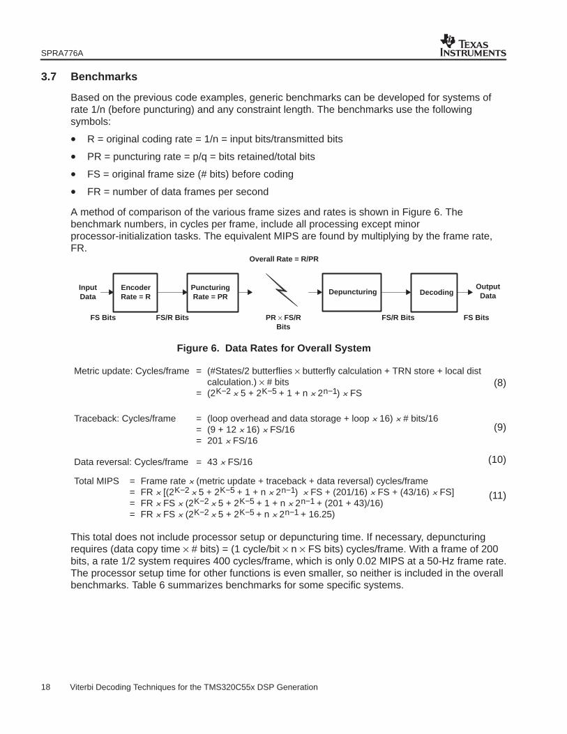
A method of comparison of the various frame sizes and rates is shown in Figure 6. Thebenchmark numbers, in cycles per frame, include all processing except minorprocessor-initialization tasks. The equivalent MIPS are found by multiplying by the frame rate,FR.

Overall Rate = R/PR

PR × FS/RBits

FS/R BitsFS Bits FS/R Bits FS Bits

EncoderRate = R

PuncturingRate = PR

Depuncturing DecodingInputData

OutputData

Figure 6. Data Rates for Overall System

Metric update: Cycles/frame = (#States/2 butterflies × butterfly calculation + TRN store + local distcalculation.) × # bits

= (2K−2 � 5 + 2K−5 + 1 + n � 2n−1) � FS

Traceback: Cycles/frame = (loop overhead and data storage + loop � 16) � # bits/16= (9 + 12 � 16) � FS/16= 201 � FS/16

Data reversal: Cycles/frame = 43 � FS/16

Total MIPS = Frame rate � (metric update + traceback + data reversal) cycles/frame= FR � [(2K−2 � 5 + 2K−5 + 1 + n � 2n−1) � FS + (201/16) � FS + (43/16) � FS]= FR � FS � (2K−2 � 5 + 2K−5 + 1 + n � 2n−1 + (201 + 43)/16)= FR � FS � (2K−2 � 5 + 2K−5 + n � 2n−1 + 16.25)

This total does not include processor setup or depuncturing time. If necessary, depuncturingrequires (data copy time × # bits) = (1 cycle/bit × n × FS bits) cycles/frame. With a frame of 200bits, a rate 1/2 system requires 400 cycles/frame, which is only 0.02 MIPS at a 50-Hz frame rate.The processor setup time for other functions is even smaller, so neither is included in the overallbenchmarks. Table 6 summarizes benchmarks for some specific systems.

(8)

(9)

(10)

(11)

SPRA776A


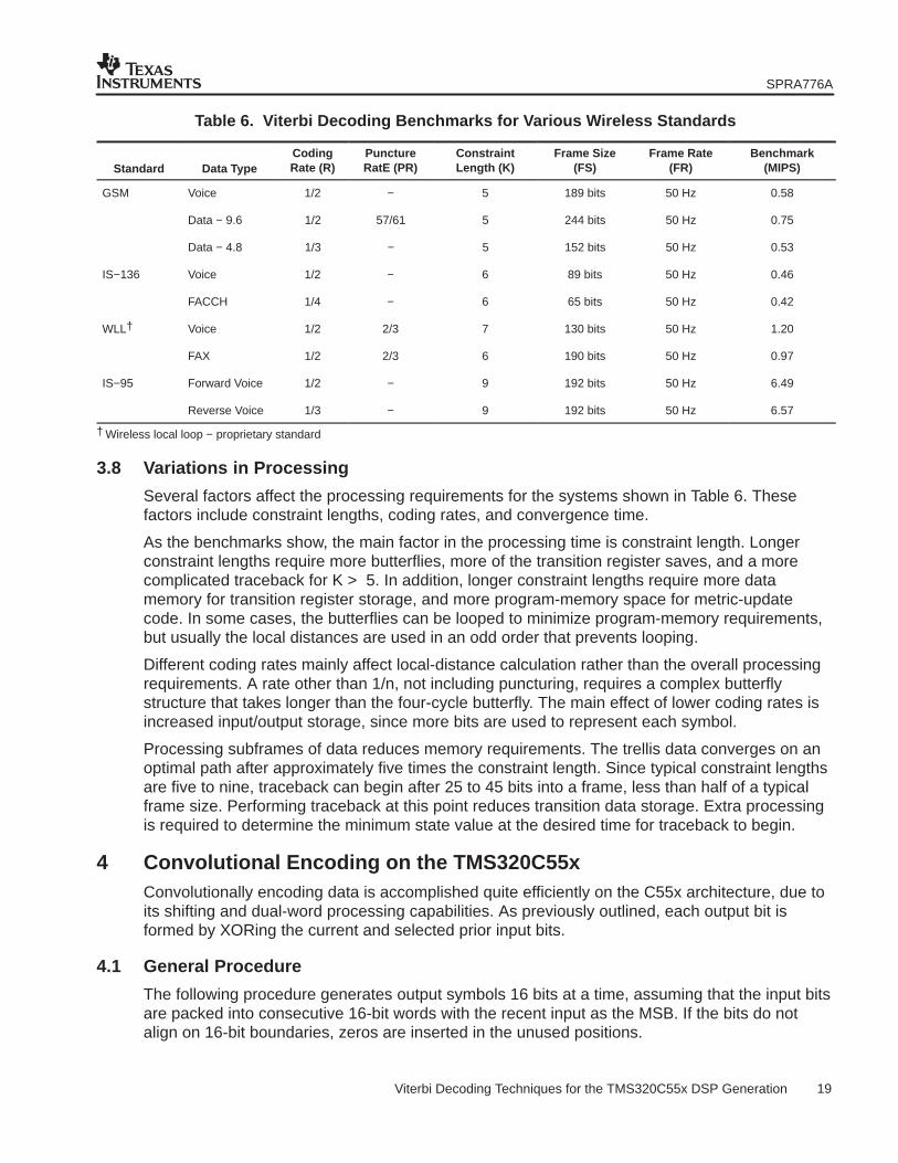
Table 6. Viterbi Decoding Benchmarks for Various Wireless Standards

Standard Data TypeCodingRate (R)

PunctureRatE (PR)

ConstraintLength (K)

Frame Size(FS)

Frame Rate(FR)

Benchmark(MIPS)

GSM Voice 1/2 − 5 189 bits 50 Hz 0.58

Data − 9.6 1/2 57/61 5 244 bits 50 Hz 0.75

Data − 4.8 1/3 − 5 152 bits 50 Hz 0.53

IS−136 Voice 1/2 − 6 89 bits 50 Hz 0.46

FACCH 1/4 − 6 65 bits 50 Hz 0.42

WLL† Voice 1/2 2/3 7 130 bits 50 Hz 1.20

FAX 1/2 2/3 6 190 bits 50 Hz 0.97

IS−95 Forward Voice 1/2 − 9 192 bits 50 Hz 6.49

Reverse Voice 1/3 − 9 192 bits 50 Hz 6.57

† Wireless local loop − proprietary standard

3.8 Variations in Processing

Several factors affect the processing requirements for the systems shown in Table 6. Thesefactors include constraint lengths, coding rates, and convergence time.

As the benchmarks show, the main factor in the processing time is constraint length. Longerconstraint lengths require more butterflies, more of the transition register saves, and a morecomplicated traceback for K > 5. In addition, longer constraint lengths require more datamemory for transition register storage, and more program-memory space for metric-updatecode. In some cases, the butterflies can be looped to minimize program-memory requirements,but usually the local distances are used in an odd order that prevents looping.

Different coding rates mainly affect local-distance calculation rather than the overall processingrequirements. A rate other than 1/n, not including puncturing, requires a complex butterflystructure that takes longer than the four-cycle butterfly. The main effect of lower coding rates isincreased input/output storage, since more bits are used to represent each symbol.

Processing subframes of data reduces memory requirements. The trellis data converges on anoptimal path after approximately five times the constraint length. Since typical constraint lengthsare five to nine, traceback can begin after 25 to 45 bits into a frame, less than half of a typicalframe size. Performing traceback at this point reduces transition data storage. Extra processingis required to determine the minimum state value at the desired time for traceback to begin.

4 Convolutional Encoding on the TMS320C55xConvolutionally encoding data is accomplished quite efficiently on the C55x architecture, due toits shifting and dual-word processing capabilities. As previously outlined, each output bit isformed by XORing the current and selected prior input bits.

4.1 General Procedure

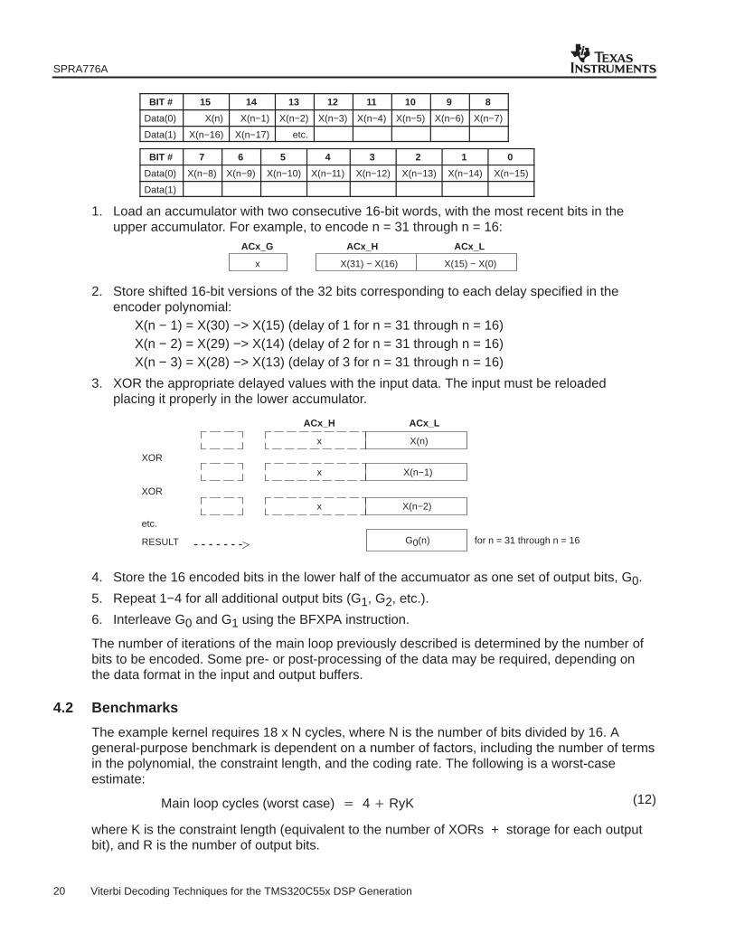
The following procedure generates output symbols 16 bits at a time, assuming that the input bitsare packed into consecutive 16-bit words with the recent input as the MSB. If the bits do notalign on 16-bit boundaries, zeros are inserted in the unused positions.

SPRA776A


BIT # 15 14 13 12 11 10 9 8

Data(0) X(n) X(n−1) X(n−2) X(n−3) X(n−4) X(n−5) X(n−6) X(n−7)

Data(1) X(n−16) X(n−17) etc.

BIT # 7 6 5 4 3 2 1 0

Data(0) X(n−8) X(n−9) X(n−10) X(n−11) X(n−12) X(n−13) X(n−14) X(n−15)

Data(1)

1. Load an accumulator with two consecutive 16-bit words, with the most recent bits in theupper accumulator. For example, to encode n = 31 through n = 16:

x

ACx_G ACx_H ACx_L

X(15) − X(0)X(31) − X(16)

2. Store shifted 16-bit versions of the 32 bits corresponding to each delay specified in theencoder polynomial:

X(n − 1) = X(30) −> X(15) (delay of 1 for n = 31 through n = 16)X(n − 2) = X(29) −> X(14) (delay of 2 for n = 31 through n = 16)X(n − 3) = X(28) −> X(13) (delay of 3 for n = 31 through n = 16)

3. XOR the appropriate delayed values with the input data. The input must be reloadedplacing it properly in the lower accumulator.

ACx_H ACx_L

X(n)

X(n−1)

X(n−2)x

x

x

XOR

XOR

G0(n)

etc.

RESULT for n = 31 through n = 16

4. Store the 16 encoded bits in the lower half of the accumuator as one set of output bits, G0.

5. Repeat 1−4 for all additional output bits (G1, G2, etc.).

6. Interleave G0 and G1 using the BFXPA instruction.

The number of iterations of the main loop previously described is determined by the number ofbits to be encoded. Some pre- or post-processing of the data may be required, depending onthe data format in the input and output buffers.

4.2 Benchmarks

The example kernel requires 18 x N cycles, where N is the number of bits divided by 16. Ageneral-purpose benchmark is dependent on a number of factors, including the number of termsin the polynomial, the constraint length, and the coding rate. The following is a worst-caseestimate:

Main loop cycles (worst case) � 4 � RyK

where K is the constraint length (equivalent to the number of XORs + storage for each outputbit), and R is the number of output bits.

(12)

SPRA776A


5 Conclusion

Convolutional coding is used by communication systems to improve performance in thepresence of noise. The Viterbi Algorithm and its variations are the preferred methods forextracting data from the encoded streams, since it minimizes the number of operations for eachsymbol received. The TMS320C55x generation of DSPs allows high Viterbi decodingperformance. The core Viterbi butterfly can be calculated at a rate approaching three cycles perbutterfly through the use of a splittable ALUs and a dual accumulator.

From the benchmarking equations outlined in this application report, users can quicklydetermine the processing requirements for any rate 1/n Viterbi decoder.

6 References1. Ziemer, R.E., and Peterson, R. L,, Introduction to Digital Communication, Chapter 6:

“Fundamentals of Convolutional Coding,” New York: Macmillan Publishing Company.

2. Edwards, Gwyn, “Forward Error Correction Encoding and Decoding,” Stanford TelecomApplication Note 108, 1990.

3. TMS320C55x User’s Guide, Digital Signal Processing Products, Texas Instruments, 1995.

4. Clark, G.C. Jr. and Cain, J.B. Error-Correction Coding for Digital Communications, NewYork: Plenum Press.

5. Michelson, A.M., and Levesque, A.H., Error-Control Techniques for DigitalCommunications, John Wiley & Sons, 1985.

6. Chishtie, Mansoor, “A TMS320C53-Based Enhanced Forward Error-Correction Schemefor U.S. Digital Cellular Radio,” Telecommunications Applications With the TMS320C5xDSPs, 1994, pp. 103-109.

7. “Using Punctured Code Techniques with the Q1401 Viterbi Decoder,” QualcommApplication Note AN1401-2a.

8. Viterbi Decoding Techniques in the TMS320C54x Generation (SPRA071).

7 Bibliography

Chishtie, Mansoor, “U.S. Digital Cellular Error-Correction Coding Algorithm Implementation onthe TMS320C5x,” Telecommunications Applications With the TMS320C5x DSPs, 1994, pp.63-75.

Chishtie, Mansoor, “Viterbi Implementation on the TMS320C5x for V.32 Modems,”Telecommunications Applications With the TMS320C5x DSPs, 1994, pp. 77-101.

SPRA776A


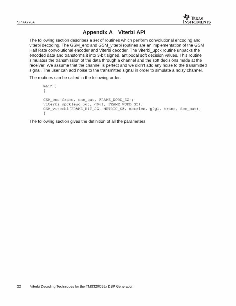
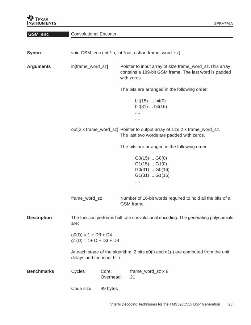
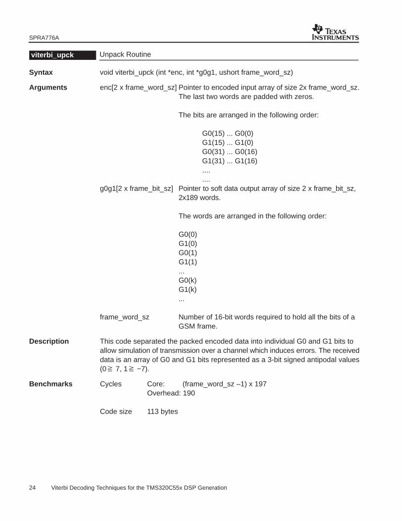
Appendix A Viterbi APIThe following section describes a set of routines which perform convolutional encoding andviterbi decoding. The GSM_enc and GSM_viterbi routines are an implementation of the GSMHalf Rate convolutional encoder and Viterbi decoder. The Viterbi_upck routine unpacks theencoded data and transforms it into 3-bit signed, antipodal soft decision values. This routinesimulates the transmission of the data through a channel and the soft decisions made at thereceiver. We assume that the channel is perfect and we didn’t add any noise to the transmittedsignal. The user can add noise to the transmitted signal in order to simulate a noisy channel.

The routines can be called in the following order:

main(){

GSM_enc(frame, enc_out, FRAME_WORD_SZ);viterbi_upck(enc_out, g0g1, FRAME_WORD_SZ);GSM_viterbi(FRAME_BIT_SZ, METRIC_SZ, metrics, g0g1, trans, dec_out);}

The following section gives the definition of all the parameters.

SPRA776A


Convolutional EncoderGSM_enc

Syntax void GSM_enc (int *in, int *out, ushort frame_word_sz)

Arguments in[frame_word_sz] Pointer to input array of size frame_word_sz.This array contains a 189-bit GSM frame. The last word is padded with zeros.

The bits are arranged in the following order:

bit(15) .... bit(0)bit(31) ... bit(16)........

out[2 x frame_word_sz] Pointer to output array of size 2 x frame_word_sz.The last two words are padded with zeros.


G0(15) ... G0(0)G1(15) ... G1(0)G0(31) ... G0(16)G1(31) ... G1(16)........

frame_word_sz Number of 16-bit words required to hold all the bits of a GSM frame.

Description The function performs half rate convolutional encoding. The generating polynomialsare:

g0(D) = 1 + D3 + D4g1(D) = 1+ D + D3 + D4

At each stage of the algorithm, 2 bits g0(i) and g1(i) are computed from the unit delays and the input bit i.

Benchmarks Cycles Core: frame_word_sz x 8Overhead: 21

Code size 49 bytes

SPRA776A


Unpack Routineviterbi_upck

Syntax void viterbi_upck (int *enc, int *g0g1, ushort frame_word_sz)

Arguments enc[2 x frame_word_sz] Pointer to encoded input array of size 2x frame_word_sz.The last two words are padded with zeros.


G0(15) ... G0(0)G1(15) ... G1(0)G0(31) ... G0(16)G1(31) ... G1(16)........

g0g1[2 x frame_bit_sz] Pointer to soft data output array of size 2 x frame_bit_sz, 2x189 words.

The words are arranged in the following order:

G0(0)G1(0)G0(1)G1(1)...G0(k)G1(k)...

frame_word_sz Number of 16-bit words required to hold all the bits of a GSM frame.

Description This code separated the packed encoded data into individual G0 and G1 bits to allow simulation of transmission over a channel which induces errors. The receiveddata is an array of G0 and G1 bits represented as a 3-bit signed antipodal values(0� 7, 1� −7).

Benchmarks Cycles Core: (frame_word_sz –1) x 197Overhead: 190

Code size 113 bytes

SPRA776A


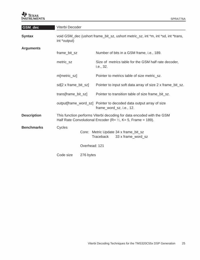
Viterbi DecoderGSM_dec

Syntax void GSM_dec (ushort frame_bit_sz, ushort metric_sz, int *m, int *sd, int *trans, int *output)

Argumentsframe_bit_sz Number of bits in a GSM frame, i.e., 189.

metric_sz Size of metrics table for the GSM half rate decoder, i.e., 32.

m[metric_sz] Pointer to metrics table of size metric_sz.

sd[2 x frame_bit_sz] Pointer to input soft data array of size 2 x frame_bit_sz.

trans[frame_bit_sz] Pointer to transition table of size frame_bit_sz.

output[frame_word_sz] Pointer to decoded data output array of size frame_word_sz, i.e., 12.

Description This function performs Viterbi decoding for data encoded with the GSMHalf Rate Convolutional Encoder (R= �, K= 5, Frame = 189).

Benchmarks CyclesCore: Metric Update 34 x frame_bit_sz

Traceback 33 x frame_word_sz

Overhead: 121

Code size 276 bytes

SPRA776A

26 Viterbi Decoding Techniques for TMS320C54x DSP Generation

Appendix B GlossaryAntipodal value

A diametrically opposite value; for instance 1 for −1, 0 for +1, x(t) and x(t)

Block codeA fixed-length code format that consists of message and parity bits (block = m + p)

ButterflyThe butterfly flowgraph diagram represents the smallest computational unit in a logic calculationshowing the encoding or decoding of outputs from given inputs.

Constellation pointsPoints corresponding to specific magnitude and phase values produced by an encoder.Constellation diagrams show the real and imaginary axis or vector spaces in two dimensions.

Constraint lengthThe range of blocks over which recurrent or convolutional-coded check bits are operative. Theoutput bits are dependent on the message bits in the previous m−1 bits (where m is theconstraint length).

Euclidean distanceEuclidean distance refers to the distance between two M-dimensional vectors, as opposed to theHamming distance that refers to the number of bits that are different. It is analogous to theanalog distance as opposed to the digital distance.

Hamming distanceNamed after R. L. Hamming, the Hamming distance of a code is the number of bit positions inwhich one valid code word differs from another valid code word.

Local distanceThe distance in a path state calculated to a symbol or constellation point from the current input

MetricA function in mathematics relating to the separation of two points relating to the Hamming orEuclidean distance between two code words.

Puncture codingA technique that selectively and periodically removes bits from an encoder output to effectivelyraise the data rate. The output from a convolutional encoder passes through a gate circuitcontrolled by a puncture matrix that defines the characteristics of the error protection for the bitsin a block of information.

Survivor pathIn a Viterbi decoder, the survivor path is the minimum accumulated distance (shortest time)calculated for each input path.

TrellisA tree diagram where the branches following certain nodes are identical. These nodes (orstates), when merged with similar states, form a graph that does not grow beyond 2k−1 where kis the constraint length.

Viterbi decodingA maximum likelihood decoding algorithm devised by A. J. Viterbi in 1967. The decoder uses asearch tree or trellis structure and continually calculates the Hamming (or Euclidean) distancebetween received and valid code words within the constraint length.

IMPORTANT NOTICETexas Instruments Incorporated and its subsidiaries (TI) reserve the right to make corrections, modifications, enhancements, improvements,and other changes to its products and services at any time and to discontinue any product or service without notice. Customers shouldobtain the latest relevant information before placing orders and should verify that such information is current and complete. All products aresold subject to TI’s terms and conditions of sale supplied at the time of order acknowledgment.TI warrants performance of its hardware products to the specifications applicable at the time of sale in accordance with TI’s standardwarranty. Testing and other quality control techniques are used to the extent TI deems necessary to support this warranty. Except wheremandated by government requirements, testing of all parameters of each product is not necessarily performed.TI assumes no liability for applications assistance or customer product design. Customers are responsible for their products andapplications using TI components. To minimize the risks associated with customer products and applications, customers should provideadequate design and operating safeguards.TI does not warrant or represent that any license, either express or implied, is granted under any TI patent right, copyright, mask work right,or other TI intellectual property right relating to any combination, machine, or process in which TI products or services are used. Informationpublished by TI regarding third-party products or services does not constitute a license from TI to use such products or services or awarranty or endorsement thereof. Use of such information may require a license from a third party under the patents or other intellectualproperty of the third party, or a license from TI under the patents or other intellectual property of TI.Reproduction of TI information in TI data books or data sheets is permissible only if reproduction is without alteration and is accompaniedby all associated warranties, conditions, limitations, and notices. Reproduction of this information with alteration is an unfair and deceptivebusiness practice. TI is not responsible or liable for such altered documentation. Information of third parties may be subject to additionalrestrictions.Resale of TI products or services with statements different from or beyond the parameters stated by TI for that product or service voids allexpress and any implied warranties for the associated TI product or service and is an unfair and deceptive business practice. TI is notresponsible or liable for any such statements.TI products are not authorized for use in safety-critical applications (such as life support) where a failure of the TI product would reasonablybe expected to cause severe personal injury or death, unless officers of the parties have executed an agreement specifically governingsuch use. Buyers represent that they have all necessary expertise in the safety and regulatory ramifications of their applications, andacknowledge and agree that they are solely responsible for all legal, regulatory and safety-related requirements concerning their productsand any use of TI products in such safety-critical applications, notwithstanding any applications-related information or support that may beprovided by TI. Further, Buyers must fully indemnify TI and its representatives against any damages arising out of the use of TI products insuch safety-critical applications.TI products are neither designed nor intended for use in military/aerospace applications or environments unless the TI products arespecifically designated by TI as military-grade or "enhanced plastic." Only products designated by TI as military-grade meet militaryspecifications. Buyers acknowledge and agree that any such use of TI products which TI has not designated as military-grade is solely atthe Buyer's risk, and that they are solely responsible for compliance with all legal and regulatory requirements in connection with such use.TI products are neither designed nor intended for use in automotive applications or environments unless the specific TI products aredesignated by TI as compliant with ISO/TS 16949 requirements. Buyers acknowledge and agree that, if they use any non-designatedproducts in automotive applications, TI will not be responsible for any failure to meet such requirements.Following are URLs where you can obtain information on other Texas Instruments products and application solutions:Products ApplicationsAmplifiers amplifier.ti.com Audio www.ti.com/audioData Converters dataconverter.ti.com Automotive www.ti.com/automotiveDLP® Products www.dlp.com Broadband www.ti.com/broadbandDSP dsp.ti.com Digital Control www.ti.com/digitalcontrolClocks and Timers www.ti.com/clocks Medical www.ti.com/medicalInterface interface.ti.com Military www.ti.com/militaryLogic logic.ti.com Optical Networking www.ti.com/opticalnetworkPower Mgmt power.ti.com Security www.ti.com/securityMicrocontrollers microcontroller.ti.com Telephony www.ti.com/telephonyRFID www.ti-rfid.com Video & Imaging www.ti.com/videoRF/IF and ZigBee® Solutions www.ti.com/lprf Wireless www.ti.com/wireless

Mailing Address: Texas Instruments, Post Office Box 655303, Dallas, Texas 75265Copyright © 2009, Texas Instruments Incorporated

http://amplifier.ti.com

http://www.ti.com/audio

http://dataconverter.ti.com

http://www.ti.com/automotive

http://www.dlp.com

http://www.ti.com/broadband

http://dsp.ti.com

http://www.ti.com/digitalcontrol

http://www.ti.com/clocks

http://www.ti.com/medical

http://interface.ti.com

http://www.ti.com/military

http://logic.ti.com

http://www.ti.com/opticalnetwork

http://power.ti.com

http://www.ti.com/security

http://microcontroller.ti.com

http://www.ti.com/telephony

http://www.ti-rfid.com

http://www.ti.com/video

http://www.ti.com/lprf

http://www.ti.com/wireless

Date post:	06-Mar-2018
Category:	Documents
Upload:	truongtuong
View:	250 times
Download:	2 times

Viterbi Decoding Techniques for the TMS320C55x DSP ... · PDF fileSPRA776A Viterbi Decoding...

Documents