VLF PHASE TRACKING FOR PTTI APPLICATION

by

Dr. F. H. Reder

Dr. Reder is Chief, Antennas and Geophysical Effects Research TechnicalArea, Electronics Technology and Devices Laboratory, U.S. Army ElectronicsCommand, Fort Monmouth, New Jersey.

1.0 PURPOSE OF PAPER

The purpose of this tutorial paper is to give a short review of some

basic facts about VLF propagation for PTTI applications, and to discuss equip-

ment problems and the effects of ionospheric disturbances.

2.0 SOME BASIC FACTS ABOUT VLF PROPAGATION

For the theory of VLF propagation one may consult the books of Budden1

2and Wait . Practical aspects may be found in the VLF Radio Engineering book

3by Watt

VLF waves propagate in the wave guide provided by the ground and by

the ionospheric shell. When close to a transmitter it is convenient to de-

scribe observed phenomena by means of ray theory. Beyond the distance of

1, 000 kilometers or so, it is advantageous to use mode theory with a mode

being one of the solutions of Maxwell's equations for a bounded propagation

medium.

Normally, we have to worry only about the first- and second-order

modes. These modes differ by three important parameters: (1) their phase

velocities (the higher the mode number, the higher the phase velocity);

-117-

(2) their attentuation rates (below 25 kilohertz, the higher order modes norm-ally have higher attenuation per megameter); (3) their excitation functions(at a given time of the day one mode is better excited by a transmitter than

the other). For many applications, one can use the simple flat-earth model

with infinite conductivity on the ground and in the ionosphere. If greaterprecision is desired, a spherical model should be used, with appropriate

approximations for the ionospheric conductivity as a function of height andwith inclusion of the geomagnetic field. A very useful approximation for the

ionospheric conductivity is given by an exponential function depending on

some reference height and a gradient. Pertinent tables have been published

by Wait and Spies for determining phase velocity, excitation function in db

and loss in db/Mm as functions of reference height and gradient. Normallyone assumes for daytime propagation a reference height of 70 Km and a gradient

of 0.3 Km , and for nighttime a reference height of 90 Km and a gradient of

0. 5 Km

For many applications of VLF there are some simple rules of thumb by

which one can interpret observed phase and amplitude anomalies.

One rule is that any natural disturbance (except a solar eclipse) lowersthe reference height. That means the phase velocity will go up for both thefirst- and the second-order modes whereas the amplitude for the first-ordermode may go up or down depending upon frequency and the amplitude of the

second-order mode always goes down. When the gradient increases, whichseems to be the usual case in a disturbance, the phase velocity decreasesfor all modes, and the amplitude increases (the latter is understandable be-cause with a larger gradient the ionosphere is denser and, therefore, has lessleakage). From this it can be seen that if a disturbance occurs, there are twophase effects which oppose each other: the height reduction will increasethe phase velocity, and the increase of the gradient will decrease the phasevelocity. However, the decrease is negligible when compared to the opposingincrease so, as a general rule, whenever the ionosphere comes down thephase velocity will increase. Amplitude anomalies, on the other hand,

-118-

are not so easily predictable. Below about 18 kilohertz, e.g., solar X-ray

bursts may either cause signal enhancement, no discernible change or signal

loss, depending on signal frequency, path direction and location, and flare

spectrum. Above 20 kilohertz it is quite safe to predict signal enhancementfor solar X-ray flares, regardless of path geometry.

In the event that there is more than one mode present, it is possible tohandle the explanation of many phenomena with a simple vector model.5 The

two mode phasors are computed for the given path, e.g., by using the tables

of Wait and Spies. Then the phasor of the second-order mode is added to

the phasor of the first-order mode. If there is an ionospheric disturbance,

the phasor of the first mode will advance in phase by a certain amount, andthe phasor of the second mode will advance by a larger amount. Depending

on the original positions of the two phasors with respect to each other, anionospheric disturbance can cause a large variety of VLF anomalies. Therecan be an amplitude increase or decrease with practically no phase change,or a phase delay or advance with almost no amplitude change, or any combi-nation of the two.

Another important point is that when a path crosses either a very hugemass of ice or a permafrost area where the electric ground conductivity is

5 ,6low, propagation losses are substantially increased. Therefore, oneshould avoid a path which crosses Greenland or the Antarctic ice.

If one is located as close as 1,000 kilometers or less to a transmitter,one may actually have more trouble in data interpretation than if one is fartheraway, because the EM field will then consist of a ground wave, an ordinaryskywave, and an extraordinary skywave, which is just too much for the ordi-nary operator to handle. So if it is necessary to pick a VLF signal for PTTIapplications, it often is better to select a transmitter which is more than1,000 kilometers away.

-1 19-

3. 0 RECEPTION EQUIPMENT

Figure 1 shows a typical VLF setup. It includes a voltage regulator, 3an emergency power supply (batteries), a frequency standard (Rubidium stan-

dard in this case), two receivers, and a multichannel recorder. The antennas

(loop, whip or long-wire) are not shown. There are many potential trouble

areas, and most of all there are lots of tempting control knobs. It is a very 3good idea to follow the principle: keep your hands off, once everything works

properly. For example, at Fort Monmouth we have a cesium beam frequency 3standard which we have not touched since March, 1967, except for retuning

the Xtal about every three months. This is probably one important reason why Iit is still working so well after almost five years of operation.

A problem with loop antennas is that of waterproofing. A loop is sup- 3posed to be electrostatically shielded by an aluminum tube around it. This

tube has to have one gap otherwise the VLF field could not be picked up. At |

the same time, the tube must be rain-tight, which is accomplished by a non-

metallic fitting over the gap. Although the manufacturer claims that the loops Iare rain-tight, in practice they are not. Exposure to sun, cold, rain, snow

and ice, makes the joints between aluminum tube and non-metallic gap mate- Irial and the seal of the tuning box leaky. As a consequence, the tuning box

will fill up with water and the signal output will decrease. The solution is to Icover all joints with a plastic cover which should be open at the bottom to

let condensed water get out. |

Whips must be protected from dirt splashings on the base insulator.

Also, a good counterpoise (6 radial copper braids) should be maintained to

avoid signal variations due to change of ground moisture.

Cables should not be left lying on the floor where people may step on Ithem and either damage connectors or break their outer shields. Cable con-

nectors are, of course, a major trouble source. Their contacts may corrode,

their pins may get loose, etc.

-120-

.1 &S

1; ... -, -

Ix II.E.

p "0

4

:,=.B ~~ .. '

ri ~~~

.wj,.~ i ~ Bl* w -xs .4e t *

I

I.3' viv$�

�

¾*- I'�AA�. ,�

� C,.'.'A

4i

Figure 1. TYPICAL VLF RECEIVER SETUP

- 1 2 1-

I .

e,,1

OFvW

:j

.7l:1 -

I .

One of the most frequent failure sources in a receiver with a modular

construction are the plugs between modules and chassis. Therefore, when

the receiver fails, the first thing to do is to pull out one by one all the

modules and push them right back. In about 80 percent of the cases, this

may correct the problem.

The recorder shown in Figure 1 has excellent reliability and precision,

but its 10-millivolt full-scale-sensitivity requires great care to avoid ground

loops. It is our experience that such ground loops are particularly difficult

to avoid if the receivers are connected to standby battery supplies (which is

a must to avoid phase jumps during power failures). One indication of such

a problem is nonlinearity of the recorder scale. Another indication is that the

scale does not go to zero because of the presence of a stray voltage. To

avoid this trouble, it is advisable to fasten all equipment needed for the re-

cording tightly into one metal rack. Sometimes it helps to connect appro-

priate ground terminals of the DC supplies, receivers and the frequency stan-

dard by a reasonably heavy copper braid (but too many ground connections may

be self-defeating).

A last remark on reception equipment: always use an RF filter in the

front-end of the receiver, because the signal you tracketh may not be what

thou thinketh. (Can be mirror signal of something else.)

4.0 TRANSMITTER PROBLEMS

Figure 2 shows an example of transmitter phase jumps which we have

had in the past (NAA, NPG, NPM and GBR trackings). The distinct jumps

occurred when the transmitters switched between FSK and CW, because one

mode of operation required an extra filter. The example marked NPM-Fairbanks

is taken from a 1964 recording of NPM at Fairbanks. We were, at first, ex-

tremely happy because it happened to be that the period of this oscillation

was about four minutes, and this period was thought to be a typical period

for electron precipitation. Fortunately, we took a look at records of NPM

- 1 2 2-

C:

,, . I I, beNPG-TANANARIVE I A | -t

O~~~~~~~~~~~~~ I

JULY 20, 1967 I _ _I

A~~I

S 18db50 2 2 20

50 050-NBA-TOKYO 2

JULY 7, 1967 A..... - --. ~r.

0 5

20 21 22 23 U T

Figure 3. EXAMPLES OF VLF SIGNAL INTERFERENCE

- 125-

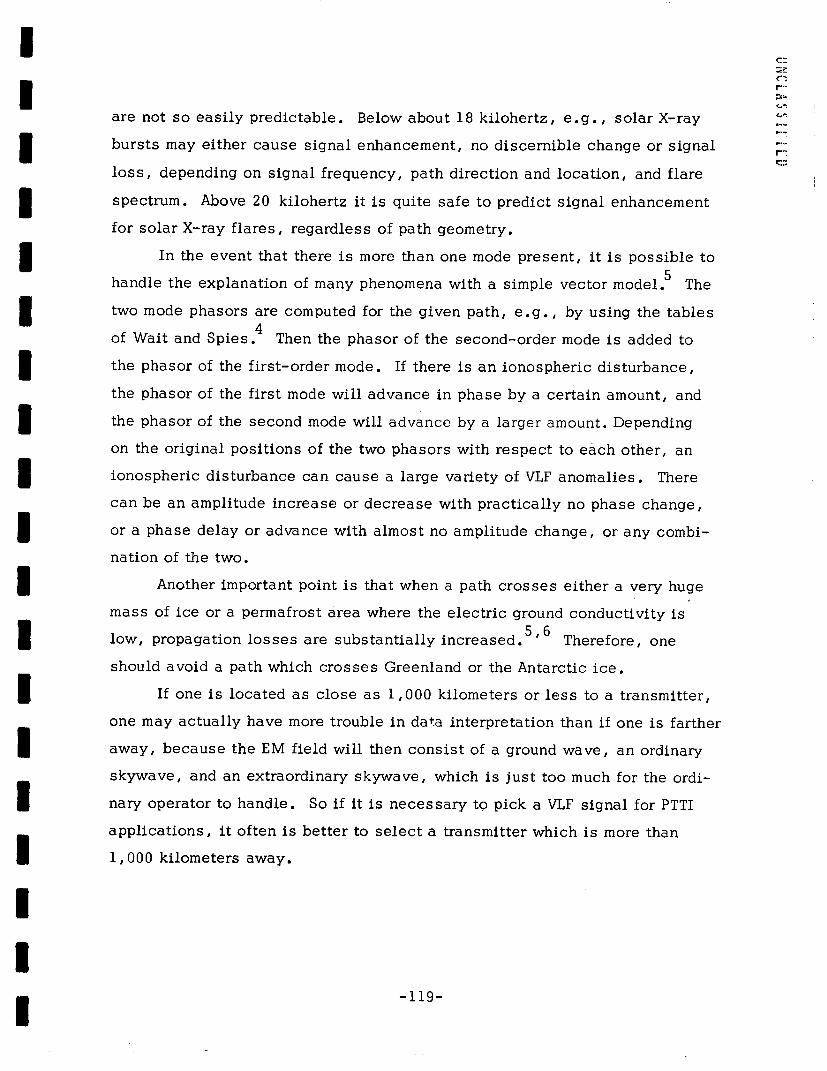
Figure 4 illustrates some typical diurnal phase patterns. More or less

sharply defined phase changes occur during sunset and sunrise at the path

terminals. The dashed curves pertain to the standard deviations with respect

to 14-day averages. The plot, NPM to Deal (summer) shows during the morn-

ing hours (0800-1600) mode interference effects typical for VLF frequencies

above 18-20 kilohertz. The second-order mode which is excited near the

transmitter gets converted at the solar terminator into a first-order mode which

interferes with the first-order mode passing through the terminator. As the

terminator moves, the two first-order mode phasors observed at the receiver

site rotate with respect to each other, causing a series of amplitude minima

and phase steps.

In order to understand these diurnal phase patterns, it helps very much

to have available sunlight-twilight-night charts ' plotted for two week

ILS

50

ae

Ps

GBR - BEIRUT (FALL)

- jW0

.,

-1I2 18 24 06 I,

_T_ I ~~~~~~~~~~~~~~~~I

NSS-BEIRUT (SUMMER)

t-t't' -' .~2 18 24 06 UT 12

Figure 4. SOME TYPICAL DIURNAL PHASE PATTERNS ANDSTANDARD DEVIATIONS

-126-

IIII3

IIIII

50

i

II

l

intervals with a map overlay (Figure 5). To find out at what times the sun

will rise on a particular path, one plots the path on the map overlay -- for

intance, NPM to Sao Paulo -- picks the terminator chart for the right date, lays

the map over the chart and turns it until one of the path terminals passes

through the terminator. Then the time the sun will rise or set will be indi-

cated by the angular position of the map overlay with respect to the termina-tor chart (time scale along circumference of chart is not shown in Figure 5).

Figure 5. EXAMPLE OF A VLF PATH LOCATION WITH RESPECT TOSOLAR TERMINATOR (S Stands for Stockholm)

Figure 6 proves that these mode interference effects can also be pres-

ent in the evening.

A very undesirable consequence of mode interference is shown in the

lower part of Figure 7. In the evening the pattern develops apparently in a

normal way (indicating a phase delay). At nighttime the phase becomes

usually a little more disturbed. Then in the morning, instead of returning

- 1 2 7-

A

DB

40

20

I I I I I I I I I I

15 19 23 22 02 UT 06

Figure 6. MODE INTERFERENCE DURING EVENING SHIFT

Figure 7.

Is 24 06 12 UT

EXAMPLE FOR PARTICULAR MODE INTERFERENCE OBSERVEDON NSS-C (Rivadavia)

- 12 8-

p s

100

II'I

IIIIIIiI

IIIIII

C:1

to the level of the previous day as one would expect, the phase undergoes -an additional cycle advance before settling down for the daytime. Such a

cycle advance due to mode interference is not much of a problem if one has

a good reference standard, but otherwise it can be a lot of trouble. The onlyconsolation is that it is known that the correction has to be exactly one

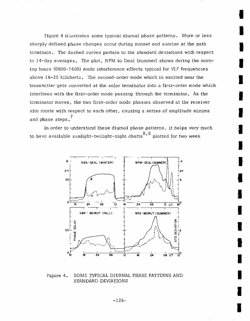
cycle.Figure 8 depicts a case of mode interference observed on NAA-Deal

(Fort Monmouth), a path of medium length (1,000 kilometers). Depending on

the ionospheric activity and depending on the season, almost any pattern can

be observed: phase advance in morning and delay in evening (#4, normal),

advance in morning and evening (#13), delay in morning and evening (#5),

and delay in morning, advance in evening (#10, reversed pattern).

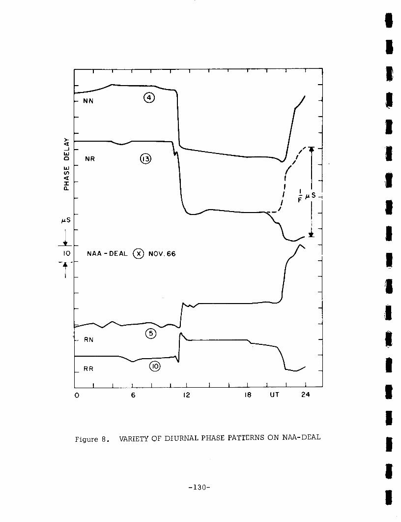
Another undesirable feature occurs on some transmissions crossing the

magnetic equator. For instance, Figure 9 shows the diurnal phase pattern ofHaiku (12.2 kilohertz) to Brisbane, Australia in comparison with the normaldiurnal patterns observed at Tokyo and Deal.5 The diurnal shift observed at

Brisbane is much smaller than expected. Of course, one thinks immediatelycycle slips occurred at about 0700 and 1800 and ought to be corrected . But

if one corrects the night portion by 1 cycle the diurnal pattern will be toohigh. So one has a choice of whether one wants the pattern to be too low or

too high.

Figure 10 gives an example of a path which is just so long that the

first-order and the second-order modes are almost equal in amplitude andnearly out of phase with each other during the night. One observes then twophasors at the receiver site which almost cancel each other. Then the slight-est ionospheric disturbance can cause relatively big phase changes. As aresult, nighttime phase may either show a "cave-in" or a "blow-out" (notshown in figure), with the phase difference being again exactly 1 cycle.

- 129-

0 6 12 18 UT 24

Figure 8. VARIETY OF DIURNAL PHASE PATTERNS ON NAA-DEAL

-130-

24

Figure 9.

Figure 10.

18 12 6 4-UT

PECULIAR DIURNAL PHASE PATTERN OF NPM-BRISBANE ASCOMPARED WITH THOSE OF NPM-TOKYO AND NPM-DEAL

EXAMPLES FOR MODE INTERFERENCE DURING NIGHTTIME ONPATHS FOR WHICH FIRST- AND SECOND-ORDER MODES AREALMOST EQUAL IN STRENGTH AND OUT OF PHASE WITHEACH OTHER

-13 1-

C.

r -

Or

rrC:_

0

An example of the so-called "morning layer" ° is shown in Figure 11.

If one has a signal path which passes through the morning terminator almost

simultaneously along its entire length, one observes a temporary additional

phase advance which will typically last for about 90 minutes, before the

phase will reach its regular daylight value. The advance, for instance, of

GBR to Cordoba, Argentina, is of the order of 10 microseconds. On the path

from NBA to Fort Monmouth, it is of the order of a maximum of 5 microseconds.

The anomaly is caused by a temporary excess of electrons in the lower iono-

sphere and will be the larger the longer the path is and the faster the entire

path crosses the terminator.

SUNRISE AT

4 90KM 03 50 KMDhJ 70 KM0w

90 KM

70 KM NA ACORDOBA

50 \ 16 M AR 67_

\ _ ~~~~~~~GBR -S. PAULO50

0 I I _ -I\ i' _

7 9 11 13 UT 15

Figure 11. EFFECT OF SUNRISE LAYER ON VLF PHASE

Figure 12 gives an example of antipodal interference. The short path

runs across Greenland; the long path runs across the Antarctic ice cap. In

-132-

II

IiIIIIIII

's-

NPG - TANANARIVE

100

a.

50-

0 1

CalS12 18 24 06 UT 12

Figure 12. ANTIPODAL INTERFERENCE ON NPG-TANANARIVE

summer when Greenland is in sunlight, the attenuation over Greenland is ex-tremely strong -- approximately 20 to 30 db. This signal is then cut off andthe signal to Madagascar comes from NLK via the Antarctic which is in night,and therefore, the losses are not so high. In winter it is just the other way

around: Greenland is in night and so it affects the signal only slightly, whilethe Antarctic is in daylight and cuts off the long-path signal. During springand fall both signals are present at Tananarive. Reading from the top ofFigure 12 down, the first curve pertains to September (mixed); the second

curve to January (signal from Greenland only); and the third curve to July when

- 1 3 3 -

the signal comes only via the Antarctic. Consequently, the January and July

patterns are out of phase with each other. We see that the huge ice masses

act as season-triggered filters.

7.0 DISTURBANCES

The upper left part of Figure 13 depicts some typical phase and ampli-

tude anomalies caused by sudden ionospheric disturbances (SID's) due to solar

X-ray flares. 11 As expected for single-mode signals which are free of anti- 5podal interference, the phase always advances. In this example, the ampli-

tudes increased. However, as mentioned before, amplitude will definitely be

enhanced only at frequencies above 18-20 kilohertz. E~g., the signal GBR-

Tananarive usually (but not always) indicates an amplitude decrease during 5an SID.

The upper right-hand part of Figure 13 demonstrates frequency depend-

ence of VLF phase anomalies due to SID's. the lower the frequency, the larger

the anomaly. For instance, on 29 December 1968, Haiku 10.2 to Deal deviated Iby almost 80 microseconds, Haiku 13.6 to Deal by about 50 microseconds,

whereas the NPM 23.4 kilohertz to Deal anomaly was only 20 microseconds. |

All three paths are of equal lengths. The NLK 18.5 kilohertz-Deal anomaly

was smaller again because this path is considerably shorter. 5The lower part of Figure 13 illustrates what can happen to long-path

signals on a day of very high solar activity. SID's followed one another all |

day long and the phase of Aldra 12.3 kilohertz -- Tananarive was advanced

by an average of 20 microseconds during the time 0500Z to 1200Z.

If at all possible, one should never record phase alone, but always

phase and amplitude. How advisable this is for proper interpretation of VLF 3phase anomalies is illustrated by Figure 14. On 2 September 1967, the SID

at about 2040Z is clearly indicated by a phase advance and amplitude in- 5crease with distinct peaks and typical recovery. The phase advance commenc-

ing shortly after 2200 hints at another SID but the lack of any amplitude

-134-

Figure 13. SOLAR X-RAY EFFECTS ON VLF SIGNALS

ps

20

101-

Is

40

30

20

20 21

2 SEP 196722 23 UT

10I

17 19 20 UT

db20

10

iS

14 AUG 1965

Figure 14. EXAMPLES FOR PHASE JUMPS CAUSED BY EQUIPMENT FAILURESBUT LOOKING LIKE SID'S

-135-

NPM- DEAL

AAASID TRANSM.

PHASE JUMP

I I I

-_ , GBR - DEALa IIiIUV

-t GBR- C. RIVDAa.\- -

C=

cl,r-:;I.?� 1.41n

-r

rrtz,..:

anomaly points to a transmitter phase jump. The GBR-C. Rivadavia 3(Argentina) phase anomaly on 14 August also has all the appearance of an

SID, but the GBR-Deal recording clearly indicates a GBR phase jump. The Ionset is too sudden for an SID, there is no phase recovery and the amplitude

shows no enhancement (typical for that path). Why does the GBR-C. Rivadavia l

anomaly look like an SID? Poor signal-to-noise ratio on this long path re-

quired use of an extra-long time-constant (150 sec), which rounded off the

lower portion of the phase recording and the diurnal evening shift commencing

slowly at 1700 and accelerating around 1800 provided a decieving simulation Iof the recovery of an SID. Had a reliable amplitude recording been taken at

C. Rivadavia, it would have been obvious immediately that no SID occurred

between 1700 and 1800 on 14 August 1965.

A short path, like Forestport 13.6 kilohertz-Deal (350 kilometers) can Iresult in reversed SID's. Figure 15 is an example: GBR to Sao Paulo and

Trinidad to Deal are paths longer than 3,000 Km and their SID's are normal I(phase advance), while the SID's observed on Forestport-13.6 kilohertz-Deal

are reversed (phase delay). This behavior can be explained by a phasor model Iusing two modes as discussed before.

-_ sTRVI3i DEFHV L ___ v[Dmtr~

DEALX_ IYYE13 FDEHV -___zv; _ __> =!rzr, fz=

I

Figure 15. REVERSED SID PHASE ANOMALY ON FORESTPORT 13.6 KILOHERTZ-DEAL gI

-136-

Figure 16 shows some examples of electron precipitation effects. The

electrons come directly from the sun or from the radiation belts and have been

detected both at high and middle-latitudes. What is typical about them? Let

us first take the path from NBA to Deal on 28/29 March 1966. At about 1908Z

an SID occurred and it recovered within about 2.5 hours without discernible

after effects. On the other hand, on GBZ and NPG to Deal we see the X-ray

SID effects followed by new anomalies lasting to beyond 0300 on 29 March.

Typically, electron effects last for several hours (two to eight and more).

Another example for electrons is shown for 26/27 December 1966.

NPG ~~~DEAL -1966_

NPG

-jW IX 2,9 MARCH0

-NBA / _____

a-

I0

-GBR

- - - -PREVIOUS QUIET DAY

19 21 23 01 UT 03

Figure 16. EXAMPLES OF ELECTRON PRECIPITATION EFFECTS

- 13 7-

C-C:

rC

r-

rrUs:

For PTTI purposes, one should avoid a polar path, because polar paths

may be affected strongly by protons from the sun and these effects may last

up to 10 days. Events of proton precipitation often lead to blackout of HF

communication through the polar cap. Therefore, a proton precipitation

event is called Polar Cap Absorption (PCA). Figure 17 shows some paths

which are susceptible to protons. The ellipse represents approximately 620

geomagnetic latitude. Inside this so-called polar cap a VLF path will be dis-

turbed by protons. If proton precipitation is accompanied by a magnetic storm,

the ionospheric disturbances may spill over to lower latitudes and become

noticeable on such paths as GBR-Deal, NSS-Beirut, etc.

Figure 17. VLF PATHS THROUGH THE NORTHERN POLAR CAP

-138-

I

IIIII'I

III

Figure 18 illustrates the dependence of PCA effects on path distance

from the geomagnetic pole (center of polar cap). NSS to Stockholm has a

large distance and one sees only a relatively small effect. NPM to Kiruna

lies closer to the center of the polar cap and a more pronounced effect is

evident. The WWVL to Stockholm path, shows a strong effect and NPG to

Stockholm is the most disturbed. First of all, NPG-Stockholm passes close

to the geomagnetic pole, and secondly, it runs across Greenland. Any ground

with low electric conductivity will increase this type of anomaly. Figure 19

depicts the PCA effect of 18 November 1968 on the Omega signal Aldra 13.6

kilohertz to Deal. The onset was unusually abrupt -- peak phase deviation of

70 microseconds (100 microseconds on 10.2 kilohertz) was reached within 45

minutes -- and recovery took about six days.

5 6

JULY 1966

Figure 18. DEPENDENCE OF PCA EFFECTS ON PATH DISTANCEFROM GEOMAGNETIC POLE

-139-

C:

r-

rr-

tl=

PROTON ONSET I-RECOVER ;DAY PHASE _ ELECT

_ T t < ALDRA 13.6- ~~MORE PARTICLES J \DA

-NOV. 1968 DEAL

-24 213 22 21 120 1191\, 1 71-

00 UT IFigure 19. PCA OF 18 NOVEMBER 1968 AS OBSERVED ON ALDRA 13.6

KILOHERTZ- DEAL

8.0 LONG-TERM (SEASONAL) PHASE VARIATIONS 3The excellent accuracy of Cs standards controlling VLF transmitters and

receivers and the long-term behavior of the lower ionosphere are illustrated by |

the plots of Figures 20 through 23 which reproduce daily VLF phase values read

at the moments of noon at the path centers. The plots are marked; e.g., by

Deal-NLK instead of the more customary NLK-Deal in order to avoid errors in

data interpretation. Deal-NLK means that the plot will have a positive slope 5if the frequency of the local standard controlling the receiver is higher than

the frequency of the standard controlling the transmitter. 5All plots reflect the strong ionospheric disturbances caused by the

PCA's of 1968 (marked by arrows along the abscissas). |

The Washington-NLK/NPG curves of Figure 20 point to an apparent

seasonal lowering of the daytime VLF reference height during the period |

August-October. The total phase accumulation between the Cs standards

controlling the Washington (US Nav Obs) and Deal receivers was only about |

35 microseconds between 1 June 1967 and 31 January 1969, which is equiva-

lent to an average frequency offset of the Deal standard of only -7 x 103 13

(Note that our Cs beam standard was originally set up and adjusted as pre-

scribed by the manual in spring 1967. No controls were touched since, I

-140-

C:

'r

WASH-NLK

If0i

WASH-DEAL

I I I I 1~0 2000 I 1 I I~ 11'111 It ..1J J A Il 0 N D . I M ' 1 A 1 1 N 'D I

1967 1968 1969

Figure 20. SEASONAL PHASE VARIATIONS OF NLK AT DEAL AND WASHINGTON

except that the driving Xtal oscillator was retuned about every 3 months with-

out opening the servo loop).

Figure 21 shows NPM before and after cesium control was introduced. To

the left of the line over 9 April 1968 the vertical scale is 20 microseconds, to

the right it is 10 microseconds per major division. The improvement after the

change-over to Cs control is obvious. As expected, the PCA effects on the

polar signal STO-NPM are much larger than those on the mid-latitude signals

Deal-NPM and Wash-NPM. Also, the seasonal variation of the STO-NPM

signal phase is very pronounced because the polar region changes from contin-

uous daylight in summer to continuous night in winter.

The seasonal plots of GBR (Figure 22) are included here to give an ex-

ample for the case of an exceptionally strong PCA effect (40 microseconds) on

the non-polar path GBR to Deal on 31 October 1968 (no reading of GBR was

taken in Washington). The reason was the coincidence of the PCA with a

strong magnetic disturbance which pushed the northern cutoff latitude of the

protons far to the south.

-141-

I

1968 1969

Figure 21. SEASONAL PHASE VARIATIONS OF NPM ATDEAL, AND WASHINGTON

STOCKHOLM,

Figure 22.

1968

SEASONAL PHASE VARIATIONS OF GBR AT DEAL ANDWASHINGTON

-142-

IIIIIIIIIIiIIIIIII

Figure 23 depicts midday phase values of Aldra 10.2 and 13.6 kilohertz

as measured at Deal during 1967 and 1968. The signals at Deal were quite

weak, but the seasonal variation caused mainly by the Arctic summer and

winter in the transmitter area, and the strong PCA and electron effects are

clearly detectable. The plot marked 3.4 (= 13.6-10.2) gives just the differ-

ence between the 13.6 and 10.2 phase readings. The plot marked "COMPOS"

gives the phase of Pierce's composite wave computed for his frequency

parameter m = 2.25 from the 13.6 and 10.2 kilohertz phase readings. A com-

parison of the 2 lower plots indicates that this composite wave based on a very

simple flat-earth model gives hardly an improvement over the difference (3.4)

signal. However, it is expected that a more sophisticated composite wave

based on propagation data by Wait and Spies will give considerable improve-

ment in phase stability during ionospheric disturbances.

10.2

20ps

FyCOMPOS.sA Hm-225 tl e

DEAL-ALDRAp ~~MONTHS ii1PC

Mt t D JJ F 4 , M~ A J A J S. O i HItND1967 1968

Figure 23. SEASONAL PHASE VARIATIONS OF ALDRA AT DEAL (10.2, 13.6,3.4 Kilohertz and Composite Signal)

-143-

C:

rf.-

9.0 SUMMARY

What does one have to consider for the selection of the most suitable

VLF signal for PTTI applications? |

(1) Signal frequency: If one chooses a low VLF frequency (below

18 kilohertz), solar flare effects will be large, but one will in general not be Iplagued by cycle slips during morning and/or evening hours. If one chooses

a high VLF frequency (above 18-20 kilohertz), solar flare anomalies will re-

duce in size but cycle slips become a real problem. So GBR-16.0, NAA-

17.8, and NPG-18.6 kilohertz ( > 1000 km) are good choices.

(2) Path length: Short paths have in general almost no or only small |

and abnormally-shaped diurnal effects, but phase stability is often inferior

and anomalies may be more difficult to interpret because of ray or mode inter- |

ference. On the other hand, very long paths ( > 10,000 km) are associated

with long periods of diurnal phase shift. Therefore, a path length between 33,000 and 8,000 km is desirable.

(3) Path orientation: N--S paths give shorter periods of diurnal

shift than E--W paths, so the former ones are preferable. The possibility 3does exist of cycle jumps during those periods in a year when a N-0-S path

passes through the terminator (morning or evening) simultaneously along its 3entire length (reason: diurnal shift occurs so rapidly that receiver cannot

follow), but the critical periods last only a few days. If no N-0-S paths are |

available preference should be given to W-o-E paths since E--W paths give

higher propagation losses due to the effect of the earth magnetic field on the 3ionosphere.

(4) Path location: The auroral zones and the polar caps, as well as

areas covered by huge masses of ice or subject to permafrost conditions 3should be avoided.

I-144- 1

C:=

As far as equipment is concerned, I would prefer:

(1) selection of equipment predominantly from the point of proven

reliability;(2) location of equipment in an unfrequented room (beware of knob

twisters) which is temperature controlled to between 60 -75° F;

(3) heavy emphasis on reliability of electric power (standby batteries,

connected to all elements controlling signal phase is a must);

(4) multi-channel recorders with a paper width of more than 6 inches

and recording of phase and amplitude on same paper;

(5) tuned loop antennas, properly protected from rain, snow, and ice;

(6) use of a separate loop for each receiver (there are exceptions);

(7) not to use preamplifiers (if I can avoid it) because they add

complexity and may cause oscillations in antenna input circuit; and

(8) Cs standards over Rb standards and those over Xtal standards

(who would not?). However, for those who cannot afford an atomic standard

there is a consolation. If one's main concern is to retain an already synchro-

nized (by portable clock, satellite, etc.) clock to within 50 microseconds

throughout day and night or to within 10 microseconds during daytimes, one

can drive the receiver with a moderately-priced Xtal standard and use the co-

herent (with VLF signal) 100 kilohertz output to drive the clock. The Xtal

standard has then only to be near the transmitter frequency within the speci-

fied receiver tracking bandwidth. Offsets of 10 can easily be accommodated.

In conclusion I would like to say that during quiet ionospheric conditions

the precision of long-distance standard-frequency transfer by means of VLF

phase tracking is presently still limited by the precision of our equipment

(including transmitter circuits) and not by the ionosphere. At least for day-

time and the oblique incidence pertaining to long-distance VLF propagation,

one can truly say that the quiet lower ionosphere is of an incredible stability

from one day to the next.

-145-

10.0 REFERENCES

1. K.G. Budden, "Radio Waves in the Ionosphere, " Cambridge UniversityPress, 1961.

2. J.R. Wait, "Electromagnetic Waves in Stratified Media," PergamonPress, Oxford, 1962.

3. A. D. Watt, "VLF Radio Engineering, " V. 14, International Series Electro-magnetic Waves, Pergamon Press, New York, 1967.

4. J.R. Wait and K.P. Spies, "Characteristics of the Earth Ionosphere Wave-guide for VLF Radio Waves, " NBS Tech. Note #300, 1964, with twoappendices.

5. F.H. Reder and S.P. Westerlund, "VLF Signal Phase Instabilities Pro-duced by Propagation Medium-Exp. Results, " AGARD Conference Pro-ceedings, #33, Technivision Services, Slough, UK, July 1970,pp. 103-136.

06. S.P. Westerlund, F.H.Reder, C.J. Abom, "Effects of Polar Cap Absorp-

tion Events on VLF Transmissions, " Planet. Space Sci., V. 17, July1969, pp. 1329-1374.

7. D.D. Crombie, "Fruther Observations of Sunrise and Sunset Fading ofVLF Signals," Radio Science, Vol. 1, January 1966, pp. 47-51.

8. R.M. Adams, H.A. Whitehead, "Day-Twilight-Night Charts for theNorthern Hemisphere," Def. Res. Lab., University of Texas, 1960.

09. F.H. Reder, C.J. Abom, G.M.R. Winkler, "Precise Phase and Ampli-

tude Measurements on VLF Signals Propagated Through the Arctic Zone,"Radio Science, 68D, 1964, pp. 275-281.

10. J.K. Hargreaves, "The Behavior of the Lower Ionosphere Near Sunrise,"J. Atm. Terr. Phys., V. 24, 1962, pp. 1-7.

11. F.H. Reder, "VLF Propagation Phenomena Observed During Low andHigh Solar Activity, Progr. in Radio Science 1966-1969, V.2, URSI,Brussels, pp. 113-140.

- 146-

CZ

12. J.A. Pierce, "The Use of Composite Signals at Very Low Radio Fre-quencies," Tech. Report #552, 31 pp. Div. Engrg and Appl. Phys.,Harvard Univ., February 1968.

13. W. Papousek and F.H. Reder, "An Improved VLF Composite WaveTechnique, " (in preparation).

11.0 ACKNOWLEDGMENT

Figures 2, 3, 4, 6, 7, 8, 10, 11, 12, 14, and 16 are from Reference (5);

Figures 9, 13, 19, 20, 21, 22, and 23 are from Reference (11).

Figures 17 and 18 are from Reference (6); Figure 5 is from Reference (9).

-147-

DISCUSSION

DR. WINKLER: I would like to make one more comment or, actually, put upa question, to see corroboration for some of the recommendations which have Ibeen made many times before. In spite of the apparent complication of track-ing VLF for the purpose of maintaining time lock or frequency lock, it is stilla very useful system and relatively inexpensive. But it appears to me thatthere are only two solutions. One is to have operators available at the sta-tion who know what they are doing and who must have a minimum amount oftraining, or to go to an entirely automatic system, as envisioned in the OmegaTiming Procedures indicated this morning by Mr. Chi. I do not see how onecan utilize VLF phase-tracking without either one of these, without trainedoperators -- well-trained operators, consciencious operators -- or fully auto-mated equipment.

DR. REDER: Yes, I agree with that. There is one hope, however, and thatis the possibility of reducing these anomalies and the diurnal shift by animproved Composite Wave Technique. The composite wave was originally in-troduced by Prof. J.A. Pierce of Harvard University. It consists of synthe-sizing the phase of a new signal (composite wave) from the measured phasevalues of two signals of different frequencies (e.g., 10.2 and 13.6 kilohertz)emitted by one transmitter in a time-sharing fashion. The synthesis is car-ried out in such a way that anomalies due to ionospheric changes are mini-mized. Pierce's original model used plane-wave propagation within a planeearth-ionosphere waveguide with infinitely conducting walls. This modelwas too simple to accommodate in a satisfactory manner both diurnal shiftsand solar flare anomalies with one parameter setting. However, Dr. W.Papousek from the Institute of Technology, Graz, Austria (on invitationaltravel orders to our laboratory) recently showed that -- at least on paper --the composite wave technique can be much improved by using the more realis- -tic propagation data of Wait and Spies (exponential ionosphere).

DR. WINKLER: Could an improvement of the composite wave technique beaccomplished by using three frequencies?

DR. REDER: Dr. Papousek has found that the realizeable phase measurement 3precision at least for the relatively low-power Omega signals makes the use-fulness of adding a third frequency very questionable. The key to the methodis dispersion. That is to say, the known change of phase velocity with fre- -quency is utilized to compensate the anomaly observed at one frequency bythe appropriately adjusted anomaly measured along the same path at anotherfrequency. Since dispersion is not very large, the second frequency cannot 5

-148-

U

be too close to the first else measurement errors will degrade too much theprecision of the phase differences which are needed for computing composite- -'wave phase. If the frequencies differ too much, single-mode propagationcannot be maintained. Therefore, adding a third frequency makes either thefrequency spacing too small and measurement precision too critical; or it re-quires consideration of propagation in at least two modes which introducesthe need of taking mode amplitudes into account and that clearly becomesimpractical.

-149-