27
Vorlesung Video Retrieval Kapitel 6 – Audio Segmentation Thilo Stadelmann Dr. Ralph Ewerth Prof. Bernd Freisleben AG Verteilte Systeme Fachbereich Mathematik & Informatik
| Date post: | 27-Dec-2015 |
| Category: |
Documents |
| Upload: | spencer-hoover |
| View: | 213 times |
| Download: | 0 times |
Vorlesung Video RetrievalKapitel 6 – Audio Segmentation
Thilo StadelmannDr. Ralph Ewerth Prof. Bernd Freisleben
AG Verteilte SystemeFachbereich Mathematik & Informatik

2
Content
1. Introduction– Audio acquisition and representation– From signal to features– Audio segmentation
2. Audio type classification– The algorithm by Lu et al.
3. Speaker change detection– The algorithm by Kotti et al.– General Considerations

3
Introduction – From acquisition to representation
From video to soundtrack
"Video" normally means: a stream of pictures (3D) and a sound stream (2D)
ffmpeg -i input.mpg -vn -acodec pcm_s16le -ar 16000 -ac 1 output.wav
=> pure audio signal (16 bit/sample, 16000 samples/second, mono)
Technically: array of short, s[n], n = 0..N-1(N = videoLength sampleRate in [s] and [Hz], respectively)
More on audio representation: Camastra, Vinciarelli, "Machine Learning for Audio, Image and Video Analysis - Theory and Applications", 2008, Chapter 2
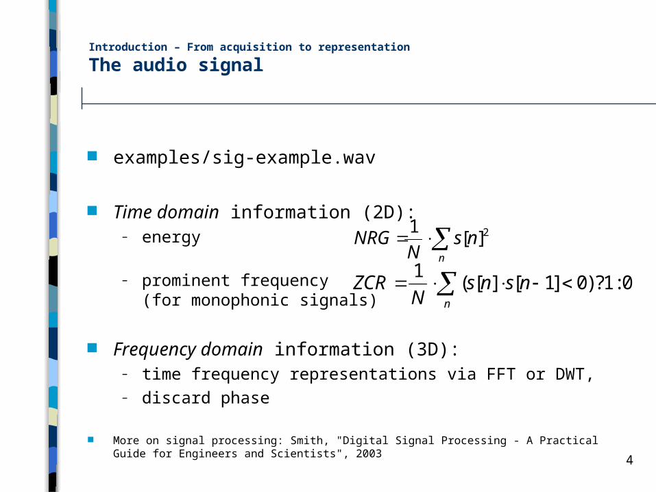
Time domain information (2D): – energy
– prominent frequency (for monophonic signals)
Frequency domain information (3D): – time frequency representations via FFT or DWT, – discard phase
More on signal processing: Smith, "Digital Signal Processing - A Practical Guide for Engineers and Scientists", 2003 4
Introduction – From acquisition to representation
The audio signal
examples/sig-example.wav
n
nsN
NRG 2][1
n
nsnsN
ZCR 0:1?)0]1[][(1
5
Introduction – From signal to features
Frame-based Processing (1)
Feature extraction: – Reduction in overall information – while maintaining or even emphasizing the useful
information
Audio signal: – Neither stationary
• (=> problem with transformations like DFT when viewed as a whole)
– nor conveys its meaning in single samples
chop into short, usually overlapping chunks called frames extract features per frame

6
Introduction – From signal to features
Frame-based Processing (2)
Prominent parameters: – 16ms frame-step, – 32ms frame-size (50% overlap)
Technically: double-matrix f[y][x], y=row-count, x=feature-dimension
))(
(1frameStep
frameSizetsampleCounceilfloory

7
Introduction – From signal to features
Feature example: Mel Frequency Cepstral Coefficients
MFCC: A compact representation of a frame’s smoothed spectral shape– Preemphasize: s[n] = s[n] – α*s[n-1]
(boost high frequencies to improve SNR; α close to 1)– Compute magnitude spectrum: |FFT(s[n])|– Accumulate under triangular Mel-scaled filter bank
(resembles human ear) – Take DCT of filter bank output, discard all coefficients > M
(i.e. low-pass) Low-pass filtered Spectrum of a spectrum: "Cepstrum“
MFCCs convey most of the useful information in a speech or music signal, but no pitch information
8
Introduction – Audio segmentation
Content of audio signals
The sample-array is 1D
nevertheless sound carries information in many different layers or "dimensions“– Silence non-silence– Speech music noise– Voiced speech unvoiced speech– Different musical genres, speakers, dialects, linguistical
units, polyphony, emotions, . . .
Segmentation: separate one ore more of the above types from each other by more or less specialized algorithms

9
Introduction – Audio segmentation
Typical approaches to segmentation
Classification: – build models for each type a priori, – test which fits best for a given chunk of frames
(Statistical) change point detection: – Find changes in feature distribution parameters
Local – (sliding window based)
Global – (genetic algorithms, Viterbi segmentation)
10
Audio type classification – The algorithm by Lu et al.
Algorithmic Overview
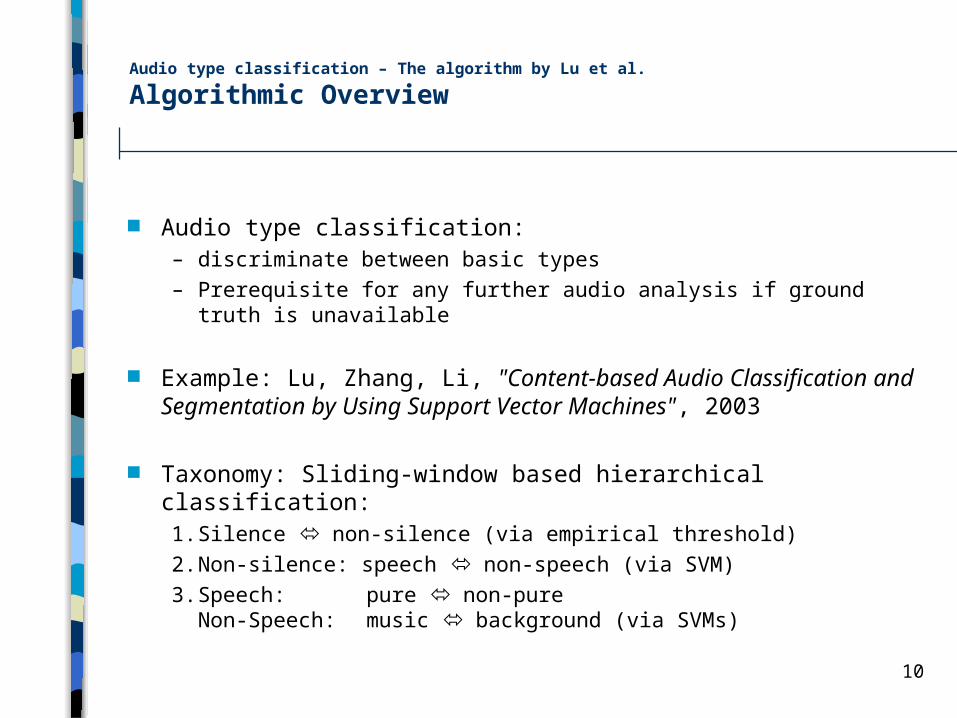
Audio type classification: – discriminate between basic types– Prerequisite for any further audio analysis if ground truth is
unavailable
Example: Lu, Zhang, Li, "Content-based Audio Classification and Segmentation by Using Support Vector Machines", 2003
Taxonomy: Sliding-window based hierarchical classification:1. Silence non-silence (via empirical threshold)2. Non-silence: speech non-speech (via SVM)3. Speech: pure non-pure
Non-Speech: music background (via SVMs)

11
Audio type classification – The algorithm by Lu et al.
Used features (1)
Use 7+1 different features to cope with diverse signal properties– NRG
(for silence detection alone, together with ZCR: both must be smaller than a threshold)
– ZCR– 8 MFCCs
– Sub band Power (ratio of power in each of 4 sub bands to overall power)
– Brightness and Bandwidth (frequency centroid and spectral spread width)

12
Audio type classification – The algorithm by Lu et al.
Used features (2)
– Spectrum Flux (average spectral variation between two successive frames)
– Band Periodicity (periodicity in 4 sub bands:
– Noise Frame Ratio (ratio of noisy frames in a sub-clip, i.e. frames with no prominent periodicity)
12
1,2
1
4
1,4
1
8
1,8
10

13
Audio type classification – The algorithm by Lu et al.
Feature construction
Sliding window is here called a sub-clip
What is a representative feature vector of such a sub-clip?– remember: a 1D array or a single row in a matrix
Aggregate frame-based features per sub-clip (1s long):1. Concatenate (columns of) different feature vectors to one big
vector2. Compute mean µ and standard deviation σ of these vectors
in each sub-clip
Feature vector of one sub-clip: concatenated and of each individual feature
14
Audio type classification – The algorithm by Lu et al.
At runtime (1)
Train algorithm – (huge annotated data corpus needed, e.g. 30h)
– Find suitable thresholds on NRG and ZCR for silence detection
– Train SVMs for each pair to discriminate between
Training runtime: approx. 1 week

15
Audio type classification – The algorithm by Lu et al.
At runtime (2)
Test it– preclassify single frames as silence– for each sub-clip do . . .
• extract and aggregate and normalize features• classify them using SVM tree
– smooth the label series l[i]: IF (l[i+1]!=l[i] AND l[i+2]!=l[i+1] AND l[i+1]!=SILENCE) THEN l[i+1]=l[i]
– store result for all non-silence frames (silence stored before)
Implementation effort: approx. 3 month
16
Audio type classification – The algorithm by Lu et al.
Experimental results
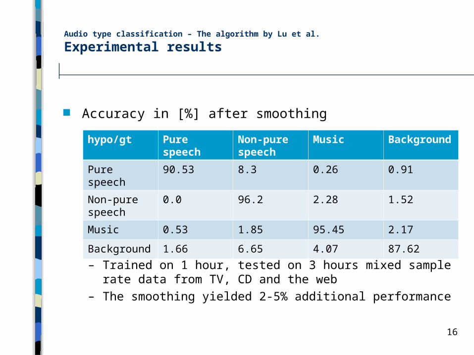
Accuracy in [%] after smoothing
– Trained on 1 hour, tested on 3 hours mixed sample rate data from TV, CD and the web
– The smoothing yielded 2-5% additional performance
hypo/gt Pure speech
Non-pure speech
Music Background
Pure speech 90.53 8.3 0.26 0.91
Non-pure speech
0.0 96.2 2.28 1.52
Music 0.53 1.85 95.45 2.17
Background 1.66 6.65 4.07 87.62
17
Speaker change detection – The algorithm by Kotti et al.
What is speaker change detection?
Take a speech-only audio stream – i.e. do ATC and discard all non-speech frames
Find all change points, – i.e. all samples spoken by a speaker different from the
speaker of the previous sample
Example: Kotti, Benetos, Kotropoulos, "Computationally Efficient and Robust BIC-Based Speaker Segmentation", 2008
Taxonomy: (adaptive) sliding window based statistical cp. detection

18
Speaker change detection – The algorithm by Kotti et al.
The basic idea: BIC (1)
Take a chunk of frames (Z) and divide it into two chunks X, Y – (not necessarily half-way)
Model X, Y and Z each with a multivariate Gaussian, – i.e estimate µ and Σ for each
Compute log likelihood L of each (sub-)chunk given its model, – i.e. for a chunk A: )()'(
2
1log2
1)2log(
21
1 AnA
A
n AnAA aad
AL
19
Speaker change detection – The algorithm by Kotti et al.
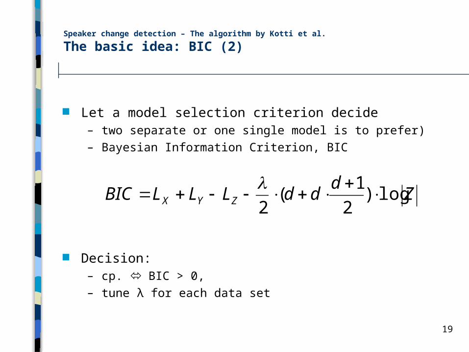
The basic idea: BIC (2)
Let a model selection criterion decide– two separate or one single model is to prefer)– Bayesian Information Criterion, BIC
Decision: – cp. BIC > 0, – tune λ for each data set
Zd
ddLLLBIC ZYX log)2
1(
2
20
Speaker change detection – The algorithm by Kotti et al.
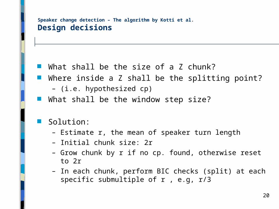
Design decisions
What shall be the size of a Z chunk? Where inside a Z shall be the splitting point?
– (i.e. hypothesized cp) What shall be the window step size?
Solution:– Estimate r, the mean of speaker turn length– Initial chunk size: 2r– Grow chunk by r if no cp. found, otherwise reset to 2r– In each chunk, perform BIC checks (split) at each specific
submultiple of r , e.g, r/3

21
Speaker change detection – The algorithm by Kotti et al.
What about features? (1)
MFCCs are often applied to SCD problems, – but dimensionality and parameters vary greatly
Idea:– Fix frame- and DSP-parameters to some common standard– Use upper bound of dimensionality (36) and find the best
subset comprising reasonable amount of dimensions (24)– Add δ and δδ coefficients to the final subset

22
Speaker change detection – The algorithm by Kotti et al.
What about features? (2)
Feature (subset) selection:– Create a training data set:
• files containing one cp. and • files containing no cp.
– Define a performance measure J– Find best 24-dimensional subset according to it
– 24-dimensional subsets possible
need heuristic strategy
700.677.251.124
36

23
Speaker change detection – The algorithm by Kotti et al.
Feature selection algorithm: details
Use depth-first search branch & bound search strategy – (i.e. with backtracking)– Search tree has 36-24+1 = 13 levels
Traverse the tree, – skip branches that have lower J then the so far seen best
performance for the current level
– Sw is within class scatter: deviation of sample vectors from their respective class means
– Sb is between class scatter: deviation of sample vectors from the gross (overall, combined) mean
)( 1bW SStrJ
24
Speaker change detection – The algorithm by Kotti et al.
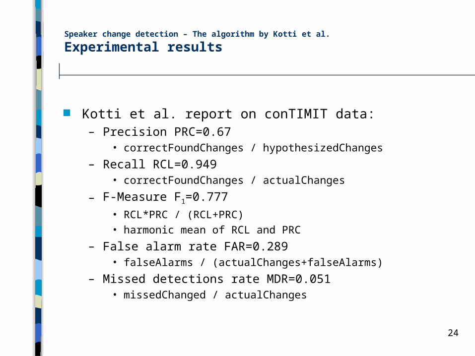
Experimental results
Kotti et al. report on conTIMIT data:– Precision PRC=0.67
• correctFoundChanges / hypothesizedChanges
– Recall RCL=0.949 • correctFoundChanges / actualChanges
– F-Measure F1=0.777 • RCL*PRC / (RCL+PRC)• harmonic mean of RCL and PRC
– False alarm rate FAR=0.289 • falseAlarms / (actualChanges+falseAlarms)
– Missed detections rate MDR=0.051• missedChanged / actualChanges

25
Speaker change detection – General considerations
Literature survey result: what makes a good SCD algorithm? (1)
Do multi step analysis, reduce FAR in each step Use area surrounding a cp., e.g. self-similarity-matrix for
continuity-signal – (maybe as a last step?)
Employ a method that treats the stream holistically – (e.g. Viterbi resegmentation, GA)
Use complementary features, also on different levels Fuse different classifiers already in each step Create multiple chances for a cp. to get detected
26
Speaker change detection – General considerations
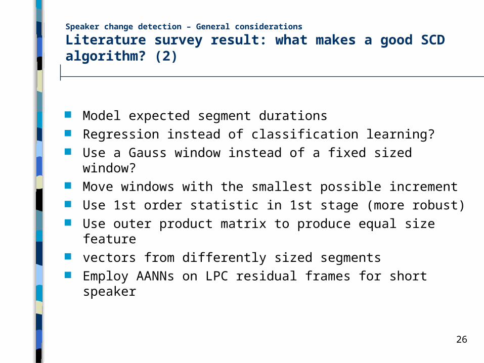
Literature survey result: what makes a good SCD algorithm? (2)
Model expected segment durations Regression instead of classification learning? Use a Gauss window instead of a fixed sized window? Move windows with the smallest possible increment Use 1st order statistic in 1st stage (more robust) Use outer product matrix to produce equal size feature vectors from differently sized segments Employ AANNs on LPC residual frames for short speaker
27
Speaker change detection – General considerations
The end.
Thank you for your attention!


![Home [demo.jumpbox.ch] · Web viewEin Worddokument als Muster für Ihre Webseite. DEUTSCH docx docx docx Author internezzo ag - Priska Stadelmann Created Date 09/30/2015 01:19:00](https://static.documents.pub/doc/80x56/60b181b622c4ae54e51770b5/home-demo-web-view-ein-worddokument-als-muster-fr-ihre-webseite-deutsch-docx.jpg)

![Volume XLIV September Number 4 · THE HEBREW CONCEPTION OF THE WORLD. By Luis I. ]. Stadelmann. Rome: Pontifical Biblical Institute, 306 BOOK REVIEW 1970. 207 pages. Paper. 2,850](https://static.documents.pub/doc/80x56/5ea96edca11cf62f9207ca3e/volume-xliv-september-number-4-the-hebrew-conception-of-the-world-by-luis-i-.jpg)


