NBER WORKING PAPER SERIES

WAGING WAR ON POVERTY:HISTORICAL TRENDS IN POVERTY USING THE SUPPLEMENTAL POVERTY MEASURE

Liana FoxIrwin GarfinkelNeeraj KaushalJane Waldfogel

Christopher Wimer

Working Paper 19789http://www.nber.org/papers/w19789

NATIONAL BUREAU OF ECONOMIC RESEARCH1050 Massachusetts Avenue

Cambridge, MA 02138January 2014

We are grateful for funding support from the Annie E. Casey Foundation and from the National Instituteof Child Health and Human Development (NICHD) through grant R24 HD058486-03 to the ColumbiaPopulation Research Center (CPRC). We benefited from research assistance from Madeleine Gelblum,Nathan Hutto, and Ethan Raker. We are also grateful to seminar participants at CPRC and RussellSage Foundation, as well as many colleagues who provided helpful insights and advice, in particular,Jodie Allen, Ajay Chauhdry, Sheldon Danziger, Daniel Feenberg, Gordon Fisher, Thesia Garner, DavidJohnson, Mark Levitan, Trudi Renwick, Kathy Short, and Tim Smeeding. The views expressed hereinare those of the authors and do not necessarily reflect the views of the National Bureau of EconomicResearch.

NBER working papers are circulated for discussion and comment purposes. They have not been peer-reviewed or been subject to the review by the NBER Board of Directors that accompanies officialNBER publications.

© 2014 by Liana Fox, Irwin Garfinkel, Neeraj Kaushal, Jane Waldfogel, and Christopher Wimer. Allrights reserved. Short sections of text, not to exceed two paragraphs, may be quoted without explicitpermission provided that full credit, including © notice, is given to the source.

Waging War on Poverty: Historical Trends in Poverty Using the Supplemental Poverty MeasureLiana Fox, Irwin Garfinkel, Neeraj Kaushal, Jane Waldfogel, and Christopher WimerNBER Working Paper No. 19789January 2014JEL No. I32

ABSTRACT

Using data from the Consumer Expenditure Survey and the March Current Population Survey, wecalculate historical poverty estimates based on the new Supplemental Poverty Measure (SPM) from1967 to 2012. During this period, poverty as officially measured has stagnated. However, the officialpoverty measure (OPM) does not account for the effect of near-cash transfers on the financial resourcesavailable to families, an important omission since such transfers have become an increasingly importantpart of government anti-poverty policy. Applying the SPM, which does count such transfers, we findthat historical trends in poverty have been more favorable than the OPM suggests and that governmentpolicies have played an important and growing role in reducing poverty --- a role that is not evidentwhen the OPM is used to assess poverty. We also find that government programs have played a particularlyimportant role in alleviating child poverty and deep poverty, especially during economic downturns.

Liana FoxSwedish Institute for Social ResearchStockholms UniversitetSE-106 91 Stockholmliana.fox@sofi.su.se

Irwin GarfinkelColumbia UniversitySchool of Social Work1255 Amsterdam AvenueNew York, NY 10027ig3@columbia.edu

Neeraj KaushalColumbia UniversitySchool of Social Work1255 Amsterdam AvenueNew York, NY 10027and NBERnk464@columbia.edu

Jane WaldfogelColumbia UniversitySchool of Social Work1255 Amsterdam AvenueNew York, NY 10027jw205@columbia.edu

Christopher Wimer1255 Amsterdam AvenueOffice 735New York, NY 10027cw2727@columbia.edu

3

Introduction

This year marks the 50th

anniversary of the War on Poverty. So it is an appropriate time to look

at historical trends in poverty and the role government has played in combating poverty. While

much has been written on this topic, we provide the first estimates of historical trends in poverty

and the role of government anti-poverty policies using an improved measure of poverty known

as the supplemental poverty measure (SPM). Our analyses cover the period 1967-2012.

The SPM came about because of widespread agreement among analysts, advocates, and

policymakers that the official U.S. poverty measure is inadequate. As documented by the

National Academy of Sciences (NAS) in their landmark 1995 report (Citro and Michael, eds.,

1995) , the official poverty measure (OPM) understates the extent of poverty by using thresholds

that are outdated and may not adjust appropriately for the needs of different types of individuals

and households, in particular, families with children and the elderly. At the same time, it

overstates the extent of poverty, and understates the role of government policies, by failing to

take into account several important types of government benefits (in particular, the Supplemental

Nutrition Assistance Program/Food Stamps and tax credits), which are not counted in cash

income (Smeeding, 1977; Blank, 2008). Because of these (and other failings), official poverty

statistics do not depict an accurate picture of poverty or the role of government policies in

combating poverty.1

Developing an improved poverty measure is a complex undertaking. The NAS panel devoted a

good deal of attention to this challenge, and their recommendations for developing a new

measure were widely endorsed. The NAS recommendations were used by the Census Bureau for

several years to generate alternative poverty statistics on an experimental basis. They also

provided the basis for state and local efforts to define poverty in a more accurate way; one of the

earliest and most ambitious of these efforts is the work undertaken by Mark Levitan and

colleagues at the NYC Center for Economic Opportunity, which resulted in a series of reports

using an alternative poverty measure.2

The move toward an improved poverty measure took a great leap forward a few years ago with

the release by the Census Bureau of poverty estimates using a new supplemental poverty

measure (SPM) (Short, 2011). While Census had previously released alternative poverty

statistics drawing on a variety of experimental measures, this was the first time it produced

figures using a single preferred alternative measure, the SPM. These new estimates (and those in

2 successor reports; Short, 2012, 2013) demonstrate how using an improved measure of poverty

alters our understanding of poverty and the role of government programs in reducing poverty.3

1 See also Bernstein, 2001; Blank and Greenberg, 2008; Hutto et al., 2011; Iceland, 2005).

2 The most recent is NYC Center for Economic Opportunity (2013). See also Levitan et al. (2010) for an overview

of their approach. Other state and local efforts have followed in Wisconsin (Smeeding et al., 2013), Massachusetts,

Illinois, and Georgia (Wheaton et al., 2011), California (Bohn et al., 2013), and Virginia (Cable, 2013). 3 The SPM has been widely but not universally endorsed. Many analysts question its inclusion of medical out of

pocket expenditures (an item the NAS panel failed to reach agreement on) (see e.g. Korenman and Remler, 2012).

Meyer and Sullivan (2003, 2011, 2012c) note several ways in which the SPM is an improvement over the OPM, but

argue that a consumption-based measure would be superior to both the SPM and OPM. However, as Hoynes (2012)

points out, a consumption-based measure cannot be used to produce counter-factual estimates along the lines of

those we produce here.

4

From the Census reports, we know that moving to SPM results in a higher overall threshold,

more resources, but also more expenses. The net effect is a slightly higher overall poverty rate –

16.0 percent with SPM vs. 15.1 percent with OPM in 2012 – with poverty lower under SPM than

OPM for children (18.0 percent vs. 22.3 percent) but higher under SPM than OPM for seniors

(14.8 percent vs. 9.1 percent) (Short, 2013).4 The Census reports also illustrate the crucial anti-

poverty role played today by programs not counted under the OPM (programs such as

SNAP/Food Stamps and EITC).

However, the Census reports provide SPM estimates for 2009-2012 only and therefore cannot

tell us how using an SPM-like measure would alter our understanding of historical trends in

poverty and the role of government policies in reducing poverty. To address that question, we

estimate an SPM-like poverty measure historically.

Specifically, making use of historical data from the Annual Social and Economic Supplement to

the Current Population Survey (March CPS) and the Consumer Expenditure Survey (CEX), we

produce SPM estimates for the period 1967 to 2012.5 As described in greater detail below, we

produce our SPM series using a methodology similar to that used by the Census in producing

their SPM estimates, but with adjustments for differences in available historical data. We first set

poverty thresholds based on consumer expenditures on food, clothing, shelter, and utilities

(FCSU) between the 30th

-36th

percentiles of expenditures on FCSU, plus an additional 20 percent

to account for additional necessary expenditures. Thresholds are further adjusted depending on

whether the household makes a mortgage or rent payment, or if the household owns its home

free and clear of a mortgage. These thresholds are based on 5-year rolling averages of the CEX

data when available (and on averages from fewer years when data for the previous five years are

not available).6 Thresholds are then applied to the March CPS sample using an equivalization

process that weights adults and children based on standard theories of consumption and

economies of scale. Rather than comparing the threshold to only pre-tax income as is done in the

OPM, the threshold is compared to a much broader set of resources, including post-tax income

and near-cash transfers (such as SNAP/Food Stamps), and then subtracting work, child care, and

medical out-of-pocket expenditures. This process is then repeated historically.

To briefly preview the results, we find that historical trends in poverty have been more favorable

than the OPM suggests and that government policies have played an important and growing role

in reducing poverty --- a role that would not be evident if we only used the OPM to assess

poverty. This can be seen most clearly in our SPM “counterfactual” analyses – where we show

poverty rates both with and without taking key government programs into account. These

counterfactual estimates provide an accounting of how much taking government taxes and

4 Short 2013 uses a modified version of the official poverty measure, which includes unrelated individuals under age

15. This results in slightly different OPM numbers for the Short paper compared with official statistics: overall (15.1

vs 15.0) and children (22.3 vs 21.8). 5 Although March CPS data exist for earlier years, limitations with those data prevent us from using the CPS to

estimate the SPM earlier than 1967. In work in progress, we are exploring using the 1960 Census to provide data on

poverty for 1959. 6 In a related paper (Wimer et al., 2013a) we deviate from the Census’ calculation of relative poverty thresholds and

present analyses where the poverty threshold is anchored or fixed at a specific point in time. This transforms the

poverty measure into an absolute poverty standard, more similar to how the OPM thresholds are calculated over

time.

5

transfers into account alters our estimates of poverty. Because we do not model potential

behavioral responses to the programs, our estimates do not tell us what actual poverty rates

would have been in the absence of the programs. Instead, they provide static or short-run

estimates of the impact of programs ignoring behavioral responses.7

These counterfactual analyses show that government policies have significantly reduced the

share of the population in poverty, and the share in deep poverty, throughout the 45 year period

we examine, and with especially pronounced effects during economic downturns, in particular,

during the recent Great Recession.8 Overall, we find that in the absence of government benefits,

the poverty rate would have risen from 25 percent to 31 percent from 1967 to 2012, instead of

falling from 19 percent to 16 percent. So in 2012, government programs reduced poverty by 15

percentage points – nearly half of its pre-transfer level -- up from a reduction of 6 percentage

points -- about a quarter of its pre-transfer level -- in 1967.

Data and Methods

Constructing a historical SPM in the Current Population Survey (CPS) requires construction of

“poverty units,” estimation of poverty thresholds, and calculation of resources and non-

discretionary expenses. We describe our approach to units, thresholds, resources, and expenses in

turn.

Poverty Units

The “poverty unit,” or those who are thought to share resources, is defined as the family under

the OPM (i.e. all related individuals, including sub-families residing in the same household). The

SPM departs from this definition to include a broader set of individuals. In particular, families

are broadened to include unmarried partners (and their children/family members), unrelated

children under age 15, and foster children under age 22 (when identifiable). We therefore first

create SPM poverty units in the CPS in all years back to 1967. Details on these procedures are

provided in the technical appendix. All resources and non-discretionary expenses are pooled

across members of the poverty unit to determine poverty status.

Poverty Thresholds

From 1984-2012, we follow the Census Bureau methodology in constructing poverty thresholds

using five-year rolling averages of the Consumer Expenditure Survey (CEX) data on out-of-

pocket expenditures on food, clothing, shelter and utilities (FCSU) by consumer units with

exactly two children (called the “reference unit”). All expenditures by consumer units with two

children are adjusted by the three-parameter equivalence scale, (described in the appendix; see

also Betson and Michael, 1993) and then ranked into percentiles. The average FCSU for the 30-

7 In this respect, our estimates are similar to the “zeroing out” exercise undertaken by Bitler and Hoynes (2013) in

their analysis of the role of the safety net in the Great Recession. Our analysis differs from theirs in using the SPM,

whereas they use an SPM-like measure of income alongside OPM thresholds. The time period also differs – their

focus is 1980 to the present whereas our analysis goes back to 1967. 8 Meyer and Sullivan (2012a and b) reach a similar conclusion in their historical analysis using a consumption-based

measure of poverty – although their methodology differs from ours, they also find that the OPM time series

understates progress in reducing poverty since the War on Poverty.

6

36th percentile of FCSU expenditures is then multiplied by 1.2 to account for additional basic

needs. We then use equivalence scales to set thresholds for all family configurations.

It is important to note that Census previously defined the reference unit as consumer units with

two adults and two children but changed this methodology given the fact that, because of family

change, two-adult, two-child units have tended to become a more select and affluent group over

time (see Garner, 2010 for more detail on the development of SPM poverty thresholds). We

explore the effects of this methodological choice in Appendix Figure A1, which shows that the

thresholds would have been higher had we focused on a fixed two-adult, two-child family unit.

However, we choose to be consistent with current Census recommendations.9

We determine thresholds overall, and by housing status. The Census Bureau produces base

thresholds for three housing status groups: owners with a mortgage; owners without a mortgage;

and renters. The SU portion of the FCSU is estimated separately for each housing status group.

Our overall SPM threshold is simply the average SU for all consumer units in the 30-36th

percentile of FCSU. Note that an overall SPM threshold is not advised or published by OMB. In

creating an overall SPM threshold, our objective is to facilitate a historical comparison of OPM

with a single SPM. However, in estimating poverty rates, each poverty unit is assigned a housing

status specific threshold—no family receives the overall threshold. We discuss this issue further

in the results section.

The annual CEX series does not go back beyond 1980 except for two sets of surveys in 1960/61

and 1972/73. Thus, our thresholds for 1980-1983 are based on fewer than five years of data.

Specifically, we use four years of data (1980-1983) to construct the 1983 threshold, three years

to construct the 1982 threshold, two years of data to construct the 1981 threshold, and just 1 year

of data to construct the 1980 threshold. To construct thresholds in the years prior to 1980, we

follow the same methodology, but instead of using five-year averages, we estimate thresholds in

1961 and 1972/73 and interpolate the intermediate years of 1962-1971 and 1974-1979 using the

rate of change in the CPI-U. 10

Despite our best efforts to create a historically-consistent series, due to changes in CEX data

design, our thresholds are not entirely consistent over time. In 1982/83, the CEX was only

representative of urban areas. Inclusion of these inconsistent years will affect estimates from

1982-1987. However, based on an analysis of 1980-1991 data, we believe the magnitude of the

bias to be small (less than 5 percent). Additionally, the 1972/73 CEX only includes consumer

units who participated in all four interviews, while in other years, all consumer units, regardless

of the number of interviews they participated in, were included in the threshold estimations. Thus

our thresholds will be affected by any systematic attrition.

9 The effect of the family composition change (i.e. the rising share of two child families headed by single parents) is

somewhat muted because the CEX under-represents single parent families (because it fails to identify some single

parent families co-residing in extended family households). 10

Because the 1960 portion of the 1960-61 CEX contains only urban consumer units, we create a threshold for 1961

using just the 1961 portion of that dataset. For 1972/73, we treat the data as we do in 1981, using both years to

generate a 1973 data point.

7

Resources

The SPM differs from the OPM in taking into account a fuller set of resources including near-

cash and in-kind benefits, as well as tax credits. We describe below how we calculate the value

of these various types of resources.

SNAP/Food Stamps: Receipt of the Supplemental Nutrition Assistance Program (SNAP),

formerly known as the Food Stamp Program, is routinely measured in the CPS beginning in 1980

(for calendar year 1979). The program, however, existed for all years included in our analysis

(albeit on a very small scale in our earliest years). It grew rapidly over the 1970s as it was

extended nationally, making it important to capture SNAP/Food Stamps benefits prior to 1979 in

our historical SPM measure. We use a 2-step procedure to impute SNAP/Food Stamps for the

earlier years: each household in the CPS is first predicted to receive or not receive SNAP/Food

Stamps, followed by imputation of the benefit amount for those predicted to receive the program.

The procedure for imputation is based on administrative data on SNAP/Food Stamps caseloads

and benefit levels and is detailed in the technical appendix.

School Lunch Program: The National School Lunch Act of 1946 launched a federally assisted

meal program that provides free or low-cost lunches to children in public and nonprofit private

schools. Like SNAP/Food Stamps, however, it is only measured in the CPS starting in 1980 (for

calendar year 1979). We impute the value of the School Lunch Program benefits using a

procedure similar to SNAP/Food Stamps imputation. Details of our imputation approach are in

the technical appendix.

Women Infants and Children (WIC): The WIC program, which provides coupons that can be

used to purchase healthy food by low-income pregnant women and women with infants and

toddlers, was established as a pilot program in 1972 and became permanent in 1974, with large

expansions occurring in the 1970s. While the CPS does not provide data on the value of WIC,

since 2001 it has included data on the number of WIC recipients per household. Therefore, a

procedure was necessary to impute participation in WIC prior to 2001 and the value of WIC for

all years. Details of our imputation approach can be found in the technical appendix.

Housing Assistance: Federal housing assistance programs have existed in the United States since

at least the New Deal. Such programs typically take one of two forms: reduced-price rental in

public housing buildings or vouchers that provide rental assistance to low-income families

seeking housing in the rental market. In the CPS, questions asking about receipt of these two

types of housing assistance exist back to 1976 (for calendar year 1975). This means housing

assistance receipt for years prior to 1975 must be imputed. Unlike programs like SNAP/Food

Stamps, we only need to impute receipt of assistance. To estimate the value of the assistance, we

first estimate rental payments as 30 percent of household income, and subtract this from the

shelter portion of the threshold. We then apply a small correction factor given that this valuation

will tend to overestimate the value of housing assistance relative to Census procedures, which

are able to utilize rich administrative data in the modern period. Further detail on both the

imputation procedure and the benefit valuation are in the technical appendix.

8

Low Income Home Energy Assistance Program (LIHEAP): LIHEAP was first authorized in

1980 and funded in 1981. It is measured in the CPS starting in 1982 (for calendar year 1981).

Thus, the entire history of the program is captured in the CPS, and no imputations were

necessary for this program.

Taxes and Tax Credits: Like with SNAP/Food Stamps and the School Lunch Program, the

Census’ official tax model, and resultant after-tax income measures, does not exist in the CPS

prior to 1980 (for calendar year 1979). The EITC, however, was enacted in 1975 (albeit in a

much smaller form than it exists today). The Child Tax Credit provides additional benefits to

families with children, and was created in 1997. And income and payroll taxes have obviously

existed for much longer. Thus, it was necessary to develop after-tax income measures in years

prior to 1980. We used the National Bureau of Economic Research’s Taxsim model (Feenberg

and Countts, 1993) to estimate these after-tax income variables. Full details on the tax model we

built are provided in the technical appendix.

Non-Discretionary Expenses

Aside from the payroll and income taxes paid that are generated from the tax model, the SPM

also subtracts medical out-of-pocket expenses (MOOP) from income, as well as capped work

and child care expenses. MOOP and child care expenses are directly asked about in the CPS only

starting in 2010, meaning we must impute these expenses into the CPS for virtually the whole

period. For consistency, we use data from the CEX to impute MOOP and child care expenses

into the CPS for all years. Work expenses (e.g., commuting costs) are never directly observed in

the CPS and are currently estimated based on the Survey of Income and Program Participation

(SIPP). We estimate work expenses back in time to 1997 using an extended time series provided

to us by the Census Bureau. For years prior to that, we used a CPI-U inflation-adjusted value of

the 1997/98 median work expenditures. Further details on the imputation of medical, work, and

child care expenses are provided in the technical appendix.

Results

This section presents our historical SPM time series back to 1967, just after the launch of the

War on Poverty. We first show how our SPM thresholds compare to the OPM thresholds and

then present how our SPM poverty rates compare to the official published OPM poverty rates,

both overall and for three broad age groups: children (those under age 18); working-age adults

(age 18-64); and the elderly (aged 65 and above).

In our main analysis, we examine how government policies and programs affect poverty rates,

using our SPM time-series to calculate a set of counterfactual estimates -- showing what poverty

rates would be with and without taking into account specific anti-poverty policies. We focus in

this section on overall poverty rates as well as child poverty rates – the latter given that many

anti-poverty programs are explicitly targeted toward families with children.

9

Poverty Thresholds: 1967-2012

Figure 1 shows the value of our estimated SPM poverty thresholds for 1967-2012 (in nominal

dollars), and how they compare to the OPM thresholds for the same years.11

For illustrative

purposes, the thresholds displayed in the figure are for two-adult two-child families. The SPM

and OPM thresholds track one another fairly closely over time until about 2000. Beginning in

2000 the two thresholds begin to diverge rather markedly, with SPM thresholds overtaking and

outpacing the OPM thresholds. By 2012, the thresholds are roughly $1,800 apart.

Why are the thresholds so similar for such a long period of time? Evidently, the growth in

expenditures on FCSU at the 30th

-36th

percentile of the FCSU distribution tracks very closely to

the growth in the OPM thresholds (i.e. their adjustment for changes in the cost of living). As

discussed earlier (and shown in Appendix Figure 1), it is also clear that basing the threshold on

expenditures of all two-child families, rather than two-adult two-child families, has tempered the

growth in SPM thresholds because they are based on increasingly less affluent families as the

composition of two-child families has shifted to include more single parents who have lower

incomes.12

Why do the thresholds diverge in the 2000s? To address this question, we looked at each

component of the SPM threshold from 1967 to the present. Shelter expenditures have been rising

steadily over time, and only in the most recent couple of years have declined a bit, using

multiyear averages. Prior to 2000, the rise in housing cost is accompanied by a decline in

expenditures on food. From 2000 onwards, housing costs begin to grow faster and the declining

trend in food cost is reversed. Together, then, we believe that the housing bubble along with the

uptick in food costs largely explain the divergence in OPM and SPM thresholds in recent years.13

It is important to keep in mind, however, that part of the reason the thresholds do not diverge

even more is because of the selection of all consumer units with two children as the reference

unit, as discussed above.

It may seem at first a bit of a puzzle that SPM thresholds did not come down during the Great

Recession. However, it is worth remembering that the SPM thresholds are based on five years of

data, meaning the point estimate for, say, 2009, is based on data from 2005 to 2009, and thus will

include two to three years of the housing bubble that preceded the Great Recession. It is also

11

As mentioned earlier, Census and the BLS do not produce overall SPM thresholds, but only thresholds that vary

by housing status. We present an overall threshold here so that we can compare the average SPM threshold to the

OPM one. However, all SPM poverty rates are calculated using the housing status-relevant SPM thresholds, not the

overall ones. 12

To some extent, the similarity in the OPM thresholds and our SPM thresholds prior to 1980 is because our

thresholds for this period are interpolated, but the proximity between the two thresholds continues throughout the

1980s and 1990s, when our SPM thresholds are based only on actual CEX expenditures. 13

Appendix Figure 2 displays SPM thresholds by housing status, again compared to OPM thresholds. The

divergence between the overall SPM thresholds and OPM thresholds observed in Figure 1 stems from a rise in all

three groups’ SPM thresholds. In supplemental analysis we found some change over time in the relative share of

Americans in each of the three groups, with an overall decline in the proportion owning their home with no

mortgage. This means that the SPM thresholds are not only pulling away from the OPM threshold in recent years

because of rising expenditures on housing (as discussed), but also a shift of population into the higher-spending

categories.

10

possible that because the components of the SPM thresholds (food, clothing, shelter, and

utilities) are a basic bundle of “necessities,” they may be less susceptible to large economic

shocks than overall spending would be. Nevertheless, it will be illuminating to watch trends in

the SPM thresholds in coming years, when the five-year moving averages will be more heavily

dominated by the years of the Great Recession and its aftermath.

SPM versus OPM Poverty Rates

Figure 2 presents our overall time series of poverty rates for the SPM and OPM. In the

aggregate, our estimated SPM poverty rates are consistently higher than OPM poverty rates,

although generally the difference is small, roughly 1-3 percentage points. In 1967, the SPM

poverty rate is 5.1 percentage points higher than the OPM rate and the gap narrows over time,

especially during the late 1990s when the gap shrinks to about a half a percentage point. After

2000, as the SPM thresholds begin to pull away from OPM thresholds and following the mild

recession of the early 2000s, the SPM and OPM poverty rates begin to diverge again. By 2012,

the SPM is only 1 percentage point higher than the OPM.

These overall poverty rates mask considerable heterogeneity across the population. In Figures

3a-3c, we show OPM and SPM poverty rates for three age groups: children; working-age adults;

and the elderly. The overall OPM and SPM trends are mirrored in the trend for the largest group,

working-age adults (shown in Figure 3b), but the story is somewhat different for children and the

elderly. As can be seen in Figure 3a, child poverty rates under the SPM are not consistently

above or below the OPM child poverty rates. The Census’ SPM analyses show that in the past

few years, the child poverty rate under the SPM is lower than under the OPM because the former

counts many more benefits targeted at families with children (Short, 2013). But Figure 3a shows

that this has not always been the case.

Figure 3c provides another interesting story masked by the overall trends. For the elderly, OPM

and SPM poverty rates both plummet in the 1970s, which probably reflects the expansions of the

Social Security program that happened starting in the early 1970s (Englehardt and Gruber,

2006). But while the OPM poverty rate for the elderly continues drifting downward after 1980,

the SPM poverty rate for the elderly first levels off and then begins rising after 2001. As

mentioned, the SPM subtracts medical out-of-pocket (MOOP) expenses from resources, a

decision that is especially consequential for elderly poverty rates. So, if medical care is getting

more expensive over this period, then that could explain the fanning out of SPM and OPM rates

we see in Figure 3c. However, supplemental analyses revealed that this was only partially the

case. In addition to increasing MOOP expenses, two other factors combined to explain the

divergence we see starting in the 1980s: the relative decline in the share of the elderly who own

their home without a mortgage (and thus face a lower poverty threshold); and the general

increase in SPM poverty thresholds in the 2000s. Many elderly individuals have incomes that

hover just above the OPM threshold, so the combination of gradually higher thresholds, as well

as the subtraction of medical expenses, results in the fanning out of SPM vs. OPM elderly

poverty rates that we see in Figure 3c.

11

The Role of Government Programs

A major advantage of the SPM, compared to the OPM, is that the SPM takes into account the full

array of government transfers and thus allows for a more comprehensive accounting of the role

of government programs in combating poverty. In this section, we make use of the SPM to

calculate a set of counterfactual estimates for what poverty rates would look like if we did not

take government transfers into account. We note again that these counterfactual estimates tell us

in an accounting sense how much taking government transfers into account alters our estimates

of poverty. Because we do not model potential behavioral responses to the programs, these

estimates cannot tell us what actual poverty rates would be in the absence of the programs.

However, as documented in many previous studies the aggregate effect of these behavioral

responses is likely to be small.14

We begin by considering the income-to-needs distribution of the population, with and without

government transfers (in Figures 4a and 4b respectively). We construct two resource measures,

total SPM resources and SPM resources minus all government transfers. These transfers include:

food and nutrition programs (SNAP/Food Stamps, School Lunch, WIC); other means tested

transfers (SSI, cash welfare (i.e. TANF/AFDC), Housing Subsidies, EITC,15

LIHEAP); and

social insurance programs (Social Security, Unemployment Insurance, Worker’s Compensation,

Veteran’s Payments, and government pensions16

).

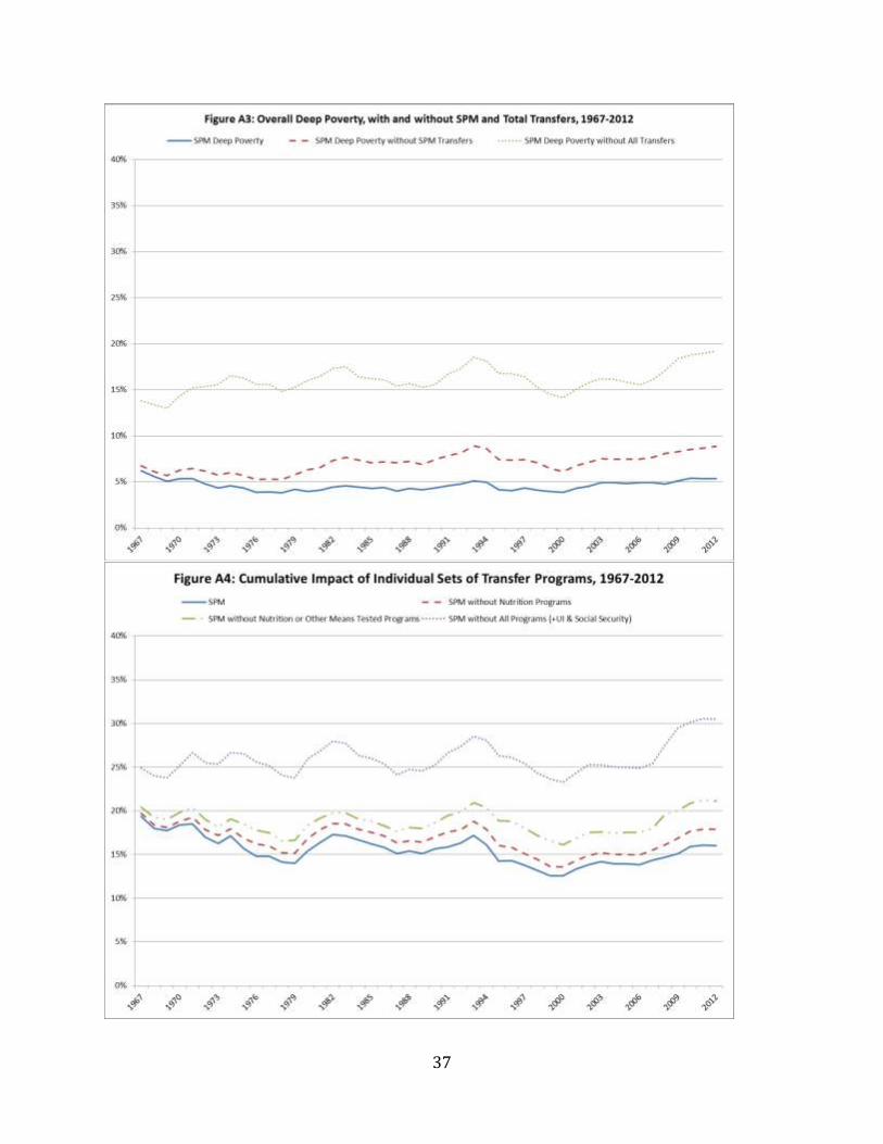
Figures 4a and 4b show the enormous difference transfer payments make in reducing both

poverty and deep poverty rates. For instance, in 2012, we estimate the deep poverty rate (the

share of the population with income below 50 percent of the poverty threshold) under the SPM to

be only 5.3 percent, while if no transfers were included, the deep poverty rate would be 19.2

percent – over 3 times higher. Similarly, the poverty rate (the share of the population with

income below the poverty threshold) is roughly 16 percent under the SPM in 2012, but absent

government transfers, would be about 31 percent -- nearly double.

The second striking finding that emerges from Figures 4a and 4b is the extent to which

government transfers seem to mute the effects of the business cycle, especially for deep poverty.

In Figure 4b, we can see how – without government transfers -- the poverty and deep poverty

rates would have climbed and fallen during and after the early 1980s recessions, the early 1990s

recession, the early 2000s recession, and most recently the Great Recession. Contrast that with

14 In a detailed and exhaustive study of means-tested and social insurance programs in the U.S., Ben-Shalom,

Moffitt, and Scholz (2011) document that while many programs have behavioral effects, their aggregate effect is

tiny and does not affect the magnitude of their anti-poverty impact. Earlier studies based on historical data have

reached similar conclusions (see Danziger, Haveman, and Plotnick, 1981; Moffitt, 1992 for a review of the earlier

literature). 15

While Child Tax Credits are included in our overall federal tax estimates, we are not able to consistently break out

the CTC in the CPS in years after it was adopted in 1997, as this is not one of the tax variables the Census includes

on public use files between 1997-2004 (it is included from 2005 onwards). Other refundable tax credits are similarly

not available prior to 2005, meaning the counterfactual series above likely understates the full role of transfers in

reducing poverty rates. 16 Government pensions are only included in the series from 1967-1974. After that they are not separately identifiable from other retirement income in the CPS.

12

the deep poverty rate trend in Figure 4a, which takes the full array of transfers into account,

where deep poverty never rises above 6.2 percent, and generally hovers between 4 and 6 percent.

This buffering effect is somewhat less evident in the overall poverty rate, but even here the rise

and fall in poverty rates across the business cycle is less dramatic after including transfers than

before.

We next examine the impact of transfer programs on child poverty. In Figure 5a, we show child

poverty rates under the SPM and then – in the counterfactual scenarios – under the SPM but

without key government transfers. Again we show what poverty rates would be in the absence of

all transfer programs, but here we also show the distinct effect of the transfer programs newly

counted under the SPM. We do this because many of these programs (SNAP/Food Stamps,

EITC, WIC, School Meals) are explicitly targeted at families with children or are of much more

monetary value for families with children than for other households.

As shown in Figure 5a, including the SPM transfers in the poverty measure makes a substantial,

and growing, difference in estimating child poverty rates. Absent the programs newly counted

under the SPM, child poverty rates would be over 8.5 percentage points higher in 2012 – 27.3

percent vs. 18.8 percent. And absent all government programs, child poverty would be nearly 12

percentage points higher in 2012 – 30.6 percent vs. 18.8 percent. In both cases, these impacts on

poverty rates have grown over time. For example, all transfers reduced child poverty rates by just

under 3.5 percentage points in 1967, but this anti-poverty effect grew steadily to about 8

percentage points in 1970s and early 1980s. Prior to the Great Recession, the impact of transfers

on child poverty peaked at about 10 percentage points in the mid-1990s before reaching record

highs in the past few years. Likewise, the impact of the package of transfers newly counted in the

SPM has steadily increased over time, from just under 1 percentage point in 1967 to nearly 9

percentage points in the past few years.

Figure 5b provides the same estimates for the total population. It again illustrates the role played

by government programs in reducing poverty.

Figures 6a and b illustrate this more directly by showing what the poverty rate would be for the

total population with and without government transfers in selected years (Figure 6a) and the

percentage point reduction in poverty documented in SPM vs. OPM (Figure 6b). These figures

indicate that the role of government transfers has grown from reducing poverty by under 6

percentage points in 1967 to nearly 15 percentage points in 2012. OPM estimates would capture

most of this in 1967 (5 out of 6 percentage points) but would capture a lesser portion in 2012 (9

out of 15 percentage points). This is because most government transfers were cash-based in the

1960s, and thus captured in the OPM. But today in-kind and post-tax transfers have grown much

more important, and their role would be missed in the OPM, where they are simply not counted

in families’ resources.

Figure 7 shows the effect of government transfers for deep child poverty rates (the share of

children with incomes below 50 percent of the poverty threshold).17

As with the pictures for the

total population in Figures 4a and b, it is remarkable how flat the SPM deep poverty rate for

children is relative to what deep poverty rates would have looked like absent accounting for

17

Appendix Figure A3 provides the same estimates for the total population.

13

safety net transfers. Figure 7 demonstrates how transfers help protect children from the

consequences of the business cycle, keeping deep poverty relatively low and steady in the face of

changes in the wider economy. In 2012, deep poverty would be nearly 11 percentage points

higher for children – 16.4 percent vs. 5.4 percent – absent government transfers.

The analysis thus far has added together the many types of transfer programs that government

provides. In Figure 8, we look at different types of programs and the role each plays in reducing

child poverty rates. We consider three particular types of support: food and nutrition programs

(SNAP/Food Stamps, School Lunch, WIC); other means tested programs (SSI, TANF/AFDC,

housing subsidies, EITC, and LIHEAP); and social insurance programs (primarily Social

Security and Unemployment Insurance, but also smaller programs like Worker’s Compensation

benefits, Veteran’s payments, and other government pensions).18

The impact of the food and nutrition programs is very small at the start of our time series, as

SNAP/Food Stamps were still only available to a very small percentage of the population, WIC

was not yet created, and the School Lunch Program provides small benefit values that are

unlikely to lift many people above the poverty line. But the importance of the food and nutrition

programs grows markedly over time following the national spread of SNAP (then called Food

Stamps) in the 1970s. The impact of food and nutrition programs is the largest in the last few

years, together reducing child poverty rates by approximately 3-4 percentage points.

When we add in other means-tested programs, the percentage point reduction in poverty rates

typically jumps quite a bit, and stands at about 9 percentage points in the modern period, which

was rivaled only in the mid-1990s prior to welfare reform, when the EITC had been expanded

but cash welfare had not yet been reformed (see more on this below). We see a bit more

reduction in child poverty rates when we add in the social insurance programs. In the early

period these programs jointly (along with food/nutrition and other means-tested programs)

reduced child poverty rates by only 3-4 percentage points. Today these transfer programs taken

together reduce child poverty rates by nearly 12 percentage points, demonstrating the growing

importance of transfer programs in keeping the poverty rate down. It is worth noting that when

quantified as the percentage point reduction in the child poverty rate, the impacts of all three

types of transfers system were at an all-time high between 2009-2012.

The Growing Importance of Tax Credits

One of the motivating forces behind the creation of the SPM was that the OPM does not count

after-tax income. Tax credits as an anti-poverty program became increasingly important for

many low-income families after the expansions of the EITC in the early 1990s. At the same time,

cash welfare – which is captured in the OPM – began to play a less important role, as federal

welfare reform in 1996 time-limited the program and added work requirements, subsequent to

which caseloads dropped precipitously.

In Figure 9, we juxtapose trends in the SPM poverty rate absent cash welfare benefits and absent

the EITC relative to the actual SPM poverty rate. We focus here on child poverty, as both

programs are largely targeted at families with children.

18

Appendix Figure A4 provides the same estimate for the total population

14

Three things become evident from Figure 9. First, cash welfare used to play a substantial role in

reducing child poverty in America. In the 1970s and 1980s, for instance, the AFDC program

reduced estimated child poverty rates by approximately 2 percentage points. But after 1996,

welfare’s impact on poverty rates dissipates very quickly, to the point where in the current period

the program reduces child poverty rates by only about one half of a percentage point. Second,

Figure 9 shows how the EITC has become increasingly important as an anti-poverty program, in

a fashion that is essentially the mirror image of the disappearance of cash welfare.19

When the

program was established in 1975, its effects on child poverty rates were minimal (as the benefit

was quite small). This pattern persisted until the major expansions to the EITC in the mid-1990s.

Since then, its impact on child poverty rates has grown steadily, topping out at nearly five

percentage points in the current period. Third, the anti-poverty impact of the EITC at its

maximum (4.8 percentage points in 2012) is larger than the impact of cash welfare at its

maximum (2.7 percentage points in 1991).20

The role of the EITC as a key anti-poverty policy in recent decades can also be contrasted with

the role the tax system played in earlier decades. Figure 10 shows what child poverty rates would

be with and without taking taxes and tax credits into account. It shows that until the expansions

of the EITC in the mid-1990s, the tax system acted to increase poverty. In contrast, since the

expansion of the EITC, the tax system as a whole has been poverty-reducing, reflecting the

important role played by EITC (and, to a lesser extent, the CTC).

Conclusion

As we near the 50th

anniversary of the War on Poverty, the overall poverty rate – at first glance --

appears to be much the same today as it was back then. Under the OPM, overall poverty was 14

percent in 1967 and 15 percent in 2012. Even under the improved SPM, overall poverty is not

much lower today than it was back then – down from 19 percent to 16 percent. Does this mean

that the War on Poverty has had little or no effect on poverty? To answer this question, we need

to know the counterfactual – what poverty rates would be today in the absence of government

19

The role of tax credits would be even larger if we were able to include the CTC alongside the EITC in our

estimates. 20

Figure 9 considers the impact of government programs on moving children above the poverty threshold, but not

their potential impact on reducing deep poverty among children below the poverty threshold. Cash welfare

programs, targeted at very low-income families, may do more to reduce deep poverty than overall poverty.

Appendix Figure A5 provides evidence on this point, displaying the same type of estimates, but focusing on deep

child poverty. Like Figure 9, Appendix Figure A5 shows the declining importance of cash welfare, and the growing

importance of the EITC. But in contrast to Figure 9, we see much larger impacts of the TANF/AFDC program at its

peak (reducing deep child poverty rates by 5.3 percentage points in 1983-84) than the EITC at its peak (reducing

deep child poverty rates by 1.7 percentage points in 2002). On the surface it may appear that the move from cash

welfare to a more employment-focused anti-poverty strategy involved a tradeoff between combating deep poverty at

the very bottom of the income distribution to aiding people who are closer to the poverty line to begin with. It is

worth noting, however, that deep poverty rates for children have stayed fairly low and flat, suggesting that other

aspects of anti-poverty policies, like an expanded and more robust SNAP/Food Stamps program, likely made up for

some of the impact that cash welfare lost in lowering deep poverty rates. Finally, as documented in other research,

behavioral changes (e.g., increases in employment in response to a more employment-focused anti-poverty system)

also helped neutralize the effect of lost cash welfare income on poverty (Blank, 2002; Kaushal and Kaestner, 2001).

15

anti-poverty programs. Producing this counterfactual is challenging, since it would require

estimating behavioral models of how individuals and families would respond if government

programs did not exist. In this paper, we have a more modest goal – to provide an accounting of

the poverty rates that would exist if we did not take into account the full range of benefits

families receive from government programs.

Our analysis has four main findings.

First, we find that historical trends in poverty have been more favorable -- and that government

programs have played a larger role -- than OPM estimates suggest. The OPM shows the overall

poverty rates to be nearly the same in 1967 and 2012 – at 14 and 15 percent respectively. But our

counterfactual estimates using SPM show that without government programs, poverty would

have risen from 25 percent to 31 percent, while with government benefits poverty has fallen from

19 percent to 16 percent. Thus government programs today are cutting poverty nearly in half

(from 31 percent to 16 percent) while in 1967 they cut poverty by only a quarter (from 25

percent to 19 percent).

Second, government programs play a substantial and growing role in alleviating child poverty,

and particularly deep child poverty -- a role that would be masked in estimates using the OPM.

Taken together, government programs in 2012 reduced child poverty by 12 percentage points,

and deep child poverty by 11 percentage points, vs. 3 and 5 percentage points respectively in

1967. Estimates from OPM would miss much of this poverty reduction, particularly in the

modern period when cash welfare plays a smaller role.

Third, the impact of government anti-poverty programs is particularly pronounced during

economic downturns – so these programs play an important role in protecting individuals and

families from the vagaries of the economic cycle. Without government programs, deep child

poverty rates would be as high as 20 percent during economic downturns, as opposed to the 4-6

percent rates we observe with government programs. Again, this role is missed in OPM

estimates.

Finally, by using a measure that takes into account the full array of government anti-poverty

programs, we are able to quantify the impact that different types of programs play. Our estimates

point to a particularly crucial role for tax credits and food and nutrition programs, especially in

the modern era. In 2012, the EITC and food and nutrition programs reduced child poverty rates

by approximately 5 and 4 percentage points respectively, up from less than 1 percentage points

each in 1967. Again, this impact would be missed by OPM, which does not count the value of

either set of programs.

Although our estimates are informative, much remains to be done. As mentioned, we hope to

augment the data presented here with data from 1959, prior to the War on Poverty. In addition,

an important issue not addressed in our work here is the problem of under-reporting of benefits

in the March CPS; to the extent that benefits are under-reported, and such under-reporting has

grown over time (Wheaton, 2008), this will lead us to under-estimate the role played by

government policies, and more so over time. Meyer and Sullivan (2012a, b) argue that such

under-reporting is one reason why consumption-based estimates show more reduction in poverty

16

over time than do income-based ones. And, as discussed, the inclusion of MOOP in the SPM is

controversial (see e.g., Korenman and Remler, 2012; Meyer and Sullivan, 2012). We would like

to experiment with alternative ways to take medical expenses into account.

Finally, it is useful to recall that both the OPM and SPM are income-based poverty measures and

as such capture only one dimension of disadvantage. There continues to be a need for further

development and research on measures that capture income poverty alongside disadvantage in

terms of other dimensions such as wealth, material hardship and well-being (Wimer et al.,

2013b).

17

References

Ben-Shalom, Yonatan, Robert Moffitt, and John Karl Scholz (2011). “An Assessment of the

Effectiveness of Anti-Poverty Programs in the United States.” Available from:

http://www.npc.umich.edu/publications/working_papers/

Betson, David, and Robert Michael. (1993) "A Recommendation for the Construction of

Equivalence Scales." Unpublished memorandum prepared for the Panel on Poverty and

Family Assistance, Committee on National Statistics, National Research Council.

Department of Economics, University of Notre Dame.

Bitler, Marianne and Hilary Hoynes (2013). “The More Things Change, the More They Stay the

Same: The Safety Net, Living Arrangements, and Poverty in the Great Recession.” Paper

presented at the NBER Conference on Labor Markets after the Great Recession.

Blank, Rebecca (2002). “Evaluating Welfare Reform in the United States.” Journal of Economic

Literature, 40(4), 1–43.

Blank, Rebecca M. (2008). "Presidential address: How to improve poverty measurement in the

United States." Journal of Policy Analysis and Management 27.2, 233-254.

Blank, Rebecca and Mark Greenberg (2008). “Improving the Measurement of Poverty.” The

Hamilton Project, Discussion paper 2008-17.

Bohn, Sarah, Caroline Danielson, Matt Levin, Marybeth Mattingly, and Christopher Wimer

(2013). The California Poverty Measure: A New Look at the Social Safety Net. San

Francisco, CA: Public Policy Institute of California.

Cable, Dustin. (2013). “The Virginia Poverty Measure: An Alternative Poverty Measure for the

Commonwealth.” University of Virginia—Welden Cooper Center for Public Service,

Demographics and Workforce Group.

Casper, Cohen and Simons (1999). Documention. Available from:

http://www.census.gov/population/www/documentation/twps0036/twps0036.html

Citro, Constance and Robert Michael (eds.) (1995). Measuring Poverty: A New Approach.

Washington D.C.: National Academy Press, 1995.

Danziger, S., R. Haveman and R. Plotnick. 1981. “How Income Transfer Programs Affect Work,

Savings, and the Income Distribution: A Critical Review.” Journal of Economic

Literature 19 (September): 975-1028.

Engelhardt, Gary V., and Jonathan Gruber. (2006). “Social Security and the Evolution of Elderly

Poverty.” In Auerbach, Card, and Quigley (eds.) Public Policy And the Income

Distribution, 259-287. New York: Russell Sage.

18

Feenberg, Daniel, and Elisabeth Coutts (1993). “An Introduction to the TAXSIM Model.”

Journal of Policy Analysis and Management 12: 189-194.

Garner, Thesia (2010). “Supplemental Poverty Measure Thresholds: Laying the Foundation.”

Washington, DC: Bureau of Labor Statistics.

Hoynes, Hilary W. (2012). “Comment on Meyer and Sullivan.” Brookings Papers on Economic

Activity (Fall): 184-189.

Hutto, Nathan, Jane Waldfogel, Neeraj Kaushal, and Irv Garfinkel (2011). “Improving the

Measurement of Poverty.” Social Service Review 35(1): 39-74.

Iceland, John. (2005). "Measuring poverty: Theoretical and empirical considerations."

Measurement: Interdisciplinary Research and Perspectives 3(4), 199-235.

Johnson, Paul, Trudi Renwick, and Kathleen Short. “Estimating the Value of Federal Housing

Assistance for the Supplemental Poverty Measure.” Washington D.C.: U.S. Census

Bureau, Social, Economic, and Housing Statistics Division, 2010.

Levitan, Mark et al. (2010). "Using the American Community Survey to create a National

Academy of Sciences-Style Poverty Measure: Work by the New York City Center for

Economic Opportunity" Journal of Policy Analysis and Management 29(2): 373-386.

Kaushal, Neeraj, and Kaestner, Robert (2001). “From Welfare to Work: Has Welfare Reform

Worked?” Journal of Policy Analysis and Management 20(4): 740–761.

Korenman, Sanders and Dahlia Remler (2012). “Rethinking Elderly Poverty: Time for a Health

Inclusive Poverty Measure?” Oct. 19, 2012 draft presented at 2012 APPAM Meetings.

Meyer, Bruce D. and James X. Sullivan (2003). “Measuring the Well-Being of the Poor Using

Income and Consumption.” Journal of Human Resources 38(S): 1180-1220.

Meyer, Bruce D. and James X. Sullivan (2012a). “Five Decades of Consumption and Income

Poverty.” NBER Working Paper 14827.

Meyer, Bruce D. and James X. Sullivan (2012b). “Winning the War: Poverty from the Great

Society to the Great Recession.” Brookings Papers on Economic Activity (Fall): 133-183.

Meyer, Bruce D. and James X. Sullivan (2012c). “Identifying the Disadvantaged: Official

Poverty, Consumption Poverty, and the Supplemental Poverty Measure.” Journal of

Economic Perspectives 26(3): 111-136.

Meyer, Bruce D., and James X. Sullivan (2013). "Consumption and Income Inequality and the

Great Recession." American Economic Review 103(3): 178-83.

Moffitt, R. 1992. “Incentive Effects of the U.S. Welfare System: A Review.” Journal of

19

Economic Literature 30 (March): 1-61.

NYC Center for Economic Opportunity (2013). “The CEO Poverty Measure 2005-2011: An

Annual Report by the NYC Center for Economic Opportunity.” Available from

http://www.nyc.gov/html/ceo/downloads/pdf/ceo_poverty_measure_2005_2011.pdf

[accessed October 10, 2013).

Renwick, Trudi (2011). “Geographic Adjustments of Supplemental Poverty Measure Thresholds:

Using the American Community Survey Five-Year Data on Housing Costs,” SEHSD

Working Paper Number 2011-21, U.S. Census Bureau.

Short, Kathleen (2011). “The Research Supplemental Poverty Measure: 2010.” Current

Population Reports P60-241.

Short, Kathleen (2012). “The Research Supplemental Poverty Measure: 2011.” Current

Population Reports P60-244.

Short, Kathleen (2013). “The Research Supplemental Poverty Measure: 2012.” Current

Population Reports P60-247.

Smeeding, Timothy M. (1977). "The antipoverty effectiveness of in-kind transfers." Journal of

Human Resources, 360-378.

Smeeding, Timothy M., Julia B. Isaacs, and Katherine A. Thornton. 2013. “Wisconsin Poverty

Report: Is the Safety Net Still Protecting Families from Poverty in 2011?” University of

Wisconsin-Madison Institute for Research on Poverty.

Wheaton, Laura. "Underreporting of Means-Tested Transfer Programs in the CPS and SIPP."

(2008). Washington, DC: The Urban Institute.

Wheaton, Laura, Linda Giannarelli, Michael Martinez-Schiferl and Sheila Zedlewski. 2011.

“How Do States’ Safety Net Policies Affect Poverty?” Working Families Paper 19, Urban

Institute.

Wimer, Christopher, Liana Fox, Irwin Garfinkel, Neeraj Kaushal, Jane Waldfogel, and

Christopher Wimer (2013a). “Trends in Poverty with an Anchored Supplemental Poverty

Measure.” Columbia Population Research Center Working Paper.

Wimer, Christopher, Irv Garfinkel, Madeleine Gelblum, Narayani Lasala Blanco, Yajuan Si,

Julien Teitler, and Jane Waldfogel (2013b). “Income Poverty and Material Hardship in

New York City: Evidence from a New Household Survey.” Presented at the Population

Association of America Annual Meeting, May 2013.

20

21

22

23

24

25

26

27

28

Technical Appendix

This appendix provides more detail about the methods used to construct our historical SPM

series.

Poverty Units

Unmarried partners are directly identified in the CPS since 1995, so for years prior to that we

must seek to identify them through other means. We use the well-established adjusted-POSSLQ

routine (which stands for Persons of the Opposite Sex Sharing Living Quarters). We follow

Casper, Cohen and Simmons (1999), who define an adjusted POSSLQ household as one that

meets the following criteria: two unrelated adults (age 15+) of the opposite sex living together,

with no other adults except relatives and foster children of the reference person, or children of

unrelated subfamilies.

Prior to 1988, it is not possible to identify foster children in the CPS (and instead they are coded

as unrelated individuals), so foster children between the age of 15-22 are excluded from SPM

family units from 1967-1987.

From 2007 onwards, detailed relationship codes make it possible to identify and include both

biological parents of a child in a household even if these individuals do not claim to be

unmarried partners. However, prior to 2007, these detailed relationship codes are not available,

so we must rely on relationship codes of individuals in reference to household head or family

reference person. Prior to 1975, only relationship to household head exists, not relationship to

family head.

Equivalence Scale

We follow the Census Bureau in using a three-parameter equivalence scale to adjust poverty

thresholds for poverty-unit size and composition. This equivalence scale is as follows:

Families without children:

Equivalence scale=(adults)0.5

Single parents:

Equivalence scale=(adults+0.8*first child+0.5*other children)0.7

All other families:

Equivalence scale=(adults+0.5* children)0.7

Geographic Adjustment

The SPM adjusts poverty thresholds for geographic differences in the cost of housing.

Specifically, they use five-year American Community Survey data on rental payments in

metropolitan areas to adjust the shelter and utilities component of the SPM poverty thresholds. In

contrast, our historical-SPM estimates do not yet adjust poverty thresholds for geographic

differences in cost-of-living given the paucity of consistent data back to 1967 necessary to

implement geographic adjustments. Developing a method of implementing a consistent

29

geographic adjustment over time remains an important area for future research. For more on

geographic adjustment under the SPM, see Renwick (2011).

Mortgage Status

Data for constructing thresholds by housing status are not consistently available for all years.

From 1976-2008, the CPS asks respondents whether they owned or rented their dwelling, but not

about their mortgage status, a question has been included since 2009. There are no housing

tenure questions in the CPS prior to 1976.

To follow the Census SPM methodology, which require thresholds based on three housing status

groups, we imputed mortgage status from the CEX to the CPS in 1980-2009 and in 1972/73.

This imputation included poverty status, age, race, education and marital status of household

head, family size and region as well as race*education interactions and race*age interactions. For

the intermediate years 1974-1979 the coefficients were linearly interpolated and applied to CPS

data to estimate predicted likelihoods of having a mortgage among home owners. For 1967-

1971, the same annual rate of change in the relationships between 1972/3-1980 was assumed and

extrapolated to the earlier years.

Prior to 1974, a two-step imputation process was applied, first to determine ownership vs renter

status and second to determine mortgage status among owners. The first imputation included the

same covariates as the mortgage status imputation described above but also included deciles of

income and welfare recipiency. The incidence rate of ownership was constrained to match the

incidence in the CEX.

SNAP

To impute SNAP benefits into the CPS for years prior to 1979, we first impute receipt of benefits

to household heads or primary individuals (which we jointly call “heads”). To accomplish this,

we first estimated the percent of heads in 1980 who reported receiving food stamps in 1979. We

then harnessed administrative data on caseloads published by the USDA. The USDA provides

annual caseloads (average monthly caseloads for a given year) for every year back to 1969. We

were able to add caseloads back to 1967 using data from the Statistical Abstract(s) of the United

States to create a consistent time series across the entire period. We then took the estimated

percent of heads receiving food stamps in 1979, and estimated the same percent for prior years

using rate of change in the caseload after adjusting for overall population growth. This estimated

percent of heads receiving food stamps then served effectively as the percentage of heads we

would constrain our imputation to. It should be noted that SNAP receipt is underreported in the

CPS, such that by taking the percentage of reported receipt in the 1980 CPS and deflating it

backwards historically using changes in the caseload, our imputation procedure produces

similarly underreported estimates of SNAP in earlier years, such that no break will appear in

trend lines starting when SNAP receipt is self-reported. This is also true for our other

imputations.

The basic method for deciding who to assign SNAP receipt to in a given year of the CPS was to

run a linear probability model within the 1972-1973 Consumer Expenditure Survey predicting

30

receipt of food stamps among consumer unit heads. The factors used to predict SNAP receipts

were receipt of public assistance/welfare, number of children, unemployment status, a dummy

for having one adult in the family, a dummy for having 3 or more adults in the family, age

categories, education categories, race, family size, a dummy for being married, and race x

education interaction terms. We then computed the predicted probability of receiving food

stamps from this model, and used the same covariates from that model in a given year of the CPS

to impute CPS heads’ probability of receiving food stamps. The constraint factor was then used

to determine the cutoff for assigning SNAP receipt. For example, if we estimated that 6 percent

of heads in the CPS should be receiving food stamps in a given year, we would assign the 6

percent of CPS heads with the highest predicted probability of receiving food stamps as the

group for whom we impute a benefit.

The next step in our imputation process is to actually assign a value to the food stamps received.

It is worth noting that in the 1970s, the Food Stamp Program still had a “purchase requirement,”

which depending on your income, would dictate how much a family would have to pay for, say,

$100 worth of food stamps. So the value of the benefit in the 1970s is the difference between the

total value of the benefit and the amount families are required to purchase that total value. This is

called the “bonus value,” and is the amount we attempted to impute to recipients. To accomplish

this, we used a hotdeck procedure based on poverty status, receipt of other public assistance,

number of children, and number of adults. We cross-classified these variables into 36 mutually

exclusive groups, and found ten deciles of bonus values within each group. We find the same

mutually exclusive groups in the CPS for a given year, and within these groups randomly assign

people to the decile values established for their group in the CEX. Since the CEX is from 1972-

73, we then updated estimated imputed values for inflation using the CPI-U. This estimated

benefit value was then assigned to everyone else in the heads’ SPM unit. To bring values up

from 1972-73 to, say, 1976, we inflate the imputed values by the ratio of the average benefit

level in 1976 to the average benefit level in 1972-73 (an average of those two years’ average

benefit levels).

School Lunch Program

Our approach for imputing participation in the school lunch program is largely similar to our

imputation of SNAP, and included the same set of predictors. Because no information exists on

this program in the 1972-73 CEX, however, our dataset used for imputation is the 1980 CPS. As

with SNAP, we constrain the percentage of heads down (or up) each preceding year scaled by

changes in the administrative caseload. The administrative data here comes from the USDA and

was compiled back to 1969 by Robert Moffitt and his colleagues. We extended the series back to

1955 using information from the Statistical Abstracts of the United States. To assign monetary

values to those for whom we impute benefit receipt, we use the same model but predicting the

1980/79 family value of school lunch calculated by the Census. We then deflate this benefit by

the CPI-U.

WIC

Our procedure for imputing WIC benefits into the CPS is a two-step procedure. First, for years

prior to 2001, we imputed WIC incidence at the household level. Second, we calculate the

31

benefit value for all years using administrative data on average per person WIC expenditures

(see: http://www.fns.usda.gov/pd/wisummary.htm).

WIC Incidence: From 2001 onwards, the number of WIC recipients per household was reported

in the CPS. However, as nearly all families (>95 percent) who reported receiving WIC, only

reported receiving it for a single family member, we only impute a yes/no incidence instead of

the number of recipients per household. To estimate incidence, we first identified all families

currently automatically income-eligible for WIC: those currently receiving food stamps, public

assistance or Medicaid, with at least one child age 5 or below. While WIC is also available for

pregnant women without children, we have no way of identifying pregnant women in the CPS.

WIC also has a nutrition risk requirement for eligibility based on medical/nutritional guidelines

that we cannot observe in the CPS, so some income eligible families would likely be

nutritionally ineligible, but we cannot distinguish between these families in the CPS.

To constrain the number of recipients, we first estimate the share of WIC income-eligible

families from the CPS to administrative participation data for 2001-2010 and then constrain the

number of recipients in earlier years to match this ratio. We use OLS regression to estimate the

likelihood of WIC receipt among income eligible families, based on number of eligible kids,

household income and poverty status. While WIC was permanently established in 1974, only a

small number (88,000) individuals participated. As a result, we do not believe we can accurately

identify recipients in this year and estimate WIC beginning in 1975.

WIC Value: We calculate WIC value by multiplying the average annual WIC food costs per

person (based on monthly USDA administrative costs*12 from

http://www.fns.usda.gov/pd/wisummary.htm) by the number of recipients per household (which

is 0-4 from 2001-2012 and 0-1 prior to 2001). This value is then divided evenly among

household members and summed for SPM family units.

Housing Assistance

Our imputation model for receiving housing assistance is largely similar to that for SNAP and

school lunch, though here we predict for renting heads. The administrative data are also

somewhat different. We begin with a time series produced by Robert Moffitt and colleagues and

taken from HUD data that shows total households receiving direct housing assistance

administered by HUD. This series, however, only exists back to 1977. So we take a second

series, total outlays for discretionary housing assistance, which we were able to extend back to

1962 (Moffitt’s tables go back to 1970). The source of the data is the same as Moffitt’s, White

House historical budget tables. When expressed in constant dollars and compared against the

total number of households receiving direct housing assistance, however, we find that the cost

per household rose substantially over time between 1977 and the present. This may be because

the universe of what is covered under all discretionary housing assistance is larger and changes

over time relative to the number of units assisted under low-income housing assistance programs

like public housing and Section 8. Nevertheless, this makes it difficult to know how best to “back

out” the number of households receiving assistance for years prior to 1977, which is the

administrative data series we would ideally want. The trend in “cost per household,” however,

between 1977 and the present (2009) was roughly linear, however. So we assume that this trend

32

would extend back in time between 1967 and 1977. So with the total dollars spent and our

estimate of the number of dollars per household, we are able to divide out and reach an estimate

of the total number of households assisted. We then use this to constrain the percentage of

households we assign subsidy receipt to from the imputation model.

The Census values housing assistance by taking the lesser of (a) the shelter portion of the

threshold minus estimated rental payments, or (b) the market value of the housing unit minus

estimated rental payments (for an extended discussion see Johnson et al., 2010). We lack

adequate data to fully estimate rental payments and market values of housing units back to 1967.

We therefore adopt a simpler approach. To estimate rental payments, we assume that people

spend 30 percent of their household income on rent. This is a simplification of more complex

HUD guidelines, but modeling the more complex HUD guidelines would require knowing more

information than is available in the CPS all the way back to 1967. We then estimate the value as

the shelter portion of the threshold minus these estimated rental payments. When this simpler

approach is executed in data where we have the actual SPM (2009 to 2012), we find that our

approach leads to an overestimate of the impact of housing subsidies on poverty rates. We

therefore examined the ratio of Census estimated housing subsidy values to our subsidy values in

each year and found them to be approximately 89 percent in all three years at the median. So we

applied a correction factor of .89 to our estimated housing subsidy valuation in all years. This

correction factor yielded much closer estimates of the impact of including housing subsidies on

poverty rates in 2009 to 2012. Improving the historical estimation of housing subsidy valuation

is an important area for future work.

Taxes

After-tax income is not available on the CPS files before 1979/80. So we used NBER’s Taxsim

Program to calculate our after-tax estimates for earlier years. The starting point for our tax

programs are Stata programs provided by NBER and created originally by Judith Scott-Clayton.

We modify these for earlier years as income components that can go into the tax calculator begin

falling off of the CPS or become combined with other categories of income in the CPS. We also

made the simplifying assumption of using $0 versus positive income in the determination of

filing status (as compared to legal filing requirements) as we were not able to locate historical

data on tax filing requirements. Since such data surely exists, this is an important area for

potential improvement in our tax models in the future. We observed no major deviation in the

distribution of our after tax income variables, however, between 1978 and 1979

NBER’s Taxsim program only calculates state tax rates back to 1978. Prior to 1978, we

estimated family state income tax liability after credits by multiplying the median share of state

to federal tax liability for each state by each family’s estimated federal tax liability. Prior to

1976, not all individual states are identifiable in the CPS and instead regional groupings or

combinations of several states are provided. In these cases, we used the median tax rate for

families in the combined region.

33

MOOP

Medical out-of-pocket expenses (MOOP) are imputed from the CEX to the CPS for all years. We

use a hot-deck imputation strategy to calculate deciles of MOOP expenditures for consumer units

in the CEX for 10 imputation groups, based on: number of elderly in family (0,1,2), an indicator

for families of 1, and poverty level (below 200% and >=200% FPL). The distribution of MOOP

expenditures in each imputation group is preserved by randomly assigning deciles of

expenditures to the same imputation groups in the CPS. Finally, total MOOP expenditures are

then capped at $6,700/person (adjusted to nominal dollars using CPI-U), which is the 2011

Medicare Advantage Part D non-premium cap, per recommendations in Korenman and Remler

(2012). This method indirectly imputes incidence for various demographic groups since deciles

of $0 in expenditures would remain in both datasets, but it does not force an exact percentage.

For 2011, the first year of overlap between MOOP expenditures asked in CPS and our imputed

measure, our imputed estimate of MOOP estimates the overall median expenditures and the

distribution fairly well, with some underestimation at the 95th

and 99th

percentiles of

expenditures (see Table A1 below). However, using our capped, imputed MOOP measure as

opposed to the CPS measure has a relatively minor impact on overall SPM poverty rates. A more

comprehensive imputation measure would include health insurance status, but unfortunately that

is not available in the CEX (unless premiums were paid for by the consumer unit).

We use the same CEX sample as we do for poverty thresholds (see above), which is a five-year

moving sample from 1984-2012 with progressively fewer years of CEX data back to 1980, and

then single-year estimates of MOOP expenditures for 1972/73 and 1980. For the intermediate

years 1974-1979 the decile expenditures were linearly interpolated. For 1967-1971, the same

annual rate of change in the expenditures between 1972/3-1980 was assumed and extrapolated to

the earlier years.

34

Table A1: MOOP Distribution, 2011 CPS

Overall

Families with 0 elderly

Actual from CPS

Capped Imputation Diff

Actual from CPS

Capped Imputation Diff

1% 0 0 0

0 0 0 5% 0 0 0

0 0 0

10% 0 0 0

50 0 -50 25% 486 486 0

400 215 -185

Mean 3,437 3,142 -295

3,544 2,688 -856 50% 2,277 2,277 0

1,835 1,600 -235

75% 5,104 4,976 -128

4,750 4,005 -745 90% 8,316 7,979 -337

8,700 7,979 -721

95% 14,110 11,071 -

3,039

12,168 11,071 -1,097

99% 17,224 13,400 -

3,824

22,180 11,071 -11,109

Families with 1 elderly

Families with 2+ elderly

Actual from CPS

Capped Imputation Diff

Actual from CPS

Capped Imputation Diff

1% 0 0 0

0 1,025 1,025 5% 100 1,117 1,017

1,157 2,314 1,157

10% 480 1,158 678

2,314 2,360 46 25% 1,357 1,616 260

3,187 4,120 933

Mean 4,153 3,870 -282

7,250 6,932 -318 50% 2,803 2,995 192

5,733 5,984 251

75% 5,260 5,225 -35

9,194 9,836 642

90% 8,934 7,814 -

1,119

13,414 13,400 -14

95% 12,237 10,937 -

1,299

16,514 13,400 -3,114

99% 22,287 14,413 -

7,874

27,897 18,183 -9,714

35

Child Care/Work Expenses

Child care expenditures are imputed from the CEX to the CPS for all years. We utilize a two-step

procedure to estimate child care expenditures. We first use the CEX to predict the likelihood of

using paid child care using the following covariates: number of children (1, 2, 3+), number of

adults in household (1, 2, 3+), poverty dummies (<100%, 100-200% and >200% FPL), head age

(<25, 25-34, 35-44, 45-54, 55-64, 65+), race (white, black, other), education of head (LTHS, HS,

SC, BA+), family size, married, race*education interactions, race*age interaction, and a region

indicator (Northeast, Midwest, South, West). We then apply these regression coefficients to the

relevant CPS year and predict the likelihood of paid child care for each household. We constrain

paid child care incidence in the CPS to match paid child care incidence in the CEX by number of

adults present in the household (1, 2, 3+).

After incidence is determined, we used a hot-deck imputation strategy to assign deciles of child

care expenditures to heads in the CPS based on: poverty level (<100%, 100-200% and >200%

FPL), # of children (1, 2 and >=3) and family status (married, unmarried, 3+ adults). We use the

same CEX sample and interpolation strategy as we do in the MOOP estimates (see above).

Work Expenses

Work expenses (e.g., commuting costs, uniform purchases, etc) are estimated based on an

analysis of the Survey of Income and Program Participation (SIPP) provided to us by the Census

Bureau. Using the SIPP, they estimate a median weekly value of work expenses from 1997 to

2012. We fix this value historically adjusting for CPI-U. Total work expenses for the consumer

unit are then calculated as 85 percent of median work expense multiplied by the number of

weeks worked, and summed for all workers above age 17 in the unit as per NAS panel

recommendations.

Child care expenditures and work expenses are combined and then capped so that their total does

not exceed the reported earnings of the lowest earning spouse/partner in the family

36

Appendix Figures

37

38