WASHINGTON UNIVERSITY SEVER INSTITUTE OF TECHNOLOGY DEPARTMENT OF COMPUTER SCIENCE AND ENGINEERING DESIGN OF ROUTERS FOR OPTICAL BURST SWITCHED NETWORKS by Jeyashankher Ramamirtham Prepared under the direction of Professor J. Turner A dissertation presented to the Sever Institute of Washington University in partial fulfillment of the requirements for the degree of Doctor of Science August, 2004 Saint Louis, Missouri
Transcript
WASHINGTON UNIVERSITY
SEVER INSTITUTE OF TECHNOLOGY
DEPARTMENT OF COMPUTER SCIENCE AND ENGINEERING
DESIGN OF ROUTERS FOR
OPTICAL BURST SWITCHED NETWORKS
by
Jeyashankher Ramamirtham
Prepared under the direction of Professor J. Turner
A dissertation presented to the Sever Institute of
Washington University in partial fulfillment
of the requirements for the degree of
Doctor of Science
August, 2004
Saint Louis, Missouri
WASHINGTON UNIVERSITY
SEVER INSTITUTE OF TECHNOLOGY
DEPARTMENT OF COMPUTER SCIENCE AND ENGINEERING
ABSTRACT
DESIGN OF ROUTERS FOR
OPTICAL BURST SWITCHED NETWORKS
by Jeyashankher Ramamirtham
ADVISOR: Professor J. Turner
August, 2004
Saint Louis, Missouri
Optical Burst Switching (OBS) is an experimental network technology that
enables the construction of very high capacity routers using optical data paths and
electronic control. In this dissertation, we study the design of network components
that are needed to build an OBS network. Specifically, we study the design of the
switches that form the optical data path through the network.
An OBS network that switches data across wavelength channels requires wave-
length converting switches to construct an OBS router. We study one particular
design of wavelength converting switches that uses tunable lasers and wavelength
grating routers. This design is interesting because wavelength grating routers are
passive devices and are much less complex and hence less expensive than optical
crossbars. We show how the routing problem for these switches can be formulated as
a combinatorial puzzle or game, in which the design of the game board determines
key performance characteristics of the switch. In this disertation, we use this formu-
lation to facilitate the design of switches and associated routing strategies with good
performance.
We then introduce time sliced optical burst switching (TSOBS), a variant of
OBS that switches data in the time domain rather that the wavelength domain. This
eliminates the need for wavelength converters, the largest single cost component of
systems that switch in the wavelength domain. We study the performance of TSOBS
networks and discuss various design issues. One of the main components that is
needed to build a TSOBS router is an optical time slot interchanger (OTSI). We
explore various design options for OTSIs.
Finally, we discuss the issues involved in the design of network interfaces that
transmit the data from hosts that use legacy protocols into a TSOBS network. Ag-
gregation and load balancing are the main issues that determine the performance of
a TSOBS network and we develop and evaluate methods for both.
the optical components needed are expensive making it difficult for optical burst
switching to be an economically effective alternative to electronic networks. Most of
the optical packet switching studies have been done in research laboratories and have
not been successful in demonstrating a case for implementing optical packet switched
networks commercially.
Now we present a brief description of the architecture of an optical burst
switched network and present a summary of existing approaches for building opti-
cal switches.
1.1 Optical Burst Switching Concept
Optical Burst Switching (OBS) [7, 18, 78, 80, 79, 85, 91, 92, 95, 98, 101] is an experi-
mental network technology that seeks to use optical switching for the data path, while
still retaining the flexibility of electronics for control. By exploiting the high chan-
nel counts of advanced WDM systems, it achieves excellent statistical multiplexing
performance with little or no buffering.
The basic burst switching concept is illustrated in Fig. 1.1. The transmission
links carry data on tens or hundreds of wavelength channels and user data bursts
can be dynamically assigned to any of these channels by the OBS routers. One
(or possibly several) channel on each link is reserved for control information that
3
Burst Header Cell
Data Burst
Control Channel
Figure 1.1: Burst Switching Concept
is used to control the dynamic assignment of the remaining channels to user data
bursts. Terminals and/or other networks connect to a burst-switched network through
concentrators that convert data on lower speed interfaces (e.g. IP-over-Ethernet at
100 Mb/s or 1 Gb/s), to the burst data format. Concentrators may switch packets
received on low speed interfaces as single bursts, or may aggregate packets to form
larger bursts. Aggregation increases the average burst length on the links, potentially
improving efficiency and reducing the amount of control processing required. When a
concentrator has a burst of data to send, an idle channel on the access link is selected
and the data burst is sent on that channel.
Shortly before the burst transmission begins, a Burst Header Cell (BHC) is sent
on the control channel, specifying the channel on which the burst is being transmitted
and the destination of the burst. The OBS router, on receiving the BHC, assigns the
incoming burst to an idle available channel on the outgoing link leading toward the
desired destination and establishes a path between the specified channel on the access
link and the channel selected to carry the burst. It also forwards the BHC on the
control channel of the selected link, after modifying the cell to specify the channel on
which the burst is being forwarded. This process is repeated at every router along
the path to the destination. The BHC also includes an Offset field which contains
the time between the transmission of the first bit of the BHC and the first bit of
the burst, and a Length field specifying the time duration of the burst. The offset
and length fields are used to perform time switching operations in the OBS routers,
and the offset field is adjusted by the routers to reflect variations in the processing
4
delays encountered in the routers’ control subsystems. If a router does not have idle
channels available at the output port, the burst can be stored in a buffer.
Reference [91] describes a scalable OBS router architecture consisting of a set
of Input/Output Modules (IOM) that interface to external links and a multistage in-
terconnection network of Burst Switch Elements (BSE). The interconnection network
uses a Benes topology, which provides parallel paths between any input and output
port. A three stage configuration comprising d port switch elements can support
up to d2 external links (each carrying many WDM channels). The topology can be
extended to 5,7 or more stages. In general, a 2k − 1 stage configuration can support
up to dk ports. For example, a 5 stage network constructed from 8 port BSEs would
support 512 ports. If each port carried 256 channels at 10 Gb/s each, the aggregate
system capacity would be 1, 310 Tb/s.
Input IOMs process the arriving BHCs, performing routing lookups and in-
serting the number of the output IOM into BHCs before passing them on. The BSEs
use the output port number to switch the burst through to the proper output. Each
of the components that does electronic processing on the cell keeps track of the time
spent and updates the offset field in the BHC to maintain synchronization with the
burst.
The focus of the first part of this dissertation is the design of the optical data
path in each BSE. Optical components are used to build the BSEs and they are
electronically controlled by the switch controller to switch the data to the destination
output port, as determined by the route lookup in the IOM. We now present a brief
summary of the available optical technologies that can be employed to build such a
switch.
1.2 Enabling technologies
A typical optical switch has to implement three basic functions: demultiplexing and
multiplexing, switching, and contention resolution. The generic structure of an optical
packet switch is shown in Fig. 1.2. Demultiplexing of the individual wavelengths from
input fibers and multiplexing them back onto outgoing fibers is done using passive
couplers that are quite inexpensive. Switching is performed using high speed switching
components that are discussed later in this section. In a packet switch, contention
occurs whenever two or more packets try to leave the switch fabric on the same
output port at the same time. In electronic switches, contention resolution is handled
5
WDM fibers
Con
tent
ion
reso
lutio
n
Switching
Figure 1.2: Optical switch architecture
by using buffers and storing the packet that loses out on contention and transmitting
it at a later time when the outgoing channel becomes available. Typically, electronic
routers use buffers that can buffer about one half seconds worth of data or 5 Gigabits
for a 10 Gbps channel. The contention resolution can be done either at the input side
(before the switching) or at the output side (after the switching) or both.
There are three methods of contention resolution in optical systems, optical
buffering, wavelength conversion, and deflection routing. We now present an overview
of the technologies that are available to perform each of these functions [74, 84, 90].
1.2.1 Switching
Switching is the process of directing signals from an input port to an output port
as determined by the address lookup performed on the burst header cell. Optical
switches are available for a range of applications. Wavelength routed networks that
provision connections on a per-wavelength basis require switches with switching times
of the order of a millisecond. Packet switching or burst switching, on the other hand,
requires high speed switches (usually crossbars) to switch packets or bursts onto
outgoing links. The switching speed of the crossbar determines the minimum size of
the bursts that can be switched and the lower the minimum size of bursts, the better
the statistical multiplexing performance of the network. A packet of size 100 bytes is
about 80 ns long on an optical fiber that has a bandwidth of 10 Gbps per wavelength.
If we were to handle bursts of the order of 100 bytes, we need optical crossbars that
have switching times of 1-10 ns.
Apart from the switching time, other important characteristics of switches are
extinction ratio, insertion loss, and crosstalk. These characteristics determine the
6
quality of the signal when it is switched through the devices. Higher loss character-
istics imply that the signal needs to be regenerated more often in the network, which
amounts to an increase in cost of the system. Extinction ratio is the ratio of the
output power of a switch in the “on” state (when the input is connected to some
output) to the output power in the “off” state (when the output is not connected to
any input). This ratio should be as high as possible. While mechanical switches have
extinction ratios of 40-50 dB, high-speed switches have extinction ratios of 10-25 dB.
Insertion loss is the fraction of the signal power lost as a result of placing the switch
in the data path and must be as small as possible. In a switch, even if an input is
connected to some output, it is possible that power from other inputs can be coupled
onto the signal at the output. The crosstalk of a switch is the ratio of the power at
an output from the desired input to the power from all other inputs.
The two technologies that have switching times of a nanosecond or less are
Electro-optic Lithium Niobate based switches and semiconductor optical amplifiers
based switches. Other technologies that are commonly found like Micro-Electro-
Mechanical Systems (MEMS) switches [76], Liquid Crystal switches, and Bubble-
based Waveguide switches have switching times of a millisecond or more and cannot
be used for burst switching. Lithium Niobate switches have very fast switching times
of less than 1 ns and allow for modest levels of integration. A 16×16 switch with
nanosecond switching times has been demonstrated [75]. However, they have a rela-
tively high insertion and polarization dependent loss.
Semiconductor optical amplifiers (SOAs) are promising components that can
be used to build fast switches. An SOA is used as an on-off switch and is controlled
by a bias voltage. When in the off state, the signal is absorbed by the device and in
the on state, the signal is amplified. This results in very large extinction ratios. SOA
gate switching has been demonstrated in [33, 34, 53]. Reference [53] discusses the
construction of a 4 × 4 switch matrix using SOA gates and Reference [34] discusses
the construction of an 8 × 8 switch matrix. However, these switches are expensive
components and challenges remain in integrating them into large-scale switching fab-
rics. Also, use of SOAs results in amplified spontaneous emission noise and this leads
to degradation of the signal quality.
Reference [69] tabulates properties of the different switching technologies avail-
able.
7
1.2.2 Fiber delay lines
In optical switching systems, the only practical method of buffering is to circulate the
optical signal through a fiber delay line for the amount of time required [58]. If we use
a single lengthy fiber to store the packets, the amount of fiber required is excessive
(half a second corresponds to 150, 000 km of fiber) and fiber delay lines are also not
random access. The other approach to using fiber delay lines is to use a smaller
length fiber and recirculate the signal through the fiber repeatedly until the required
amount of delay is achieved. This method results in excessive signal degradation that
makes it impractical to use. Also, this method requires the use of WDM to maintain
high buffer capacity. Thus, optical packet switching systems typically use very little
buffering if any at all and depend on other contention resolution methods for good
performance.
For small amounts of buffering, fiber delay lines can be packaged by wrapping
the fiber around a cylindrical ring. The cladding diameter of a single mode fiber is
usually 125µm and there is a layer of coating on top of the cladding which makes the
diameter 250µm. A spool of fiber [2] that has an outer diameter of 27 cm (a little less
than 11 inches) and a width of 18 cm (less than 7 inches) holds 50 km of fiber. The
fiber delay lines may have to be temperature controlled depending on the conditions
because temperature variations can cause the signal quality to degrade.
1.2.3 Deflection routing
Deflection routing [16, 43, 51, 57, 72] is another contention resolution method that
has been studied. This is a multiple-path routing technique where packets that lose
contention are routed to nodes other than their next-hop nodes and get routed to the
destination from there on. Deflection routing is also known as hot-potato routing.
Deflection routing could cause out-of-order delivery of packets at the destina-
tion requiring resequencing. Also, the effectiveness of this method depends heavily
on the network topology and the offered traffic pattern. Deflection routing works well
in highly regular networks like the Manhattan Street network or the shuffle-exchange
network since a deflection does not result in a large “detour”. Thus, using deflection
routing reduces the flexibility in designing the network. Deflection routing also re-
sults in an increased delay through the network as compared to a network that uses
buffers to resolve contention. Another issue with using deflection routing is that pack-
ets/bursts can be routed away from the destination endlessly. This behavior, called
8
livelock, can be avoided by dropping the packet after a fixed number of hops. We do
not study deflection routing as a contention resolution mechanism in this dissertation.
1.2.4 Wavelength conversion
Wavelength conversion offers effective contention resolution without relying on buffers
at a switching node. By using wavelength conversion, we can switch bursts onto dif-
ferent output wavelength channels. Reference [91] presents the statistical multiplex-
ing performance of a multiplexor that uses wavelength conversion with and without
buffering. Also, wavelength conversion does not rely on the network topology or of-
fered traffic intensities to provide acceptable performance and it is not cumbersome
to use as compared to fiber delay lines. This makes it an ideal choice for contention
resolution in optical burst switches. Wavelength conversion technologies are discussed
in [32, 25, 105]. Very broadly, there are four types of wavelength conversion mecha-
nisms, optoelectronic, optical gating, interferometric, and wave mixing.
The optoelectronic approach converts the optical signal back into electronic
form and then retransmits it using a laser tuned to a different wavelength. There
are three types of optoelectronic converters depending on the kind of regeneration
used. Using 1R regeneration, where the incoming signal is simply amplified, makes
the system transparent to the modulation format of the signal and the converter
can handle analog data also. A wavelength converter employing 2R regeneration
performs reshaping of the signal in addition to amplifying it. This operation can be
performed on digital data only and it introduces additional phase jitter into the signal.
A wavelength converter employing 3R regeneration performs retiming of the signal
in addition to amplifying and reshaping it. This operation completely regenerates
the signal. However, retiming is bit-rate specific and hence, the transparency of
the system is lost. The rate of operation of optoelectronic wavelength converters is
determined primarily by the electronic circuitry and hence, wavelength converters
employing this method encounter bandwidth limitations at very high speeds. Also,
the power consumption of optoelectronic converters is very high. Optoelectronic
wavelength converters operating at 2.5 Gbps have been reported in References [36].
Wavelength converters based on optical gating make use of a device that acts
as a gate modulated by the input optical signal and the input information is trans-
ferred to a probe signal that is on a different wavelength. The target wavelength
is isolated at the output using a filter. The main technique using this principle is
9
cross-gain modulation (XGM), using a nonlinear effect in a semiconductor optical
amplifier (SOA). This device can handle bit rates of 10 Gbps and is expected to be
able to handle 100 Gbps. Also, this method of wavelength conversion is polarization
independent, can handle a wide range of input wavelengths, and has reasonably high
conversion efficiency (ratio of the output power to the input power of the probe).
However, this method has several drawbacks too. The achievable extinction ratio is
small and the input signal power must be high. Also, the carrier density and the
refractive index in the SOA varies resulting in pulse distortion and phase variation.
As the carrier density varies with the input signal in an SOA, the phase of the
probe is modulated (This results in pulse distortions in the converters based on the
optical gating technique described above). The phase modulation can be converted
into intensity modulation using an interferometer such as a Mach-Zehnder Interferom-
eter (MZI). This approach is called cross-phase modulation (XPM). The advantage of
this approach is that the input signal power needed is much lesser than in the optical
gating approach and can be used with high input probe power. Also, wavelength con-
verters using this method can achieve better extinction ratios. Reference [70] reports
an implementation of a monolithically integrated tunable wavelength converter on a
single chip using a semiconductor optical amplifier Mach-Zehnder interferometer that
operates at 2.5 Gbps. Wavelength converters using Michelson interferometers have
been demonstrated at 10 Gbps [28, 39] and 40 Gbps [63] respectively.
Four wave mixing is another nonlinear phenomenon that is used to perform
wavelength conversion. This method is transparent to modulation formats and can
handle signals at high speeds. The disadvantages are that signals in other wavelengths
need to be filtered out and the conversion efficiency decreases significantly as the
separation between the input signal wavelength and the probe signal wavelength
increases. This method is most likely to be employed in very high speed systems (≥40 Gbps). Reference [94] describes a 5-channel wavelength converter using four-wave
mixing with each channel operating at 40 Gbps .
Tunable lasers are essential components of all wavelength converters and there
have been dramatic advances in tunable lasers recently. For optical burst switches,
very fast tuning speeds (of the order of 10 ns) and a wide tuning range are key re-
quirements. Lasers that use mechanical or thermal tuning are unsuitable for packet
switching applications that need tuning speeds of 1-10 ns. Electrically tunable semi-
conductor lasers, such as distributed Bragg Reflector (DBR) lasers [61], satisfy the
10
O0 O1 O2 O3
O0O1 O2 O3
O0 O1O2 O3
O0 O1 O2O3
I0
I1
I2
I3
λ0 λ1 λ2 λ3
Figure 1.3: Routing matrix of a 4 × 4 WGR
necessary requirements. Injecting current into a semiconductor laser causes the re-
fractive index of the medium to change. This changes the wavelength of the laser’s
output signal. DBR lasers have tuning speeds of a few nanoseconds and can provide
wide tuning range.
Wavelength conversion, however, still remains expensive because most wave-
length conversion technologies use a laser or an equivalent component making it diffi-
cult for switches that use wavelength conversion to achieve lower costs than electronic
routers.
1.2.5 Arrayed Wavelength Grating Routers
An h×h Arrayed Wavelength Grating Router (WGR) is a passive static wavelength-
routing device that provides complete connectivity between its inputs and outputs,
by passively routing h2 optical connections on h wavelengths [24]. A WGR has a
fixed cyclical-permutation-based routing pattern between its input and output ports.
A connection at input i using wavelength k gets routed to the same wavelength on
output (i+k)modh, ∀ i ,k ∈ [0, h−1]. The routing pattern for a 4×4 WGR is shown
in Fig. 1.3. A connection at input I2 using wavelength λ3 gets routed to output O1
and a connection at input I3 using wavelength λ0 gets routed to output O3.
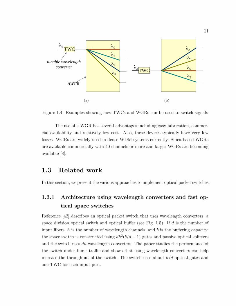
WGRs can be used to switch signals when used in combination with tunable
wavelength converters (TWC). This is shown in Fig. 1.4. Consider a TWC connected
to the ith input of a WGR, 0 ≤ i < h, where h is the number of inputs of the WGR.
If a signal coming in at the TWC is tuned to wavelength k, the signal is routed to
output (i + k) mod h. Thus, a signal arriving at input 0 will be routed to output 3 if
tuned to λ3 (Fig. 1.4(a)) and a signal arriving at input 3 will be routed to output 4
if tuned to λ1 (Fig. 1.4(b).
11
TWCλ0
tunable wavelength converter
λ0
λ1
λ2
λ3
AWGR
(a)
TWCλ2 λ0
λ1
λ2
λ3
(b)
Figure 1.4: Examples showing how TWCs and WGRs can be used to switch signals
The use of a WGR has several advantages including easy fabrication, commer-
cial availability and relatively low cost. Also, these devices typically have very low
losses. WGRs are widely used in dense WDM systems currently. Silica-based WGRs
are available commercially with 40 channels or more and larger WGRs are becoming
available [8].
1.3 Related work
In this section, we present the various approaches to implement optical packet switches.
1.3.1 Architecture using wavelength converters and fast op-
tical space switches
Reference [42] describes an optical packet switch that uses wavelength converters, a
space division optical switch and optical buffer (see Fig. 1.5). If d is the number of
input fibers, h is the number of wavelength channels, and b is the buffering capacity,
the space switch is constructed using dh2(b/d + 1) gates and passive optical splitters
and the switch uses dh wavelength converters. The paper studies the performance of
the switch under burst traffic and shows that using wavelength converters can help
increase the throughput of the switch. The switch uses about h/d optical gates and
one TWC for each input port.
12
TWC
TWC
Spaceswitch
TWC
TWC
λ0
λh
h
h
d d
b/d+1 bufferingexits
Buffer withb positions
λ0
λh
dh × h(b/d+1)demultiplexor
input fibertunable wavelength
converter
Figure 1.5: Optical packet switch with wavelength converters and buffering using aspace switch [42]
1.3.2 Wavelength routing switches
KEOPS (Keys to Optical Packet Switching) [40, 29] was a project that demonstrated
many key building blocks that are necessary to build optical packet switches. The
project demonstrated systems that used transmission rates of 2.5 Gbps and 10 Gbps
per wavelength channel. Two different packet switch architectures were put together
and demonstrated. The first switch architecture is called a wavelength routing switch
and is shown in Fig. 1.6. Each input carries a single wavelength channel and packets
are of a fixed length. In the WDM version with h wavelength channels per fiber, the
switch has h planes of the wavelength routing switch. The first stage of the switch
distributes packets to the various multiplexors in the middle. The second stage routes
the packets to the output ports on wavelengths that are available at the output. The
fiber delay lines after the distribution stage serve as input buffers and they prevent
head-of-line blocking from occurring. The paper presents algorithms to route packets
to the output ports without creating conflicts at the intermediate stages and at the
outputs. This switch needs two stages of wavelength conversion, thus needing 2dh
tunable wavelength converters, where d is the number of input fibers and h is the
number of wavelength channels per fiber.
Optical Label Switching (OLS) is another technology to perform optical packet
switching. It is very similar to OBS in that the control plane operations are performed
13
TWC
TWC
TWC
TWC
tunable wavelength converter
123
TWC
TWC
TWC
TWC
fiber delay lines
Figure 1.6: The KEOPS wavelength routing switch fabric [40, 29]
electronically and the data forwarding is done optically. However, the control header
(label) is sent optically on the same wavelength as the data and the label is extracted
from (or added to) the packet using technologies like sub-carrier multiplexing. Also,
the data payload has to be delayed while the control operations are determined. Ref-
erences [62, 103, 41] describe the implementation of an OLS router. The switch fabric
used is shown in Fig. 1.7. The switch is nonblocking and uses Arrayed Wavelength
Grating Routers (WGRs) in combination with two stages of wavelength conversion,
one of which uses tunable wavelength converters and the other uses fixed wavelength
conversion. The tunable wavelength converter is used to route a packet to the des-
tination port through the WGR. The fixed wavelength converter converts the signal
to a wavelength channel that is not in use at the destination port. It needs a very
large WGR and uses two stages of wavelength converters (2dh wavelength convert-
ers). Reference [41] describes a way to scale the switch while using a small WGR
(256× 256 WGR for a 40 Pbps switch). However, this leads to some blocking within
the switch. In this switch, the cost of wavelength conversion can be a crucial factor
in determining its commercial feasibility.
Reference [108] describes a switch that also uses the wavelength domain to
route data through the switch and the switch is shown in Fig. 1.8. The switch
architecture uses two stages of tunable wavelength converters and three WGRs to
switch the data signals. Also, the switch uses one stage of input buffering or output
14
TWC
TWC
AWGRdh × dh
TWC
TWC
λ0
λh
h
h
d
λ0
λh
FWC
FWC
h
FWC
FWC
h
d
demultiplexor
input fibertunable wavelength
converterfixed wavelength
converter
multiplexor
Figure 1.7: Optical packet switch with wavelength converters and AWGR in an Op-tical Label Switch [103]
TWC
TWC
AWGRK × KTWC
TWC
Input 1
tunable wavelength converter fiber delay lines
Input 2
Input N
AWGRK × K
M-1
2
1
TWC
TWC
TWC
TWC
AWGRN × N
Figure 1.8: Optical packet switch with input buffering capability using wavelengthconverters and WGR [108]
buffering using fiber delay lines to resolve contention. For a system with d input
fibers and h wavelength channels per fiber, the switch uses 2dh tunable wavelength
converters and needs WGRs of the order of dh×dh. Here again, the size of the WGR
needed is not scalable for large systems and the cost of wavelength conversion makes
this switch relatively expensive as compared to electronic routers. The WASPNET
switch [31] also uses two stages of tunable wavelength converters in combination with
a 2dh × 2dh AWGRs. The switch uses a few ports of the WGR to provide buffering
using fiber delay lines.
15
Cou
pler
TWC
TWC
TOF
TOF
FOF
FOF
1 packet delay line
gate
fixed optical filter
tunable optical filter
d outputsd inputs
Figure 1.9: Broadcast and Select switch with a recirculating buffer [35]
1.3.3 Broadcast and Select switch architectures
In broadcast and select architectures, packets from input ports are sent to all output
ports on different wavelengths and each output port chooses the packet that it has to
transmit using a wavelength selective device (like a tunable optical receiver). In gen-
eral, Broadcast and Select architectures can support only a limited number of input
ports (up to the number of wavelength channels) because there would be wavelength
conflicts otherwise. Thus, they are suitable for building switches that have a rela-
tively small aggregate bandwidth. Broadcast and Select switches naturally support
multicasting making them attractive options to build switches that need to support
this capability.
Reference [35] describes a broadcast and select switch with a recirculating
buffer. Each input carries data on some wavelength and packets are of some fixed
length. The number of wavelengths, h, is greater than the number of inputs, d. Each
input signal is tuned to some wavelength using a tunable wavelength converter and
the different signals are combined using a passive coupler and the combined signal is
transmitted to d tunable optical filters and h fixed optical filters. Also, the signals,
that are recirculated, pass through a delay line that can hold one packet in each
wavelength and are then fed back into the coupler. Of the signals in the coupler, up
to d of them are transmitted to the output ports using the tunable filters and up to h
are recirculated back into the coupler. This architecture uses one tunable wavelength
converter and one tunable filter for each input channel. Also, the recirculation buffer
uses h fixed filters and h gates.
16
FWC
FWC
fixed wavelength converter
fiber delay lines
h
1
b
gate
h
h
b
b
Figure 1.10: The KEOPS Broadcast and Select switch [40, 29]
The KEOPS project demonstrated a broadcast and select switch that is shown
in Fig. 1.10. The switch operates on fixed packet lengths. Here again, each packet
is transmitted using a different wavelength into the buffers. Using the gates and the
multiplexors, it can be shown that this switch emulates an output buffered switch
with a buffer capacity of b packets at each output.
1.3.4 Switching in the time domain
Photonic Slot Routing [19, 106] is a time domain switching mechanism where data is
transmitted in fixed length timeslots and the switching is performed across timeslots.
Each timeslot corresponds to a fixed duration of transmission across all wavelength
channels and a timeslot is switched as a whole unit. Hence, all wavelength channels
are treated as a single transmission channel as far as switching is concerned. This
approach is similar to Time Sliced Optical Burst Switching (TSOBS) that we propose
in this dissertation. However, in TSOBS, the timeslots on each wavelength channel
are switched independently. This leads to better utilization of the network bandwidth.
The switch designs discussed for TSOBS could be applied to Photonic Slot Routing
switches.
Terahertz optical asymmetric demultiplexor (TOAD) is a device that can work
as an AND gate and is described in Reference [86]. It has been demonstrated at a
line speed of 100 Gbps. In a demonstration of a single routing node, packets from
slower speed sources were interleaved onto the 100 Gbps link and a bank of TOADs
extract individual streams.
17
1.3.5 Optical switch fabrics in electronic switches
Recently, there has been interest in using optics to build the switch fabric within
an electronic switch because of the capacity offered by optical switches. It has been
identified that the main deterrent to building high speed internet routers is the power
density of the switch fabric racks [65]. By using optics to build the switch fabric,
the power requirement can be reduced and thus, this makes it possible to build very
high speed switch fabrics. Reference [65] describes a design for a switch, that has an
aggregate capacity of 100 Tbps. A key observation, made in the paper, is that a switch
fabric can be built by using a static interconnection of links, each link having twice the
bandwidth capacity as the input link speed. Since optics gives us abundant bandwidth
capacity, the switch uses optics for the interconnection network. The switch uses
MEMS switches used in a static configuration to provide the interconnection network
that is reconfigurable in the face of linecard failures.
Reference [52] describes a switch fabric that is built using tunable lasers and
a WGR to route the signals to the output port. The switch aggregates packets
electronically at the line card and switches them to the output using the switch
fabric as described in Section 1.2.5 (tunable lasers are used instead of wavelength
converters). The paper describes a demonstration that uses four ports each running
at 40 Gbps through a switch fabric that can support an aggregate capacity of 1.2
Tbps.
1.4 Dissertation outline
The problem with the optical switches that have been discussed is that they use
components that are expensive and hence, make the systems expensive relative to
electronic routers. Most designs that use tunable wavelength converters and wave-
length grating routers require two tunable wavelength converters per input channel
and require a very large Arrayed Grating Router to resolve contention. Other designs
require both tunable wavelength conversion and fast optical switches.
The objective of this dissertation is to develop less expensive and more eco-
nomically viable optical switches that can be used in the data path of burst routers.
We propose a design for wavelength converting switches, used in OBS routers, that use
passive wavelength grating routers in place of optical crossbars. This design makes
the switch less expensive because wavelength grating routers are easier to fabricate
18
and are much less expensive than optical crossbars. Also, the size of the wavelength
grating routers needed are determined by the number of wavelength channels used
and not the number of input ports. However, the use of wavelength routers introduces
some blocking in the switch. We model the blocking in the switch through the help of
a combinatorial puzzle or a game and discuss the various research problems involved.
The design of wavelength converting switches is presented in Chapter 2.
We then propose a variant of burst switching called Time Sliced Optical Burst
Switching (TSOBS) that eliminates the need for wavelength conversion by switching
data in the time domain in Chapter 3. Optical time slot interchangers are key com-
ponents that are required to implement time slotted switching. We discuss the design
of time slot interchangers and the scheduling algorithms needed to implement the
required switching operations. Through a cost analysis, we show that that TSOBS
has the potential of being cheaper than electronic routers and is a promising solution
to implement optical burst switching commercially.
Time sliced optical burst switching uses fixed length time slots to switch data.
This requires that the data packets from hosts are of comparable size to a time slot
to maintain good data transmission efficiency. The average size of packets in the
Internet is too small for the time slots used in practical TSOBS networks. Thus,
we need an aggregation mechanism at the network interfaces, that connect hosts to
a TSOBS network. When multiple hosts transmit packets to the same destination
network, we can aggregate the packets to form a “super-packet” that utilizes time
slots more efficiently. We discuss an aggregation algorithm and study its performance
in a TSOBS network in Chapter 4.
In TSOBS networks, since data is switched in the time domain, individual
wavelength channels can get loaded with uneven amounts of data causing a degra-
dation in the network performance. This problem can be alleviated by using load
balancing techniques at the network interfaces where we have the freedom to choose
the wavelength that a burst is sent on. We study four algorithms for addressing this
problem and evaluate their performance in Chapter 5.
19
Chapter 2
Design of Wavelength Converting
Switches
A wavelength converting switch is one that switches data signals that are carried
on a wavelength channel of an input fiber to any wavelength channel of an output
fiber. Wavelength converting switches require wavelength converters to switch the
data across wavelength channels and to provide acceptable statistical multiplexing
performance, the number of wavelength channels needs to be large (at least tens,
preferably hundreds). More details on the statistical multiplexing performance of
optical burst switching can be found in [91].
Each Burst Switch Element (BSE) in a burst switch requires a wavelength
converting switch, capable of switching an optical signal from any of the BSE’s d
input fibers to any of its d output fibers (Fig. 2.1). A BSE with d = 8 and h = 256
wavelengths would have an aggregate throughput of 2 Tb/s, assuming 10 Gb/s per
wavelength.
h wavelengthsper fiber
d input andoutput fibers
Figure 2.1: Wavelength converting switch with d input/output fibers and h wave-length channels per fiber
20
h
TWC
TWC
h
TWC
TWC
dd
Figure 2.2: Wavelength converting switch using Tunable Wavelength Converters(TWC), Optical Crossbars and Passive Multiplexors and Demultiplexors
We describe two designs for wavelength converting switches. The first uses
wavelength conversion in combination with fast optical crossbars to perform the re-
quired switching operations. This switch design is strictly non-blocking. However, the
fast optical crossbars required are expensive components. The second design replaces
the crossbars with Wavelength Grating Routers, which are passive devices, resulting
in a lower cost switch design.
2.1 Switch Based on Optical Crossbars
Fig. 2.2 shows the first wavelength converting switch design. Each of the d input
sections has an optical demultiplexor that separates the different wavelength channels
from each other before propagating through Tunable Wavelength Converters that
quickly tune to any of the h output wavelengths. The wavelength converters are
followed by h × d crossbars. Outputs of each crossbar are then connected to distinct
passive multiplexors, which constitute the output section of the switch. The crossbars
can be decomposed into d × d sections, followed by additional passive multiplexors,
reducing the required size of individual crossbar components. Note that the crossbars
implement a combination of switching and multiplexing, since there may be several
signals on a given input fiber that are propagated to the same output fiber. If they
are converted to distinct wavelengths, these signals may share the same crossbar
output, so long as the optical crossbar technology is designed to support this. SOA-
based crossbar technology is capable of implementing this combined switching and
multiplexing function.
To route an incoming burst to an output, the input wavelength is converted
to any available wavelength at the required output, and the crossbar is configured
to propagate the signal to the required output. The switching and multiplexing
capability of the crossbar ensures that there is no blocking, so long as there is an
available wavelength on the selected output. Because burst arrival is unpredictable,
there will be times in an OBS router when no output wavelength is available for
an arriving burst. In routers with no internal buffering, such bursts are discarded.
Fortunately, with high channel counts, the probability of burst discards is very low.
As this design requires both tunable wavelength converters and high-speed
crossbars, the cost of the system is relatively high and may make it impractical for
commercial systems. However, the design is strictly nonblocking making it a good
choice for comparison with other switch designs.
2.2 WGR-Based Switch Design
The WGR-based switch design we are interested in is shown in Fig. 2.3. Each of
the d input sections consists of four components, an optical demultiplexor, a bank
of tunable wavelength converters, a wavelength grating router and a bank of optical
22
multiplexors. The router and the multiplexors are joined through a fixed permutation
pattern. We will see that the blocking characteristics of the switch depend critically
on the choice of this permutation pattern. Each output section consists of a single
optical multiplexor. Each input section is connected to each output section by an
optical fiber carrying up to h optical signals on different optical wavelengths. Since
each wavelength can be used only once on each output fiber, the signals arriving at
an output section from different input sections must use distinct wavelengths.
In high performance optical networks, hundreds of different optical signals may
be carried on a single fiber, using different wavelengths of light. The optical demulti-
plexor in each input section separates these signals, so that they can be individually
switched to different output fibers. The tunable wavelength converters use a tunable
laser and an optical modulator to transfer the information carried on one input wave-
length to a different (and dynamically selectable) output wavelength. This wavelength
conversion is needed to allow input signals on different input fibers to be switched to
the same output fiber, even if the input signals are carried on the same wavelength.
The wavelength grating router is a passive optical device that switches optical signals
based on their wavelength. Specifically, an optical signal carried on wavelength i at
input j is switched to output (j + i) mod h where h is the number of wavelengths.
Thus, the choice of wavelength used for a given signal determines which output section
the signal is forwarded to. A demonstration of a combination of tunable wavelength
converters and wavelength routers has been discussed in Reference [96].
In this construction, there are h/d different wavelengths that can be used by a
given input signal to reach a particular output, but different inputs may use different
sets of wavelengths to reach the same output. The permutation patterns used in
each of the input sections determine these wavelength sets. To reach an output fiber,
the wavelength converter at the input is tuned to one of these wavelengths and the
incoming signal is “steered” to the required output through the wavelength router. In
this design, the wavelength converters play the dual role of selecting the free output
wavelength as well as providing the required space switching through the switch.
Since a given input channel is not able to use any wavelength to reach a given
output fiber, blocking can occur. That is, there may be situations where all of the
wavelengths that can be used to get to a desired output are in use at the output,
causing blocking to occur even when there are free wavelengths available on the
outgoing link. In the next section, we present this blocking problem as a puzzle on
23
a game board in order to make the nature of this blocking problem more apparent,
and to clarify the issues that affect the blocking performance.
2.3 Design of WGR-based switches
In this section we study the routing problem in WGR-based switches and show how
the blocking performance of these switches is affected by the permutation pattern
used within each of the input sections of the switch.
2.3.1 Routing Multiple Channels Simultaneously
The problem of simultaneously routing a set of channels through a WGR-based switch
can be formulated as a combinatorial puzzle. This formulation makes it easier to
understand the intrinsic structure of the problem, yielding insights that are useful in
design and analysis.
The puzzle is played on a game board made up of dh2 squares arranged in h
columns and dh rows. The board is divided into d square blocks of h rows each. Each
square has one of d different colors, with each row containing h/d squares of each
color and each column containing h squares of each color. To setup the puzzle we
place colored tokens beside some or all of the rows. A setup can include at most h
tokens of any color. An example of a setup game board with d = 2 and h = 8 is
shown in Fig. 2.4(a). To solve the puzzle, we must place each token on a square of
the same color, in the row where the token was placed. The token placement must
also satisfy the constraint that no two tokens of the same color be placed in the same
column. An example solution to the puzzle is shown in Fig. 2.4(b).
Each row in the puzzle corresponds to one of the h input channels on one of the
d input fibers. More specifically, row i in block j of the game board corresponds to
input channel i of input fiber j. The color of the token that is placed by a row corre-
sponds to the output fiber that the corresponding input channel is to be switched to.
More specifically, placing a token of color r on row i of block j corresponds to switch-
ing channel i of input fiber j to output fiber r. The columns of the array correspond
to different output wavelengths. Placing a token in a particular column corresponds
to choosing that output wavelength. The color of each square corresponds to the out-
put that is reached if the wavelength converter for the input channel corresponding
to that square’s row is tuned to the wavelength corresponding to the column. So,
24
(a) Example puzzle setup (b) Example solution
Figure 2.4: An example puzzle setup and solution
placing a token of color r in column q of row i of block j corresponds to switching
channel i of input fiber j to channel q of output fiber r. Note that the puzzle rule
requiring that no two tokens of the same color occupy the same column corresponds
to the requirement that no two input signals going to the same output fiber use the
same wavelength.
In order to complete the correspondence between the puzzle and the routing
problem, we note that within each block the rows must have closely related color
patterns, in order to model the routing characteristics of the WGRs. Specifically, the
pattern of colors within each row can be obtained from the previous row’s pattern by
a cyclic rotation of one column. This relationship only holds within each block. There
is no requirement that different blocks have similar color patterns. The color pattern
for each block corresponds to the permutation pattern within the input sections of
the switch. This is illustrated in Fig. 2.5 which shows two example configurations of
a system with d = 2 and h = 8 and the corresponding game boards.
Whenever the puzzle has a solution, it means that there is a way to route the
input signals to the output channels that are specified by the tokens placed by each
row. If the puzzle does not have a solution, then there is no way to route all the
channels simultaneously. If, for all possible puzzle setups, there is a solution, the
25
wav
elen
gth
rout
er (
8x8)
wav
elen
gth
rout
er (
8x8)
(a)w
avel
engt
hro
uter
(8x
8)w
avel
engt
hro
uter
(8x
8)
(b)
Figure 2.5: Two configurations and the corresponding game boards of a system withd = 2 and h = 8
switch is rearrangeably non-blocking. It is easy to see that the switch in Fig. 2.5a is
not rearrangeably non-blocking, since the puzzle setup in which tokens of one color
are placed in even-numbered rows and tokens of the other color are placed in odd-
numbered rows has no solution. On the other hand, this setup does have a solution
when played on the game board in Fig. 2.5b.
To generalize the problem of routing connections simultaneously, we restrict
the number of tokens of a particular color to some value k ≤ h.
Definition 2.3.1 A game board is k-solvable if every puzzle setup with at most k
tokens of each color has a solution.
We show below that no game board is h-solvable. Fortunately, in practice, it
can be sufficient to find game boards that are k-solvable for values of k fairly close to
h.
26
2.3.2 Routing problem as a bipartite matching problem
The problem of solving the puzzle can be reformulated as a matching problem in a
bipartite graph. We start by constructing the bipartite graph. The graph consists
of two subsets of vertices; let us call them the “left” and “right” subsets. The “left”
subset includes vertex u(i, j) that corresponds to row j in block i of the game board (or
channel j of input fiber i). The “right” subset includes a node v(q, r) that corresponds
to color q and column r (or channel r of output fiber q). We include the edge
{u(i, j), v(q, r)} in the graph if the color of the token in row j of block i is q and
the color of the square in column r of row i and block j is q. In terms of the WGR
switch, you include the edge if the signal on input fiber i, channel j is to be switched
to output fiber q, and you can reach output fiber q using wavelength r.
In each row of the game board, there are h/d squares of the color corresponding
to output q or h/d wavelengths that switch signals to output q. Thus, for each token
that is placed at row j of block i, there are h/d edges that are drawn from the “left”
subset to the “right” subset. One observation about this graph is that it breaks apart
into separate subgraphs corresponding to the different outputs. This just corresponds
to the fact that the placement of tokens of one color is independent of the placement
of tokens of other colors.
This is illustrated in Fig. 2.6(a) for a system with 2 input fibers and 8 wave-
lengths per fiber for one output. The token placed in the second row of block 0 has
four squares of the same color as the token in columns 1, 4, 5, and 7 respectively. This
results in 4 edges in the bipartite graph from vertex (0, 1) to vertices corresponding
to λ1, λ4, λ5, and λ7 at the output. Similarly, 4 edges are drawn from vertex (1, 3) to
vertices corresponding to λ2, λ3, λ5, and λ7 at the output. This is repeated for each
token placed beside the game board.
Now find a maximum size matching in this bipartite graph. If there is an
edge for every token, you have a solution. In particular, if {u(i, j), v(q, r)} is in the
matching, then put the token in block i and row j in column r (equivalently, tune the
wavelength converter for channel j of input fiber i to output wavelength r). Using a
well-known maximum size matching algorithm based on max flows in unit networks,
one can solve the puzzle in O(h5/2) time, assuming a solution exists.
A maximum size matching for the bipartite graph in the example is shown
in Fig. 2.6(a). Note that one of the left vertices, (1, 7), cannot be matched to any
output vertex because there does not exist an available vertex at the output that can
be matched to this vertex. Given the matching in the graph, we can place the tokens
27
Unmatched vertex
Input 0
Input 1
λ0λ1
λ2
λ3λ4
λ5
λ6
λ7
(0,1)
(0,7)
(1,3)
(a)
Token cannot be placed
(b)
Figure 2.6: (a) Example bipartite graph formulation of a puzzle; (b) Solution topuzzle
on the game board as shown in Fig. 2.6(b). For example, token (0, 1) is placed in the
second column of the game board corresponding to λ1, token (0, 7) is placed in the
fourth column, and token (1, 3) is placed in the eighth column respectively.
The connection with matching also yields an algorithm for rearranging existing
connections to accommodate new ones, which corresponds directly to the augment-
ing path algorithm for bipartite graphs. This can be described in terms of the game
board as follows. If it is not possible to place a token of color x in row r1 (satisfy-
ing the required constraints), then find an “x-augmenting path” in the game board
starting at some square of color x in row r1. Call this square (r1, c1) where c1 is the
column number. An x-augmenting path in the game board is a sequence of squares
(r1, c1), (r2, c2), (r3, c3), ..., (rm, cm) satisfying the following properties:
• All squares in the sequence have color x.
• Squares (r2, c1), (r3, c2), ..., (rm, cm−1) all contain a token of color x.
• There is no token of color x in column cm.
28
Given such a path, we place a token on (r1, c1) and for 1 < i ≤ m we move the token
on square (ri, ci−1) to (ri, ci).
We can find such a path by performing a breadth-first search through the game
board. We construct the search tree as follows. The nodes, Ni (1 < i ≤ hd), of the
tree correspond to the rows of the game board. To place a token of color x in row
r1, let Nr1 be the root node of the tree. If column c in row r1 has a square of color x
and row rk has a token of color x in column c, then we add an edge from Nr1 to Nrk
in the tree. There are h/d nodes adjacent to node Nr1 . We can construct the tree by
recursively adding nodes at distance 1 from the newly added nodes. The search stops
when we have a row that has a column with no token of color x placed in it; that is,
we can move the token in the row to this free column.
Note that once a node Nrihas been added to the tree, another node corre-
sponding to the same row ri will not be added at a lower level. This is because the
subtree at both the nodes will be the same and the augmenting path is the shortest
through the first instance of the node (since this is a breadth-first search). The search
can stop without finding an augmenting path. This happens when none of the nodes
in the tree has a column of color x with no token placed in it and we cannot add more
nodes to the tree (other than nodes corresponding to rows that have already been
added). In this case, the new token cannot be placed on the board and the puzzle
cannot be solved.
Fig. 2.7 illustrates the rearrangement algorithm for a system with d = 3 and
h = 9. Fig. 2.7(a) shows the state of the system before the placement of a token at
(1, 2). The game board configuration shows only the first two blocks. We assume
that the last block does not have any tokens placed on it. Also, only the squares
corresponding to the output we are interested in are represented by the dark squares.
The other 6 squares (light colored squares) in each row correspond to the other two
output fibers and the row configuration for them does not affect the token placement
for the output we are interested in.
To place the token, we start a breadth first search starting with the row we
want to place the token in, (1, 2), as the root node. The columns that this row can
use to reach the output are 0, 3, and 7. All three columns are occupied by other
rows. The algorithm searches for a free column in rows that have tokens in the above
columns. Thus, (0, 0), (0, 6), and (0, 2) are added as the first level nodes in the search
because they have tokens in columns 0, 3, and 7 respectively. The columns that the
two rows share are indicated beside the edge in the graph. All three rows do not
29
0 1 2 3 4 5 6 7 8
(a)
(0,6) moved to column 8
(1,2) placed in column 3
(1,3) moved to column 6
0 1 2 3 4 5 6 7 8
(b)
1,2
0,6
1,3
0,0 0,2
1,0 1,6 1,6
0
2 5
37
85
(1,3) has a free column to move token
(c)
Figure 2.7: (a) Game board before placing token; (b) Rearrangement to place newtoken; (c) Breadth first tree to rearrange tokens on the game board
have free columns to move their tokens to. The algorithm searches one more level of
nodes. Row (0, 0) shares columns 2 and 5 with rows (1, 0) and (1, 6) respectively and
neither of these has a free column. So, the algorithm adds nodes (1, 0) and (1, 6) as
children of node (0, 6) in the tree. Row (1, 3) shares the column 8 with row (0, 6) and
column 6 is available. Thus, the search terminates and we have an augmenting path
((1, 2), 3), ((0, 6), 8), ((1, 3), 6). The breadth first tree is shown in Fig. 2.7(c). The
token in row (1, 3) is moved to column 6, the token in row (0, 6) is moved to column
8, and the new token is placed in column 3 of row (1, 2). Fig. 2.7(b) shows the game
board after the token is placed.
30
2.4 Finding Good Game Boards
The design of the game board has a big influence on our ability to solve the puzzle.
Since the game board design corresponds to the permutation pattern of the input
section, this means that the permutation pattern affects the likelihood of blocking.
The game board in Fig. 2.5a has many puzzle setups that have no solution, making it
a poor design, from the perspective of the puzzle solver. What makes it a poor design
is that many rows have exactly the same pattern of colors. This means that if tokens
of the same color are placed in these rows, the number of columns they have to choose
from is limited, and may be smaller than the number of tokens. This suggests that a
good game board design will be one in which different rows have different patterns,
and in particular, have as few columns in common as possible with squares of the
same color.
Definition 2.4.1 A cover of some row, say i, for some color “blue” is defined as the
set of columns that have a blue square in row i in the game board.
The cover of a set of rows R is defined as the union of the covers of each of
the rows that is contained in the set R.
A game board is k-solvable if and only if in each of its associated bipartite
graphs, there is a matching of size t between any set of t ≤ k inputs and all its outputs.
By the well-known Marriage Theorem for bipartite matching, such a matching exists
if and only if every set of t ≤ k nodes in the “left” subset has at least t neighbors in
the “right” subset. We can restate this in terms of the puzzle, as follows. A game
board is k-solvable if and only if for all colors j and all r ≤ k, all sets of r rows cover
at least r columns.
2.4.1 Upper bounds on puzzle solvability
We first show that no game board is h-solvable. Consider an arbitrary game board
and color blue. There are exactly h blue squares in any column of the game board,
meaning that there are dh − h squares that are not blue. If we select any h rows
from among the dh−h rows that do not have blue squares in the given column, then
any puzzle setup that has blue tokens in these h rows is unsolvable, since none of the
tokens can be placed in the selected column, and we must place each of the h tokens
in a distinct column. Similarly, if we consider any i ≤ d − 1 columns, there must be
at least (d − i)h rows that do not contain blue squares in any of these columns. So,
31
any puzzle setup that has blue tokens in more than h− i of these rows is unsolvable.
These results make it clear that we cannot expect to construct a WGR-based switch
that will guarantee our ability to place more than h − d + 1 tokens of the same
color. Fortunately, the value of h is typically much larger than d for configurations of
practical interest, which means that the degree of blocking implied by this limitation
may be acceptable. This gives us
Theorem 2.4.2 For any k-solvable game board on d colors and h columns, k ≤h − d + 1
For larger values of d, we can get a stronger bound using the following theorem
which is proved in Reference [82].
Theorem 2.4.3 Let G be a game board on d colors and h columns and let s be any
integer that satisfies
dh(h − (h/d)
)s/hs ≥ h − s + 1
where xr = x(x − 1) . . . (x − r + 1). If G is k-solvable, then k ≤ h − s − 1.
Fig. 2.8 shows the upper bound of the number of tokens that can placed as
a function of the number of wavelengths, h, for various values of d. For h = 256
and d = 8, 15 is the largest value of s that satisfies the inequality, giving a limit of
240 on the solvability of game boards with h = 256 and d = 8. If we increase d to
16, the largest s increases to 41 and the limit becomes 214. If we fix a value of d
and let h → ∞, the theorem implies that k ≤ h − �logd/(d−1) d�. Since logd/(d−1) d
is roughly d ln(d) for larger values of d, we can use h − d ln d as an estimate of the
bound, which for larger values of d is significantly smaller than the h− d + 1 implied
by Theorem 2.4.2. However, for h >> d, even this stronger bound does not rule out
the existence of practically useful game boards.
2.4.2 Contiguous game boards
A repetitive game board is a game board whose d blocks are the same. A contiguous
game board is a repetitive game board in which the first row of each block is divided
into d contiguous monochrome blocks of size h/d each. Remarkably, for d = 2,
contiguous game boards are h− 1 solvable. To see this, fix a color and note that any
set of i rows in the same block covers at least (h/d) + i − 1 columns. Any set of k
rows in the game board must have at least �k/d� rows in some block, and so must
32
0
100
200
300
400
500
0 100 200 300 400 500
Number of wavelengths (h)
Up
per
bo
un
d o
n s
olv
abili
ty
d = 16
d = 8
d = 4 d = 32
Figure 2.8: Upper bound on the solvability of game boards
k k
Row 1
Row k
Columns shared by the rows
Figure 2.9: Example showing rows sharing columns
cover at least (h/d) + �k/d� − 1 columns. For k = h − 1, this is 2(h/d) − 1, which is
h − 1 when d = 2. That is, a contiguous game board with d = 2 is (h − 1)-solvable,
matching the upper bound in the previous sub-section. For arbitrary values of d, we
have the following theorem from Reference [82].
Theorem 2.4.4 A contiguous game board on h columns with d colors is k-solvable
if and only if k−�k/d� ≤ h/d− 1. The largest value of k that satisfies this condition
is
k∗ =
{(h/(d − 1)) − 1, if d − 1 divides h/d,
(h/(d − 1)) − (h/d mod d − 1)/(d − 1), otherwise.
The first part of the theorem follows directly from the discussion above. The
second part can be shown by substitution.
33
2.4.3 Random Game Boards
We now show how random game boards can be good choices for constructing switches
with good blocking performance. Any row in a game board has h/d squares of the
same color. When two or more rows have a square of the same color in a column,
the column is said to be shared by the rows. The number of columns covered by any
two rows in a game board is 2h/d minus the number of columns that are shared by
these rows. Consider any two rows in the same block of the game board, row 1 and
row k, without loss of generality. By the construction of the game board, row 1 is
circularly shifted k squares to the left to obtain row k. Suppose row 1 has a square
of some color in column i and a square of the same color in column i + k, then row
k has a square of the same color in column i because the square in column i + k in
row 1 moves to column i in row k when shifted left by k squares. Thus, the two rows
share the ith column. In general, the number of columns shared by row 1 and row k
is the number of pairs of squares that are at a distance of k from each other in row
1. Fig. 2.9 illustrates this.
To construct good game boards, we need to maximize the number of columns
covered by any set of rows. This is equivalent to minimizing the number of columns
shared by the set of rows. Thus, we need to minimize the number of pairs of squares
that are at a distance k from each other, for all values of k. Regular constructions of
game boards can minimize the number of columns shared by rows for some values of
k but may do poorly for other values of k. Randomizing the positions of the squares
within a row can be expected to spread the distances between pairs of squares across
all possible values. This reduces the number of columns shared by all possible row
sets.
Our criterion for a good game board is one in which any set of r rows covers at
least r columns, for each color. For larger values of h and d, we can expect random
game boards to do well, in this respect. Consider an arbitrary set of r rows within
a single block of a random game board. The probability that a particular column is
not covered for some fixed color is
h − r
h
h − r − 1
h − 1. . .
h − r − h/d + 1
h − h/d + 1=
(h − r)h/d
hh/d
34
1.E-06
1.E-05
1.E-04
1.E-03
1.E-02
1.E-01
1.E+00
1.E+01
1.E+02
0 50 100 150 200 250number of rows
E(n
umbe
r of
unc
over
ed c
olum
ns)
d=2 4
32
16
8
64
tolerable number of uncovered columns
Figure 2.10: Number of columns not covered by row sets of all sizes (h = 256)
Thus, within one block, the expected number of columns not covered by r rows is
h(h − r)h/d
hh/d
The expected number of columns not covered by r rows selected from d independent
random blocks in the game board is
= h(h − r1)
h/d
hh/d
(h − r2)h/d
hh/d.....
(h − rd)h/d
hh/d
≤ h
((h − r/d)h/d
hh/d
)d
where r = r1 + r2 + . . . + rd, and ri is the number of rows in the ith block of the
game board. The expected number of columns not covered is plotted as a function of
the size of the row set, r in Fig. 2.10. The expected number of columns not covered
gives us an upper bound on the probability that a given set of rows fails to cover one
or more columns. In the figure, the curve labeled “tolerable number of uncovered
columns” is h minus the size of the row set.
For the values of d of most practical interest (≤ 16), the number of columns not
covered by any random row set is much less than the tolerable number. For d = 8, the
probability that a set of 140 or more rows fails to cover any column is less than one in
a million. Another way to look at this is to note that while a nonblocking switch can
implement all mappings of the input channels to output links, the blocking switch
can implement all but a minuscule fraction of the set of possible mappings.
35
Token cannot be placed
Figure 2.11: Example showing that a blocker with more than h/d tokens of somecolor can beat a naive setter
2.5 Routing Connections Online
The puzzle introduced above corresponds to the version of the routing problem in
which we are asked to simultaneously route a whole set of connections. More often,
we are interested in routing individual connections one-at-a-time, without disturbing
connections routed previously. This problem can be formulated as a two player game,
played on the same game board as the puzzle.
Let’s call the first player the blocker and the second player, the setter. The
blocker is given k ≤ h tokens of each of the d different colors. The blocker takes a
turn by removing zero or more tokens from the board and placing one token beside
some unoccupied row of the board. The setter takes its turn by placing the token put
down by the blocker, in a square of the same color as the token in the selected row.
When placing the token, the setter must not use any column that already contains a
token of the same color. The blocker wins if the setter is not able to place the token
on the board without violating the conditions. The blocker loses if the setter is able
to keep the game going indefinitely.
The switch is strictly nonblocking if no matter how badly the setter plays, there
is no way for the blocker to force a win. The switch is wide-sense nonblocking if there
is a winning strategy for the setter (that is a strategy that will keep the game going
forever, regardless of how well the blocker plays).
36
X=0 X=1 X=2 X=h
λ0 λ1 λ2 λh-1
µ 2µ 3µ hµ
Figure 2.12: Birth-death modeling an output of the switch
Since a winning strategy for the setter would imply that the corresponding
puzzle always has a solution, we cannot expect a winning strategy in versions of
the game where the blocker has more tokens than allowed by the upper bounds in
Section 2.4. It’s easy to see that the setter has a trivial winning strategy when the
number of tokens of each color is limited to ≤ h/d. Hence, the switch is strictly
nonblocking in these cases. It’s also easy to see that the blocker can beat a naive
setter if the blocker is allowed more than h/d tokens of each color. This is illustrated
in Fig. 2.11. The blocker just needs to get the setter into a state where the h/d
columns of some row are already being used by other tokens. In Fig. 2.11 the new
token cannot be placed because the columns it can use to place the token are already
in use by other tokens. In other words, the switch is strictly nonblocking if and only
if the blocker is limited to ≤ h/d tokens of each color.
We now present an approximate analytical model for evaluating the perfor-
mance of wavelength converting switches in OBS routers. The performance metric
used is the fraction of arriving bursts that must be discarded. This is called the burst
rejection probability. We phrase the model in terms of the game board. Since the
tokens of different colors are independent, we focus on tokens of a single color. New
tokens arrive at rate λ, and if possible are placed on the game board. Tokens stay on
the game board for an average time period of 1/µ. If the token interarrival time and
the token “dwell time” are exponentially distributed, we can model the system by
the birth-death process shown in Fig. 2.12, where the state index corresponds to the
number of tokens on the game board. The transition rate from state i to state i − 1
is iµ, where 1/µ is the expected time duration for which a token stays on the game
board. The transition rate from state i to i + 1 varies for different states since the
probability that an arriving token is actually placed on the game board decreases as
the number of tokens on the board increases. The rate, λi, is the rate at which tokens
are placed on the board, and is equal to λ times the probability that an arriving
token is successfully placed. So, for i < h/d, λi = λ. For i ≥ h/d and a random game
37
board, we can approximate λi by
λi = λ
(1 −
(h − h/d
i − h/d
)/
(h
i
))
Note that(
hi
)is the number of sets of columns that can be used by i tokens and(
h−h/di−h/d
)is the number of column sets used by i tokens that would prevent placement
of a new token.
If we let πi be the steady state probability that the system is in state i, then
it can easily shown that
πi =λ0λ1 . . . λi−1
i! µiπ0
Using π0 +π1 + . . .+πh = 1 and solving for π0, we can determine the individual
steady state probabilities. The burst rejection probability is then given by
Prejection(ρ) =h∑
i=h/d
πi
(h − h/d
i − h/d
)/
(h
i
)
where ρ is the offered load to the system given by λ/hµ and(
h−h/di−h/d
)/(
hi
)is the prob-
ability of a burst being rejected in state i.
2.5.1 Simulation results for random game boards
We now study how the blocking characteristics of the WGR-based switch affects the
statistical multiplexing performance of an OBS router using simulation and compare
the results with the analysis.
Here, we consider only the case of routers in which there are no buffers available
to store bursts which can’t be routed to the proper output without a wavelength
conflict. Burst arrivals on each input channel are independent and each arriving
burst is randomly assigned to a different output fiber. Burst lengths and the idle
times between successive bursts on the same channel are exponentially distributed.
The simulations used random regular permutation patterns at the input sections of
the switch. Arriving bursts are assigned to a random wavelength that takes them to
the proper output that is not already in use at that output.
The burst rejection probabilities for systems with different values of d and h and
varying loads are shown in Fig. 2.13. Also shown are the burst rejection probabilities
for systems that use strictly nonblocking switches in place of WGR-based switches.
38
1.E-06
1.E-05
1.E-04
1.E-03
1.E-02
1.E-01
1.E+00
0.35 0.45 0.55 0.65 0.75 0.85 0.95Load
Bur
st R
ejec
tion
Pro
babi
lity
h=64
h=128
h=256
h=128h=256
strictlynon-blockinganalytical
Figure 2.13: Burst rejection probabilities of different system configurations (d = 8)
1.E-06
1.E-05
1.E-04
1.E-03
1.E-02
1.E-01
1.E+00
0.35 0.45 0.55 0.65 0.75 0.85 0.95Load
Bur
st R
ejec
tion
Prob
abili
ty
contiguous
interleaved
random
hand-tuned
non-blocking
Figure 2.14: Burst rejection probabilities of different game boards (d = 8,h = 256)
For a system with d = 8 and h = 256, the rejection probability is 10−6 at a load of
approximately 0.62 for the WGR-based switch and at a load of 0.75 for the strictly
nonblocking switch. For systems designed to operate with a burst rejection ratio
of 10−6, the WGR-based switch can provide a throughput which is approximately
82% of what the nonblocking switch can provide. We also show the burst rejection
probabilities as determined by the analysis of the burst switch. The analysis is pretty
accurate as can be seen in Fig. 2.13.
39
2.5.2 Effects of game board configurations
The next set of results show how different game board configurations can affect system
performance. Fig. 2.14 shows the result of using four different configurations for a
system with d = 8 and h = 256. The first configuration corresponds to a “contiguous”
permutation pattern, wherein, each input block’s first h/d outputs are connected to
the first output, the next h/d outputs are connected to the second output, and so on.
The second configuration corresponds to a perfect shuffle between the wavelength
router stage and the input side couplers. The third configuration corresponds to
a randomly generated game board. The fourth configuration is a hand generated
configuration where colors corresponding to any output in a row are distributed such
that two rows have very little overlap and hence, the number of wavelengths available
to reach a given output between a set of rows is increased. As can be seen from Fig.
2.14, the first two configurations perform poorly. This is because they do not try to
maximize the number of wavelengths available to a subset of input rows uniformly.
The fourth configuration performs slightly better than the random pattern and has a
burst rejection probability of 10−6 at a load of 0.65. With this design, the WGR-based
switch achieves 87% of the throughput that is achieved with the strictly non-blocking
switch.
2.5.3 Effect of reconfiguring connections in the switch
The simulations described above were done with the restriction that once assigned to
a wavelength channel, a burst occupies that wavelength for its entire duration. We
also simulated a situation in which bursts could be dynamically switched to different
wavelengths to accommodate newly arriving bursts. Although this is not a realistic
scenario, it allows us to separate the effects due to the intrinsic blocking character of
the WGR-switches from those due to the restriction on rearrangements. The simu-
lations were done using the rearrangement algorithm described in Section 2.3.2. The
burst rejection probabilities in these simulations matched the strictly non-blocking
results almost exactly for the given traffic pattern. This confirms the implications of
Fig. 2.10. Even though the WGR-based switch is not rearrangeably nonblocking, it
performs nearly as well as a rearrangeably nonblocking switch, when rearrangements
are allowed. This suggests that a better wavelength assignment strategy (the strat-
egy used by the setter to place tokens on the game board) may help reduce the burst
rejection probabilities further, when rearrangement is not allowed.
40
2.5.4 Effect of the wavelength assignment algorithm
In an OBS router, bursts can arrive at unpredictable times and we need to be able
to find an available wavelength at the output to send the burst out on. In a strictly
non-blocking switch, it is sufficient to select any available wavelength at the output
and as long as there are no more than h bursts that need to be routed to an output
at any time, where h is the total number of wavelength channels per fiber, there will
be no blocking. However, we have shown that there is blocking in the switch design
we are interested in. Thus, we need to try to minimize the blocking in the switch by
appropriately routing any burst through the wavelength channel that maximizes the
probability of other bursts that arrive in the future having wavelengths available at
the outputs. In the game formulation described in 2.5, this translates to defining a
strategy for the setter to place tokens on the game board.
Note that the wavelength assignment does not play a role in determining the
performance for the interleaved game board configuration. In this configuration, if a
set of rows share some column in the game board, they share all h/d columns. So, it
does not matter which column we place the token in.
To obtain the results presented in Section 2.5.1, experiments on the game
boards were performed by using a random available wavelength assignment algorithm.
In this algorithm, the arriving burst is assigned to a random wavelength channel at the
output that is unused. We examined three other wavelength assignment algorithms.
Two of those algorithms, first available wavelength assignment algorithm and least
affecting wavelength assignment algorithm, did not yield better performance than the
random available wavelength assignment algorithm. The most available wavelength
assignment algorithm resulted in a much improved performance for the contiguous
board configuration and marginal improvement in the performance for the random
and hand-generated game boards.
First available wavelength assignment algorithm
The first available wavelength assignment algorithm picks the first wavelength at
an input that is not already in use at the output. This corresponds to placing the
token in the leftmost square in the game board that is available. We performed
experiments with a switch with 8 input/output fibers (d), 256 wavelengths per fiber
(h) and random traffic with exponentially distributed interarrival times and burst
41
Available columns
Free rows0 1 2 3 4 5 6 7
New darktoken
Three rows affected by column 2
Two rows affected by column 6
0123456701234567
Figure 2.15: Least affecting wavelength assignment example
lengths. The first available wavelength assignment algorithm did not perform any
better than the random available wavelength assignment algorithm.
Least affecting wavelength assignment algorithm
When a token of some color is placed by the setter in a column of some row, the
column cannot be used to place tokens in the other h − 1 rows that have squares of
the same color. This does not affect rows that are occupied with a token placed in
them (each row can have only one token placed in them at a time). However, the
unoccupied rows get affected by losing one column that could have been used to place
a token when it arrives. Thus, when the token needs to be placed by the setter in
some row, we first find the columns that are available. For each available column,
we count the number of unoccupied rows that get “affected” by choosing this column
for token placement. The least affecting wavelength assignment algorithm places the
token in a column such that the least number of unoccupied rows get affected.
To illustrate the algorithm, let us assume that the state of a switch is as
represented by the game board with h = 8 and d = 2 shown in Fig. 2.15. We consider
connections to the output that has colored squares (as opposed to white squares) and
let us assume that tokens to the output have already been placed as indicated in the
figure. Denote rows as (i, j), where i represents the block and j represents the row
within the block. If we have to place a dark token in row (1, 4), we have two columns,
42
column 2 and column 6, that are available. Also let us suppose that inputs (0, 2),
(0, 3), (1, 0), and (1, 6) are currently free. By choosing column 2, we are reducing
the number of wavelengths available to three rows, (0, 3), (1, 0), and (1, 6), by one.
However, choosing 6 reduces the number of wavelengths available to only two rows,
(0, 2) and (1, 0), by one. Thus, the least available wavelength assignment algorithm
picks column 6.
To evaluate the performance of the algorithm, we performed experiments for a
switch with 8 input/output fibers and 256 wavelengths per fiber and random traffic
with exponentially distributed interarrival times and burst lengths. It was observed
that the performance of the least affecting wavelength assignment algorithm is com-
parable to the performance of the random available wavelength assignment algorithm.
The problem with the algorithm is that it does not ensure that all rows have columns
that can be used to place tokens. In the example shown in Fig. 2.15, row (0, 2) has
only one column (column 6) available where a dark token can be placed. Placing the
token at row (1, 4) in column 6 results in row (0, 2) having no columns available to
place a dark token. Thus, if a dark token is placed beside row (0, 2) by the blocker, the
setter will not be able to place it on the game board. In other words, a burst arriving
at input (0, 2) will have to be dropped because there are no available wavelengths to
route the burst through the switch.
Effect of using most available wavelength assignment algorithm
We now present a routing algorithm that attempts to maximize the number of wave-
lengths available to free inputs to any output and study the effects of using the
algorithm on the performance of the switch.
Define availability, aij, of a row i for color j to be the number of columns that
have a j-colored square and are available in the row and we define these columns to
be available columns. Equivalently, aij is the number of wavelengths at an input i
that take us to output j and are not used by any other input.
Let us suppose a token of color m needs to be placed in row n. If c1, c2, . . . , ck
are the available columns in row n that have an m-colored square (That is, anm = k),
we need to make a choice among one of the k available columns. Let i1, i2, . . . , is
be the rows that are free currently in the game board and ai1m, ai2m, . . . , aism be
their availabilities for color m. If we place the token in column cl, the availability
of rows that have cl as an available column gets decremented by one. Let the new
43
Available columns
Availability of free rows
2
4
3
3
Free rows0 1 2 3 4 5 6 7
New darktoken
Figure 2.16: Switch state for routing example
availabilities be ali1m, al
i2m, . . . , alism, where
alikm =
{aikm − 1 if cl is an available at row ik
aikm otherwise
Now we can define the availability vector, Acl, of a column, cl, as the ordered
vector of the resultant availabilities of the free rows if cl is the column that is chosen
for a new token in row n. That is
Acl= Sort(al
i1m, ali2m, . . . , al
ism)
Among the columns cl, 1 ≤ l ≤ k, we choose the column that has the maximum
availability, where the maximum availability is the lexicographic maximum of all the
availability vectors. Specifically, if A = {a1, a2, . . . , ax} and B = {b1, b2, . . . , bx} are
two availability vectors then
A > B if ∃i ≤ x, such that a1 = b1, . . . , ai−1 = bi−1
and ai > bi
By choosing the column with the maximum availability, we maximize the number of
options available to the row with the minimum number of options for placing tokens
of color m.
44
1.E-06
1.E-05
1.E-04
1.E-03
1.E-02
1.E-01
1.E+00
0.5 0.6 0.7 0.8 0.9 1Load
Bur
st R
ejec
tion
Pro
babi
lity Contiguous interconnection
non-blockingmost available wavelength assignment
(a)
1.E-06
1.E-05
1.E-04
1.E-03
1.E-02
1.E-01
1.E+00
0.5 0.6 0.7 0.8 0.9 1Load
Bur
st R
ejec
tion
Pro
babi
lity
non-blocking
Random interconnection
most availablewavelength assignment
(b)
1.E-06
1.E-05
1.E-04
1.E-03
1.E-02
1.E-01
1.E+00
0.5 0.6 0.7 0.8 0.9 1Load
Bur
st R
ejec
tion
Pro
babi
lity
non-blocking
Hand-tuned interconnection
most availablewavelength assignment
(c)
Figure 2.17: Burst rejection probabilities of different game boards with the mostavailable wavelength assignment (d = 8,h = 256)
To illustrate the routing algorithm, let us assume that the state of a switch
is as represented by the game board with h = 8 and d = 2 shown in Fig. 2.16. We
consider connections to the output that has colored squares (as opposed to white
squares) and let us assume that tokens to the output have already been placed as
indicated in the figure. Here again, denote rows as (i, j), where i represents the block
and j represents the row within the block. Suppose we have to place a dark token
in row (1, 3), we have two columns, column 2 and column 5, that are available. Also
suppose inputs (0, 2), (0, 4), (1, 0), and (1, 6) are currently free, then the availabilities
of these inputs are 2, 4, 3, and 3 respectively. The rows that are affected when column
2 is used are (0, 4), and (1, 0) and the row that is affected when column 5 is used is
45
wav
elen
gth
rout
er
TWC
TWC
0
wav
elen
gth
rout
er
1
2
1 x w switch permutation patterns of the wavelength routers
Figure 2.18: Input section of the WGR-based switch with multiple wavelength routers
(1, 0). Thus the availability vectors for the two columns are given by
A2 = {2, 2, 2, 3}, and A5 = {2, 2, 3, 4}
and we can see that A5 > A2. Thus, we choose column 5 to place the token in.
The simulation results of using the most available wavelength assignment algo-
rithm for different permutation patterns are shown in Fig. 2.17. The algorithm gives
tremendous improvement in throughput for the contiguous permutation pattern. It
gives reasonable improvement for the random and the hand-tuned permutation pat-
terns. For the hand-tuned permutation, it improves the throughput to about 89% of
the non-blocking case at a blocking probability of 10−6 with a utilization of 68%.
2.6 WGR-based switch using multiple wavelength
routers
An extension to the basic switch design is to use multiple wavelength routers in place
of one and expand the routing capability of the switch. Fig. 2.18 shows an input
section of this design. The wavelength router in each of the input sections is replaced
with w wavelength routers and the signal from the TWC is switched through one of
the wavelength routers using a 1×w optical switch. Each wavelength router connects
to the output section using a different permutation pattern. Thus, a single wavelength
channel can be used to route bursts to one of up to w output fibers by switching the
46
0,1 0,1 1,2 2,0 1,2 2,0
0,10,1 1,2 2,0 1,2 2,0
0,1 0,11,2 2,0 1,2 2,0
0,1 0,1 1,22,0 1,2 2,0
0,1 0,1 1,2 2,01,2 2,0
0,1 0,1 1,2 2,0 1,22,0
Figure 2.19: A block of the game board corresponding to the input section in Fig. 2.18
signal through the appropriate wavelength router. For instance, tuning the signal to
some wavelength i and switching the signal through the first wavelength router can
route the signal to output 1. However, switching the same signal through the second
wavelength router can route the signal to a different output 2. This increases the
number of wavelengths available to each input to route the signal to an output.
The game formulation can be modified to model this design as follows. The
game board still has d blocks, each with h × h squares corresponding to the input
fibers. Each square in the game board is now colored using w colors instead of one,
corresponding to the wavelength routers. A token can be placed in a square of the
game board if the color of token is one of the colors used to color the square. A square
in column i of some row r of the game board is colored using colors c1, c2, . . . , cw if
by tuning the TWC of input r to wavelength i, the signal is routed to output cj if
we switch the signal through the jth wavelength router, where 1 ≤ j ≤ w. Thus,
if a token of color cj is placed on the square by the setter, we tune the TWC to
wavelength i and switch the signal through the jth wavelength router to reach output
cj. Here again, the game board is constructed such that a row can be obtained by
circularly shifting the previous row within the block to the left by one square because
of the routing property of the wavelength router. The game board can be viewed
as a multilayer game board, where each layer corresponds to the game board of the
corresponding wavelength router had it been used independently in a switch and not
in conjunction with the other wavelength routers. An example block of a game board
for a system with d = 3, h = 6, and w = 2 is shown in Fig. 2.19. Each square is
represented by w numbers and the numbers correspond to the colors of the square.
Each wavelength router has h/d wavelengths to reach an output. Ideally, we
would like to have wh/d wavelengths available to an input to reach an output in
a switch with w wavelength routers. However, wavelength channels used to reach
47
an output can overlap between the different wavelength routers. To maximize the
number of wavelengths available to any input to reach an output, we must ensure
that the game board blocks corresponding to each wavelength router are sufficiently
complementary to each other. An easy method to construct the game boards is to
take a row’s configuration and exchange the positions of the colored squares in a
cyclic fashion. Specifically, if the colors are represented by 1, 2, . . . , d, and we have a
configuration of a game board block of the first wavelength router, then assign the
color (c + 1) mod d to the corresponding square in the block for the next wavelength
router, where c is the color of the square in the block corresponding to the first
wavelength router. This ensures that the column set covered by a row is disjoint for
the different wavelength router sections. Equivalently, given that a square is colored
c1 in a game board of a wavelength router, we color the square with colors c1, c2, . . . , cw
such that c2 = (c1 + 1) mod d, c3 = (c1 + 2) mod d, . . . , cw = (c1 + w − 1) mod d in a
configuration with w wavelength routers. In this construction, the number of columns
with a square that has a particular color is given by wh/d. We use this procedure
to derive game boards for the multiple wavelength router constructions from a game
board for a single wavelength router. Observe that the case of w = d leads to a
trivial construction where the number of wavelengths available to an input to reach
an output is h and the switch is strictly non-blocking.
2.6.1 Upper bound
Theorem 2.6.1 For any k-solvable game board on d colors, h columns, and w layers,
k ≤ h − dw
+ 1
The proof of this theorem is very similar to the proof of Theorem 2.4.2. Consider
a game board constructed as described above with each row having wh/d squares
containing some color blue. Each column has exactly wh squares that contain the
color blue. If we consider any i ≤ dw− 1 columns, there can be at most iwh rows
that have a square with color blue in any of these columns. Thus, there must be
at least (d − iw)h rows that do not contain squares with color blue in any of these
columns. So, any puzzle setup that has blue tokens in more than h − i of these rows
is unsolvable. Thus, we cannot expect to construct a switch that will guarantee our
ability to place more than h − dw
+ 1 tokens of the same color.
48
2.6.2 Random game boards
Random boards resulted in good performance in the construction using a single wave-
length router and we can expect them to give good performance in constructions using
multiple wavelength router too. We construct a random game board by constructing
a random game board for a single wavelength router and deriving the game board
for the multiple wavelength router construction. Consider an arbitrary set of r rows
within a single single block of a random game board. The probability that a particular
column is not covered for some fixed color is
h − r
h
h − r − 1
h − 1. . .
h − r − wh/d + 1
h − wh/d + 1=
(h − r)wh/d
hwh/d
Thus, within one block, the expected number of columns not covered by r rows is
h(h − r)wh/d
hwh/d
The expected number of columns not covered by r rows selected from d independent
random blocks in the game board is
= h(h − r1)
wh/d
hwh/d
(h − r2)wh/d
hwh/d.....
(h − rd)wh/d
hwh/d
≤ h
((h − r/d)wh/d
hwh/d
)d
where r = r1 + r2 + . . .+ rd, and ri is the number of rows in the ith block of the game
board. The expected number of columns not covered is plotted as a function of the
size of the row set, r for w = 2 in Fig. 2.20(a) and for w = 3 in Fig. 2.20(a). Also,
Fig. 2.20(c) shows the expected number of columns not covered as a function of the
size of the row set for different values of w. For d = 8 and h = 256, the probability
of a set of 70 rows or more not covering one column is less than one in a million for
w = 2 and the probability of a set of 45 rows or more not covering one column is less
than one in a million for w = 3. Thus, a switch with multiple wavelength routers will
reduce the performance difference between the WGR-based switch and the strictly
nonblocking switch.
49
1.E-06
1.E-05
1.E-04
1.E-03
1.E-02
1.E-01
1.E+00
1.E+01
1.E+02
0 50 100 150 200 250number of rows
E(n
umbe
r of
unc
over
ed c
olum
ns)
d=4
32
168
64
tolerable number of uncovered
(a) w = 2
1.E-06
1.E-05
1.E-04
1.E-03
1.E-02
1.E-01
1.E+00
1.E+01
1.E+02
0 50 100 150 200 250number of rows
E(n
umbe
r of
unc
over
ed c
olum
ns)
d=4
32
168
64
tolerable number of uncovered
(b) w = 3
1.E-06
1.E-05
1.E-04
1.E-03
1.E-02
1.E-01
1.E+00
1.E+01
1.E+02
0 30 60 90 120 150
number of rows
E(n
umbe
r of
unc
over
ed c
olum
ns)
w=1
4 32
d=8, h=256
(c) d = 8
Figure 2.20: Number of columns covered by row sets of all sizes (h = 256)
2.6.3 Statistical multiplexing performance
The game version for this design is very similar to the game in the single wavelength
router design. The only difference is that the setter places the token in a square on the
game board such that the token’s color is any of the colors used to color the square.
We modify the approximate model presented in Section 2.5 for the single wavelength
router design to model this design with multiple wavelength routers. Here too, we
focus on tokens of a single color since the tokens of different colors are independent.
We model the system by a birth-death process shown in Fig. 2.12, where the state
index is the number of tokens placed on the game board. In this design with mul-
tiple wavelength routers, the transition rate from a state i to state i + 1 is different
from the rate in the single wavelength router case because the probability of a token
being placed is higher when there are more wavelength routers. The rate, λi, can be
50
1.E-06
1.E-05
1.E-04
1.E-03
1.E-02
1.E-01
1.E+00
0.6 0.65 0.7 0.75 0.8 0.85 0.9 0.95 1Load
Bur
st R
ejec
tion
Pro
babi
lity
w=1
w=4
w=3
w=2
d=8h=256
strictlynon-blocking
Figure 2.21: Burst rejection probabilities for different values of w (d = 8, h = 256)
approximated by
λi = λ
(1 −
(h − wh/d
i − wh/d
)/
(h
i
))
where w is the number of wavelength routers in each input section. Note that(
hi
)is the number of sets of columns that can be used by i tokens and
(h−wh/di−wh/d
)is the
number of column sets used by i tokens that would prevent placement of a new token.
If we let πi be the steady state probability that the system is in state i, then
it can easily shown that
πi =λ0λ1 . . . λi−1
i! µiπ0
Using π0 +π1 + . . .+πh = 1 and solving for π0, we can determine the individual
steady state probabilities. The burst rejection probability is then given by
Prejection(ρ) =h∑
i=h/d
πi
(h − wh/d
i − wh/d
)/
(h
i
)
where ρ is the offered load to the system given by λ/hµ and(
h−wh/di−wh/d
)/(
hi
)is the
probability of a burst being rejected in state i.
The burst rejection probabilities for varying numbers of wavelength routers for
a system with d = 8 and h = 256 are shown in Fig. 2.21. For a system that uses two
wavelength routers (w = 2), the throughput provided is 93.4% of the throughput of
a strictly nonblocking switch and a system with three wavelength routers and four
wavelength routers, the throughput provided is 96% and 97.3% respectively.
51
d d
TWC
TWC
h
Wav
elen
gth
Rou
ter
TWC
TWC
h
Wav
elen
gth
Rou
ter
bb ports for buffering
electronic buffers tunable lasers
input fibers
b
RCV
RCV
TL
TL Wav
elen
gth
Rou
ter
h
RCV
RCV
TL
TL Wav
elen
gth
Rou
ter
h
fixed receivers
Figure 2.22: WGR-based switch with buffering ports
2.7 WGR-based switches with buffering
Buffering can be expected to improve the performance of the switch and this can bring
down the performance gap between the WGR-based switch design and the strictly
nonblocking switch further. Another extension to the basic switch design (Fig. 2.22)
is to have a few ports that convert the optical signal back to electronic form and
store them in buffers and transmit them using tunable lasers when the output ports
become available. The input section of each input fiber now transmits signals to d+ b
ports instead of d ports in the original design, where d is the number of input/output
fibers and b is the number of buffering ports. The number of wavelengths each input
can use to reach an output (or a buffering port) is h/(d + b)� and the few additional
wavelengths are assigned to random outputs. At the input section of each buffering
port, the signals are demultiplexed into the individual wavelength channels and then
converted into electronic form using fixed optical receivers. The signals are then stored
in electronic buffers, each of which can hold up to s bursts. Each buffering port has h
buffers, one corresponding to each wavelength channel. Once a wavelength becomes
available at the output, the signals are transmitted to the output ports using a tunable
52
laser through a wavelength router. Each electronic buffer has h/d wavelength channels
to reach an output.
This form of buffering, commonly referred to as recirculation buffering, is at-
tractive because the buffers can be shared by all the inputs and hence, the cost of
adding additional ports is shared among all inputs (as opposed to adding buffers
to each input). The addition of one buffering port requires h optical receivers, h
electronic buffering units, h tunable lasers, a wavelength router, and the optical mul-
tiplexors and demultiplexors for the interconnection between the input and the output
sections. The performance gains due to the addition of the buffering ports must jus-
tify this cost. Assuming that a channel in the buffering port is as expensive as a
channel in the input section of the switch, the increase in cost can be estimated as
b/d times as much as the cost of the switch without buffering. For a system with
d = 8, the addition of one buffering port increases the cost of the system by 12.5%
and the addition of two buffering ports increases the cost by 25% approximately.
The game formulation does not capture the dynamics of the routing process
effectively and so, we do not describe the routing problem using the game formulation.
However, the game board structure can still help us understand the routing issues
involved in the switch.
In this case, the game board of the switch is constructed as follows. The routing
matrix has d+b blocks, each having h×h squares. The first d blocks correspond to the
d input/output fibers and the last b blocks correspond to the buffering ports. Each
row in the first d blocks represents an input of the switch, each column corresponds
to a wavelength channel. The squares in the rows of the first d blocks are colored
using one of d + b colors, where the first d colors correspond to the output ports and
the next b colors correspond to the buffering ports. There are h/(d + b)� squares of
each color in each row. The remaining hmod(d+b) squares are assigned to randomly
chosen colors. The routing matrix, also, has the constraint that each row within a
block is derived by circularly shifting the previous row to the left by one square. The
squares in the rows of the last b blocks, corresponding to the buffering ports, are
colored in the same manner as squares in a game board with no buffers. The squares
of each row in a block corresponding to a buffering port are colored using one of the
d colors corresponding to the outputs. An example game board for a switch with
d = 2, h = 8, and b = 1 is shown in Fig. 2.23.
Each input has at least h/(d+b)� wavelengths to reach an output and another
bh/(d + b)� wavelengths to reach buffering ports if the burst cannot be routed to
53
B1B1B1B1
B1B1B1B1
B1B1B1B1
B1B1B1B1
B1B1B1B1
B1B1B1B1
B1B1B1B1
B1B1B1B1
B1B1
B1B1
B1B1
B1B1
Squares corresponding to the buffering ports
B1
Figure 2.23: Game board of a switch with d = 2 and h = 8 and one buffering port,b = 1
the output directly. Each row in the last b blocks represents a buffer in the buffering
ports and each buffer in the buffering port has h/d wavelengths to reach an output.
In terms of the burst switch, this implies that whenever an incoming burst does
not have a wavelength that is available, the burst is routed to a buffering port. If the
burst cannot be routed to a buffering port, the burst is dropped. The burst is stored
electronically in buffers in the buffering port. It is then transmitted from the buffer
to the output port when a wavelength channel that routes the burst to the output
becomes available. Note that we can buffer up to s bursts in each buffer. When there
is more than one burst in a buffer, head of line blocking can reduce the performance of
the switch. If the first burst in a buffer is destined to some output and no wavelength
is available to send the burst to the output, the second (and the subsequent) burst in
the buffer cannot be sent even though it could have been sent had it been in the front
of the queue. This problem can be solved using virtual output queues to store the
bursts, where each burst is stored in a separate logical queue corresponding to the
outputs in the buffer. Thus, even if a burst destined to some output cannot be sent,
54
bursts to other outputs can still be sent. The use of virtual output queues has been
studied extensively in the context of crossbar scheduling. Using virtual output queues
increases the information needed to route and forward bursts through the switch and
increases the average processing time needed per burst. In this study, we do not use
virtual output queues. Instead, we forward the bursts in the buffers in a first in first
out order.
By adding buffering ports, the number of wavelengths available to an input
goes up to h/(d + b)�+ bh/(d + b)�, including the wavelengths used to route bursts
to buffering ports. However, we reduce the number of wavelengths an input can use
to route bursts to an output directly from h/d to h/(d + b)�. Also, while routing
bursts from the buffering ports to an output, the wavelength used cannot be used
by other inputs. The performance gain due to buffering needs to be greater than
the performance reduction due to the increased blocking in the switch to justify the
addition of buffering ports.
2.7.1 Extra ports for routing as a special case of buffering
A special case of using extra ports is one that has no electronic buffers in the buffering
ports (s = 0, where s is the number of bursts that can be stored in a buffer). Instead,
the extra ports are used to provide additional routing paths to outputs. We refer to
these extra ports as rerouting ports. Each rerouting port has h rerouting channels,
one for each wavelength channel and each rerouting channel has a tunable wavelength
converter instead of the fixed receiver, the electronic buffer, and the tunable laser.
The tunable wavelength converter is used to retune the signal to another wavelength
and transmit the signal through a wavelength router. The rerouting ports provide
us with another stage of routing within the switch. If an input needs to transmit a
burst to some output and no wavelength is available to transmit the burst directly,
we determine a rerouting channel, that is not already in use, in some rerouting port
such that a wavelength is available to send the burst from the input to the rerouting
channel and a wavelength is available to send the burst from the rerouting channel
to the output. If such a rerouting channel exists, we route the burst to the output
through this rerouting channel. Otherwise, we drop the burst.
Each input has h/(d+b)� wavelengths to reach an output directly. In addition,
it has bh/(d+b)� wavelengths to reach rerouting channels in the rerouting ports and
each rerouting channel has h/d wavelength channels to reach the output. The game
55
board is constructed exactly as in the case with buffers. A rerouting channel is a row
in the block corresponding to the rerouting ports. If the square in column j of some
input row i is colored k, where k corresponds to a rerouting port, a burst transmitted
on wavelength channel j from input i is routed through the jth rerouting channel in
rerouting port k.
Definition 2.7.1 A rerouting channel j in rerouting port k is said to be accessible
to a row i in the game board if it has a square in column j of row i that is colored k.
A column w is said to be accessible to some row i for a color o in the game
board if there exists a square in column w of row j in some block k that is colored o
such that row j in block k is accessible to row i.
For a switch, whose game board is shown in Fig. 2.23, the row (6, 2) in block 2
corresponding to a rerouting channel in the rerouting port is accessible to row (0, 0)
because column 6 of the row (0, 0) in the game board is colored with the rerouting
port’s color. Also, column 7 is accessible to row (0, 0) through the rerouting channel
(6, 2) to reach the output corresponding to the dark colored squares. Note that
column 7 is not directly available to row (0, 0) to reach the output.
Definition 2.7.2 A row i is said to directly cover a set of columns for color o if the
set of columns have a square of color o in row i.
The cover of a row i for some output o is defined as the set of columns in the
game board that have an o-colored square in row i or have an o-colored square in row
r, where r is an accessible rerouting channel of input i.
The cover of a set of rows, R, is defined as the union of the covers of each of
the rows contained in R.
In other words, the cover of an input is the union of the set of wavelength
channels that it covers directly and the set of wavelength channels that are accessible
to it through rerouting channels. A good switch construction is one that maximizes
the cover of the input channels to all outputs.
Random game boards
As in the game board constructions without buffering ports, a random routing matrix
is a natural choice for switches with rerouting ports (or buffering ports). Assuming a
random routing matrix construction, we now derive the average number of columns
56
covered by a set of rows. Consider r = r1 + r2 + . . . + rd rows, where ri is the number
of rows in the ith block of the game board. In any row, the number of squares that
belong to an output is given by h/(d+ b)�. We ignore the hmod (d+ b) squares that
are assigned to random inputs. These squares increase the routing capability within
the switch and hence, the average number of columns covered is more than estimated
by this analysis. Denote the number of accessible rerouting channels of a set of r
rows that belong to a rerouting port by cb. The columns covered by these rerouting
channels for some color give us the accessible columns of the set of rows.
The number of rerouting channels that are accessible to any row is given by
h/(d + b)�. We can show that the expected number of accessible rerouting channels
of a set of r rows for one rerouting port is
cb ≤ h − h
((h − r/d)x
hx
)d
where x = h/(d+ b)�. This result can be obtained by using the equations derived in
Section 2.4.3 and using h/(d+ b)� instead of h/d as the number of columns available
to an input.
The probability that rows in a rerouting port, that are accessible to the set of
input rows, miss a column is given by
(h − cb)h/d
hh/d
Equivalently, this is the probability that a column is not accessible to the set of input
rows through rerouting channels.
The probability that the input rows miss a column is given by
≤(
(h − r/d)x
hx
)d
Thus, the expected number of columns that are neither covered by the r rows
directly nor are accessible through rerouting channels is given by
≤ h
((h − r/d)x
hx
)d(
(h − cb)h/d
hh/d
)b
57
1.E-06
1.E-05
1.E-04
1.E-03
1.E-02
1.E-01
1.E+00
1.E+01
1.E+02
0 50 100 150 200 250
number of rows
E(n
umbe
r of
unc
over
ed c
olum
ns)
32
168
d=64
tolerable number of uncovered columns
(a)
1.E-06
1.E-05
1.E-04
1.E-03
1.E-02
1.E-01
1.E+00
1.E+01
1.E+02
0 50 100 150 200 250number of rows
E(n
umbe
r of
unc
over
ed c
olum
ns)
3216
8
d=64
tolerable number of uncovered columns
(b)
Figure 2.24: Number of columns not covered by row sets of all sizes for (a) b = 1 and(b) b = 2 (h = 256)
The expected number of columns that are not covered is plotted as a function
of the size of the row set r in Fig. 2.24 for one and two extra ports respectively. The
number of columns not covered is dramatically decreased because of the rerouting
ports. For d = 8, the probability that about 5 rows miss one column is one in
a million with one rerouting port and the probability that about 3 rows miss one
column is one in a million with two rerouting ports. Thus, the addition of rerouting
ports dramatically increases the available routing options for large values of h/d.
Also, the number of columns not covered for small values of h/d (d = 32 or 64) is
reduced drastically. Thus, adding rerouting ports is an effective method of increasing
the performance of the switch without increasing the cost by much.
2.7.2 Performance of random game board constructions with
buffering
Next we study the performance of the switch with buffering ports or rerouting ports
in a burst switching scenario. To study the performance, we use random routing
matrices for values of d = 8, h = 256, and one and two buffering (or rerouting) ports.
We simulate the system for independent burst arrivals with exponentially distributed
interarrival times and exponentially distributed burst lengths with each burst assigned
to a random output fiber. We simulated the system for different burst store sizes, s.
In the case with buffering, we select the first available wavelength to transmit
the burst to an output. If no wavelength is available to send the burst, we select the
58
1.E-06
1.E-05
1.E-04
1.E-03
1.E-02
1.E-01
1.E+00
0.6 0.65 0.7 0.75 0.8 0.85 0.9 0.95 1Load
Bur
st R
ejec
tion
Pro
babi
lity
h=256b=1
strictlynon-blocking
s=1
s=2
s=∞
b=0
s=2
s=1
b=0
s=0
(a)
1.E-06
1.E-05
1.E-04
1.E-03
1.E-02
1.E-01
1.E+00
0.6 0.65 0.7 0.75 0.8 0.85 0.9 0.95 1Load
Bur
st R
ejec
tion
Pro
babi
lity
h=256b=2
strictlynon-blocking
s=1
s=2
s=∞
b=0
b=0
s=1s=0
(b)
Figure 2.25: Burst rejection probabilities of random game boards for (a) b = 1 and(b) b = 2 (d = 8, h = 256)
first wavelength that selects a buffer that has not exceeded its storage capacity to
send the burst to. At the buffer, we select the first available wavelength to send the
burst to the output. In the case of rerouting, we select the first available wavelength
to transmit the burst to an output. If a wavelength is not available to send the burst,
we select the first wavelength that selects a rerouting channel that has a wavelength
channel available to send the burst to the output.
The burst rejection probabilities for a system with one buffering port are shown
in Fig. 2.25(a) and for a system with two buffering ports in Fig. 2.25(b). The case
s = 0 represents the switch when the extra ports are used as rerouting ports. Also,
shown are the results for a system with no buffering or rerouting port (b = 0).
The burst rejection probabilities for a strictly non-blocking switch with and without
buffering are indicated by the dashed curves.
Note that with just one rerouting port with no electronic buffers, the perfor-
mance of the switch matches the performance of a strictly nonblocking switch with no
buffering. This is in accord with the earlier result that even a set of 5 rows covers the
entire set of 256 columns with a very high probability. For a burst rejection probabil-
ity of 10−6, the throughput of a system with one buffering port and burst store sizes
of s = 1, 2, and ∞ are 115%, 117%, and 119% of the throughput of a strictly non-
blocking switch with no buffering respectively. A strictly nonblocking switch with one
port of buffering and burst stores of s = 1 and 2 has a throughput of 122% and 125%
of the throughput of a strictly nonblocking switch with no buffering respectively. For
59
a WGR-based switch with two ports of buffering and burst stores of s = 1, 2, and ∞,
the throughput of the switch is 118%, 121%, and 123% of the throughput of a strictly
nonblocking switch with no buffering. A strictly nonblocking switch with one buffer-
ing port and s = 1 has a throughput of 160% of a strictly nonblocking switch with no
buffering. Since the increase in cost of the switch with the addition of one buffering
port and two buffering ports is 12.5% and 25%, the addition of one buffering port for
this system results in a performance gain that best outweighs the cost increase.
2.8 Conclusion
Wavelength converting switches are essential components needed to build optical
burst switches. We have studied two wavelength converting switch designs in this
chapter. The first uses tunable wavelength converters in combination with optical
crossbars to switch the bursts to the output fibers. The use of wavelength converters
and optical crossbars make this design relatively expensive. The second design re-
places the optical crossbars with wavelength grating routers. This design is attractive
because wavelength grating routers are passive components and are hence, relatively
inexpensive.
The use of wavelength grating routers, however, results in some blocking in
the switch. Although the blocking nature of these switches results in higher burst
rejection probabilities, the performance penalty is small enough to make them a
viable alternative. By formulating the routing problem as a combinatorial puzzle or
game, we have been able to develop insights that facilitate the analysis and design
of WGR-based switches. We have shown that the problem of solving the puzzle can
be reformulated as a matching problem in a bipartite graph. Also, an average case
analysis shows us that we can almost always solve the puzzle. Further, we have
shown some basic limits to the nonblocking potential of WGR-based switches and
have also shown that by selecting the permutation patterns appropriately, one can
greatly improve their performance. Simulation results show that in practical switch
system configurations, routers using WGR-based switches can achieve more than 87%
of the throughput of routers using strictly non-blocking switches.
Our simulations also showed that if we allow bursts to be reassigned to dif-
ferent wavelength channels during transmission, the performance of the WGR-based
switch matches the strictly non-blocking one almost exactly. We then presented the
most available wavelength assignment algorithm and studied its performance in the
60
switch. We noticed that this algorithm improved the throughput of the switch using
the contiguous permutation pattern. However, it did not yield significantly better
performance for the randomized permutations. Using this algorithm, WGR-based
switches can achieve 89% of the throughput of routers using strictly non-blocking
switches.
A design option to make the performance of the switch better is to use multiple
wavelength routers in place of one in the input sections of the switch. We showed that
a system with two wavelength routers can achieve more than 93% of the throughput of
a strictly nonblocking switch and a system with three wavelength routers can achieve
96%.
Another design option is to use buffering to store bursts when they are blocked.
We do this by adding a few buffering ports to the switch and routing the bursts to
these ports when a burst cannot be routed to the desired output fiber. The burst is
then transmitted from the buffering port to the output when a wavelength channel
becomes available. We showed that with one buffering port, the switch achieves 115
to 119% of the throughput of a strictly nonblocking switch depending on the amount
of burst storage available. The extra ports can also be used as an extra stage of
routing and having no buffers. This greatly increases the available routing options
and performs comparably to a strictly nonblocking switch even with one extra port
when the total number of ports is 8 and the number of wavelength channels is 256.
2.9 Future Work
There are several ways in which we can augment the switch to provide additional
functionality.
A simple method to augment the switch with multicasting capability is to use
the electronic buffers in buffering ports to perform the multicasting. The electronic
buffers can make copies of the burst and send the bursts sequentially to the output
ports. The performance of the switch needs to be studied, since the extra load added
by the multicast traffic will increase the number of buffering ports needed to achieve
the required performance.
The wavelength assignment algorithms that we studied in this chapter were
for a system that forwards bursts in a first come first serve order. For a switch that
needs to support Quality of Service guarantees for flows, the scheduling algorithm
must be modified to support it.
61
Limited range TWCs are a cheaper alternative to full range ones. The use
of limited range TWCs potentially increases the blocking within the switch further.
The game board configuration also changes because of the use of limited TWCs. An
analysis of the performance of this switch would help us evaluate its effectiveness for
burst switching.
Reference [52] describes a switch fabric for electronic routers that uses an
optical switch based on tunable wavelength lasers and wavelength grating routers.
The size of the WGR used places a limit on its scalability. The WGR-based switch
design described in this dissertation with tunable lasers instead of tunable wavelength
converters could be used to scale the capacity of that switch fabric. If this were done,
the scheduling algorithm used in the router would need to be changed to accommodate
this switch because of its blocking nature.
62
Chapter 3
Time Sliced Optical Burst
Switching
Time Sliced Optical Burst Switching is a proposed variant of optical burst switch-
ing, in which switching is done in the time domain, rather than the wavelength do-
main. Fig. 3.1 illustrates the concept of a time-sliced optical burst switched network.
Switches are connected with WDM links with multiple wavelength channels carrying
data. The information sent on each wavelength is organized into a series of frames,
each of which is sub-divided into fixed length timeslots. Terminals and/or other
networks connect to a TSOBS network through concentrators that convert data on
lower speed interfaces (e.g. IP-over-Ethernet at 100 Mb/s or 1 Gb/s), to the TSOBS
data format. Concentrators transmit user data bursts in time-division channels. The
control information needed to switch the data bursts is sent in Burst Header Cells
(BHC), which are carried on separate control wavelengths. A given fiber optic link
may contain multiple control wavelengths. If the ratio of the expected burst length
to the BHC length is L, each link will require about one control wavelength for every
L − 1 data wavelengths. Concentrators may switch packets received on low speed
interfaces as single bursts in the TSOBS network, or may aggregate packets to form
larger bursts. The issue of aggregation is addressed in detail in the following chapter.
The switching of data bursts through a TSOBS network is done entirely in the
optical domain. Space-division optical switches are dynamically configured to switch
the data from incoming timeslots to timeslots on the appropriate outgoing links. This
is done using carefully-timed switching operations to transfer user data bits from input
links to output links. Switching a timeslot may involve delaying the data, to shift it
from one timeslot position to another. Frames transmitted on different wavelengths
63
Frame oftime slots
Concentrator
Lower bit-rate host interface
(e.g. Gig-Ethernet)
Packet from a host
WDM links
Figure 3.1: Time sliced optical burst switched network architecture
are synchronized with one another, allowing the timing of switching operations on the
data wavelengths to be determined from the frame timing on the control wavelengths.
Solid-state optical switches can perform switching operations with a precision
of 10 ns or less. To allow for timing uncertainties, timeslots must be separated by a
guard time of at least 10 ns and possibly as large as 100 ns. To achieve reasonable
data transmission efficiencies, timeslot durations should be at least ten times the
guard time, or 100 ns to 1 µs. A 1 µs time slot would allow roughly 1100 bytes of
user data to be sent in a single time slot, assuming a transmission rate of 10 Gb/s
per wavelength, or 4400 bytes of user data, assuming a transmission rate of 40 Gb/s.
With a 1 µs timeslot duration and 40 Gb/s transmission speeds, a system with 350
timeslots per frame would support an individual channel rate of about 100 Mb/s.
This would correspond to a frame duration of 350 µs. This is the maximum period
that a timeslot would have to be delayed when passing through a TSOBS router. By
contrast, a conventional router may have to delay data by hundreds of milliseconds in
order to provide acceptable performance, requiring very large amounts of data storage.
Of course, a shorter timeslot duration or a smaller number of timeslots per frame
would allow this maximum delay for a TSOBS router to be reduced proportionally.
In a large TSOBS network, bursts may pass through many hops before reaching
their destination, leading to excessive degradation of the optical signal [84]. To avoid
the need for strict limits on the number of hops and/or the distance traveled by
bursts, we provide for periodic regeneration of bursts. This is done by including fields
in the BHC, which record the distance traveled by a burst since its last regeneration
64
and the number of optical switching operations that the burst has been subjected
to since its last regeneration. This information can be used to regenerate bursts as
necessary, as they pass through a large network. Each switch includes some small
number of either all optical or opto-electronic regeneration circuits that bursts can be
passed through when regeneration is needed. If bursts can travel through an average
of ten or more routers before requiring regeneration, TSOBS could achieve a decisive
cost advantage over electronic routers. Since each switch operation that a burst is
subjected to attenuates the signal and adds noise, it is important to minimize the
number of switching operations required by each router. The number of switching
operations is hence a key metric for TSOBS router designs.
3.1 Statistical multiplexing performance
The statistical multiplexing performance of a TSOBS network is determined primar-
ily by the number of timeslots per frame. A simple case of a TSOBS switch is a
multiplexor that corresponds to a S × 1 switch receiving bursts from S input chan-
nels that can be accommodated by a single timeslot. If the multiplexor assigns each
arriving burst to the first available outgoing timeslot, the multiplexor operates like
an M/D/1 queueing system with a buffer capacity of N , where N is the number of
timeslots per frame.
Fig. 3.3(a) shows the burst discard probabilities for a multiplexor with var-
ious values of N . Notice that the discard probability drops very quickly with N ,
but increases beyond a certain point yielding diminishing returns. 32 timeslots is
sufficient to maintain a discard probability of 10−6 at an offered load of about 83%.
Doubling N increases the load at which this target discard probability is reached to
about 92%. While increasing the number of timeslots per frame improves the statis-
tical multiplexing performance, this improvement comes at the cost of longer frame
Guard time
Data
t1 t2 t3 t4 tN
Frame with N time slots
Figure 3.2: Format of a frame and a time slot within it
65
1.E-06
1.E-05
1.E-04
1.E-03
1.E-02
1.E-01
1.E+00
0.5 0.6 0.7 0.8 0.9 1.0 1.1 1.2
Input Load
Dis
card
Pro
babi
lity N =2
d=1664 128
3216
8
4
(a)
1.E-06
1.E-05
1.E-04
1.E-03
1.E-02
1.E-01
1.E+00
0.5 0.6 0.7 0.8 0.9 1
Load
Bur
st d
isca
rd p
roba
bili
ty
d=16, N=32
Avg. burst length=1
2
48
1632
256
(b)
Figure 3.3: (a) Burst discard probability for a system with 16 sources and differentframe times (N)s; (b) Burst discard probability for varying average burst lengths fora system with frame size of N = 32
durations, which translates to larger optical buffering requirements. This illustrates
the central trade-off for TSOBS networks. In Section 3.4 we look in more detail at
the performance of a TSOBS router, using simulation. Variable length bursts lead
to higher discard probabilities, but the number of timeslots per frame remains the
key determinant of performance. Fig. 3.3(b) shows the burst discard probabilities
with varying average burst length in time slots. We can see that the performance of
the system rapidly degrades with increasing burst lengths. Thus, we need to keep
the average burst lengths small to achieve good performance. However, if we try to
reduce the average burst length, the number of bursts that are transmitted increases.
This leads to an increase in the amount of control information sent (in the form of
burst header cells). So, there is a tradeoff between reducing the average burst length
and the amount of control information that the network can handle.
TSOBS has been designed to make wavelength conversion unnecessary. At
the same time, the overall architecture does not preclude the switching of bursts to
different wavelengths, should wavelength conversion become inexpensive enough to
make this practical.
66
Optical Crossbar
Controller
OTSI
OTSI
Optical Crossbar
WD
M L
inks
. . .
. . .
λ1
λh
λ1
λh
BHCs control signals
SYNC
SYNC
WDM multiplexor
λ1
λh
WDM demultiplexor
Figure 3.4: The overall Time-Sliced Optical Burst Switch design
3.2 Switch architecture
3.2.1 Overview
Fig. 3.4 shows the overall design for a TSOBS router. Each incoming WDM link termi-
nates on a Synchronizer (SYNC) which synchronizes the incoming frame boundaries
to the local timing reference. This is done using variable delay lines, with feedback
control of the delays being provided through the system controller. The synchro-
nizers are followed by Optical Time Slot Interchangers (OTSI), which provide the
required time domain switching for all wavelengths. The OTSIs also separate the
control wavelengths carrying the BHCs and forward those to the system controller.
In addition the input OTSIs separate the data wavelengths and forward these on
separate fibers to each of a set of Optical Crossbars at the center of the diagram. The
crossbars perform the required space division switching operation. These are followed
by a set of passive optical multiplexors, which combine the data wavelengths with
the control wavelengths (carrying the outgoing BHCs) on the output fibers. The con-
troller uses the information in the BHCs to make switching decisions and generates
electronic control signals which are used to control the operation of the OTSIs and
the crossbars.
Fig. 3.5 shows a high level design for one of the OTSIs. Each OTSI contains
a set of optical crossbars for switching timeslots among the inputs, outputs and a
set of delay lines. The signals are demultiplexed to perform the switching operations
and re-multiplexed onto the delay lines, allowing the cost of the delay lines to be
shared by the different wavelengths. The number of delay lines and the choice of
delay line values are key design parameters, significantly affecting both the cost and
performance of the OTSI.
67
Optical Crossbar
. . .
Optical Crossbar
. . .
delaylines
tocentral
crossbarsλ1
λhfrom SYNC
λ1
λh
Figure 3.5: Optical Timeslot Interchanger
Another factor that determines a good OTSI design is the average number of
times a burst gets switched within the OTSI. Each time a burst gets switched through
the crossbar, the optical signal quality degrades. Thus, the most suitable OTSI design
is one that also minimizes the average number of switching operations performed on
each burst.
The complexity of the scheduling operation to switch a burst onto an outgoing
timeslot plays an important part in the design of OTSIs. Longer burst sizes lessen the
burden on the control subsystem because the number of burst header cells that require
processing is smaller. However, longer bursts lead to a reduction in the statistical
multiplexing performance of the switch. Thus, the control subsystem should be able
to handle smaller bursts. Consider a switch with 16 input and output fibers, 128
wavelengths per fiber, 10 Gbps capacity per wavelength channel, a timeslot duration
of 1µs, and an average burst length of 10 timeslots (or 100 kilobit average burst size,
assuming 100% data efficiency of the time slots). When the incoming channels are
fully loaded, we need to process up to 16 burst header cells every 10µs (one BHC for
each port) for each wavelength. Since the scheduling of different wavelength channels
are independent, we can use parallelism to obtain the necessary performance.
3.2.2 Nonblocking OTSIs
We can classify OTSI designs as either blocking or nonblocking. While nonblocking
designs provide the best performance, they are significantly more expensive than
blocking designs. We start with the conceptually simplest nonblocking design, which
has N delay lines with a delay value equal to the duration of one time slot. With this
design, each incoming timeslot i can be delayed by d timeslot intervals by recirculating
68
it through the ith delay line d times. Since each timeslot is assigned to a separate delay
line, there are no conflicts, hence the design is nonblocking. It also uses the smallest
possible total delay line length (N , where the unit is the distance light propagates
in one timeslot interval). Unfortunately, it requires a large number of separate delay
lines (N) and large optical crossbars ((N + 1) × (N + 1)). The optical crossbars are
a particular concern since their cost grows as the product of the number of inputs
and outputs. Finally, the design can subject a signal to up to N optical switching
operations, causing excessive degradation to the optical signal quality, when N is
large. This last fault can be corrected by replacing the delay lines of length 1, with
delay lines of length 1, 2, . . . , N . This allows each timeslot to be switched through
just a single delay line, reducing the number of switching operations to 2. Of course,
it comes at the cost of increasing the total delay line length from N to approximately
N2/2.
A more practical nonblocking switch design uses delay lines of length 1, 2,
3,...,(A− 1), where A is an integer parameter, plus additional delay lines of length A,
2A, 3A,...,(B − 1)A time slots, where B is a second integer parameter. We call these
two sets of delay lines the short delay lines and the long delay lines. Let us suppose a
time slot has to be delayed by a value of T time slots. T can be expressed as a sum,
k2A + k1, where k1 ∈ [0, A) and k2 ∈ [0, B). To delay the time slot by T , we pass
the data through the long delay line of length k2A and then pass it through the short
delay line of length k1. The maximum we can delay a signal using this configuration
is (B−1)A+(A−1) and since the maximum delay needed is N −1, this gives us the
relation AB ≥ N . The number of delay lines in this design is A + B − 2 and hence,
choosing A = B = �√N� gives us the minimum number of delay lines. It can be
easily seen that these values of A and B generate all values between 0 and N because
k1 and k2 are the digits of T when expressed in base �√N� notation.
We next show that this design is nonblocking. Consider any two input timeslots
i and j that are to be delayed by amounts di and dj, where i + di = j + dj. Suppose
first that �di/A� = �dj/A�. Then both time slots will pass through the same long
delay line, but since they arrive at different times, they will emerge from the delay line
at different times. Hence, they cannot conflict with each other when entering a short
delay line. Since i+di = j+dj, they must emerge from the short delay lines at different
times, ensuring no conflict at the output. Now suppose that �di/A� = �dj/A�. In
this case, the time slots may emerge from their respective long delay lines at the same
time, creating a potential conflict if they must be switched to the same short delay
69
CN,d
TSIN
TSIN/d
CN,d
(a)
i
p
q
j
SF1 SF2 SF3 SF4
Left-side CN,d
Right-side CN,d
TSIN/d
Input frame
Output frame
p mod N/d = i mod N/d
q mod N/d = j mod N/d
(b)
Figure 3.6: (a) Recursive TSI design; (b) Recursive switching of time slots
line. However, such a conflict can only occur if i + di = j + dj, contradicting the
condition on the overall delays. Hence, the design is nonblocking, assuming timeslots
are always switched first through a long delay line, then through a short delay line.
The size of the crossbar required for this design is (2�√N�− 1)× (2�√N�− 1)
(31 × 31 for N = 256) and the length of the fiber required is N�√N�/2 (2,048
when N = 256). Thus, we have reduced the size of the crossbar at the expense of
increased fiber length, relative to the first design. This design also limits the number
of switching operations that a timeslot is subjected to, to at most three. Also note
that it is very easy to determine the switching operations needed to switch a timeslot.
Rearrangeably nonblocking TSI design
References [59] and [64] describe a timeslot interchanger design that is rearrange-
ably nonblocking meaning that it can be configured to permute a set of N timeslots
in an arbitrary way, assuming that the required permutation is given in advance.
For different permutation patterns, the switch is configured in different ways. In a
TSOBS network, packets arrive at a switch at arbitrary times. In a rearrangeably
non-blocking switch, we may need to reroute existing connections within the switch
to accommodate a new connection. This is not possible in a TSOBS network. Thus,
the packet has to be dropped even though an output timeslot is available. The design
described in Reference [64] is suitable for systems that use 2 × 2 size crossbars. We
present an extension of this design for larger sized crossbars.
The TSI is constructed in a recursive fashion as shown in Fig. 3.6(a). A TSI
for a system in which each frame carries N time slots, TSIN , is constructed by com-
bining a pair of “coarse-grained” switching operations with a “fine-grained” switching
70
operation using an N/d timeslot TSI, TSIN/d. The coarse switching operations are
done using a pair of time slot classifiers, CN,d. The incoming frame is split into d
sub-frames of N/d time slots each and the classifiers switch any time slot from one
sub-frame to another such that the position of the time slot in the input sub-frame
is same as the position in the output sub-frame. The N/d timeslot TSI switches on
the basis of these sub-frames.
To switch a signal from input time slot i to output time slot j, we select
a sub-frame f and configure the left classifier to switch input time slot i to time
slot imodN/d of sub-frame f . Similarly, we configure the right classifier to switch to
output time slot j from time slot jmodN/d of sub-frame f . To complete the operation,
the TSIN/d is configured to switch from input time slot i mod N/d to output time
slot j mod N/d in sub-frame f . This is illustrated in Fig. 3.6(b). Suppose we want
to switch time slot i in sub-frame SF4 to time slot j in sub-frame SF2, we select an
intermediate sub-frame, SF3, to switch this slot to. Time slot i is switched to time
slot p by the left classifier such that i mod N/d = p mod N/d and p is in SF3 . Time
slot p is switched to time slot q within that sub-frame by the smaller TSI, such that
q mod N/d = j mod N/d. Finally, time slot q is switched to time slot j by the right
classifier.
Notice that two input time slots i1 and i2 can be switched into the same sub-
frame by a classifier only if i1 mod N/d = i2 mod N/d. Similarly, at the output of
the TSI, two time slots j1 and j2 can be switched from the same sub-frame only if
j1 mod N/d = j2 mod N/d. So, to perform a set of time slot switching operations, we
must select mutually compatible sub-frames in order to allow the switching operations
to take place. Consider the example shown in Fig. 3.7(a). The input frame’s time
slots 1, 5, 9, and 13 are at the same relative positions within a sub frame and thus,
need to be switched into different outgoing frames at the left classifier. Similarly, the
output time slots 1, 15, 16, and 3 are at the same relative positions within a sub-frame
and thus, need to arrive from different sub-frames.
The sub-frame assignment problem can be stated as follows. Given a set of
switching operations (x1-y1), (x2-y2),...,(xN -yN), where xi corresponds to input time
slots and yi corresponds to output time slots, and integer d, assign a sub-frame SFi
to (xi-yi) such that:
SFi = SFj only if xi mod N/d = xj mod N/d, and (3.1)
yi mod N/d = yj mod N/d (3.2)
71
1 2 3 4 5 6 7 8 9 10 11 12 13 14 15 16
10 8 1 13 2 9 15 11 4 7 16 12 5 6 3 14
Incoming Frame
Outgoing Frame
L1
R3
(a)
15913
261014
37
1115
48
1216
10245
8976
115163
13111214
L1
L2
L3
L4
R1
R2
R3
R4
12
3
4
4
3
1
2
3
3
1
1
2
2
4
4
(b)
1 10 11 8 5 14 7 16 9 2 3 12 13 6 15 4
1 2 3 4 5 6 7 8 9 10 11 12 13 14 15 16Input frame
Left classifier
10 8 1 11 5 7 16 14 2 9 3 12 4 6 15 13
10 8 1 11 2 9 15 11 4 7 16 12 5 6 3 14
Right classifier
Smaller TSI for 4 slots
Output frame
(c)
Figure 3.7: (a) Example permutation of the incoming frame (for N = 16 and d = 4);(b) Bipartite coloring problem to determine how to switch time slots; (c) The outputtime slots after each stage in the TSI
The problem of finding a compatible set of sub-frame assignments can be
formulated as a bipartite graph edge coloring problem. To solve this, define a bi-
partite graph with two sets of vertices, {L1, L2, ...LN/d} (the “left” vertices) and
{R1, R2, ...RN/d} (the “right” vertices). The graph has an edge from Lxi mod N/d to
Ryi mod N/d for each connection (xi,yi). Note that each vertex has at most d edges
incident to it. So, we can use standard edge coloring methods to assign 1 of d colors
to each edge in such a way that no two edges incident to the same vertex are assigned
the same color. If some color k is assigned to an edge that corresponds to a connec-
tion (xi,yi), then we select SFk as the intermediate sub-frame to switch xi into. If
72
CN,d(d x d)
N.(d-1)/d
N.(d-2)/d
N/d
N-k+1N-k+2N-k+3N-k+4
N-2k+1N-2k+2N-2k+3N-2k+4
k+1k+2k+3k+4
1234
SFN/d
SF1
SF2
SFN/d-1
Figure 3.8: Implementation of the Classifier (here k = N/d)
xi mod N/d = xj mod N/d, then the two edges corresponding to (xi-yi) and (xj-yj)
are adjacent to the same vertex, Lxi mod N/d, and thus, have different colors assigned
to them. Since the colors correspond to the sub-frames, SFi = SFj. This satisfies
the first condition in the sub-frame assignment problem. Satisfaction of the second
condition can be argued in a similar manner.
Fig. 3.7(b) shows the bipartite graph and the corresponding edge coloring for
the example presented in Fig. 3.7(a). The colors have been indicated beside the edges
of the graph. Thus, we can see that input time slots 3, 7, 11, and 15 have to be
colored differently to use different sub-frames and thus, time slot 3 is switched into
sub-frame SF3, time slot 7 is switched into sub-frame SF2, and so on. Fig. 3.7(c)
shows the time slots at the output of the switching stages of the TSI.
The time slot classifier is implemented using a switch of size d × d and a set
of delay lines of lengths corresponding to N/d, 2N/d,...,(d − 1)N/d time slots as
shown in Fig. 3.8. Consider an incoming frame of size N . We first switch the first
N/d incoming time slots corresponding to the sub-frame SF1 onto the delay line of
length N(d− 1)/d, then switch the time slots of sub-frame SF2 onto the delay line of
length N(d − 2)/d and so on. After a time of N(d − 1)/d time slots, we end up in a
configuration that is shown in Fig. 3.8.
The time slots at the head at the ports of the crossbar are the first time slots
in each sub-frame and correspond to the vertex L1 of the bipartite graph. Thus,
the first slot sent out through the output port corresponds to the first slot of the
outgoing sub-frame SF1 and this is determined by the edge coloring. The first slot
of the second sub-frame SF2 of the outgoing frame is switched onto the delay line of
length N/d and is thus, sent out of the classifier after a delay of N/d. Similarly, the
73
first time slot of the third sub-frame is switched onto the delay line of length 2N/d
and so on. After completing this switching operation, the next set of time slots that
correspond to the vertex L2 can be permuted and the switching is determined by the
edge coloring at vertex L2. The operations at the right classifier are similar and are
determined by the coloring at the “right” vertices.
Even though, we have used multiple d × d switches for each of the classifiers
and the smaller TSI, we can implement the entire switching operation using a single
large switching matrix, assuming we have one of that size. The size of the switch
needed is one more than the number of delay lines used and that is given by x × x,
where x = 2(d−1)(logdN −1)+d. This is plotted for various values of d as a function
of the number of time slots, N , in Fig. 3.9(a). The length of delay lines needed is
given by (N −1)d+d(d−1)/2 and is plotted as a function of N for various values of d
in Fig. 3.9(b). The number of switching operations required is given by 2 logd −1 and
is plotted in Fig. 3.9(c). The size of the crossbar required and the amount of fiber
required to implement the delay lines are the least for d = 2. However, the number
of switching operations needed is higher for d = 2. Thus, there is a tradeoff between
the number of switching operations we can afford to use for switching timeslots and
the cost of the switch.
For d = 2, this approach can be implemented using two sets of delay lines of
length 1, 2, . . . , N/4 and a single delay line of length N/2, where N is assumed to be
a power of 2. This gives 2(log2 N) − 1 delay lines and a total delay line length of
(3N/2) − 2. On the other hand, it requires 2(log2 N) − 1 switching operations (15
for N = 256) and it requires that the full permutation be known in advance, or that
the entire switch configuration be changed as new timeslots are received, making it
difficult to apply in the TSOBS context.
Table 3.1 summarizes the four nonblocking TSI designs discussed above and
shows their complexity characteristics. Only the third design is a real candidate for
practical use, and even it is somewhat expensive, both in terms of total fiber length
and crossbar complexity. Also shown is the cost of implementing a blocking design,
which is discussed in the next section. We can clearly see that the blocking design
has much lower cost.
74
0
20
40
60
80
100
20 220 420 620 820 1020
Number of time slots/frame
Sw
itch
size
req
uire
d
2
4
8
16
d = 32
(a)
0
5000
10000
15000
20000
25000
30000
35000
20 220 420 620 820 1020
Number of time slots/frame
Leng
th o
f Fib
er r
equi
red
(in ti
me
slot
s)
24
8
16d = 32
(b)
0
4
8
12
16
20
20 220 420 620 820 1020
Number of time slots/frame
Num
ber
of s
witc
hing
ope
ratio
ns
d = 2
4
816
32
(c)
Figure 3.9: (a) Size of the switch required; (b) Length of fiber required for the delaylines; (c) Number of switching operations needed
3.2.3 Blocking OTSIs
Blocking OTSIs are an alternative to nonblocking OTSIs, offering lower complexity,
at the cost of some small non-zero blocking probability. In the TSOBS context, the
impact of a blocking TSI will be to reduce the statistical multiplexing performance
slightly.
Perhaps the most natural choice of delays for a blocking TSI is the set {1, 2,
4,. . ., N/2}. This allows any time-slot to be switched to any of the output timeslots,
provides small total delay (255 for N = 256) and small crossbar size (8×8 for N=256).
We show below that an OTSI with these delays can be operated so as to achieve a
small average number of switching operations (≤ 3 under most conditions), and that
the impact of blocking on the statistical multiplexing performance is very small.
75
Table 3.1: Table showing the complexity of the TSI designsDelay line lengths Crossbar Size Fiber Length (in timeslots) Switching Operations
N = 256 N = 256 N = 256
N × 1 N + 1 257 N 256 N 2561, 2, . . . , N − 1 N 256 N2/2 32896 2 2
Blocking TSI: 1, 2, . . . , N/2 log2 N 8 N − 1 255 variable 2 to 3
For a blocking TSI, we need to define a search procedure to find a sequence of
delay lines through which we can switch an arriving timeslot, to deliver it to a free
output timeslot. This needs to be done without creating any conflicts at any of the
delay lines. The key to implementing the search procedure is a schedule that allows
us to keep track of which delay lines are available for use at each point in time. The
schedule is represented by an array of bits, sched[i, t] with k+1 rows and N columns,
where k is the number of delay lines and N is the number of timeslots per frame.
For i ∈ [1, k], we let sched[i, t] = 1 if the ith delay line is “busy” at time t. We say
a delay line is busy at a given time, if there is some timeslot scheduled to exit the
delay line at that time. For simplicity, we define t = 0 to be the current time. We let
sched[0, t] = 1 if the output link of the OTSI is busy at time t.
Fig. 3.10(a) shows an example of the schedule array for k = 3 and N = 8. The
delay values for each of the delay lines is shown next to its row. The schedule array
implicitly defines a directed graph G = (V,E) that can be used to find a sequence of
delay lines leading to a free output timeslot, that can be used for an arriving burst.
The vertex set V , is {u0, . . . , uN−1}. Each vertex corresponds to a potential delay
that a timeslot may be subjected to. The set of edges E consists of all pairs (ui, uj)
for which there is some delay line h with delay j− i, and sched[h, j] = 0. Fig. 3.10(b)
gives an example of the graph defined by the schedule in Fig. 3.10(a).
To find the best sequence of delay lines, we essentially perform a breadth-first
search on this graph, starting from node u0. Such a search constructs a shortest path
tree in the graph, as illustrated in Fig. 3.10(c). The unshaded nodes have delay values
that correspond to free timeslots on the output link. The path in the tree to such
an output defines a sequence of delay lines that can be used to reach that output.
The delay line corresponding to an edge (ui, uj) on such a path, is the delay line with
delay value j − i. The number of switching operations is minimized by selecting a
path of minimum length from u0 to an unshaded vertex. When there are two or more
unshaded vertices on minimum length paths from u0, we select the vertex ui with the
smallest value of i, in order to minimize the delay that a timeslot is subjected to. In
76
delay 1
delay 2
delay 4
output0 1 2 3 4 5 6 7
indicating delay line is “busy”
indicating output link is “busy”
(a)
u0
u1 u2 u4
u5u3 u6 u7
unavailableoutput slot
(b)
u0
u1 u2 u4
u5u3 u6 u7
(c)
Figure 3.10: (a) Example of the schedule array for k = 3 and N = 8; (b) Directedgraph corresponding to example schedule; (c) Search constructing the shortest pathtree (shown in bold)
Fig. 3.10(c), u3 is selected at the conclusion of the search, and the timeslot is then
switched through the delay lines of length 1 and 2.
The example selects a sequence of delay lines for a burst that has one timeslot.
For a burst that has multiple timeslots, we determine the sequence of delay lines for
the first timeslot. Since the timeslots of any burst occupy the same relative position
within a frame, the rest of the timeslots can be scheduled by using the same sequence
of delay lines in the subsequent frames.
The search can be done using the schedule array. The procedure does construct
the shortest path tree, but does not explicitly construct the graph. A code fragment
implementing the required search procedure is shown below. In this procedure, q is
a list of nodes from which the breadth-first search needs to be extended next, p(ui)
is the parent of ui in the shortest path tree constructed by the search procedure and
n(ui) is the number of edges on the path from u0 to ui in the tree. The variables
77
δ1 < δ2 < · · · < δk are the k different delay values and s is the number of timeslots
that the burst being scheduled requires.
q := [u0];
p(ui) := Ø for all i;
n(ui) := ∞ for all i;
b := −1;
while q = [ ] do
ui := q[1]; q := q[2..]; // remove ui from q
if sched[0, d(ui)] = 0 then
if b = −1 or
n(ui) < n(ub) or
n(ui) = n(ub) and i < b then
b := i;
end;
end;
for h = 1 to k loop
Let uj be the vertex with j = i + δh;
if sched[h, j] = 0
and n(ui) + 1 < n(uj) then
p(uj) := ui; n(uj) := n(ui) + 1;
if uj ∈ q then
q := q & [uj]; // add uj to q
end;
end;
end;
end;
When a search terminates successfully, b is the delay value associated with the
selected output timeslot. If the path from u0 to ub (defined by the parent pointers)
goes through nodes u0 = ui1 , ui2 , . . . , uir = ub the timeslot is switched through the
delay lines with delay values i2 − i1, i3 − i2, . . . , ir − ir−1. The schedule must be
updated to indicate the busy status of the selected delay lines. This is done by
setting sched[jq][iq] = 1, for 1 < q ≤ r, where jq is the index of the delay line with
delay value iq − iq−1.
78
The search procedure can be terminated early under certain conditions. In
particular, if the node ui, removed from the front of q, has n(ui) > n(ub), then there
is no point in continuing the search, since no shorter paths to “exit nodes” will be
found. We can also terminate the search early if n(ui) exceeds some pre-specified
limit on the path length. In this case, the search fails without finding a solution,
forcing us to drop the burst being scheduled.
The above search procedure determines a set of delay lines for the first timeslots
in a frame. For the rest of the timeslots of a burst, the same sequence of delay lines
can be used in the subsequent frames.
Table 3.1 gives the complexity of using a blocking TSI and shows the size of
the crossbar required, the length of the delay lines, and the number of switching
operations. We can see that the blocking design gives us a decisive cost advantage
over the nonblocking ones.
3.2.4 Design Issues for the Synchronizers
As a result of the varying length of fibers that terminate at input ports, chromatic
dispersion within the fiber, temperature variation leading to phase drift of the optical
signals and other fiber transmission non-linearities, the frames arrive at the input
ports at random times and completely misaligned with each other. In order to enable
the required synchronous switching operations, they must first be realigned. This is
the function of the Synchronizers in Fig. 3.4. To synchronize the incoming data, we
first need to determine where the frame boundaries are. Assuming that the frames
carried on different wavelengths of a given fiber were synchronized when they were
transmitted by the upstream router (or network terminal), we can determine the lo-
cation of the frame boundaries by extracting the requisite timing information from
the control wavelengths. Since propagation delay is wavelength-dependent, frames
on different wavelengths will not be precisely aligned with the frames on the con-
trol wavelengths, but because the differences are systematic, it is straightforward to
compensate.
Once we know the start times of the frames on different wavelengths, we need
to delay the received data to bring the start times into alignment. This can be
done using the same kind of structure that is used for the OTSI. There are two key
parameters that affect the cost of the synchronizers, the precision and the range. The
precision of a synchronizer is the difference between successive delay values that the
79
synchronizer can provide. The range is the maximum delay that it provides. The
ratio of the range to the precision defines the number of distinct delay values that
the synchronizer must provide. This affects the number of fibers and the size of the
optical switch needed to route the signal through one or more fibers to produce the
required delay. To minimize the cost of the synchronizer, we’d like to minimize the
ratio of range to precision, by reducing the range and/or increasing the precision.
The precision determines where the data in a timeslot can be placed, relative
to the nominal start time of the frame. The guard times that separate data blocks
in adjacent frames provide some flexibility in where exactly the data must be placed.
For example, consider a system with a timeslot duration of 1 µs in which data is
transmitted for 900 ns. If we require a minimum guard time of 20 ns at the start
and end of each timeslot interval, it’s sufficient to place the start of the data block
within a time interval of 60 ns. This defines the precision required of the synchronizer,
assuming that we know where in the timeslot interval, the data block starts. This
information can be carried in the BHCs of transmitted bursts and updated in succes-
sive routers as the bursts pass through synchronizers that shift the data blocks of a
burst within the timeslot interval. Notice that if the total guard time is too large, we
sacrifice transmission efficiency, so we prefer to keep the total guard time a reasonably
small fraction of the timeslot interval. The minimum guard time is determined by
how accurately switching operations can be timed. With current technology, values
as low as 5-10 ns are certainly feasible.
To synchronize the start of all incoming frames to a common time value, we
need a range equal to the time duration of a frame. However, it’s possible to reduce the
required range to the timeslot duration, using a time shifting switch controller. The
electronic controller that schedules the switching operations can operate with input
links that are only synchronized to a common timeslot boundary rather than a frame
boundary, so long as it knows where the frame boundary is, relative to a common
frame reference time. Using this information, it can compensate for different time
shifts within the frame period, when it switches the data through the OTSIs.
Using both of these techniques, the precision-to-range ratio can be as low as
10:1. This makes it feasible to implement the synchronizer using a separate delay line
for each delay value. This has the advantage that it limits the number of switching
operations that the data is subjected to by the synchronizer to two (one to switch
the data into the selected delay line and one to switch it back out of the delay line
to the output). This can be cut to a single switching operation by using a slightly
80
different implementation, in which the delay lines are fed forward through a passive
coupler rather than back through the switch.
In systems with a larger number of distinct delay values, we can keep the
cost of the synchronizer low by adapting the nonblocking OTSI design described in
Section 3.2.2. The size of the crossbar required for this design is (2�√S� − 1) ×(2�√S� − 1) (15 × 15 for S = 16) and the length of the fiber required is S�√S�/2times the precision (32 when S = 16). The number of switching operations required
is three, but this can be reduced to two using a feed forward configuration, in which
we arrange the long and short delay lines in two stages with an intermediate switch.
This also reduces the switch cost by almost a factor of four.
3.3 Cost Analysis
For the architecture in Figure 3.4, let d be the number of external fibers, N be the
number of timeslots per fiber, h be the number of wavelengths per fiber, m be the
number of delay lines in each OTSI, S be the alignment accuracy accuracy, l be the
total number of delay lines in each SYNC, D be the total delay line length in each
OTSI, and Ds be the total delay line length in each SYNC. Also, let Cf be the cost
per unit length of the fiber, Cx be the cost per crosspoint of an optical crossbar and
let Cm be the cost per input of an optical multiplexor (also, the cost per output
of a demultiplexor). If the data transmission rate for each wavelength channel is R
Gbps and there is a 10% overhead for guard times and assuming that we use the
second design for the SYNC with the feed forward arrangement, the cost per Gbps
of transmission capacity is given by
[((m + 1)2 +
l
2+
(l
2
)2
+ d
)Cx + 2
(m + l +
l
4+ 1
)Cm + (D + Ds)
Cf
h
]/.9R
For a switch with d = 16, h = 128, N = 128, m = 7, l = 6, D = 40 km, Ds = 6 km,
and R = 10, then the cost per Gbps of capacity is
10.2Cx + 3.5Cm + 0.04Cf
The above cost does not include the cost of the electronic control subsystem. If
we estimate the cost per km of fiber at $100, the last term in the above expression
contributes an insignificant value and hence, can be ignored. If we assume that the
81
data path of a TSOBS router should cost no more than $200 per Gbps of capacity and
also assume that Cx = Cm, then we need both to be about $15. This means that an
8×8 crossbar should cost no more than $960, while a 128 port multiplexor should cost
no more than $1920. While current prices are above these values, there seems to be no
fundamental obstacle in achieving these price levels. Also, usually Cm < Cx because
multiplexors are passive components, and thus the above assumption is pessimistic.
Note that the cost of the system scales linearly with the number of wavelengths.
Also, it should be noted that the cost of the optical components is largely independent
of the bit rate used on the individual wavelength channels, so if we have R = 40
instead of R = 10, the cost per Gbps of capacity drops by a factor of 4. This means
that we could tolerate a cost of $3840 for an 8× 8 crossbar and $7680 for a 128 port
multiplexor. If devices can be engineered to bring the costs down to the above values,
TSOBS can become a cost effective alternative to electronic networks.
3.4 Performance of a TSOBS Router
In this section, we study the performance of a TSOBS router using the blocking OTSI
design discussed in the previous section. When a BHC is received by the controller
announcing the imminent arrival of a burst at one of the input links, the controller
does an address lookup to determine the appropriate outgoing link. It must then
determine the set of timeslots that are available on the wavelength being used by the
burst, both on the outgoing link and at the output of the OTSI for the input link
where the burst is to arrive. It then performs the search discussed in the last section
to find a set of delay lines through which it can switch the burst, in order to shift it
into an available outgoing timeslot.
To evaluate the performance of the OTBS router using a blocking OTSI, we
performed simulations using different OTSI configurations. Our primary performance
metric is the burst discard probability, which is the fraction of bursts that need to be
discarded, due to blocking at either the outgoing link or due to the OTSI. We also
measured the number of switching operations that were used to switch the bursts
through the OTSIs. The simulations were done for uniform random traffic with
binomially distributed arrivals and deterministic burst lengths of one timeslot. The
number of input and output links was 16.
Fig. 3.11(a) shows the packet discard probabilities for a range of different
frame sizes. The OTSIs used delay values of 1, 2, 4, . . . with the largest delay value
82
1.E-06
1.E-05
1.E-04
1.E-03
1.E-02
1.E-01
1.E+00
0.3 0.4 0.5 0.6 0.7 0.8 0.9 1
Load
Bur
st d
isca
rd p
roba
bilit
y N=2
4
816 32 64
s=16
blocking
non-blocking
(a) Packet discard probability vs. Load
1
1.5
2
2.5
3
3.5
4
4.5
5
0.3 0.4 0.5 0.6 0.7 0.8 0.9 1
Load
Ave
rage
num
ber
of s
witc
hing
op
erat
ions
N =2
4
8
16
32
64
(b) Average switching operations vs. Load
1.E-06
1.E-05
1.E-04
1.E-03
1.E-02
1.E-01
1.E+00
1 2 3 4 5 6 7
Switching operations used, k
1 -
F(k
)
load=0.9
16
32
64
(c) 1 − F (k) vs. k, k = number of switching operations
Figure 3.11: Charts for different number of time slots per frame, N
being equal to half of the frame size. Also shown are the discard probabilities with
nonblocking OTSIs. We can see that we do not lose much in the way of performance
by using the blocking OTSIs instead of the nonblocking ones, considering that the
cost of using nonblocking OTSIs is significantly higher. Figure 3.11(b) shows the
average number of switching operations that each burst is subjected to. For loads
up to about 70% the average number remains below 2, meaning that the average
burst passes through just one delay line and for loads up to about 90% the average
number remains below 3, meaning that the average burst passes through two delay
lines only. Fig 3.11(c) shows the tail of the distribution of the number of switching
operations. Specifically, we define F (k) to be the fraction of bursts that require at
most k switching operations. So, 1− F (k) is the fraction of bursts that require more
than k switching operations. Note that the chart uses a logarithmic scale for the
values of 1 − F (k). Fig 3.11(c) shows 1 − F (k) when the offered load on the output
83
links is 90%. For N = 64, less than 45% of the bursts require more than two switching
operations, so almost 55% use at most two, meaning they only use a single delay line
and less than 0.5% of the bursts require more than three switching operations, so
almost 99.5% use at most three, meaning they only use two delay lines.
The set of results in Fig. 3.12 shows the effect of placing an upper bound on
the number of switching operations that are allowed for each burst. These results
are for a system with a frame size of 64. Fig. 3.12(a) shows that if we restrict the
number of switching operations too much, we cause a large increase in the burst
discard probability, but with a limit of 3, the burst discard probability is almost the
same as when there is no limit. The utilization at a blocking probability of 10−6 is
approximately 0.83 when the number of switching operations is restricted to 3 and is
0.88 when it is 7, giving about 6% reduction. This is consistent with what we observed
in Fig 3.11(c). Fig. 3.12(b) shows the average number of switching operations when
the number of switching operations is limited. For loads up to 85% the limit has a
negligible effect on the number of switching operations, but for loads greater than
90% it produces a significant reduction. Fig. 3.12(c) shows the fraction of bursts
using k or more switching operations, when the number is limited.
The final set of simulations were performed to quantify the effect of reducing
the number of delay lines available. For this set of simulations, the frame size was
fixed at 64. The number of delay lines was varied from 1 to 6, with the longer delay
lines being omitted, when the number is restricted. So, for example, when 3 delay
lines are used, the delay values are 1, 2 and 4. Fig. 3.13(a) shows the packet discard
probabilities. We see that four delay lines gives a comparable blocking performance
to six. This is significant, since with four delay lines, the total delay line length
is reduced by a factor 4. Fig 3.13(b) shows the effect on the number of switching
operations when the number of delay lines is limited. We can see that decreasing the
number of delay lines from six to four increases the number of switching operations
at high loads. At loads of 90% the average number of switching operations with four
delay lines is about 3.3 and is 2.5 for six delay lines, whereas it is 1.87 and 1.85 at
loads of 70% for four and six delay lines respectively. Thus, given the benefits we do
not lose much by way of the number of switching operations by reducing the number
of delay lines to four. Fig 3.13(c) shows the tail of the distribution of the number
of switching operations. Here, the differences are more evident, but the absolute
magnitudes remain small.
84
1.E-06
1.E-05
1.E-04
1.E-03
1.E-02
1.E-01
1.E+00
0.8 0.85 0.9 0.95 1
Load
Bur
st d
isca
rd p
roba
bilit
y
S = 2
S=3
S = Max. Switching Operations
S=5S=6
S=7S=4
(a) Packet discard probability vs. Load
0
0.5
1
1.5
2
2.5
3
3.5
4
4.5
5
0.3 0.4 0.5 0.6 0.7 0.8 0.9 1
Load
Ave
rage
num
ber
of s
witc
hing
op
erat
ions
S = 2
4567S = Max. Switching operations
3
(b) Average switching operations vs. Load
1.E-07
1.E-06
1.E-05
1.E-04
1.E-03
1.E-02
1.E-01
1.E+00
1 2 3 4 5 6 7 8
Number of switching operations, k
1 -
F(k
)
4
5
6 7
S=Max. switching operations
(c) 1 − F (k) vs. k, k = number of switching operations
Figure 3.12: Charts for different values of maximum number of switching operationsallowed, S
3.5 Conclusion
In this chapter, we have introduced a promising variant of optical burst switching,
in which switching is done in the time domain rather than the wavelength domain.
This eliminates the need for wavelength converters, the largest single cost component
of systems, which switch in the wavelength domain. This may allow optical burst
switching to become cost-competitive with electronic packet switching, potentially a
very significant development, since no previous optical packet switching architecture
has shown any real promise of becoming cost-competitive with electronic alternatives.
Our performance results show that a system with as few as 64 timeslots can
provide excellent statistical multiplexing performance, even with blocking OTSIs with
just four delay lines. With a timeslot duration of 1 µs, each OTSI would require a
85
1.E-06
1.E-05
1.E-04
1.E-03
1.E-02
1.E-01
1.E+00
0.3 0.4 0.5 0.6 0.7 0.8 0.9 1
Load
Pac
ket d
isca
rd p
roba
bilit
y
D = 1
D = Num. Of delay lines
2
3 4
65
(a) Packet discard probability vs. Load
0
1
2
3
4
5
6
7
0.3 0.4 0.5 0.6 0.7 0.8 0.9 1
Load
Ave
rage
num
ber
of s
witc
hing
op
erat
ions
D=1
2
36
4
5
(b) Average switching operations vs. Load
1.E-06
1.E-05
1.E-04
1.E-03
1.E-02
1.E-01
1.E+00
1 2 3 4 5 6 7 8 9 10 11 12
Switching operations used, k
1 -
F(k
) D=3
D=4
D=5
D=6
load=0.9
(c) 1 − F (k) vs. k, k = number of switching operations
Figure 3.13: Charts for different number of delay lines, D
total delay line length equal to the distance that light travels in fiber in 15 µs (under 4
km). For routers terminating wide area optical links spanning hundreds or thousands
of kilometers, this is a very modest overhead. The average number of switching
operations that bursts are subjected to is also quite modest, less than four switching
operations per hop, for loads up to 90%. This makes it likely that most bursts could
be switched from end-to-end with no intermediate conversion to electronic form.
3.6 Future Work
We have shown in this chapter that TSOBS is a promising technology that can used
to build optical routers that are cost competitive with electronic routers. There are
several other issues and design choices that need to be addressed to implement TSOBS
86
networks. Two issues, data aggregation and load balancing on wavelengths, shall be
addressed in the next chapters.
In a TSOBS network, we could decide to adopt existing protocols like the In-
ternet Protocol for addressing and routing. However, since TSOBS can serve as a
subnetwork technology, it is possible to use protocols that are more suited for its
requirements. One particular functionality we need in order to perform aggregation
of data (discussed in Chapter 4) is the ability to classify packets from hosts in terms
of their destination network interfaces, where they exit the TSOBS network. The
network interfaces can act as gateways between the legacy networks and the TSOBS
network. Additional work, that examines possible addressing and routing mecha-
nisms, is necessary to determine one that fits TSOBS networks the best.
In any network, we can expect to have congestion when the load on the network
is beyond what it can handle. Congestion is problem that can acutely affect the
performance of TSOBS networks because we do not have buffering in the switches.
Congestion can, in general, be handled in two ways. Congestion control is a reactive
mechanism that lowers the sending rates of the sources to reduce the load on the
network. Congestion avoidance ensures that the sources transmit data at a rate that
can be handled by the network. In a TSOBS network, data can be stored electronically
at the network interfaces, where we can expect to have a lot of buffering capacity and
the congestion avoidance/control can be handled by the network interfaces. Another
design choice we have is whether or not the messages indicating congestion are handled
end-to-end, like in TCP (Transmission Control Protocol). We can augment a TSOBS
network by adding functionality to send messages that indicate congestion to the
network interfaces.
Each TSOBS router is equipped with a few ports of regenerators that are used
to regenerate bursts when necessary. There can be contention among bursts to get
to the regenerator ports within the switch as there is to reach the outputs. It is
necessary to quantify the number of regenerator ports needed in order to achieve
good performance. We can define a threshold on the number of hops a burst travels
and beyond this threshold, the burst is regenerated, even if it can travel a few more
hops without needing regeneration. So, even if a burst cannot be regenerated because
of contention, the signal quality of the burst is still good and it can be regenerated at
a downstream router. This can help reduce the number of regenerator ports needed.
87
The regenerator ports can also be used to provide multicasting capability in
the switch by making copies of the bursts and forwarding them to the desired out-
puts. The multicast traffic can interfere with the traffic within the switch and cause
degradation of the switch throughput. We need to analyze the amount of multicast
traffic a switch can handle without a degradation of its performance.
The scheduling mechanism that we have studied in this chapter does not take
into account Quality of Service requirements. To provide Quality of Service in the
network, we need to augment the scheduling algorithm with methods in which we
can prioritize the bursts we transmit when there is contention. The provision of QoS
guarantees requires further study.
88
Chapter 4
Data Aggregation for Time Sliced
Optical Burst Switching
The network interface or concentrator shown in Fig. 3.1 is responsible for assem-
bling the data from hosts, that connect to the network using lower speed interfaces,
into bursts and transmitting the bursts in the TSOBS format. Transmission of a
burst involves determining a wavelength channel and a route through the network
to transmit the burst. The concentrator collects packets from hosts to a particular
destination or destination network to form “superpackets” or bursts that are larger
in size than typical packets. Once the bursts are received by the concentrator at the
destination network, the bursts are unpacked and the packets are routed individually
to the destination host.
In this chapter, we examine the problem of aggregating packets to form bursts.
We present an algorithm to aggregate packets and present an analysis to determine
the parameter values that give the best performance.
4.1 Related Work
In Reference [48], a simple algorithm for performing aggregation in burst switched
networks was proposed. A time counter Ti is started any time a packet arrives that
is destined to some network interface i and the queue for destination i is empty. The
algorithm waits for a time period Wi, called the burst aggregation period and during
that period, collects all arriving packets for destination interface i in the queue. At
the end of the time period, a burst is created with the collected data and queued for
89
transmission through the network. Finally, the time counter is reset to 0 and remains
so until the next packet arrival for destination i.
Reference [100] describes a temporal burstification algorithm or aggregation
algorithm where burst generation is triggered either when the burst size reaches a
threshold or when a timer expires.
Reference [22] evaluates the impact of aggregation on TCP Reno flows from a
source’s point of view. It is shown that aggregation tends to have two opposite effects.
Sources experience delay penalties due to the delay experienced by the packets at the
interface which cause a source to reduce its “send rate”. However, since multiple
packets from a source have a tendency to get aggregated onto the same burst, a
burst delivery or a burst loss results in delivery or loss of consecutive TCP packets
respectively. Simulations show that this results in a “correlation benefit” and the
send rate of sources with aggregation tends to be higher than the send rate without
aggregation. For low access bandwidth sources, the delay penalty tends to be the
dominant effect and this results in a lower TCP send rate than without aggregation.
For high bandwidth sources, the correlation benefit tends to be stronger and results in
a higher send rate. This is because the higher the access bandwidth of the source, the
higher the likelihood of multiple packets from the source getting aggregated into the
same burst. It is suggested that a reasonable burstification period is around 10-20%
of the round trip time.
Reference [15] studies the performance of three aggregation algorithms for
blyPeriod (MBMAP), and Adaptive-Assembly-Period (AAP) algorithms. It is shown
that the AAP algorithm performs better than the other algorithms because it adapts
the aggregation period based on the sending TCP window sizes.
Reference [50] studies the performance of TCP in Optical Burst Switched Net-
works when the network uses the latest available unused channel - with void filling
(LAUC-vf) scheduling algorithm, described in Reference [101], to determine the data
channel to transmit a burst on. The paper studies the impact of burst drop proba-
bility, burst-assembly delay, and buffering on the performance of TCP.
In OBS networks, small burst sizes affects the volume of control traffic gener-
ated. However, it does not have an effect on the utilization of the network. In Time
Sliced Optical Burst Switched networks, a timeslot is the minimum unit of data and
if bursts are smaller than a timeslot worth of data, the timeslot is not utilized fully.
90
Per-destination queues Burst aggregation timer
Outgoing WDM linkPackets from hosts
Figure 4.1: The aggregation mechanism in a concentrator
Aggregation helps in creating large bursts that utilize the timeslots more efficiently
as well as reduce the volume of the control traffic.
4.2 Burst aggregation mechanism
Hosts are connected to a TSOBS network through concentrators and they send pack-
ets on low speed interfaces. The concentrator aggregates the packets from the hosts,
that are addressed to the same destination network, into a burst and transmits the
burst in the TSOBS format. Each concentrator is equipped with a tunable transmitter
or a transmitter array to transmit the burst on the outgoing WDM channels.
The aggregation mechanism at a concentrator is shown in Fig. 4.1. When a
packet arrives from a host at the concentrator, the destination network that the packet
is addressed to is determined. The packet is then stored in a queue corresponding
to the destination network the packet is addressed to. The concentrator starts a
timer and waits for a given period of time during which packets accumulate in the
queues. When a sufficient number of packets are collected, a burst is formed and
transmitted through the network. When a burst is received at the concentrator of
the destination network, the individual packets are extracted from the burst and sent
to the destination hosts.
Aggregation of packets to form larger bursts is necessary in TSOBS for two
reasons. First, the number of bursts transmitted is reduced by a factor proportional
to the ratio of the average burst size to the average packet size. This reduces the
number of control cells that need to be processed by any TSOBS router. Consider a
single fiber link with 64 wavelength channels and 10 Gbps bandwidth per wavelength.
If we have minimum size IP packets of 48 bytes and link utilization of 60%, we have
91
to be able to forward 1 billion packets per seconds for each fiber link that terminates
at a router. This does not scale well while using electronic processing for control
information. Also, the duration of each packet can be as low as 40 ns and switching
data optically at this granularity seems to be out of reach of current technology.
Secondly, as the average burst size increases, the timeslots are utilized more
efficiently. In TSOBS networks, a timeslot is the minimum unit of data and a timeslot
worth of data is much larger than typical data packets. IP packets can be as small
as 48 bytes and each timeslot can store 1100 bytes in TSOBS networks with timeslot
durations of 1 µs and 10 Gbps bandwidth per wavelength channel. By aggregating
packets into a single burst, the concentrator is able to utilize a timeslot more efficiently
by packing the data into the timeslots. To illustrate this, consider a TSOBS network
with bursts that are i timeslots long on average and let us assume that the size of each
timeslot is l bytes. Also, define burst aggregation efficiency as the ratio of the actual
size of the burst carried to the bandwidth used to carry the burst. This is a measure
of the effective utilization of the bandwidth used to transmit the bursts. Usually in
each burst, the last timeslot is not going to be utilized completely. Assume that on
average, the utilization of the last timeslot of every burst is 50%. The actual amount
of data carried is given by (i − 0.5)l and the average burst aggregation efficiency is
given by 1 − 0.5/i. Thus, if the average burst is 1 timeslot long, the average burst
aggregation efficiency is 50%. With burst lengths of 4 and 16 timeslots long, the
average burst aggregation efficiencies are 88% and 97% respectively.
A good aggregation algorithm is one that forms large bursts without waiting for
a long period of time. The aggregation algorithm we examine in this paper is similar
to the MinBurstLength-MaxAssemblyPeriod algorithm described in [15]. For each
queue in the concentrator, we define two parameters, the burst aggregation period
(denoted by T ) and the target burst length (denoted by B timeslots). Denote the
size of a queue by S and the timer that is used to keep track of the burst aggregation
period by t. The aggregation algorithm is described by the following procedure:
for each queue
if S = 0 and packet received then
start timer(t);
end;
if packet received then
S := S + size of(packet);
92
end;
if t = T or S ≥ B then
transmit burst;
reset timer(t);
S := 0;
end;
end;
The burst aggregation period is the maximum time period we wait from the
moment we receive the first packet to the time a burst is formed and transmitted on
the network. However, if we receive enough packets such that size of the burst is at
least as large as the target burst length, we pack the burst and transmit it, even if
the burst aggregation period has not expired. Note that bursts can be longer than
the target burst length.
The burst aggregation period and the target burst length are key parameters
that determine the performance of the aggregation algorithm. In the Internet, the
round trip time can be up to a few hundreds of milliseconds. Thus, we can afford
to have a burst aggregation period of around 1-10 ms and still not affect the round
trip time by much. A larger value of burst aggregation period results in larger bursts
because it gives enough time for the concentrator to build up the queue. However, a
packet has to be delayed until the burst is formed and transmitted. Thus, a larger
burst aggregation period increases the delay experienced by a packet through the
network. By imposing the target burst length constraint, a burst is transmitted as
soon as the size of the burst exceeds the target burst length. Hence, the concentrator
need not wait for the burst aggregation period to expire and this reduces the average
delay experienced by a packet due to the aggregation process. The value of the
target burst length needs to be chosen such that the burst aggregation efficiency is
acceptable. The key to the performance of the aggregation process is that the bursts
generated should be sufficiently large even when the load on the wavelength channels
is low and the delay incurred due to the aggregation process should be as small as
possible.
Consider a TSOBS network with 100 destination interfaces and let us assume
that 100,000 hosts connect to the network through some interface and each host sends
data at a rate of 100 Mbps each. If 1% of the hosts transmit to some destination
interface, the net traffic that is sent is 100 Gbps. This can be carried using about 10
wavelength channels each operating at 10 Gbps. On the other hand, if 0.02% of the
93
pBm
X=1 2 3 Bm Bm+1
p0
p1
p2
p0 p0 1 1
pBm-1
p1
pBm-1
pBm-2
Figure 4.2: Model for fixed packet length analysis
hosts are sending to some destination interface, the amount of data sent goes down
to 2 Gbps. This can be carried on a single wavelength channel operating at a load
of 20%. The aggregation process should result in good performance for both of these
cases. We use the burst aggregation efficiency as the metric to measure performance
of the aggregation process. In this chapter, we analyze the aggregation algorithm and
suggest values for the aggregation period and target burst length that result in good
performance. We measure the performance of the algorithm for load values as low
as 20% for different values of the burst aggregation period and target burst lengths.
When the amount of traffic sent to some destination interface is much lower, the
aggregation efficiency does not affect the utilization of the network significantly.
4.2.1 Analysis of the algorithm
We now present an analysis of the aggregation algorithm when the data packets
transmitted by the hosts are of a fixed length and extend the analysis to study the al-
gorithm when the packet length is variable. We analyze the algorithm by determining
the length distribution of the bursts that are formed by the aggregation algorithm.
Given the burst length distribution, we can determine the efficiency of the aggregation
process.
Fixed packet length analysis
An approximate model for a queue in the concentrator with the assumption that
hosts transmit packets of a fixed length is shown in Fig. 4.2. Define the state of the
system, X, to be the number of packets received by the queue from hosts and let
πi(t) be the probability of the system being in state i at time t. The model is a
discrete time model and we initialize the system at time 0 and iteratively compute
the state probabilities after each time step. The state probabilities at time T (T =
burst aggregation period) gives us the burst length distribution of the aggregation
94
0
10
20
30
40
50
60
70
80
0.2 0.4 0.6 0.8 1 1.2
Input Load
Ave
rag
e B
urs
t L
eng
th(i
n t
imes
lot
un
its)
Aggregation Period = 100
Target Burst Length = 64
32
16
84
(a)
0.7
0.75
0.8
0.85
0.9
0.95
1
0.2 0.4 0.6 0.8 1 1.2
Input Load
Ag
gre
gat
ion
eff
icie
ncy
(%
)
3216
Target Burst Length = 1
2
4
8
Aggregation Period = 100
(b)
0.96
0.965
0.97
0.975
0.98
0.985
0.99
0.995
1
0.2 0.4 0.6 0.8 1 1.2
Input Load
Ag
gre
gat
ion
eff
icie
ncy
(%
) 0.8 us
Average Packet Length = 0.1 us
0.2 us
0.4 us
Target Burst Length = 16 timeslots
(c)
0.96
0.965
0.97
0.975
0.98
0.985
0.99
0.995
1
0.2 0.4 0.6 0.8 1 1.2
Input Load
Ag
gre
gat
ion
eff
icie
ncy
(%
) 0.8 us
Average Packet Length = 0.1 us
0.2 us
0.4 us
Target Burst Length = 32 timeslots
(d)
Figure 4.3: Results of fixed packet length analysis for aggregation period of 0.1 msand timeslot duration of 1 µs (Average packet length = 0.1 µs for (a) and (b))
process. Let B be the target burst length in bytes. If the packet length is x bytes,
then Bm = B/x is the minimum number of packets needed to form a burst that is as
long as the target burst length.
If pi denotes the probability of receiving i packets in a time unit, the transition
probability from state j at time t to state j + i at time t + 1 is given by pi. The ag-
gregation timer does not start until we receive the first packet. Thus, the aggregation
process starts from state 1. Also, once the amount of data in the queue reaches the
target burst length or more, the burst is transmitted. Thus, once we reach one of the
states Bm, Bm + 1, . . . , the state of the system does not change because the size of
the burst is given by that state.
95
In this model, we assume that the packet arrivals follow a Poisson process
and hence, pi is given by the probability of i arrivals in a Poisson process. That is,
pi = λie−λ/i!, where λ is the mean number of arrivals in a time unit. Given these
transition probabilities, we can determine the probabilities of the system being in
any state at the end of the aggregation process (at time T ) by iterating through the
transitions. We initialize the system by letting π1(0) = 1 and we determine the state
probabilities of the system at time T using the following set of equations:
πi(t + 1) =
i∑j=1
πj(t)pi−j, if 1 ≤ i ≤ Bm − 1,
Bm−1∑j=1
πj(t)pi−j + πi(t), if i ≥ Bm.
If l denotes the size of a timeslot and x is the fixed packet length, the average
burst length (in timeslots) and the average burst aggregation efficiency are given by
Bavg =∞∑i=1
� iπi(T )xl
�
Beff =∞∑i=1
iπi(T )
� iπi(T )
l�l
To estimate the performance of the aggregation process using this model, we
assume a timeslot duration of 1 µs, an aggregation period of 100 µs and a time-step
of 0.1 µs. The number of iterations needed to compute the final state probabilities
is 1000. Although, the model described above has an infinite number of states, we
can approximate it by assuming that the probability of getting very large bursts is
zero. For the purpose of this analysis, we assume that the maximum burst we can
get for an aggregation period of 100 timeslots is 128 timeslots. If N is the number of
states in the model, the number of state transitions is approximately Nm−m2/2. If
we assume that the packet length of 0.1 µs, a timeslot duration of 1 µs, and a target
burst length of 16 timeslots, the number of state transitions is about 200,000. Thus,
the total number of transitions we need to compute is about 200 million.
We can expect this model to accurately estimate the performance of the aggre-
gation process when the packet size is much smaller than a timeslot. Fig. 4.3(a) shows
the average burst length estimated by the model for a system with timeslot duration
of 1 µs, burst aggregation period of 100 µs and packet length of 0.1 µs (at 10 Gbps
= 125 bytes) for different target burst lengths. The burst length reaches the target
burst length even for relatively small loads for an aggregation period of 100 µs except
96
S=1 2 3 B B+1
1 1P(0) P(0) P(0)
P(1) P(1)P(2)
P(B-1)P(B)
P(B-1)
Figure 4.4: Model for variable packet length analysis
for the larger target burst lengths of 32 and 64. Fig. 4.3(b) shows the average burst
aggregation efficiency for different target burst lengths. We achieve an efficiency of
90% even for small target burst lengths of 4 timeslots. There is not a significant gain
in efficiency by using 32 timeslot target burst lengths as compared to 16 timeslots.
Fig. 4.3(c) and 4.3(d) show the aggregations efficiencies for different values of packet
lengths for a target burst length of 16 and 32 timeslots respectively. We can see that
there is not much of a difference between the different packet lengths. For a target
burst length of 16, the aggregation efficiencies are within 3% of each other and 2%
of each other for a target burst length of 32. Thus, the packet lengths do not have a
significant impact on the performance of the aggregation algorithm.
Variable packet length analysis
We now extend the fixed packet length analysis model to include variable packet
lengths as shown in Fig. 4.4. The state of the system is the size of the queue, S,
in bytes and πi(t) is the probability of the system being in state i at time t. P (j)
represents the probability that we get packets from hosts in a time unit whose total
size is j bytes. In this model, the aggregation process stops as soon as the queue size
grows to B bytes or more. The aggregation process starts as soon as we get the first
packet and the probability that we start in state i is the probability that we get a
packet of size i bytes. Assuming that the packet sizes are geometrically distributed,
we get πi(0) = p(1 − p)i−1, where 1/p is the mean packet size.
To calculate the probability of receiving packets in u seconds whose net size is
j bytes, we assume that the packet arrivals follow a Poisson process. Thus,
P (j) =∞∑
h=0
P (j|h arrivals)P (h arrivals)
For a Poisson process, the probability of h arrivals is given by λhe−λ/h!, where
λ is the mean number of arrivals in a time unit. The probability that the sum of h
97
0
10
20
30
40
50
60
70
80
0.2 0.4 0.6 0.8 1 1.2
Input Load
Ave
rag
e B
urs
t L
eng
th(i
n t
imes
lot
un
its)
Target Burst Length = 64
32
16
8
Aggregation Period = 100
4
(a)
0.8
0.84
0.88
0.92
0.96
1
0.2 0.4 0.6 0.8 1 1.2
Input Load
Ave
rag
e ag
gre
gat
ion
eff
icie
ncy
Target Burst Length = 1
643216
8
4
2
(b)
0.965
0.967
0.969
0.971
0.973
0.975
0.2 0.4 0.6 0.8 1 1.2
Input Load
Ave
rag
e ag
gre
gat
ion
eff
icie
ncy
Target Burst Length = 16
Average Packet Length = 0.12 us
0.2
0.4
0.8
1.6
(c)
Figure 4.5: Results of the variable packet length analysis for aggregation period of0.1 ms and timeslot duration of 1 µs (Average packet length = 0.1 µs for (a) and (b))
packets is j bytes assuming that the packet sizes have a geometric distribution with
a mean of 1/p bytes and are identically and independently distributed is derived in
Appendix A and is given by:
P (j|h arrivals) =
(j − 1
h − 1
)ph(1 − p)j−h
We calculate the state probabilities using the equations below:
πi(t + u) =
i∑j=1
πj(t)P (i − j), if 1 ≤ i ≤ B − 1,
B−1∑j=1
πj(t)P (i − j) + πi(t), if i ≥ B.
98
If l denotes the size of a timeslot, the average burst length and the average
burst aggregation efficiency can be calculated as:
Bavg =∞∑i=1
� iπi(T )l
�
Beff =∞∑i=1
πi(T )
�πi(T )
l�l
In this model too, the number of states and the number of state transitions are
dependent on the value of the time-step and the packet length we choose. To keep
the computation manageable, we choose a time-step of 0.1 µs, a timeslot duration of
1 µs, and we assume that packet sizes are in increments of 0.1 µs. We compute the
results, shown in Fig. 4.5(a) and 4.5(b), for an average packet size of 1.2 timeslots.
We also show the results obtained through a simulation of the aggregation process
with geometrically distributed burst lengths using dashed curves. Fig. 4.5 shows the
performance estimates of the model for an aggregation period of 100 µs. The average
burst lengths for various values of target burst lengths are shown in Fig. 4.5(a). The
burst lengths are close to the target burst lengths for target burst length values of
up to 16 even for small loads. Fig. 4.5(b) shows the average aggregation efficiencies
for different target burst lengths. The difference between the aggregation efficien-
cies when using a target burst length of 16 timeslots and 64 timeslots is about 2%.
Fig. 4.5(c) shows the aggregation efficiencies for a system with a target burst length
of 16 timeslots and different average packet lengths and the efficiencies are within
1% of each other. Thus, the packet lengths does not affect the performance of the
aggregation algorithm significantly for target burst lengths of 16 timeslots or more.
4.3 Simulation results
The analysis presented above is an approximate one because the packet length from
hosts is geometrically distributed. This is not true with respect to traffic on the
Internet. It has been shown that the traffic on the Internet is more bursty and has
a heavy-tailed distribution [67, 20]. This property works in favor of the aggregation
process because we can expect the aggregation queues to get filled in a shorter period
of time.
To study the effects of heavy-tailed traffic on the aggregation process, we per-
formed simulation experiments using sources that transmit packets whose interarrival
99
0
10
20
30
40
50
60
70
80
0.2 0.4 0.6 0.8 1 1.2
Input Load
Ave
rag
e B
urs
t L
eng
th(i
n t
imes
lot
un
its)
Target Burst Length = 64
32
16
8
Aggregation Period = 100
4
(a)
0.8
0.84
0.88
0.92
0.96
1
0.2 0.4 0.6 0.8 1 1.2
Input Load
Ave
rage
agg
rega
tion
effic
ienc
y
Target Burst Length = 1
6432
168
4
2
(b)
0.968
0.973
0.978
0.983
0.988
0.2 0.4 0.6 0.8 1 1.2
Input Load
Ave
rag
e ag
gre
gat
ion
eff
icie
ncy
Target Burst Length = 16
Average Packet Length = 0.1 us
0.2
0.4
0.81.6
(c)
Figure 4.6: Results for different values of target burst length (Burst AggregationPeriod = 100 timeslots, average packet length = 1.2 timeslots)
times are exponentially distributed and packet sizes are Pareto distributed with a
shape parameter of 1.2. We performed the experiments with 2, 000 sources trans-
mitting at a rate of 10 Mbps each, all transmitting to the same destination network.
The bursts are transmitted on a link operating at 10 Gbps and we assume that each
timeslot is 1 µs long. We measure the average burst lengths and the average burst ag-
gregation efficiency of the aggregation process for different values of burst aggregation
periods and target burst lengths.
4.3.1 Varying the Target Burst Length
Fig. 4.6 shows the results with different target burst lengths for an aggregation period
of 100 µs. Fig. 4.6(a) shows the average burst lengths and Fig. 4.6(b) shows the
aggregation efficiencies for different values of the target burst length. The difference
100
0
10
20
30
40
50
60
70
80
0.2 0.4 0.6 0.8 1 1.2
Input Load
Ave
rag
e A
gg
reg
atio
n P
erio
d(i
n t
imes
lots
)
8
16
32
64
Aggregation Period = 128
4
Target Burst Length = 16
(a)
0
2
4
6
8
10
12
14
16
18
0.2 0.4 0.6 0.8 1 1.2
Input Load
Ave
rag
e B
urs
t L
eng
th(i
n t
imes
lots
)
Target Burst Length = 16
Aggregation Period = 2
4
8
163264
128
(b)
0.7
0.75
0.8
0.85
0.9
0.95
1
0.2 0.4 0.6 0.8 1 1.2
Input Load
Ave
rage
agg
rega
tion
effic
ienc
y
Aggregation Period = 1
2
4
8
1632
64
(c)
Figure 4.7: Results for different values of burst aggregation period (Target burstlength = 16 timeslots, average packet length = 1.2 timeslots)
in the aggregation efficiency is about 2% between a target burst length of 8 timeslots
and a target burst length of 16 timeslots and the difference in efficiency between 16
timeslots and 32 timeslots is 1%. Fig. 4.6(c) shows the aggregation efficiencies for
varying average packets lengths for a system with a target burst length of 16 timeslots
and they are within 2% of each other. However, the efficiencies are higher for smaller
packet lengths.
4.3.2 Varying the Burst Aggregation Period
Until now we have seen how the length of the bursts are affected by the burst aggre-
gation process. Fig. 4.7 shows the results with different values of burst aggregation
period for a target burst length of 16 timeslots and packets from sources having an
101
TSOBS multiplexor
d concentrators
Figure 4.8: System configuration to measure the effect of burst drops on the perfor-mance of the aggregation process
average size of 1500 bytes or 1.2 timeslots approximately (here again, the packet
length does not affect the performance significantly). With an aggregation period of
64 − 128 timeslots, the aggregation process forms bursts that are close to the target
burst lengths even for small loads. Fig. 4.7(a) shows the average time taken to aggre-
gate the bursts. Fig. 4.7(c) shows the average aggregation efficiencies of the bursts for
different aggregation periods. With an aggregation period of 64 timeslots, we achieve
an efficiency of 97 % even for small loads. This suggests that an aggregation period of
around 100 timeslots or 100 µs should be sufficient for the burst aggregation process.
4.4 Effect of Burst Drop Probability
In a TSOBS network, the burst drop probability increases with the burst length.
This makes it easier for smaller bursts to pass through the network. However, we
have seen that transmitting larger bursts results in better utilization of the network
bandwidth from an aggregation perspective. In this section, we study the effect of
the burst drop probability on the performance of the aggregation algorithm. To
illustrate this effect, we analyze the performance of the algorithm when multiple
concentrators transmit bursts through a TSOBS multiplexor as shown in Fig. 4.8.
The concentrators send bursts on time division channels on each wavelength of the
outgoing fiber. The multiplexor switches the data across timeslots when there is
contention. Since each wavelength is switched independently, we study the system
for one of the wavelengths. We assume that the concentrators transmit bursts on
this wavelength such the bursts have exponentially distributed interarrival times.
We derive the burst length distributions for different target burst lengths from the
simulation experiments using heavy-tailed traffic for an aggregation period of 100 µs.
102
0
0.1
0.2
0.3
0.4
0.5
Density
1 3 5 7 9 11 13 15 0.2 0.
4 0.6 0.
81 1.2
Number of timeslots
Load
(a) Target Burst Length = 8 timeslots
0
0.1
0.2
0.3
0.4
0.5
Density
1 3 5 7 9 11 13 15 17 19 21 23 250.2 0.4 0.6 0.8
1 1.2
Number of timeslots
Load
(b) Target Burst Length = 16 timeslots
Figure 4.9: Density functions of the burst length distributions
We refer to the load at the concentrator as the “access link load” and the term load
refers to the load on the output link of the TSOBS multiplexor. The density functions
of the burst length distributions for various access link loads are shown in Fig. 4.9 for
a target burst length of 8 and 16 timeslots respectively.
We measure the burst drop probabilities of bursts for a TSOBS system with
128 timeslots per frame when 16 concentrators transmit through the multiplexor.
To measure the performance of the aggregation process, we define a metric called
burst transmission efficiency which is defined as the ratio of the amount of success-
fully transmitted data to the amount of bandwidth used to transmit it. The burst
transmission efficiency is given by:
Bx-eff = (1 − Pdrop)Beff
where Pdrop is the burst drop probability and Beff is the burst aggregation
efficiency.
The burst transmission efficiency for different values of target burst lengths is
shown in Fig. 4.10 for access link loads of 0.2, 0.6, and 1.0. The burst aggregation
efficiency is a more dominant effect and hence, the transmission efficiency is higher
for larger bursts. We can see that a target burst length of 8 to 32 timeslots results in
good performance.
103
0.7
0.75
0.8
0.85
0.9
0.95
1
0.2 0.4 0.6 0.8 1 1.2
Load
Ave
rag
e tr
ansm
issi
on
eff
icie
ncy
Access Link Load = 0.2
Target Burst Length = 1
2
48
1632
(a)
0.7
0.75
0.8
0.85
0.9
0.95
1
0.2 0.4 0.6 0.8 1 1.2
Load
Ave
rag
e tr
ansm
issi
on
eff
icie
ncy
Access Link Load = 0.6
Target Burst Length = 1
2
48
1632
(b)
0.7
0.75
0.8
0.85
0.9
0.95
1
0.2 0.4 0.6 0.8 1 1.2
Load
Ave
rag
e tr
ansm
issi
on
eff
icie
ncy
Access Link Load = 1.0
Target Burst Length = 1
2
48
1632
(c)
Figure 4.10: Transmission efficiency results for different target burst lengths andaccess link loads for a TSOBS network with N = 128
4.5 Conclusions
Time Sliced Optical Burst Switching (TSOBS) is a network technology in which data
is transmitted in fixed size timeslots through the network. Aggregation of the data
traffic from hosts that connect to the TSOBS network through concentrators results
in better utilization of the network bandwidth. In this paper, we have studied this
aggregation process. We presented an algorithm that can be used for aggregating data
at the concentrators and presented an analysis that helps us select the parameters that
determine the performance of the algorithm. Through the analysis and experiments,
we have shown that a burst aggregation period of around 100 µs and a target burst
length of 8 to 32 timeslots results in good performance.
104
4.6 Future Work
We have examined the aggregation mechanism for a broad range of typical traffic
models and shown its performance from a network performance perspective. It is
also important to characterize the effect of the aggregation mechanism from a single
source’s point of view. Sources in a TSOBS network could use a wide range of proto-
cols (TCP, RTP, etc.) to transmit data and each protocol has different performance
criteria and the aggregation mechanism can either reduce the performance of the
protocol or could be beneficial. For example, in the case of TCP, it has been shown
in OBS networks that the sources with small transmission rate do not perform well
with aggregation and sources with larger transmission rates are positively affected by
the aggregation mechanism. Additional work is necessary to study the effect of the
aggregation mechanism we propose on the source’s transmission characteristics.
Each aggregation queue has to deal with a large amount of traffic when the
traffic going to a destination interface is large (100 Gbps, possibly more). Current
memory speeds places restrictions on the data rates we can handle and typically tend
to be the bottleneck in high speed routers. It is necessary to determine memory
architectures that can handle very high data rates.
105
Chapter 5
Load Balancing in Time Sliced
Optical Burst Switched Networks
In an OBS network, routers switch bursts in the wavelength domain using wavelength
converting switches. When a wavelength channel of a link gets overloaded, bursts are
switched to other wavelengths. Hence, the load on each wavelength is not an issue.
However, in a TSOBS network, bursts are switched in the time domain and hence,
bursts cannot be switched to other wavelengths during contention. If the load on a
few wavelengths becomes larger than others, this leads to inefficient network usage
because the traffic on the overloaded wavelengths generally have a higher burst discard
probability.
In a TSOBS network (Fig. 3.1), the bursts are transmitted into the network
by concentrators. Each concentrator uses the burst aggregation algorithm described
in Chapter 4 to collect packets from hosts in aggregation queues and it assembles the
packets into bursts. The bursts are then transmitted on a timeslot channel on one
of the wavelengths of the output fiber. The network interface distributes the bursts
evenly on all wavelength channels through a load balancer. This is shown in Fig. 5.1.
When the burst aggregation process sends a burst, the load balancer determines a
wavelength to transmit the burst and forwards the burst to the burst transmission
queue corresponding to the wavelength. Laser transmitters transmit bursts from the
transmission queues into the network in the TSOBS format.
Since bursts travel on different wavelength channels, they can experience vari-
able delays in the network. Each TSOBS router can delay a burst by up to N
timeslots, where N is the number of timeslots per frame in the network. Thus, two
bursts leaving the concentrator at the same time and traveling on different wavelength
106
FL
FL
FLλh
λ2
λ1
Burst Aggregation Queues
Burst Transmission Queues
Fixed Laser
Outgoing WDM Link
Load Balancer
Figure 5.1: Load balancing in a network interface
channels can be off by up to NE timeslots after going through E hops in the network.
At the destination interface, the bursts are stored in resequencing buffers where they
are put back in sequence. The bursts are then disassembled and the packets are sent
to the destination hosts.
When 100,000 hosts, each transmitting data at 100 Mbps, connect to the
TSOBS network through a concentrator and 1% of them transmit to a destination
interface, the net traffic originating from a concentrator to a destination interface
can be as much as 100 Gbps. The bandwidth supported by one timeslot channel in
a TSOBS network with 128 timeslots per frame and a transmission rate of 10 Gbps
per wavelength is about 80 Mbps. Thus, within a 1 µs period, we can receive several
bursts from a single aggregation queue in the concentrator.
The performance of the TSOBS network is affected by how well the load bal-
ancer distributes bursts across the wavelength channels. In this chapter, we study
load balancing algorithms that result in better network utilization. The load balanc-
ing is performed on each individual aggregation queue independently. This is because
the bursts in each aggregation queue have the same destination interface and can be
expected to take the same path through the network, except in the event of routing
changes which are not expected to occur frequently. We also assume that the load
balancers of different concentrators operate independent of one another. In other
words, the load balancing is performed in a completely distributed fashion. It is pos-
sible to use some form of feedback from the network to appropriately adapt the load
balancers to the network conditions. The feedback messages will be delayed through
the network and hence, cannot indicate the current state of the network accurately.
Although network feedback could help in performing load balancing more efficiently,
we do not study methods that use feedback here.
107
Fair load balancing on multiple channels has been studied before in the context
of striping protocols in Reference [4]. It has been shown that fair load balancing can
be viewed as the inverse of a certain class of fair queueing protocols. The paper
also describes an algorithm to reassemble packets at the destination and put them
back in sequence by using a matching fair queueing protocol at the destination. To
use the fair queueing protocol to reassemble the packets, bursts from the different
origin concentrators need to be stored in separate queues. This protocol has several
advantages such as simplicity of implementation and requires no sequence numbers
to mark packets for resequencing purposes. Since TSOBS is a new protocol, we have
the flexibility of deciding the functionality that goes into the network. Thus, while it
is desirable to do without sequence numbers for packets, it is not a big concern for
TSOBS networks.
We now examine the effect of unevenly loaded wavelengths on the network
utilization.
5.1 Effect of unevenly loaded wavelength channels
on network utilization
Unevenly loaded wavelength channels result in a higher burst discard probability in
the network than in a network with evenly loaded wavelength channels and hence,
reduces the utilization of the network. To illustrate the effect of load imbalance on
the network utilization, consider a simple TSOBS multiplexor that operates on two
wavelengths and let us assume that sources transmit packets that are one timeslot
long. Let the average input load on the first wavelength be ρ1 and the average input
load on the second wavelength be ρ2. We can calculate the burst discard probabilities
for each wavelength channel in the multiplexor using the M/D/1 model as shown in
Fig. 3.3(a). Let the burst discard probabilities of the channels be P (ρ1) and P (ρ2)
respectively. Now if we need to send a burst through the system, the burst discard
probability of the system is given by 12[P (ρ1)+P (ρ2)], assuming that the burst could
have been sent on either wavelength with equal probability.
On the other hand, if the wavelength channels of the multiplexor are evenly
loaded, the average input load on each wavelength channel is given by ρ = 12(ρ1 + ρ2)
and the burst discard probability is given by P (12(ρ1 + ρ2)).
108
1.E-06
1.E-05
1.E-04
1.E-03
1.E-02
1.E-01
1.E+00
0.8 0.9 1.0 1.1 1.2
Average Input Load
Dis
card
Pro
babi
lity
d=16N = 128
20% imbalance
10%
5%balanced
Figure 5.2: Burst discard probabilities of a TSOBS multiplexor for different values ofinput load imbalance
Define input load imbalance to be (ρ1−ρ2)/ρ. This is a measure of the amount
of imbalance in the input loads on each wavelength channel. The burst discard
probabilities of a TSOBS multiplexor with 128 timeslots per frame (N = 128) and 16
concentrators connecting to it (d = 16) is plotted as a function of the input load in
Fig. 5.2 for load imbalances of 5%, 10% and 20%. The “balanced” plot corresponds
to a system when both the wavelengths are balanced and in this case, the multiplexor
achieves a utilization of 96% with a burst discard probability of 10−6. With a 5%
imbalance, the utilization goes down to 94% and with imbalances of 10% and 20%,
the utilization goes down to 92% and 88% respectively.
5.2 Causes of load imbalance in a TSOBS network
We now examine how wavelength channels become unevenly loaded in a TSOBS net-
work. Several concentrators connect to a TSOBS network and each of them performs
load balancing independently. When concentrators transmit bursts that use a par-
ticular link in the path to the destination, the load on each wavelength channel of
the link is determined by the net amount of traffic sent by the concentrators on the
wavelength. There are several effects that can cause load imbalances in the network.
First, when transmitting a burst, a concentrator has no information on what
wavelengths the other concentrators will be using to transmit bursts. Thus, con-
centrators transmitting through a common link can get “synchronized” and transmit
bursts using some wavelength all at the same time, causing the wavelength channel to
109
become overloaded. If a link has h wavelengths and if at some time, each concentrator
has h bursts, the concentrators can transmit one burst on each wavelength channel
and the wavelengths will be equally loaded. However, the number of bursts that each
concentrator transmits need not be a multiple of h. In this case, the concentrator
transmits to a subset of the wavelengths only. This can lead to overloading of the
wavelengths, that are picked by more concentrators.
Second, the lengths of the bursts are variable and have a length distribution
determined by the burst aggregation process as shown in Fig. 4.9. In a TSOBS
network, each burst is transmitted by allocating one timeslot at the same position
within a frame. In a TSOBS network that has N timeslots per frame, a burst that
is x timeslots long occupies a timeslot channel in a wavelength for x frames, and the
timeslot cannot be used by another burst for xF timeslots, where F is the frame
duration. Thus, a long burst occupies a timeslot channel within a frame for a longer
time than a short burst. Consider two wavelength channels of the link and consider the
case when concentrators transmit relatively longer bursts to one wavelength channel
and shorter bursts to the other. Even if the number of bursts transmitted to each
wavelength channel is the same, the wavelength channel with the longer bursts is
loaded for a longer period of time. Consequently, it is not sufficient to balance the
number of bursts sent to each wavelength channel.
Third, all concentrators need not be equipped with transmitters that can send
bursts over the entire set of wavelength channels. The number of wavelength channels
a concentrator needs to support depends on the total amount of traffic sent by the
hosts that are connected to the concentrator. If concentrators perform “fair” load
balancing over all wavelength channels, the wavelengths supported by these concen-
trators will have higher load in the network.
Finally, since the cost of a TSOBS router is proportional to the number of
wavelength channels, routers, that need to support a relatively lesser amount of traffic,
need not implement switching over the entire range of wavelengths. Thus, the traffic
from these routers can overload the wavelengths, that it supports, at a downstream
router, that implements the entire set of wavelengths.
The last two are long term effects that can be dealt with over a longer period
of time. In this paper, we study load balancing schemes that address the short term
effects and do not study the long term ones.
110
1
2
d
TSOBS MultiplexorLoad balancer
λ1
λh
TSOBS Frame with N timeslots
Figure 5.3: Multiplexor model for the study of load balancing algorithms
5.3 Load balancing algorithms
In this section, we study different load balancing algorithms that we can employ and
evaluate their performance in a TSOBS network. Consider a link in the TSOBS net-
work. Several concentrators, distributed across the network, send bursts through this
link. This link can be modeled using a simple multiplexor as shown in Fig. 5.3. The
multiplexor operates on h wavelength channels and each wavelength has N timeslots
per frame. The link is used by d concentrators to send bursts and each concentrator
uses a load balancer to spread the bursts across the wavelength channels. Bursts
transmitted from each concentrator experience different amounts of delay through
the network. However, the operation of the load balancing algorithm is unaffected by
the delay. Thus, we can ignore the delay from the concentrators to the link. An algo-
rithm that performs well and results in utilizing the link efficiently can be expected
to perform well in a network setting too.
We use this model to evaluate the performance of load balancing algorithms
through simulation experiments. For the purpose of the experiments, we assume that
the TSOBS multiplexor operates with a timeslot duration of 1 µs. Also, we assume
a Target Burst Length of 16 timeslots and a Burst Aggregation Period of 100 µs for
the burst aggregation process. This gives us the burst length distributions that were
determined in Chapter 4. We also assume that the load balancer receives bursts that
have exponentially distributed inter-arrival times.
We saw earlier in Section 5.1 that the performance of a load balancing algo-
rithm depends on how evenly it spreads the bursts across the wavelength channels.
To evaluate how well the algorithms distribute the bursts and the load, we measure
the number of bursts and the number of timeslots transmitted by the concentrators
111
on each wavelength channel in 500 µs intervals of time. Let Bi(t1, t2) be the total
number of bursts transmitted on wavelength i from time t1 to t2 and let Di(t1, t2) be
the total number of timeslots transmitted by the concentrators on wavelength i from
time t1 to t2.
Definition 5.3.1 Define the deviation ratio of a number ni, given a set of x numbers,
n1, n2, . . . , nx as the ratio of the number to the average of all the numbers in the set.
DevRatio(ni) = ni/Avg(n1, n2, . . . , nx)
Define the maximum deviation ratio of a set of x numbers as the deviation
ratio of the maximum of the x numbers. Similarly, define the minimum deviation
ratio as the deviation ratio of the minimum of the x numbers.
The maximum and the minimum deviation ratios give us an estimate of the
imbalance of a set of numbers. For a system with minimal imbalance, the maximum
and the minimum deviation ratios will be close to 1. We are interested in the im-
balance in the number of bursts and the number of timeslots sent to the wavelength
channels of the multiplexor. The cumulative deviation ratios (maximum and mini-
mum) of the number of bursts (and the number of timeslots) sent to the wavelength
channels is the deviation ratios of the cumulative number of bursts sent until time
t. This gives us an estimate of how well the load balancing algorithms distribute
the bursts (or timeslots) in the long term. The cumulative deviation ratios for the
number of bursts and the number of timeslots sent are given by the deviation ratios
of the set of numbers, Bi(0, t) and Di(0, t), 0 ≤ i < h respectively.
We define the short term deviation ratios as the deviation ratios of the number
of bursts and the number of timeslots sent in each 500 µs period, and is given by the
deviation ratios of the set of numbers, Bi(t, 500 + t) and Di(t, 500 + t), 0 ≤ i < h
respectively for each t (in µs). This gives us the variation in the number of bursts
and timeslots sent to the multiplexor over a 500 µs period (approximately 4 frames).
We denote the maximum and minimum deviation ratios by MAX/µ and MIN/µ
respectively. In the case of the short term deviation ratios for the number of timeslots,
we also calculate the deviation ratio for the number of timeslots that a wavelength
can handle without overflowing its capacity. Since, we assume a timeslot duration of
1 µs, the maximum number of timeslots that can be sent on any wavelength is 500.
We denote this deviation ratio by Limit/µ. If MAX/µ is larger than Limit/µ, this
results in a burst loss.
112
0.98
0.985
0.99
0.995
1
1.005
1.01
1.015
1.02
0.2 0.4 0.6 0.8 1 1.2Time (in s )
Dev
iatio
n ra
tio o
f bu
rsts
rec
eive
dRANDMAX/ µ
MIN/ µ
(a) Cumulative
0.96
0.97
0.98
0.99
1
1.01
1.02
1.03
1.04
0.2 0.4 0.6 0.8 1 1.2Time (in s )
Dev
iatio
n ra
tio o
f tim
eslo
ts r
ecei
ved
RANDMAX/ µ
MIN/ µ
(b) Cumulative
Figure 5.4: The deviation ratios of the number of bursts and the number of timeslotsreceived by the multiplexor when using the RAND algorithm
We also measure the burst discard probability of the TSOBS multiplexor for
the load balancing algorithms to evaluate their performance. Note that load balancing
would not be an issue if each TSOBS router were equipped with wavelength converters
(WCs). Wavelength converters can be used to switch the data across wavelengths and
hence, during periods of overload of some wavelength, the bursts on the wavelength
can be switched to a wavelength that is not as loaded. Ideally, we would like the
load balancing algorithms in a network with no wavelength converters to spread the
bursts across wavelengths such that the network performance is same as a network
with wavelength conversion. Thus, the performance of a network with wavelength
conversion is an upper bound on the performance of the load balancing algorithms.
We evaluate the load balancing algorithms by comparing their performance with the
performance of a network with wavelength conversion. We now present four load
balancing algorithms and their performance results.
5.3.1 RAND
When a burst arrives at the load balancer from the burst aggregation process, algo-
rithm RAND selects a wavelength channel at random and the load balancer sends the
burst on this channel. The random algorithm (RAND) can be expected to distribute
load evenly on a long term, but does not result in ideal load balance conditions in
the short term. The advantage of using the algorithm is that it is very simple to
implement and it can be done at very high speeds.
113
0.000001
0.00001
0.0001
0.001
0.01
0.1
1
0.5 0.6 0.7 0.8 0.9 1 1.1 1.2
Average Input Load
Bur
st D
isca
rd P
roba
bilit
y
RAND
N = 256
12864
32
128
256
with WC
Figure 5.5: Burst discard probabilities using the RAND algorithm for various times-lots per frame (N) with h = 8 and d = 16
For determining the deviation ratios, we assume that 16 concentrators are
transmitting to the multiplexor (d = 16), each frame carries 128 timeslots (N = 128),
and the multiplexor operates with 4 wavelength channels (h = 4). Fig. 5.4(a) and
Fig. 5.4(b) show the cumulative deviation ratios of the number of bursts and the
number of timeslots sent for an average input load of 0.85 for a period of 1 second
respectively. If the algorithm balances the load effectively, we can expect the MAX/µ
and the MIN/µ curves to converge to 1. Algorithm RAND does not balance the
load both in terms of the number of bursts and in terms of the number of bursts
effectively and the variance in the loads of the wavelength channels is relatively large.
The imbalance (given by MAX/µ−MIN/µ) in the number of bursts is within 3% and
in the number of timeslots is within 4%.
For determining the burst discard probability of the load balancing algorithms
in the single multiplexor model, we performed simulation experiments in which we
used 16 concentrators (d = 16), 128 timeslots per frame (N = 128), and 8 wavelength
channels (h = 8) as reference values. If we vary a parameter, we hold the others at
their reference values.
Fig. 5.5 shows the burst discard probabilities of the multiplexor when the
RAND algorithm is used in the load balancer for different values of N . Also shown
using dashed curves are the burst discard probabilities of the system with wavelength
conversion. The system using RAND achieves a utilization of about 0.68 when it
operates with N = 128 at a burst discard probability of 10−6 and a utilization of 0.8
when N is 256. The optimum achievable utilization (with wavelength conversion) is
approximately 0.92 and 0.96 with N = 128 and N = 256 respectively. So, the RAND
algorithm achieves about 74% of the maximum achievable utilization with N = 128
114
0.98
0.985
0.99
0.995
1
1.005
1.01
1.015
1.02
0.2 0.4 0.6 0.8 1 1.2Time (in s )
Dev
iatio
n ra
tio o
f bu
rsts
rec
eive
dRR
MAX/ µ
MIN/ µ
(a) Cumulative
0.96
0.97
0.98
0.99
1
1.01
1.02
1.03
1.04
0.2 0.4 0.6 0.8 1 1.2Time (in s )
Dev
iatio
n ra
tio o
f tim
eslo
ts r
ecei
ved
RRMAX/ µ
MIN/ µ
(b) Cumulative
0.4
0.6
0.8
1
1.2
1.4
1.6
0.2 0.4 0.6 0.8 1 1.2Time (in s )
Dev
iatio
n ra
tio o
f bur
sts
rece
ived
RR MAX/ µ
MIN/ µ
(c) Short Term
0.8
0.9
1
1.1
1.2
1.3
1.4
1.5
1.6
0.2 0.4 0.6 0.8 1 1.2Time (in s )
Dev
iatio
n ra
tio o
f tim
eslo
ts r
ecei
ved RRMAX/ µLimit/ µ
MIN/ µ
(d) Short Term
Figure 5.6: The deviation ratios of the number of bursts and the number of timeslotsreceived by the multiplexor when using the RR algorithm
and about 83% with N = 256. Also, we observed that the performance of RAND
does not improve with an increase in the number of wavelengths.
5.3.2 RR
The next algorithm we study, denoted by RR, picks a wavelength channel in a fixed
round robin order to transmit the bursts that arrive from the burst aggregation pro-
cess. This algorithm balances the load on the wavelength channels at a burst level
and does not factor in the length of bursts when choosing the wavelength channel.
This algorithm works well if we had equal length bursts. However, when the burst
lengths are variable, RR has a bad worst case when the long bursts are sent on the
same wavelength and the shorter bursts are sent on others.
115
1.00E-06
1.00E-05
1.00E-04
1.00E-03
1.00E-02
1.00E-01
1.00E+00
0.5 0.6 0.7 0.8 0.9 1 1.1 1.2
Average Input Load
Bur
st D
isca
rd P
roba
bilit
yRR
N=256
128
6432
(a) h = 8, d = 16
1.E-06
1.E-05
1.E-04
1.E-03
1.E-02
1.E-01
1.E+00
0.6 0.7 0.8 0.9 1 1.1 1.2
Average Input Load
Bur
st D
isca
rd P
roba
bilit
y
RR
h = 2
4
8
16
(b) N = 128, d = 16
Figure 5.7: Results of using the RR algorithm for load balancing
Also, if a few concentrators get “synchronized” and transmit bursts on some
wavelength channel, they’ll transmit successive bursts on the same successive wave-
length channels. Thus, they could remain synchronized for a long period of time.
This problem can be alleviated by having each concentrator use a different random
permutation pattern to order its burst transmissions. Even if a few concentrators
send bursts using the same wavelength channel at one time, the next wavelength
channel that they use is determined by the random order and hence, there is a high
probability that they will not remain synchronized.
Fig. 5.6(a) and Fig. 5.6(b) show the cumulative deviation ratios for a system
with h = 4, d = 16, and N = 128 for a system load of 0.85 over a period of 1 second.
RR balances the number of bursts transmitted over the wavelength channels and we
can see that the deviation ratios of the number of bursts transmitted quickly converge
to 1. However, the deviation ratios of the number of timeslots transmitted do not
converge to 1 quickly because RR does not balance the bursts based on their lengths.
The short term deviation ratios (over 500 µs periods) in the number of timeslots
and bursts sent are shown in Fig. 5.6(c) and Fig. 5.6(d) respectively. The imbalance
(MAX/µ−MIN/µ) in the number of bursts tends to be within 40% and in the number
of timeslots tends to be within 20%, in most cases.
Fig. 5.7 shows the burst discard probabilities of the system when the concen-
trators use the RR algorithm for load balancing. Fig. 5.7(a) shows the burst discard
probabilities for different values of N . Here again, the dashed plots correspond to the
case with wavelength conversion for N = 128 and 256 respectively. The RR algorithm
116
achieves a utilization of 0.82 for N = 128 and 0.89 for N = 256 and this corresponds
to 90% of the achievable utilization for N = 128 and 93% for N = 256.
Fig. 5.7(b) shows the burst discard probabilities for different values of h, the
number of wavelength channels. The algorithm performs better with more wavelength
channels, but the performance approaches a limit as the number of channels grows
beyond 8.
5.3.3 WMin
RR does not balance the bursts based on their burst lengths and this can lead to
concentrators sending longer bursts to a wavelength channel, causing an imbalance
in the input load. The next algorithm we study, WMin, performs load balancing
based on the total volume of traffic sent on each wavelength channel. Algorithm
WMin keeps track of the amount of data sent on each wavelength channel by the
concentrator. When a burst arrives at the load balancer, WMin picks the wavelength
that has the least amount of data sent on it.
Note that the amount of data sent on a wavelength channel i can never be
larger than the amount of data sent on some other wavelength by more than the size
of the burst that was last transmitted on the wavelength i. Let the amount of data
transmitted on wavelength channel i be D(i) and the amount of data transmitted
on wavelength j be D(j). Also, let the last burst transmitted on wavelength i be of
size k timeslots. If D(i) − D(j) > k, then D(i) − k > D(j). Thus, this burst should
not have been sent on wavelength i because it was not the wavelength with the least
amount of data sent. Thus, D(i) − D(j) ≤ k.
Fig. 5.8(a) and Fig. 5.8(b) show the cumulative deviation ratios for a system
with h = 4, d = 16, and N = 128 for a system load of 0.85 over a period of 1 second.
WMin balances the number of timeslots sent on the wavelengths and not the number
of bursts. Thus, it takes a long time for the deviation ratios of the number of bursts
sent to converge to 1. However, the number of timeslots sent converge to 1 very
quickly.
The short term deviation ratios in the number of timeslots and bursts sent are
shown in Fig. 5.8(c) and Fig. 5.8(d) respectively. The imbalance in the number of
bursts tends to be within 60% in most cases. This is more than the imbalance in the
number of bursts sent by the RR algorithm and this can be expected because RR
balances the number of bursts sent and WMin does not. Unexpectedly, the imbalance
117
0.98
0.985
0.99
0.995
1
1.005
1.01
1.015
1.02
0.2 0.4 0.6 0.8 1 1.2Time (in s )
Dev
iatio
n ra
tio o
f bu
rsts
rec
eive
dWMinMAX/ µ
MIN/ µ
(a) Cumulative
0.96
0.97
0.98
0.99
1
1.01
1.02
1.03
1.04
0.2 0.4 0.6 0.8 1 1.2Time (in s )
Dev
iatio
n ra
tio o
f tim
eslo
ts r
ecei
ved
WMin
MAX/ µ
MIN/ µ
(b) Cumulative
0.4
0.6
0.8
1
1.2
1.4
1.6
0.2 0.4 0.6 0.8 1 1.2Time (in s )
Dev
iatio
n ra
tio o
f bur
sts
rece
ived
WMin MAX/ µ
MIN/ µ
(c) Short Term
0.8
0.9
1
1.1
1.2
1.3
1.4
1.5
1.6
0.2 0.4 0.6 0.8 1 1.2Time (in s )
Dev
iatio
n ra
tio o
f tim
eslo
ts r
ecei
ved WMinMAX/ µLimit/ µ
MIN/ µ
(d) Short Term
Figure 5.8: The deviation ratios of the number of bursts and the number of timeslotsreceived by the multiplexor when using the WMin algorithm
in the number of timeslots is more than the imbalance when using RR and tends to
be within 30%, in most cases. This is surprising because WMin balances the number
of timeslots sent on the wavelengths.
The reason WMin has a larger imbalance in the number of timeslots sent
than RR is because WMin can send a bunch of small bursts to some wavelength
to compensate for sending a large burst on other wavelengths. To illustrate this,
consider this simple example. Let us assume that a concentrator transmits bursts on
two wavelengths and that it has 10 bursts to transmit at time 0, where the first burst
is 10 timeslots long and the rest are 1 timeslot long. WMin sends the long burst on
one wavelength and sends the remaining 9 bursts on the other wavelength. Thus, in
the outgoing frame, one wavelength has 9 timeslot channels that are occupied and
the other wavelength has only 1 timeslot channel that is occupied (because each burst
118
0.000001
0.00001
0.0001
0.001
0.01
0.1
1
0.5 0.6 0.7 0.8 0.9 1 1.1 1.2
Average Input Load
Bur
st D
isca
rd P
roba
bilit
yWMIN
N=256
128
6432
(a) h = 8, d = 16
0.000001
0.00001
0.0001
0.001
0.01
0.1
1
0.5 0.6 0.7 0.8 0.9 1 1.1 1.2
Average Input Load
Bur
st D
isca
rd P
roba
bilit
y
WMIN
h = 2
4
8
16
(b) N = 128, d = 16
Figure 5.9: Results of using the WMin algorithm for load balancing
occupies only one timeslot channel in each frame). This can result in a short term
overload in the number of timeslots that are sent to the multiplexor. RR, on the other
hand, sends 5 bursts on each wavelength and thus, each wavelength has 5 occupied
timeslot channels.
Fig. 5.9 shows the burst discard probabilities of the multiplexor when using
the concentrators use the WMin algorithm for load balancing. Fig. 5.9(a) shows the
burst discard probabilities for different values of N . The dashed plots correspond to
the optimum performance when using wavelength conversion. The algorithm achieves
a utilization of 0.78 for N = 128 and a utilization of 0.87 for N = 256 when the burst
discard probability is 10−6. This corresponds to 85% of the maximum achievable
utilization for N = 128 and 90% for N = 256. In general, the performance of WMin
is better that RR when the number of timeslots per frame is small (≤ 32). However,
when N is larger, RR performs better than WMin.
Fig. 5.9(b) shows the burst discard probabilities for varying values of h, the
number of wavelength channels. As with RR, the algorithm performs better with more
wavelength channels. However, the performance improvements approach a limit as
the number of wavelength channels grows beyond 8.
Surplus Round Robin (SRR) is an algorithm described in Reference [4] that
can be used to perform load balancing. This algorithm defines a quantum of data
that can be sent on each channel during a “round” in the round robin scheme. In each
round, a channel can be used to transmit bursts such that the net amount of data
transmitted is equal to the quantum allocated to the channel. If it exceeds its quota,
the surplus is deducted from the next round’s quantum. Let us denote channel i’s
119
surplus by S(i) and the quantum by Q(i). For fair round robin all the quantums are
the same. When sending bursts on channel i, the quantum is added to the surplus
and bursts are sent until the surplus becomes negative. The main advantage of this
method is that it is simple to implement. However, for it work effectively the quantum
has to be at least the size of the largest burst. This is a very large value and could
potentially results in a lot of small bursts being sent on a wavelength channel in one
round. The number of bursts could be larger than the number that is sent by the
WMin algorithm.
5.3.4 TSMin
WMin does not perform well because it balances the amount of traffic sent on each
wavelength in the long term and not in the short term. This results in a large
imbalance in the number of timeslot channels used in the wavelengths. Algorithm
TSMin balances the number of timeslot channels that are in use at a concentrator
at any given time. When a burst arrives, TSMin picks the wavelength with the
least number of timeslot channels that are occupied. When there is a tie among
wavelength channels, the first wavelength in some fixed order can be picked. However,
all concentrators could pick the same wavelength, resulting in an imbalance. To avoid
this, we select the wavelength that is closest to the wavelength, that was used to send
the last burst, in some order. If the number of wavelength channels is h, and if we
used wavelength i to transmit the last burst, wavelength (i+1)modh has the highest
priority to transmit the next burst, followed by wavelength (i + 2) mod h, and so on.
TSMin, clearly, does not have the problem, that WMin has, of a large im-
balance in the number of timeslot channels used in the wavelengths. However, like
RR, TSMin can assign longer bursts to a particular wavelength channel. To see this,
consider a system at time 0 with an alternating pattern of long and short bursts.
Let us assume that the length of long bursts is 10 timeslots and the length of short
bursts is 2 timeslots. TSMin behaves exactly like RR for the first two frames, as-
signing the long bursts to one wavelength channel and the short bursts to another.
However, after the first two frames, some of the short bursts exit the system, freeing
the timeslot channels they were using. This creates an imbalance in the number of
timeslot channels that are in use. TSMin rectifies this imbalance by assigning the
next couple of bursts to the timeslot channels that were freed. RR, however, does
not rectify this imbalance and continues to assign the long bursts to the overloaded
120
0.98
0.985
0.99
0.995
1
1.005
1.01
1.015
1.02
0.2 0.4 0.6 0.8 1 1.2Time (in s )
Dev
iatio
n ra
tio o
f bu
rsts
rec
eive
dTSMinMAX/ µ
MIN/ µ
(a) Cumulative
0.96
0.97
0.98
0.99
1
1.01
1.02
1.03
1.04
0.2 0.4 0.6 0.8 1 1.2Time (in s )
Dev
iatio
n ra
tio o
f tim
eslo
ts r
ecei
ved
TSMinMAX/ µ
MIN/ µ
(b) Cumulative
0.4
0.6
0.8
1
1.2
1.4
1.6
0.2 0.4 0.6 0.8 1 1.2Time (in s )
Dev
iatio
n ra
tio o
f bur
sts
rece
ived
TSMin MAX/ µ
MIN/ µ
(c) Short Term
0.8
0.9
1
1.1
1.2
1.3
1.4
1.5
1.6
0.2 0.4 0.6 0.8 1 1.2Time (in s )
Dev
iatio
n ra
tio o
f tim
eslo
ts r
ecei
ved TSMinMAX/ µLimit/ µ
MIN/ µ
(d) Short Term
Figure 5.10: The deviation ratios of the number of bursts and the number of timeslotsreceived by the multiplexor when using the TSMin algorithm
wavelength channel. Thus, while TSMin can create a short term imbalance in the
load on the wavelengths by assigning longer bursts to a particular wavelength, it is
better than RR because it rectifies the imbalance when it detects one. Hence, TSMin
can be expected to perform better than RR too.
Fig. 5.10(a) and Fig. 5.10(b) plot the cumulative deviation ratios for the num-
ber of bursts and timeslots sent respectively, when the concentrators use TSMin to
perform load balancing. The deviation ratios of the number of bursts and timeslots
sent converge to 1 in the long term. However, the deviation ratios of the number of
bursts do not converge as quickly as they do when using RR and the deviation ratios
of the number of timeslots do not converge as quickly as they do when using WMin.
Fig. 5.10(c) and Fig. 5.10(d) show the short-term deviation ratios of the number
of bursts and timeslots sent respectively. The imbalance in the number of bursts sent
is almost the same as the imbalance when using WMin. However, the imbalance in
121
1.E-06
1.E-05
1.E-04
1.E-03
1.E-02
1.E-01
1.E+00
0.6 0.7 0.8 0.9 1 1.1 1.2
Average Input Load
Bur
st D
isca
rd P
roba
bilit
y
WMin
RAND
RR
With WC
N = 32 d = 16
h = 8
TSMin
(a)
1.E-06
1.E-05
1.E-04
1.E-03
1.E-02
1.E-01
1.E+00
0.6 0.7 0.8 0.9 1 1.1 1.2
Average Input Load
Bur
st D
isca
rd P
roba
bilit
y
WMin
RAND
RR
With WC
N = 64 d = 16
h = 8
TSMin
(b)
1.E-06
1.E-05
1.E-04
1.E-03
1.E-02
1.E-01
1.E+00
0.6 0.7 0.8 0.9 1 1.1 1.2
Average Input Load
Bur
st D
isca
rd P
roba
bilit
y
WMin
RAND
RR With WC
N = 128 d = 16
h = 8
TSMin
(c)
1.E-06
1.E-05
1.E-04
1.E-03
1.E-02
1.E-01
1.E+00
0.6 0.7 0.8 0.9 1 1.1 1.2
Average Input Load
Bur
st D
isca
rd P
roba
bilit
yWMin
RAND
RR With WC
N = 256 d = 16
h = 8
TSMin
(d)
Figure 5.11: Burst discard probabilities of the system for different values of N
the number of timeslots sent is smaller than the variance when using either RR or
WMin and is within 10% for most cases. This is because each concentrator balances
the number of timeslots that are in use in each wavelength. The difference between
Limit/µ and MAX/µ is larger than when using the other three algorithms and this
implies that the probability of burst discards is relatively low.
In Fig. 5.11, we plot the burst discard probabilities of all four algorithms for
varying values of N . TSMin performs the best for all values of N and the perfor-
mance difference between the system using TSMin and a system with wavelength
conversion becomes smaller as N grows. For N = 128, TSMin achieves a utilization
of approximately 0.89 for a burst discard probability of 10−6 and this about 97% of
the maximum achievable utilization. For N = 256, TSMin achieves a utilization of
approximately 0.95 and this corresponds to 99% of the maximum achievable utiliza-
tion.
122
Note that RR performs better than WMin when the number of timeslots per
frame is large (N = 128, 256). However, WMin performs better when N = 32 and
at lower loads when N = 64. This is because RR results in an imbalance in the long
bursts that are sent to wavelength channels. When N is small, the longer bursts tend
to occupy a larger fraction of the timeslot channels causing a larger burst discard
probability. When N is large, the imbalance in the long bursts has a smaller effect.
RAND performs the worst in all cases.
Fig. 5.12 shows the burst discard probability of a system with N = 128 and
d = 16 for various values of h. The performance of TSMin is better with larger values
of h and here again, the performance approaches a limit as the number of wavelength
channel becomes larger.
Among the four algorithms, TSMin performs the best in all the system con-
figurations we have studied. We have shown that it is not sufficient to balance the
load in the long term and in the case of WMin, this results in a very bad short term
performance, as indicated by the imbalance in the short term deviation ratios of the
number of timeslots sent to the multiplexor. TSMin balances the load in the short
term and this results in much better performance, even though it has a relatively
larger long term imbalance in the number of timeslots sent.
5.4 Performance of load balancing algorithm in a
TSOBS network
The performance of the load balancing algorithms was studied using a single TSOBS
multiplexor and we expect that the algorithm that performs best can be expected to
1.E-06
1.E-05
1.E-04
1.E-03
1.E-02
1.E-01
1.E+00
0.5 0.6 0.7 0.8 0.9 1 1.1 1.2
Average Input Load
Bu
rst
Dis
card
Pro
bab
ility
TSMin h = 2
4
8
16
Figure 5.12: Burst discard probabilities using the TSMin algorithm for varying num-ber of wavelength channels (h) with N = 128 and d = 16
123
d × d TSOBS Switch
Hop 1 Hop 2 Hop 3
Cross-traffic
Figure 5.13: A TSOBS network model
perform the best in a network of TSOBS switches too. We can verify this claim by
modeling the network as shown in Fig. 5.13. We measure the burst discard probability
of the traffic originating from one concentrator that passes through D switches (or
D hops). In each switch we have cross-traffic coming from d− 1 other concentrators.
This cross-traffic exits at the next switch. The average load is kept the same across
all hops. The concentrators, that send the cross-traffic, perform load balancing using
the same algorithm as the concentrator we measure. For very low probabilities, the
burst discard probability in the network is approximately the sum of the burst discard
probabilities of the individual hops.
Fig. 5.14 shows the burst discard probabilities of the TSOBS network for D =
2, 4, and 6 respectively for N = 128. In all three cases, TSMin performs the best,
followed by RR and WMin respectively.
5.5 Conclusion
In Time Sliced Optical Burst Switched (TSOBS) networks, bursts are not switched
across wavelengths and hence, once a burst is transmitted on some wavelength, it
remains in the same wavelength channel in the network. The wavelength channel
that a burst is transmitted can be chosen at the network interfaces or concentrators
at the edges of the network. Since the concentrators have no knowledge of what
wavelengths other concentrators are using to transmitting bursts in the network, the
choice of wavelengths used by the concentrator could load certain wavelength channels
more than others. An imbalance in the load of the wavelength channels directly affects
124
1.E-03
1.E-02
1.E-01
1.E+00
0.9 0.95 1 1.05 1.1 1.15 1.2
Average Input Load
Bur
st D
isca
rd P
roba
bilit
y
D = 2
WMin
RR
RAND
TSMin
(a)
1.E-03
1.E-02
1.E-01
1.E+00
0.9 0.95 1 1.05 1.1 1.15 1.2
Average Input Load
Bur
st D
isca
rd P
roba
bilit
y
D = 4
WMin
RR
RAND
TSMin
(b)
1.E-03
1.E-02
1.E-01
1.E+00
0.9 0.95 1 1.05 1.1 1.15 1.2
Average Input Load
Bur
st D
isca
rd P
roba
bilit
y
WMin
RR
D = 6
RAND
TSMin
(c)
Figure 5.14: Burst discard probabilities of a TSOBS network
the utilization of the network bandwidth. In this chapter, we studied the issue of load
balancing in TSOBS networks. We studied the performance of four algorithms.
RAND balances the load by choosing wavelengths at random. The imbalance
in the load is fairly large and this results in a relatively high burst discard probability.
RR selects wavelengths in a round robin order and balances the number of bursts sent
on each wavelength. It does not, however, balance the load based on the length of
the bursts. This results in a bad worst case behavior. WMin distributes bursts such
that the number of timeslots sent on any wavelength channel does not exceed the
number of timeslots sent on any other wavelength channel by more than the size
of the largest burst. This results in very good long term balance in the amount of
traffic sent on each wavelength channel. However, WMin results in a very large short
term imbalance. This results in high burst discard probabilities and the performance
of WMin is lesser than the performance of RR in practical TSOBS networks. We
125
then proposed TSMin, an algorithm that balances the load on the wavelength in a
short term by balancing the number of active timeslot channels on each wavelength.
This results in much better short term behavior and hence, results in much better
performance in a TSOBS network.
5.6 Future Work
The load balancing algorithms examined in this chapter assumed that the concen-
trators operated in an isolated environment without any knowledge of the network
conditions. However, the network can send feedback to the concentrators that give
an estimate of the loads on each wavelength channel. This feedback could be in the
form of regular messages that capture the load on each wavelength channel in the
path (number of timeslot channels in use in each wavelength channel) or it could be
an indicator when a burst gets dropped on a wavelength channel. These feedback
signals can be used by the concentrators to modify their sending patterns and hence,
improve the utilization.
Within a concentrator, the bursts need to be switched to burst transmission
queues from the load balancers. When multiple load balancers transmit to the trans-
mission queues, there is contention in the switch. We need to study the effect of
this contention on determining the complexity of the switch that is necessary in the
concentrator.
Due to cost factors, some concentrators need not support the entire range
of wavelengths. Similarly, TSOBS routers may not implement switching for all
wavelengths. The traffic from these concentrators or routers increase the load on
these wavelengths. Thus, concentrators implementing the entire range of wavelengths
should send lesser traffic on the wavelength channels that the “sub-equipped” con-
centrators or routers support to keep the load on all wavelengths balanced. We need
to investigate methods that allow concentrators to adapt their load balancers to such
conditions.
126
Chapter 6
Summary
Implementing the data path of Internet routers using optical switching techniques can
be attractive because electronic switching speeds are not growing as fast as optical
transmission rates. Optical switching has several other advantages such as bit rate
independence, protocol transparency, and low power consumption. Unfortunately,
optical switches that have been built so far have not been able to demonstrate a
case for deploying optical switches commercially. Part of the reason why optical
switches lack commercial appeal is that most of the systems built to date switches
are complex and use expensive components. Also, it is not practical to use optical
buffering because fiber delay lines are the only practical method for optical buffering
and the amount of fiber required for typical buffer requirements is enormous.
Optical Burst Switching (OBS) is a network technology that combines the ben-
efits of optical transmission in terms of its scalability and the flexibility of electronics
for control processing. It gives very good statistical multiplexing performance without
needing optical buffers. In this dissertation, we addressed the problem of designing
optical switches for burst routers that use as fewer expensive optical components,
without compromising the throughput achievable by the system.
6.1 Design of wavelength converting switches
Wavelength converting switches are essential components in optical burst routers
that support wavelength conversion. We described a design for wavelength convert-
ing switches that uses tunable wavelength converters (TWCs) and passive wavelength
grating routers (WGRs). Tunable wavelength converters are the only active compo-
nents used in this switch and the size of the WGR needed is equal to the number of
127
wavelength channels, making the switch scalable to high bandwidth rates. However,
the switch is not nonblocking. By formulating the routing problem as a combina-
torial puzzle or game on a game board, we showed that the interconnection pattern
between the input and output sections of the switch can affect the performance of the
switch. We showed that WGR-based switches can achieve 89% of the throughput of
routers using strictly non-blocking switches. We could increase the performance of the
WGR-based switches by using additional wavelength routers or by adding buffering
ports.
This design uses one tunable wavelength converter per input wavelength chan-
nel. Tunable wavelength converters use a laser or an equivalent device. This, unfor-
tunately, makes cost of the switch high because bulk of the cost of electronic routers
is contributed by the optoelectronics. However, if tunable wavelength converters be-
come cheaper and more readily available, the WGR-based switch becomes a very
appealing choice to implement the switching functionality in a router.
6.2 Time Sliced Optical Burst Switching
Optical Burst Switching systems were conceived for networks that use switches with
wavelength conversion capability and they exploit the switching in the wavelength
domain to provide good statistical multiplexing performance. Wavelength convert-
ers, unfortunately, are relatively expensive components. Time Sliced Optical Burst
Switching (TSOBS) is a switching mechanism that switches bursts in the time do-
main instead of the wavelength domain. Bursts are transmitted in timeslot channels
in a frame structure and fast optical switches are used to switch bursts across the
network.
We studied a switch architecture that uses timeslot interchangers and a space
switch to perform the time domain switching. We identified four nonblocking and a
blocking design for timeslot interchangers and showed that the performance penalty
incurred by using the blocking design is not much, considering the gain in terms of
the cost reduction of the switch. Synchronizers play a key role in the implementation
of this switch and we showed that using a guard band, that uses 10% of the timeslot
bandwidth, it is possible to implement synchronizers that have a relatively low cost.
Through a cost analysis, we showed that TSOBS routers are capable of becoming
cost-competitive to electronic routers. Although the switches use optical crossbars,
128
the cost requirement on the optical crossbars is relatively low, making TSOBS a
promising solution for implementing optical routers.
6.2.1 Data Aggregation in TSOBS Networks
In TSOBS networks, a timeslot is the minimum unit of data that we can transmit.
Most packets of average size (for example, in the Internet) tend to have a much
smaller size than a timeslot and this can lead to under-utilization of the timeslot
bandwidth. A solution to this problem is to aggregate packets from sources to form
bursts that have a longer duration and hence, utilize timeslots more efficiently. We
described an algorithm to perform the aggregation and identified the parameters that
affect the performance of the aggregation process. We then presented an analysis of
the algorithm that help us determine the values of the parameters that result in good
performance.
6.2.2 Load Balancing in TSOBS Networks
Since TSOBS networks switch data in the time domain, the wavelength channels of
a link can get unevenly loaded. The utilization of a network with unevenly loaded
wavelength channels is smaller than in a network with balanced loading. In a TSOBS
network, the network interfaces at the edges of the network have the flexibility of
choosing the wavelength channel a burst is sent on. We examined the problem of
load balancing of the wavelength channels at the network interfaces. When the net-
work interfaces perform load balancing without knowledge of what wavelengths other
network interfaces are using, this results in load imbalance. We examined four load
balancing algorithms to determine the algorithm that results in the least imbalance.
We showed that algorithm WMin does not perform well, even if it balances the load
in the long term. We proposed an algorithm called TSMin, that balances the load in
the short term and results in the best performance.
129
Appendix A
Sum of geometrically distributed
variables
Theorem A.0.1 If x1, x2, . . . , xh are identically and independently distributed geo-
metric random variables with a mean 1/p, then
P (x1 + x2 + . . . + xh = j) =
(j − 1
h − 1
)ph(1 − p)j−h
where j ≥ h.
�
We prove the theorem using induction. For h = 1, the theorem is trivially true. For
h = 2,
P (x1 + x2 = j) =
j−1∑k=1
P (x1 = j − k|x2 = k)P (x2 = k)
=
j−1∑k=1
p(1 − p)j−k−1p(1 − p)k−1
=
j−1∑k=1
p2(1 − p)j−2
= (j − 1)p2(1 − p)j−2
130
Assume that it is true for h = 1, h = 2, . . . , h = t. Then,