130
. . . . . . . . . . . . . . . . . . . . . . . . . . . . . . . . . . . . . . . . ASAP Technical Guide W AVE O PTICS IN ASAP Breault Research Organization, Inc.
. . . . .
. . . . . . . . . . . . . . . . . . . . . . . . . . . . . . . . . . .ASAP
Technical Guide
WAVE OPTICS IN ASAP
Breaul t Research Organizat ion, Inc.

. . .
. .
This Technical Guide is for use with ASAP®.
Comments on this manual are welcome at: [email protected]
For technical support, information on additional copies of this documentation, or technical information about other BRO products, contact:
Breault Research Organization, Inc.
6400 East Grant Road, Suite 350
Tucson, AZ 85715
US/Canada:1-800-882-5085
Outside US/Canada:+1-520-721-0500
Fax:+1-520-721-9630
E-Mail:
Technical Support:[email protected]
General Information:[email protected]
Web Site:http://www.breault.com
Breault Research Organization, Inc., (BRO) provides this document as is without warranty of any kind, either express or implied, including, but not limited to, the implied warranty of merchantability or fitness for a particular purpose. Some states do not allow a disclaimer of express or implied warranties in certain transactions; therefore, this statement may not apply to you. Information in this document is subject to change without notice.
Copyright © 2000 to 2014 Breault Research Corporation, Inc. All rights reserved.
This product and related documentation are protected by copyright and are distributed under licenses restricting their use, copying, distribution, and decompilation. No part of this product or related documentation may be reproduced in any form by any means without prior written authorization of Breault Research Organization, Inc., and its licensors, if any. Diversion contrary to United States law is prohibited.
ASAP is a registered trademark of Breault Research Organization, Inc.
brotg0919_wave_optics (January 23, 2008)
ASAP Technical Guide 3

. . . . .
. . . . . . . . . . . . . . . . . . . . . . . . . . . . . . . . . . .Contents
Wave Optics in ASAP 7
Gaussian Beam propagation (GBP) 8Basic Principles 8Basic Methods for ASAP Wave Optics 11COHERENT Analysis Tools: FIELD and SPREAD NORMAL 18COHERENT Sources 37Warnings and Error Messages 58Decomposing Fields 65References—Gaussian Beam 102
Beam Propagation Method (BPM) 103Second form of FIELD command 103Steps for BPM 104Field coupling 1152D propagation 116Transitioning between BPM and ASAP GBP 117Examples 117
Appendix A: BPM Examples 119
ASAP Technical Guide 5

. . . . .
. . . . . . . . . . . . . . . . . . . . . . . . . . . . . . . . . . .WAVE OPTICS IN ASAP
This technical guide describes how to perform wave-optics calculations in the Advanced Systems Analysis Program (ASAP®) from Breault Research Organization (BRO). This topic may seem beyond the scope of a geometric ray-tracing program, but it is not. With the addition of a few new tools and utilities, you can use the basic non-sequential, ray-tracing engine at the heart of ASAP to model interferometry, diffraction, partial coherence, and other wave phenomena.
In geometrical ray optics, the rays can be thought of as representing the local wavefront normals. ASAP traces these geometric rays through optical systems. While this is all that is required for the analysis of many imaging and non-imaging systems, we have consistently ignored the phase of these rays.
ASAP overcomes these limitations through a method known as Gaussian beam summation. This is discussed in more detail in the following sections, but the essence of the method is relatively simple. The Gaussian beam is a solution to the paraxial wave equation, and is a good description of many laser beams propagating in free space. A Gaussian beam has its narrowest beam radius at its waist and expands as it propagates. The propagation of a Gaussian beam is well understood, and easily characterized by a few simple parameters. Further, we see that a Gaussian beam can, within certain limitations, be traced through optical systems by geometric ray-trace methods.
But can the simplicity of Gaussian beam propagation be exploited to model more general sources? Laser beams, after all, represent a small subset of interesting sources displaying wave characteristics. The answer is, yes. Any complex field can be represented as the superposition of Gaussian beams, and this observation is the basis for investigating wave phenomena with ASAP.
ASAP includes two types of wave optics propagation. The method in longest use is Gaussian Beam Propagation (GBP), and the method is the Beam Propagation Method (BPM). BPM was added to handle microstructures, which Gaussian beam methods can not adequately address. Both methods are addressed in this technical guide.
7
WA V E O P T I C S I N A S A P
Gaussian Beam propagation (GBP)
. . . . . . . . . . . . . . . . . . . . . . . . . . . . . . . . . . . . . . . . . . . . . . . . . . . . G A U S S I A N B E A M P R O P A G A T I O N ( G B P )
Basic Pr incip les
G A U S S I A N B E A M P R O P A G A T I O N P R I N C I P L E S
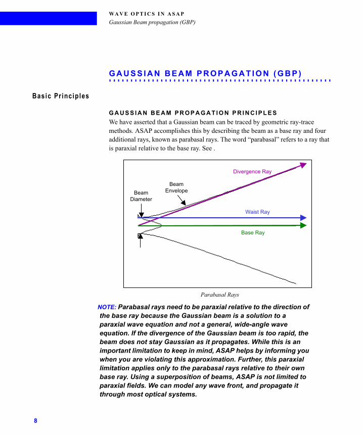
We have asserted that a Gaussian beam can be traced by geometric ray-trace methods. ASAP accomplishes this by describing the beam as a base ray and four additional rays, known as parabasal rays. The word “parabasal” refers to a ray that is paraxial relative to the base ray. See .
Parabasal Rays
NOTE: Parabasal rays need to be paraxial relative to the direction of the base ray because the Gaussian beam is a solution to a paraxial wave equation and not a general, wide-angle wave equation. If the divergence of the Gaussian beam is too rapid, the beam does not stay Gaussian as it propagates. While this is an important limitation to keep in mind, ASAP helps by informing you when you are violating this approximation. Further, this paraxial limitation applies only to the parabasal rays relative to their own base ray. Using a superposition of beams, ASAP is not limited to paraxial fields. We can model any wave front, and propagate it through most optical systems.
Divergence Ray
Waist Ray
Base Ray
BeamEnvelopeBeam
Diameter
8
. . .
. .WA V E O P T I C S I N A S A P
Gaussian Beam propagation (GBP)
The base ray is the main ray associated with the beam. It sits in the center of the beam, as shown in , and points in the direction of beam propagation. It is also the reference ray for the beam. This means that ASAP commands like LIST RAYS and STATS refer to the base rays in your system.
Two of the paraxial rays are waist rays. Only one of these appears in . The other is out of the plane of the paper. The waist rays start parallel to the base ray but are slightly offset. They describe the semidiameter of the beam. Having two waist rays allows us to define a different beam width in two orthogonal axes (that is, an asymmetric beam).
The other two parabasal rays are divergence rays, and their directions define the asymptotic, or far-field, divergence angle of the beam. Once again, two divergence rays are necessary to describe a non-circularly symmetric (that is, elliptically shaped) Gaussian beam, but only the in-plane ray is shown in . The figure also includes the beam envelope, which shows how the beam width expands as the Gaussian beam propagates.
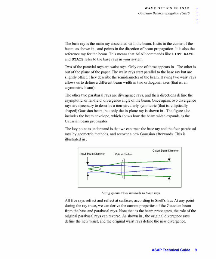
The key point to understand is that we can trace the base ray and the four parabasal rays by geometric methods, and recover a new Gaussian afterwards. This is illustrated in .
Using geometrical methods to trace rays
All five rays refract and reflect at surfaces, according to Snell's law. At any point during the ray trace, we can derive the current properties of the Gaussian beam from the base and parabasal rays. Note that as the beam propagates, the role of the original parabasal rays can reverse. As shown in , the original divergence rays define the new waist, and the original waist rays define the new divergence.
ASAP Technical Guide 9
WA V E O P T I C S I N A S A P
Gaussian Beam propagation (GBP)
G A U S S I A N B E A M S U P E R P O S I T I O N P R I N C I P L E S
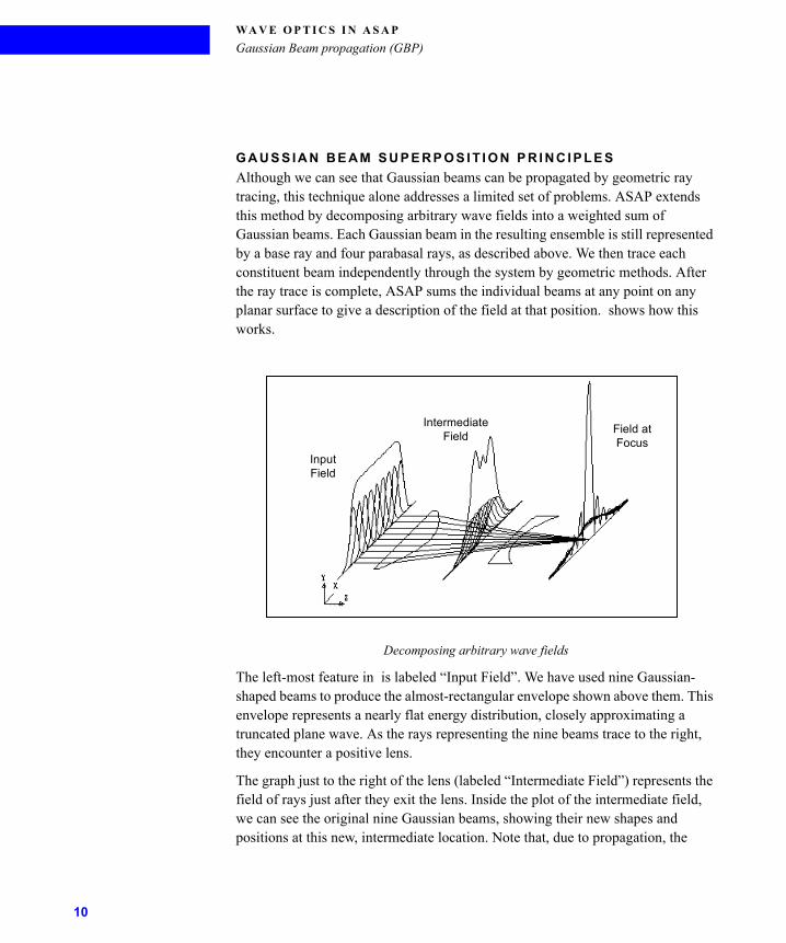
Although we can see that Gaussian beams can be propagated by geometric ray tracing, this technique alone addresses a limited set of problems. ASAP extends this method by decomposing arbitrary wave fields into a weighted sum of Gaussian beams. Each Gaussian beam in the resulting ensemble is still represented by a base ray and four parabasal rays, as described above. We then trace each constituent beam independently through the system by geometric methods. After the ray trace is complete, ASAP sums the individual beams at any point on any planar surface to give a description of the field at that position. shows how this works.
Decomposing arbitrary wave fields
The left-most feature in is labeled “Input Field”. We have used nine Gaussian-shaped beams to produce the almost-rectangular envelope shown above them. This envelope represents a nearly flat energy distribution, closely approximating a truncated plane wave. As the rays representing the nine beams trace to the right, they encounter a positive lens.
The graph just to the right of the lens (labeled “Intermediate Field”) represents the field of rays just after they exit the lens. Inside the plot of the intermediate field, we can see the original nine Gaussian beams, showing their new shapes and positions at this new, intermediate location. Note that, due to propagation, the
InputField
IntermediateField
Field atFocus
10
. . .
. .WA V E O P T I C S I N A S A P
Gaussian Beam propagation (GBP)
individual Gaussian beams now have less height, are wider, and have moved closer together.
Moving further to the right in , the intermediate field propagates through a negative lens before coming to a focus in a plane labeled “Field at Focus”. Note that the individual beams are wider here than when they started out, but all are located at the same position. This makes sense since the lenses produce a far-field-like distribution in the focal plane.
In summary, ASAP is able to propagate energy fields through complex optical systems by decomposing fields into ensembles of Gaussian beams. ASAP then propagates these individual beamlets by geometrical ray-trace methods. This method is discussed in more detail in the sidebar, “Advantages and Limitations of Gaussian Beam Summation” on page 12. For more information about the theoretical foundation of Gaussian beam summation and propagation, see “References—Gaussian Beam” on page 102.
Basic Methods for ASAP Wave Opt icsWhat changes are necessary to take wave optics into account when we use ASAP? Because we are still doing geometrical ray tracing, many of the tools and techniques you may have learned in ASAP still apply. As you work through this technical guide, you will see that
• Everything you have learned about creating geometry and assigning optical properties in ASAP is still valid.
• There are some things to learn about source definition, but much remains familiar.
• Ray tracing is performed in the same ways, but we need to keep a closer watch over the state of our beams as they are traced. Sometimes it is necessary to stop, calculate an intermediate field, and then decompose it into a new set of beams before proceeding through the system.
• New basic analysis tools must be introduced to replace SPOTS and STATS for energy calculations, since these commands work only for geometrical rays.
• The graphical and visualization tools we have been using for geometrical rays still work fine.
ASAP Technical Guide 11
WA V E O P T I C S I N A S A P
Gaussian Beam propagation (GBP)
A D V A N T A G E S A N D L I M I T A T I O N S O F G A U S S I A N B E A M S U M M A T I O N
The Gaussian beam has properties that make it ideal for use in applications such as ASAP. In the paraxial regime, a Gaussian beam maintains its basic form (that is, it stays a Gaussian beam as it propagates), just as a plane or spherical wave does. However, Gaussian beams have properties that make them easier to propagate through optical systems than either plane waves or spherical waves. With plane waves, the wavefront normals propagate with no angular spread, but the plane wave energy extends over all space. With a spherical wave, the energy originates from a single point, but its wavefront normals diverge into an entire sphere. Gaussian beams, on the other hand, have a form that comes close to the spatially localized, non-diverging ideal. The angular divergence of their wavefront normals is the minimum permitted by the wave equation for a given beam width. The energy of the beam is concentrated primarily near its propagation axis, and falls off rapidly with radial position. This allows Gaussian beams to perform localized sampling of optical surfaces. This is important for surfaces with high-order structure. At the same time, these beams stay small as they propagate through an optical system.
Another advantage of Gaussian beam propagation is that, as stated above, the beams can be propagated through an optical system by geometrical ray tracing, which is simple and fast.
The main limitation to the Gaussian beam approach used in ASAP is that it is based on a solution to a scalar wave equation, with the various vector components decoupled. As such, it employs Kirchhoff-type boundary conditions (that is, the field is zero in the geometric shadow of the aperture, and unchanged within the transmitting portion of the aperture). Performing an exact solution to Maxwell's equations, while including the explicit material properties (complex index of refraction) of the aperture, yields a more exact solution. However, these types of solutions are much slower to calculate.
The inherent limitations of scalar methods show up in two important places:
• When aperture dimensions (or object spatial frequencies) are near to, or below, the radiation wavelength, the method tends to break down.
• ASAP can handle polarization effects, but the polarization components (s and p) are treated independently.
On the positive side, ASAP can handle diffraction of rapidly converging or diverging beams (non-paraxial). Although the Gaussian beam is a solution only to a paraxial wave equation, this solution simply means that the divergence of the individual beams (the parabasal rays relative to their base ray) must be paraxial. There is no limitation on the convergence angle of the total field.
12
. . .
. .WA V E O P T I C S I N A S A P
Gaussian Beam propagation (GBP)
We can illustrate many of the basic changes that are needed to start us on a wave-optics problem by writing a brief ASAP script to create a truncated plane wave. This simple script is shown in Example 1.
Example 1 Creating a truncated plane wave
Some of the commands should be familiar. Others may not be, or are at least worthy of additional mention in the context of wave optics.
U N I T S C M
While sometimes neglected in a geometric ray trace, the UNITS command should always be used when we do wave optics. It is used in conjunction with the WAVELENGTH units (see “WAVELENGTH 1 UM” on page 14) to properly scale the beam optical path lengths.
P A R A B A S A L 4
The PARABASAL command sets the number of parabasal rays. In virtually all cases, this value should be set to 4 to obtain the two waist rays and two divergence rays described in the previous section. While there is a PARABASAL 8 setting, it is useful in only a few advanced cases. Using eight parabasal rays slows down ray traces, and can even lead to the masking of some real problems.
ASAP Technical Guide 13
WA V E O P T I C S I N A S A P
Gaussian Beam propagation (GBP)
B E A M S C O H E R E N T D I F F R A C T
Issuing the BEAMS COHERENT DIFFRACT command tells ASAP to operate in the COHERENT mode (see the sidebar, “Wave Optics Terminology”). The COHERENT mode is usually automatically selected when a PARABASAL command is issued; nonetheless, we recommend explicitly issuing a BEAMS COHERENT DIFFRACT command.
W A V E L E N G T H 1 U M
Since the effects of wave optics are wavelength dependent, we must issue a WAVELENGTH command to specify the vacuum wavelength of the source radiation. In addition to the numerical value of the wavelength, we must also explicitly specify the wavelength units (micrometers, in this example). If no units are specified after the numerical value in the WAVELENGTH command, it defaults to system units. To ensure that you get the wavelength units you want, specify the units explicitly in the WAVELENGTH command!
W I D T H S 1 . 6
The WIDTHS parameter controls the amount of overlap between adjoining Gaussian beams. It is not the absolute width of the Gaussian. We will have more to say about exactly what this parameter means when sources are discussed in detail later.
W A V E O P T I C S T E R M I N O L O G Y
If we try to read too much literal meaning into ASAP commands, opportunity for confusion exists. This confusion is particularly true for some of the commands used in wave optics. For example, we turn on wave optics in ASAP with the command BEAMS COHERENT DIFFRACT. The name of this ASAP mode is a little confusing, since when ASAP is placed in this state, it can be used to model systems with any degree of coherence, from incoherent to fully coherent. It also can do more than diffraction. It might be better called “WAVE OPTICS”, since it deals with complex wave functions that are
solutions to the wave equation. Because BEAMS COHERENT DIFFRACT is the command syntax we use within ASAP, the blanket term “coherent” is sometimes used to describe this ASAP mode, even though this is not what we mean in a strict optical sense. So, to avoid confusion, we capitalize COHERENT in this document, whenever it is used to describe the wave-optics mode in ASAP. When “coherent” is used in the optical sense, it is in lower case. Similarly, the ASAP flux calculation command FIELD (see page -21) is capitalized, while the generic “field” is not.
14
. . .
. .WA V E O P T I C S I N A S A P
Gaussian Beam propagation (GBP)
The next two commands define a GRID source directed along the Z-axis. This source type may be familiar from your earlier ASAP work, but now each position in the 21X21 grid is occupied by a Gaussian beam rather than a single ray. The superposition of these beams gives us the truncated plane wave we desire. This and other types of coherent sources are discussed in detail in “COHERENT Sources”, which begins on page -37.
P L O T B E A M S
This command is a graphical option used in COHERENT ASAP beam analysis. The result appears in . Each ring represents the current width of each Gaussian beam that makes up the ensemble. In the figure, we see only the overlap dictated by the WIDTHS command in force when the beams were created. We know from theory, however, that the beams expand as the wave front propagates. We use PLOT BEAMS and other analysis tools at various times during a ray trace to verify that we are still correctly sampling the geometry in our optical system.
Results of PLOT BEAMS graphical option
S P R E A D N O R M A L
The SPREAD NORMAL command is specific to wave optics calculations in ASAP. It is used to calculate flux density, as we have previously done with SPOTS POSITION. Now, however, the coherent sum of the individual beams must be calculated, not just the flux carried by each ray. In practice, this means that the fields (both amplitude and phase) of each of the beams are summed, and that sum is squared to obtain the energy density. ASAP does this calculation at the center of each PIXELS for the current WINDOW.
ASAP Technical Guide 15
WA V E O P T I C S I N A S A P
Gaussian Beam propagation (GBP)
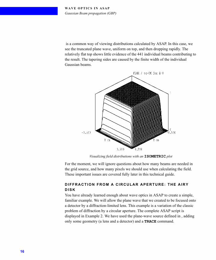
is a common way of viewing distributions calculated by ASAP. In this case, we see the truncated plane wave, uniform on top, and then dropping rapidly. The relatively flat top shows little evidence of the 441 individual beams contributing to the result. The tapering sides are caused by the finite width of the individual Gaussian beams.
Visualizing field distributions with an ISOMETRIC plot
For the moment, we will ignore questions about how many beams are needed in the grid source, and how many pixels we should use when calculating the field. These important issues are covered fully later in this technical guide.
D I F F R A C T I O N F R O M A C I R C U L A R A P E R T U R E : T H E A I R Y
D I S K
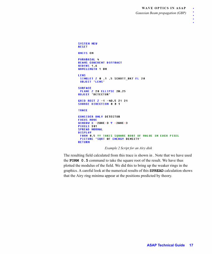
You have already learned enough about wave optics in ASAP to create a simple, familiar example. We will allow the plane wave that we created to be focused onto a detector by a diffraction-limited lens. This example is a variation of the classic problem of diffraction by a circular aperture. The complete ASAP script is displayed in Example 2. We have used the plane-wave source defined in , adding only some geometry (a lens and a detector) and a TRACE command.
16
. . .
. .WA V E O P T I C S I N A S A P
Gaussian Beam propagation (GBP)
Example 2 Script for an Airy disk
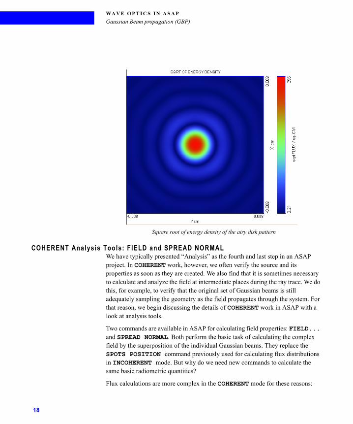
The resulting field calculated from this trace is shown in . Note that we have used the FORM 0.5 command to take the square root of the result. We have thus plotted the modulus of the field. We did this to bring up the weaker rings in the graphics. A careful look at the numerical results of this SPREAD calculation shows that the Airy ring minima appear at the positions predicted by theory.
ASAP Technical Guide 17
WA V E O P T I C S I N A S A P
Gaussian Beam propagation (GBP)
Square root of energy density of the airy disk pattern
COHERENT Analysis Tools: F IELD and SPREAD NORMALWe have typically presented “Analysis” as the fourth and last step in an ASAP project. In COHERENT work, however, we often verify the source and its properties as soon as they are created. We also find that it is sometimes necessary to calculate and analyze the field at intermediate places during the ray trace. We do this, for example, to verify that the original set of Gaussian beams is still adequately sampling the geometry as the field propagates through the system. For that reason, we begin discussing the details of COHERENT work in ASAP with a look at analysis tools.
Two commands are available in ASAP for calculating field properties: FIELD... and SPREAD NORMAL. Both perform the basic task of calculating the complex field by the superposition of the individual Gaussian beams. They replace the SPOTS POSITION command previously used for calculating flux distributions in INCOHERENT mode. But why do we need new commands to calculate the same basic radiometric quantities?
Flux calculations are more complex in the COHERENT mode for these reasons:
18
. . .
. .WA V E O P T I C S I N A S A P
Gaussian Beam propagation (GBP)
In the INCOHERENT mode, each ray is just a point in space, and all its flux is localized within that point. If the ray falls into a particular pixel in the detector plane, that pixel contains that ray’s flux. Other rays in that pixel are added in like drops in a water bucket. The beams in the COHERENT mode, however, have a finite extent. (Technically, Gaussians are infinite, but their region of significance is finite.) The beams can therefore significantly contribute to the field in many of the pixels. Further, to determine the correct flux on an object, it may be necessary to consider beams that narrowly missed that object.
In the INCOHERENT mode, each ray adds its flux to the total flux (that is, 1+1=2). The COHERENT beams, however, must be summed in amplitude and phase, so that two beams with amplitudes of the same magnitude and located at the same position produce different total flux values, depending on their relative phase relationship. For example, they might add destructively to give zero flux, while if they are exactly in phase, four times the flux of each individual beam results.
In the INCOHERENT mode, the flux for all the rays within a given pixel is summed to give the total flux for that pixel. This flux value is the same regardless of how the rays are arranged within that pixel. The result is written to the distribution file, and corresponds to an average flux density for that pixel. In the COHERENT mode, only the flux value at the center of each pixel is calculated. This calculation is done by coherently summing the contributions from all beams at that point. Because ASAP performs the calculation by sampling the field at the center of the pixel, the result carries no information about the flux values elsewhere within that pixel.
As a result of these complexities, the INCOHERENT flux commands (SPOTS, STATS, PATHS, and so on) do not give the correct flux for COHERENT beams. These INCOHERENT commands can still be used to get information about centroid positions and directions, prominent paths, and so on, but the flux values that they give are incorrect.
S P R E A D N O R M A L V E R S U S F I E L D
While SPREAD NORMAL and FIELD can both calculate the energy density of a field, important differences exist between the two commands. The SPREAD NORMAL command calculates only energy density, and generally has only a few optional parameters. The FIELD command is more general, allowing you to calculate many field parameters (like phase or modulus), in addition to energy density. The following usage rules indicate the capabilities of both commands.
ASAP Technical Guide 19
WA V E O P T I C S I N A S A P
Gaussian Beam propagation (GBP)
Use the following commands in their designated situations:
• SPREAD NORMAL to calculate only flux density (flux/area) or irradiance
• FIELD to calculate any of the complex field parameters (see “FIELD” on page 21)
• FIELD when polarization effects must be considered
• SPREAD to sum sources with different wavelengths incoherently (sums energy densities)
• FIELD to sum sources with different wavelengths coherently (sums amplitudes and phases).
The two following sections describe each command in more detail.
S P R E A D N O R M A L
The SPREAD NORMAL command generates an array of real numbers that, as stated previously, corresponds to energy density in the center of each pixel. We can also use it to calculate irradiance (see “IRRADIANCE Command” on page 32).
The most recent WINDOW command defines the area over which the SPREAD calculation is made. The most recent PIXELS command fixes the number of points at which the calculation is performed.
When the SPREAD NORMAL command is used, ASAP coherently sums beams of the same wavelength. Beams with different wavelengths are then incoherently summed.
NOTE: The multiple wavelength behavior of the SPREAD NORMAL command is sometimes exploited to model partial coherence. Since each point in an extended thermal source is spatially incoherent, we can model it as a set of point sources, each with a slightly different wavelength. Down stream, we can correctly calculate the field from that source by using the SPREAD NORMAL command. This method also has application in the modeling of laser-diode arrays.
A glance at the SPREAD command in the ASAP HTML Help reveals alternatives to the NORMAL option. You see DIRECTION, POSITION, and APPROX options, as well. Be careful! As the sidebar, “SPREAD DIRECTION, SPREAD POSITION, and SPREAD APPROX” on page 21, explains, these versions of
20
. . .
. .WA V E O P T I C S I N A S A P
Gaussian Beam propagation (GBP)
SPREAD may not do what you expect. Other SPREAD options, like ADD and DOWN, can be quite useful.
F I E L D
The FIELD command can be issued in seven forms:
In all these cases, the values for the specific form of the command (ENERGY, PHASE, and so on) are stored in an array of real numbers with the file name BRO009.DAT (one real number for each pixel). We can access the values within that real array by issuing a DISPLAY command with no argument following, just as we did after a spot diagram. In addition to this, an array of complex numbers is always created in a file named BRO029.DAT. This complex array contains all the information needed to describe the field. Therefore, if you have already issued any
FIELD AMPLITUDE • Signed modulus of field
FIELD PHASE • Phase of field in radians
FIELD MODULUS • Modulus of the field
FIELD WAVEFRONT • Wavefront of field in waves
FIELD REAL • Real part of field
FIELD IMAGINARY • Imaginary part of field
FIELD ENERGY • Squared modulus of field (energy density)
S P R E A D D I R E C T I O N , S P R E A D P O S I T I O N , A N D S P R E A D A P P R O X
Because SPREAD was introduced for the first time as a COHERENT command, you may think that SPREAD is exclusively for performing wave optics calculations in ASAP. This is not the case. Of the three alternative forms of SPREAD listed here, only SPREAD APPROX is used with COHERENT beams, and only rarely. SPREAD APPROX is used only when astigmatic effects on a beam can be ignored, thus saving computation time.
The other two forms, SPREAD DIRECTION and SPREAD POSITION, are actually INCOHERENT
(geometric ray trace) commands. They are alternatives to SPOTS DIRECTION and SPOTS POSITION, giving the geometric rays a finite extent in space (also known as “fat rays”). This form is sometimes used to “smooth out” distributions, and reduce pixel-to-pixel variations where too few rays were traced to yield good statistics. Such a situation can, of course, lead to misleading visualizations, masking what may be real variations at the noise level. SPREAD DIRECTION and SPREAD POSITION are also rarely used.
ASAP Technical Guide 21
WA V E O P T I C S I N A S A P
Gaussian Beam propagation (GBP)
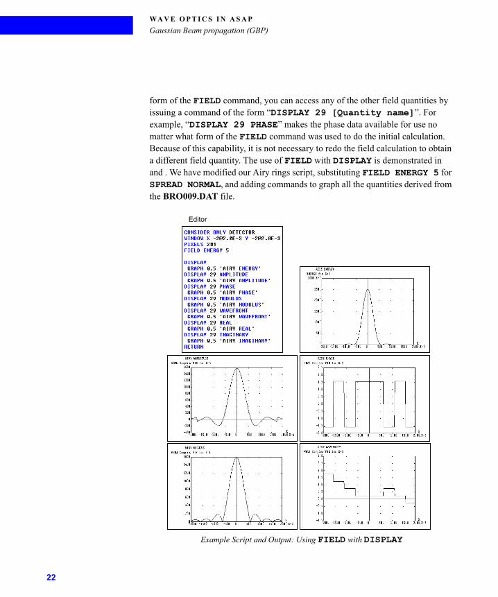
form of the FIELD command, you can access any of the other field quantities by issuing a command of the form “DISPLAY 29 [Quantity name]”. For example, “DISPLAY 29 PHASE” makes the phase data available for use no matter what form of the FIELD command was used to do the initial calculation. Because of this capability, it is not necessary to redo the field calculation to obtain a different field quantity. The use of FIELD with DISPLAY is demonstrated in and . We have modified our Airy rings script, substituting FIELD ENERGY 5 for SPREAD NORMAL, and adding commands to graph all the quantities derived from the BRO009.DAT file.
Example Script and Output: Using FIELD with DISPLAY
Editor
22
. . .
. .WA V E O P T I C S I N A S A P
Gaussian Beam propagation (GBP)
Example Script and Output: Using FIELD with DISPLAY (continued)
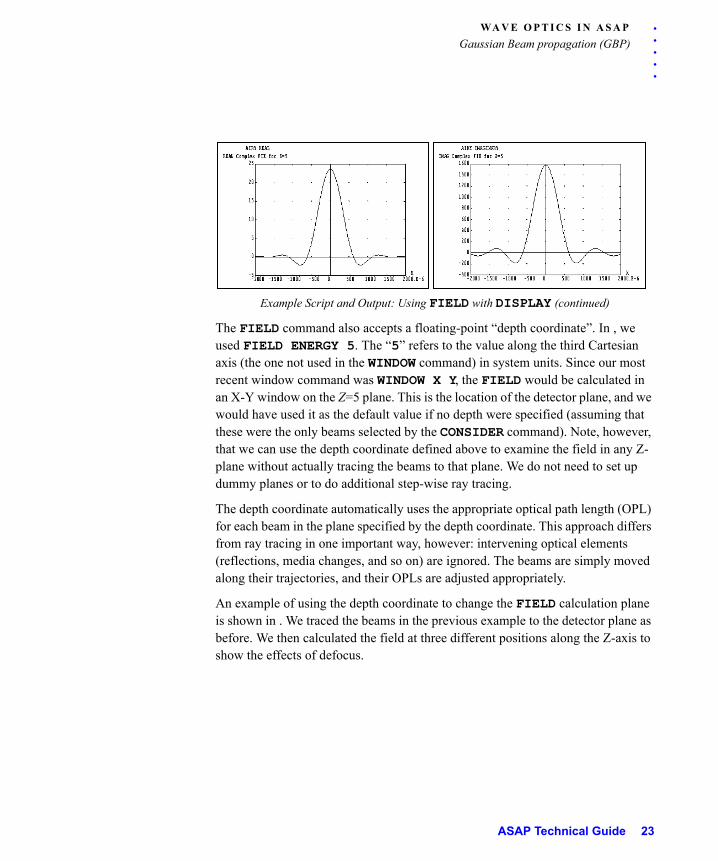
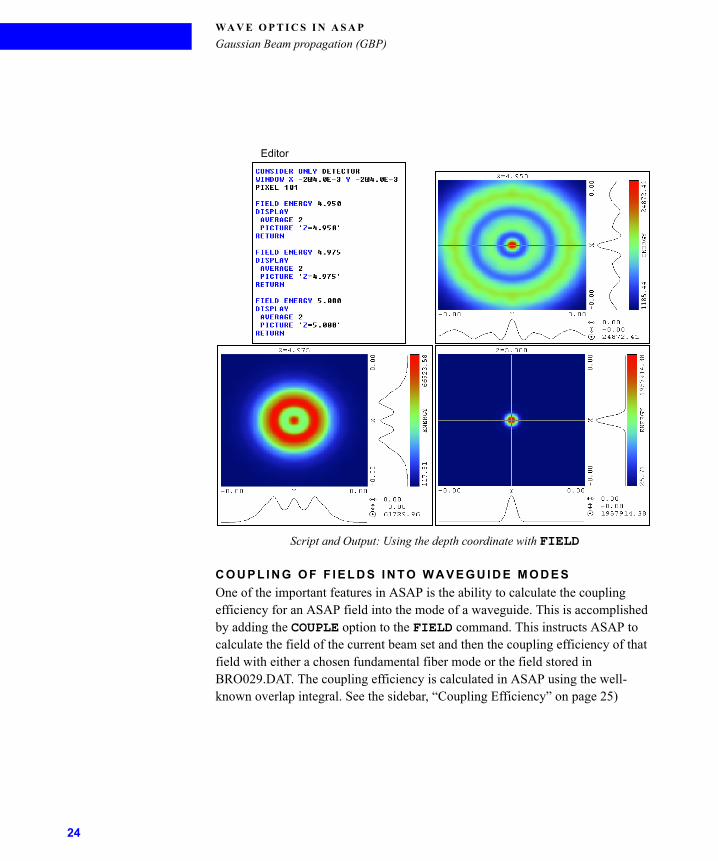
The FIELD command also accepts a floating-point “depth coordinate”. In , we used FIELD ENERGY 5. The “5” refers to the value along the third Cartesian axis (the one not used in the WINDOW command) in system units. Since our most recent window command was WINDOW X Y, the FIELD would be calculated in an X-Y window on the Z=5 plane. This is the location of the detector plane, and we would have used it as the default value if no depth were specified (assuming that these were the only beams selected by the CONSIDER command). Note, however, that we can use the depth coordinate defined above to examine the field in any Z-plane without actually tracing the beams to that plane. We do not need to set up dummy planes or to do additional step-wise ray tracing.
The depth coordinate automatically uses the appropriate optical path length (OPL) for each beam in the plane specified by the depth coordinate. This approach differs from ray tracing in one important way, however: intervening optical elements (reflections, media changes, and so on) are ignored. The beams are simply moved along their trajectories, and their OPLs are adjusted appropriately.
An example of using the depth coordinate to change the FIELD calculation plane is shown in . We traced the beams in the previous example to the detector plane as before. We then calculated the field at three different positions along the Z-axis to show the effects of defocus.
ASAP Technical Guide 23
WA V E O P T I C S I N A S A P
Gaussian Beam propagation (GBP)
Script and Output: Using the depth coordinate with FIELD
C O U P L I N G O F F I E L D S I N T O W A V E G U I D E M O D E S
One of the important features in ASAP is the ability to calculate the coupling efficiency for an ASAP field into the mode of a waveguide. This is accomplished by adding the COUPLE option to the FIELD command. This instructs ASAP to calculate the field of the current beam set and then the coupling efficiency of that field with either a chosen fundamental fiber mode or the field stored in BRO029.DAT. The coupling efficiency is calculated in ASAP using the well-known overlap integral. See the sidebar, “Coupling Efficiency” on page 25)
Editor
24
. . .
. .WA V E O P T I C S I N A S A P
Gaussian Beam propagation (GBP)
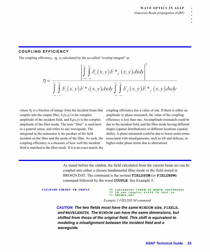
C O U P L I N G E F F I C I E N C Y
The coupling efficiency, , is calculated by the so-called “overlap integral” as
As stated before the sidebar, the field calculated from the current beam set can be coupled into either a chosen fundamental fiber mode or the field stored in BRO029.DAT. The command is the normal FIELDSUM (or FIELDBPM) command followed by the word COUPLE. See Example 3.
Example 3 FIELDSUM command
CAUTION: The two fields must have the same WINDOW size, PIXELS, and WAVELENGTH. The WINDOW can have the same dimensions, but shifted from those of the original field. This shift is equivalent to modeling a misalignment between the incident field and a waveguide.
where is a fraction of energy from the incident beam that couples into the output fiber, Ei(x,y) is the complex amplitude of the incident field, and Ef(x,y) is the complex amplitude of the fiber mode. The term “fiber” is used here in a general sense, and refers to any waveguide. The integrand in the numerator is the product of the field incident on the fiber and the mode of the fiber. As such, the coupling efficiency is a measure of how well the incident field is matched to the fiber mode. If it is an exact match, the
coupling efficiency has a value of one. If there is either an amplitude or phase mismatch, the value of the coupling efficiency is less than one. An amplitude mismatch could be due to the incident field, and the fiber mode having different shapes (spatial distributions) or different locations (spatial shifts). A phase mismatch could be due to lower-order terms associated with misalignments, such as tilt and defocus, or higher-order phase terms due to aberrations.
ASAP Technical Guide 25
WA V E O P T I C S I N A S A P
Gaussian Beam propagation (GBP)
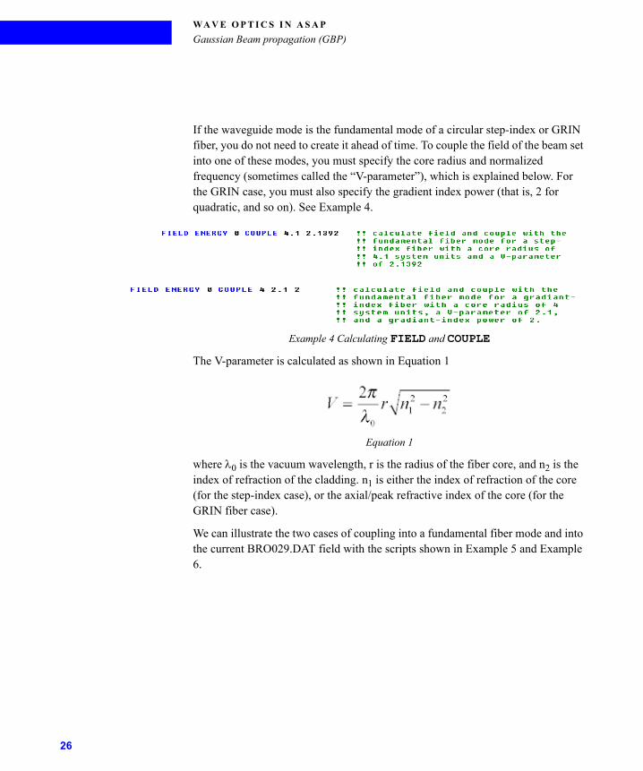
If the waveguide mode is the fundamental mode of a circular step-index or GRIN fiber, you do not need to create it ahead of time. To couple the field of the beam set into one of these modes, you must specify the core radius and normalized frequency (sometimes called the “V-parameter”), which is explained below. For the GRIN case, you must also specify the gradient index power (that is, 2 for quadratic, and so on). See Example 4.
Example 4 Calculating FIELD and COUPLE
The V-parameter is calculated as shown in Equation 1
Equation 1
where 0 is the vacuum wavelength, r is the radius of the fiber core, and n2 is the index of refraction of the cladding. n1 is either the index of refraction of the core (for the step-index case), or the axial/peak refractive index of the core (for the GRIN fiber case).
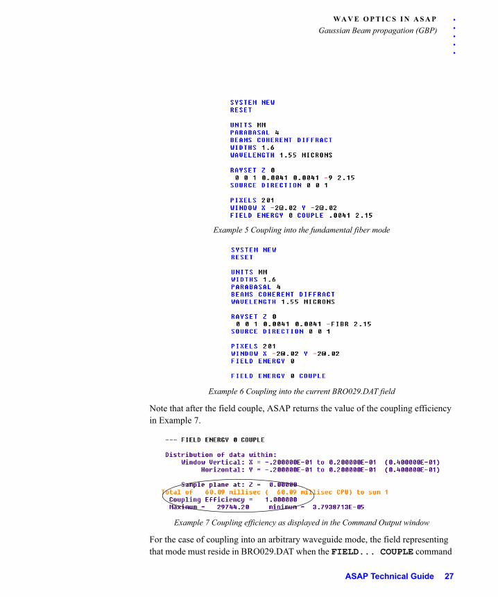
We can illustrate the two cases of coupling into a fundamental fiber mode and into the current BRO029.DAT field with the scripts shown in Example 5 and Example 6.
26
. . .
. .WA V E O P T I C S I N A S A P
Gaussian Beam propagation (GBP)
Example 5 Coupling into the fundamental fiber mode
Example 6 Coupling into the current BRO029.DAT field
Note that after the field couple, ASAP returns the value of the coupling efficiency in Example 7.
Example 7 Coupling efficiency as displayed in the Command Output window
For the case of coupling into an arbitrary waveguide mode, the field representing that mode must reside in BRO029.DAT when the FIELD... COUPLE command
ASAP Technical Guide 27
WA V E O P T I C S I N A S A P
Gaussian Beam propagation (GBP)
is issued. Sometimes, as in Example 5, when you want to calculate the coupling efficiency, the mode of the waveguide is already in BRO029.DAT. Often, a field enters an optical system through a waveguide, and later couples back into an identical output waveguide. If a FIELD was calculated representing the input waveguide mode and no other FIELD was calculated subsequently, then when the beams get to the output waveguide, the field representing the waveguide mode is still in BRO029.DAT. In this case, the FIELD... COUPLE command can be issued and the coupling efficiency obtained.
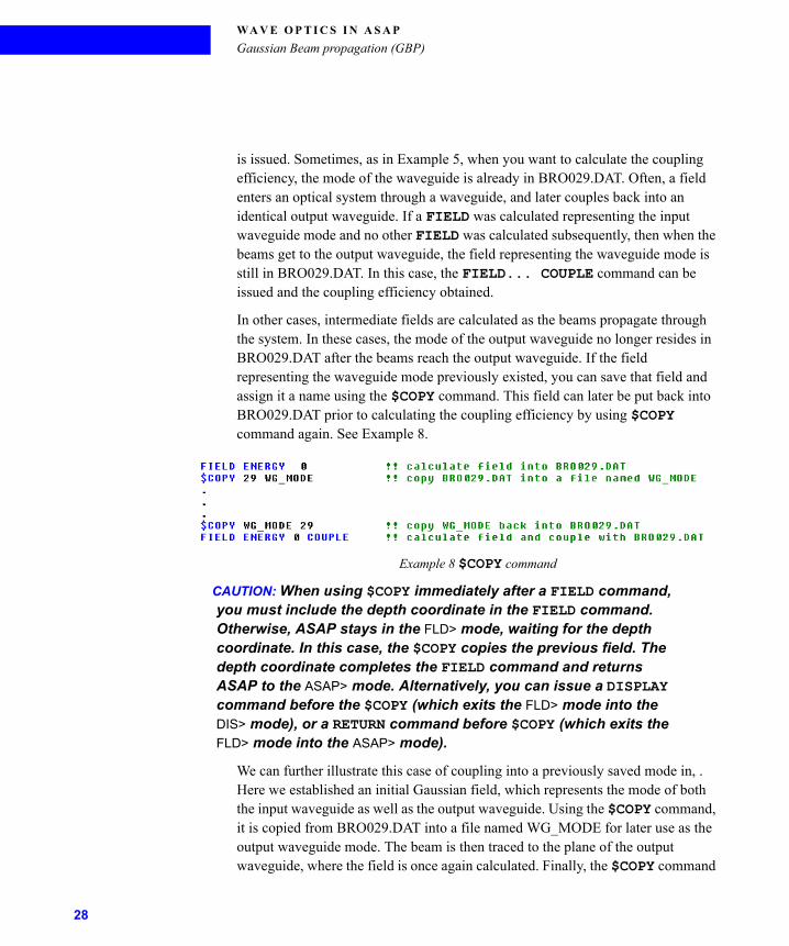
In other cases, intermediate fields are calculated as the beams propagate through the system. In these cases, the mode of the output waveguide no longer resides in BRO029.DAT after the beams reach the output waveguide. If the field representing the waveguide mode previously existed, you can save that field and assign it a name using the $COPY command. This field can later be put back into BRO029.DAT prior to calculating the coupling efficiency by using $COPY command again. See Example 8.
Example 8 $COPY command
CAUTION: When using $COPY immediately after a FIELD command, you must include the depth coordinate in the FIELD command. Otherwise, ASAP stays in the FLD> mode, waiting for the depth coordinate. In this case, the $COPY copies the previous field. The depth coordinate completes the FIELD command and returns ASAP to the ASAP> mode. Alternatively, you can issue a DISPLAY command before the $COPY (which exits the FLD> mode into the DIS> mode), or a RETURN command before $COPY (which exits the FLD> mode into the ASAP> mode).
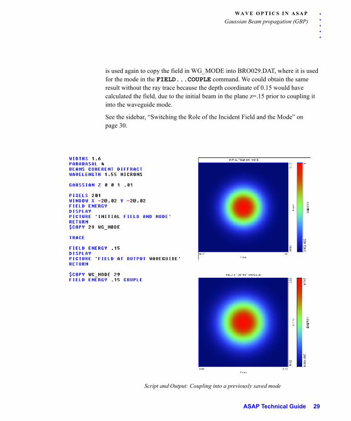
We can further illustrate this case of coupling into a previously saved mode in, . Here we established an initial Gaussian field, which represents the mode of both the input waveguide as well as the output waveguide. Using the $COPY command, it is copied from BRO029.DAT into a file named WG_MODE for later use as the output waveguide mode. The beam is then traced to the plane of the output waveguide, where the field is once again calculated. Finally, the $COPY command
28
. . .
. .WA V E O P T I C S I N A S A P
Gaussian Beam propagation (GBP)
is used again to copy the field in WG_MODE into BRO029.DAT, where it is used for the mode in the FIELD...COUPLE command. We could obtain the same result without the ray trace because the depth coordinate of 0.15 would have calculated the field, due to the initial beam in the plane z=.15 prior to coupling it into the waveguide mode.
See the sidebar, “Switching the Role of the Incident Field and the Mode” on page 30.
Script and Output: Coupling into a previously saved mode
ASAP Technical Guide 29
WA V E O P T I C S I N A S A P
Gaussian Beam propagation (GBP)
S W I T C H I N G T H E R O L E O F T H E I N C I D E N T F I E L D A N D T H E M O D E
C O U P L I N G O F A P O L A R I Z E D F I E L D
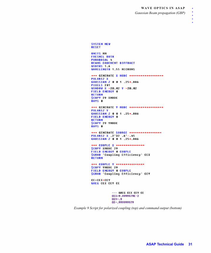
The calculation of coupling efficiency is only slightly more complicated when dealing with polarized fields. If you choose a set of orthogonal polarization modes, such as X, Y, and Z, the total coupling efficiency is the sum of the individual coupling efficiencies. In this case, you must calculate the coupling efficiencies one polarization component at a time, and then sum those efficiencies to obtain the total coupling efficiency. See Example 9.
We can clearly see from inspecting the overlap integral that the role of the incident field and the fiber mode can be reversed without changing the value of the coupling efficiency. Based on this understanding, you may find it convenient to switch the role of the incident field and the mode in ASAP when obtaining the coupling efficiency.
When doing this, you must be careful if you are interested in more than only the value of the coupling efficiency. The FIELD...COUPLE command produces a field in BRO029.DAT, which is the appropriately attenuated field in the form of the mode (the previous BRO029.DAT), not in the form of the incident field.
30
. . .
. .WA V E O P T I C S I N A S A P
Gaussian Beam propagation (GBP)
Example 9 Script for polarized coupling (top) and command output (bottom)
ASAP Technical Guide 31
WA V E O P T I C S I N A S A P
Gaussian Beam propagation (GBP)
C O U P L I N G I N T O M U L T I - M O D E F I B E R
Multi-mode fibers must be treated differently than single-mode fibers. Fibers with core diameters that are hundreds of waves or greater propagate many modes, and are best modeled with geometric ray tracing. For multi-mode fibers with a small number of modes, the calculation of coupling efficiency is more complicated than for either the single-mode or the many mode case. The first step is to calculate the various propagating modes. This step must be done offline, since it cannot be performed within ASAP. Then you must construct each of the modes as ASAP FIELDs, and store them for later coupling. The field to be coupled into the waveguide must be coupled into each mode separately and the sum of those coupling efficiencies gives the total coupling efficiency.
I R R A D I A N C E C O M M A N D
Another fundamental difference between COHERENT and INCOHERENT calculations in ASAP is the additional step required to calculate irradiance, as opposed to energy density. When INCOHERENT rays fall onto a detector plane at an oblique angle, ASAP sums the flux of all the rays in each pixel to determine the total flux in this pixel. This type of "bucket counting" gives the correct irradiance independent of the direction in which the rays are traveling, because groups of rays hitting the detector plane obliquely spread themselves over a larger area.
No such “automatic” correction for angle of incidence effects applies when we trace Gaussian beams. By default, SPREAD NORMAL and FIELD ENERGY calculate a value that is proportional to the energy density of the field in the calculation plane. Both the SPREAD NORMAL and FIELD ENERGY commands can be made to calculate irradiance (which is proportional to the component of the energy density in the direction of the surface normal) by issuing an IRRADIANCE command prior to a FIELD or SPREAD calculation. This command stays active for all subsequent FIELD ENERGY or SPREAD NORMAL commands until an “IRRADIANCE OFF” command is issued.
The IRRADIANCE command works by projecting each beam onto the analysis plane. Ideally, we would like to project the entire field onto the plane. This command is only appropriate for fields where the direction matches the direction of the individual beams. It works well for tilted plane waves, but not for a field at focus.
32
. . .
. .WA V E O P T I C S I N A S A P
Gaussian Beam propagation (GBP)
P R O P A G A T E C O M M A N D
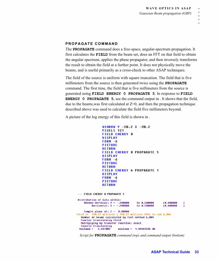
The PROPAGATE command does a free-space, angular-spectrum propagation. It first calculates the FIELD from the beam set, does an FFT on that field to obtain the angular spectrum, applies the phase propagator, and then inversely transforms the result to obtain the field at a further point. It does not physically move the beams, and is useful primarily as a cross-check to other ASAP techniques.
The field of the source is uniform with square truncation. The field that is five millimeters from the source is then generated twice using the PROPAGATE command. The first time, the field that is five millimeters from the source is generated using FIELD ENERGY 0 PROPAGATE 5. In response to FIELD ENERGY 0 PROPAGATE 5, see the command output in . It shows that the field, due to the beams,was first calculated at Z=0, and then the propagation technique described above was used to calculate the field five millimeters beyond.
A picture of the log energy of this field is shown in .
Script for PROPAGATE command (top) and command output (bottom)
ASAP Technical Guide 33
WA V E O P T I C S I N A S A P
Gaussian Beam propagation (GBP)
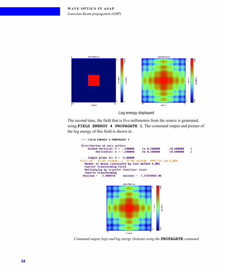
Log energy displayed
The second time, the field that is five millimeters from the source is generated, using FIELD ENERGY 4 PROPAGATE 1. The command output and picture of the log energy of this field is shown in .
Command output (top) and log energy (bottom) using the PROPAGATE command
34
. . .
. .WA V E O P T I C S I N A S A P
Gaussian Beam propagation (GBP)
It shows that the field, due to the beams, was first calculated at Z=4, and then the propagation technique was used to calculate the field one additional millimeter beyond. Both results are nearly identical.The minor differences between the two cases are caused by the differences in the Gaussian beam propagation and the PROPAGATE techniques, and the particular parameters used for each. With some effort to optimize these parameters, these minor differences could be reduced even further. In both cases, the beams still reside at Z=0.
P O L A R I Z A T I O N A N A L Y S I S I N T H E B E A M S C O H E R E N T
D I F F R A C T M O D E
P O L A R I Z A N D T H E F I E L D . . . D E L T A O P T I O N
The FIELD command is used in the COHERENT mode to calculate the complex field, regardless of whether we are examining a scalar field or a vector field including polarization. In the scalar case, ASAP calculates one complex field value per pixel; whereas, in the polarized case, it calculates three complex field values per pixel, one for each of the global X, Y, Z polarization components. Because of this, the maximum number of pixels available in COHERENT polarization analysis goes down by the square root of three in each dimension. The SPREAD NORMAL command can be used to calculate the field energy for COHERENT scalar fields, but it does not account for polarization, and therefore gives incorrect results when used for polarized fields. Use the FIELD ENERGY command to calculate the energy for polarized fields. This command correctly sums the squared moduli of the X, Y, and Z components to obtain the total field energy.
To examine the various field components of the field for a given polarization in ASAP, we must first issue a POLARIZ command, which specifies the component of interest. (A different usage of this command was described earlier to set the polarization state for future source creation.) This step applies for any of the field parameters except FIELD ENERGY, which as stated above, sums all the components together in quadrature.
Example 10 shows the commands we must use to examine the phase of each component after issuing a FIELD command in any form.
POLARIZ XDISPLAY 29 PHASE !! displays x-pol phasePOLARIZ YDISPLAY 29 PHASE !! displays y-pol phasePOLARIZ Z
ASAP Technical Guide 35
WA V E O P T I C S I N A S A P
Gaussian Beam propagation (GBP)
DISPLAY 29 PHASE !! displays z-pol phaseExample 10
The POLARIZ command can also be used to determine the amount of energy in each component. When used in conjunction with the FORM 2 command to square the amplitude (or modulus) values on a pixel-by-pixel basis, we obtain an energy map for a given polarization component. See Example 11.
POLARIZ XDISPLAY 29 AMPLITUDEFORM 2 !! generates array of x-pol energy valuesPOLARIZ YDISPLAY 29 AMPLITUDEFORM 2 !! generates array of y-pol energy valuesPOLARIZ ZDISPLAY 29 AMPLITUDEFORM 2 !! generates array of z-pol energy values
Example 11
The FIELD command used with the DELTA option creates a plot of the polarization ellipses. Unlike the PLOT POLAR command, the plots created by FIELD...DELTA sum the overlapping beam fields with the appropriate relative phases. This process allows for the correct plotting of the polarization ellipses, even after the beams have split into ordinary and extraordinary beams. See .
36

. . .
. .WA V E O P T I C S I N A S A P
Gaussian Beam propagation (GBP)
Example of the same field examined with both the PLOT POLAR command and the FIELD...DELTA command
COHERENT SourcesIn this section, we discuss COHERENT source creation. We look at two source types in some detail:
• the GRID source used for modeling plane or spherical waves
• the GAUSSIAN source for modeling any astigmatic Hermite-Gaussian field.
The RAYSET command can also be used to create COHERENT single-beam sources (See “Using RAYSET command to create the fundamental fiber mode” on page 54.)
An arbitrary source type can be created from field data using the DECOMPOSE command (See “Decomposing Fields” on page 65.)
ASAP Technical Guide 37

WA V E O P T I C S I N A S A P
Gaussian Beam propagation (GBP)
A small, highly divergent source can be made using DECOMPOSE DIRECTION. (See “Creating a small, highly divergent source with DECOMPOSE DIRECTON” on page 97.)
The EMITTING sources (EMITTING RECT, EMITTING OBJECT, and so forth) do not work here. This entire source class, used previously to model extended sources, is not allowed in COHERENT mode.
We address two specific issues common to any COHERENT source that we model when using beam superposition methods:
• What does the WIDTHS command really do, and why is 1.6 usually the correct value?
• How many beams should be used in the ensemble?
G R I D S O U R C E S
The previous sections used examples of the ASAP GRID source as an introduction to COHERENT methods. The exact spacing of the grids, and location of the beams within the grid can have a far more significant impact on a wave-optics analysis than it did in simple geometric ray tracing. This type of information is often critical in determining whether we are sampling the geometry adequately with our ensemble of small beams.
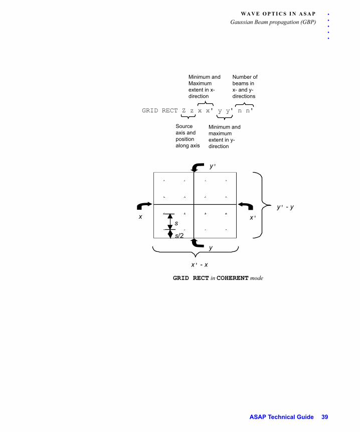
As we have seen, the GRID RECT command, when used in COHERENT mode, creates a truncated plane wave when used in conjunction with SOURCE DIRECTION. GRID creates a rectangular array of beams in a plane, while SOURCE assigns directions to the beams in the grid. The command has exactly the same form as we used for INCOHERENT grids of geometric rays. “GRID RECT in COHERENT mode” shows the basic parameters and their meanings.
38
. . .
. .WA V E O P T I C S I N A S A P
Gaussian Beam propagation (GBP)
GRID RECT in COHERENT mode
GRID RECT Z z x x' y y' n n'
Sourceaxis andpositionalong axis
Minimum andMaximumextent in x-direction
Minimum andmaximumextent in y-direction
Number ofbeams inx- and y-directions
x x'
y
y'
x' - x
y' - y
s
s/2
ASAP Technical Guide 39
WA V E O P T I C S I N A S A P
Gaussian Beam propagation (GBP)
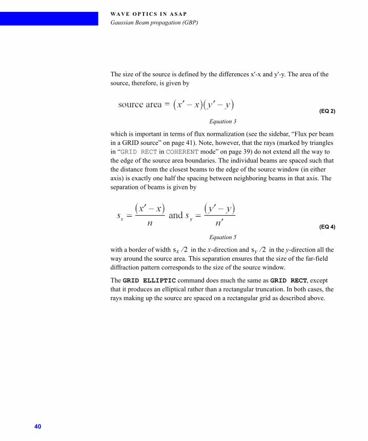
The size of the source is defined by the differences x'-x and y'-y. The area of the source, therefore, is given by
(EQ 2)
Equation 3
which is important in terms of flux normalization (see the sidebar, “Flux per beam in a GRID source” on page 41). Note, however, that the rays (marked by triangles in “GRID RECT in COHERENT mode” on page 39) do not extend all the way to the edge of the source area boundaries. The individual beams are spaced such that the distance from the closest beams to the edge of the source window (in either axis) is exactly one half the spacing between neighboring beams in that axis. The separation of beams is given by
(EQ 4)
Equation 5
with a border of width in the x-direction and in the y-direction all the way around the source area. This separation ensures that the size of the far-field diffraction pattern corresponds to the size of the source window.
The GRID ELLIPTIC command does much the same as GRID RECT, except that it produces an elliptical rather than a rectangular truncation. In both cases, the rays making up the source are spaced on a rectangular grid as described above.
sx 2 sy 2
40
. . .
. .WA V E O P T I C S I N A S A P
Gaussian Beam propagation (GBP)
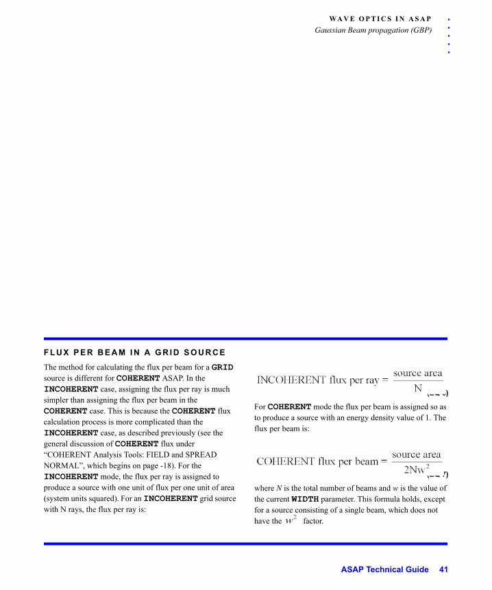
F L U X P E R B E A M I N A G R I D S O U R C E
The method for calculating the flux per beam for a GRID source is different for COHERENT ASAP. In the INCOHERENT case, assigning the flux per ray is much simpler than assigning the flux per beam in the COHERENT case. This is because the COHERENT flux calculation process is more complicated than the INCOHERENT case, as described previously (see the general discussion of COHERENT flux under “COHERENT Analysis Tools: FIELD and SPREAD NORMAL”, which begins on page -18). For the INCOHERENT mode, the flux per ray is assigned to produce a source with one unit of flux per one unit of area (system units squared). For an INCOHERENT grid source with N rays, the flux per ray is:
(EQ 6)
For COHERENT mode the flux per beam is assigned so as to produce a source with an energy density value of 1. The flux per beam is:
(EQ 7)
where N is the total number of beams and w is the value of the current WIDTH parameter. This formula holds, except for a source consisting of a single beam, which does not have the factor.
ASAP Technical Guide 41
WA V E O P T I C S I N A S A P
Gaussian Beam propagation (GBP)
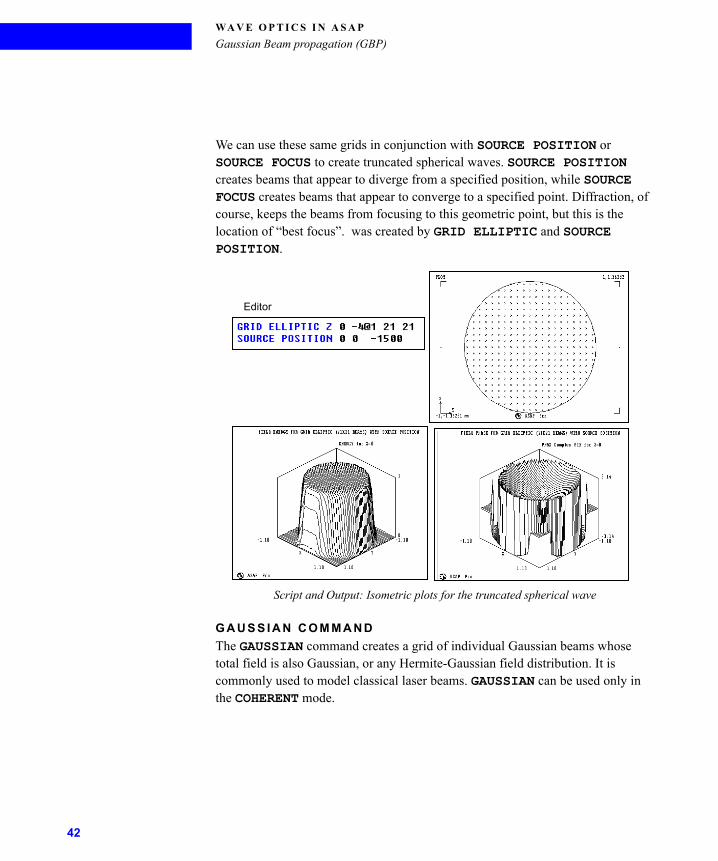
We can use these same grids in conjunction with SOURCE POSITION or SOURCE FOCUS to create truncated spherical waves. SOURCE POSITION creates beams that appear to diverge from a specified position, while SOURCE FOCUS creates beams that appear to converge to a specified point. Diffraction, of course, keeps the beams from focusing to this geometric point, but this is the location of “best focus”. was created by GRID ELLIPTIC and SOURCE POSITION.
Script and Output: Isometric plots for the truncated spherical wave
G A U S S I A N C O M M A N D
The GAUSSIAN command creates a grid of individual Gaussian beams whose total field is also Gaussian, or any Hermite-Gaussian field distribution. It is commonly used to model classical laser beams. GAUSSIAN can be used only in the COHERENT mode.
Editor
42
. . .
. .WA V E O P T I C S I N A S A P
Gaussian Beam propagation (GBP)
Why would it take an ensemble of Gaussian beams to model a Gaussian beam in ASAP? Isn’t one enough? One beam is enough for modeling free-space propagation. However, two types of situations exist for which a single Gaussian beam does not suffice:
1 A Gaussian beam that samples too large a region of a higher-order optical
surface does not remain Gaussian. With more beams, each beam samples a
smaller region, thereby avoiding this problem.
2 Aperture diffraction is involved. As we will see later, a single Gaussian beam
passing through the center of an aperture is oblivious to the shape of the
aperture (see“DECOMPOSE POSITION for sampling apertures”, which begins
on page -72). If the base ray passes, the entire field passes. The effects of the
aperture are apparent when a set of beams with a group distribution that mimics
the shape of the aperture are allowed to propagate from the aperture’s location.
This is only possible if the initial beam is composed of multiple Gaussians.
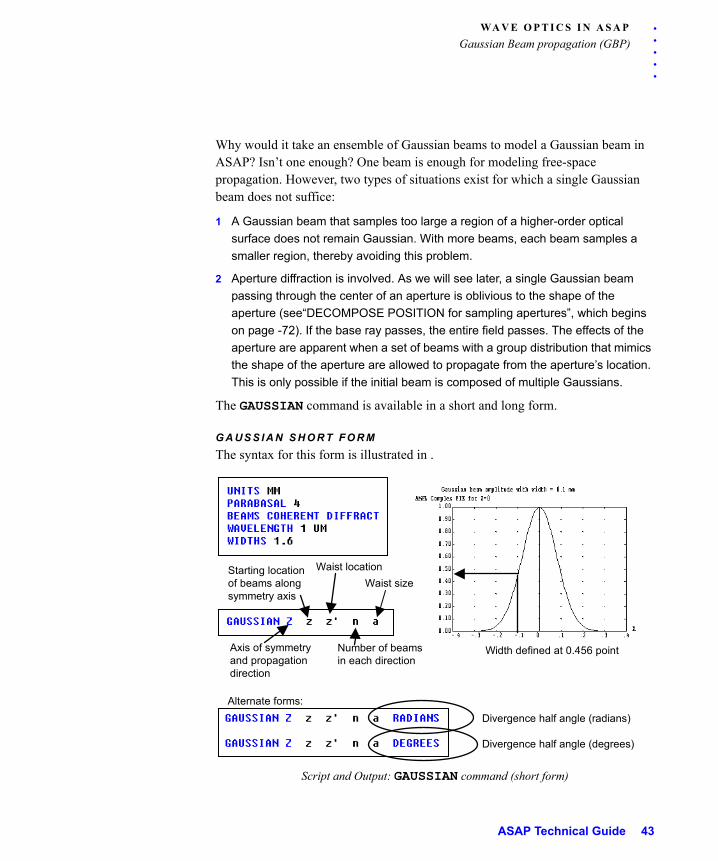
The GAUSSIAN command is available in a short and long form.
G A U S S I A N S H O R T F O R M
The syntax for this form is illustrated in .
Script and Output: GAUSSIAN command (short form)
Width defined at 0.456 pointAxis of symmetryand propagation direction
Starting locationof beams alongsymmetry axis
Waist location
Number of beamsin each direction
Alternate forms:
Divergence half angle (radians)
Divergence half angle (degrees)
Waist size
ASAP Technical Guide 43
WA V E O P T I C S I N A S A P
Gaussian Beam propagation (GBP)
This short form allows the definition of a fundamental mode (0,0) Hermite-Gaussian beam that is radially symmetric and non-astigmatic. We must specify the following parameters:
TABLE 1. Hermite-Gaussian beam parameters
The GAUSSIAN command does not require a SOURCE command to specify beam direction. All the information needed to assign directions to the beams in the ensemble is present in the GAUSSIAN specification.
X, Y, or Z Axis of symmetry of the Gaussian beam. This axis is also the direction of propagation.
x, y, or z Starting location of the beams along the axis of symmetry.
x', y', or z' Location of the beam waist along the axis of symmetry. Just as for SOURCE POSITION and SOURCE FOCUS for GRID sources, beams can be created in any plane, but behave as if they are diverging from or converging toward the specified waist location.
n Number of beams in each axis normal to the axis of symmetry. This is similar to the values specified for GRID ELLIPSE. Since no asymmetry is allowed in the short form of the GAUSSIAN command, the number of rays in each direction must be equal. Therefore, one value is sufficient.
a Either the waist semidiameter, or divergence half angle of the beam. Since these two quantities are related for a Gaussian beam, the specification of one necessarily defines the other. The relationship between waist semidiameter and divergence half angle is as follows:
(EQ 8)
where is the wavelength and is the waist semiwidth in system units. The half angle can be expressed in either degrees or radians, as specified in the Command Input window (see ). Note that this expression for the beam divergence angle is different from that given in many texts. This difference is a result of ASAP using the
point to define the beam waist in amplitude ( for energy) rather than . For more detail, see the sidebar, “ASAP Definition of a Gaussian Beam, Beam Waist, and Divergence” on page 46.
a
e4---–
e2---–
e 2–
44
. . .
. .WA V E O P T I C S I N A S A P
Gaussian Beam propagation (GBP)
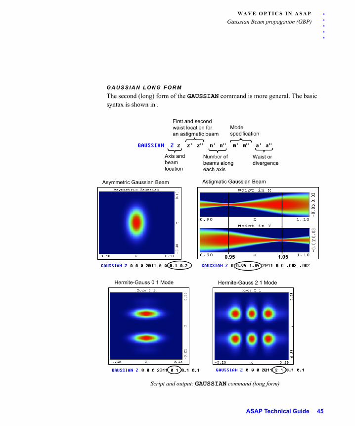
G A U S S I A N L O N G F O R M
The second (long) form of the GAUSSIAN command is more general. The basic syntax is shown in .
Script and output: GAUSSIAN command (long form)
Hermite-Gauss 0 1 Mode Hermite-Gauss 2 1 Mode
Axis andbeamlocation
First and secondwaist location foran astigmatic beam
Modespecification
Waist ordivergence
Number ofbeams alongeach axis
Asymmetric Gaussian Beam Astigmatic Gaussian Beam
0.95 1.05
ASAP Technical Guide 45
WA V E O P T I C S I N A S A P
Gaussian Beam propagation (GBP)
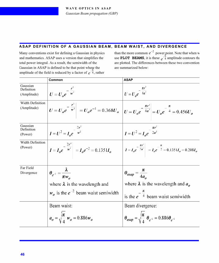
A S A P D E F I N I T I O N O F A G A U S S I A N B E A M , B E A M W A I S T , A N D D I V E R G E N C E
Many conventions exist for defining a Gaussian in physics and mathematics. ASAP uses a version that simplifies the total power integral. As a result, the semiwidth of the Gaussian in ASAP is defined to be that point where the amplitude of the field is reduced by a factor of , rather
than the more common power point. Note that when wuse PLOT BEAMS, it is these amplitude contours thaare plotted. The differences between these two conventionsare summarized below:
e4---–
e 2–
e4---–
Common ASAP
Gaussian Definition(Amplitude)
Width Definition(Amplitude)
Gaussian Definition(Power)
Width Definition(Power)
Far FieldDivergence
46
. . .
. .WA V E O P T I C S I N A S A P
Gaussian Beam propagation (GBP)
The long form offers four additional degrees of freedom:
1 The beam can be astigmatic. If the beam is propagating in the Z-direction, we
can specify two waist locations along Z, one in X, and one in Y.
2 The number of beams in each direction can be specified independently. (We say
more about the best choice for the number of beams in “How many beams?”,
which begins on page -50.)
3 Hermite-Gauss beam modes other than (0,0) can be specified.
4 The beam can be asymmetric. If the beam is propagating in the Z-direction, we
can specify a different beam waist or divergence in the X- and Y-directions.
An astigmatic beam, an asymmetric beam, and two higher-order Hermite-Gauss modes are also illustrated in . Below each beam is the GAUSSIAN command that created it, with the relevant parameters highlighted.
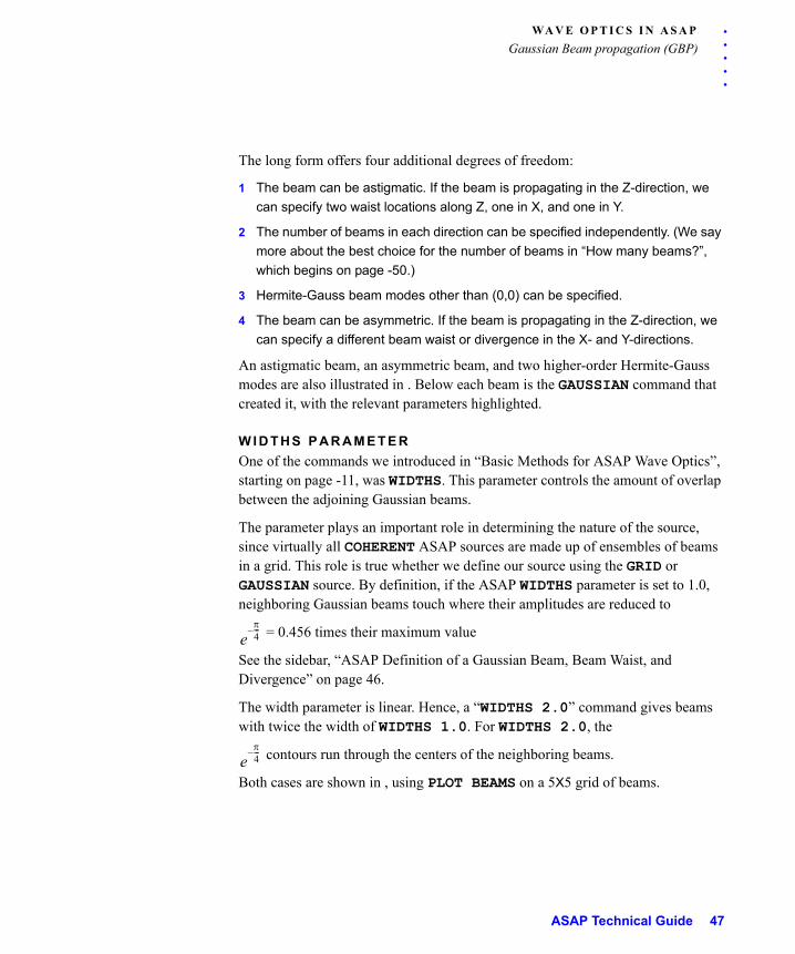
W I D T H S P A R A M E T E R
One of the commands we introduced in “Basic Methods for ASAP Wave Optics”, starting on page -11, was WIDTHS. This parameter controls the amount of overlap between the adjoining Gaussian beams.
The parameter plays an important role in determining the nature of the source, since virtually all COHERENT ASAP sources are made up of ensembles of beams in a grid. This role is true whether we define our source using the GRID or GAUSSIAN source. By definition, if the ASAP WIDTHS parameter is set to 1.0, neighboring Gaussian beams touch where their amplitudes are reduced to
= 0.456 times their maximum value
See the sidebar, “ASAP Definition of a Gaussian Beam, Beam Waist, and Divergence” on page 46.
The width parameter is linear. Hence, a “WIDTHS 2.0” command gives beams with twice the width of WIDTHS 1.0. For WIDTHS 2.0, the
contours run through the centers of the neighboring beams.
Both cases are shown in , using PLOT BEAMS on a 5X5 grid of beams.
e4---–
e4---–
ASAP Technical Guide 47
WA V E O P T I C S I N A S A P
Gaussian Beam propagation (GBP)
WIDTHS parameter
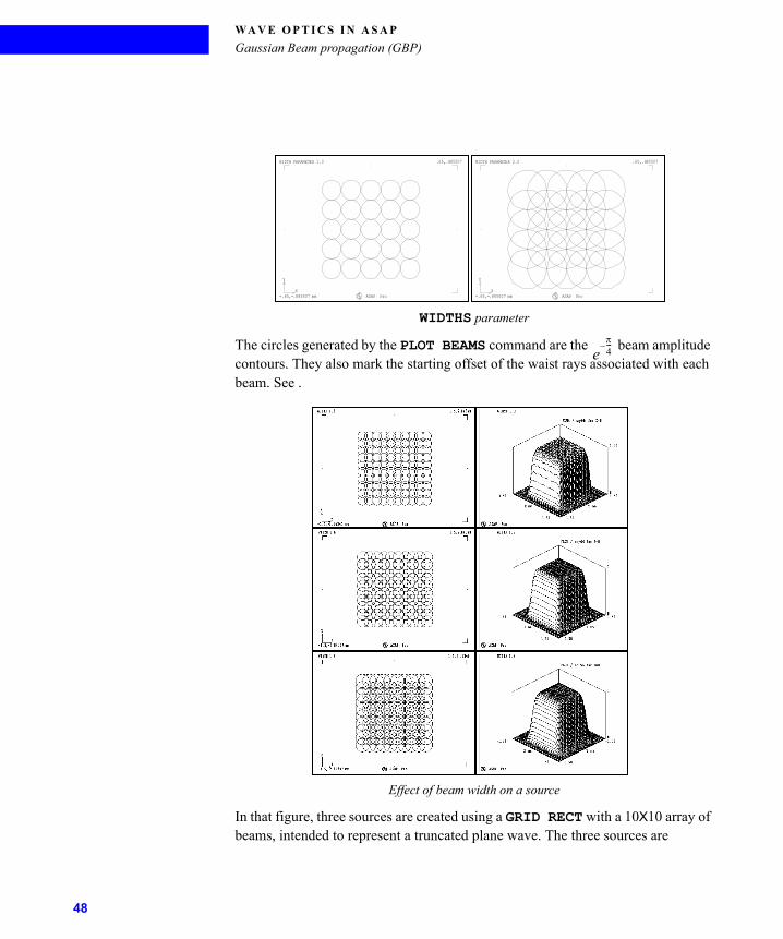
The circles generated by the PLOT BEAMS command are the beam amplitude contours. They also mark the starting offset of the waist rays associated with each beam. See .
Effect of beam width on a source
In that figure, three sources are created using a GRID RECT with a 10X10 array of beams, intended to represent a truncated plane wave. The three sources are
Y
X-.65,-.885507 mm
.65,.885507WIDTH PARAMETER 2.0
ASAP Pro
Y
X-.65,-.885507 mm
.65,.885507WIDTH PARAMETER 1.0
ASAP Pro
e4---–
48
. . .
. .WA V E O P T I C S I N A S A P
Gaussian Beam propagation (GBP)
identical except for the values of their WIDTHS parameters, which are set to 1.3, 1.6, and 1.9.
shows that a source created with a larger WIDTHS parameter has a flatter top (less ripple), but the sides at the truncation edges of the source are not as steep as for the sources with smaller WIDTHS values. We find that in most cases a value of 1.6 represents a fair compromise between these two competing factors. Although some slight ripple is still present, the amplitude of this ripple can be reduced by increasing the number of rays in the ensemble, as discussed in “How many beams?”, which begins on page -50.
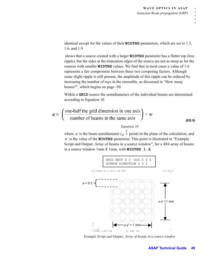
Within a GRID source the semidiameters of the individual beams are determined according to Equation 10
(EQ 9)
Equation 10
where is the beam semidiameter ( point) in the plane of the calculation, and is the value of the WIDTHS parameter. This point is illustrated in “Example
Script and Output: Array of beams in a source window”, for a 4X4 array of beams in a source window 1mm X 1mm, with WIDTHS 1.6.
Example Script and Output: Array of beams in a source window
a e4---–
w
GRID RECT Z 0 [email protected] 4 4SOURCE DIRECTION 0 0 1
y-y' = 1 mm
a = 0.2
x-x' =1 mm
X
Y-.749999,-1.02173 mm
.75,1.021744 X 4 Beams on a 1 mm X 1 mm GRID
ASAP Pro
ASAP Technical Guide 49
WA V E O P T I C S I N A S A P
Gaussian Beam propagation (GBP)
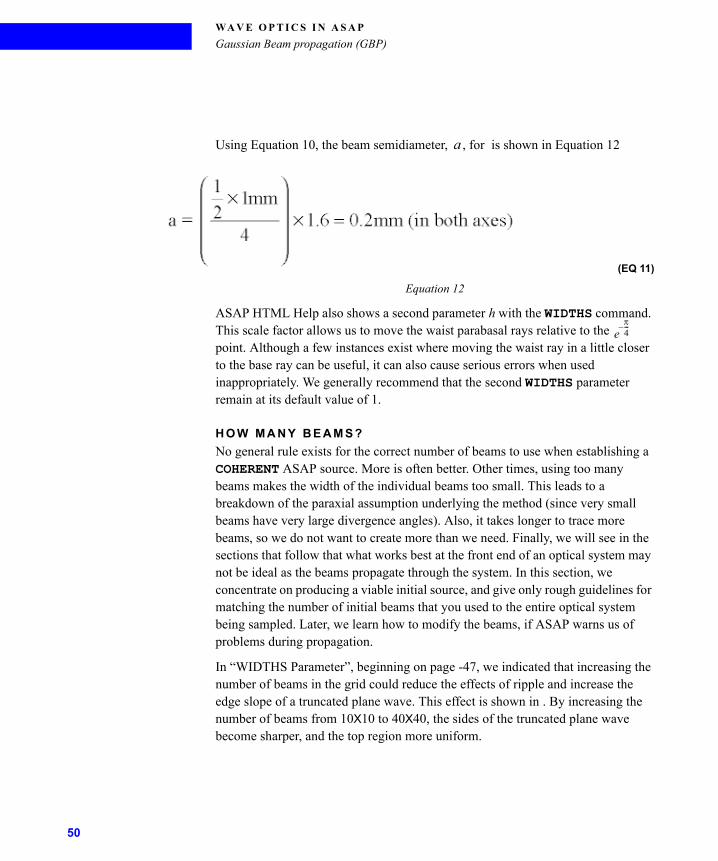
Using Equation 10, the beam semidiameter, , for is shown in Equation 12
(EQ 11)
Equation 12
ASAP HTML Help also shows a second parameter h with the WIDTHS command. This scale factor allows us to move the waist parabasal rays relative to the point. Although a few instances exist where moving the waist ray in a little closer to the base ray can be useful, it can also cause serious errors when used inappropriately. We generally recommend that the second WIDTHS parameter remain at its default value of 1.
H O W M A N Y B E A M S ?
No general rule exists for the correct number of beams to use when establishing a COHERENT ASAP source. More is often better. Other times, using too many beams makes the width of the individual beams too small. This leads to a breakdown of the paraxial assumption underlying the method (since very small beams have very large divergence angles). Also, it takes longer to trace more beams, so we do not want to create more than we need. Finally, we will see in the sections that follow that what works best at the front end of an optical system may not be ideal as the beams propagate through the system. In this section, we concentrate on producing a viable initial source, and give only rough guidelines for matching the number of initial beams that you used to the entire optical system being sampled. Later, we learn how to modify the beams, if ASAP warns us of problems during propagation.
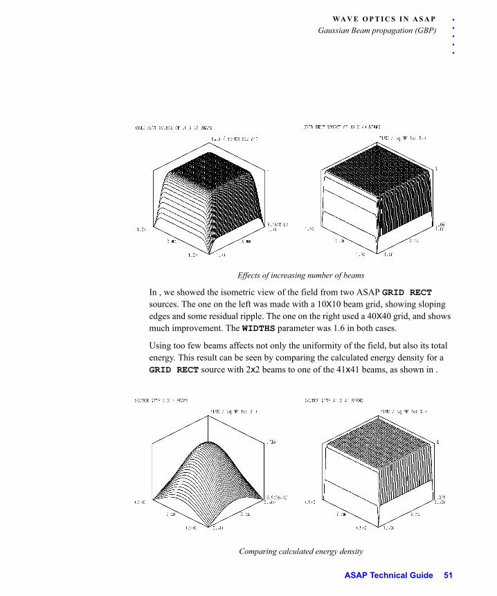
In “WIDTHS Parameter”, beginning on page -47, we indicated that increasing the number of beams in the grid could reduce the effects of ripple and increase the edge slope of a truncated plane wave. This effect is shown in . By increasing the number of beams from 10X10 to 40X40, the sides of the truncated plane wave become sharper, and the top region more uniform.
a
e4---–
50
. . .
. .WA V E O P T I C S I N A S A P
Gaussian Beam propagation (GBP)
Effects of increasing number of beams
In , we showed the isometric view of the field from two ASAP GRID RECT sources. The one on the left was made with a 10X10 beam grid, showing sloping edges and some residual ripple. The one on the right used a 40X40 grid, and shows much improvement. The WIDTHS parameter was 1.6 in both cases.
Using too few beams affects not only the uniformity of the field, but also its total energy. This result can be seen by comparing the calculated energy density for a GRID RECT source with 2x2 beams to one of the 41x41 beams, as shown in .
Comparing calculated energy density
ASAP Technical Guide 51
WA V E O P T I C S I N A S A P
Gaussian Beam propagation (GBP)
Peak energy density is also affected by the number of beams in the grid. The example on the left was made from a 2x2 grid of beams. In addition to being a poor simulation of a truncated plane wave, it falls far short of the unit energy density expected, as achieved by the 41x41 beam grid on the right. Since the source occupies unit area, it should have an energy density of 1 (see sidebar, “Flux per beam in a GRID source” on page 41). From this figure, however, we see that the field generated by 2x2 beams has a maximum energy density value of only 0.716, and is non-uniform. It looks Gaussian (which is not surprising, since it is composed of only four Gaussian beams).
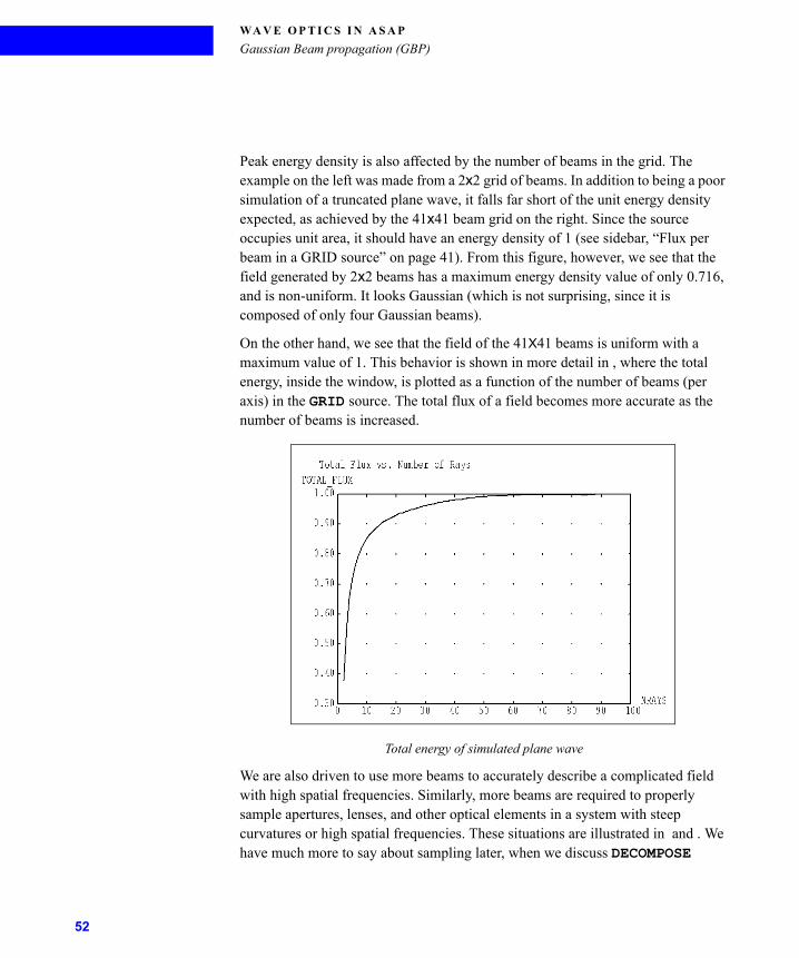
On the other hand, we see that the field of the 41X41 beams is uniform with a maximum value of 1. This behavior is shown in more detail in , where the total energy, inside the window, is plotted as a function of the number of beams (per axis) in the GRID source. The total flux of a field becomes more accurate as the number of beams is increased.
Total energy of simulated plane wave
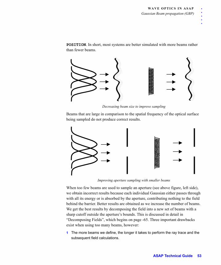
We are also driven to use more beams to accurately describe a complicated field with high spatial frequencies. Similarly, more beams are required to properly sample apertures, lenses, and other optical elements in a system with steep curvatures or high spatial frequencies. These situations are illustrated in and . We have much more to say about sampling later, when we discuss DECOMPOSE
52
. . .
. .WA V E O P T I C S I N A S A P
Gaussian Beam propagation (GBP)
POSITION. In short, most systems are better simulated with more beams rather than fewer beams.
Decreasing beam size to improve sampling
Beams that are large in comparison to the spatial frequency of the optical surface being sampled do not produce correct results.
Improving aperture sampling with smaller beams
When too few beams are used to sample an aperture (see above figure, left side), we obtain incorrect results because each individual Gaussian either passes through with all its energy or is absorbed by the aperture, contributing nothing to the field behind the barrier. Better results are obtained as we increase the number of beams. We get the best results by decomposing the field into a new set of beams with a sharp cutoff outside the aperture’s bounds. This is discussed in detail in “Decomposing Fields”, which begins on page -65. Three important drawbacks exist when using too many beams, however:
1 The more beams we define, the longer it takes to perform the ray trace and the
subsequent field calculations.
ASAP Technical Guide 53
WA V E O P T I C S I N A S A P
Gaussian Beam propagation (GBP)
2 Individual beams making up the ensemble can become too small compared to a
wavelength. As we increase the number of beams in a grid source, the size of
the individual beams necessarily decreases. There is a limit to how small the
beams can become before some of the basic paraxial assumptions are violated.
3 Beams that start small have large divergence angles, and can become too large
later in the process.
The first issue (ray trace and calculation speed) is a familiar problem in Monte Carlo ray-trace applications, where more is better, but sometimes it just takes too long. The second issue (individual beam size) is subtler. ASAP warns us when the beam waists of the individual Gaussians in the ensemble are one wavelength or smaller (see “Warning *** Beam height in waves...” on page 58).
The GAUSSIAN command can help us around this small-beam constraint, under many circumstances. By specifying the start location of the beams far downstream from the waist, we can avoid pinching a large grid of small beams into a very small area. The field is still correct at the waist, but because individual beams were established with sufficient width, they propagate without problems.
NOTE: This technique may not be appropriate if the total Gaussian beam is of the same order as the wavelength of the beam. To create a source to represent small fields of arbitrary shape, use a DECOMPOSE DIRECTION command. This is addressed in “Decomposing Fields”, beginning on page -65.
In summary, the best approach to assigning the number of beams to the source is to use the minimum number necessary to yield a low-ripple wave front with the appropriate total flux. To confirm this, we can perform a SPREAD NORMAL or FIELD ENERGY calculation as soon as the source is created, and make an ISOMETRIC plot of the result to verify the behavior of the source. Other issues arise when we begin moving the beams through the system. It may be necessary, for example, to increase the number of beams so that we accurately sample the optical elements in our system. ASAP issues warnings and error messages at various points during the process if we are getting into trouble. These issues are discussed in the following section.
U S I N G R A Y S E T C O M M A N D T O C R E A T E T H E F U N D A M E N T A L
F I B E R M O D E
One of the more common uses of the RAYSET command in COHERENT ASAP is to create a source that matches the fundamental fiber mode. The amplitude of the
54
. . .
. .WA V E O P T I C S I N A S A P
Gaussian Beam propagation (GBP)
fundamental mode for a step-index fiber is a Bessel function. Although a Gaussian beam is a pretty good approximation to the fundamental fiber mode for many applications, significant differences exist in the two functions, particularly in the low-amplitude tail portions of the functions. For modeling the effects such as fiber crosstalk due to the tail portion of a beam overlapping into a neighboring channel, using the correct fiber mode can be critical. The syntax for the RAYSET command used to create the fundamental fiber mode is shown below.
RAYSET Z z
x y f x' y' k s
The first line of the command syntax contains the source origination plane and its location. The second line has the values for the other two coordinates in the origination plane (x and y), the initial beam flux (f), the two core semi-diameters (x and y), the shape parameter (k), and the normalized frequency s (also called the V-parameter; see “Coupling of fields into waveguide modes” on page 24.) This source is only for circular core fibers, so x must equal y. To signify that the source is COHERENT, the shape parameter must be preceded by a minus sign. For the fundamental fiber mode, the shape parameter can be specified either by its name, -FIBR or its number -9. An example of a fundamental fiber mode source with a core radius of 4.1 system units and a V parameter of 2.135 is shown below. Note that the RAYSET command must be followed by a SOURCE DIRECTION command. See .
Example Script: RAYSET followed by SOURCE DIRECTION command
C R E A T I N G P O L A R I Z E D S O U R C E S
The POLARIZ command must be issued prior to polarized source creation. This command sets the polarization for all future source creation. The polarization state given in the POLARIZ command stays in effect until a different POLARIZ command is issued. The POLARIZ command is also used to examine the properties of the individual X, Y, or Z field components. This second type of application of the POLARIZ command was described previously in this guide in the analysis section (see the section, “POLARIZ and the FIELD ... DELTA option” on page 35).
ASAP Technical Guide 55
WA V E O P T I C S I N A S A P
Gaussian Beam propagation (GBP)
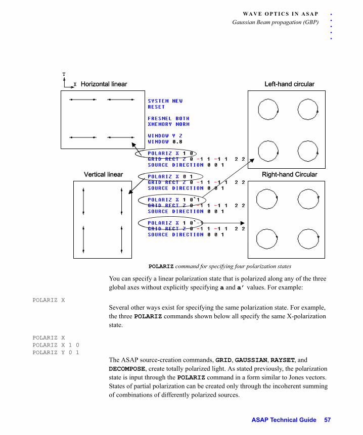
Similar to the common Jones vector representation, the POLARIZ command describes the polarization state of the light by specifying the complex amplitude of two orthogonal polarization states. The ASAP syntax for creating the intended state of polarization is shown in Example 12.
Example 12
The first entry after the word POLARIZ is one of the global X, Y, or Z axes. The value of the a entry specifies the complex amplitude of the polarization component in this specified global axis direction. The a’ term that follows the a term gives the complex amplitude of the polarization component orthogonal to both the a component and the ray direction. ROTATE or SOURCE DIRECTION is applied after ray creation, and gives rise to polarization directions that remain orthogonal to the ray propagation direction. See .
56
. . .
. .WA V E O P T I C S I N A S A P
Gaussian Beam propagation (GBP)
POLARIZ command for specifying four polarization states
You can specify a linear polarization state that is polarized along any of the three global axes without explicitly specifying a and a’ values. For example:
POLARIZ XSeveral other ways exist for specifying the same polarization state. For example, the three POLARIZ commands shown below all specify the same X-polarization state.
POLARIZ XPOLARIZ X 1 0POLARIZ Y 0 1
The ASAP source-creation commands, GRID, GAUSSIAN, RAYSET, and DECOMPOSE, create totally polarized light. As stated previously, the polarization state is input through the POLARIZ command in a form similar to Jones vectors. States of partial polarization can be created only through the incoherent summing of combinations of differently polarized sources.
Horizontal linear
Vertical linear
Left-hand circular
Right-hand Circular
Horizontal linear
Vertical linear
Left-hand circular
Right-hand Circular
ASAP Technical Guide 57
WA V E O P T I C S I N A S A P
Gaussian Beam propagation (GBP)
Warnings and Error Messages
W A R N I N G S A N D E R R O R S I N C O H E R E N T M O D E
In many of the wave optics problems you investigate with ASAP, ray tracing is simple and straightforward. As in our Airy disk example, the beams proceed through the system without difficulty and produce an accurate result. In other cases, however, ASAP issues warning or error messages, letting you know that you have violated the basic assumptions of the method. Warnings and errors messages can appear at various times, including
• when the source is created,
• during a ray trace, and
• during the field calculation.
These messages seldom mean that you must abandon the effort. In most cases, a solution exists. It only remains to understand the source of the error, and take corrective action before proceeding with the analysis.
E R R O R S W H E N A S O U R C E I S C R E A T E D
Warning *** Beam height in waves...
This error occurs as soon as ASAP attempts to create the rays in a new source. The error is issued when the individual Gaussian beams are getting too small. Try creating a 17X17 grid in a space only 0.02X0.02 mm on each side with a 1 m wavelength:
WAVELENGTH 1 UM
WIDTH 1.6
GRID RECT Z 0 [email protected] 17 17
SOURCE DIRECTION 0 0 1
As soon as the source is created, you see this warning in the Command Output window:
--- GRID RECT Z 0 [email protected] 17 17
Warning *** Beam height in waves = .9411765
58
. . .
. .WA V E O P T I C S I N A S A P
Gaussian Beam propagation (GBP)
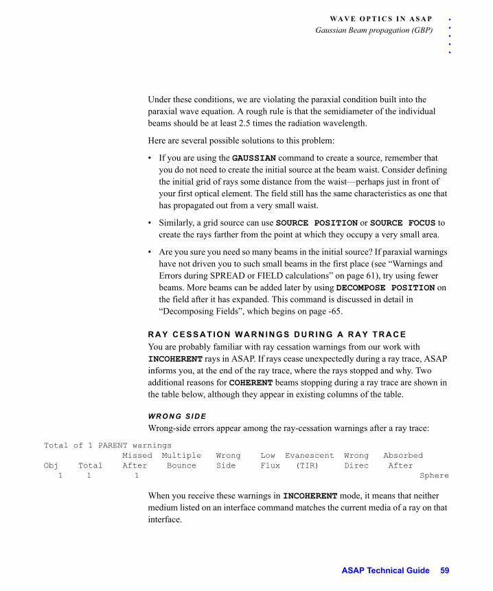
Under these conditions, we are violating the paraxial condition built into the paraxial wave equation. A rough rule is that the semidiameter of the individual beams should be at least 2.5 times the radiation wavelength.
Here are several possible solutions to this problem:
• If you are using the GAUSSIAN command to create a source, remember that you do not need to create the initial source at the beam waist. Consider defining the initial grid of rays some distance from the waist—perhaps just in front of your first optical element. The field still has the same characteristics as one that has propagated out from a very small waist.
• Similarly, a grid source can use SOURCE POSITION or SOURCE FOCUS to create the rays farther from the point at which they occupy a very small area.
• Are you sure you need so many beams in the initial source? If paraxial warnings have not driven you to such small beams in the first place (see “Warnings and Errors during SPREAD or FIELD calculations” on page 61), try using fewer beams. More beams can be added later by using DECOMPOSE POSITION on the field after it has expanded. This command is discussed in detail in “Decomposing Fields”, which begins on page -65.
R A Y C E S S A T I O N W A R N I N G S D U R I N G A R A Y T R A C E
You are probably familiar with ray cessation warnings from our work with INCOHERENT rays in ASAP. If rays cease unexpectedly during a ray trace, ASAP informs you, at the end of the ray trace, where the rays stopped and why. Two additional reasons for COHERENT beams stopping during a ray trace are shown in the table below, although they appear in existing columns of the table.
WR O N G S I D E
Wrong-side errors appear among the ray-cessation warnings after a ray trace:
Total of 1 PARENT warnings Missed Multiple Wrong Low Evanescent Wrong AbsorbedObj Total After Bounce Side Flux (TIR) Direc After 1 1 1 Sphere
When you receive these warnings in INCOHERENT mode, it means that neither medium listed on an interface command matches the current media of a ray on that interface.
ASAP Technical Guide 59
WA V E O P T I C S I N A S A P
Gaussian Beam propagation (GBP)
In COHERENT mode, wrong-side cessation warnings can have an additional meaning. When a base ray and one or more of its associated parabasal rays become too widely separated, they may take radically different paths through an optical element. ASAP makes sure that the parabasal rays interact with the same surfaces in the same order as the base ray. The program ignores surfaces, reverses parabasal ray directions, and even mathematically extends a surface beyond its stated boundaries to make sure the parabasal rays interact with the same surfaces in the same order as their associated base rays. Sometimes, however, the logic becomes too convoluted, and ASAP cannot resolve the problems. When the base ray and one of its parabasal rays appear to have reached a surface from the opposing direction, ASAP issues the wrong-side error.
When you see a wrong-side error, the cause may be a surface in your system with a large range of surface normals (like a spherical “ball” lens), or adjacent optical elements with different surface normals (like the planes of a corner cube). To eliminate, or at least reduce, the number of wrong-side errors, you generally need to move the parabasal rays closer to the base ray before tracing through the problem surface. You may be able to accomplish this with more beams in the initial source. If the initial beams have diverged considerably since the ray trace began, however, this will likely make the situation worse. The better solution in this case is to use DECOMPOSE POSITION to create new beams just in front of the problem surface.
Another possible solution involves a second, optional parameter on the WIDTH command. We explained that the parabasal rays for a given Gaussian beam start at the 0.456 amplitude point. The second WIDTH parameter allows us to create the parabasal rays at higher amplitude points, closer to the base ray. After tracing, when performing the field calculation, the widths of the Gaussians are readjusted to correct values.
CAUTION: In general, we do not recommend moving the parabasal rays too close to the base ray. The individual Gaussian beams do not sample the surface as effectively, and you may mask other warnings and errors. This parameter does, sometimes, let us work a little closer to the “corners” in a tight space, however.
E V A N E S C E N T ( T I R )
The totally internally reflected (TIR) ray cessation warning appears after the ray trace, to indicate that one or more rays have stopped on a specific surface. When we used INCOHERENT sources, a ray stopped because it was totally internally
60
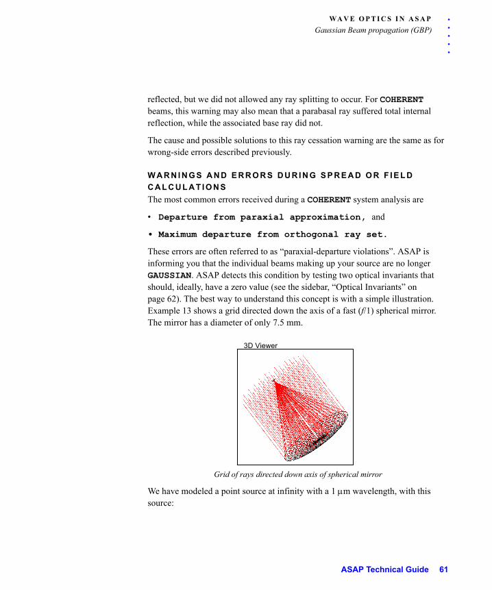
. . .
. .WA V E O P T I C S I N A S A P
Gaussian Beam propagation (GBP)
reflected, but we did not allowed any ray splitting to occur. For COHERENT beams, this warning may also mean that a parabasal ray suffered total internal reflection, while the associated base ray did not.
The cause and possible solutions to this ray cessation warning are the same as for wrong-side errors described previously.
W A R N I N G S A N D E R R O R S D U R I N G S P R E A D O R F I E L D
C A L C U L A T I O N S
The most common errors received during a COHERENT system analysis are
• Departure from paraxial approximation, and
• Maximum departure from orthogonal ray set.
These errors are often referred to as “paraxial-departure violations”. ASAP is informing you that the individual beams making up your source are no longer GAUSSIAN. ASAP detects this condition by testing two optical invariants that should, ideally, have a zero value (see the sidebar, “Optical Invariants” on page 62). The best way to understand this concept is with a simple illustration. Example 13 shows a grid directed down the axis of a fast (f/1) spherical mirror. The mirror has a diameter of only 7.5 mm.
Grid of rays directed down axis of spherical mirror
We have modeled a point source at infinity with a 1 m wavelength, with this source:
3D Viewer
ASAP Technical Guide 61
WA V E O P T I C S I N A S A P
Gaussian Beam propagation (GBP)
O P T I C A L I N V A R I A N T S
Gaussian beams are quadratic in phase. When a beam with quadratic phase intersects an optical component, the effect on the subsequent field phase is approximately an arithmetic sum of the phase terms of the incident field, and the phase term introduced by the optic. Consequently, when a Gaussian beam interacts with an optic that has higher than second-order phase terms, the subsequent phase of the field after the optic also contains higher-order terms. The field is no longer strictly Gaussian.
Small errors can, of course, be tolerated. Otherwise the only optical elements suitable for this type of analysis would be planes and parabolic surfaces intersected on axis. Other surfaces, when expanded in a power series, have higher-order terms. As we note in the main text, the solution to this problem is to make sure that each Gaussian samples a small enough area of an optical element to remain locally quadratic to within an acceptable level of accuracy.
To help us evaluate the departure from quadratic phase, ASAP tests several invariants every time we run SPREAD
NORMAL or FIELD. This test is done on a ray-by-ray basis. The warnings that ASAP sends to the Command Output window have the following specific meanings:
• Departure from paraxial approximation
The complex paraxial optical invariant should be equal to zero, if the parabasal rays remain in a linear region about the base ray. As it sometimes happens for a variety of reasons, the parabasal rays begin to diverge and are no longer linear. This message is printed whenever the complex paraxial invariant exceeds a prescribed value (0.1 waves is the default).
• Max departure from orthogonal ray set
In addition to the complex paraxial optical invariant, several orthogonal invariants should also be equal to zero, if the parabasal rays remain in a linear region about the base ray. This message is printed whenever any of these invariants exceeds a prescribed value (0.1 waves is the default).
62
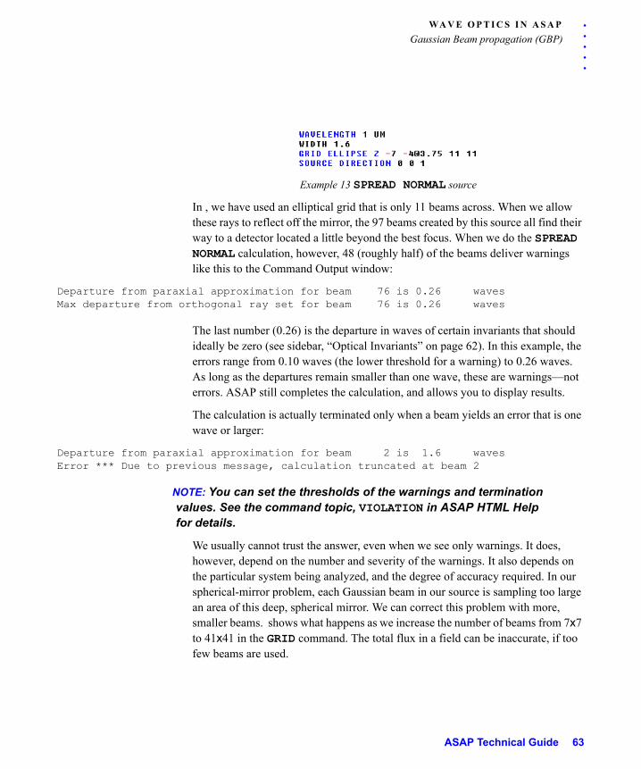
. . .
. .WA V E O P T I C S I N A S A P
Gaussian Beam propagation (GBP)
Example 13 SPREAD NORMAL source
In , we have used an elliptical grid that is only 11 beams across. When we allow these rays to reflect off the mirror, the 97 beams created by this source all find their way to a detector located a little beyond the best focus. When we do the SPREAD NORMAL calculation, however, 48 (roughly half) of the beams deliver warnings like this to the Command Output window:
Departure from paraxial approximation for beam 76 is 0.26 wavesMax departure from orthogonal ray set for beam 76 is 0.26 waves
The last number (0.26) is the departure in waves of certain invariants that should ideally be zero (see sidebar, “Optical Invariants” on page 62). In this example, the errors range from 0.10 waves (the lower threshold for a warning) to 0.26 waves. As long as the departures remain smaller than one wave, these are warnings—not errors. ASAP still completes the calculation, and allows you to display results.
The calculation is actually terminated only when a beam yields an error that is one wave or larger:
Departure from paraxial approximation for beam 2 is 1.6 wavesError *** Due to previous message, calculation truncated at beam 2
NOTE: You can set the thresholds of the warnings and termination values. See the command topic, VIOLATION in ASAP HTML Help for details.
We usually cannot trust the answer, even when we see only warnings. It does, however, depend on the number and severity of the warnings. It also depends on the particular system being analyzed, and the degree of accuracy required. In our spherical-mirror problem, each Gaussian beam in our source is sampling too large an area of this deep, spherical mirror. We can correct this problem with more, smaller beams. shows what happens as we increase the number of beams from 7x7 to 41x41 in the GRID command. The total flux in a field can be inaccurate, if too few beams are used.
ASAP Technical Guide 63
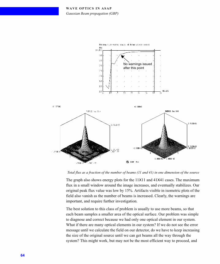
WA V E O P T I C S I N A S A P
Gaussian Beam propagation (GBP)
Total flux as a fraction of the number of beams (11 and 41) in one dimension of the source
The graph also shows energy plots for the 11X11 and 41X41 cases. The maximum flux in a small window around the image increases, and eventually stabilizes. Our original peak flux value was low by 15%. Artifacts visible in isometric plots of the field also vanish as the number of beams is increased. Clearly, the warnings are important, and require further investigation.
The best solution to this class of problem is usually to use more beams, so that each beam samples a smaller area of the optical surface. Our problem was simple to diagnose and correct because we had only one optical element in our system. What if there are many optical elements in our system? If we do not see the error message until we calculate the field on our detector, do we have to keep increasing the size of the original source until we can get beams all the way through the system? This might work, but may not be the most efficient way to proceed, and
No warnings issuedafter this point
64
. . .
. .WA V E O P T I C S I N A S A P
Gaussian Beam propagation (GBP)
sometimes it is not possible. The DECOMPOSE command, which is discussed in the next section, offers a better solution in many cases. If you can identify one or more components that need more beams, you can decompose the field into a new set of smaller beams, just prior to tracing through the troublesome components.
NOTE: Although improper sampling of the optic during the ray trace created the problem, we are not warned of this class of problem until the next FIELD or SPREAD calculation. The optical invariant tests are performed only at this time.
P O S I T I V I T Y V I O L A T I O N S
Like the parabasal departures discussed above, the positivity violation warnings and errors are issued during a SPREAD NORMAL or FIELD ENERGY calculation. The energy density of any Gaussian beam should get smaller as a function of radial distance from the base ray. Situations exist, however, where field calculations that are performed on a specific beam yield energy density values that increase with radial distance from the base ray. This beam is clearly not Gaussian, anymore. Positivity violations always cause calculations to terminate.
The cause of this error is much the same as paraxial or orthogonality departures—interaction with one or more surfaces has violated the basic assumptions of the method. The solutions are also the same as those described for the parabasal departures.
Decomposing Fie ldsDECOMPOSE allows us to create a new set of individual beams that represent the same field as the original beams. Most often, we perform a DECOMPOSE when the existing beamlets are not appropriate to sample an optic or an aperture correctly. Other applications of DECOMPOSE include:
• Creating sources from arbitrary field data,
• Creating highly divergent sources, and
• Obtaining correct FRESNEL transmission and reflection coefficients.
The two forms of the DECOMPOSE command are:
• DECOMPOSE POSITION and
• DECOMPOSE DIRECTION.
ASAP Technical Guide 65
WA V E O P T I C S I N A S A P
Gaussian Beam propagation (GBP)
DECOMPOSE POSITION is the easier of the two to use and understand. Use it whenever the optical surface or aperture you are sampling is large enough to be appropriately sampled with a set of beams, each of whose semidiameters are two to three times the radiation wavelength or greater. We use DECOMPOSE DIRECTION only when the field occupies too small an area to allow us to use DECOMPOSE POSITION.
D E C O M P O S E P O S I T I O N F O R U N D E R - S A M P L E D S U R F A C E S
Use the DECOMPOSE POSITION command when you need to create a new set of beamlets part way through a ray trace to appropriately sample an element of the system geometry. This command creates one new beam in the center of each pixel of the most recent FIELD. The two classes of a problem where appropriate sampling is an issue are:
1 Beams that need to sample a small enough portion (a "locally quadratic" region)
of optical components so that they remain Gaussian, as discussed in “Warnings
and Error Messages”, starting on page -58, and in the sidebar, “Optical
Invariants” on page 62.
2 Our occasional need to “clip” a field, so that it has the appropriate boundaries
after passing through an aperture. DECOMPOSE POSITION is also the correct
command in this case, provided the aperture is not too small. (See
“DECOMPOSE DIRECTION for very small fields” on page 89, for a discussion of
very small apertures.)
We begin with the simple problem of showing how to deal with the “locally quadratic” issues, since we already have some experience with that from the spherical mirror example. shows a set of beams passing through a relatively fast lens and converging on a detector plane.
66
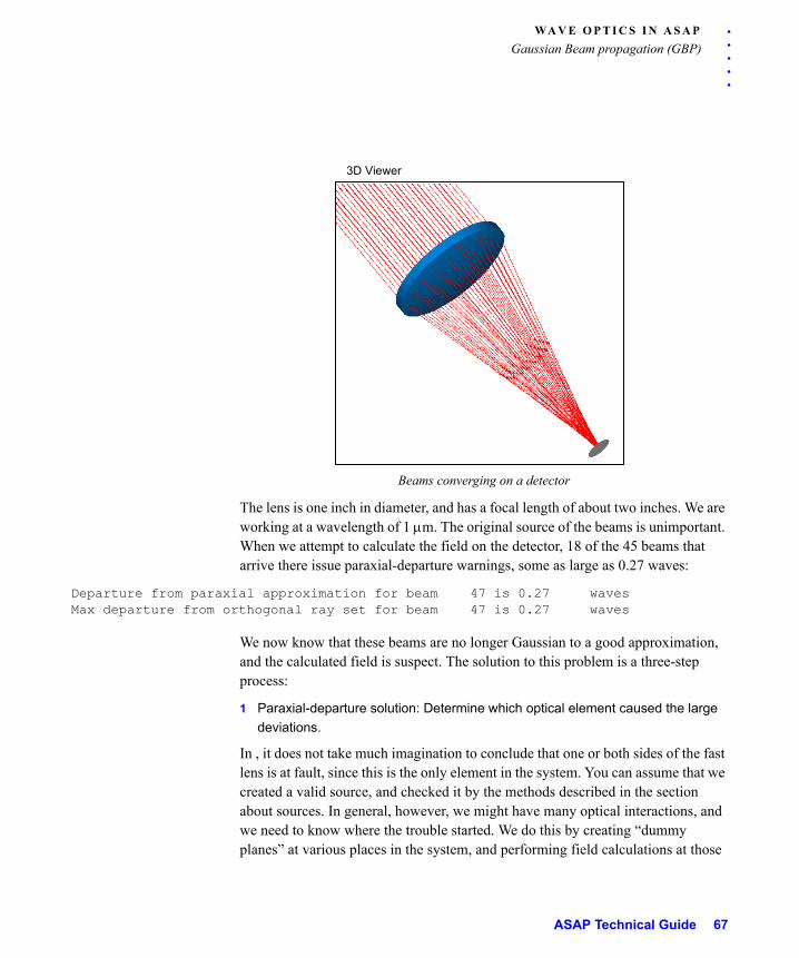
. . .
. .WA V E O P T I C S I N A S A P
Gaussian Beam propagation (GBP)
Beams converging on a detector
The lens is one inch in diameter, and has a focal length of about two inches. We are working at a wavelength of 1 m. The original source of the beams is unimportant. When we attempt to calculate the field on the detector, 18 of the 45 beams that arrive there issue paraxial-departure warnings, some as large as 0.27 waves:
Departure from paraxial approximation for beam 47 is 0.27 wavesMax departure from orthogonal ray set for beam 47 is 0.27 waves
We now know that these beams are no longer Gaussian to a good approximation, and the calculated field is suspect. The solution to this problem is a three-step process:
1 Paraxial-departure solution: Determine which optical element caused the large
deviations.
In , it does not take much imagination to conclude that one or both sides of the fast lens is at fault, since this is the only element in the system. You can assume that we created a valid source, and checked it by the methods described in the section about sources. In general, however, we might have many optical interactions, and we need to know where the trouble started. We do this by creating “dummy planes” at various places in the system, and performing field calculations at those
3D Viewer
ASAP Technical Guide 67
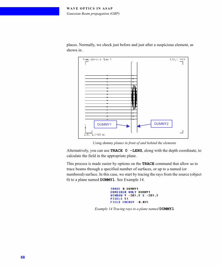
WA V E O P T I C S I N A S A P
Gaussian Beam propagation (GBP)
places. Normally, we check just before and just after a suspicious element, as shown in .
Using dummy planes in front of and behind the elements
Alternatively, you can use TRACE 0 -LENS, along with the depth coordinate, to calculate the field in the appropriate plane.
This process is made easier by options on the TRACE command that allow us to trace beams through a specified number of surfaces, or up to a named (or numbered) surface. In this case, we start by tracing the rays from the source (object 0) to a plane named DUMMY1. See Example 14.
Example 14 Tracing rays to a plane named DUMMY1
DUMMY1 DUMMY2
68
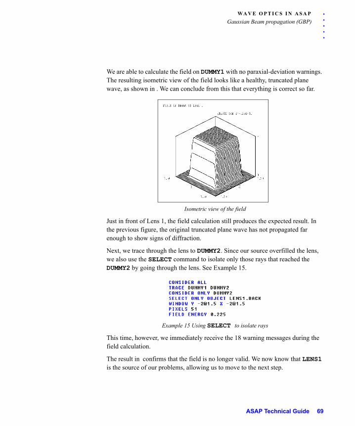
. . .
. .WA V E O P T I C S I N A S A P
Gaussian Beam propagation (GBP)
We are able to calculate the field on DUMMY1 with no paraxial-deviation warnings. The resulting isometric view of the field looks like a healthy, truncated plane wave, as shown in . We can conclude from this that everything is correct so far.
Isometric view of the field
Just in front of Lens 1, the field calculation still produces the expected result. In the previous figure, the original truncated plane wave has not propagated far enough to show signs of diffraction.
Next, we trace through the lens to DUMMY2. Since our source overfilled the lens, we also use the SELECT command to isolate only those rays that reached the DUMMY2 by going through the lens. See Example 15.
Example 15 Using SELECT to isolate rays
This time, however, we immediately receive the 18 warning messages during the field calculation.
The result in confirms that the field is no longer valid. We now know that LENS1 is the source of our problems, allowing us to move to the next step.
ASAP Technical Guide 69
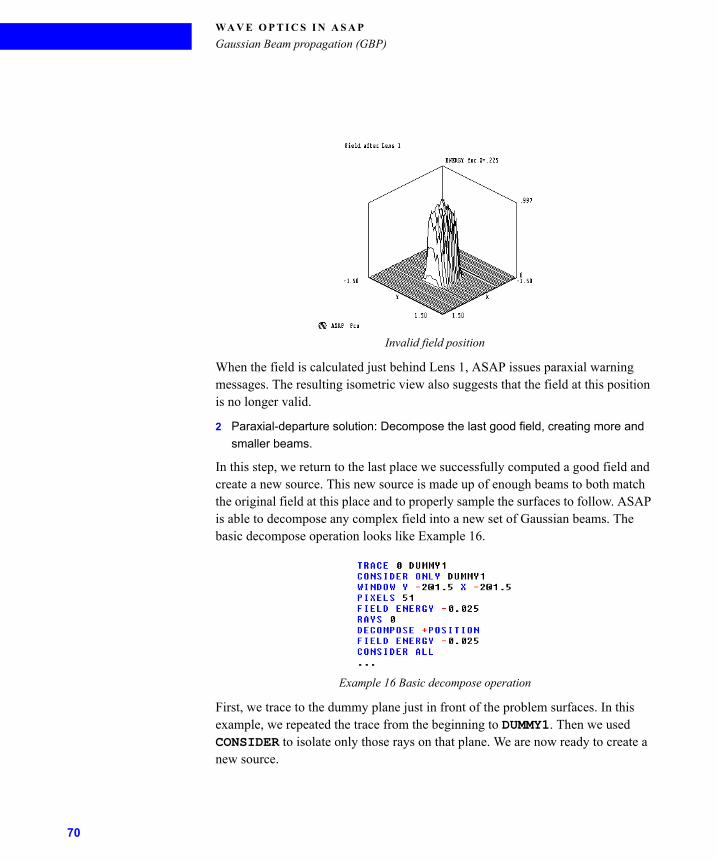
WA V E O P T I C S I N A S A P
Gaussian Beam propagation (GBP)
Invalid field position
When the field is calculated just behind Lens 1, ASAP issues paraxial warning messages. The resulting isometric view also suggests that the field at this position is no longer valid.
2 Paraxial-departure solution: Decompose the last good field, creating more and
smaller beams.
In this step, we return to the last place we successfully computed a good field and create a new source. This new source is made up of enough beams to both match the original field at this place and to properly sample the surfaces to follow. ASAP is able to decompose any complex field into a new set of Gaussian beams. The basic decompose operation looks like Example 16.
Example 16 Basic decompose operation
First, we trace to the dummy plane just in front of the problem surfaces. In this example, we repeated the trace from the beginning to DUMMY1. Then we used CONSIDER to isolate only those rays on that plane. We are now ready to create a new source.
70
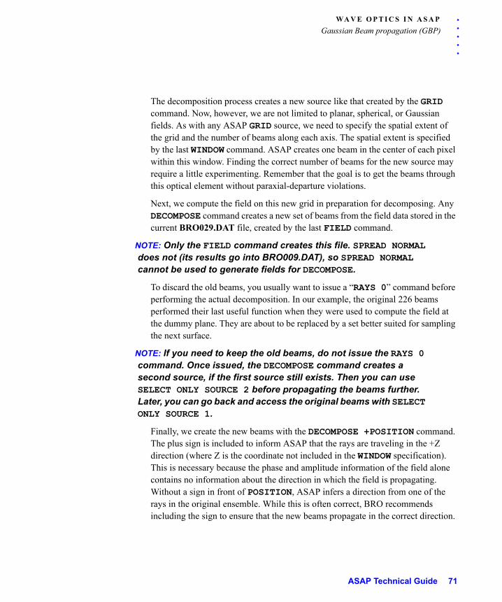
. . .
. .WA V E O P T I C S I N A S A P
Gaussian Beam propagation (GBP)
The decomposition process creates a new source like that created by the GRID command. Now, however, we are not limited to planar, spherical, or Gaussian fields. As with any ASAP GRID source, we need to specify the spatial extent of the grid and the number of beams along each axis. The spatial extent is specified by the last WINDOW command. ASAP creates one beam in the center of each pixel within this window. Finding the correct number of beams for the new source may require a little experimenting. Remember that the goal is to get the beams through this optical element without paraxial-departure violations.
Next, we compute the field on this new grid in preparation for decomposing. Any DECOMPOSE command creates a new set of beams from the field data stored in the current BRO029.DAT file, created by the last FIELD command.
NOTE: Only the FIELD command creates this file. SPREAD NORMAL does not (its results go into BRO009.DAT), so SPREAD NORMAL cannot be used to generate fields for DECOMPOSE.
To discard the old beams, you usually want to issue a “RAYS 0” command before performing the actual decomposition. In our example, the original 226 beams performed their last useful function when they were used to compute the field at the dummy plane. They are about to be replaced by a set better suited for sampling the next surface.
NOTE: If you need to keep the old beams, do not issue the RAYS 0 command. Once issued, the DECOMPOSE command creates a second source, if the first source still exists. Then you can use SELECT ONLY SOURCE 2 before propagating the beams further. Later, you can go back and access the original beams with SELECT ONLY SOURCE 1.
Finally, we create the new beams with the DECOMPOSE +POSITION command. The plus sign is included to inform ASAP that the rays are traveling in the +Z direction (where Z is the coordinate not included in the WINDOW specification). This is necessary because the phase and amplitude information of the field alone contains no information about the direction in which the field is propagating. Without a sign in front of POSITION, ASAP infers a direction from one of the rays in the original ensemble. While this is often correct, BRO recommends including the sign to ensure that the new beams propagate in the correct direction.
ASAP Technical Guide 71
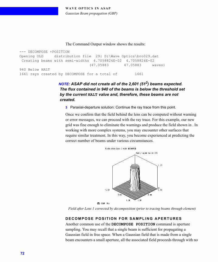
WA V E O P T I C S I N A S A P
Gaussian Beam propagation (GBP)
The Command Output window shows the results:
--- DECOMPOSE +POSITIONOpening OLD distribution file 29: D:\Wave Optics\bro029.dat Creating beams with semi-widths 4.7058824E-02 4.7058824E-02 (47.05883 47.05883 waves)940 Below HALT1661 rays created by DECOMPOSE for a total of 1661
NOTE: ASAP did not create all of the 2,601 (512) beams expected. The flux contained in 940 of the beams is below the threshold set by the current HALT value and, therefore, these beams are not created.
3 Paraxial-departure solution: Continue the ray trace from this point.
Once we confirm that the field behind the lens can be computed without warning or error messages, we can proceed with the ray trace. For this example, our new grid was fine enough to eliminate the warnings and produce the field shown in . In working with more complex systems, you may encounter other surfaces that require similar treatment. In this way, you become experienced at predicting the correct number of beams under various circumstances.
Field after Lens 1 corrected by decomposition (prior to tracing beams through element)
D E C O M P O S E P O S I T I O N F O R S A M P L I N G A P E R T U R E S
Another common use of the DECOMPOSE POSITION command is aperture sampling. You may recall that a single beam is sufficient for propagating a Gaussian field in free space. When a Gaussian field that is made from a single beam encounters a small aperture, all the associated field proceeds through with no
72
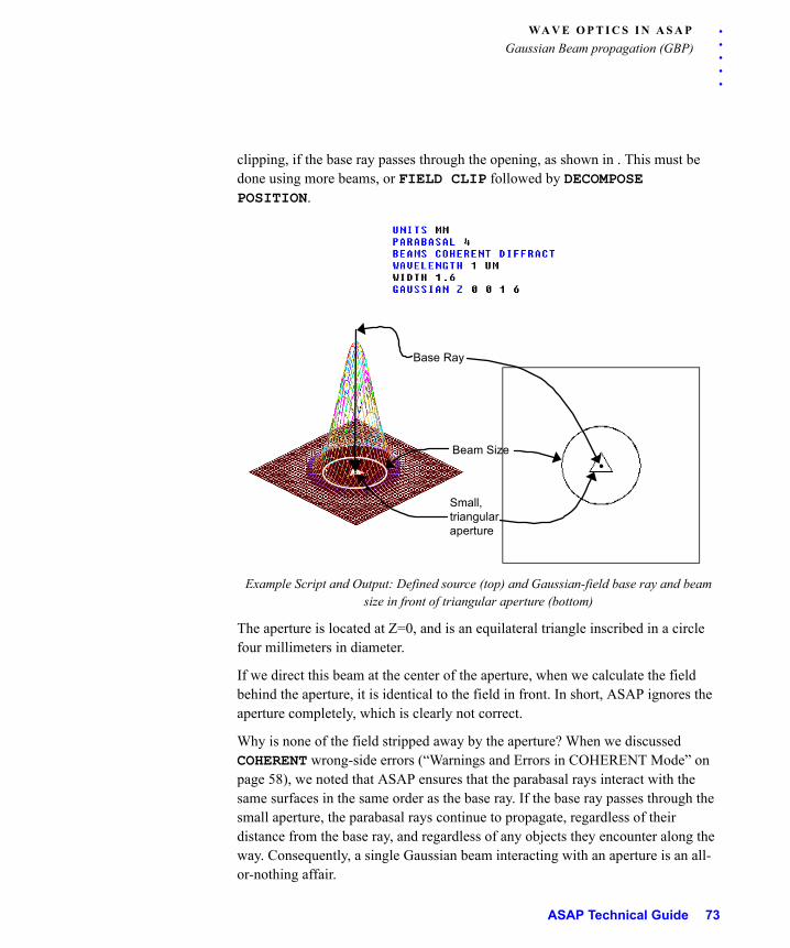
. . .
. .WA V E O P T I C S I N A S A P
Gaussian Beam propagation (GBP)
clipping, if the base ray passes through the opening, as shown in . This must be done using more beams, or FIELD CLIP followed by DECOMPOSE POSITION.
Example Script and Output: Defined source (top) and Gaussian-field base ray and beam size in front of triangular aperture (bottom)
The aperture is located at Z=0, and is an equilateral triangle inscribed in a circle four millimeters in diameter.
If we direct this beam at the center of the aperture, when we calculate the field behind the aperture, it is identical to the field in front. In short, ASAP ignores the aperture completely, which is clearly not correct.
Why is none of the field stripped away by the aperture? When we discussed COHERENT wrong-side errors (“Warnings and Errors in COHERENT Mode” on page 58), we noted that ASAP ensures that the parabasal rays interact with the same surfaces in the same order as the base ray. If the base ray passes through the small aperture, the parabasal rays continue to propagate, regardless of their distance from the base ray, and regardless of any objects they encounter along the way. Consequently, a single Gaussian beam interacting with an aperture is an all-or-nothing affair.
.Beam Size
.Small,triangularaperture
Base Ray
.
ASAP Technical Guide 73
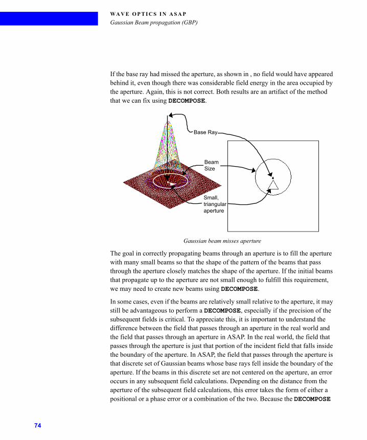
WA V E O P T I C S I N A S A P
Gaussian Beam propagation (GBP)
If the base ray had missed the aperture, as shown in , no field would have appeared behind it, even though there was considerable field energy in the area occupied by the aperture. Again, this is not correct. Both results are an artifact of the method that we can fix using DECOMPOSE.
Gaussian beam misses aperture
The goal in correctly propagating beams through an aperture is to fill the aperture with many small beams so that the shape of the pattern of the beams that pass through the aperture closely matches the shape of the aperture. If the initial beams that propagate up to the aperture are not small enough to fulfill this requirement, we may need to create new beams using DECOMPOSE.
In some cases, even if the beams are relatively small relative to the aperture, it may still be advantageous to perform a DECOMPOSE, especially if the precision of the subsequent fields is critical. To appreciate this, it is important to understand the difference between the field that passes through an aperture in the real world and the field that passes through an aperture in ASAP. In the real world, the field that passes through the aperture is just that portion of the incident field that falls inside the boundary of the aperture. In ASAP, the field that passes through the aperture is that discrete set of Gaussian beams whose base rays fell inside the boundary of the aperture. If the beams in this discrete set are not centered on the aperture, an error occurs in any subsequent field calculations. Depending on the distance from the aperture of the subsequent field calculations, this error takes the form of either a positional or a phase error or a combination of the two. Because the DECOMPOSE
..
Base Ray
BeamSize
Small,triangularaperture
74
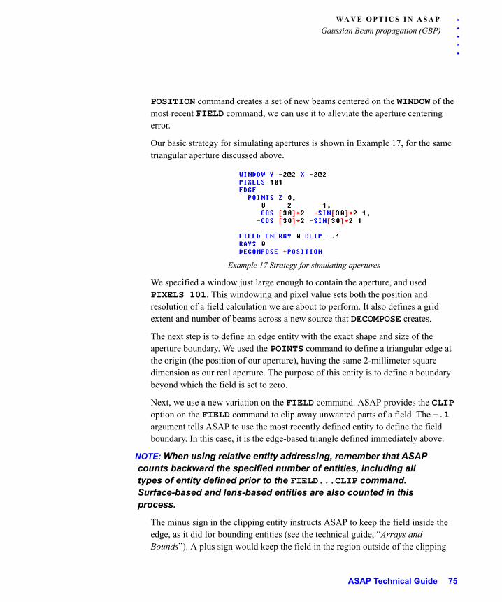
. . .
. .WA V E O P T I C S I N A S A P
Gaussian Beam propagation (GBP)
POSITION command creates a set of new beams centered on the WINDOW of the most recent FIELD command, we can use it to alleviate the aperture centering error.
Our basic strategy for simulating apertures is shown in Example 17, for the same triangular aperture discussed above.
Example 17 Strategy for simulating apertures
We specified a window just large enough to contain the aperture, and used PIXELS 101. This windowing and pixel value sets both the position and resolution of a field calculation we are about to perform. It also defines a grid extent and number of beams across a new source that DECOMPOSE creates.
The next step is to define an edge entity with the exact shape and size of the aperture boundary. We used the POINTS command to define a triangular edge at the origin (the position of our aperture), having the same 2-millimeter square dimension as our real aperture. The purpose of this entity is to define a boundary beyond which the field is set to zero.
Next, we use a new variation on the FIELD command. ASAP provides the CLIP option on the FIELD command to clip away unwanted parts of a field. The -.1 argument tells ASAP to use the most recently defined entity to define the field boundary. In this case, it is the edge-based triangle defined immediately above.
NOTE: When using relative entity addressing, remember that ASAP counts backward the specified number of entities, including all types of entity defined prior to the FIELD...CLIP command. Surface-based and lens-based entities are also counted in this process.
The minus sign in the clipping entity instructs ASAP to keep the field inside the edge, as it did for bounding entities (see the technical guide, “Arrays and Bounds”). A plus sign would keep the field in the region outside of the clipping
ASAP Technical Guide 75
WA V E O P T I C S I N A S A P
Gaussian Beam propagation (GBP)
edge. Always use an explicit “+” to specify this part of the field, when clipping with an entity.
We calculated the field at Z=0 by using the depth coordinate in the FIELD command. This is the plane in which the new beams are created, as well. It does not need to be the current location of the beams, if they have been stopped on a dummy plane in front of the aperture. This is the location of the physical aperture, however, which is the appropriate place to calculate the field and create the new beams.
CAUTION: We emphasize the difference between aperture sampling and the sampling of optical elements, as discussed previously. If the object being sampled is an optical surface, rather than an aperture, the field is calculated a small distance in front of the surface, so that no beams are created exactly on a surface. This is what we did in the previous example of lens sampling. Failure to do so causes ray-trace problems for ASAP, just as it does with geometric rays. With aperture sampling, however, this is not an issue, and the beams can be created in the plane of the opening.
Defining a special edge entity is not the only way to define a clipping boundary. In fact, the WINDOW itself is an ideal means of simulating a rectangular aperture. An edge entity, however, allows us to specify more complex clipping boundaries. Objects that are derived from either edge-based or surface-based entities can also be used for this purpose. Edge entities, however, are simpler and more convenient
76
. . .
. .WA V E O P T I C S I N A S A P
Gaussian Beam propagation (GBP)
in most cases. For more information, see the sidebar, “Using Objects as Clipping Boundaries”.
U S I N G O B J E C T S A S C L I P P I N G B O U N D A R I E S
We have used an edge entity to define a clipping boundary in our example. Several advantages exist in clipping with edge entities rather than objects, and therefore we recommend clipping with edges. It is, however, possible to clip with one of your objects. If the CLIP argument is followed by an unsigned number (either absolute/integer or relative/fraction without an explicit plus or minus sign), the argument refers to an object that will be used for the clipping. CAUTION: clipping by objects retains the portion of the field that intersects the clipped object. This
leads to a result that is intuitive for mirrors and lenses, keeping that portion of the field that intersects the object, while discarding what spills over the sides. On the other hand, opaque planes with apertures that were cut out do not behave as we would expect. ASAP retains that part of the field that falls on the opaque part of the aperture (the logical “true” part of the object), and discards the part of the field that fills the hole (the logical “false” part of the object). Other issues associated with object clipping usually make edges the better choice.
ASAP Technical Guide 77
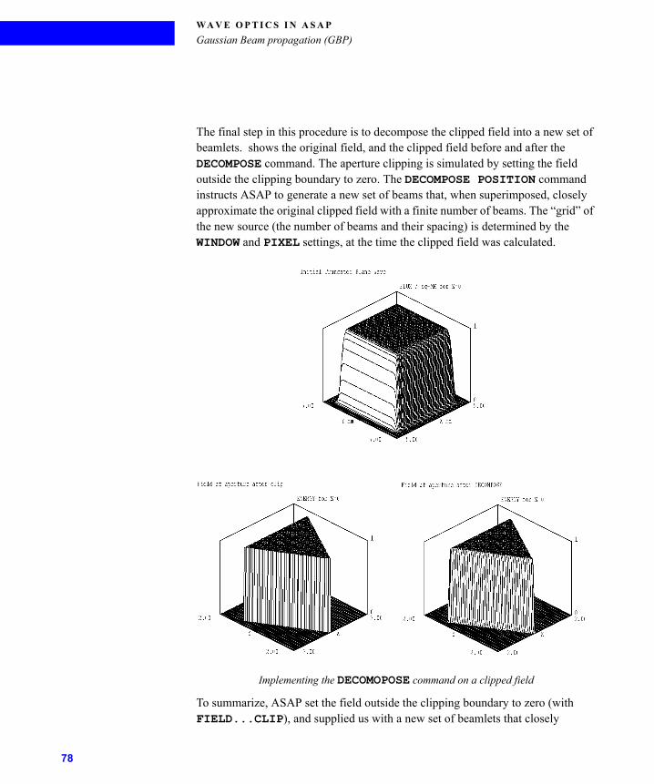
WA V E O P T I C S I N A S A P
Gaussian Beam propagation (GBP)
The final step in this procedure is to decompose the clipped field into a new set of beamlets. shows the original field, and the clipped field before and after the DECOMPOSE command. The aperture clipping is simulated by setting the field outside the clipping boundary to zero. The DECOMPOSE POSITION command instructs ASAP to generate a new set of beams that, when superimposed, closely approximate the original clipped field with a finite number of beams. The “grid” of the new source (the number of beams and their spacing) is determined by the WINDOW and PIXEL settings, at the time the clipped field was calculated.
Implementing the DECOMOPOSE command on a clipped field
To summarize, ASAP set the field outside the clipping boundary to zero (with FIELD...CLIP), and supplied us with a new set of beamlets that closely
78
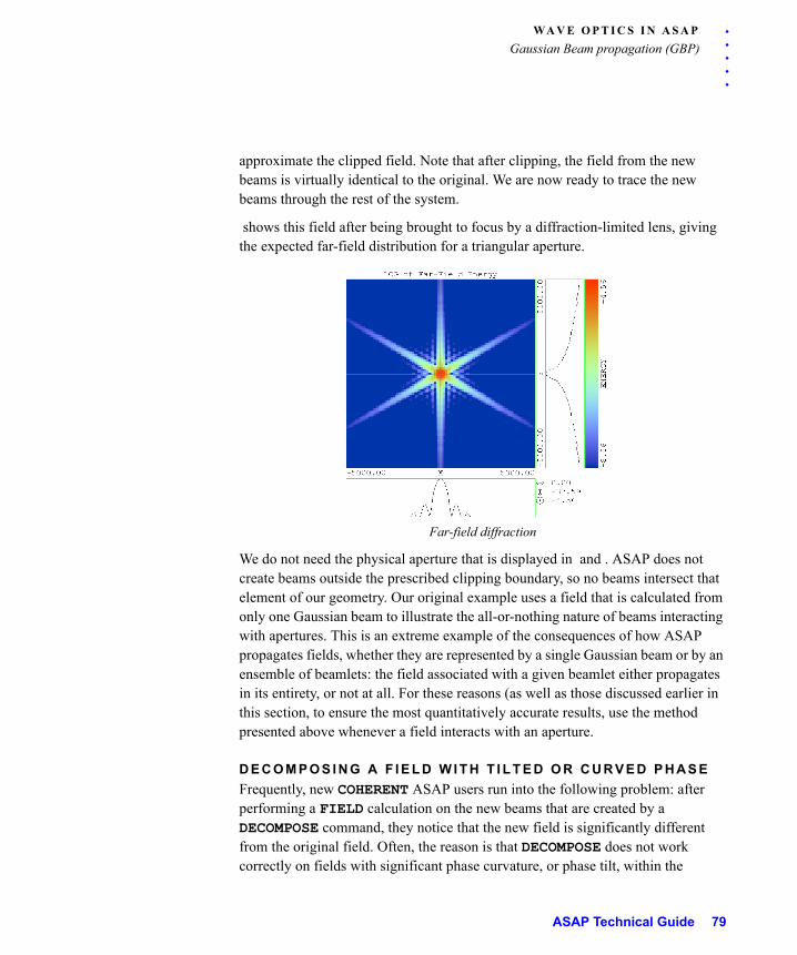
. . .
. .WA V E O P T I C S I N A S A P
Gaussian Beam propagation (GBP)
approximate the clipped field. Note that after clipping, the field from the new beams is virtually identical to the original. We are now ready to trace the new beams through the rest of the system.
shows this field after being brought to focus by a diffraction-limited lens, giving the expected far-field distribution for a triangular aperture.
Far-field diffraction
We do not need the physical aperture that is displayed in and . ASAP does not create beams outside the prescribed clipping boundary, so no beams intersect that element of our geometry. Our original example uses a field that is calculated from only one Gaussian beam to illustrate the all-or-nothing nature of beams interacting with apertures. This is an extreme example of the consequences of how ASAP propagates fields, whether they are represented by a single Gaussian beam or by an ensemble of beamlets: the field associated with a given beamlet either propagates in its entirety, or not at all. For these reasons (as well as those discussed earlier in this section, to ensure the most quantitatively accurate results, use the method presented above whenever a field interacts with an aperture.
D E C O M P O S I N G A F I E L D W I T H T I L T E D O R C U R V E D P H A S E
Frequently, new COHERENT ASAP users run into the following problem: after performing a FIELD calculation on the new beams that are created by a DECOMPOSE command, they notice that the new field is significantly different from the original field. Often, the reason is that DECOMPOSE does not work correctly on fields with significant phase curvature, or phase tilt, within the
ASAP Technical Guide 79
WA V E O P T I C S I N A S A P
Gaussian Beam propagation (GBP)
calculation window. All fields must be calculated in one of the global planes, which is not always the ideal reference frame in which to apply DECOMPOSE.
ASAP can still perform DECOMPOSE on fields with tilted or curved phases. For small tilts and curvature, ASAP generally does well on its own. When the departure from a plane becomes large, the DECOMPOSE POSITION command has three special options that allow for a more robust result when using DECOMPOSE. We accomplish this by using the CON, DIV, and PLA options.
The CON and DIV options refer to converging and diverging spherical wave fronts, respectively. With DECOMPOSE POSITION x y z CON, we inform ASAP that the new source should converge to a center-of-curvature point at x y z. No sign is required on POSITION, since a direction is implied by the use of the CON option.
NOTE: An estimate of the radius of curvature is generally good enough for these purposes. ASAP needs a little help in reducing the overall curvature while the DECOMPOSE is being performed. See the sidebar, “Estimating the radius of curvature of a wave front” on page 81.
Similarly, by issuing DECOMPOSE POSITION x y z DIV, ASAP knows that the field has a phase curvature that diverges from the center-of-curvature point x y z. In both cases, ASAP subtracts a reference sphere with the same curvature to create a flat (or nearly flat) phase. ASAP performs the DECOMPOSE, and adds the original phase curvature back to the new beam set. An example of DECOMPOSE POSITION, with the DIV option, appears in “Correctly modeling Fresnel coefficients”, which begins on page -100.
In a similar way, DECOMPOSE POSITION a b c PLA allows us to describe a plane of equal phase, with the direction cosines of the normal to that plane given by a b c. ASAP subtracts out a reference plane with the same tilt to create an untilted phase, performs the DECOMPOSE, and adds the original phase tilt back to the new beam set. In this situation, you can use the STATS DIR command to obtain the direction cosines of the desired plane.
If the phase has both curvature and tilt, the DECOMPOSE is done with the CON or DIV options, as explained above, but the x y z center of curvature is an off-axis point.
In “Decomposing Fields” on page 65, we mentioned three other less frequently used applications. The modeling of arbitrary fields can be accomplished with
80
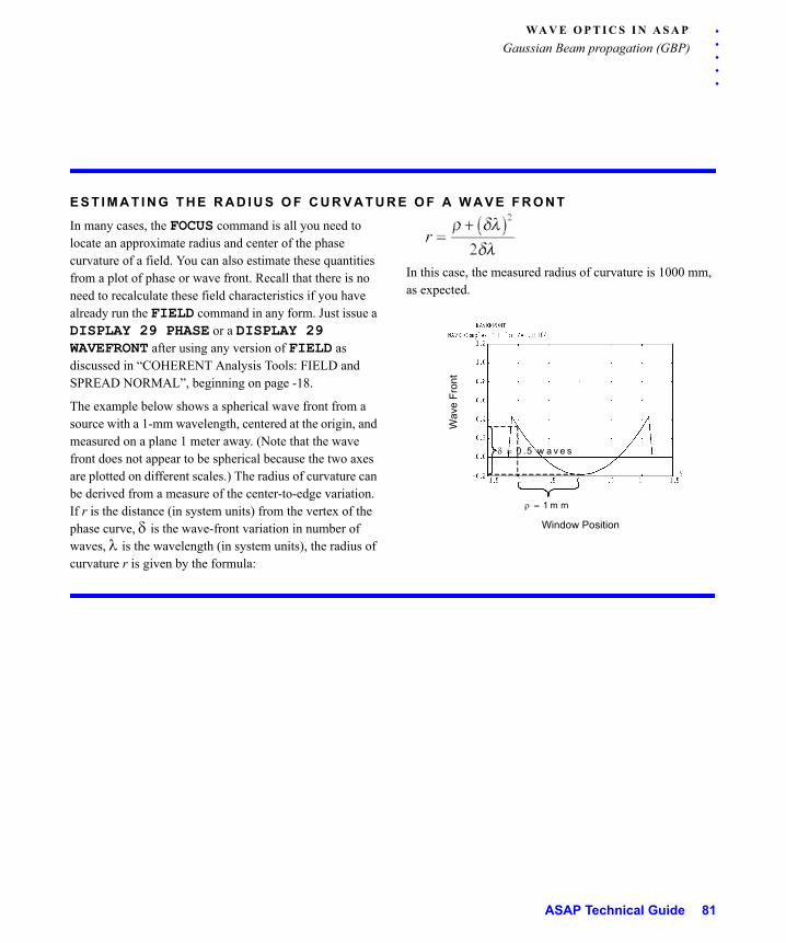
. . .
. .WA V E O P T I C S I N A S A P
Gaussian Beam propagation (GBP)
E S T I M A T I N G T H E R A D I U S O F C U R V A T U R E O F A W A V E F R O N T
In many cases, the FOCUS command is all you need to locate an approximate radius and center of the phase curvature of a field. You can also estimate these quantities from a plot of phase or wave front. Recall that there is no need to recalculate these field characteristics if you have already run the FIELD command in any form. Just issue a DISPLAY 29 PHASE or a DISPLAY 29 WAVEFRONT after using any version of FIELD as discussed in “COHERENT Analysis Tools: FIELD and SPREAD NORMAL”, beginning on page -18.
The example below shows a spherical wave front from a source with a 1-mm wavelength, centered at the origin, and measured on a plane 1 meter away. (Note that the wave front does not appear to be spherical because the two axes are plotted on different scales.) The radius of curvature can be derived from a measure of the center-to-edge variation. If r is the distance (in system units) from the vertex of the phase curve, is the wave-front variation in number of waves, is the wavelength (in system units), the radius of curvature r is given by the formula:
In this case, the measured radius of curvature is 1000 mm, as expected.
Window Position
Wa
ve F
ront
0 .5 w a v e s
1 m m
ASAP Technical Guide 81
WA V E O P T I C S I N A S A P
Gaussian Beam propagation (GBP)
either DECOMPOSE POSITION or DIRECTION depending on the field size. This application type is described below. Two other types of applications (namely, creating highly divergent sources and obtaining correct FRESNEL transmission and reflection coefficients) can be accomplished only with DECOMPOSE DIRECTION. These two are described later.
U S I N G D E C O M P O S E T O M O D E L A N A R B I T R A R Y F I E L D
So far, we have discussed methods for modeling only truncated plane waves, spherical waves, and Gaussians beams. What can be done for other fields? If, for example, you have amplitude and phase information in a plane, either from measurements or from evaluating a known function, there is a way to propagate this field using ASAP. Now that we have introduced the DECOMPOSE POSITION command, we have the tools to model any arbitrary field.
Recall that the first step in using DECOMPOSE POSITION is to calculate the complex (real and imaginary) field with the FIELD command. ASAP places it in the file, BRO029.DAT. The DECOMPOSE POSITION command generates a new set of Gaussian beams that simulates this field. If we could generate our own BRO029.DAT file and decompose it, this would allow us to generate a set of beamlets simulating any field. See .
82
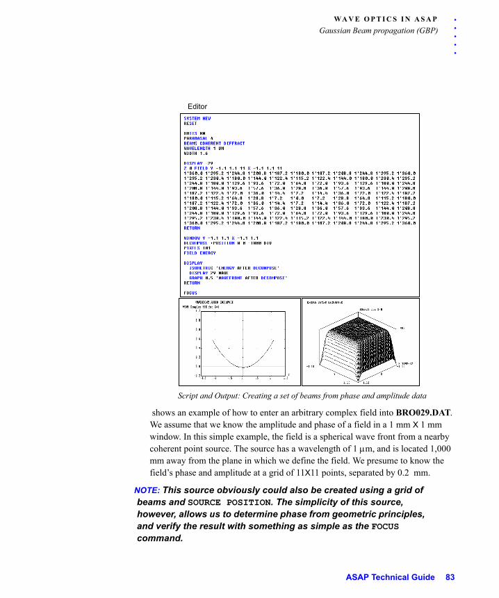
. . .
. .WA V E O P T I C S I N A S A P
Gaussian Beam propagation (GBP)
Script and Output: Creating a set of beams from phase and amplitude data
shows an example of how to enter an arbitrary complex field into BRO029.DAT. We assume that we know the amplitude and phase of a field in a 1 mm X 1 mm window. In this simple example, the field is a spherical wave front from a nearby coherent point source. The source has a wavelength of 1 m, and is located 1,000 mm away from the plane in which we define the field. We presume to know the field’s phase and amplitude at a grid of 11X11 points, separated by 0.2 mm.
NOTE: This source obviously could also be created using a grid of beams and SOURCE POSITION. The simplicity of this source, however, allows us to determine phase from geometric principles, and verify the result with something as simple as the FOCUS command.
Editor
ASAP Technical Guide 83
WA V E O P T I C S I N A S A P
Gaussian Beam propagation (GBP)
The first steps shown in Example 18 are the usual commands used to define the critical parameters for a new ASAP COHERENT source:
Example 18 Defining the critical parameters for COHERENT
The following line sets up ASAP to receive a header line and the numerical data describing the field:
DISPLAY -29
The DISPLAY command is familiar. We have seen commands like DISPLAY 29 PHASE or DISPLAY 29 WAVEFRONT before, but this time there is a minus sign in front of 29, and no keyword following. This sign tells ASAP that we will define our own field, rather than ASAP reading an existing distribution file into memory (the usual task of the DISPLAY command). Subsequent lines are used to define that field.
NOTE: The format of BRO029.DAT is binary, so we do not have the option of creating this file using a text editor. Instead, we will use ASAP commands to build this data file.
The next line is a header describing the format of the data to follow:
Z 0 FIELD Y -1.1 1.1 11 X -1.1 1.1 11
Recall that when ASAP creates BRO029.DAT for us, it does so with the FIELD command based on the current window and pixel settings. All that information is contained in this line. The data output is in the same format as that produced by the Example 19.
Example 19 FIELD command
The parameter 11, which appears twice in the header, is the size of the complex data array to be entered. ASAP expects an 11X11 block of complex numbers. That much is easy. Getting the window correct may be more difficult. In this example, we have a data point every 0.2 mm on a 1mm X 1mm grid. ASAP pixel boundaries go right up to the edge of the window, but the values we need correspond to the
84
. . .
. .WA V E O P T I C S I N A S A P
Gaussian Beam propagation (GBP)
pixel centers. The window must be slightly oversized to cause ASAP to assign the appropriate x and y coordinates to values. (See the sidebar, “Window and Pixel details” on page 86.)
The next eleven lines contain the field data—eleven complex numbers on each line. There are several possible formats for these data values. ASAP ultimately stores the values as two separate arrays—one for the real and one for the imaginary component at each point. Most laboratory measurements, however, express the complex numbers as amplitude and phase. ASAP is able to accept the number pairs in either form, depending on the character used to separate the two components:
• Amplitude and Phase in degrees: 2'3 represents the complex number with amplitude 2 and phase 3 degrees, or (converting to radians and exponential format: 2.0e0.052i).
• Real and Imaginary: 1.997‘0.1047 is the same complex number expressed in terms of the real and imaginary components (real = Acos () and imaginary = Asin (), where A is amplitude and is phase).
One complication arises in many cases—an ASAP command line is normally limited to 128 characters. In our example, we have only eleven points, and little precision in the numbers. As a result, we are easily able to stay within the 128-character limit. In many practical situations, more samples and more precision may be available. Consequently, it may be necessary to place more than 128 characters on each line. Two solutions are:
1 Use the comma (,) character to allow long, continuous lists to occupy more than
one record (line) in your command script.
2 Use $FAST to read in lines of virtually unlimited length.
ASAP Technical Guide 85
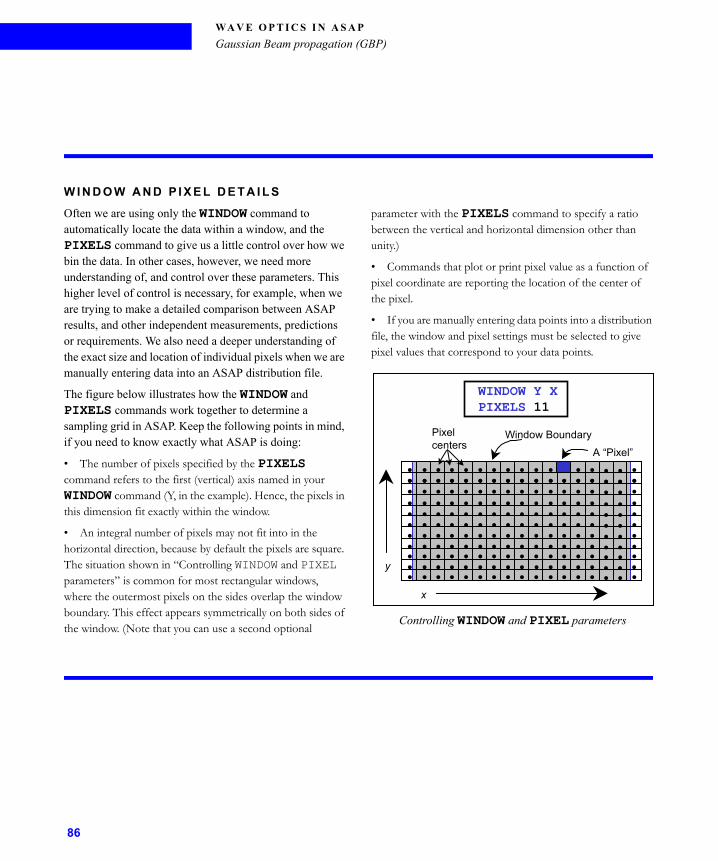
WA V E O P T I C S I N A S A P
Gaussian Beam propagation (GBP)
W I N D O W A N D P I X E L D E T A I L S
Often we are using only the WINDOW command to automatically locate the data within a window, and the PIXELS command to give us a little control over how we bin the data. In other cases, however, we need more understanding of, and control over these parameters. This higher level of control is necessary, for example, when we are trying to make a detailed comparison between ASAP results, and other independent measurements, predictions or requirements. We also need a deeper understanding of the exact size and location of individual pixels when we are manually entering data into an ASAP distribution file.
The figure below illustrates how the WINDOW and PIXELS commands work together to determine a sampling grid in ASAP. Keep the following points in mind, if you need to know exactly what ASAP is doing:
• The number of pixels specified by the PIXELS command refers to the first (vertical) axis named in your WINDOW command (Y, in the example). Hence, the pixels in this dimension fit exactly within the window.
• An integral number of pixels may not fit into in the horizontal direction, because by default the pixels are square. The situation shown in “Controlling WINDOW and PIXEL parameters” is common for most rectangular windows, where the outermost pixels on the sides overlap the window boundary. This effect appears symmetrically on both sides of the window. (Note that you can use a second optional
parameter with the PIXELS command to specify a ratio between the vertical and horizontal dimension other than unity.)
• Commands that plot or print pixel value as a function of pixel coordinate are reporting the location of the center of the pixel.
• If you are manually entering data points into a distribution file, the window and pixel settings must be selected to give pixel values that correspond to your data points.
Controlling WINDOW and PIXEL parameters
.. . . . . . . . . . . . . . .. .. . . . . . . . . . . . . . .. .. . . . . . . . . . . . . . .. .. . . . . . . . . . . . . . .. .. . . . . . . . . . . . . . .. .. . . . . . . . . . . . . . .. .. . . . . . . . . . . . . . ..
.. . . . . . . . . . . . . . ..
.. . . . . . . . . . . . . . .. .. . . . . . . . . . . . . . ..
.. . . . . . . . . . . . . . .. .. . . . . . . . . . . . . . ..y
x
Window BoundaryPixelcenters
A “Pixel”
WINDOW Y XPIXELS 11
86
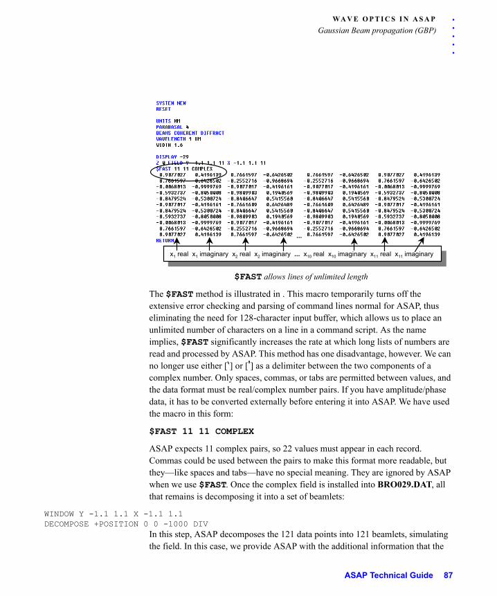
. . .
. .WA V E O P T I C S I N A S A P
Gaussian Beam propagation (GBP)
$FAST allows lines of unlimited length
The $FAST method is illustrated in . This macro temporarily turns off the extensive error checking and parsing of command lines normal for ASAP, thus eliminating the need for 128-character input buffer, which allows us to place an unlimited number of characters on a line in a command script. As the name implies, $FAST significantly increases the rate at which long lists of numbers are read and processed by ASAP. This method has one disadvantage, however. We can no longer use either [‘] or ['] as a delimiter between the two components of a complex number. Only spaces, commas, or tabs are permitted between values, and the data format must be real/complex number pairs. If you have amplitude/phase data, it has to be converted externally before entering it into ASAP. We have used the macro in this form:
$FAST 11 11 COMPLEX
ASAP expects 11 complex pairs, so 22 values must appear in each record. Commas could be used between the pairs to make this format more readable, but they—like spaces and tabs—have no special meaning. They are ignored by ASAP when we use $FAST. Once the complex field is installed into BRO029.DAT, all that remains is decomposing it into a set of beamlets:
WINDOW Y -1.1 1.1 X -1.1 1.1DECOMPOSE +POSITION 0 0 -1000 DIV
In this step, ASAP decomposes the 121 data points into 121 beamlets, simulating the field. In this case, we provide ASAP with the additional information that the
...
x1 real x1 imaginary x2 real x2 imaginary ... x10 real x10 imaginary x11 real x11 imaginaryx1 real x1 imaginary x2 real x2 imaginary ... x10 real x10 imaginary x11 real x11 imaginary
ASAP Technical Guide 87
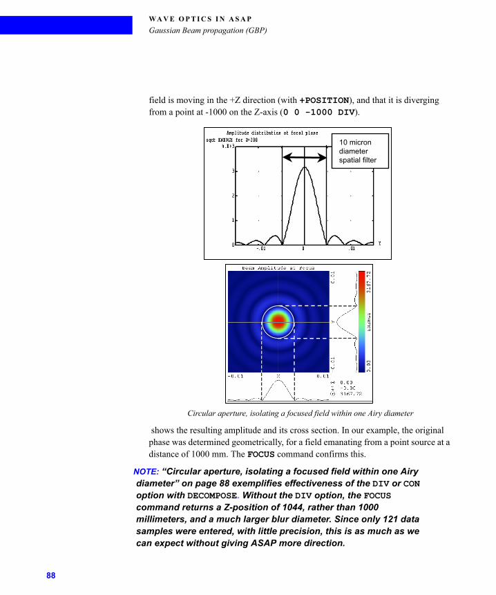
WA V E O P T I C S I N A S A P
Gaussian Beam propagation (GBP)
field is moving in the +Z direction (with +POSITION), and that it is diverging from a point at -1000 on the Z-axis (0 0 -1000 DIV).
Circular aperture, isolating a focused field within one Airy diameter
shows the resulting amplitude and its cross section. In our example, the original phase was determined geometrically, for a field emanating from a point source at a distance of 1000 mm. The FOCUS command confirms this.
NOTE: “Circular aperture, isolating a focused field within one Airy diameter” on page 88 exemplifies effectiveness of the DIV or CON option with DECOMPOSE. Without the DIV option, the FOCUS command returns a Z-position of 1044, rather than 1000 millimeters, and a much larger blur diameter. Since only 121 data samples were entered, with little precision, this is as much as we can expect without giving ASAP more direction.
10 microndiameterspatial filter
88
. . .
. .WA V E O P T I C S I N A S A P
Gaussian Beam propagation (GBP)
D E C O M P O S E D I R E C T I O N F O R V E R Y S M A L L F I E L D S
Now consider a situation where a very small aperture is introduced at the focus of a diffraction-limited lens. The aperture might be functioning as a spatial filter in a coherent beam. In this case, the diameter of the spatial filter may be close to the size of the radiation wavelength. Furthermore, within that small diameter the focused field may have a non-uniform flux distribution. If we try to deal with this situation using DECOMPOSE POSITION, we are likely to create individual beamlets so small that they violate the paraxial condition from the moment of their origin. A coherent plane wave with wavelength 632.8 nanometers is focussed by an f /6.25 lens system onto an aperture plate. We want to model a 10-micron circular aperture that is used to isolate the field contained within the Airy diameter. To do this with DECOMPOSE POSITION, with 41x41 beams, for example, would cause the creation of individual beamlets that are smaller than a wavelength. ASAP issues this warning message:
Warning *** Beam height in waves = .308347 1620 *** Beam height in waves = .308347
As we noted previously in “Warnings and Error Messages”, which began on page -58, these beamlets are not a solution to a paraxial wave equation. Although it might appear that we have reached the limit of the Gaussian beam summation method, the DECOMPOSE DIRECTION command offers a solution in situations like this.
The DECOMPOSE DIRECTION command performs a Fourier transform on the field in angle space, to create new set of beamlets. This method is similar, in principle, to the methods of Fourier optics, where a field of arbitrary complexity can be decomposed into a set of plane waves of varying propagation directions. When DECOMPOSE DIRECTION is used, all the new beams have the same size and their base rays are at the same location (the center of the original field distribution), but each has a different direction. The flux weighting of each beamlet is dependent on the spatial frequency content within that component in the original field. The individual beamlets may represent fields that are much larger than the original field, but since each beamlet has a different direction or linear phase tilt, they destructively interfere to give zero field, where appropriate. Another FIELD command that is issued on this new set of beams for the same WINDOW and PIXELS, with care, returns a flux distribution almost identical to the original, except where significant evanescent components are present (see the sidebar, “Evanescent Waves” on page 90).
ASAP Technical Guide 89
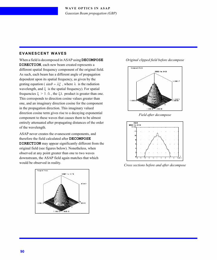
WA V E O P T I C S I N A S A P
Gaussian Beam propagation (GBP)
E V A N E S C E N T W A V E S
When a field is decomposed in ASAP using DECOMPOSE DIRECTION, each new beam created represents a different spatial frequency component of the original field. As such, each beam has a different angle of propagation dependent upon its spatial frequency, as given by the grating equation ( , where is the radiation wavelength, and is the spatial frequency). For spatial frequencies > , the product is greater than one. This corresponds to direction cosine values greater than one, and an imaginary direction cosine for the component in the propagation direction. This imaginary valued direction cosine term gives rise to a decaying exponential component to these waves that causes them to be almost entirely attenuated after propagating distances of the order of the wavelength.
ASAP never creates the evanescent components, and therefore the field calculated after DECOMPOSE DIRECTION may appear significantly different from the original field (see figures below). Nonetheless, when observed at any point greater than one to two waves downstream, the ASAP field again matches that which would be observed in reality.
Original clipped field before decompose
Field after decompose
Cross sections before and after decompose
sin
1
90
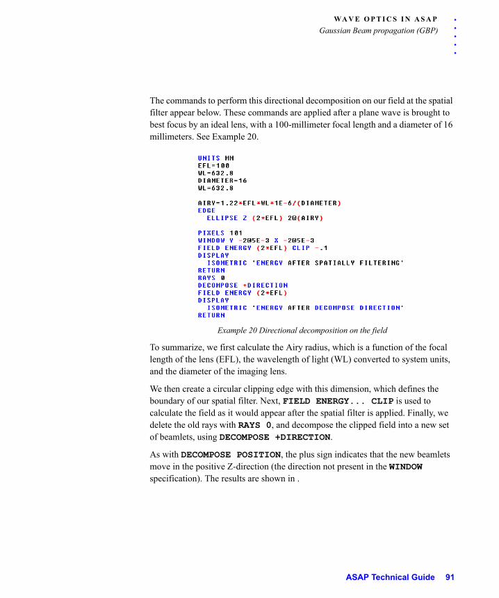
. . .
. .WA V E O P T I C S I N A S A P
Gaussian Beam propagation (GBP)
The commands to perform this directional decomposition on our field at the spatial filter appear below. These commands are applied after a plane wave is brought to best focus by an ideal lens, with a 100-millimeter focal length and a diameter of 16 millimeters. See Example 20.
Example 20 Directional decomposition on the field
To summarize, we first calculate the Airy radius, which is a function of the focal length of the lens (EFL), the wavelength of light (WL) converted to system units, and the diameter of the imaging lens.
We then create a circular clipping edge with this dimension, which defines the boundary of our spatial filter. Next, FIELD ENERGY... CLIP is used to calculate the field as it would appear after the spatial filter is applied. Finally, we delete the old rays with RAYS 0, and decompose the clipped field into a new set of beamlets, using DECOMPOSE +DIRECTION.
As with DECOMPOSE POSITION, the plus sign indicates that the new beamlets move in the positive Z-direction (the direction not present in the WINDOW specification). The results are shown in .
ASAP Technical Guide 91
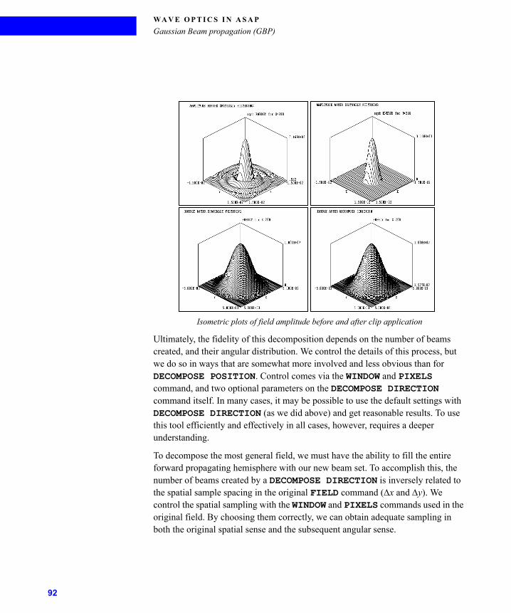
WA V E O P T I C S I N A S A P
Gaussian Beam propagation (GBP)
Isometric plots of field amplitude before and after clip application
Ultimately, the fidelity of this decomposition depends on the number of beams created, and their angular distribution. We control the details of this process, but we do so in ways that are somewhat more involved and less obvious than for DECOMPOSE POSITION. Control comes via the WINDOW and PIXELS command, and two optional parameters on the DECOMPOSE DIRECTION command itself. In many cases, it may be possible to use the default settings with DECOMPOSE DIRECTION (as we did above) and get reasonable results. To use this tool efficiently and effectively in all cases, however, requires a deeper understanding.
To decompose the most general field, we must have the ability to fill the entire forward propagating hemisphere with our new beam set. To accomplish this, the number of beams created by a DECOMPOSE DIRECTION is inversely related to the spatial sample spacing in the original FIELD command (x and y). We control the spatial sampling with the WINDOW and PIXELS commands used in the original field. By choosing them correctly, we can obtain adequate sampling in both the original spatial sense and the subsequent angular sense.
92
. . .
. .WA V E O P T I C S I N A S A P
Gaussian Beam propagation (GBP)
The number of beams required to fill the entire forward propagating hemisphere is approximately the
(EQ 13)
Equation 14
where N is the dimension of the FFT array used inside ASAP (the FFT size is set by the FTSIZE command), is the radiation wavelength, and x and y are the sample spacing in the field:
(EQ 15)
Equation 16
(EQ 17)
Equation 18
The number of beams calculated in this way gives the amount required to fill the forward propagating hemisphere at this sampling. Some beams may not be created due to a calculated flux weight that falls below the HALT or CUTOFF settings, or due to their evanescent nature (see sidebar, “Evanescent Waves” on page 90). Also, ASAP never creates more than the total number of pixels in the FFT array (determined by the FTSIZE command), regardless of , x, and y values. If x and y are so large that the angular sampling increment is tiny, DECOMPOSE DIRECTION reaches the FTSIZE limitation before filling the hemisphere, and stops creating beams. In this case, the x and y chosen are probably too large to appropriately sample the field, and should be changed. Another source of these extremely small increments in angle space could be that the field was actually not so large as to preclude using DECOMPOSE POSITION in the first place.
If we issue the DECOMPOSE DIRECTION command without any arguments, as we did in , ASAP creates enough beams to fill the hemisphere, up to a default maximum (10% of the FFT array size as set by the FTSIZE command). We can change this behavior by using the first (m) optional parameter on the DECOMPOSE
ASAP Technical Guide 93
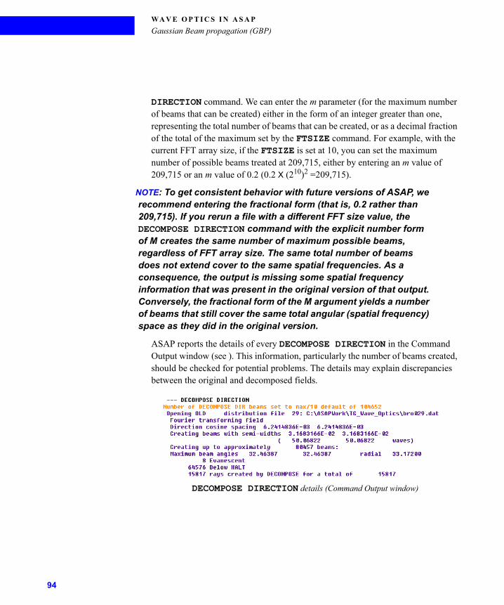
WA V E O P T I C S I N A S A P
Gaussian Beam propagation (GBP)
DIRECTION command. We can enter the m parameter (for the maximum number of beams that can be created) either in the form of an integer greater than one, representing the total number of beams that can be created, or as a decimal fraction of the total of the maximum set by the FTSIZE command. For example, with the current FFT array size, if the FTSIZE is set at 10, you can set the maximum number of possible beams treated at 209,715, either by entering an m value of 209,715 or an m value of 0.2 (0.2 X (210)2 =209,715).
NOTE: To get consistent behavior with future versions of ASAP, we recommend entering the fractional form (that is, 0.2 rather than 209,715). If you rerun a file with a different FFT size value, the DECOMPOSE DIRECTION command with the explicit number form of M creates the same number of maximum possible beams, regardless of FFT array size. The same total number of beams does not extend cover to the same spatial frequencies. As a consequence, the output is missing some spatial frequency information that was present in the original version of that output. Conversely, the fractional form of the M argument yields a number of beams that still cover the same total angular (spatial frequency) space as they did in the original version.
ASAP reports the details of every DECOMPOSE DIRECTION in the Command Output window (see ). This information, particularly the number of beams created, should be checked for potential problems. The details may explain discrepancies between the original and decomposed fields.
DECOMPOSE DIRECTION details (Command Output window)
94
. . .
. .WA V E O P T I C S I N A S A P
Gaussian Beam propagation (GBP)
CAUTION: Whenever the number of beams created is exactly the number specified or implied by m, you should be concerned. ASAP almost certainly terminated beam creation before it was able to fill the entire forward hemisphere. This error has eliminated the highest spatial frequencies present in the original field, which in turn may be critical to the fidelity of the field we want to simulate. Ultimately, a FIELD command should be used to carefully compare the energy distribution before and after the decomposition, as a final check on the process.
The second argument of the DECOMPOSE DIRECTION command is a, the maximum half-angle in degrees, out to which new beams are created. This parameter is used to purposely limit the range of angles in the decomposed beam set. Their angular sampling frequency is still a function of N, , x, and y, as shown in the equation above, but truncation of the beams occurs beyond a. The a parameter is useful if the beams created are subsequently passed through a limiting aperture, such as a lens, mirror, or slit. In this case, no good reason may exist to spend the extra time in creating and tracing beamlets that will be terminated by the aperture and never contribute to the final result. Any attempt to graphically verify the fidelity of such a source may be misleading, however.
ASAP Technical Guide 95
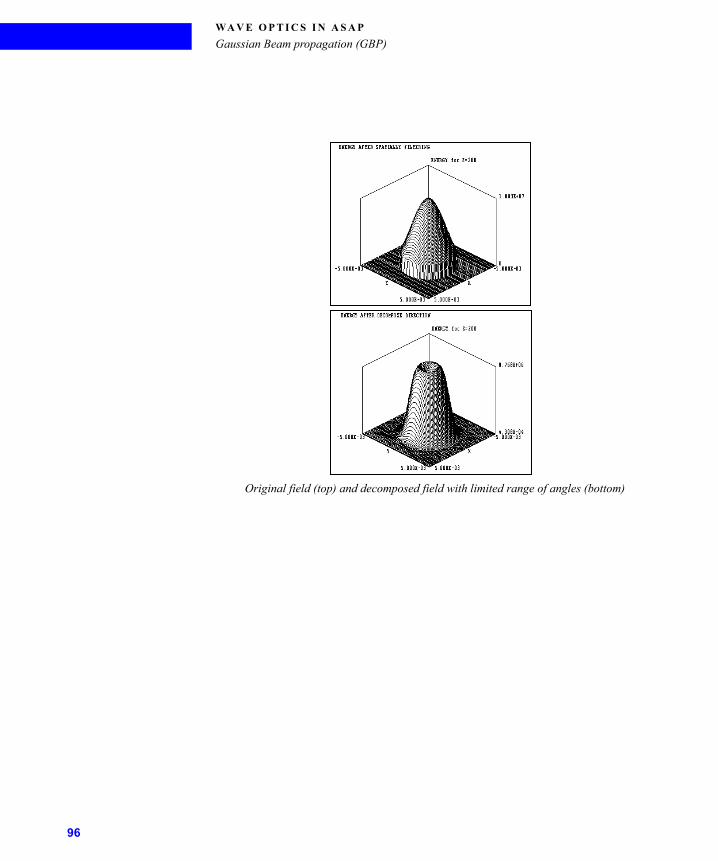
WA V E O P T I C S I N A S A P
Gaussian Beam propagation (GBP)
Original field (top) and decomposed field with limited range of angles (bottom)
96

. . .
. .WA V E O P T I C S I N A S A P
Gaussian Beam propagation (GBP)
shows a variation of our original example, where a smaller (6-micron) spatial filter was substituted into the system, and the a parameter was used to limit the field to 15 degrees, corresponding to a downstream aperture. Now the sharp cutoff of the central core of the Airy function requires beams at high angles to simulate the sharp edges in such a field. But if we limit the angle with the a parameter, the field after decomposing bears little resemblance to the original. Although this is not as reassuring as the previous result, the field is still valid if it is soon truncated by a circular aperture, subtending only a 15-degree half angle.
Even when we attempt to fill the entire forward hemisphere in the case currently under consideration, we still will not recover the exact field. This example is the same as shown in the sidebar, “Evanescent Waves” on page 90. Eight evanescent beams were never created, and their absence is sufficient to significantly change the appearance of the field beyond the aperture.
C R E A T I N G A S M A L L , H I G H L Y D I V E R G E N T S O U R C E W I T H
D E C O M P O S E D I R E C T O N
The DECOMPOSE DIRECTION command can be used to create accurate representations of highly divergent sources such as laser diodes. If you create a small, highly divergent source, where the width of the source is approximately of the order of the wavelength or smaller, the individual Gaussian beamlets will violate the paraxial condition, since the Gaussian beam is only a solution to a paraxial wave equation. Because a Gaussian field with a width smaller than one wavelength is not a mode of a general, non-paraxial wave equation, it will not maintain its Gaussian shape as it propagates.
When ASAP propagates the Gaussian beamlets downstream from the plane of the source creation, it does so by the ray tracing techniques described previously. In doing so, the individual Gaussian beamlets remain Gaussian. This induces errors in fields calculated downstream from a very small source, unless the DECOMPOSE DIRECTION command is applied to the original source prior to propagation. The DECOMPOSE DIRECTION command performs a Fourier transform on the original field to create a new set of beamlets—each traveling at a different angle and weighted, based on the spatial frequency content of the original source. Most importantly, each of the new beamlets is wider than those in the original field and will, therefore, propagate correctly in ASAP.
While the DECOMPOSE DIRECTION command used in this way always gives the correct result, it adds extra steps and time to the ASAP run. The improvement
ASAP Technical Guide 97

WA V E O P T I C S I N A S A P
Gaussian Beam propagation (GBP)
in accuracy of the DECOMPOSE DIRECTION method increases continuously as the original source width decreases.
An example that gives a feel for the source widths, for which this improvement becomes significant, is shown below in . The script shows an initial source consisting of single Gaussian beam with an ASAP half-width of 0.5 waves.
The two plots each show two separate curves of the resulting beam profiles after 100 mm of propagation. One of the beam profiles is due to an initial source represented by a single Gaussian beam, and the other profile is due to an initial source created by performing a DECOMPOSE DIRECTION on the initial field prior to propagation.
The plot on the left shows the case for the initial source with a half-width of 0.5-waves. In it, you can see that there is a large difference between the curve representing the source due to the single Gaussian beam without DECOMPOSE, and the source due to the correct field obtained using DECOMPOSE DIRECTION.
The plot on the right shows the case for the initial source with a half-width of 2 waves. In it, you can see that the difference between the curve representing the source due to the single Gaussian beam without DECOMPOSE, and the source due to the correct field obtained using DECOMPOSE DIRECTION is much smaller than it was in the 0.5-wave case.
Additionally, the correct field in the 0.5-wave case shows a loss due the attenuation of evanescent components of approximately two percent. For the wider, 2-wave source case, the losses due to evanescent waves are negligible.
98
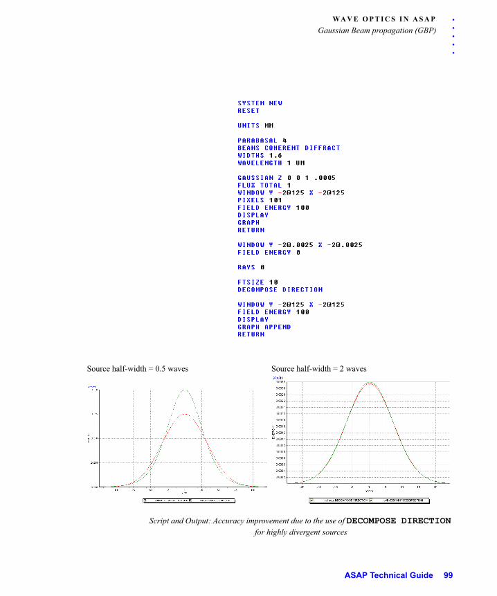
. . .
. .WA V E O P T I C S I N A S A P
Gaussian Beam propagation (GBP)
Script and Output: Accuracy improvement due to the use of DECOMPOSE DIRECTION for highly divergent sources
Source half-width = 0.5 waves Source half-width = 2 waves
ASAP Technical Guide 99
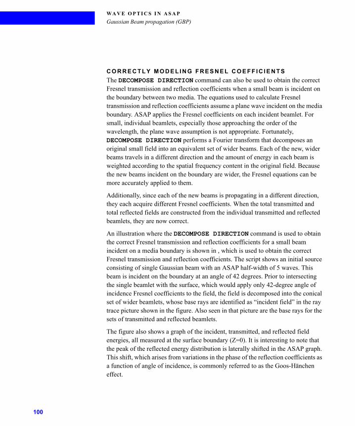
WA V E O P T I C S I N A S A P
Gaussian Beam propagation (GBP)
C O R R E C T L Y M O D E L I N G F R E S N E L C O E F F I C I E N T S
The DECOMPOSE DIRECTION command can also be used to obtain the correct Fresnel transmission and reflection coefficients when a small beam is incident on the boundary between two media. The equations used to calculate Fresnel transmission and reflection coefficients assume a plane wave incident on the media boundary. ASAP applies the Fresnel coefficients on each incident beamlet. For small, individual beamlets, especially those approaching the order of the wavelength, the plane wave assumption is not appropriate. Fortunately, DECOMPOSE DIRECTION performs a Fourier transform that decomposes an original small field into an equivalent set of wider beams. Each of the new, wider beams travels in a different direction and the amount of energy in each beam is weighted according to the spatial frequency content in the original field. Because the new beams incident on the boundary are wider, the Fresnel equations can be more accurately applied to them.
Additionally, since each of the new beams is propagating in a different direction, they each acquire different Fresnel coefficients. When the total transmitted and total reflected fields are constructed from the individual transmitted and reflected beamlets, they are now correct.
An illustration where the DECOMPOSE DIRECTION command is used to obtain the correct Fresnel transmission and reflection coefficients for a small beam incident on a media boundary is shown in , which is used to obtain the correct Fresnel transmission and reflection coefficients. The script shows an initial source consisting of single Gaussian beam with an ASAP half-width of 5 waves. This beam is incident on the boundary at an angle of 42 degrees. Prior to intersecting the single beamlet with the surface, which would apply only 42-degree angle of incidence Fresnel coefficients to the field, the field is decomposed into the conical set of wider beamlets, whose base rays are identified as “incident field” in the ray trace picture shown in the figure. Also seen in that picture are the base rays for the sets of transmitted and reflected beamlets.
The figure also shows a graph of the incident, transmitted, and reflected field energies, all measured at the surface boundary (Z=0). It is interesting to note that the peak of the reflected energy distribution is laterally shifted in the ASAP graph. This shift, which arises from variations in the phase of the reflection coefficients as a function of angle of incidence, is commonly referred to as the Goos-Hänchen effect.
100
. . .
. .WA V E O P T I C S I N A S A P
Gaussian Beam propagation (GBP)
DECOMPOSE DIRECTION command is used to obtain the correct Fresnel transmission and reflection coefficients
D E C O M P O S I N G P O L A R I Z E D F I E L D S
The DECOMPOSE command creates a set of beams that correspond to the field within the current BRO029.dat file. It is one of the four commands, along with GRID, RAYSET, and GAUSSIAN, that allows for the creation of COHERENT sources. As such, if polarization analysis is being performed, a POLARIZ command must be issued prior to the DECOMPOSE command. Also, if the field to be decomposed has significant amounts of orthogonal polarization components, a POLARIZ and DECOMPOSE pair must be issued for each component.
ASAP Technical Guide 101
WA V E O P T I C S I N A S A P
Gaussian Beam propagation (GBP)
An example is shown below.
POLARIZ XDECOMPOSE POSITIONPOLARIZ YDECOMPOSE POSITIONPOLARIZ ZDECOMPOSE POSITION
NOTE: Because of the method employed in ASAP, the results are sometimes more accurate when you skip one of the polarization components if the amount of energy in that component is several orders of magnitude less than the other components. In other words, if the field is polarized primarily in X and Y with only a tiny Z component, it may be more accurate to just decompose the X and Y components and skip the Z decomposition. To determine whether the component with the small amount of energy should be decomposed or not, we must examine how well the total fields match before and after DECOMPOSE.
References—Gaussian Beam• Arnaud, J. “Nonorthogonal Optical Waveguides and Resonators,” Bell System
Technical Journal (November 1970): 2311-2348.
• Arnaud, J. “Representation of Gaussian beams by complex rays,” Applied Optics 24, no. 4, (February 15, 1985): 33-50.
• Greynolds, A. “Propagation of generally astigmatic Gaussian beams along skew ray paths,” Proceedings of SPIE: Diffractive Phenomena in Optical Engineering Applications 560 (1985): 33-50.
• Greynolds, A. “Vector formulation of ray-equivalent method for general Gaussian beam propagation,” Proceedings of SPIE: Current Developments in Optical Engineering and Diffractive Phenomena 679 (1986): 129-133.
• Herlowski, R. et al. “Gaussian beam ray-equivalent modeling and optical design,” Applied Optics 22, no. 8, (April 15 1983): 1168-1174. (Erratum, Applied Optics 22, no. 20, (October 15, 1983): 3151.)
• Einziger, P. et al. “Gabor representation and aperture theory,” Journal of the Optical Society of America (JOSA) A 3, no. 4, (April 1986): 508-522.
• Felson, L. “Real spectra, complex spectra, compact spectra,” Journal of the Optical Society of America (JOSA) A 3, no. 4, (April 1986): 486-496.
102
. . .
. .Beam Propagation Method (BPM)
. . . . . . . . . . . . . . . . . . . . . . . . . . . . . . . . . . . . . . . . . . . . . . . . . . . . B E A M P R O P A G A T I O N M E T H O D ( B P M )
The term, BPM (beam propagation method) is used extensively in the optics literature. Although all the so-called BPM techniques propagate optical fields, there is a great variability in both the techniques used and how well they solve different types of optics problems. The ASAP BPM calculates the optical field in a series of evenly spaced planes in three-dimensional space. It uses a finite difference technique to solve the scalar or semi-vectorial Helmholtz equation. The field in each successive plane is calculated from discrete points in the previous plane. The optionally included higher-order derivatives can increase accuracy. This requires more calculation points from the previous field and, therefore, slows the calculation. While BPM is not as accurate as certain techniques such as Finite Difference Time Domain (FDTD) or Finite Element Time Domain (FETD), which perform full solutions to Maxwell’s equations, it is much faster.
BPM is used in ASAP to propagate fields through microstructures with dimensions of the order of the wavelength. Since BPM has more limitations and less capability than Gaussian beam ASAP, the former is typically used only for situations where the dimensions of the optical components are too small for Gaussian beam ASAP. BPM has three main limitations that are not present in Gaussian beam ASAP.
1 BPM calculates only the forward propagating component of the field. As such, it
will calculate the correct phase and relative energy distribution of the optical
field, but not the absolute energy.
2 In the highest accuracy mode, the angular divergence of the field is limited to
about 40 degrees.
3 BPM is semi-vectorial. This means that the optical axis of any birefringent media
must be oriented along one of the global X, Y, or Z axes.
BPM can model coupling in and out of fibers of all types (step-index, GRIN, multimode, dual-clad, shaped-tip, etc.) as well as propagation through micro optics and waveguides. Typical applications for BPM include telecom components, integrated optics, micro optics, photonic bandgap materials, and many more.
Second form of F IELD commandLearning to use BPM is quite easy. BPM is not separate software—it resides within ASAP inside of the FIELD (or FIELDBPM) command. Although the starting field for BPM must be created prior to BPM, the entire BPM including the specification of the starting field, the actual propagation of the field, and the
ASAP Technical Guide 103
Beam Propagation Method (BPM)
calculation of the intermediate and final fields are all performed with the FIELD (or FIELDBPM) command. This allows for simple, seamless transitions from macro-optics into micro-optics and back inside of the same ASAP INR file.
Steps for BPMASAP analysis, both INCOHERENT (geometrical) and COHERENT (Gaussian beam), is composed of four major steps:
1 System construction
2 Source creation
3 Ray tracing
4 Analysis
However, BPM does not fit well in this four-step model. BPM does not use any of the ASAP source commands. Instead, the starting field that gets propagated must exist as an array of complex numbers in the same format as a BRO029.DAT file. Each complex number corresponds to the field value of a single pixel. Also, there are no rays and, therefore, there is no ray tracing. Instead, the field propagation, using the finite difference BPM, takes place when the FIELDBPM command is issued. Additionally, although geometry is created in the same fashion as with ASAP GBP, only the media boundaries and indices of the media are used in the BPM calculation. Surface treatments such as coatings and scatter properties are ignored. The only analysis command available in BPM is FIELDBPM.
The steps for BPM are as follows.
1 Construct the system geometries and media.
2 Issue the appropriate UNITS and WAVELENGTH commands.
3 Identify the file to be used for the starting field.
4 Choose a FIELD parameter to store in the BRO009.DAT file.
5 Choose the propagation distance and number of intermediate fields calculated.
6 Specify the boundary conditions to be used (or use default absorbing boundary
conditions).
7 Choose the accuracy setting (or use default ACCURACY LOW setting).
8 Issue the FIELDBPM command which propagates the field and performs the
analysis.
Each of these eight steps are expanded on in the following sections.
104
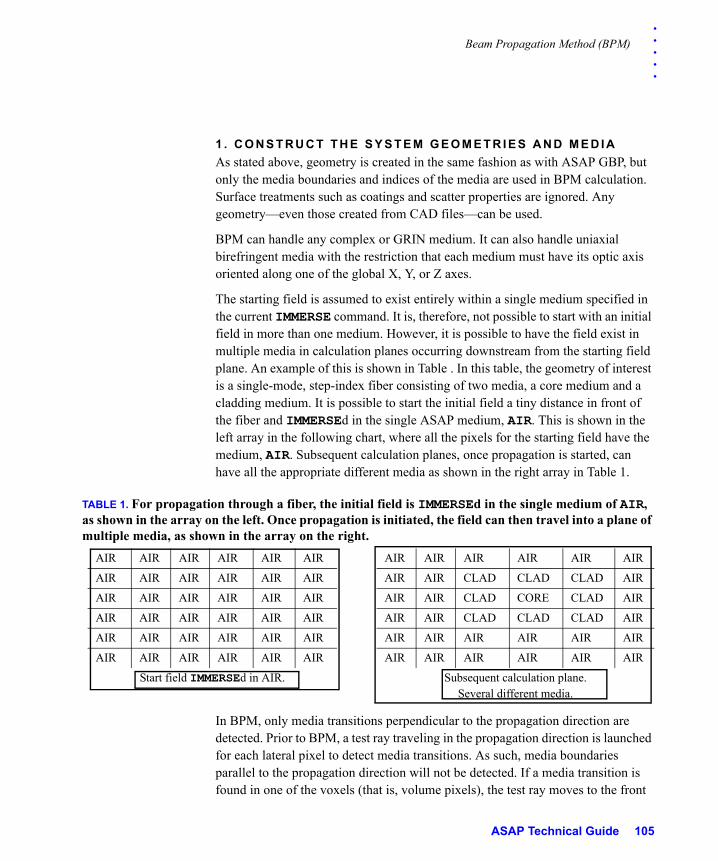
. . .
. .Beam Propagation Method (BPM)
1 . C O N S T R U C T T H E S Y S T E M G E O M E T R I E S A N D M E D I A
As stated above, geometry is created in the same fashion as with ASAP GBP, but only the media boundaries and indices of the media are used in BPM calculation. Surface treatments such as coatings and scatter properties are ignored. Any geometry—even those created from CAD files—can be used.
BPM can handle any complex or GRIN medium. It can also handle uniaxial birefringent media with the restriction that each medium must have its optic axis oriented along one of the global X, Y, or Z axes.
The starting field is assumed to exist entirely within a single medium specified in the current IMMERSE command. It is, therefore, not possible to start with an initial field in more than one medium. However, it is possible to have the field exist in multiple media in calculation planes occurring downstream from the starting field plane. An example of this is shown in Table . In this table, the geometry of interest is a single-mode, step-index fiber consisting of two media, a core medium and a cladding medium. It is possible to start the initial field a tiny distance in front of the fiber and IMMERSEd in the single ASAP medium, AIR. This is shown in the left array in the following chart, where all the pixels for the starting field have the medium, AIR. Subsequent calculation planes, once propagation is started, can have all the appropriate different media as shown in the right array in Table 1.
In BPM, only media transitions perpendicular to the propagation direction are detected. Prior to BPM, a test ray traveling in the propagation direction is launched for each lateral pixel to detect media transitions. As such, media boundaries parallel to the propagation direction will not be detected. If a media transition is found in one of the voxels (that is, volume pixels), the test ray moves to the front
TABLE 1. For propagation through a fiber, the initial field is IMMERSEd in the single medium of AIR, as shown in the array on the left. Once propagation is initiated, the field can then travel into a plane of multiple media, as shown in the array on the right.
AIR AIR AIR AIR AIR AIR AIR AIR AIR AIR AIR AIR
AIR AIR AIR AIR AIR AIR AIR AIR CLAD CLAD CLAD AIR
AIR AIR AIR AIR AIR AIR AIR AIR CLAD CORE CLAD AIR
AIR AIR AIR AIR AIR AIR AIR AIR CLAD CLAD CLAD AIR
AIR AIR AIR AIR AIR AIR AIR AIR AIR AIR AIR AIR
AIR AIR AIR AIR AIR AIR AIR AIR AIR AIR AIR AIR
Start field IMMERSEd in AIR. Subsequent calculation plane.Several different media.
ASAP Technical Guide 105
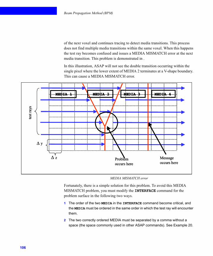
Beam Propagation Method (BPM)
of the next voxel and continues tracing to detect media transitions. This process does not find multiple media transitions within the same voxel. When this happens the test ray becomes confused and issues a MEDIA MISMATCH error at the next media transition. This problem is demonstrated in .
In this illustration, ASAP will not see the double transition occurring within the single pixel where the lower extent of MEDIA 2 terminates at a V-shape boundary. This can cause a MEDIA MISMATCH error.
MEDIA MISMATCH error
Fortunately, there is a simple solution for this problem. To avoid this MEDIA MISMATCH problem, you must modify the INTERFACE command for the problem surface in the following two ways.
1 The order of the two MEDIA in the INTERFACE command become critical, and
the MEDIA must be ordered in the same order in which the test ray will encounter
them.
2 The two correctly ordered MEDIA must be separated by a comma without a
space (the space commonly used in other ASAP commands). See Example 20.
y
z Problemoccurs here
Messageoccurs here
test
ray
s
MEDIA 1 MEDIA 2 MEDIA 3 MEDIA 4
y
z Problemoccurs here
Messageoccurs here
test
ray
s
MEDIA 1 MEDIA 2 MEDIA 3 MEDIA 4MEDIA 1MEDIA 1 MEDIA 2MEDIA 2 MEDIA 3MEDIA 3 MEDIA 4MEDIA 4
106
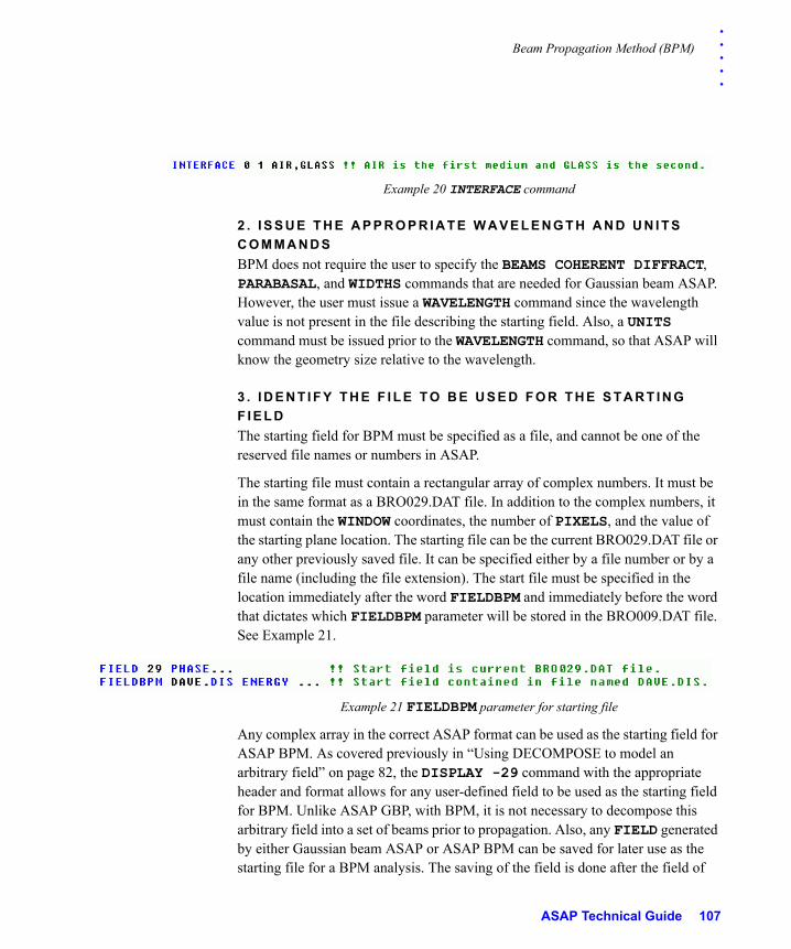
. . .
. .Beam Propagation Method (BPM)
Example 20 INTERFACE command
2 . I S S U E T H E A P P R O P R I A T E W A V E L E N G T H A N D U N I T S
C O M M A N D S
BPM does not require the user to specify the BEAMS COHERENT DIFFRACT, PARABASAL, and WIDTHS commands that are needed for Gaussian beam ASAP. However, the user must issue a WAVELENGTH command since the wavelength value is not present in the file describing the starting field. Also, a UNITS command must be issued prior to the WAVELENGTH command, so that ASAP will know the geometry size relative to the wavelength.
3 . I D E N T I F Y T H E F I L E T O B E U S E D F O R T H E S T A R T I N G
F I E L D
The starting field for BPM must be specified as a file, and cannot be one of the reserved file names or numbers in ASAP.
The starting file must contain a rectangular array of complex numbers. It must be in the same format as a BRO029.DAT file. In addition to the complex numbers, it must contain the WINDOW coordinates, the number of PIXELS, and the value of the starting plane location. The starting file can be the current BRO029.DAT file or any other previously saved file. It can be specified either by a file number or by a file name (including the file extension). The start file must be specified in the location immediately after the word FIELDBPM and immediately before the word that dictates which FIELDBPM parameter will be stored in the BRO009.DAT file. See Example 21.
Example 21 FIELDBPM parameter for starting file
Any complex array in the correct ASAP format can be used as the starting field for ASAP BPM. As covered previously in “Using DECOMPOSE to model an arbitrary field” on page 82, the DISPLAY -29 command with the appropriate header and format allows for any user-defined field to be used as the starting field for BPM. Unlike ASAP GBP, with BPM, it is not necessary to decompose this arbitrary field into a set of beams prior to propagation. Also, any FIELD generated by either Gaussian beam ASAP or ASAP BPM can be saved for later use as the starting file for a BPM analysis. The saving of the field is done after the field of
ASAP Technical Guide 107
Beam Propagation Method (BPM)
interest has been calculated and resides in BRO029.DAT, and prior to the calculation of another field that would overwrite the field of interest in BRO029.DAT. This is accomplished by issuing the $COPY macro command followed by 29 (for BRO029.DAT), and then followed by name to be assigned to the saved file. Names of saved files specified without an extension default to a DAT extension. The file name must include the extension when later specified as a starting field for BPM. See Example 22.
Example 22 Example Scripts for $COPY
NOTE: Confirm that the starting field has the appropriate WINDOW size and number of PIXELS.
Unlike ASAP GBP, the window size and number of pixels used in BPM calculation is not derived from the most recent WINDOW and PIXELS command. Instead, the window size and number of pixels used in BPM calculation are the same as they were in the file of the starting field. Not only is the lateral size of BPM calculation window the same as the WINDOW size of the starting field, but also the size of the calculation window stays constant during the entire propagation. Therefore, if the lateral width of the field increases during propagation, you must ensure that the WINDOW size of the starting field is large enough so that its size is adequate for the expanding field throughout the entire BPM propagation. Additionally, the size of this window must also allow for the additional pixels that are required if absorbing boundary conditions are used. The default boundary condition uses one-third of the pixels in each direction (one-sixth of the pixels nearest each edge) to model a physically absorbing boundary. More detail on boundary conditions is given in step “6. Specify the boundary conditions to be used (or use default absorbing boundary conditions)” on page 111.
4 . C H O O S E F I E L D P A R A M E T E R T O S T O R E I N T H E
B R O 0 0 9 . D A T F I L E
The word immediately following the start file name or number specifies the FIELD parameter (PHASE, WAVEFRONT, REAL, IMAGINARY, MODULUS, AMPLITUDE, or ENERGY) that will be stored in the BRO009.DAT file as a result of the BPM calculation. Issuing the DISPLAY command accesses the values for
108
. . .
. .Beam Propagation Method (BPM)
this FIELD parameter. As is the case in ASAP GBP, all the complex field values for the resultant FIELDBPM calculation are stored in the BRO029.DAT file. Any of the other FIELD parameters can be accessed by issuing the DISPLAY 29 command followed by the parameter of interest. In the case of polarization analysis, you must first issue a POLARIZ command to distinguish the polarization component of interest. The ability to use DISPLAY 29 to access all the various field parameters without having to recalculate the field is important. The FIELDBPM calculation can take a lot of time, and it is never necessary to recalculate the field just to display a different field parameter. See Example 23.
Example 23 Specifying the FIELD parameter
5 . C H O O S E T H E P R O P A G A T I O N D I S T A N C E
F O R M A T T Y P E 1
The propagation distance is specified after the field parameter chosen for the BRO009.DAT file. Two different format types exist that can be used to specify the propagation distance for BPM. The first format type can be specified either by a single number, which corresponds to the propagation distance (in system units), or by specifying two numbers which correspond to the propagation distance followed by the number of calculation planes. A example of this first format type with the propagation distance specified is shown in Example 24.
Example 24 Format type 1
Both of the examples given above tell ASAP to propagate the starting field a distance of five system units. The second of the examples tells ASAP to make field calculations in three different, equally spaced planes, with the last of the three planes a distance of five from the starting field.
ASAP Technical Guide 109
Beam Propagation Method (BPM)
When multiple calculation planes are specified, the field parameters in each plane can be examined separately by referring to the number of the plane of interest. There are two issues that need to be understood to DISPLAY the desired FIELD parameter in a given calculation plane.
The default calculation plane is the final plane at the full propagation distance. The various FIELD parameters for it can be accessed in the standard fashion. See Example 25.
Example 25 Accessing FIELD parameters
In the general case of requesting N different calculation planes, ASAP stores the fields for N+1 different planes (the N calculation planes plus the starting field). In this case, plane 1 refers to the starting field and the final calculation plane is plane N+1, not plane N. This is different from the numbering method used for calculating the field in multiple planes using the FIELDSUM command with ASAP GBP. Gaussian beam ASAP calculates the field of a set of beams and not an initial field file. Also, unlike ASAP GBP, there is no additional time penalty for calculating the field in multiple planes with BPM. This is due to the fact that BPM always calculates the field in a series of successive planes until the final propagation distance is reached. This approach is required because the field values in any given plane are derived from the field values in the previous plane. Therefore, requesting additional calculation planes in the BPM just requires ASAP to store already calculated intermediate-plane field values.
The first format type of propagation distance specification that is used with multiple calculation planes is shown in Example 26.
Example 26 Format Type 1 with multiple calculation planes
110
. . .
. .Beam Propagation Method (BPM)
F O R M A T T Y P E 2
The second format type that can be used to specify the BPM propagation distance requires you to issue three numbers immediately following the field parameter chosen for the BRO009.DAT file. These three numbers correspond to the coordinate of the starting plane, the coordinate of the end plane, and the number of calculation planes. This format type is closer in style to the format used in Gaussian beam ASAP. If the coordinate of the first entry is different than the value in the file for the starting field, ASAP places the given starting field at the first coordinate value listed in the FIELDBPM command and propagates by a total distance given by the difference of the first two entries. This action effectively moves the starting plane of the field stored in the starting file to a new value that is different from the coordinate value of its creation. As was the case for multiple calculation planes using format type 1, ASAP stores the fields for N+1 different planes (the N calculation planes plus the starting field). Also, as already explained for format type 1, for DISPLAY purposes, the final calculation plane is the default plane, or it can be explicitly called as plane N+1. The starting field is again plane 1. An example of the FIELDBPM command using the format type 2 propagation distance specifier is shown in Example 27.
Example 27 FIELDBPM command using Format Type 2
6 . S P E C I F Y T H E B O U N D A R Y C O N D I T I O N S T O B E U S E D ( O R
U S E D E F A U L T A B S O R B I N G B O U N D A R Y C O N D I T I O N S )
The result of the field calculation using BPM is a function of how the boundaries at the edges of the calculation region are described (that is, boundary conditions or BC). As the propagating field encounters the edges of the calculation region, ASAP needs to know how the field should respond at the boundary. At real optical boundaries that divide two media, a portion of the field intersecting the boundary is reflected. Once reflected, this field will interact with the rest of the forward propagating field. Most often, the BPM calculation boundary is just a lateral truncation of the calculation extent and is unrelated to the real physical situation being modeled. In these cases, you would prefer that when the field reaches the boundary of the calculation region, it would not reflect back. In ASAP, this is accomplished by applying absorbing boundary conditions. In addition to the absorbing boundary conditions, ASAP allows for periodic, zero field, and totally reflective boundary conditions.
ASAP Technical Guide 111
Beam Propagation Method (BPM)
Two types of absorbing boundary conditions exist: physical (the default when the BC specifier is not present) and numerical (when the BC specifier is present without any following numbers). In the physically absorbing case, the boundary pixels are given absorption values that increase as the pixels get closer to the edge of the calculation window. The absorption values are assigned so as to minimize boundary reflections. In the case of the numerically absorbing boundary conditions, the pixels themselves lengthen as they get closer to the edge of the calculation window. Even though the numerically absorbing boundary conditions were implemented first in ASAP, the physically absorbing boundary conditions usually work better. Therefore, if no boundary condition is specified, the default is a physically absorbing boundary condition. This applies a physically absorbing layer to the outer one-third of the pixels (one-sixth on each edge) in each window dimension.
To apply boundary conditions other than the default cases described above, you must explicitly issue the letters BC followed by either one, two, or four numbers in the FIELDBPM command, following the description of the propagation distance. The numerical values used to indicate the desired type of user-specified boundary condition are indicated in Table 2.
TABLE 2. The numerical values used to specify the type of boundary condition.
If only one number is given after the letters BC, that type of boundary condition is applied at all four calculation window boundaries. If two numbers are given after the BC, they are applied to the first edge of both window dimensions and the second edge of both window dimensions, respectively. To specify different boundary conditions in the two different window dimensions, you must specify four numbers after the BC. Those four numbers correspond to the first edge of the first window dimension, the first edge of the second window dimension, the second edge of the first window dimension, and the second edge of the second window dimension, respectively.
BC < -1 Band of pixels at window that is physically absorbing
BC -1 Periodic boundary condition
BC 0 Zero field
BC 1 Totally reflective field
BC > 1 Band of pixels at window that is numerically absorbing
112
. . .
. .Beam Propagation Method (BPM)
It is also possible to further reduce the amount of radiation reflected by increasing the size of the absorbing region. This allows for a more gradual absorption and, therefore, less reflection. The size of the absorbing band relative to the total calculation window can be increased to a value that is different from the default one-third. This is done by entering a negative floating point fractional value, rather than the less than 1 value for the physically absorbing case, or by entering a positive floating point fractional value, rather than the greater than 1 value for the numerically absorbing case.
The periodic boundary conditions are useful for modeling periodic structures. In this case, the BPM calculation behaves as though the calculation window was one of a number of repeated cells in a periodic structure. For the periodic boundary conditions to give a correct calculation, both the media and the starting field (amplitude and phase) must be periodic.
If the situation being modeled has symmetry, it may be possible to reduce the BPM calculation time by applying the reflecting boundary conditions. This is typically done to one side of one window dimension or one side of both window dimensions, depending on the type of symmetry present. In this case, the field at the reflecting boundary behaves as though the situation on the outside of the boundary is a mirror image of the situation inside the boundary. The zero field boundary condition forces the value of the field at the boundary to a zero value. See Example 28.
Example 28 Various ASAP boundary specifications
7 . C H O O S E T H E A C C U R A C Y S E T T I N G ( O R U S E D E F A U L T
S E T T I N G F O R A C C U R A C Y L O W )
The accuracy of BPM drops as the propagation angle of the field increases, or the index change between successive pixels increases. ASAP can improve the accuracy of BPM calculation by including higher-order derivatives. You instruct ASAP to do this with the ACCURACY command, which has three available settings: LOW, MEDIUM, and HIGH. To achieve the greater accuracy, you must pay a significant time penalty. Fortunately, ASAP gives an estimate of the remaining
ASAP Technical Guide 113
Beam Propagation Method (BPM)
calculation time while the calculation is in progress. An initial two-dimensional calculation can be used as a quick way to determine the best ACCURACY. This is described in “2D propagation” on page 116. Table 3 gives a guideline for when the higher accuracy settings may be required.
As stated in step “3. Identify the file to be used for the starting field” on page 107, the WINDOW size and the number of PIXELS in the file of the starting field determine the lateral sampling size. Typically, lateral sampling must be at least as small as one-quarter to one-third of the vacuum wavelength divided by the maximum index. The vacuum wavelength, the minimum, maximum, and references indices, and the lateral sampling size in waves at the reference index are displayed in . An example of such a command output listing is shown below.
Sample Command Output window at the start of the BPM calculation
As stated previously, ASAP automatically chooses the best longitudinal sampling size. This choice is based on the ACCURACY setting, the lateral sampling size, and size of the index steps. The number of longitudinal steps is also given at the start of the BPM in the Command Output window.
The best indicator of whether the sampling sizes and ACCURACY setting are appropriate to yield a correct result is given by two numbers in the Command Output window during the calculation, under the header “Relative Flux”. These values change continuously during BPM calculation. For non-absorbing cases, the values should stay close to unity through the entire calculation. An example of three cases of the same calculation with three different ACCURACY settings is
TABLE 3. Guideline for higher-order accuracy settings
ACCURACY setting
Operator order
Max angle from axis
Comments
LOW 1 10 Fresnel/paraxial/weakly-guided approximation
MEDIUM 2 20
HIGH 3 40 Wide-angle and/or large, refractive index variations
114
. . .
. .Beam Propagation Method (BPM)
shown below. Note that as the ACCURACY setting goes from LOW to MEDIUM to HIGH, the “relative flux” values get closer to unity at the expense of greater calculation times. See .
Sample output for low, medium, and high ACCURACY settings
8 . I S S U E T H E F I E L D B P M C O M M A N D , W H I C H P R O P A G A T E S
T H E F I E L D A N D P E R F O R M S T H E A N A L Y S I S .
All the BPM calculations are launched by issuing the FIELDBPM command. It is possible to issue the FIELD command without the explicit BPM portion, and assume that ASAP will perform the BPM because of the file name or number given after FIELD. However, it is better form, and less prone to confusion, when the BPM portion is used to distinguish it from the FIELDSUM command. ASAP uses the information discussed in the previous seven sections for the parameters of BPM calculation. All the FIELD options used with ASAP GBP and found in FIELDSUM (such as ADD, MULTIPLY, and COUPLE) are available in the BPM. The results from BPM calculation go to the BRO009.DAT and BRO029.DAT files and are available.
Lastly, a few special issues are addressed separately: “Field coupling”, “2D propagation”, and “Transitioning between BPM and ASAP GBP”.
Fie ld coupl ingCoupling of fields in the BPM is similar to the coupling of fields ASAP GBP. The only difference is that, instead of coupling the current beam set in the given plane into the contents of BRO029.DAT, ASAP propagates the specified file and then couples it into the contents of BRO029.DAT. See Example 29.
ASAP Technical Guide 115
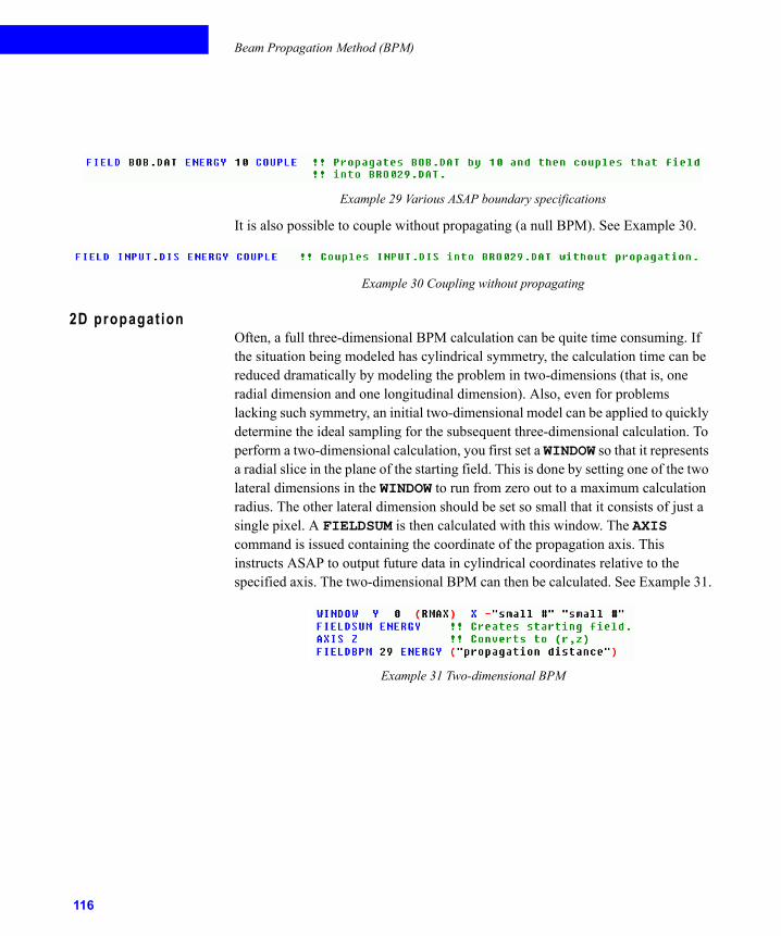
Beam Propagation Method (BPM)
Example 29 Various ASAP boundary specifications
It is also possible to couple without propagating (a null BPM). See Example 30.
Example 30 Coupling without propagating
2D propagat ionOften, a full three-dimensional BPM calculation can be quite time consuming. If the situation being modeled has cylindrical symmetry, the calculation time can be reduced dramatically by modeling the problem in two-dimensions (that is, one radial dimension and one longitudinal dimension). Also, even for problems lacking such symmetry, an initial two-dimensional model can be applied to quickly determine the ideal sampling for the subsequent three-dimensional calculation. To perform a two-dimensional calculation, you first set a WINDOW so that it represents a radial slice in the plane of the starting field. This is done by setting one of the two lateral dimensions in the WINDOW to run from zero out to a maximum calculation radius. The other lateral dimension should be set so small that it consists of just a single pixel. A FIELDSUM is then calculated with this window. The AXIS command is issued containing the coordinate of the propagation axis. This instructs ASAP to output future data in cylindrical coordinates relative to the specified axis. The two-dimensional BPM can then be calculated. See Example 31.
Example 31 Two-dimensional BPM
116
. . .
. .Beam Propagation Method (BPM)
Transi t ioning between BPM and ASAP GBPFor some systems, the appropriate ASAP model involves a combination of both BPM and GBP. Since BPM resides within the normal ASAP command structure, it is easy to transition between BPM and Gaussian beam ASAP. Going from Gaussian beam ASAP to BPM is as easy as saving the final Gaussian beam field and using that field as the starting field for BPM. Going from BPM to ASAP GBP requires one additional step. In this case, the final BPM field must be turned into Gaussian beams by use of the DECOMPOSE command. This command was covered in the section “Gaussian Beam propagation (GBP)” on page 8.
ExamplesSee “Appendix A: BPM Examples” on page 119 for example scripts of BPM.
ASAP Technical Guide 117

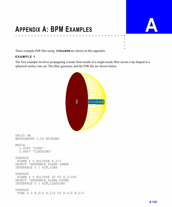
. . . . .
. . . . . . . . . . . . . . . . . . . . . . . . . . . . . . . . . . .APPENDIX A: BPM EXAMPLES AThree example INR files using FIELDBPM are shown in this appendix.
E X A M P L E 1
The first example involves propagating a beam from inside of a single-mode fiber across a tip shaped to a spherical surface into air. The fiber geometry and the INR file are shown below.
UNITS UMWAVELENGTH 1.55 MICRONS
MEDIA 1.4505 'CORE' 1.4447 'CLADDING'
SURFACE PLANE Z 0 ELLIPSE 8.2/2OBJECT 'ENTRANCE_PLANE.INNERINTERFACE 0 1 AIR,CORE
SURFACE PLANE Z 0 ELLIPSE 50 50 8.2/100OBJECT 'ENTRANCE_PLANE.OUTERINTERFACE 0 1 AIR,CLADDING
SURFACE TUBE Z 0 8.2/2 8.2/2 50 8.2/2 8.2/2
A 119
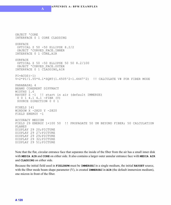
A P P E N D I X A : B P M E X A M P L E SA
OBJECT 'COREINTERFACE 0 1 CORE CLADDING
SURFACE OPTICAL Z 50 -50 ELLIPSE 8.2/2 OBJECT 'CURVED_FACE.INNERINTERFACE 0 1 CORE,AIR
SURFACE OPTICAL Z 50 -50 ELLIPSE 50 50 8.2/100 OBJECT 'CURVED_FACE.OUTERINTERFACE 0 1 CLADDING,AIR
PI=ACOS(-1) V=2*PI/1.55*4.1*SQRT(1.4505^2-1.4447^2) !! CALCULATE V# FOR FIBER MODE
PARABASAL 4BEAMS COHERENT DIFFRACTWIDTHS 1.6RAYSET Z -1 !! start in air (default IMMERSE) 0 0 1 4.1 4.1 -FIBR (V) SOURCE DIRECTION 0 0 1
PIXELS 141WINDOW X -2@20 Y -2@20FIELD ENERGY -1
ACCURACY MEDIUM FIELD 29 ENERGY 1+100 50 !! PROPAGATE 50 UM BEYOND FIBER; 50 CALCULATION PLANESDISPLAY 29 20;PICTUREDISPLAY 29 27;PICTUREDISPLAY 29 29;PICTUREDISPLAY 29 32;PICTURE DISPLAY 29 51;PICTURE
Note that the flat, circular entrance face that separates the inside of the fiber from the air has a small inner disk with MEDIA AIR and CORE on either side. It also contains a larger outer annular entrance face with MEDIA AIR and CLADDING on either side.
Because the initial field used in FIELDBPM must be IMMERSEd in a single medium, the initial RAYSET source, with the fiber mode beam shape parameter (V), is created IMMERSEd in AIR (the default immersion medium), one micron in front of the fiber.
A 120
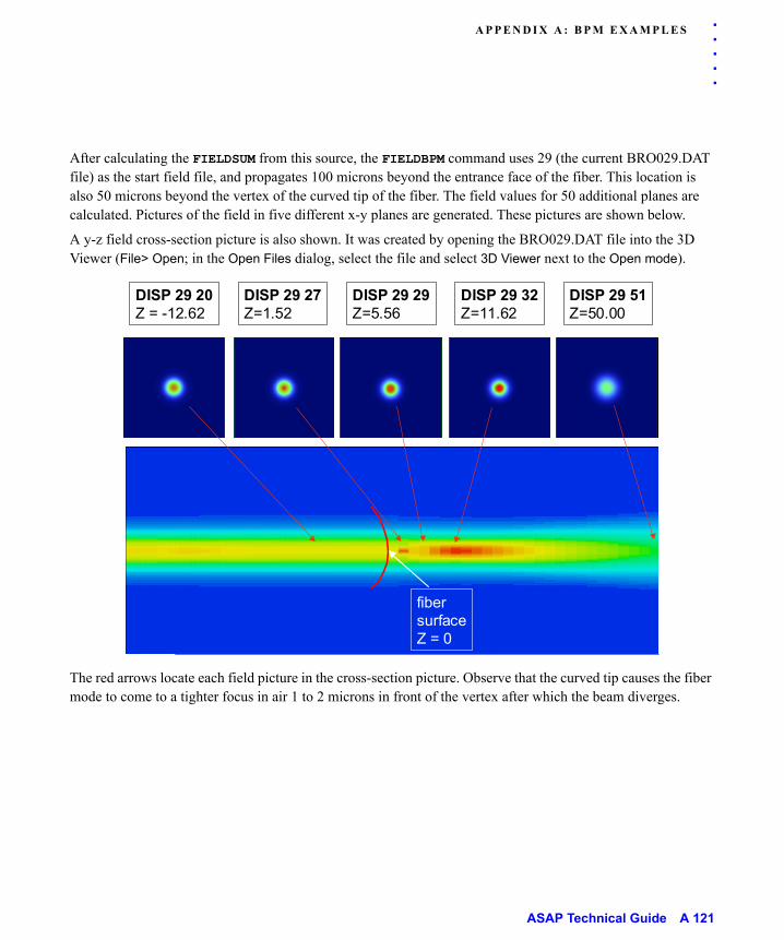
. . .
. .A P P E N D I X A : B P M E X A M P L E S
After calculating the FIELDSUM from this source, the FIELDBPM command uses 29 (the current BRO029.DAT file) as the start field file, and propagates 100 microns beyond the entrance face of the fiber. This location is also 50 microns beyond the vertex of the curved tip of the fiber. The field values for 50 additional planes are calculated. Pictures of the field in five different x-y planes are generated. These pictures are shown below.
A y-z field cross-section picture is also shown. It was created by opening the BRO029.DAT file into the 3D Viewer (File> Open; in the Open Files dialog, select the file and select 3D Viewer next to the Open mode).
The red arrows locate each field picture in the cross-section picture. Observe that the curved tip causes the fiber mode to come to a tighter focus in air 1 to 2 microns in front of the vertex after which the beam diverges.
DISP 29 20Z = -12.62
DISP 29 27Z=1.52
DISP 29 29Z=5.56
DISP 29 32Z=11.62
DISP 29 51Z=50.00
fibersurfaceZ = 0
ASAP Technical Guide A 121
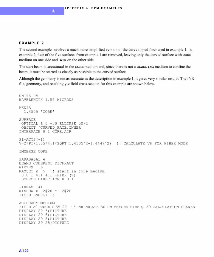
A P P E N D I X A : B P M E X A M P L E SA
E X A M P L E 2
The second example involves a much more simplified version of the curve tipped fiber used in example 1. In example 2, four of the five surfaces from example 1 are removed, leaving only the curved surface with CORE medium on one side and AIR on the other side.
The start beam is IMMERSEd in the CORE medium and, since there is not a CLADDING medium to confine the beam, it must be started as closely as possible to the curved surface.
Although the geometry is not as accurate as the description in example 1, it gives very similar results. The INR file, geometry, and resulting y-z field cross-section for this example are shown below.
UNITS UMWAVELENGTH 1.55 MICRONS
MEDIA 1.4505 'CORE'
SURFACE OPTICAL Z 0 -50 ELLIPSE 50/2 OBJECT 'CURVED_FACE.INNERINTERFACE 0 1 CORE,AIR
PI=ACOS(-1) V=2*PI/1.55*4.1*SQRT(1.4505^2-1.4447^2) !! CALCULATE V# FOR FIBER MODE
IMMERSE CORE
PARABASAL 4BEAMS COHERENT DIFFRACTWIDTHS 1.6RAYSET Z -5 !! start in core medium 0 0 1 4.1 4.1 -FIBR (V) SOURCE DIRECTION 0 0 1
PIXELS 141WINDOW X -2@20 Y -2@20FIELD ENERGY -5
ACCURACY MEDIUM FIELD 29 ENERGY 55 27 !! PROPAGATE 50 UM BEYOND FIBER; 50 CALCULATION PLANESDISPLAY 29 3;PICTUREDISPLAY 29 5;PICTUREDISPLAY 29 8;PICTURE DISPLAY 29 28;PICTURE
A 122
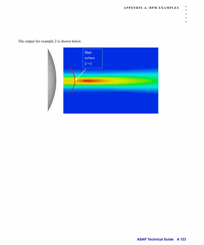
. . .
. .A P P E N D I X A : B P M E X A M P L E S
The output for example 2 is shown below.
fiber
surface
Z = 0
fiber
surface
Z = 0
ASAP Technical Guide A 123
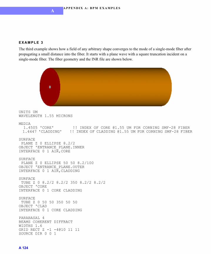
A P P E N D I X A : B P M E X A M P L E SA
E X A M P L E 3
The third example shows how a field of any arbitrary shape converges to the mode of a single-mode fiber after propagating a small distance into the fiber. It starts with a plane wave with a square truncation incident on a single-mode fiber. The fiber geometry and the INR file are shown below.
UNITS UMWAVELENGTH 1.55 MICRONS
MEDIA 1.4505 'CORE' !! INDEX OF CORE @1.55 UM FOR CORNING SMF-28 FIBER 1.4447 'CLADDING' !! INDEX OF CLADDING @1.55 UM FOR CORNING SMF-28 FIBER
SURFACE PLANE Z 0 ELLIPSE 8.2/2OBJECT 'ENTRANCE_PLANE.INNERINTERFACE 0 1 AIR,CORE
SURFACE PLANE Z 0 ELLIPSE 50 50 8.2/100OBJECT 'ENTRANCE_PLANE.OUTERINTERFACE 0 1 AIR,CLADDING
SURFACE TUBE Z 0 8.2/2 8.2/2 350 8.2/2 8.2/2OBJECT 'COREINTERFACE 0 1 CORE CLADDING
SURFACE TUBE Z 0 50 50 350 50 50OBJECT 'CLADINTERFACE 0 1 CORE CLADDING
PARABASAL 4BEAMS COHERENT DIFFRACTWIDTHS 1.6GRID RECT Z -1 -4@10 11 11SOURCE DIR 0 0 1
A 124
. . .
. .A P P E N D I X A : B P M E X A M P L E S
PIXELS 231WINDOW X -2@35 Y -2@35FIELD ENERGY -1
ACCURACY MEDIUM FIELD 29 ENERGY 300 50 !! PROPAGATE 300 UM BEYOND INTO FIBER; 50 CALCULATION PLANESDISPLAY 29 1;PICTUREDISPLAY 29 11;PICTUREDISPLAY 29 21;PICTUREDISPLAY 29 31;PICTUREDISPLAY 29 41;PICTURE DISPLAY 29 51;PICTURE
Like example 1, there is a flat, circular entrance face that separates the inside of the fiber from the air. The entrance face has a small inner disk with MEDIA AIR and CORE on either side and a larger, flat, annular entrance face with MEDIA AIR and CLADDING on either side. The other two surfaces are tubes that define the boundaries between the CORE and CLADDING and the CLADDING and AIR.
Because this example involves propagation ending inside the fiber, it was not necessary to create the geometry for the exit face. The truncated plane wave is created with a GRID source one micron in front of the fiber. After calculating the FIELDSUM from this source, the FIELDBPM command uses 29 (the current BRO029.DAT file) as the start field file, and propagates 300 microns inside the fiber. The field values for 50 additional planes are calculated.
ASAP Technical Guide A 125
A P P E N D I X A : B P M E X A M P L E SA
Pictures of the field in five different x-y planes are generated. These pictures are shown below, along with a y-z field cross-section picture. The red arrows locate each x-y field picture in the cross-section picture.
You can see that, as the beam propagates in z, the portion of the energy that is not needed for the fiber mode escapes the core and gets absorbed due to the default, physically-absorbing boundary conditions. By the end of the propagation, the beam inside the fiber has become that of the correct fiber mode.
DISP 29 11Z = 59
DISP 29 1Z = -1
DISP 29 21Z = 119
DISP 29 31Z = 179
DISP 29 41Z = 239
DISP 29 51Z = 300
DISP 29 11Z = 59
DISP 29 1Z = -1
DISP 29 21Z = 119
DISP 29 31Z = 179
DISP 29 41Z = 239
DISP 29 51Z = 300
A 126
. . .
. .A P P E N D I X A : B P M E X A M P L E S
E X A M P L E 4
The fourth example demonstrates how to generate the field emerging from a single-mode fiber that has its exit face cleaved at an 8-degree angle. The fiber geometry and the INR file are shown below.
SYSTEM NEWRESET
UNITS UMWAVELENGTH 1.55 MICRONS
MEDIA 1.4505 'CORE' 1.4447 'CLADDING' SURFACE PLANE Z 0 ELLIPSE 8.2/2OBJECT 'FIBER.INNER1'INTERFACE 0 1 AIR,CORE
SURFACE PLANE Z 0 ELLIPSE 125/2 125/2 8.2/125OBJECT 'FIBER.OUTER1'INTERFACE 0 1 AIR,CLADDING
SURFACE PLANE Z 20 ROTATE X 8 0 20 TUBE Z 0 8.2/2 8.2/2 50 8.2/2 8.2/2OBJECT 'FIBER.CORE_TUBE' INTERFACE 0 1 CORE CLADDING BOUNDS -.2
ASAP Technical Guide A 127
A P P E N D I X A : B P M E X A M P L E SA
SURFACE PLANE Z 20 ROTATE X 8 0 20 TUBE Z 0 125/2 125/2 50 125/2 125/2OBJECT 'FIBER.CLAD_TUBE' INTERFACE 0 1 CLADDING AIR BOUNDS -.2
SURFACE PLANE Z 20 ELLIPSE 8.2/2 ROTATE X 8 0 20 OBJECT 'FIBER.INNER2'INTERFACE 0 1 CORE,AIR
SURFACE PLANE Z 20 ELLIPSE 125/2 125/2 8.2/125 ROTATE X 8 0 20 OBJECT 'FIBER.OUTER2'INTERFACE 0 1 CLADDING,AIR
RAYSET Z -.0001 0 0 1 4.1 4.1 -9 2.1537SOURCE DIRECTION 0 0 1
PIXELS 141WINDOW Y -2@20 X -2@20 FIELD ENERGY -.0001
ACCURACY LOW FIELD 29 ENERGY 60DISPLAY ;PICTURE
Once again, there is a flat, circular entrance face that separates the inside of the fiber from the air. The entrance face has a small inner disk with MEDIA AIR and CORE on either side, and a larger flat annular entrance face with MEDIA AIR and CLADDING on either side. Other surfaces include tubes that define the boundaries between the CORE and CLADDING and CLADDING and AIR; and a flat, elliptical, exit face, which is identical to the entrance face except that it is tilted by eight degrees.
A 128
. . .
. .A P P E N D I X A : B P M E X A M P L E S
A fundamental fiber mode source is created a small fraction of a micron in front of the fiber. After calculating the FIELDSUM from this source, the FIELDBPM command uses 29 (the current BRO029.DAT file) as the start field file, and propagates to a plane approximately 40 microns beyond the exit face of the fiber. The picture of this field below shows that the beam radius has expanded slightly to a 1/e2 value of 6.6 microns, and the beam center is shifted by about 2 microns in the y direction due to the 8-degree cleave.
There is a simpler way to generate a nearly identical result where there are only two surfaces and one medium, as shown in the INR file below.
SYSTEM NEWRESET
UNITS UMWAVELENGTH 1.55 UM
MEDIA 1.4505 'CORE'
SURFACE PLANE Z 0 ELLIP 125/2 125/(2*COS[8]) ROTATE X 8 0 0
ASAP Technical Guide A 129
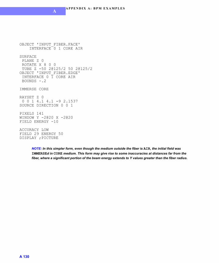
A P P E N D I X A : B P M E X A M P L E SA
OBJECT 'INPUT_FIBER.FACE' INTERFACE 0 1 CORE AIR
SURFACE PLANE Z 0 ROTATE X 8 0 0 TUBE Z -50 2@125/2 50 2@125/2 OBJECT 'INPUT_FIBER.EDGE' INTERFACE 0 1 CORE AIR BOUNDS -.2
IMMERSE CORE
RAYSET Z 0 0 0 1 4.1 4.1 -9 2.1537SOURCE DIRECTION 0 0 1
PIXELS 141WINDOW Y -2@20 X -2@20 FIELD ENERGY -10
ACCURACY LOW FIELD 29 ENERGY 50 DISPLAY ;PICTURE
NOTE: In this simpler form, even though the medium outside the fiber is AIR, the initial field was
IMMERSEd in CORE medium. This form may give rise to some inaccuracies at distances far from the
fiber, where a significant portion of the beam energy extends to Y values greater than the fiber radius.
A 130


![Gaussian Beam Optics [Hecht Ch. pages 594 596 … Beam Optics [Hecht Ch. 13.1 pages 594596 Notes from Melles Griot and Newport] Readings: For details on the theory of Gaussian beam](https://static.documents.pub/doc/80x56/5ab6c9d67f8b9a2f438e0d48/gaussian-beam-optics-hecht-ch-pages-594-596-beam-optics-hecht-ch-131-pages.jpg)


