WEALTH BIAS IN THE FIRST GLOBAL CAPITAL MARKET BOOM, 1870-1913

by

Michael A. ClemensJeffrey G. WilliamsonHarvard University

July 2001

This study would not have been possible without the generosity of Irving Stone, who supplied detailed informationdocumenting British foreign investment that was not published in his book. We are also grateful to Robert Allen, ChrisMeissner and Luís Bertola who kindly provided some of their unpublished data. The authors thank John Baldiserotto, XimenaClark, John Collins, David Foster, Heather McMullen, Ann Richards, and Danila Terpanjian for their excellent researchassistance. We have benefited from extended discussions with Francesco Caselli and Andrew Warner, as well as fromcomments by Michael Bordo, John Coatsworth, Daniel Devroye, Scott Eddie, Barry Eichengreen, David Good, Yael Hadass,Matt Higgins, Macartan Humphreys, John Komlos, Michael Kremer, Philip Kuhn, Deirdre McCloskey, Chris Meissner,Kevin O�Rourke, Ken Rogoff, Matt Rosenberg, Dick Salvucci, Howard Shatz, Max Schulze, Alan Taylor, Yishay Yafeh andparticipants at the May 2001 Cliometrics Conference. Remaining errors belong to us. Williamson acknowledges with pleasurefinancial support from the National Science Foundation SES-0001362, and both authors thank the Center for InternationalDevelopment for allocating office space to the project.

Abstract

Why do rich countries receive the lion�s share of international investment flows? Though this wealthbias is strong today, it was even stronger during the first great global capital market boom, after 1870.Very little of British capital exports went to poor, labor-abundant countries. Indeed, only about a quarterwent to labor-abundant Asia and Africa where almost two-thirds of the world�s population lived, whileabout two-thirds went to the labor-scarce New World where only a tenth of the world�s population lived. Was this geographic distribution of capital flows caused by some international capital market failure, orwas it due to a shortfall in underlying economic, demographic or geographic fundamentals thatdiminished the productivity of capital in poor countries? This paper constructs a panel data set for 34countries that as a group received 92% of British capital, and uses it to conclude that international capitalmarket failure (including whether the country was on or off the Gold Standard) had only second-ordereffects on the geographical distribution of British capital. It then ranks the three big fundamentals thatmattered most�schooling, natural resources and demography.

JEL No. F21, N20, O1

Michael A. Clemens Jeffrey G. WilliamsonDepartment of Economics Department of EconomicsHarvard University Harvard UniversityCambridge, MA 02138 Cambridge MA 02138and Center for International Development and NBER and Center formclemens@fas.harvard.edu International Development

jwilliam@kuznets.harvard.edu

1

I. Introduction

Rich countries receive the lion�s share of cross-border investment. A large literature has

proposed theoretical explanations for this wealth bias (Barro 1989; King and Rebelo 1989; Gertler and

Rogoff 1990; Lucas 1990; and others since), but exploration of the wealth bias during the first great

global capital boom, after 1870, has only just begun (Lane and Milesi-Ferretti 1999; Kohl and O�Rourke

2000; Obstfeld and Taylor 2001). It appears, in fact, that no study has yet investigated the determinants

of the geographic distribution of international investment before World War I.

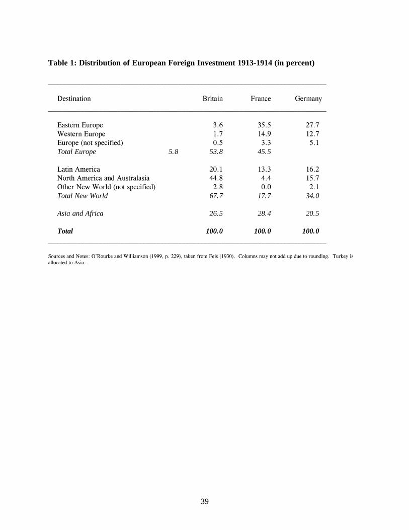
Table 1 summarizes the destination of European foreign investment just prior to World War I,

and very little of it went to poor, capital-scarce and labor-abundant countries.1 Indeed, only about a

quarter of British foreign investment went to labor-abundant Asia and Africa where almost two-thirds of

the world�s population lived, while about two-thirds went to the labor-scarce New World where only a

tenth of the world�s population lived. The simplest explanation of this bias is that British capital chased

after European emigrants and that both were seeking cheap land and other natural resources (O�Rourke

and Williamson 1999, Chap. 12), although Table 1 shows that French and German capital did not chase

after the emigrants heading to the New World anywhere near as much as did the British. While French

and German capital preferred European to New World opportunities, the same small capital export

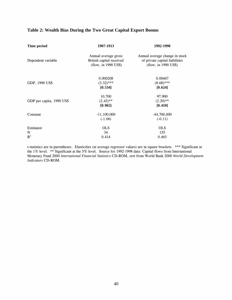
shares went to Asia and Africa.2 Furthermore, Table 2 suggests that the wealth bias was even stronger

before World War I than it is today since the elasticity of foreign capital received with respect to GDP

per capita was almost twice as big then as now.3

The venerable capital-chased-after-labor explanation argues that there must have been an omitted

variable at work, and most economic observers of the late 19th century would say that it was natural

1 Almost thirty years ago one economic historian used some of the same data used here (only for five New Worldcountries: Argentina, Australia, Canada, New Zealand, United States) and concluded that GDP was the onlyvariable that consistently predicted British capital distribution (Richardson 1972, p. 109).2 We have not been able to secure the same kind of panel data for France and Germany in the four decades prior toWorld War I. Too bad, since we�d like to know whether French and German investors obeyed the same laws ofmotion that characterized British investors, even though the latter favored the New World over Europe.

2

resources. In contrast, most economic observers of the late 20th century would say it was human

capital. But surely the phenomenon deserves more serious attention than that offered by some mono-

causal natural resource or human capital endowment explanation. Furthermore, we want to sort out what

role policy and institutions played in the process�like the Gold Standard�after we have controlled for

the economic, demographic and political fundamentals. Finally, we hope to combine this study of late

19th century British investment abroad with a similar study of late 20th century United States investment

abroad (Clemens ongoing) to learn how the determinants of the wealth bias have changed with time.

The debate over the cause of the wealth bias breaks down into two camps: those who believe that

capital is in fact highly productive in poor countries but does not flow there due to failures in the global

financial capital market or in the global capital goods market, and those who believe that capital would

not be very productive in poor countries even with perfect capital markets and thus has no reason to flow

there. We refer to the first claim as the global capital market failure view, and the second as the

unproductive domestic capital view.

II. Potential Explanations for the Wealth Bias: A Review of the Literature

The Global Capital Market Failure4 View

Studies positing that the wealth bias can be explained by failure in a competitive international

capital market invite the following organization. The demand for foreign savings can be choked off by

domestic tariffs, distance from source, and other distortions that yield wide user cost differentials

between countries even where financial costs are equalized. The supply of foreign savings can be

deflected by other global capital market failures, like adverse selection, herding, the absence of a stable

monetary standard, and colonial intervention through the application of force. Each will be discussed in

turn.

3 Also note that the elasticity on market size (e.g. GDP) was smaller in 1907-1913 than it is today.

3

Tariffs, Distance from London and Other Distortions. Matthew Higgins (1993; summarized in

Taylor 1998) demonstrates that after correcting for higher prices of capital goods, much of the incentive

to invest in many contemporary less developed countries (LDCs) evaporates. Empirical work by Charles

Jones (1994) on the years following 1950, and William Collins and Jeffrey Williamson (2001) on the

years before 1950, extend the work of J. Bradford DeLong and Lawrence Summers (1991) to show that

distortions in equipment prices significantly depress domestic investment as well as growth. What

distortion might prevent the capital market from sending enough financial capital to poor countries where

the marginal product of capital is high? The idea that tariffs on manufactures early in industrial

development could deter foreign capital inflows is as old as List (1856, pp. 227, 314) and Pigou (1906,

p.11).5 Citing the example of Argentina after the 1930s, Alan Taylor (1998) shows how import

substitution policies�and their accompanying price distortions�stifled capital flows (and accumulation)

even when the undistorted marginal product of capital was high. High transportation costs or distance

from London might do the same.

Adverse Selection and Costly State Verification. Applying asymmetric information theories,

several authors have argued that the international credit market is rationed by adverse selection and

costly state verification (e.g. Boyd and Smith 1992; Gordon and Bovenberg 1996; Razin, Sadka and

Yuen 1999; Hanson 1999). That is, wealthy investors will not accept the high returns to capital available

in developing countries because the presence of that capital may attract high-risk borrowers, creating

potential losses which exceed the gains due to otherwise outstanding investment opportunities.

Herding and the Foreign Bias. One of the older hypotheses used to explain Victorian and

Edwardian Britain�s economic slowdown was that the City of London had an irrational foreign bias,

systematically discriminated against domestic borrowers, starved the home industry for funds, and

contributed to an accumulation slowdown. According to this thesis, market failure at home accounted

4 We define “market failure” as that which occurs “when the allocations achieved with markets are not efficient”(Eatwell et al., 1987), for any reason. Thus what some refer to as “government failure,” we call “market failure.”5 O�Rourke (2000) provides evidence that protective tariffs raised TFP before WW1 in ten economies moreadvanced in their industrialization, just as List said it would.

4

for the huge capital export from Britain (O�Rourke and Williamson 1999, p. 226). Evidence offered by

Michael Edelstein (1976, 1981, 1982) certainly did grave damage to the thesis, but it may still have

power in accounting for the heavy preference for New World investment. After all, this foreign capital

export boom seems to be characterized by the same attributes theorists assign to herding behavior in

financial capital markets today (Banerjee 1992; Cont and Bouchaud 2000).

Stable Monetary Systems. The global economy was dominated by the Gold Standard after the

1870s, and many observers argue that it promoted international capital mobility by eliminating exchange

risk (Eichengreen 1996). Others argue that the Gold Standard commitment provided an investor

guarantee that the country in question would pursue conservative fiscal and monetary policies (Bordo and

Kydland 1995; Bordo and Rockoff 1996), policies that would make potential investors more willing to

risk their capital overseas. While the argument certainly seems plausible, it is, of course, possible that

the Gold Standard policy choice and the foreign capital inflow were both determined by more

fundamental influences. Barry Eichengreen (1992) has persuasively argued the case for these political

and economic fundamentals, a position taken some time ago by Karl Polanyi (1944) and restated in

modern economic language recently by Maurice Obstfeld and Taylor (1998).

Colonial Intervention. Late 19th century colonial intervention (plus gun-boat diplomacy) created

a friendly environment for international lending, or so says a very large literature. After controlling for

other things that mattered to investors, did British foreign capital follow the flag or follow the market?

The Unproductive Domestic Capital View

The alternative view of the wealth bias is to explain it by appealing to absent third factors. This

unproductive domestic capital view actually assumes perfect financial capital markets, although it

stresses that there may be failures in other markets that might impact on this one. The supply of foreign

capital may be cut back by positive correlations of business cycles between developed and developing

countries, since wealthy-country investors seek both high average returns and insurance against financial

5

disaster that a diversified portfolio offers. The demand for international investment can be choked off by

limitations on internationally immobile third factors such as schooling, skills, natural resources,

demographic factors, unenforceable property rights, and what has come to be called social capital

(Putnam 1995; Glaeser et al. 2000).

Business Cycle and Long Swing Correlations. Several economists (Cox et al. 1985; Tobin

1992; Bohn and Tesar 1996) have sought to explain gross (rather than net) capital flows by the increased

supply of foreign capital available to countries with business cycles uncorrelated or, even better,

inversely correlated with that of the host country, allowing portfolio diversification for investors in the

latter. This theoretical view will find a comfortable haven in history since the inverse pre-1913

correlation between British domestic investment and capital exports has long been appreciated by

economic historians (Cairncross 1953; Thomas 1954; Williamson 1964; Abramovitz 1968). Perhaps this

correlation also played a role in influencing the direction taken by British foreign capital.

Third Factors: Natural Resources, Skills and Schooling. Consider a neoclassical production

function Y = AKαLβSγ, where S is some third factor and there are constant returns (α + β + γ = 1). The

marginal product of capital YK and the marginal product of labor YL are

γα−β

γβ−α

β=

α=

SKLAY

SLKAY1

L

1K

It is easy to see that low marginal products of capital and low marginal products of labor can coexist�

provided the country is sufficiently poor in S.

Economic historians would be quick to offer a candidate for this immobile third factor role�

natural resources, and David Bloom and Jeffrey Sachs (1998) have argued the same case when looking

for explanations of African performance more recently. It has a venerable tradition in economic

history,6 and we will give that tradition plenty of scope to influence the empirical results later in this

paper.

6 The literature is large. See, for example, Cairncross 1953; DiTella 1982; Green and Urquhart 1976; Kuznets

6

Robert Lucas (1990) took the view that the immobile third factor was human capital�skills and

schooling. While there are reasons to suppose that human capital was much less central to the growth

process in the 19th than in the 20th century, Gabriel Tortella (1994) has effectively argued the contrary

to help account for Iberian backwardness. Kevin O�Rourke (1992) has done the same for Ireland: if Irish

workers with the greatest human capital endowments self-selected for emigration, capital�s marginal

product would have fallen in 19th century Ireland, thus choking off capital flows from Britain. Similarly,

the work of Gregory Clark (1987) shows enormous differences in the profitability of cotton textile mills

across the globe just before World War I, and cheap labor did not help poor countries much since labor

was not very productive. However, Clark thinks that cultural forces reduced worker productivity in poor

countries, not the absence of skills and schooling.

Third Factors: Demography. The dependency ratio, defined as the percentage of the population

not engaged in productive activities (whether remunerated or not), is typically viewed as an immobile

characteristic of a country�s labor force. It increases in response to baby booms, improved child

survival rates and adult longevity, although the latter was a minor event in the 19th century. It decreases

in response to an inflow of working-age immigrants. Assuming that dependents affect a household�s

ability to save and that labor force participation affects productivity and therefore investment,

dependency rates have the potential to impact capital flows. Demographic models like those of Higgins

and Williamson (1997) and Bloom and Williamson (1998) show how changes in the demographic

structure can matter. As the country develops, the demographic transition to a lower youth dependency

burden and a more mature adult population increases the productivity of both the population and the

labor force. Further development, of course, can reverse the effect as the elderly dependency burden

rises.

In order for the demographic structure to affect capital flows, it must have differential effects on

investment and savings. Its effect on investment is clear from the simple third factor equations above:

1958; O�Rourke and Williamson 1999, Chap. 12.

7

lower youth dependency and higher adult participation rates means a higher marginal product of capital,

which, in turn, implies more investment demand. And more investment demand implies more demand

for foreign capital unless domestic savings increases. The domestic saving response to a change in the

dependency burden is, however, less clear as those who have followed the life cycle debate will

appreciate. Guided by previous work using late 19th century evidence (Taylor and Williamson 1994), we

expect the dependency rate to play a role in determining capital flows, young populations being more

dependent on foreign capital.7

Third Factors: Unenforceable Property Rights. Even if an investor can easily prove

noncompliance to an investment contract, this information is of little use if the enforcement mechanism is

inadequate or, even worse, non-existent. Thus, foreign investment will not take place in potential-

borrowing countries where contract enforcement and property rights are absent, and wide differences in

the marginal product of capital can exist. Contracts may be unenforceable due to the absence of needed

judiciary and executive public institutions, both at the national and international level. Aarón Tornell and

Andrés Velasco (1992) proposed just such an explanation for low capital flows to poor countries.

Sometimes these capital flows can even be negative, as in Cecil Rhodes� Africa, when rents from mines

underwent capital flight to rich countries where returns were low but property rights were enforced by

law rather than by gunpowder and steel. Riccardo Faini (1996) offers another example: labor mobility

out of countries with low capital stocks toward those with high capital stocks (and thus high wages) can

by depopulation keep the marginal product of capital low even in countries with low capital. Since labor

cannot be used as collateral for loans, these countries cannot borrow against their labor force to build

sufficient physical capital stocks to prevent the emigration.

Third Factors: Geography and Others. There are other candidates for the third factor role. In

their recent effort to reclaim the importance of geography on recent economic performance, Bloom and

Sachs (1998) stress distance from periphery to core, a factor which is likely to have been even more

7 This prediction has been confirmed with late 20th century evidence (Higgins and Williamson 1997).

8

important in the 19th century when distance had a bigger impact on cost. Helmut Reisen (1994) has

explicitly pointed to the potential role of geographic distance to neighboring markets and urban

agglomerations on capital flows. The seminal industrial organization theories of Raymond Vernon (1966)

and Stephen Hymer (1976) fall into this category as well; their vision of scale effects, managerial

knowledge, distribution networks, product cycles and other firm-specific intangibles can all be modeled

as immobile third factors affecting the marginal product of capital. Others have explored yet another

immobile third factor�specialized, nontraded intermediate inputs.

It is very clear that there is no shortage of theoretical assertions to motivate empirical analysis.

What�s missing in the wealth bias literature, however, is empirical analysis. In this regard, economic

history has much to offer.

III. A Simple Model: Testable Predictions of the Two Views

This exposition uses the standard Ramsey open-economy growth model, recently formalized by

Robert Barro and Xavier Sala-i-Martín (1995), to motivate the regression specifications found in Section

IV. We begin by holding to the initial assumptions made by Lucas (1990): two factors and no capital

market imperfections. Like Lucas, we show that the wealth bias can be explained by relaxing either of

these assumptions. We go on to derive which empirically testable conditions are necessary for either

explanation to be correct.

The Wealth Bias

Let Yi represent the output of country i, Ki represent the stock of capital in country i, and Li

represent the population of country i. The lower case yi and ki signify per capita output and per capita

capital stock, respectively, and yi = Aif(ki) where Ai is the level of technology or total factor productivity

in country i. The function f is neoclassical (i.e. f(0) = 0, f ’ > 0, and f ” < 0). For the simplest

9

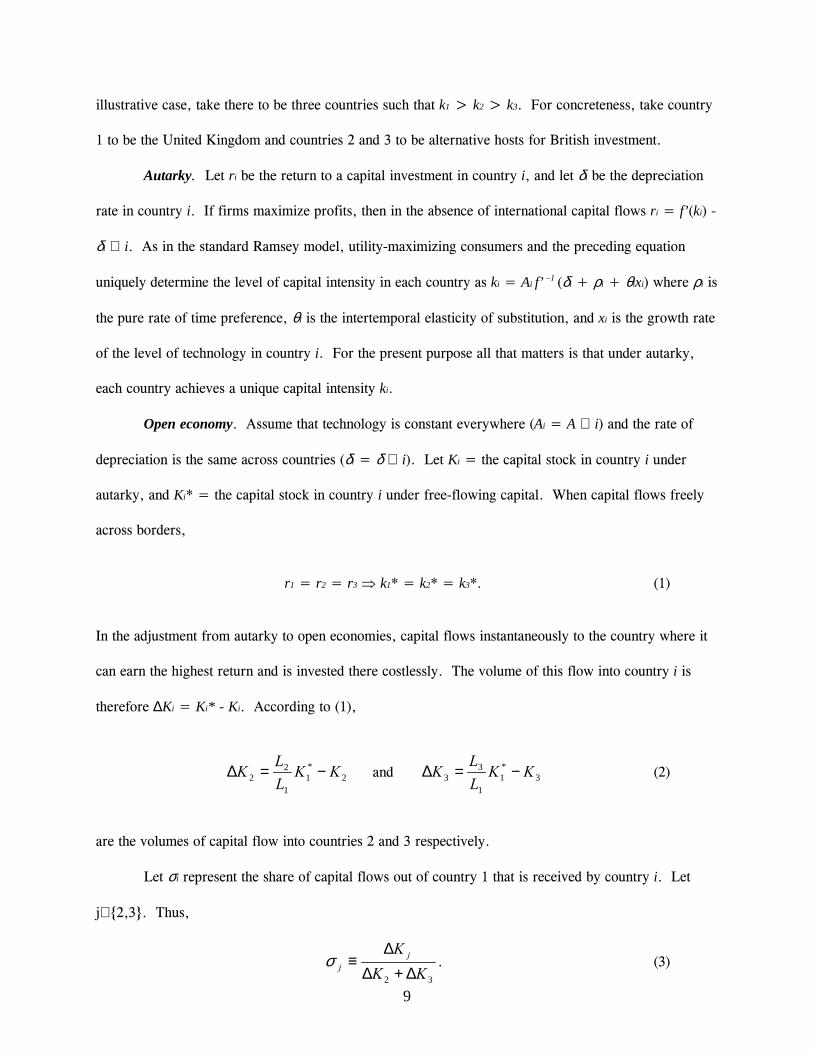
illustrative case, take there to be three countries such that k1 > k2 > k3. For concreteness, take country

1 to be the United Kingdom and countries 2 and 3 to be alternative hosts for British investment.

Autarky. Let ri be the return to a capital investment in country i, and let δi be the depreciation

rate in country i. If firms maximize profits, then in the absence of international capital flows ri = f’(ki) -

δi ∀ i. As in the standard Ramsey model, utility-maximizing consumers and the preceding equation

uniquely determine the level of capital intensity in each country as ki = Ai f’ –1 (δi + ρi + θixi) where ρi is

the pure rate of time preference, θi is the intertemporal elasticity of substitution, and xi is the growth rate

of the level of technology in country i. For the present purpose all that matters is that under autarky,

each country achieves a unique capital intensity ki.

Open economy. Assume that technology is constant everywhere (Ai = A ∀ i) and the rate of

depreciation is the same across countries (δi = δ ∀ i). Let Ki = the capital stock in country i under

autarky, and Ki* = the capital stock in country i under free-flowing capital. When capital flows freely

across borders,

r1 = r2 = r3 ⇒ k1* = k2* = k3*. (1)

In the adjustment from autarky to open economies, capital flows instantaneously to the country where it

can earn the highest return and is invested there costlessly. The volume of this flow into country i is

therefore ∆Ki = Ki* - Ki. According to (1),

2*1

1

22 KK

LLK −=∆ and 3

*1

1

33 KK

LL

K −=∆ (2)

are the volumes of capital flow into countries 2 and 3 respectively.

Let σi represent the share of capital flows out of country 1 that is received by country i. Let

j∈ {2,3}. Thus,

32 KKK j

j ∆+∆∆

≡σ . (3)

10

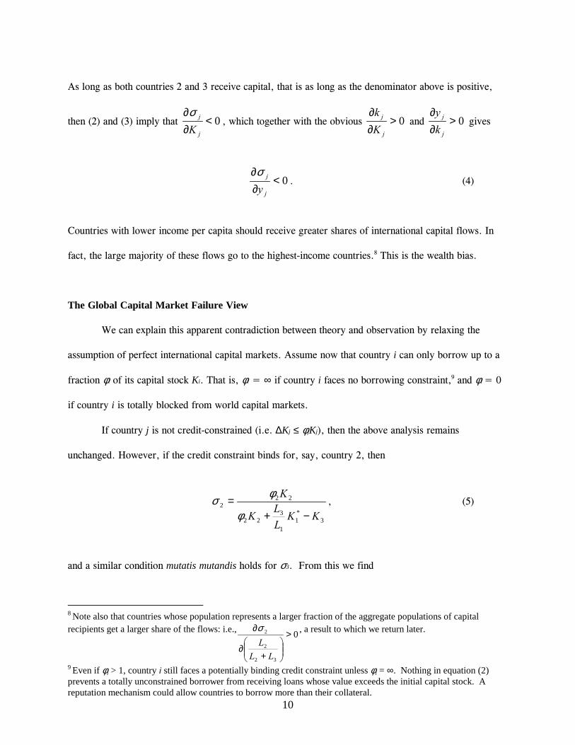
As long as both countries 2 and 3 receive capital, that is as long as the denominator above is positive,

then (2) and (3) imply that 0<∂∂

j

j

Kσ

, which together with the obvious 0>∂∂

j

j

Kk

and 0>∂∂

j

j

ky

gives

0<∂∂

j

j

yσ

. (4)

Countries with lower income per capita should receive greater shares of international capital flows. In

fact, the large majority of these flows go to the highest-income countries.8 This is the wealth bias.

The Global Capital Market Failure View

We can explain this apparent contradiction between theory and observation by relaxing the

assumption of perfect international capital markets. Assume now that country i can only borrow up to a

fraction φi of its capital stock Ki. That is, φi = ∞ if country i faces no borrowing constraint,9 and φi = 0

if country i is totally blocked from world capital markets.

If country j is not credit-constrained (i.e. ∆Kj ≤ φjKj), then the above analysis remains

unchanged. However, if the credit constraint binds for, say, country 2, then

3*1

1

322

222

KKLLK

K

−+=

φ

φσ , (5)

and a similar condition mutatis mutandis holds for σ3. From this we find

8 Note also that countries whose population represents a larger fraction of the aggregate populations of capitalrecipients get a larger share of the flows: i.e., 0

32

2

2 >

+

∂

∂

LLLσ , a result to which we return later.

9 Even if φi > 1, country i still faces a potentially binding credit constraint unless φi = ∞. Nothing in equation (2)prevents a totally unconstrained borrower from receiving loans whose value exceeds the initial capital stock. Areputation mechanism could allow countries to borrow more than their collateral.

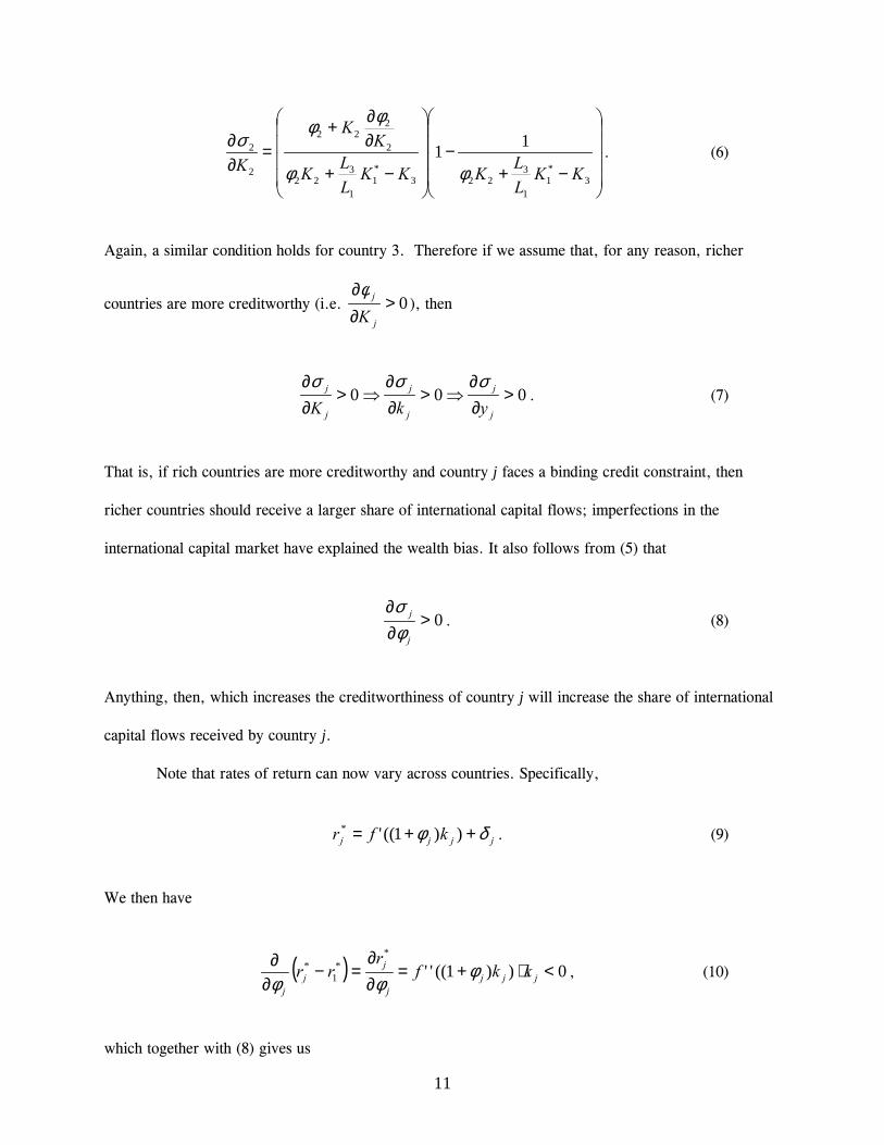
11

−+−

−+

∂∂+

=∂∂

3*1

1

3223

*1

1

322

2

222

2

2 11KK

LLKKK

LLK

KK

K φφ

φφσ

. (6)

Again, a similar condition holds for country 3. Therefore if we assume that, for any reason, richer

countries are more creditworthy (i.e. 0>∂∂

j

j

Kφ

), then

000 >∂∂

⇒>∂∂

⇒>∂∂

j

j

j

j

j

j

ykKσσσ

. (7)

That is, if rich countries are more creditworthy and country j faces a binding credit constraint, then

richer countries should receive a larger share of international capital flows; imperfections in the

international capital market have explained the wealth bias. It also follows from (5) that

0>∂∂

j

j

φσ

. (8)

Anything, then, which increases the creditworthiness of country j will increase the share of international

capital flows received by country j.

Note that rates of return can now vary across countries. Specifically,

jjjj kfr δφ ++= ))1(('* . (9)

We then have

( ) 0))1((''*

*1

* <⋅+=∂∂

=−∂∂

jjjj

jj

j

kkfr

rr φφφ

, (10)

which together with (8) gives us

12

0)( *

1* <

−∂∂

rrjjσ

. (11)

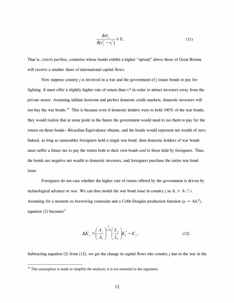
That is, ceteris paribus, countries whose bonds exhibit a higher �spread� above those of Great Britain

will receive a smaller share of international capital flows.

Now suppose country j is involved in a war and the government of j issues bonds to pay for

fighting. It must offer a slightly higher rate of return than rj* in order to attract investors away from the

private sector. Assuming infinite horizons and perfect domestic credit markets, domestic investors will

not buy the war bonds.10 This is because even if domestic lenders were to hold 100% of the war bonds,

they would realize that at some point in the future the government would need to tax them to pay for the

return on those bonds�Ricardian Equivalence obtains, and the bonds would represent net wealth of zero.

Indeed, as long as (untaxable) foreigners hold a single war bond, then domestic holders of war bonds

must suffer a future tax to pay the return both to their own bonds and to those held by foreigners. Thus,

the bonds are negative net wealth to domestic investors, and foreigners purchase the entire war bond

issue.

Foreigners do not care whether the higher rate of return offered by the government is driven by

technological advance or war. We can thus model the war bond issue in country j as Aj > Ai ∀ i.

Assuming for a moment no borrowing constraint and a Cobb-Douglas production function (yi = Aikiα),

equation (2) becomes11

jjj

j KKLL

AA

K −

=∆

−*1

1

11

1

α. (12)

Subtracting equation (2) from (12), we get the change in capital flows into country j due to the war in the

10 This assumption is made to simplify the analysis; it is not essential to the argument.

13

absence of credit constraints:

∆Kj, war - ∆ Kj, no war = 01 *1

1

11

1

>

−

−K

LL

AA jj

α. (13)

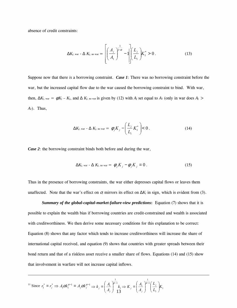
Suppose now that there is a borrowing constraint. Case 1: There was no borrowing constraint before the

war, but the increased capital flow due to the war caused the borrowing constraint to bind. With war,

then, ∆Kj, war = φjKj � Kj, and ∆ Kj, no war is given by (12) with Aj set equal to A1 (only in war does Aj >

A1). Thus,

∆Kj, war - ∆ Kj, no war = 0*1

1

<

− KLL

K jjjφ . (14)

Case 2: the borrowing constraint binds both before and during the war,

∆Kj, war - ∆ Kj, no war = 0=− jjjj KK φφ . (15)

Thus in the presence of borrowing constraints, the war either depresses capital flows or leaves them

unaffected. Note that the war�s effect on σj mirrors its effect on ∆Kj in sign, which is evident from (3).

Summary of the global-capital-market-failure-view predictions: Equation (7) shows that it is

possible to explain the wealth bias if borrowing countries are credit-constrained and wealth is associated

with creditworthiness. We then derive some necessary conditions for this explanation to be correct:

Equation (8) shows that any factor which tends to increase creditworthiness will increase the share of

international capital received, and equation (9) shows that countries with greater spreads between their

bond return and that of a riskless asset receive a smaller share of flows. Equations (14) and (15) show

that involvement in warfare will not increase capital inflows.

11 Since 1111

**1

−− =⇒= αα αα jjj kAkArr1

11

1 kAAkj

j

−

=⇒

α

11

11

1 KLL

AAK j

jj

=⇒

−α

14

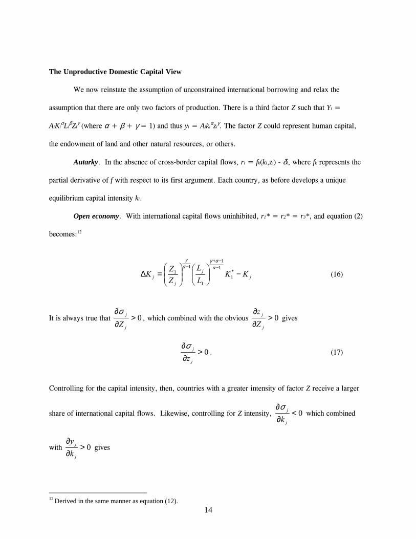
The Unproductive Domestic Capital View

We now reinstate the assumption of unconstrained international borrowing and relax the

assumption that there are only two factors of production. There is a third factor Z such that Yi =

AiKiαLi

βZiγ (where α + β + γ = 1) and thus yi = Aiki

αziγ. The factor Z could represent human capital,

the endowment of land and other natural resources, or others.

Autarky. In the absence of cross-border capital flows, ri = fk(ki,zi) - δi, where fk represents the

partial derivative of f with respect to its first argument. Each country, as before develops a unique

equilibrium capital intensity ki.

Open economy. With international capital flows uninhibited, r1* = r2* = r3*, and equation (2)

becomes:12

jj

jj KK

LL

ZZK −

=∆

−−+

−*1

11

1

11

ααγ

αγ

(16)

It is always true that 0>∂∂

j

j

Zσ

, which combined with the obvious 0>∂∂

j

j

Zz

gives

0>∂∂

j

j

zσ

. (17)

Controlling for the capital intensity, then, countries with a greater intensity of factor Z receive a larger

share of international capital flows. Likewise, controlling for Z intensity, 0<∂∂

j

j

kσ

which combined

with 0>∂∂

j

j

ky

gives

12 Derived in the same manner as equation (12).

15

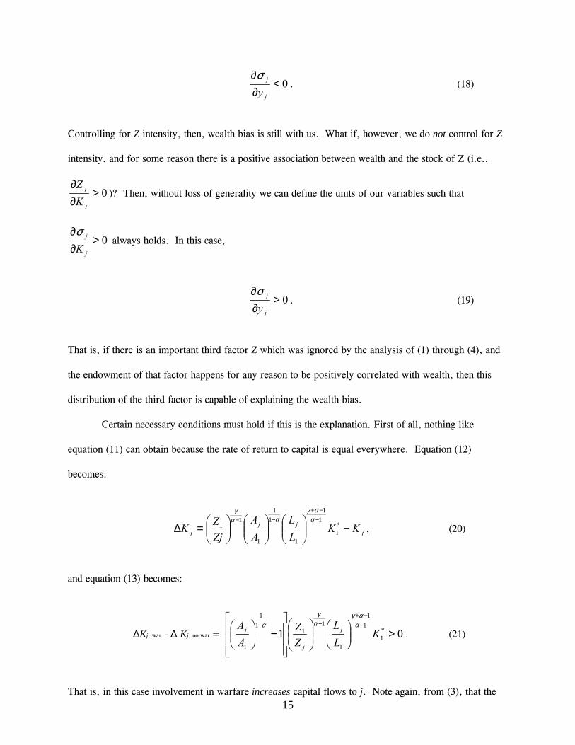
0<∂∂

j

j

yσ

. (18)

Controlling for Z intensity, then, wealth bias is still with us. What if, however, we do not control for Z

intensity, and for some reason there is a positive association between wealth and the stock of Z (i.e.,

0>∂∂

j

j

KZ

)? Then, without loss of generality we can define the units of our variables such that

0>∂∂

j

j

Kσ

always holds. In this case,

0>∂∂

j

j

yσ

. (19)

That is, if there is an important third factor Z which was ignored by the analysis of (1) through (4), and

the endowment of that factor happens for any reason to be positively correlated with wealth, then this

distribution of the third factor is capable of explaining the wealth bias.

Certain necessary conditions must hold if this is the explanation. First of all, nothing like

equation (11) can obtain because the rate of return to capital is equal everywhere. Equation (12)

becomes:

jjj

j KKLL

AA

ZjZK −

=∆−

−+−−

*1

11

1

11

1

11

ααγ

ααγ

, (20)

and equation (13) becomes:

∆Kj, war - ∆ Kj, no war = 01 *1

11

1

11

11

1

>

−

−−+

−−K

LL

ZZ

AA j

j

jα

αγα

γα

. (21)

That is, in this case involvement in warfare increases capital flows to j. Note again, from (3), that the

16

war�s effect on σj has the same sign as its effect on ∆Kj.

Summary of the unproductive-domestic-capital-view predictions: Equation (19) shows that it is

possible to the explain wealth bias with the presence of some previously-omitted third factor of

production. Equation (17) shows that a greater intensity of the third factor encourages capital flows, and

equation (21) shows that involvement in warfare likewise encourages capital flows.

IV. Testing the Theory: What Explains the Wealth Bias in British Capital Exports?

To the degree that return-maximizing international investors were attracted to or deterred from

countries with fundamental national characteristics which affected in equal measure the returns to

national or international investors, we can reject the global capital market failure view.13 To be precise,

we say that the market for British capital exports exhibits the wealth bias when countries with higher

GDP per capita�controlling only for log GDP�receive a significantly larger share of total British

capital exports than do countries with lower GDP per capita. We say that we �explain� the wealth bias

when variables representing country fundamentals and market failure have a statistically significant effect

on British capital inflows and GDP per capita loses its positive significance.

We turn now to the behavior of British overseas investors during the first great globalization

boom between 1870 and 1913.14 British foreign investment is selected for two reasons. First, the British

evidence is available, and it is not for other capital exporters. Second, Britain was then the world�s

leading capital exporter, far exceeding the combined capital exports of its nearest competitors, France

and Germany (Feis 1930, pp. xix-xxi, 71). The keystone of our analysis is the data on gross British

13 Remember that this view posits international capital market failure rather than domestic capital market failure;the latter implies unproductive capital for investors of all flags. Note also that the converse of our test is not true.That is, while the determination of flows by fundamental national characteristics is sufficient to reject the capitalmarket failure view, lack of such determination is merely a necessary condition to reject the unproductive capitalview.14 Certainly Britain (and others) exported capital before this period, as studied by Larry Neal (1990) and others. Butsuch international investment did not approach the levels attained in the years preceding World War 1, which attimes exceeded 10% of British GDP.

17

capital exports collected by Leland Jenks (1927) and Matthew Simon (1968), as reported by Irving Stone

(1999; 2000), broken down annually by destination and type.

We have assembled a large database documenting 34 of the countries which received most of the

British capital during this period. In 1914, our 34 countries held approximately 86% of the world�s

population, produced 97% of the world�s GDP, and received 92% of British capital exports.15 We break

down the recipient countries into 10 �more developed countries� and 24 �less developed countries�

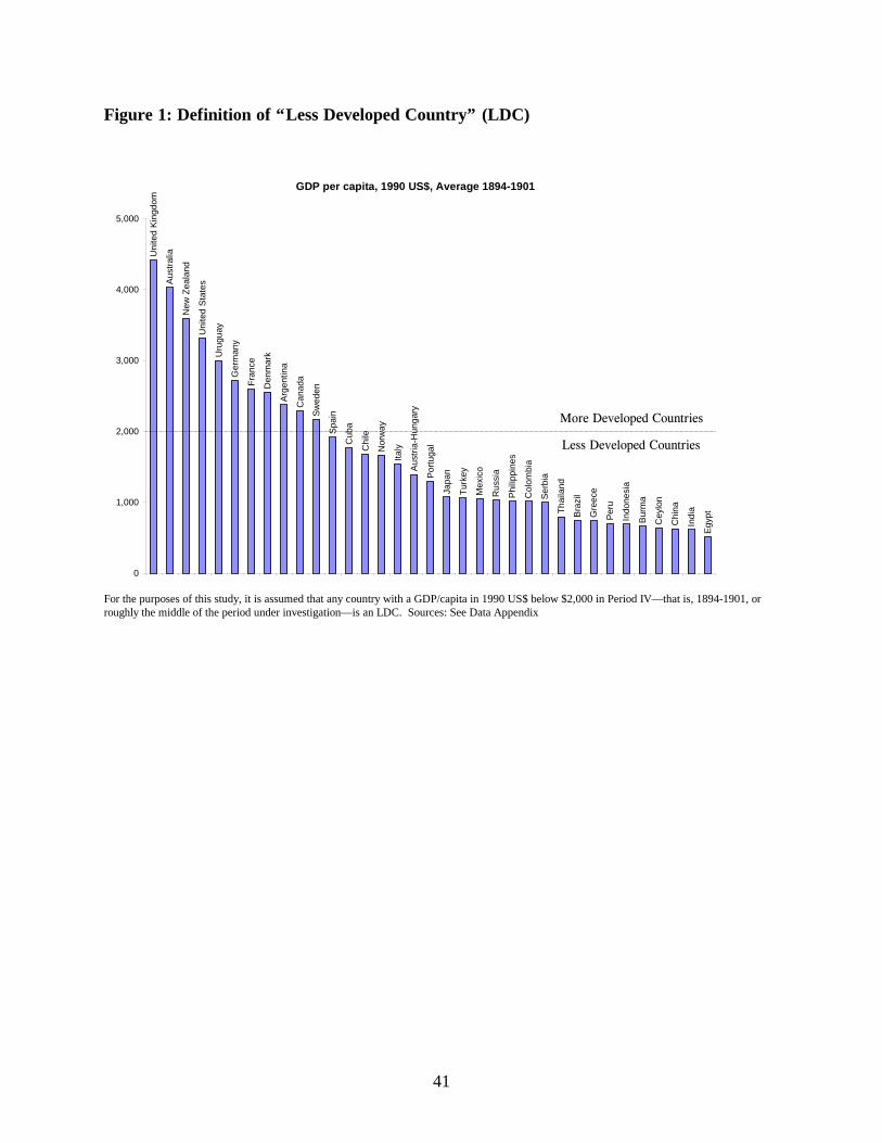
(LDC) according to GDP per capita at the turn of the century (Figure 1).

The database contains a range of variables related to market failure and capital productivity. On

the capital market failure side, it includes import duties as a fraction of total import value, colonial

affiliation, monetary regime, exchange rate variance against the pound sterling, changes in the terms of

trade, and an index combining shipping costs and distance from London. On the capital productivity

side, it includes the youth dependency ratio, net immigration rates, primary school enrollment rates,16

urbanization, and indices of natural resource abundance made popular by Sachs and Andrew Warner

(1995). The database also includes real PPP-adjusted unskilled urban wages relative to Great Britain for

thirty countries, and prices of capital equipment for eight.

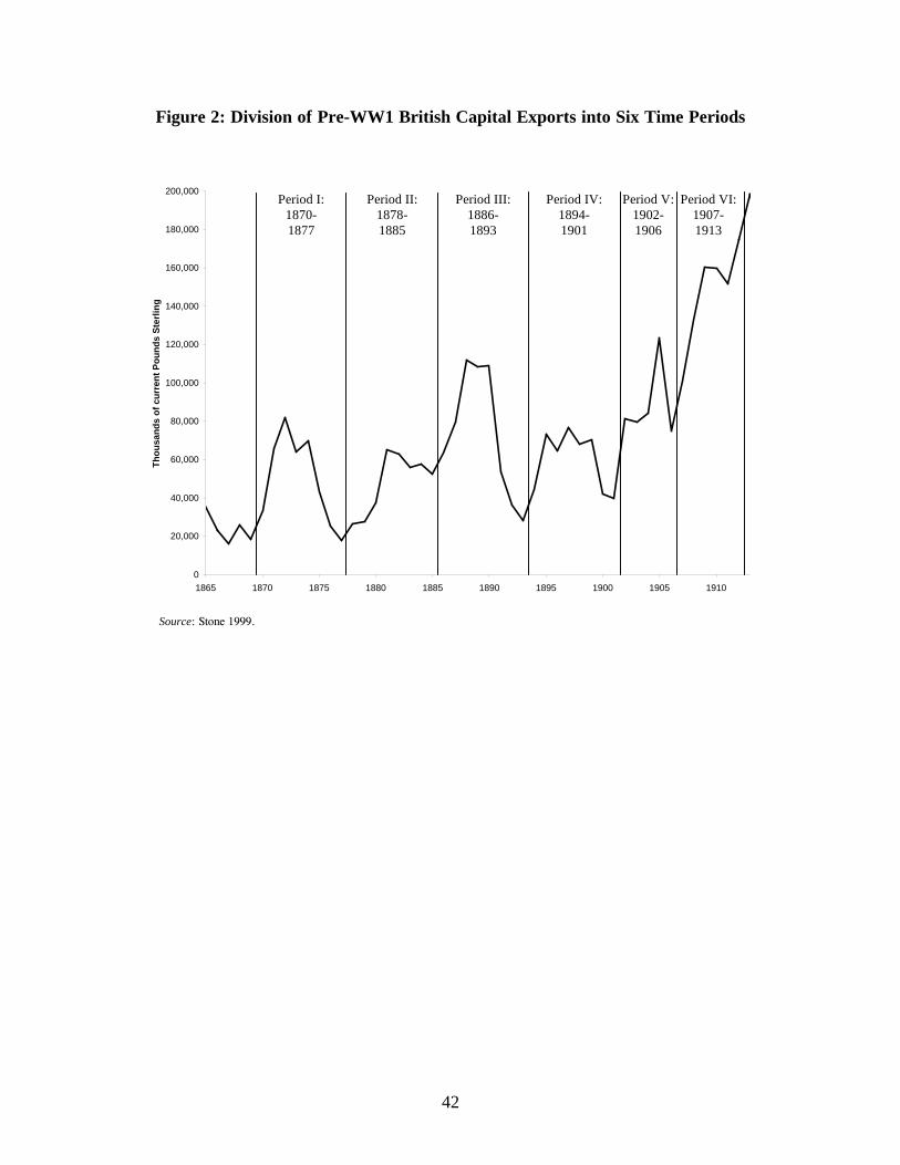
Each data point represents one country in each of six time periods, shown in Figure 2. The

decision to aggregate our annual data into multi-year periods was based on a desire to defuse the effects

of outlier years and the need for a right-hand side matrix of significant variance. Six periods were chosen

to utilize local minima as divisions between successive waves of outflows. Economists since Hobson

(1914, pp. 142-9) have divided prewar British capital exports into three periods, separated by two large

troughs. The first corresponds to a depression in the aftermath of the Franco-Prussian war and a series

15 The countries are Argentina, Australia, Austria-Hungary, Brazil, Burma, Canada, Ceylon, Chile, China,Colombia, Cuba, Denmark, Egypt, France, Germany, Greece, India, Indonesia (Dutch East Indies), Italy, Japan,Mexico, New Zealand, Norway, Peru, the Philippines, Portugal, Russia, Serbia, Spain, Sweden, Thailand (Siam),Turkey (Ottoman Empire without Egypt and European territories), the USA, and Uruguay. They are distributed:Europe 12; North America and Australasia 4; Latin America 8; Middle East 2; and Asia 8. See Data Appendix.16 Estimates of the educational attainment of the work force is unavailable for almost all of the countries in oursample, but following the suggestions of Barro and Lee (most recently, 2000), we use enrollment rates among theschool-aged fifteen years previously as a proxy for the current schooling stock per capita.

18

of defaults in 1874, and the second to economic collapse in Argentina, Australia, and elsewhere in 1890-

91. We exploit minor local minima to achieve a slightly higher resolution, balancing the need to

aggregate against our desire to reveal dynamic changes in flow determinants.17

Unlike most studies of British capital exports,18 ours focuses exclusively on what pulled British

capital into some countries versus others, rather than what pushed it out of Great Britain. Our dependent

variable is therefore the value of total British capital exported to a given country during a given period as

a fraction of all British capital exported during that period. Push effects are thus entirely eliminated.

Scale effects from market size are eliminated by the inclusion of log GDP on the right hand side.

The Determinants of Capital Destination

Our central result, presented in Tables 3, 4, and 5, is that the wealth bias was alive and well

during the latter half of the period 1870-1913, and that it can be explained in a way that is sufficient to

reject the global capital market failure view. We stress that we are not asking, as many others have,19

whether perfect global capital markets existed during this period. Instead, we are asking whether global

capital market failure can be viewed as a primary explanation for the wealth bias.

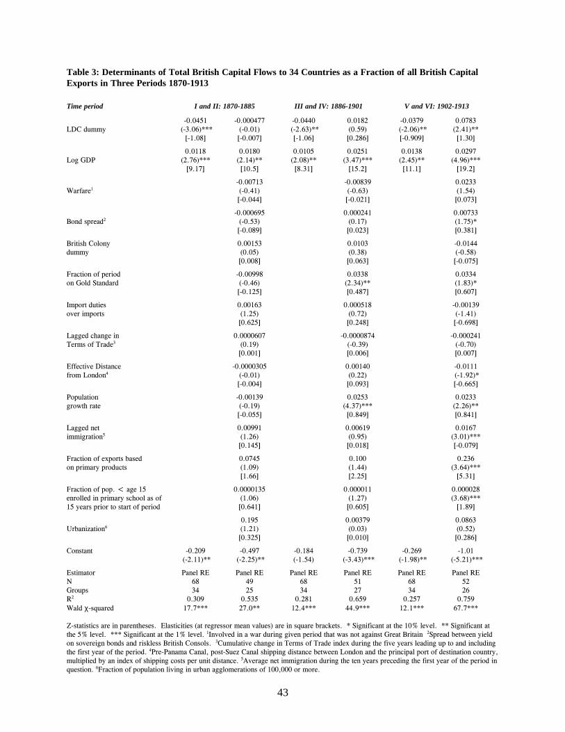
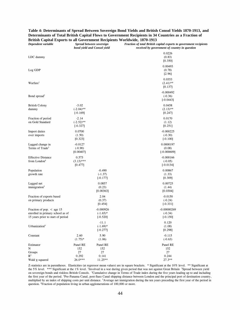
Identifying the Fundamentals That Mattered. In Table 3, note the significant, negative effect of

the LDC dummy on flows when that variable is accompanied only by log GDP. Furthermore, the

negative unit elasticity on the LDC dummy is relatively constant over time. This is one manifestation of

the wealth bias. The inclusion of proxies for global market failure and for fundamental national

characteristics eliminates this negative LDC elasticity in periods I and II, but by periods V and VI this

elasticity has become positive and statistically significant, with an elasticity of 1.3. In other words, after

17 Another concern influencing the division of flows into periods was the possible creation of a large number ofleft-hand-side zeros in a given period if the divisions were too fine, with the consequent risk of censored data andmaterial non-linearities. Given our six-period division, an average of 2.2 countries out of 34 received no Britishcapital in each period, with the largest number being 4 (in Period I) and the smallest number being 0 (in PeriodVI). The substance of our results does not depend on whether the years 1870-1913 are divided into ten, six, orthree periods, or even considered as a single pooled period; all were tested.18 Such as Richardson (1972), Cain and Hopkins (1980), Edelstein (1983), and Davis and Huttenback (1988).19 Including Bordo, Eichengreen and Kim (1998), Kohl and O’Rourke (2000), among many.

19

accounting for the effects of other variables, poor countries received more than twice the share of British

capital than did rich countries in the years leading up to World War 1. Natural resource endowment,

education, and demography dominate all other variables in terms of elasticities and statistical

significance. Capital flows are more than six times as sensitive to variation in natural resources

endowment and more than twice as sensitive to variation in education levels than they are to any

competing determinant. Minor, statistically significant determinants include participation in the Gold

Standard, effective distance from London,20 lagged net immigration, and the yield spread between

sovereign bonds and the riskless British Consol.

Rejecting the Global Capital Market Failure View of the Wealth Bias. The evidence from 1902

to 1913 is consistent with the predictions of the unproductive domestic capital view of the wealth bias,

but not with those of the global capital market failure view. The global capital market failure view

predicts that involvement in warfare should have choked off British capital inflows, that countries with a

higher sovereign bond spread should have received a smaller share of British capital, and that country

fundamentals unrelated to creditworthiness should not have affected inflows. In fact, between 1902 and

1913 involvement in warfare did not dampen capital flows, bond spreads attracted capital, and country

fundamentals were the best determinants of flows. It cannot be said that the global capital market failure

view is totally without merit; after all, the Gold Standard and effective distance from London both have

the predicted signs between 1902 and 1913. However, the failure view pales in importance compared

with the competing unproductive domestic capital view, and increasingly so as time wore on between

1870 and 1913.

How can we be sure that the �fundamentals� are not proxies for creditworthiness? Could

natural resource endowment or education have made a recipient country more creditworthy in the eyes of

British investors, rather than directly affecting the return to capital? Table 4 explores this issue. In the

20 Effective distance from London is calculated as the physical distance of the shortest available shipping routebetween London and the closest principal port of the country in question (pre-Panama Canal, post-Suez Canal)multiplied by an index of transoceanic shipping costs. See Data Appendix for details.

20

first column, the dependent variable is the spread between the yield on sovereign bonds in 27 countries

and the yield on the riskless British Consol, averaged over each of our six periods 1870-1913. The

results are consistent with the premise that the bond spread captures investment risk: British colonies and

those on the Gold Standard had lower spreads, while highly protected countries far from London had

higher spreads. In the second column, we see that natural resource endowment did not affect bond

spread in a statistically significant way, although education was a (barely) statistically significant

predictor of lower bond spread. Recall from Table 3, however, that even after accounting for the effect

of education on creditworthiness (by including bond spread as a regressor), education was one of the top

determinants of capital flows. It is for this reason that we describe natural resource endowment and

education as �fundamentals,� or factors that affect capital flows through their effect on the return to

domestic capital.

Just because the predictors of bond spread have the �right� sign does not, of course, prove

unambiguously that bond spreads capture creditworthiness. In the transition from autarky (around 1870)

to integrated world capital markets (around 1913), bond spreads would have had very different meaning:

bond spreads would have attracted capital at the start, while at the end they should have been an

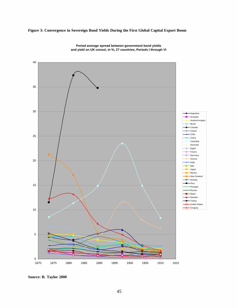
indicator of risk, thus deterring foreign capital. Figure 2 reveals a massive global convergence in bond

spreads in the years leading up to World War 1, a phenomenon discussed elsewhere (e.g. Mauro,

Sussman, and Yafeh 2000). Not only does the mean of these spreads fall from 4.07% to 1.65% between

periods III and VI, but the coefficient of variation also falls from 1.75 to 1.07. We interpret this

evidence as support for the view that bond spreads were increasingly an indicator of creditworthiness.

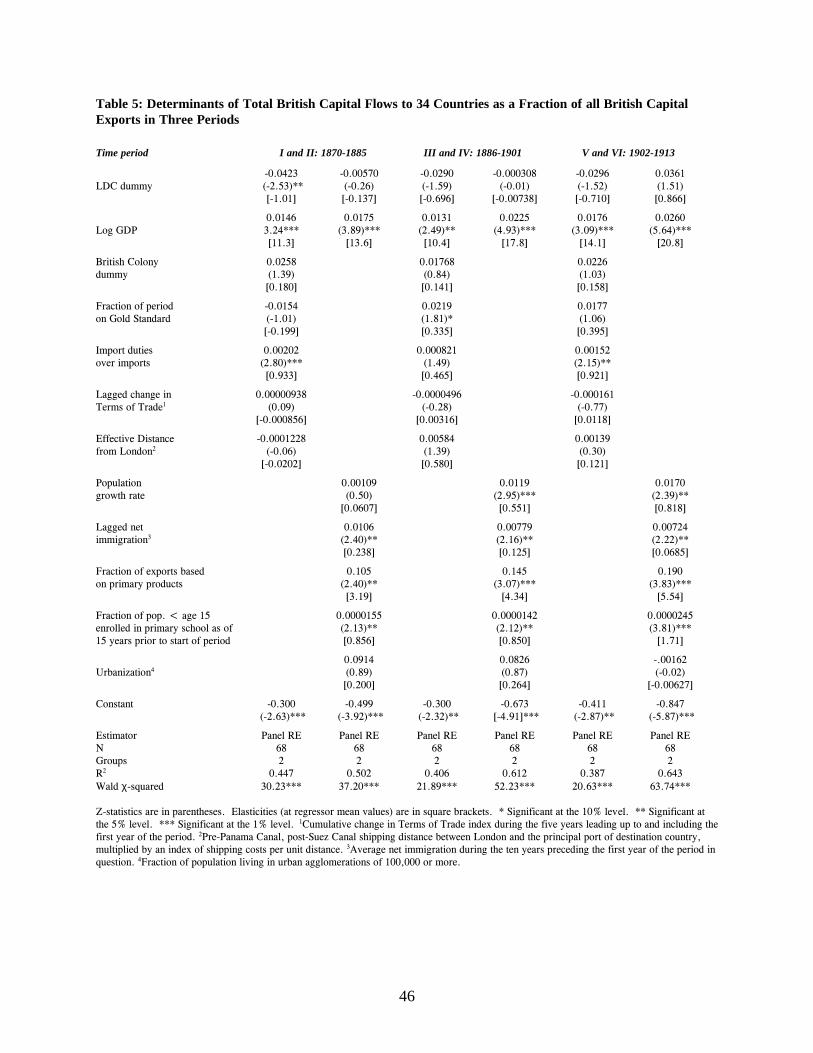
Specification. Our conclusions are robust to several changes of regression specification. One of

these, shown in Table 5, shows that the results of Table 3 do not spring in any way from a paucity in

degrees of freedom. Inclusion of just a few of the variables associated with the unproductive domestic

capital view largely reproduces the results of Table 3, while inclusion of the same number of variables

21

related to the global capital market failure view cannot explain the wealth bias.21 Why use random

effects? For example, a Hausman test on the regression in the last column of Table 3 gives a χ2(12)

statistic of 5.95, which fails to reject the null hypothesis that the random error associated with each cross

section is uncorrelated with the regressors (p-value 0.92).

Endogeneity Bias. We have treated immigration as exogenous to capital flows and to the other

fundamentals of the right-hand side. That certainly would have been so if European �push� conditions

dominated. But a rich literature makes it clear that the mass migrations were also determined by �pull�

in receiving regions (Hatton and Williamson 1998). Since we are uncertain about whether push or pull

dominated, we estimate Tables 3, 4, and 5 using lagged immigration, defined as average net immigration

during the ten years preceding the first year of the period in question.

We have also treated education and natural resource endowment as exogenous. We are

sympathetic to any argument suggesting that British investment may have raised the returns to education

in recipient countries. Note, however, that our education regressor is lagged by 15 years. We also agree

that British investment contributed to the development of natural resources in the recipient countries. But

regressing period VI capital flows on period I natural resource endowment does not alter the status of

this regressor as the primary determinant of capital flows. This is not a surprise, since less than 10% of

British capital exports were invested directly in projects to extract natural resources such as metals,

nitrates, oil, tea, coffee, and rubber (Stone 1999). The vast majority of British capital went to railroads

and other transportation infrastructure, financial institutions, factories, and communications

infrastructure�activities whose effect on the resource composition of exports is long-term rather than

immediate.

21 Neither do several other changes of specification, not reported here, alter the results of Table 3. OLS cross sectionregressions on each of the six periods reveal the same time progression in the ability of fundamentals to explainwealth bias. Division of the years 1870-1913 into ten periods rather than six gives similar results. Includingexchange rate variance or an indicator of Gold, Silver or Bimetallic standard instead of just the Gold Standard;including for variance in Terms of Trade instead of cumulative change in Terms of Trade; or defining “LDC”according to relative PPP-adjusted real wage levels do not materially alter the results.

22

Influential Observations. Although no single country received more than a quarter of British

capital in any given period, a few countries taken together received most of it. Major recipients included

the United States, Argentina, Australia, and Canada. Was one of these countries largely responsible for

the results in Table 3? Additionally, it is not known how much British investment in resource-rich

�China� was actually investment in resource-poor Hong Kong. Would the elimination of China alter the

results? The following are the elasticities of British capital share with respect to the LDC dummy from

the specification in the last column of Table 3 when various countries are omitted from the sample:

Argentina, 1.61; Australia, 1.36; Canada, 1.06; China 1.18; USA, 1.39. The elasticity on natural

resource endowment when China is omitted is 5.26. In short, none of these countries materially affect

the ability of fundamentals to explain the wealth bias between 1901 and 1913.

Global Capital Market Deepening and Transitions through Time. Table 3 documents an

upward drift in the share of British capital flows explained, and, furthermore, that the fundamentals

exhibit a stronger impact as the decades unfold.22 What made flows respond to fundamentals after the

1890s more than they had previously? Figures 2 and 3 suggest that the international capital market was

simply deeper than it had been before.23 Transoceanic trade awoke from post-Boer War depression, the

Russo-Japanese war stimulated borrowing, the Canadian and Argentine railways expanded, and British

capital spread to a wider area than ever before�including major movements to Brazil, Mexico, Chile,

Egypt, South Africa, India, Russia, and the Far East (Hobson 1914, pp. 157-8). Herbert Feis (1930, pp.

12-13) puts it thus:

Changing political relations took British capital into countries from which it had previouslyabstained--Japan [Alliance of 1902], Russia [Anglo-Russian agreement, 1907], and Turkey. Butmore important than these causes in producing a great growth in foreign investment was the factthat during the 1900-1914 period those distant lands to which the capital had been going inearlier periods, seemed to have overcome the risks and crashes of their first growth. Now in thegreater stability and greater order of their development, they needed still more capital thanbefore and offered surer return. Or—the idea presents itself in alternative form—it was as

22 This shift is statistically significant. For example, a Chow test (χ2[9]=17.96, p-value 0.0357) rejects at the 5%level the null hypothesis that the coefficients for Periods III & IV are the same as the coefficients in Periods V &VI in Table 3.23 Only about 40% of British capital exports that occurred during 1870-1914 flowed overseas before 1895.

23

though many regions of the world in which British capital had invested itself had come to fitthemselves better for the investment, learning from pioneer failures.

Robert Gallman and Lance Davis (2001, Ch. 7) provide extensive evidence of �financial deepening� in

British capital recipient countries during this period, including rising measures of total financial assets

and assets of financial intermediaries as a fraction of GNP. We suspect that regularities dictating who

got British capital prior to the 1890s are hidden by a thin global market for that capital. The deepening

of that market in the fifteen years prior to 1913 allows us to better isolate the determinants of those

flows. It is here that the evidence rejecting global-capital-market-failure explanations of the wealth bias is

strongest.

There may, of course, be other reasons why the fundamentals exhibit an increasingly powerful

influence through time. Economic historians have long argued that conventional physical capital

accumulation mattered far more in the 19th century, while human capital accumulation mattered far

more in the 20th century, the changing mode of accumulation driven by the evolution of technologies on

the demand side and/or by the release of constraints on schooling investment on the supply side. Perhaps

the increasing importance of human capital endowment as a determinant of British capital inflows simply

reflects this transition.

One explanation for the increasing importance of fundamentals over time can be easily ruled out.

If the data on British capital exports included re-investment in debt that was periodically �rolled over,�

one might expect that a country with fundamentals that attracted capital would build up a larger and

larger stock of debt over time, thus experiencing ever larger �rollover� inflows of capital. The flows

explored here do not, however, include debt rollover. Rather, they were compiled to include only �new

issues,� and only reflect actual financial transfers rather than accounting changes (Stone 1999; Jenks

1927). Furthermore, a necessary condition for this �rollover� explanation would be to observe long-term

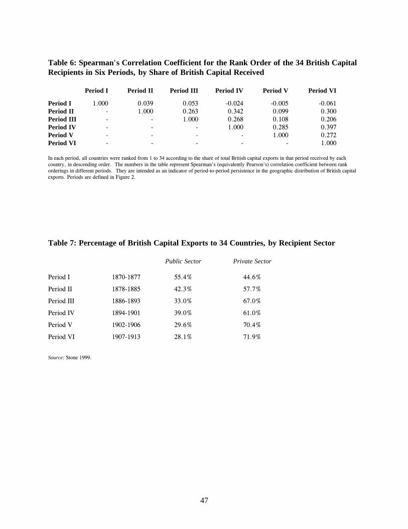
persistence in the geographical distribution of flows. Table 6 shows Spearman�s correlation coefficient

24

between the rankings of British capital recipients in the six periods; there is very little persistence in the

evidence.

Capital Flows to Governments and to the Private Sector

Disaggregating capital flows by recipient sector allows us to learn even more about how they

were determined. Table 7 shows that during most of the prewar years, British capital exports were

primarily invested in the private sector of the destination country. What drove flows to governments, and

how did these interact with flows to the private sector? The last column of Table 4 explores the

determinants of flows to governments. Abundant anecdotal evidence suggests that warfare was an

important determinant of demand for sovereign borrowing, which in itself would make capital flows to

governments unrelated to recipient country characteristics even without international market failure. There

were massive loans to the French and German governments during the Franco-Prussian War in the 1870’s,

to the South African government at the time of the Boer War in the 1890’s, and to the Japanese

government to finance its war with Russia just after 1900. For each of these countries, total wartime

sovereign borrowing dramatically exceeded the cumulative total of all peacetime borrowing during the five

decades that preceded the First World War. Contemporary observers (e.g. van Oss 1898, p. 228) likewise

identified warfare as the primary determinant of sovereign borrowing from Britain. The last column of

Table 4 confirms that warfare and British colonial status were the only determinants of borrowing by

governments that remained statistically significant throughout the capital boom. Since the analysis of

Section III showed that the global-capital-market-failure view predicts a negative coefficient on warfare,

the evidence in Table 4 rejects that view.

Yet, the last column of Table 4 does not offer very strong support for the view that “fundamentals”

determined flows to governments either. True, the lack of evidence supporting the unproductive capital

view is a necessary condition for acceptance of the capital markets failure view, not a sufficient condition.

After all, this necessary condition could easily be satisfied by the preeminence of warfare over other

considerations in sovereign borrowing behavior, and there is ample anecdotal evidence that this was indeed

25

the case. Still, historians such as Feis (1930, pp. 98-117) have documented highly unreliable contract

enforcement efforts by the British government on behalf of British investors in foreign governments that

suffered in the many defaults catalogued by Peter Lindert and Peter Morton (1989). Such interventions

were often guided more by British political or territorial aspirations than by a sense of duty to its investors.

In light of such qualitative accounts, we cannot reject global-capital-market-failure explanations for

government-bound flows, even though we have rejected such explanations for total flows.

We must be cautious, of course, in drawing a hard and clear line between flows to governments

and flows to the private sector, as Simon, Jenks and Stone defined them. For one thing, government

involvement in many of these �private sector� loans tended to be heavy�especially in the case of

railroads, the largest category of private sector borrowing. Whether through land grants, subsidies, or

loan guarantees, governments were indirect partners to many private sector investments (Nurkse 1954,

p. 749). Furthermore, when analyzing these flows from the perspective of the 21st century, we must

remember that most of these private-sector flows went to investments in what Simon (1968, p. 23) calls

�social overhead capital.� These included projects with significant positive externalities -- projects like

railroads and public utilities � projects often undertaken today by government borrowers.

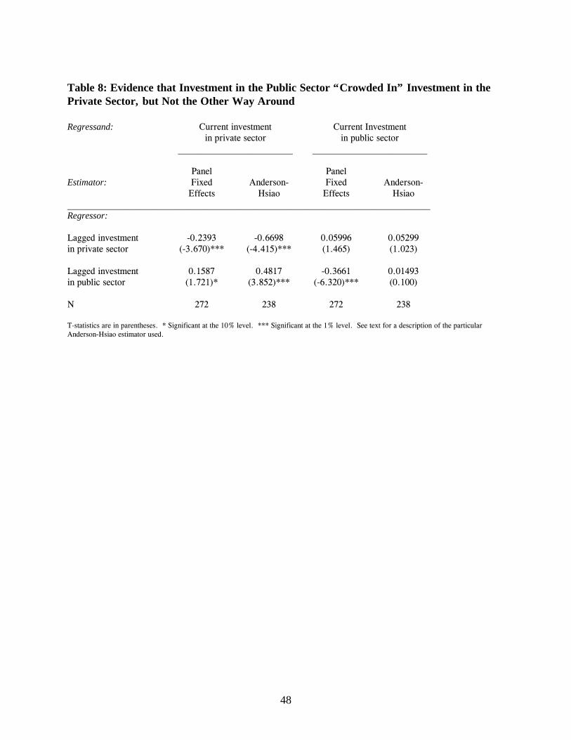
Investment in Governments Crowded-in Private Investment

Table 8 suggests that previous investment in governments �crowded in� subsequent private

sector investment. Capital flow data in this table were divided into ten periods of five years each, and

�lagged� refers to the five-year period preceding the one in question. Because two lags were necessary

for the panel fixed-effects model, the number of observations is (34 countries x 10 periods) � (34

countries x 2 lags) = 272. Similarly, the Anderson-Hsiao estimator, which uses 3 lags, lowers the

number of observations to 238.

The panel fixed-effect estimates reveal a positive effect of lagged public sector investment on

current private sector investment (significant at 9%), while the effect of lagged private sector investment

on current public sector investment is much smaller and insignificant. It is well known, however, that

26

inclusion of a lagged dependent variable in a fixed-effects panel regression can produce severely biased

coefficients, especially for small panels like this one (Nickell 1981). Anderson and Hsiao (1981) offer a

solution by instrumenting for the once-differenced dependent variable with the twice-differenced

dependent variable.24 The results of this Anderson-Hsiao estimation are also reported in Table 8. The

crowding-in effect of public sector investment on private is confirmed, and again no such causation is

seen from private sector investment to public. Note the negative coefficient for past private investment

regressed on current private investment, likely reflecting the fact that in each period private investment

was expanding into countries that had never received it before. This illustrates the again deepening of the

global capital market over time. Furthermore, it argues against geographic persistence of public (and

thus total) investment flows: public investment tended to grow in wartime and shrink in peacetime; it did

not progressively expand.

Why did crowding-in take place? One explanation might be that loaning to public entities

contributed to financial deepening: for example, investment in the government debt of South Africa

during the Boer War may have opened investors� eyes to private sector opportunities subsequently.

Alternatively, private investment followed investment in governments because governments borrowed to

make war, and the private sector subsequently borrowed to rebuild the country or to make good on

foregone private accumulation.

V. Discussion and Historiography

The question of whether pre-WWI British capital exports were driven by domestic capital

productivity or by global market failure has been around at least since C. K. Hobson, who was writing at

the capital export peak. Hobson raised the question and then offered as an explanation the declining

importance of global market failure and thus, presumably, the rising importance of capital productivity

24 Judson and Owen (1996) use a Monte Carlo approach to demonstrate that the Anderson-Hsiao estimator

27

fundamentals (Hobson 1914, p. xii). Were Hobson alive today, he probably would want to leave his

explanation unchanged. After all, the evidence we have presented suggests that the largest capital

exporter in history was indeed sending its money where it could earn the highest return, and that was

where the fundamentals served to raise capital�s productivity.

As Edelstein (1982, p. 7) points out, the idea that third factors like land could allow for

increasing returns to British capital exports in newly-settled regions goes back at least to Adam Smith

(1776, pp. 89-93). Feis (1930, pp. 25, 31) also favored third-factor fundamentals by asserting that the

�British investor was sending his capital where there was the growth of youth, and where the land was

yielding riches to the initial application of human labor and technical skill,� undeterred by �[s]trong

risks, bad climates� and �isolation.� After clearly identifying the wealth bias by stating that �income per

head in the principal debtor countries of the nineteenth century�the newly settled regions�can never

have been far below European levels,� Ragnar Nurkse (1954, p. 757) also concludes that capital was

attracted �not to the neediest countries with their �teeming millions,�� but rather chased the �great

migration� to the �spacious, fertile, and virtually empty plains� of certain countries (pp. 745, 750).

Thus, our answer to Hobson�s question is not new.

Second-Order Determinants of Flows

The contribution of this paper is to provide empirical confirmation of the views of pioneer

analysts of the global capital market and to show that they are superior to competitors. We now consider

several popular competing explanations of British capital flows which we find to be of only secondary

importance.

Terms of Trade. We can find no evidence supporting the view that capital flows were primarily

driven by recent terms of trade shocks. Brinley Thomas (1968, pp. 49-50) felt that �movements in the

terms of trade are to be looked upon more as consequences than as causal forces� of capital flows.

essentially eliminates this bias, though it is not as efficient as other methods for small panels.

28

�Cairncross [1953],� he writes, �has to go out of his way to find reasons why heavy British capital

exports in the eighties should have coincided with a deterioration in the terms of trade of the borrowing

countries, for the link seemed to work so well in the nineties and the 1900s.� In defense of his critique,

Thomas expounds a plausible model of causation from capital flows to terms of trade. Our results

support his critique (but not necessarily his model).

Colonial Status. Many historians have viewed British capital exports as part and parcel of

British colonial expansion. This view appears reasonable in light of such developments as the 1900

revision of the Colonial Stocks Act, which promoted Empire investment by allowing registered securities

in British colonies and dominions to be purchased by trust bodies and large institutional investors

previously banned from foreign investment (Feis 1930, pp. 92-95). Yet, many have criticized this view

by simply citing counter-examples like non-Empire capital flows to Argentina and the United States (e.g.

Simon 1968, p. 24; Platt 1986, p. 25). What we add here is multivariate, quantitative support their

univariate, qualitative analysis. Our results leave no doubt whatsoever that markets mattered far more

than flag for private-sector British investment heading abroad. British colonies did get a larger share of

capital flows to government recipients, but market concern was the first-order determinant of destination.

The Gold Standard. Eichengreen (1996, p. 18) has stated unequivocally that in the 1870s,

�[i]ndustrialization rendered the one country already on gold, Great Britain, the world�s leading

economic power and the main source of foreign finance. This encouraged other countries seeking to

trade with and import capital from Britain to follow its example.�25 While we also detect a positive and

statistically significant effect of participation in the Gold Standard, in Period III and after (as more and

more countries joined the club), the elasticity of this effect on investment flows is much lower than the

effects of natural resources, education, demographic structure, and capital scarcity.

There are many possible explanations for our finding, but the prominent one is that the effects of

economic, demographic and geographic fundamentals simply outweighed the effects of the Gold Standard.

25 For an anecdote on how capital flows to Brazil stagnated after departure from the Gold Standard, see

29

Michael Bordo and Anna Schwartz (1996, p. 41) find anecdotal evidence that “adherence to the rule by

Argentina may have had some marginal influence on capital calls … before 1890 ... but that the key

determinant was the opening up of the country’s vast resources to economic development once unification

and a modicum of political stability were achieved.” We confirm the Bordo and Schwartz Argentina

finding on a global scale: if the fundamentals were not satisfied, going on gold didn’t bring in the capital.

Based on a sample of nine capital-importing countries, Bordo and Hugh Rockoff (1996) argue that

adopting the Gold Standard lowered the costs of borrowing in world capital markets, and that it served as a

“good housekeeping seal of approval.” However, Bordo and Rockoff do not control for any economic,

demographic or geographic fundamentals. Their view is also inconsistent with the more recent empirical

work of Christopher Meissner (2000, p. 22) who, with a larger sample of 19 countries, rejects the idea that

going on gold mattered after controlling for fundamentals.

VI. Conclusion

During the first globalization boom prior to World War I, British capital did not go to poor,

labor abundant economies. We call this the wealth bias. The evidence rejects the global-capital-market-

failure explanation of the wealth bias. British foreign investment went where it was most profitable�

chasing natural resources, educated populations, migrants, and young populations. Flows to private

sector investment opportunities abroad were also encouraged by previous investments in government-

financed projects.

We should stress what our results do not imply. They do not suggest that global capital market

failure was absent in the years leading up to the First World War. Rather, they suggest that the observed

wealth bias was not explained by global capital market failure. It is surely possible to imagine capital

flows that -- although unobservable because global capital market failure stopped them cold -- would

have gone primarily to capital-poor countries. One candidate for such flows is investment in

Eichengreen (1992, p. 60).

30

manufacturing, which accounted for less than four percent of British capital exports (Simon 1968, p. 23).

Edelstein (1982, pp. 41-2) points to market failure as the cause of this tiny figure, citing insuperable

informational advantages of local manufacturers in local input and output markets. He also mentions the

increasing importance of tariff barriers abroad in keeping British manufacturing investment at home.

Feis (1930, p.31) agrees, calling foreign industrial investment �risky [and] difficult to manage well from

a distance.� We do not have the evidence to assert that such imaginary flows would also have chased

resources, education, migrants and youth.

British capital flowing to sub-saharan Africa was modest, but we certainly do not claim that this

region lacked natural resources. Perhaps there is an extremely low GDP per capita threshold below

which capital market failure is the primary determinant of capital flows. Since this level lies below the

lowest GDP per capita in our data, however, we cannot test this hypothesis. We can only reiterate that

the data cover about nine tenths of the world population and almost all of the global economy of that

time, as well as an extremely wide range of GDP per capita levels from the very wealthy to the very

poor.

Global capital market failure did not determine how large a slice of the British-capital-export pie

was received by a given capital-importing country at the height of the boom. Whether the relative size of

that slice would have changed had the entire pie been augmented by a total absence of any global capital

market failure is an entirely different question that may never be answered. We have also shown that the

major fundamentals that determined where capital went were, in order of importance, natural resource

endowment, schooling, and demographic attributes. Whether the fundamentals driving capital exports in

the late 19th century were the same as those driving capital exports in the late 20th century is another

question that can be answered, but must await future research.

31

References

Abramovitz, M., 1968, �The Passing of the Kuznets Cycle,� Economica 35: 349-67.

Anderson, T. W. and C. Hsiao, 1981, �Estimation of Dynamic Models with Error Components,�

Journal of the American Statistical Association, 76 (September): 598-606.

Banerjee, A. V., 1992, �A Simple Model of Herd Behavior,� Quarterly Journal of Economics, 107 (3):

797-818.

Barro, R. J., 1989, �Economic Growth in a Cross-Section of Countries,� NBER Working Paper 3120,

National Bureau of Economic Research, Cambridge, Mass.

Barro, R. J. and J-W. Lee, 2000, �International Data on Educational Attainment: Updates and

Implications,� NBER Working Paper 7911, National Bureau of Economic Research, Cambridge,

Mass. (September).

Barro, R. J. and X. Sala-I-Matin, 1995, Economic Growth (New York: McGraw-Hill).

Bloom, D. and J. Sachs, 1998, �Geography, Demography, and Economic Growth in Africa,” Brookings

Papers on Economic Activity, 2 (Washington, D.C.: Brookings Institution): 207-95.

Bloom, D. and J. G. Williamson, 1998, �Demographic Transitions and Economic Miracles in Emerging

Asia,� World Bank Economic Review 12 (3): 419-55.

Bohn, H. and L. L. Tesar, 1996, �US Equity Investment in Foreign Markets: Portfolio Rebalancing or

Return Chasing?� American Economic Review 86 (May): 77-81.

Bordo, M. D., B. Eichengreen, and J. Kim, 1998, �Was There Really an Earlier Period of International

Financial Integration Comparable to Today?� NBER Working Paper 6738, National Bureau of

Economic Research, Cambridge, Massachusetts.

Bordo, M. D. and F. E. Kydland, 1995, �The Gold Standard as a Rule: An Essay in Exploration,�

Explorations in Economic History 32 (October): 423-64.

32

Bordo, M. D. and H. Rockoff, 1996, �The Gold Standard as a �Good Housekeeping Seal of Approval�,�

Journal of Economic History 56 (2): 389-428.

Bordo, M. D. and A. J. Schwartz, 1996, "The Operation of the Specie Standard: Evidence for Core and

Peripheral Countries 1880-1990," in J. Braga de Macedo, B. Eichengreen and J. Reis, eds.,

Currency Convertibility: The Gold Standard and Beyond (New York: Routledge).

Boyd, J. H. and B. D. Smith, 1992, �Intermediation and the Equilibrium Allocation of Investment

Capital,� Journal of Monetary Economics 30: 409-32.

Cain, P. J. and A. G. Hopkins, 1980, �The Political Economy of British Expansion Overseas, 1750-

1914,� Economic History Review, Second Series, 4 (November): 463-90.

Cairncross, A., 1953, Home and Foreign Investment (Cambridge: Cambridge University Press).

Clark, G., 1987, �Why Isn�t the Whole World Developed? Lessons from the Cotton Mills,” Journal of

Economic History 47 (1): 141-73.

Clemens, M. A., ongoing, �Where Has US Foreign Capital Gone? The Lucas Paradox in the Late 20th

Century.�

Collins, W. J. and J. G. Williamson, 2001, �Capital Goods Prices and Investment, 1870-1950,” Journal

of Economic History 61 (March): 59-94.

Cont, R., and J.-P. Bouchaud, 2000, �Herd Behavior and Aggregate Fluctuations in Financial Markets,�

Macroeconomic Dynamics 4 (June):170-96.

Cox, J. C., J. E. Ingersoll Jr., and S. A. Ross, 1985, �An Intertemporal General Equilibrium Model of

Asset Prices,� Econometrica 53 (March): 363-84.

Davis, L. E. and R. A. Huttenback, 1988, Mammon and the Pursuit of Empire: The Economics of

British Imperialism (New York: Cambridge University Press).

DeLong, J. B. and L. Summers, 1991, �Equipment Investment and Economic Growth,� Quarterly

Journal of Economics 106: 445-502.

33

DiTella, G., 1982, �The Economics of the Frontier,� in C. P. Kindleberger and G. DiTella (eds.),

Economics in the Long View, Vol. 1 (New York: New York University Press).

Eatwell, J., M. Milgate, and P. Newman, eds., 1987, The New Palgrave: A Dictionary of Economics

(New York: W. W. Norton).

Edelstein, M., 1976, �Realized Rates of Return on UK Home and Overseas Portfolio Investment in the

Age of High Imperialism,� Explorations in Economic History 13: 283-329.

Edelstein, M., 1981, �Foreign Investment and Empire 1860-1914,� in The Economic History of Britain

Since 1700, Vol. 2, eds. R. Floud and D. N. McCloskey (Cambridge: Cambridge University

Press).

Edelstein, M., 1982, Overseas Investment in the Age of High Imperialism (New York: Columbia

University Press).

Edelstein, M., 1983, �Foreign Investment and Empire 1860-1914,� in R. Floud and D. McCloskey,

eds., The Economic History of Britain since 1700, Vol. 2: 1860 to the 1970s (New York:

Cambridge University Press).

Eichengreen, B., 1992, Golden Fetters: The Gold Standard and the Great Depression 1919-1939

(Oxford: Oxford University Press).

Eichengreen, B., 1996, Globalizing Capital: A History of the International Monetary System (Princeton,

New Jersey: Princeton University Press).

Faini, R., 1996, �Increasing Returns, Migrations, and Convergence,� Journal of Development

Economics 49:121-36.

Feis, H., 1930, Europe, The World’s Banker 1870-1914 (New Haven, Conn.: Yale University Press).

Gallman, R. E. and L. E. Davis, 2001, Evolving Financial Markets and International Capital Flows:

Britain, the Americas, and Australia, 1865-1914 (New York: Cambridge University Press).

Gertler, M. and K. Rogoff, 1990, �North-South Lending and Endogenous Domestic Capital Market

Inefficiences,� Journal of Monetary Economics 26: 246-66.

34

Glaeser, E. L., D. I. Laibson, J. A. Scheinkman, and C. L. Soutter, 2000, �Measuring Trust,�

Quarterly Journal of Economics, 115 (3):811-46.

Gordon, R. H. and A. L. Bovenberg, 1996, �Why Is Capital So Immobile Internationally? Possible

Explanations and Implications for Capital Income Taxation,� American Economic Review, 86

(5):1057-75.

Green, A., and M. C. Urquhart, 1976, �Factor and Commodity Flows in the International Economy of

1870-1914: A Multi-Country View,� Journal of Economic History 36: 217-52.

Hanson, J. R., II, 1999, �Culture Shock and Direct Investment in Poor Countries,� Journal of Economic

History 59 (1): 1-16.

Hatton, T. J. and J. G. Williamson, 1998, The Age of Mass Migration (Oxford: Oxford University

Press).

Higgins, M. D., 1993, �Why Capital Doesn�t Flow from Rich to Poor Countries,� mimeo., Department

of Economics, Harvard University.

Higgins, M. D., and J. G. Williamson, 1997, "Age Structure Dynamics in Asia and Dependence on

Foreign Capital," Population and Development Review 23 (2): 261-93.

Hobson, C. K., 1914, The Export of Capital (London: Constable).

Hymer, S. H., 1976, The International Operations of National Firms: A Study of Direct Foreign

Investment (Cambridge, Mass.: MIT Press).

Jenks, L. H., 1927, The Migration of British Capital to 1875 (New York: Alfred A. Knopf).

Jones, C. I., 1994, �Economic Growth and the Relative Price of Capital,� Journal of Monetary

Economics 34: 359-82.

Judson, R. A. and A. L. Owen, 1996, �Estimating Dynamic Panel Data Models: A Practical Guide for

Macroeconomists,� Federal Reserve Board of Governors, Washington, D.C., mimeo.

35

King, R. G. and S. T. Rebelo, 1989, �Transitional Dynamics and Economic Growth in the Neoclassical

Model,� NBER Working Paper 3185, National Bureau of Economic Research, Cambridge,

Mass.

Kohl, R. and K. H. O�Rourke, 2000, �What�s New about Globalisation: Implications for Income

Inequality in Developing Countries,� Poverty and Income Inequality in Developing Countries

Discussion Paper Series, OECD, Paris.

Kuznets, S., 1958, "Long Swings in the Growth of Population and in Related Economic Variables,"

Proceedings of the American Philosophical Society 102 (1): 25-52.

Lane, P. and G. M. Milesi-Ferretti, 1999, �The External Wealth of Nations: Measures of Foreign

Assets and Liabilities for Industrial and Developing Countries,� CEPR Discussion Paper 2231,

Centre for Economic Policy Research, London.

Lindert, P. H. and P. J. Morton, 1989, �How Sovereign Debt Has Worked,� in J. D. Sachs, ed.,

Developing Country Debt and the World Economy (Chicago: The University of Chicago Press).

List, F., 1856, The National System of Political Economy (Fairfield, New Jersey: Augustus M. Kelley

Publishers, reprinted 1991).

Lucas, R., 1990, �Why Doesn�t Capital Flow from Rich to Poor Countries?� American Economic

Review 80 (May): 92-6.

Mauro, P., N. Sussman and Y. Yafeh, 2000, �Emerging Market Bond Spreads: Then Versus Now,�

IMF Working Paper 00/190, International Monetary Fund, Washington, DC.

Meissner, C. M., 2000, �A New World Order: Explaining the Emergence of the Classical Gold

Standard,� mimeo. Department of Economics, University of California at Berkeley (November).

Neal, L., 1990, The Rise of Financial Capitalism: International Capital Markets in the Age of Reason,

(New York: Cambridge University Press).

Nickell, S., 1981, �Biases in Dynamic Models with Fixed Effects,� Econometrica 49 (November):

1417-26.

36

Nurkse, R., 1954, "International Investment To-Day in the Light of Nineteenth-Century Experience,"

Economic Journal 64 (December): 744-58.

Obstfeld, M., and A. M. Taylor, 1998, "The Great Depression as a Watershed: International Capital

Mobility in the Long Run," in M. D. Bordo, C. D. Goldin and E. N. White (eds.), The Defining

Moment: The Great Depression and the American Economy in the Twentieth Century (Chicago:

University of Chicago Press): 353-402.

Obstfeld, M. and A. M. Taylor, 2001, �Globalization and Capital Markets,� presented at the National

Bureau of Economic Research Conference Globalization in Historical Perspective, Santa

Barbara, California May 4-5, 2001.

O�Rourke, K. H., 1992, �Why Ireland Emigrated: A Positive Theory of Factor Flows,� Oxford

Economic Papers 44: 322-40.

O'Rourke, K. H., 2000, �Tariffs and Growth in the Late 19th Century,� Economic Journal 110 (April):

456-83.

O�Rourke, K. H., and J. G. Williamson, 1999, Globalization and History (Cambridge, Mass.: MIT

Press).

Pigou, A. C., 1906, Protective and Preferential Import Duties (London: Frank Cass, reprinted 1968).

Platt, D. C. M., 1986, Britain’s Overseas Investment on the Eve of the First World War: The Use and

Abuse of Numbers (London: MacMillan).

Polyani, K., 1944, The Great Transformation: The Political and Economic Origins of Our Time (New

York: Rinehart).

Putnam, R., 1995, �Bowling Alone: America�s Declining Social Capital,� Journal of Democracy 6

(January): 65-78.

Razin, A., E. Sadka and C-W. Yuen, 1999, �Excessive FDI Flows under Asymmetric Information,�

Working Paper No. 27-99, The Eitan Berglas School of Economics, Tel Aviv University, Tel

Aviv, Israel.

37

Reisen, H., 1994, �Public Finance in Developing Countries and the Attraction of Foreign Capital,� in

Debt, Deficits and Exchange Rates: Essays on Financial Interdependence and Development

(Paris: Organization for Economic Cooperation and Development).

Richardson, H. W., 1972, �British Emigration and Overseas Investment,� Economic History Review,

Second Series, 25 (February): 99-113.

Sachs, J. D. and A. M. Warner, 1995, �Natural Resource Abundance and Economic Growth,� NBER

Working Paper 5398, National Bureau of Economic Research, Cambridge, Mass.

Simon, M., 1968, �The Pattern of New British Portfolio Foreign Investment, 1865-1914,� in A. R.

Hall, ed., The Export of Capital from Britain 1870-1914 (London: Methuen).

Smith, A., 1776, An Inquiry into the Nature and Causes of the Wealth of Nations (New York: The

Modern Library, reprinted 1937).

Stone, I., 1999, The Global Export of Capital from Great Britain, 1865-1914 (New York: St. Martin�s

Press).

Stone, I., 2000, personal communication.

Taylor, A. M., 1998, �On the Costs of Inward-Looking Development: Historical Perspectives on Price

Distortions, Growth, and Divergence in Latin America from the 1930s to the 1980s,� Journal of

Economic History 58 (1): 1-28.

Taylor, A. M., and J. G. Williamson, 1994, �Capital Flows to the New World as an Intergenerational

Transfer,� Journal of Political Economy 102 (April): 348-71.

Taylor, B., 2000, Encyclopedia of Global Financial Markets (Los Angeles: Global Financial Data).

Thomas, B., 1954, Migration and Economic Growth (Cambridge: Cambridge University Press).

Tobin, J., 1996, �On the Internationalization of Portfolios,� in Essays in Economics: National and

International (Cambridge, Mass.: MIT Press).

Tornell, A. and A. Velasco, 1992, �The Tragedy of the Commons and Economic Growth: Why Does

Capital Flow from Poor to Rich Countries?� Journal of Political Economy 100 (6): 1208-31.

38

Tortella, G., 1994, �Patterns of Economic Retardation and Recovery in South-Western Europe in the

Nineteenth and Twentieth Centuries,� Economic History Review 47 (1): 1-21.

van Oss, S. F. ed, 1898, Introduction to Fenn on the Funds, 16th ed., London., p. ix, reprinted in W.

H. B. Court, 1965, British Economic History 1870-1914: Commentary and Documents

(Cambridge: Cambridge University Press).

Vernon, R., 1966, �International Investment and International Trade in the Product Cycle,� Quarterly

Journal of Economics 80 (May): 190-207.

Williamson, J. G., 1964, American Growth and the Balance of Payments, 1820-1913 (Chapel Hill,

North Carolina: University of North Carolina Press).

39

Table 1: Distribution of European Foreign Investment 1913-1914 (in percent)

_____________________________________________________________________________

Destination Britain France Germany_____________________________________________________________________________

Eastern Europe 3.6 35.5 27.7Western Europe 1.7 14.9 12.7Europe (not specified) 0.5 3.3 5.1Total Europe 5.8 53.8 45.5

Latin America 20.1 13.3 16.2North America and Australasia 44.8 4.4 15.7Other New World (not specified) 2.8 0.0 2.1Total New World 67.7 17.7 34.0

Asia and Africa 26.5 28.4 20.5

Total 100.0 100.0 100.0_____________________________________________________________________________

Sources and Notes: O�Rourke and Williamson (1999, p. 229), taken from Feis (1930). Columns may not add up due to rounding. Turkey isallocated to Asia.

40

Table 2: Wealth Bias During the Two Great Capital Export Booms

Time period 1907-1913 1992-1998

Annual average gross Annual average change in stockDependent variable British capital received of private capital liabilities

(flow, in 1990 US$) (flow, in 1990 US$)

0.000208 0.00467GDP, 1990 US$ (3.32)*** (8.68)***

[0.534] [0.624]

10,700 97,900GDP per capita, 1990 US$ (2.43)** (2.20)**

[0.965] [0.410]

Constant -11,100,000 -44,700,000(-1.06) (-0.11)

Estimator OLS OLSN 34 155R2 0.414 0.463

t-statistics are in parentheses. Elasticities (at average regressor values) are in square brackets. *** Significant atthe 1% level. ** Significant at the 5% level. Source for 1992-1998 data: Capital flows from InternationalMonetary Fund 2000 International Financial Statistics CD-ROM, rest from World Bank 2000 World DevelopmentIndicators CD-ROM.

41

Figure 1: Definition of “Less Developed Country” (LDC)

For the purposes of this study, it is assumed that any country with a GDP/capita in 1990 US$ below $2,000 in Period IV—that is, 1894-1901, orroughly the middle of the period under investigation—is an LDC. Sources: See Data Appendix

GDP per capita, 1990 US$, Average 1894-1901

Uni

ted

King

dom

Aust

ralia

New

Zea

land

Uni

ted

Stat

es

Uru

guay

Ger

man

y

Fran

ce

Den

mar

k

Arge

ntin

a

Can

ada

Swed

en

Spai

n

Cub

a

Chi

le

Nor

way

Italy

Aust

ria-H

unga

ry

Portu

gal

Japa

n

Turk

ey

Mex

ico

Rus

sia

Phili

ppin

es

Col

ombi

a

Serb

ia

Thai

land

Braz

il

Gre

ece

Peru

Indo

nesi

a

Burm

a

Cey

lon

Chi

na

Indi

a

Egyp

t

0

1,000

2,000

3,000

4,000

5,000

More Developed Countries

Less Developed Countries

42

Figure 2: Division of Pre-WW1 British Capital Exports into Six Time Periods

Source: Stone 1999.

Period I:1870-1877

Period II:1878-1885

Period III:1886-1893

Period IV:1894-1901

Period V:1902-1906

Period VI:1907-1913

0

20,000

40,000

60,000

80,000

100,000

120,000

140,000

160,000

180,000

200,000

1865 1870 1875 1880 1885 1890 1895 1900 1905 1910

Thou

sand

s of

cur

rent

Pou

nds

Ster

ling

43

Table 3: Determinants of Total British Capital Flows to 34 Countries as a Fraction of all British CapitalExports in Three Periods 1870-1913

Time period I and II: 1870-1885 III and IV: 1886-1901 V and VI: 1902-1913

-0.0451 -0.000477 -0.0440 0.0182 -0.0379 0.0783LDC dummy (-3.06)*** (-0.01) (-2.63)** (0.59) (-2.06)** (2.41)**

[-1.08] [-0.007] [-1.06] [0.286] [-0.909] [1.30]

0.0118 0.0180 0.0105 0.0251 0.0138 0.0297Log GDP (2.76)*** (2.14)** (2.08)** (3.47)*** (2.45)** (4.96)***

[9.17] [10.5] [8.31] [15.2] [11.1] [19.2]

-0.00713 -0.00839 0.0233Warfare1 (-0.41) (-0.63) (1.54)

[-0.044] [-0.021] [0.073]

-0.000695 0.000241 0.00733Bond spread2 (-0.53) (0.17) (1.75)*

[-0.089] [0.023] [0.381]

British Colony 0.00153 0.0103 -0.0144dummy (0.05) (0.38) (-0.58)

[0.008] [0.063] [-0.075]

Fraction of period -0.00998 0.0338 0.0334on Gold Standard (-0.46) (2.34)** (1.83)*

[-0.125] [0.487] [0.607]

Import duties 0.00163 0.000518 -0.00139over imports (1.25) (0.72) (-1.41)

[0.625] [0.248] [-0.698]

Lagged change in 0.0000607 -0.0000874 -0.000241Terms of Trade3 (0.19) (-0.39) (-0.70)

[0.001] [0.006] [0.007]

Effective Distance -0.0000305 0.00140 -0.0111from London4 (-0.01) (0.22) (-1.92)*

[-0.004] [0.093] [-0.665]

Population -0.00139 0.0253 0.0233growth rate (-0.19) (4.37)*** (2.26)**

[-0.055] [0.849] [0.841]

Lagged net 0.00991 0.00619 0.0167immigration5 (1.26) (0.95) (3.01)***

[0.145] [0.018] [-0.079]

Fraction of exports based 0.0745 0.100 0.236on primary products (1.09) (1.44) (3.64)***

[1.66] [2.25] [5.31]

Fraction of pop. < age 15 0.0000135 0.000011 0.000028enrolled in primary school as of (1.06) (1.27) (3.68)***15 years prior to start of period [0.641] [0.605] [1.89]

0.195 0.00379 0.0863Urbanization6 (1.21) (0.03) (0.52)

[0.325] [0.010] [0.286]

Constant -0.209 -0.497 -0.184 -0.739 -0.269 -1.01 (-2.11)** (-2.25)** (-1.54) (-3.43)*** (-1.98)** (-5.21)***

Estimator Panel RE Panel RE Panel RE Panel RE Panel RE Panel REN 68 49 68 51 68 52Groups 34 25 34 27 34 26R2 0.309 0.535 0.281 0.659 0.257 0.759Wald χ-squared 17.7*** 27.0** 12.4*** 44.9*** 12.1*** 67.7***

Z-statistics are in parentheses. Elasticities (at regressor mean values) are in square brackets. * Significant at the 10% level. ** Significant atthe 5% level. *** Significant at the 1% level. 1Involved in a war during given period that was not against Great Britain 2Spread between yieldon sovereign bonds and riskless British Consols. 3Cumulative change in Terms of Trade index during the five years leading up to and includingthe first year of the period. 4Pre-Panama Canal, post-Suez Canal shipping distance between London and the principal port of destination country,multiplied by an index of shipping costs per unit distance. 5Average net immigration during the ten years preceding the first year of the period inquestion. 6Fraction of population living in urban agglomerations of 100,000 or more.

44

Table 4: Determinants of Spread Between Sovereign Bond Yields and British Consol Yields 1870-1913, andDeterminants of Total British Capital Flows to Government Recipients in 34 Countries as a Fraction ofBritish Capital Exports to all Government Recipients Worldwide, 1870-1913Dependent variable Spread between sovereign Fraction of total British capital exports to government recipients

bond yield and Consol yield received by government of country in question

0.0226LDC dummy (0.83)

[0.350]

0.00493Log GDP (0.78)

[2.96]

0.0353Warfare1 (2.41)**

[0.137]

-0.000492Bond spread2 (-0.36)

[-0.0443]

British Colony -3.02 0.0458dummy (-2.04)** (2.13)**

[-0.169] [0.247]

Fraction of period -2.14 0.0170on Gold Standard (-2.52)** (1.12)

[-0.327] [0.251]

Import duties 0.0700 -0.000225over imports (1.50) (-0.30)

[0.323] [-0.100]

Lagged change in -0.0127 0.0000197Terms of Trade3 (-0.90) (0.08)

[0.00407] [-0.000609]

Effective Distance 0.573 -0.000166from London4 (3.13)*** (-0.05)

[0.477] [-0.0134]

Population -0.490 0.00867growth rate (-1.37) (1.33)

[-0.177] [0.309]

Lagged net 0.0857 0.00725immigration5 (0.23) (1.44)

[0.00363] [0.0304]

Fraction of exports based 2.04 -0.0150on primary products (0.37) (-0.24)

[0.454] [-0.331]

Fraction of pop. < age 15 -0.000926 -0.00000269enrolled in primary school as of (-1.65)* (-0.34)15 years prior to start of period [-0.520] [-0.150]

-11.1 0.120Urbanization6 (-1.69)* (1.08)

[-0.277] [0.298]

Constant 2.60 5.90 -0.115(1.75)* (1.06) (-0.63)

Estimator Panel RE Panel RE Panel REN 152 152 152Groups 27 27 27R2 0.292 0.141 0.244Wald χ-squared 26.0*** 11.25** 27.3**

Z-statistics are in parentheses. Elasticities (at regressor mean values) are in square brackets. * Significant at the 10% level. ** Significant atthe 5% level. *** Significant at the 1% level. 1Involved in a war during given period that was not against Great Britain 2Spread between yieldon sovereign bonds and riskless British Consols. 3Cumulative change in Terms of Trade index during the five years leading up to and includingthe first year of the period. 4Pre-Panama Canal, post-Suez Canal shipping distance between London and the principal port of destination country,multiplied by an index of shipping costs per unit distance. 5Average net immigration during the ten years preceding the first year of the period inquestion. 6Fraction of population living in urban agglomerations of 100,000 or more.

45

Figure 3: Convergence in Sovereign Bond Yields During the First Global Capital Export Boom

Source: B. Taylor 2000

Period average spread between government bond yieldsand yield on UK consol, in %, 27 countries, Periods I through VI

0

5

10

15

20

25

30

35

40

1870 1875 1880 1885 1890 1895 1900 1905 1910 1915

ArgentinaAustraliaAustria-HungaryBrazilCanadaCeylonChileChinaColombiaDenmarkEgyptFranceGermanyGreeceIndiaItalyJapanMexicoNew ZealandNorwayPeruPortugalRussiaSpainSwedenTurkeyUnited StatesUruguay

46

Table 5: Determinants of Total British Capital Flows to 34 Countries as a Fraction of all British CapitalExports in Three Periods

Time period I and II: 1870-1885 III and IV: 1886-1901 V and VI: 1902-1913

-0.0423 -0.00570 -0.0290 -0.000308 -0.0296 0.0361LDC dummy (-2.53)** (-0.26) (-1.59) (-0.01) (-1.52) (1.51)

[-1.01] [-0.137] [-0.696] [-0.00738] [-0.710] [0.866]

0.0146 0.0175 0.0131 0.0225 0.0176 0.0260Log GDP 3.24*** (3.89)*** (2.49)** (4.93)*** (3.09)*** (5.64)***

[11.3] [13.6] [10.4] [17.8] [14.1] [20.8]

British Colony 0.0258 0.01768 0.0226dummy (1.39) (0.84) (1.03)

[0.180] [0.141] [0.158]

Fraction of period -0.0154 0.0219 0.0177on Gold Standard (-1.01) (1.81)* (1.06)

[-0.199] [0.335] [0.395]

Import duties 0.00202 0.000821 0.00152over imports (2.80)*** (1.49) (2.15)**

[0.933] [0.465] [0.921]

Lagged change in 0.00000938 -0.0000496 -0.000161Terms of Trade1 (0.09) (-0.28) (-0.77)

[-0.000856] [0.00316] [0.0118]

Effective Distance -0.0001228 0.00584 0.00139from London2 (-0.06) (1.39) (0.30)

[-0.0202] [0.580] [0.121]

Population 0.00109 0.0119 0.0170growth rate (0.50) (2.95)*** (2.39)**

[0.0607] [0.551] [0.818]

Lagged net 0.0106 0.00779 0.00724immigration3 (2.40)** (2.16)** (2.22)**

[0.238] [0.125] [0.0685]

Fraction of exports based 0.105 0.145 0.190on primary products (2.40)** (3.07)*** (3.83)***

[3.19] [4.34] [5.54]

Fraction of pop. < age 15 0.0000155 0.0000142 0.0000245enrolled in primary school as of (2.13)** (2.12)** (3.81)***15 years prior to start of period [0.856] [0.850] [1.71]

0.0914 0.0826 -.00162Urbanization4 (0.89) (0.87) (-0.02)

[0.200] [0.264] [-0.00627]

Constant -0.300 -0.499 -0.300 -0.673 -0.411 -0.847 (-2.63)*** (-3.92)*** (-2.32)** [-4.91]*** (-2.87)** (-5.87)***

Estimator Panel RE Panel RE Panel RE Panel RE Panel RE Panel REN 68 68 68 68 68 68Groups 2 2 2 2 2 2R2 0.447 0.502 0.406 0.612 0.387 0.643Wald χ-squared 30.23*** 37.20*** 21.89*** 52.23*** 20.63*** 63.74***

Z-statistics are in parentheses. Elasticities (at regressor mean values) are in square brackets. * Significant at the 10% level. ** Significant atthe 5% level. *** Significant at the 1% level. 1Cumulative change in Terms of Trade index during the five years leading up to and including thefirst year of the period. 2Pre-Panama Canal, post-Suez Canal shipping distance between London and the principal port of destination country,multiplied by an index of shipping costs per unit distance. 3Average net immigration during the ten years preceding the first year of the period inquestion. 4Fraction of population living in urban agglomerations of 100,000 or more.

47

Table 6: Spearman's Correlation Coefficient for the Rank Order of the 34 British CapitalRecipients in Six Periods, by Share of British Capital Received

Period I Period II Period III Period IV Period V Period VI

Period I 1.000 0.039 0.053 -0.024 -0.005 -0.061Period II - 1.000 0.263 0.342 0.099 0.300Period III - - 1.000 0.268 0.108 0.206Period IV - - - 1.000 0.285 0.397Period V - - - - 1.000 0.272Period VI - - - - - 1.000

In each period, all countries were ranked from 1 to 34 according to the share of total British capital exports in that period received by eachcountry, in descending order. The numbers in the table represent Spearman�s (equivalently Pearson�s) correlation coefficient between rankorderings in different periods. They are intended as an indicator of period-to-period persistence in the geographic distribution of British capitalexports. Periods are defined in Figure 2.

Table 7: Percentage of British Capital Exports to 34 Countries, by Recipient Sector

Public Sector Private Sector

Period I 1870-1877 55.4% 44.6%

Period II 1878-1885 42.3% 57.7%

Period III 1886-1893 33.0% 67.0%

Period IV 1894-1901 39.0% 61.0%

Period V 1902-1906 29.6% 70.4%

Period VI 1907-1913 28.1% 71.9%

Source: Stone 1999.

48

Table 8: Evidence that Investment in the Public Sector “Crowded In” Investment in thePrivate Sector, but Not the Other Way Around

Regressand: Current investment Current Investmentin private sector in public sector

_________________________ _________________________

Panel PanelEstimator: Fixed Anderson- Fixed Anderson-

Effects Hsiao Effects Hsiao_______________________________________________________________________________Regressor:

Lagged investment -0.2393 -0.6698 0.05996 0.05299in private sector (-3.670)*** (-4.415)*** (1.465) (1.023)

Lagged investment 0.1587 0.4817 -0.3661 0.01493in public sector (1.721)* (3.852)*** (-6.320)*** (0.100)

N 272 238 272 238

T-statistics are in parentheses. * Significant at the 10% level. *** Significant at the 1% level. See text for a description of the particularAnderson-Hsiao estimator used.

A-1

Appendix: The Data

All data used come from a novel database constructed for the purposes of this study, often fromprimary sources held by the Harvard College Library. The construction of each variable and its sourceswill be discussed in turn.

British Capital Exports

Original gross capital flow numbers for Argentina, Australia, Austria-Hungary, Brazil, Canada,Chile, China, Cuba, Egypt, France, Germany, Greece, India, Italy, Japan, Mexico, New Zealand, Peru,Russia, Spain, Turkey, United States and Uruguay come from Irving Stone, 1999, The Global Export ofCapital from Great Britain, 1865-1914, St. Martin�s Press, New York. Additional figures for Burma,Ceylon, Colombia, Denmark, Indonesia, Norway, Philippines, Portugal, Serbia, Sweden, and Thailandwere kindly provided by Professor Stone. Stone�s division of the flows according to whether they werereceived by governments or by the private sector is maintained unchanged.

In the above, �Egypt� refers to the lands under rule of the Egyptian Pasha before Britishoccupation, and thereafter to the lands of the de facto British protectorate, although it was officially partof the Ottoman Empire during the entire period in question. �Germany� refers to the lands of theSecond German Reich. �India� refers to the British colonial boundaries for India, omitting landscontained within present-day Burma/Myanmar which we treat as a distinct recipient of capital. �Turkey� refers to the Ottoman Empire without Albania, Rumania, Serbia, Greece, Bulgaria, or Egypt. �Indonesia� refers to the Dutch East Indies and corresponds closely to the boundaries of the modernRepublic of Indonesia. �Norway� refers to the area of land over which the Norwegian governmentretained limited autonomy during Swedish rule before 1905, and to the state of Norway thereafter. �Thailand� refers to the Kingdom of Siam.

Flows are converted first into real Pounds Sterling using the deflator found in John McCusker,1992, How Much Is That in Real Money? American Antiquarian Society, Worcester, Mass. The left-hand side variable is then constructed by calculating the cumulative flow to each country during eachperiod and dividing by the cumulative flow to all 34 countries during the same period.

Our use of prewar British capital flows rather than stocks sidesteps a significant literaturecriticizing the accuracy of the stock figures. The accuracy of figures on flows and their geographicaldistribution has survived decades of scrutiny essentially unsullied (D. C. M. Platt, 1986, Britain’sOverseas Investment on the Eve of the First World War: The Use and Abuse of Numbers, MacMillan,London, p. 100). Why this difference? It is one thing to say that capital flowed from Great Britain to agiven country�a well-documented fact. It is another thing to say that the investments thereby purchasedwere held by Great Britain, thus representing a stock of �British� capital. In fact, the nationality of thosewho purchased securities in London during this period is very poorly documented. By eschewing stocksin favor of flows we avoid the issue.

GDP per Capita

The units on this variable are 1990 US dollars per inhabitant of any age. The regressor used isGDP per capita in the first year of each period. GDP per capita estimates for Australia, Brazil, Canada,China, Denmark, France, Germany, India, Indonesia, Italy, Japan, Mexico, New Zealand, Norway,Portugal, Russia, Spain, Sweden, Thailand, and the United States come from Angus Maddison, 1995,Monitoring the World Economy, 1820-1992, OECD, Paris. Missing years are estimated by geometricinterpolation.

Estimates for Egypt after 1900 and Turkey in 1913 come from Maddison. Before this date it isassumed that GDP per capita grew at the same year-on-year rate as did estimates of Egyptian andTurkish real wages from Jeffrey Williamson, 2000, �Real wages and relative factor prices around the

A-2

Mediterranean, 1500-1940,� in Şevket Pamuk and Jeffrey G. Williamson, eds. The MediterraneanResponse to Globalization Before 1950, Routledge, New York.

Data for Greece are estimated by projecting Maddison�s (op. cit.) 1913 figure backwards,assuming the growth rate found in James Foreman-Peck and Pedro Lains, 2000, �European EconomicDevelopment: The Core and the Southern Periphery, 1870-1910,� in Şevket Pamuk and Jeffrey G.Williamson, eds., The Mediterranean Response to Globalization Before 1950, Routledge, New York.

Data for Argentina after 1890 come from Maddison op. cit. Before this date, GDP per capita isassumed to grow at the same year-on-year rate as the estimates of Argentine real wages found in JeffreyG. Williamson, 1995, �The Evolution of Global Labor Markets since 1830: Background Evidence andHypotheses,� Explorations in Economic History, 32:141-196. Data for Uruguay after 1882, and Peruand Chile after 1900, come from Maddison op. cit. Before these dates it is assumed that all three grewat the same year-on-year rate as did our estimates of Argentine GDP per capita.

Estimates for Cuba for 1850 and 1913 are based on estimates of Cuban GDP per capita relativeto that of Mexico and Brazil presented in John H. Coatsworth, 1998, �Economic and InstitutionalTrajectories in Nineteenth-Century Latin America,� in John H. Coatsworth and Alan M. Taylor, eds.,Latin America and the World Economy Since 1800, Harvard University Press, Cambridge, Mass. Anunweighted average of the figures implied by Coatsworth�s proportion of our estimates for Mexico andBrazil is calculated for both years, and the intervening years estimated by geometric interpolation.

Data for Colombia after 1900 come from Maddison op. cit. Before this date, it is assumed thatthat GDP per capita grew at an unweighted average of the growth rates for Mexico and Brazil between1850 and 1900 given in Coatsworth op. cit.

Data for the Philippines and Burma after 1900 come from Maddison op. cit. Before this date itis assumed that Philippine GDP per capita grew at the same year-on-year rate as our estimates forThailand, and that Burmese growth mirrored that of India.

GDP per capita estimates for Austria-Hungary come from David F. Good, 1994, �TheEconomic Lag of Central and Eastern Europe: Income Estimators for the Habsburg Successor States,1870-1910,� Journal of Economic History, 54(4)(December): 69-891. These are converted from 1980 to1990 dollars using a GDP deflator obtained from the Bureau of Economic Analysis of the United StatesDepartment of Commerce (online at http://www.bea.doc.gov/bea/dn/gdplev.htm).

Estimates for Serbia after 1890 come from Foreman-Peck and Lains, op. cit. Before 1890 GDPper capita is assumed to grow at the same year-on-year rate as it did between 1890 and 1913.

Ceylon presented the most difficult data challenge in this category, as we are not aware of anypublished figures for GDP in Ceylon during this period. Campbell (Burnham O. Campbell, 1993�Development Trends: A Comparative Analysis of the Asian Experience,� in Naohiro Ogawa et al.,eds., Human Resources in Development along the Asia-Pacific Rim, Oxford University Press, NewYork) has estimated that in 1914, GDP per capita in Ceylon was 1.95 times that of India. Before 1914,it is assumed that real GDP per capita grew at the same rate as did the ratio of the real value of Britishcolonial revenue from Ceylon to the population of the Island. A full series of annual nominal colonialrevenues and population figures come from the 1905 and 1914 editions of the annual Ceylon Blue Book,a statistical publication of the colonial administration in Colombo. Some of these figures were recordedin rupees, and are converted to pounds sterling using conversion rates from Bryan Taylor II, 2000,Encyclopedia of Global Financial Markets, Global Financial Data, Los Angeles, California (online athttp://www.globalfindata.com). The resulting figures are converted to real pounds sterling using thedeflator in McCusker op. cit.

Population Share

Population Share is calculated by dividing the population of the country in the first year of theperiod by the total population of all 34 countries in the same year. The regressor used is log ofpopulation share in the first year of each period.

A-3

Annual estimates of the population of Argentina, Austria-Hungary, Colombia, and Denmarkcome from Banks, Arthur S. Banks, 1976, Cross-National Time Series, 1815-1973 [Computer File],ICPSR ed. Ann Arbor, MI: Inter-University Consortium for Political and Social Research [producer anddistributor]. Estimates for Chile, Indonesia, New Zealand, Peru, the Philippines, Russia and Thailandcome from Maddison op. cit. Estimates for Greece and Turkey after 1900 also come from Maddisonop. cit. Before this date we assume that Greek population grew at the year-on-year rate implied by thepopulation figures in B. R. Mitchell, 1981, European Historical Statistics, 2nd rev. ed., Macmillan,London. We assume that Turkish population (omitting Egypt) before 1900 grew at the year-on-year rateimplied by the figures in Halil Inalcik, ed., 1994, An Economic and Social History of the OttomanEmpire, Vol. 2, Cambridge University Press, New York, p. 779.

Population estimates for Australia, Brazil, Burma, Canada, Cuba, Egypt, France, Germany,India, Italy, Japan, Mexico, Norway, Serbia, Spain, and Sweden are from the appropriate volume ofMitchell 1998 op. cit.

Estimates for China are from Angus Maddison, 1998, Chinese Economic Performance in theLong Run, OECD, Paris. Figures for Ceylon come from Colonial Secretary�s Office, 1914, Ceylon BlueBook, H.C. Cottle Government Printer, Colombo. Estimates for Portugal come from Ana Bela Nunes,1989, �Portuguese Economic Growth: 1833-1985,� Journal of European Economic History,18(1)(Spring):291-330. Estimates for the United States come from Historical Statistics of the UnitedStates: From Colonial Times to the Present, Basic Books, New York, 1976. Data for Uruguay comefrom Mitchell op. cit.; from J. Wilkie, 1996, Statistical Abstract of Latin America, vol. 32, UCLA LatinAmerican Publications, Los Angeles; and from Uruguay, Bureau of the American Republics,Washington, DC, 1892, p. 92.

Colonial Status

The regressor for British Colony is 1 if the country was a British colony for a majority of theperiod, and zero otherwise�the regressor for �other colony� is constructed similarly. The year-by-yearcolonial status of Australia, Brazil, Chile, Cuba, Egypt, India, and Uruguay is taken from theEncyclopedia Britannica. For Burma, Indonesia, and Thailand colonial status is taken to be as reportedin B. R. Mitchell, 1998, International Historical Statistics, Africa, Asia & Oceania, 3rd ed., St.Martin�s Press, New York., page xii. For Mexico it is as given in B. R. Mitchell, 1998, InternationalHistorical Statistics, The Americas, 4th ed., St. Martin�s Press, New York. Serbia is taken to be acolony of the Ottoman Empire until 1878 and independent thereafter, as described in B. R. Mitchell,1998, International Historical Statistics: Europe 1750-1993, 4th ed., St. Martin�s Press, New York,page xiii.

China is assigned the status of �British colony� during all of 1870-1913 for the purposes of thisstudy, in light of the special presence of Britain in Shanghai. Canada, Egypt (after 1882) and NewZealand are similarly assigned the status of �British colony� for the purposes of this study, though theywere not technically colonies. The Philippines are taken to have been a Spanish colony until 1899 and acolony of the United States thereafter.

The Gold Standard

The regressor is calculated as the fraction of years in the period during which the country was ona pure gold standard; an alternative regressor allowed also a silver or bimetallic standard. A detailed,year-by-year assessment of monetary regime in 28 of our 34 countries during 1870-1914 was kindlyprovided to the authors by Chris Meissner. These data provided an indication of gold, silver, bimetallic,or paper standard.

Monetary regimes for Cuba, Peru, Serbia, Thailand, and Uruguay are taken to be as reported inTaylor op. cit. The regime for New Zealand is given in J. Ernesto Lopez-Cordova and Chris Meissner,

A-4

2000, �Exchange-Rate Regimes and International Trade: Evidence from the Classical Gold StandardEra,� Dept. of Economics, University of California at Berkeley, Berkeley, California, Table 4.1.

Import Duties over Imports

The regressor is calculated as the total government revenue from import duties in the first yearof the period, divided by the total value of imports into the country in that year.

Figures for Australia, Canada, Denmark, France, Germany, Italy, Norway, Sweden, and theUnited States are given in Kevin H.O�Rourke, 2000, �Tariffs and Growth in the Late 19th Century,�The Economic Journal, 110(April): 456-83.

Figures for Argentina 1865-1900 are from the Anuario de la Dirección General de EstadísticaCorrespondiente al Año 1900, vol. 1, Compañía Sud-Americana de Billetes de Banco, Buenos Aires,1901, p. 357, while figures for 1910-1913 come from the 1915 edition of the same publication (p. 798and 815).

Figures for Austria-Hungary are estimated in David F. Good, 1984, The Economic Rise of theHabsburg Empire 1750-1914, University of California Press, Berkeley, p. 227.

There are transcriptions of primary-source numbers for Brazilian imports, government income,and fraction of government income due to import duties in Laura Randall, 1977, A ComparativeEconomic History of Latin America: 1500-1914, Volume 3: Brazil, Institute for Latin American Studies,Columbia University, New York, pp. 219-249.

Figures for Burmese import duty revenue come from the Report on the Administration of BritishBurma (some years omit the word �British� from the title) printed in Rangoon, for 1891, 1892, 1906,1907, 1909, and 1910. Burmese imports are given in various editions of the Statistical Abstract Relatingto British India, Eyre & Spottiswoode for HMSO, Presented to both Houses of Parliament by Commandof Her Majesty, London, and Statistics of British India, Part II: Commercial, Director-General ofCommercial Intelligence, Calcutta, 1913. Missing years are interpolated geometrically; the 1891 figureis assumed to hold constant on 1870-1891, a period during which British trade policy in the area did notsignificantly change.

Figures for Ceylon 1902-1912 on import duties and imports come from the 1905 and 1914editions of the Ceylon Blue Book. The 1902 figure is assumed to hold for 1870-1901 based onBatemen�s contemporary report that the same rates seen in 1902 also prevailed in the years leading up to1885 (A. E. Batemen, 1885, �Customs Tariffs,� Journal of the Statistical Society of London,48(4)(December): 617-27).

Figures for Chile are given directly in Markos J. Mamalakis, 1989, Historical Statistics of Chile:Government Services and Public Sector and a Theory of Services, Vol. 6, Greenwood Press, New York,p. 206.

The treaties of Nanking (1843) and Tientsin (1858), as well as other similar treaties, limited theChinese ad valorem tariff rate on imports from essentially all of Europe to 5%. In fact, the treaties (andtheir revisions in 1870, 1902 and 1922) did not set ad valorem rates but rather absolute nominal dutiesthat, although initially equivalent to a 5% ad valorem tariff, rapidly declined in effective value as pricesrose (C. F. Remer, 1926, The Foreign Trade of China, The Commercial Press Ltd., Shanghai, pp. 171-181). �The average effective rates were often below three percent and were never above four percenteven in the years immediately following the revisions� (Yu-Kwei Cheng, 1956, Foreign Trade andIndustrial Development of China: An Historical and Integrated Analysis through 1948, The UniversityPress, Washington, pp. 8-13). For this reason it is assumed that import-duties-over-imports for Chinastarted at 4% in each revision year and declined at a constant rate to 2.5% in the year immediatelypreceding the next revision.

Figures for Colombian customs revenue and imports come from José Antonio Ocampo, 1997,Historia Económica de Colombia, Presidencia de la República, Imprenta Nacional, Bogotá, pp. 187 and

A-5

194. It is assumed that the vast majority of customs revenue came from import rather than export taxes,as Ocampo reports.

In Cuba, �On February 10, 1818, freedom of trade was decreed. But the customs tariffsestablished in that connection were ferociously protective of Spanish commerce and ships … with …tariffs ranging from 20% to 36% ad valorem. … This system lasted through the nineteenth century withoccasional changes to increase protection against foreign products� (Julio Le Riverend, 1967, EconomicHistory of Cuba, Ensayo Book Institute, Havana, p. 177). A benchmark of import duties and importsfrom 1840 comes from Cuadro Analítico del Comercio, Navegación y Rentas de la Isla de Cuba en elAño de 1840, Imprenta del Comercio, Havana, 1841, pp. 12 and 16, and is assumed to hold constantuntil 1882. Various authors support such an assumption, describing how trade policy changed little untilthe revenue-neutral shift of tariffs away from Spanish goods and towards the produce of other nationsbegan in 1882 (e.g. Fidel G. Pierra, 1896, Spanish Misrule in America, Cuban Delegation in the UnitedStates, Washington, p.30 and Enrique José Varona, 1917, Cuba vs. Spain, p. 15). Customhouserevenue in 1895 is quoted from The Cuban Question in Its True Light, 1896, p. 25, and imports for thatyear from Gonzalo De Quesada, 1905, Cuba, International Bureau of the American Republics,Government Printing Office, Washington, p. 154. Import duties and imports for 1905-1914 come fromComercio Exterior, Segundo Semestre de 1914, Sección de Estadística, Secretaria de Hacienda,República de Cuba, Havana, 1915, pp. XII-XIV. The import-duties-over-imports figure for 1895 isassumed to hold until the Treaty of Paris in 1898, from which time through 1904 the 1905 figure isassumed to hold.

Data for Egypt on 1885-1908 come from the Statistical Yearbook of Egypt for 1909, NationalPrinting Department, Cairo, pp. 83 and 103, and the Annuaire Statistique de l’Egypte 1914, ImprimerieNationale, Cairo, pp. 303 and 410. Figures for 1909-1913 are estimated by assuming that import dutiesgrew after 1908 at the same year-on-year rate as did total customs revenue. The 1885 figure is assumedto hold on 1882-1884. Before the 1882 British occupation, the figure for Turkey is used.

Figures on import duties and imports for Greece, 1887-1897 come from Commerce de la Grèceavec les Pays Étrangers pendant l’Année 1900, Imprimerie Nationale, Athens, 1901, p. 5, and figuresfor 1898-1910 from Statistique du Commerce Special de la Grèce avec les Pays Étrangers pendantl’Année 1909, Bureau de Statistique du Ministère des Finances, Imprimerie Nationale, Athens, 1911, pp.2 and 40 (as well as the same pages of the 1912 edition). A single datapoint for 1868 is available inDemetrius Bikelas, 1868, �Statistics of the Kingdom of Greece,� Journal of the Royal Statistical Society,31(3)(September): 265-98. When, then, during the period 1869-1886 did Greece make the transitionfrom low tariffs to protective tariffs? Writing in 1878, Newmarch divides the countries of the world intofive groups, according to �the degree in which the Tariffs of the respective groups are hostile to theadmission of exports sent from the United Kingdom� (William Newmarch, 1878, �On the Progress ofthe Foreign Trade of the United Kingdom since 1856, with Especial Reference to the Effects ProducedUpon it by the Protectionist Tariffs of Other Countries,� Journal of the Royal Statistical Society,41(2)(June):187-298, p. 200). Greece figures in the �most hostile� group. Thus it is assumed that theprotective tariff levels calculated for 1887 had already arrived in 1877, and the years 1869-1876 areinterpolated geometrically.

Rider notes that India affected a �departure from free trade� in 1894 with the imposition of a �5percent ad valorem duty on all imports except cotton goods and a list of raw materials and machineryused in major Indian industries.� With a few modifications, including a change that removed the cottonexemption, this arrangement survived �until the war� (Thomas Rider, 1970, �The Tariff Policy of theGovernment of India and Industrial Development,� Journal of Economic History, 30(1)(March): p.278).

Imports and import duties for Indonesia can be found in Korthals Altes, W. L., 1991, ChangingEconomy in Indonesia: Volume 12a, General Trade Statistics 1822-1940, Royal Tropical Institute,Amsterdam, p. 44-45, 50-54, and 185-187.

Between 1866 and 1895 the �unequal treaties� limited Japanese import tariffs to 5% ad valorem(William W. Lockwood, 1968, The Economic Development of Japan: Growth and Structural Change,

A-6

Expanded Edition, Princeton University Press, Princeton, New Jersey, pp. 18-19). Customs duties for1893-1894 from ibid. (p. 523) together with imports figures for those years from Banks op. cit.(converted to Yen via factors from Taylor op. cit.) are used to benchmark this period. In 1899 Japanregained tariff autonomy, but �[e]ven the recovery of tariff autonomy in the nineties still left treatyrestrictions on the duties applying to many items. Rates were generally no higher than 10 to 15% untilthe general tariff revision of 1911� (Lockwood, p. 539). Following this revision, �[i]n 1914 the ratio ofcustoms revenue to the value of dutiable imports was just under 20 percent� (G. C. Allen, 1981, AShort Economic History of Modern Japan, 4th ed., St. Martin�s Press, New York, p. 133).

For Mexico, import duties for 1886-1891 come from Antonio Peñafiel, 1892, Boletín Semestralde la Dirección General de Estadística de la República Mexicana, Ministerio de Fomento, Mexico City,p. 154. Imports from this same period come from Banks op. cit., converted to pesos using Taylor op.cit. Import duties and imports for 1894-1910 come from the Boletín de Estadística Fiscal, PalacioNacional, Mexico City, pp. 63, 139, 146-7, and 173, except 1) imports 1894-96 which come from Banksop. cit. converted as before with Taylor op. cit. and 2) the assumption that on 1906-1910, the fraction oftotal customs revenue represented by import duties was equal to the average of what that fraction hadbeen during 1894-1906. Tariffs during 1892-1893 are assumed to equal 1894 levels, since Porfirio Díazreformed the tariffs in 1891 and we thus cannot assume continuity from 1891 to 1892 (GracielaMárquez, 1998, �Tariff Protection in Mexico, 1892-1909: Ad Valorem Tariff Rates and Sources ofVariation,� in John H. Coatsworth and Alan M. Taylor, eds., Latin America and the World Economysince 1800, Harvard University Press, Cambridge, Massachusetts, p. 435). A benchmark for importduties in 1871 is found in Exposición que el Ejectutivo Federal Dirige al Congreso de la Unión, DandoCuenta del Uso que Ha Hecho de las Facultades que le Concedio el Artículo 3º de la Ley de 1ºDiciembre de 1871, y del Estado que Guarda la Hacienda Federal en 1º de Abril de 1872, Imprenta delGobierno, en Palacio, Mexcio City, 1872, p. 458. This is combined with imports from Banks op. cit.converted via Taylor op. cit. Figures from 1872-1885 are interpolated geometrically, guided by the1844, 1865, and 1872 benchmarks for import duties given in Walter Flavius McCaleb, 1921, The PublicFinances of Mexico, Harper & Brothers Publishers, New York, pp. 89, 121-2, and 134.

Tariff rates on all imports for New Zealand 1894-1925 are given in J. B. Condliffe, 1959, NewZealand in the Making, 2nd ed., George Allen & Unwin Ltd., London, p. 250. The source indicatesthat these figures describe the situation �preceding and following major tariff revisions,� suggesting theacceptability of backwards extrapolation to 1870.

Primary sources for Peru 1866-1878 and 1883-1913 are directly quoted in Laura Randall, 1977,A Comparative Economic History of Latin America: 1500-1914. Volume 4: Peru, Institute for LatinAmerican Studies, Columbia University, New York, pp. 205-6. The period 1879-1882 is interpolatedgeometrically.

Import duties over imports for the Philippines from 1867-1892 are taken from the EstadísticaMercantil del Comercio Exterior de las Islas Filipinas (1867, 1876) and the Estadística General delComercio Exterior de las Islas Filipinas (1881, 1885, 1893). For the periods 1904-1907 and 1912-1914statistics are available in McCoy, H. B., 1907, Annual Report of the Bureau of Customs for the FiscalYear Ending June 30, 1907, Bureau of Printing, Manila, pp. 50-53 and Foreign Commerce of thePhilippine Islands, January-December 1914, July-December 1913, Bureau of Customs, Department ofFinance and Justice, Government of the Philippine Islands, Bureau of Printing, Manila, p. 138. Sinceprotection under the Spanish doubled between 1890 and 1892 (from 7.4% to 14.7%), it is not clear howto fill in the missing years 1893-1903. Since it appears that protection was still rising between 1904 and1907 (from 20.3% to 22.4%), it is assumed that it rose shallowly and slowly on the missing period; thatis, the missing years are interpolated geometrically.

Figures for Portugal come from Pedro Lains, 1995, A Economia Portuguesa no Século XIX:Crescimento Econômico e Comércio Externo 1851-1913, Imprensa Nacional, Casa da Moeda, Lisbon, p.41.

A-7

Figures for Russia are in Forrest Capie, 1983, �Tariff Protection and Economic Performance inthe Nineteenth Century,� in C. Knick Harley, ed., Integration of the World Economy, Cheltenham,Brookfield, Vermont, pp. 303-4.

A detailed, year-by-year account of Serbian import duties preceding World War 1 is found inIvan Z. Nestorović, 1913, Der Aussenhandel Serbiens, Verlag von Veit & Comp., Leipzig, pp. 6-43.

Annual figures on customs revenue for Spain, nearly all of which was import duties, is in theEstadística de los Presupuestos Generales del Estado y de los Resultados que Ha Ofrecido suLiquidación, Intervención General de la Administración del Estado, Madrid, p. 69 in the 1850 to 1890-91 edition, and p. 178 in the 1890-91 to 1907 edition. For the period 1911-1914 the figures can befound in Estadística General del Comercio Exterior de España en 1916, Dirección General de Aduanas,Parte Primera, Gráfica Excelsior, Madrid, p. X. This is combined with data on imports from Taylor op.cit. The years 1908-1910 are interpolated geometrically.

Thai customs revenue 1894-1913 and Ticul-denominated imports 1907-1913 are in the StatisticalYear Book of the Kingdom of Siam 1917, English edition, Department of Commerce and Statistics,Ministry of Finance, Bangkok, 1917, pp. 36 and 127. Imports for 1894-1906 are taken from Banks op.cit. and converted with Taylor op. cit. Between 1865 and 1890 treaties with all the major powers keptimport duties below 3% (James C. Ingram, 1971, Economic Change in Thailand 1850-1970, StanfordUniversity Press, Stanford, California, pp. 34-5). Geometrical interpolation between 1890 and 1894produces a rapid doubling of tariff rates on this period, consistent with the record that the Thaigovernment began in 1890 to revise the earlier treaties and increase its tariff revenue (ibid., p. 138).

Statistics on import duties for Turkey after 1878 are found in Justin McCarthy, 1982, The ArabWorld, Turkey, and The Balkans (1878-1914): A Handbook of Historical Statistics, G. K. Hall & Co.,Boston, pp. 230-1. Stability of the tariff rate during all of 1878-1900 is assumed to hold true during1870-1877 as well.

Figures for Uruguay, 1882-1911, are in the Anuario Estadístico de la República Oriental delUruguay 1886, Tipografia Oriental, Montevideo, 1887 (unnumbered page), and Julio M. Llamas, 1915,Anuario Estadístico de la República Oriental del Uruguay, Años 1911 y 1912, Tipografía Moderna,Montevideo, pp. 91 and 573. Before 1882 it is assumed that Uruguayan tariff rates mirror those ofArgentina. This is justified because 1) Argentine and Uruguayan tariff rates were nearly identical during1882-1890, and Uruguay was under the same military rule during this period as it was during the 1870s,2) this military government had close ties to the Argentine government, with which it had fought againstParaguay 1865-1870, and 3) at the onset of civilian rule in Uruguay in 1890, tariff rates spiked upwards.

Lagged Change in the Terms of Trade

The regressor is the cumulative change in our best estimate of net barter terms of trade (ToT)during the five years leading up to and including the first year of the period in question.

The index for Argentina is calculated as an average price of principal exports (beef, hides, wool,grains, linen, tallow) divided by an average price of principal imports (sugar, iron & steel, liquor &wine, construction materials, textiles, tobacco, pharmaceuticals, machinery, fuel), where in each caseaverages are weighted by the share of the total value of each item in the total value of the namedprincipal items. 1870 weights are used for the index during 1870-1891; 1910 weights are used toconstruct an index on 1889-1913. All figures are taken from various editions of the Anuario delComercio Exterior, Dirección de Estadistica, Buenos Aires.

Figures for Australia during 1870 to 1900 are from W. Vamplew, ed., 1987, Australians:Historical Statistics, Fairfax, Syme & Weldon, Broadway, NSW, ITFC 81-83, column 83, p. 194. Figures from 1901-1913 are from Vamplew, op. cit. PC 80-89, columns 87 and 88, p. 220.

Terms of trade for Austria-Hungary after 1882 are found in Scott M. Eddie, 1977, �The Termsand Patterns of Hungarian Foreign Trade, 1882-1913,� Journal of Economic History, 37(2)(June):329-358. An index for 1876-1882 is constructed from indices of the physical quanta and values of exports

A-8

and imports given in Statistik des Auswärtigen Handels des Österreichisch-Ungarischen Zollgebiets imJahre 1891, Statistischen Departement im K. K. Handelsministerium, Vienna, 1893, pp. LXVIII-LXIX. For the period 1865-1875 the same source reports only export and import values, not physical quanta. Since the quanta display extremely stable trends during 1876-1892 (unlike the values, which are subjectto the vagaries of prices), the quanta for 1865-1875 are extrapolated assuming the same, stable growthrate observed on 1876-1892. Combining these estimates with the trade value figures given for 1865-1875 yield a ToT estimate for this period.

Terms of trade for Brazil for the entire period are calculated in Reinaldo Gonçalves and AmirCoelho Barros, 1982, �Tendências dos termos de troca: a tese de Prebisch e a economia brasileira -1850/1979,� Pesquisa e Planejamento Econômico, Rio de Janeiro, 12(1)(April):109-132.

Burmese ToT for 1886-1913 are from Maung Shein, 1964, Burma’s Transport and ForeignTrade in Relation to the Economic Development of the Country, 1885-1914, University of RangoonPress, Rangoon, pp. 223-5, 232-3. During 1865-1885 Burma�s ToT are assumed to change at the samerate as those of Thailand.

Figures for Canada come from M.C. Urquhart and K.A.H. Buckley eds., 1965, HistoricalStatistics of Canada, The University Press, Cambridge. Export price index: Series J, cols. 84 and 108are linked, pp. 299 and 301. Import price index: Series J, cols. 96 and 118 are linked, pp. 300 and 302.

Ceylon�s terms of trade from 1900-1913 are calculated from the export and import price indicesin Elaine Gunewardena, 1965, External Trade and the Economic Structure of Ceylon 1900-1955, CentralBank of Ceylon, Colombo, pp. 225 and 227. Figures for before 1900 come from the Ceylon Blue Book,H.C. Cottle Government Printer, Colonial Secretary�s Office, Colombo, 1914. This source givesimports and export values annually 1865-1912, which are converted to current pounds sterling via Taylorop. cit. and to real pounds sterling via McCusker op. cit. These values are used to construct overallexport and import price indices through the use of physical quanta indices based on shipping tonnagesentered and cleared at port. The source provides separate figures for tonnage entered and cleared for theperiod 1903-1910, and a combined �entered and cleared� figure for 1865-1902. Since the separatefigures are close to equal for 1903-1910, it is assumed that this holds true during 1865-1902 as well.

Terms of Trade for Chile are constructed as follows. First, an export price index is calculatedusing copper prices before 1880, and an unweighted average of copper and nitrate prices from 1880 to1914. Copper prices are from Charles L. Knight, 1935, Secular and Cyclical Movements in theProduction and Price of Copper, University of Pennsylvania Press, Philadelphia. Although this is an�international� price, its movements on 1871-1887 closely reflect those of a copper price index forValparaiso found in Joanne Fox Przeworski, 1978, The Decline of the Copper Industry in Chile and theEntrance of North American Capital, 1870-1916, PhD Dissertation, Department of History, WashingtonUniversity, Saint Louis, Missouri. Nitrate prices 1870-1906 are found in E. Semper and Michels[surname only], 1908, La Industria del Salitre en Chile, Monografía publicada en la Revista Oficial deMinas, Metalurjía i Sustancias Salinas, Vol. 52, 1904, Berlin, traducida directamente del alemán iconsiderablemente aumentada por Javier Gandarillas Matta i Orlando Ghigliotto Salas, ImprentaLitografía i Encuadernación Barcelona, Santiago, pp. 334-337. Nitrate prices from 1909-1913 are foundin James A. F. Brodie, 1915, Nitrate Facts and Figures, Mathieson & Sons, London, p. 7. Second, it isassumed that Chile had the same import price index as Argentina from 1885-1913, and the same asUruguay from 1865-1884�an assumption justified by the close correspondence between separately-calculated indices for Argentine imports, Uruguayan imports, American exports, and British exports.

Chinese terms of trade for 1867-1913 are calculated in Yu-Kwei Cheng, 1956, Foreign Tradeand Industrial Development of China: An Historical and Integrated Analysis through 1948, TheUniversity Press, Washington. The figures are reprinted in John K. Fairbank and Kwang-Ching Liu,1980, The Cambridge History of China, Vol. II, Cambridge University Press, New York, pp. 46-7.

Terms of trade for Colombia are calculated in José Antonio Ocampo, 1984, Colombia y laEconomia Mundial: 1830-1910, Siglo Veintiuno Editores, Bogota, pp. 95-6. Although Ocampo�s figuresare used, a separate calculation is performed to check them. An extremely similar ToT index can be

A-9

obtained by dividing an export index that is the unweighted average of coffee prices (from Taylor op.cit.) and banana prices (from D. W. Rodríguez, 1955, Bananas: An Outline of the Economic History ofProduction and Trade with Special Relevance to Jamaica, The Government Printer, Kingston) by theimport price index of Uruguay.

Terms of Trade for Cuba are approximated by dividing an export price index by an import priceindex. The index of export prices is estimated as an unweighted average of sugar and tobacco priceindices. International sugar prices are taken from Taylor op. cit. The assumption that an internationalsugar price index applies to Cuban exports is supported by Jørgen Pedersen and O. Strange Petersen,1938, An Analysis of Price Behaviour, Institute of Economics and History, Copenhagen, p. 99, whichdemonstrates how sugar prices in the British West Indies, Bengal, and Java followed each other closelythroughout the period in question; that is, there is evidence for the existence of a single world price forsugar at the time. An index of tobacco export prices is taken from Uitgave van den Dienst derBelastingen in Nederlandsch-Indië, 1925, Tabak: Tabakscultur en Tabaksproducten van Nederlandsch-Indië, Landsdrukkerij-Weltevreden. Again, why take a Dutch East Indies export price as a proxy forCuban tobacco export prices? First of all, Cuba in the 1920s was exporting one sixth as much tobaccoas the Dutch East Indies and one tenth as much as the United States. That is, Cuba was a price-taker inworld markets relative to exporters like the Dutch East Indies (T. L. Hughes, 1925, International Tradein Leaf and Manufactured Tobacco, Trade Promotion Series No. 7, Dept. of Commerce, GovernmentPrinting Office, Washington D.C., p. 2). Second, we have anecdotal evidence that the prices of tobaccoimported from Cuba and from the Dutch East Indies moved together in prewar Europe. When prices forSumatran tobacco in Germany fell by half between 1907 and 1910, prices for Havana tobacco declinedby nearly the same percentage (Jacob Wolf, 1922, Der Tabak und die Tabakfabrikate, Verlag von Bernh.Friedr. Voigt, Leipzig, p.130). An index of import prices for Uruguay is assumed to hold for Cuba aswell, justified by the close correspondence of similar import price indices throughout Latin America, andmoreover the close correlation between these indices and export price indices for the United States andBritain during this period.

For Denmark 1870-1875, ToT come from H.C. Johansen, 1985, Danmarks Historie Bind 9:Dansk Økonomisk Statistik 1814-1980, Gyldendalske Boghandel, Copenhagen, Table 4.7, col. 5, p. 217. This is linked with figures from 1875-1913 in Niels Kaergard 1991, Økonomisk Vaekst: EnØkonometrisk Analyse af Danmark 1870-1981, Jurist-og Økonomforbundets Forlag, Copenhagen, cols. 2and 3, p. 578.

Figures for Egypt 1885-1913 come from B. Hansen and E. F. Lucas, 1978, �Egyptian ForeignTrade, 1885-1961: A New Set of Trade Indices,� Journal of European Economic History, 7(2 and3)(Fall/Winter): 429-60, Tables 1a and 1b. Export and import indices are calculated as a Fisher index ofprice over a Fisher index of quantity. Before 1885 the ToT are assumed to change as do those of therest of the Ottoman Empire (Turkey).

Terms of Trade for France 1870-1896 come from Charles Kindleberger, 1956, The Terms ofTrade: A European Case Study, MIT Technology Press, Cambridge, Table 2-1, pp. 12-13. This islinked to a series from 1896-1913 found in P. Villa, 1993, Une Analyse Macroéconomique de la Franceau XXeme Siècle, CNRS Editions, Monographies d�Économetrie, Paris, pp. 445-6.

German ToT for the entire period come from Walther G. Hoffmann, 1965, Wachstum derDeutschen Wirtschaft seit der Mitte des 19 Jahrhunderts, Springer-Verlag, Berlin, Table 134, col. 1, p.548.

Changes in the ToT for Greece between 1887 and 1899 are obtained by calculating a total value-weighted index of the unit-value of exports (wine, dried fruit and olive oil) and imports (grains andtextiles) found in Commerce de la Grèce avec les Pays Étrangers pendant l’Année 1900, Ministère desFinances, Bureau de Statistique, Athens. 1901. Both before 1887 and after 1899, the export price indexis linked to an index of dried fruit prices found in José Morilla Critz, Alan L. Olmstead and Paul W.Rhode, 2000, �International Competition and the Development of the Dried-Fruit Industry, 1880-1930,�in Şevket Pamuk and Jeffrey G. Williamson, eds., The Mediterranean Response to Globalization before

A-10

1950, Routledge, New York. The import price index outside the period 1887-1899 is linked to an indexof the prices of European manufactured exports found on page 75 of Charles P. Kindleberger, 1958,�The Terms of Trade and Economic Development,� Review of Economics and Statistics,40(1)(February):72-85.

Terms of trade for India are taken from B.M. Bhattle, 1969, �Terms of Trade and EconomicDevelopment: A Case Study of India,� Indian Economic Journal, 16:417-419.

For Indonesia, ToT are calculated by dividing the export and import price indices given by W.L. Korthals Altes, 1994, Changing Economy in Indonesia: Volume 15, Prices (Non-Rice) 1814-1940,Royal Tropical Institute, Amsterdam, pp. 159-160.

Italy�s terms of trade with Great Britain are taken as a proxy for overall Italian terms of trade. The former are found in I. A. Glazier, V. N. Bandera, and R. B. Berner, 1975, �Terms of Tradebetween Italy and the United Kingdom 1815-1913,� Journal of European Economic History,4(1)(Spring): 5-48.

Japanese ToT come from Kazushi Ohkawa, Miyohei Shinohara, and Mataji Umemura, eds.,1967, Estimates of Long-Term Economic Statistics of Japan Since 1868, Vol. 8, Toyo Keizai ShinpoSha, Tokyo, Table 18, col. 3, p. 212.

Mexican ToT are estimated in the appendix of Laura Randall, 1977, A Comparative EconomicHistory of Latin America 1500-1914, Vol. 1, Institute of Latin American Studies, Columbia University,New York.

New Zealand�s terms of trade are given in C. G. F. Simkin, 1951, The Instability of aDependent Economy: Economic Fluctuations in New Zealand 1840-1914, Oxford University Press,London, p. 37.

Norwegian ToT are calculated from a total value-weighted price index for principal exports(salted fish, animal skins, timber, and paper products) and imports (meats, grains, sugar, coffee, textiles,coal, salt, and sailing vessels) using numbers on value and physical volume from Central StatisticsBureau of Norway, Historical Statistics 1978, Oslo, pp. 262-3, 279-82, 305-9.

Peruvian ToT 1860-1900 are calculated in Shane Hunt, 1973, Growth and Guano in NineteenthCentury Peru, Discussion Paper 34, Research Program in Economic Development, Woodrow WilsonSchool, Princeton University, p. 42. Numbers for post-1900 are taken from the appendix of Randall op.cit. Vol. 1.

Terms of trade for the Philippines 1865-1897 are estimated by dividing an export price index byan import price index, where the export price index is calculated as the value of exports over totalshipping tonnage clearing port and the import price index is calculated as the value of imports over totalshipping tonnage entering port. All numbers are from Benito J. Legarda, Jr., 1999, After the Galleons:Foreign Trade, Economic Change, & Entrepreneurship in the Nineteenth-Century Philippines,Monograph No. 18, Center for Southeast Asian Studies, University of Wisconsin-Madison, pp. 108-9,112-3. Terms of trade during American rule, specifically 1902-1913, are from Thomas B. Birnberg andStephen A. Resnick, 1975, Colonial Development: An Econometric Study, Economic Growth Center,Yale University, Yale University Press, New Haven, p. 306.

Portuguese ToT are given in Lains 1995 op. cit., pp. 237-8.Russian terms of trade for 1856, 1881, and 1894 are calculated from an index of export prices

(grains, textiles, oil seed, wool, and naphtha) and import prices (tea, coffee, cotton, copper, iron, zinc,wool, silk, jute, and wax), weighted by total value, from W. J. Kowalewski and E. Davidson, 1898, DieProduktivkräfte Russlands, Zusammengestellt im Kaiserl. Russischen Finanzmisisterium, Verlag vonOtto Wigand, Leipzig, pp. 537-8, 543-4. After 1894 the export price index is approximated by an indexof Odessa wheat prices (linked to Liverpool prices after 1906) from C. Knick Harley, 1980,�Transportation, the World Wheat Trade, and the Kuznets Cycle, 1850-1913,� Explorations inEconomic History, 17:218-250. This is justified by the observation that wheat represented almost half ofall Russian export value in 1910 (Margaret Miller, 1967, The Economic Development of Russia 1905-1915, Frank Cass & Co. Ltd., New York, p. 42). Miller op. cit. also shows that coal and herrings made

A-11

up nearly half of Russian imports in 1910, so the import price index after 1894 is estimated as anaverage of coal and herring prices weighted by their relative value shares in imports in 1910. Coalprices come from Pierre Boca, 1937, Salaires et Prix du Charbon dans le Bassin Houiller Rhenan-Westphalien, 1850-1913, Les Editions Domat-Montchrestien, Paris, p. 47. Herring prices are taken tobe the unit-value of herring exports from Norway in Central Statistics Bureau of Norway op. cit.

A total value-weighted index of Serbian export prices (pigs, cattle, grains) after 1878 comesfrom Holm Sundhaussen, 1989, Historiche Statistik Serbiens 1834-1914, R. Oldenbourg Verlag,Munich, p. 361. The import price index is taken to be the index of European export prices faced bySerbia, 1850-1910, given by Sundhaussen op. cit. p. 336. Export prices are assumed to have remainedstable 1865-1878.

Spanish ToT are from Leandro Prados de la Escosura, 1988, De imperio a nación: Crecimientoy atraso económico en España 1780-1930, Alianza Editorial, Madrid, pp. 257-9.

Sweden�s terms of trade are taken from Simon Kuznets, 1996 [originally published 1967],�Quantitative Aspects of the Economic Growth of Nations: X. Level and Structure of Foreign Trade:Long-Term Trends,� reprinted in C. Knick Harley, ed. The integration of the world economy, 1850-1914, Volume 1, Elgar Reference Collection: Growth of the World Economy Series, Vol. 3.Cheltenham, U.K, Table 12, p. 150.

An index of rice prices is assumed to adequately represent an export price index for Thailand,and import prices are approximated as the grey shirting (textiles) price. Their ratio approximates Thaiterms of trade. All numbers are from Sompop Manarungsan, 1989, Economic Development of Thailand,1850-1950, IAS Monograph No. 42, Institute of Asian Studies, Chulalongkorn University, Bangkok,Table A4, pp. 215-6.

Terms of trade for Turkey are calculated in Şevket Pamuk, 1978, Foreign Trade, ForeignCapital and the Peripheralization of the Ottoman Empire, 1830-1913, PhD Dissertation, Dept. ofEconomics, University of California, Berkeley, California, pp. 279-281.

United States ToT are from Jeffrey G. Williamson, 1964, American Growth and the Balance ofPayments 1820-1913, University of North Carolina Press, Chapel Hill, North Carolina, Table B4, p.262.

Export and import price indices for Uruguay were kindly provided by Luís Bertola, and ToT areapproximated as their ratio.

Effective Distance from London

The regressor is the product of two quantities. The first is the shipping distance, in thousands ofnautical miles, from London to the principal port of the destination country that is closest to London. These are taken from the pre-Panama Canal port-to-port distances for full-powered steam vesselsrecorded in George Philip, ed., 1914, Philip’s Mercantile Marine Atlas, 4th ed., The LondonGeographical Institute, London, endsheet table. The second quantity is an index of tramp shippingfreight charges (per distance and weight) shown in Table VIII (p. 122) of L. Isserlis, 1938, �TrampShipping Cargoes, and Freights,� Journal of the Royal Statistical Society, 101(1):53-146, where the year1869 = 1.00 (i.e. Isserlis� figures have been divided by 100).

Population Growth Rate

The regressor is the year-on-year percent change in population during the first year of therelevant period. See the aforementioned sources for population data.

Net Immigration

A-12

The regressor is an average, over the period in question, of an annual index taking an integervalue between �3 and +3. The value +3 signifies large net immigration during that year and �3signifies large net emigration. Index numbers are constructed for each country in each of five periods:1865-69, 1870-79, 1880-89, 1890-99, and 1900-14, and assumed to hold in each year of these fiveperiods for the purposes of constructing an average value for our periods I-VI.

Information used to construct the indices for Argentina, Austria-Hungary, Brazil, Canada, Chile,Cuba, Denmark, France, Germany, Italy, Norway, Portugal, Spain, Sweden, the United States, andUruguay comes from T. J. Hatton and J. G. Williamson, 1998, The Age of Mass Migration, OxfordUniversity Press, New York, p. 10, which draws heavily on I. Ferenczi and W. F. Willcox, 1929/1931,International Migrations, National Bureau of Economic Research, New York, Vol. I 1929 and Vol. II1931. Chile and Uruguay are assumed to behave similarly to Argentina.

Figures for Australia are estimated based on A. Timmer and J. G. Williamson, 1996, �Racism,Xenophobia or Markets?� Working Paper 5867, National Bureau of Economic Research, Appendix A,and A. M. Taylor and J. G. Williamson, 1997, �Convergence in the Age of Mass Migration,� EuropeanReview of Economic History, 1(1)(April): 27-63, Table 1. Based on Ferenczi and Willcox op. cit.,migration New Zealand is assumed to behave similarly to that of Australia.

Migration data for Egypt, Greece, Serbia and Turkey are from Williamson 2000, �Real wagesand relative factor prices around the Mediterranean, 1500-1940,� op. cit., pp. 64-6, supplemented by theappendix of Jeffrey G. Williamson, 1998, �Real Wages and Relative Factor Prices in the Third World1820-1940: The Mediterranean Basin,� Discussion Paper 1842, Harvard Institute for EconomicResearch, Harvard University, Cambridge, Mass.

Documentation for migration flows in China, India, and Japan is relatively poor. It is commonknowledge, however, that Madras, other eastern parts of India, and South China were important �laborsurplus� or low-wage areas which supplied huge labor supplies to high-wage, labor-scarce areas likeCeylon, Burma, Thailand and the rest of Southeast Asia. For example, see the evidence presented in W.A. Lewis, 1969, Aspects of Tropical Development, Wiksell , Uppsala; W. A. Lewis, 1978, Growth andFluctuations 1870-1913, Allen and Unwin, Cambridge, Mass.; and/or W. A. Lewis, 1978, TheEvolution of the International Economic Order, Princeton University Press, Princeton, New Jersey. It isalso true, however, that the population from whence the Chinese and Indian emigrants were exiting wasitself immense. Thus, while the immigration rates into Burma and Thailand were very large (since thedenominators were small), the emigration rates were hardly noticeable for the sending areas (since thedenominators were huge). It is also well known that Japan never played a significant role in foreignmigrations in either direction during the pre-1914 years (although Korean immigration during the WorldWars and interwar was significant, as was 20th century Japanese emigrations to Hawaii and the US WestCoast).

Estimates for Burma, Ceylon, Indonesia and Thailand are based on Lewis 1978 op. cit. p. 185. Further information on Burma is found in Teruko Saito and Lee Kin Kiong, 1999, Statistics on theBurmese Economy, Institute of Southeast Asian Studies, Singapore, Table I-2, p. 9. Further informationon Thailand is in Manarungsan op. cit. Table. 1.3, p. 34. Low migration levels estimated for Colombia,Mexico, and Peru are based on the scant discussion of those countries in Ferenczi and Willcox op. cit.esp. pp. 581-90. Estimates for the Philippines are made based on aforementioned information about thesuppliers of their immigrants, especially China and Indonesia, with some assistance from Daniel F.Doeppers and Peter Xenos, 1998, Population and History: The Demographic Origins of the ModernPhilippines, Center for Southeast-Asian Studies, University of Wisconsin, Madison, Wisconsin.

Estimates for Russia are based on Ferenczi and Willcox op. cit. vol. 2, pp. 521-80. Estimatesfor Cuba are based on Blanca Sánchez Alonso, 1995, Las causas de la emigración española 1880-1930,Alianza Universidad, Madrid, Apéndice Cuadro A3.1, p. 281.

Fraction of Exports Based on Primary Products

A-13

The regressor is the fraction of total export value, in the first year of the period in question,represented by exports of �primary products� (defined below). This number was made popular as onepossible indicator of the relative abundance of natural resources of all types by Jeffrey D. Sachs andAndrew M. Warner, 1995, �Natural Resource Abundance and Economic Growth,� Working Paper No.5398, The National Bureau of Economic Research, Cambridge, Mass.

Sachs and Warner defined �primary products� as those commodities falling into categories 0, 1,2, 3, 4, and 68 of the United Nations Standard International Trade Classification (SITC) Revision 1. These categories are, respectively, �food and live animals,� �beverages and tobacco,� �crude materialsexcluding fuels,� �mineral fuels,� �animal or vegetable oils and fats,� and �non-ferrous metals.� Thisstudy uses a slightly different definition of primary products, namely categories I, II, and III of theBrussels 1913 Commodity Classification (recorded in Conference Internationale de StatistiqueCommerciale, Bruxelles, 1913: Documents et Procès-Verbaux, Éstablissements Généraux D�Imprimerie,Brussels, 1914). These categories are, respectively, �live animals,� �food and drink,� and �rawmaterials or simply-prepared products.� That is, our definition of �primary products� includes allexports except categories IV (�manufactured products�) and V (money and specie). The onlysubstantive differences between our definition of �primary product� and that based on the SITC are thatthe former includes iron ore and excludes manufactured tobacco products like cigarettes and cigars.

Figures for the United States, France, Germany, Russia, Australia, Austria-Hungary, Italy,Japan, Spain, Sweden, and Chile are from League of Nations, 1945, Industrialization and ForeignTrade, Economic, Financial and Transit Authority, Geneva, pp. 157-9. An additional benchmark forSpain is available in Estadística General del Comercio Exterior de Espana 1862, Dirección General deAduanas, Madrid, pp. xxxvii and xxxix.

The League of Nations data for Austria-Hungary, which only go back to 1881, are extendedback to 1865 by numbers from Statistik des Auswärtigen Handels des Österreichisch-UngarischenZollgebiets im Jahre 1891, Statistischen Departement im K. K. Handelsministerium, Wien, 1893, pp.LXXVI-LXXVII. Note that manufactured food items had to be removed from �manufactured goods� tomake these data fit the Brussels classification.

It is clear that Brazil had no significant exports outside Brussels classifications I-III during thisperiod, from figures for 1904-5 in Importação e Exportação: Movimento Marítimo, Cambial e do Caféda República dos Estados Unidos do Brasil em 1905, Serviço de Estatística Commercial, Ministério daFazenda, Imprensa Nacional, Rio de Janeiro, 1907, pp. 193-5, and figures for 1913-14 in CommercioExterior do Brasil, Vol. 1, 1910 a 1914, Directoria de Estatística Commercial, Ministério da Fazenda,República dos Estados Unidos do Brasil, Rio de Janeiro, 1915, pp. 21-4.

Figures for India for 1899 and after are found in H. Tyszynski, 1951, �World Trade inManufactured Commodities,� The Manchester School of Economic and Social Studies,19(3)(September): 272-304, on pages 277-8, 299, and 304. It is assumed that the fraction of Indianexports composed of manufactured goods grew at the same year-on-year rate during 1865-1898 as it didduring 1899-1913. Burma is assumed to have the same figure as India in each period.

Figures for Canada are found in Canada Bureau of Statistics, 1910, The Canada Year Book, C.H. Parmelee Printer to the King�s Most Excellent Majesty, Ottawa, pp. 66, 69.

Detailed ledgers of Ceylon�s exports in 1904 are found in the 1905 Ceylon Blue Book, pp. U58-U87. Figures for 1912 are in the 1912 Ceylon Blue Book, pp. M44-M83. Both show that the fraction ofexports falling into categories I-III is very close to unity, suggesting that reliable figures for earlier yearscan be extrapolated.

Figures for China are presented in C. Yang, H. B. Hau, and others, 1931, Statistics of China'sForeign Trade during the Last Sixty-Five Years, Monograph No. IV, National Research Institute ofSocial Sciences, Academia Sinica, Beiping, p. 27.

Figures for Colombia are in Ocampo 1984, op. cit., pp. 100-1, 391-5.Cuban figures for 1899-1902 are in Estadística General: Comercio Exterior, Secretaria de

Hacienda, República de Cuba, Mayo y Junio de 1902, Havana, p. 17. Figures for 1904-1913 are in

A-14

Comercio Exterior, Segundo Semestre del Año 1913 y Año de 1913, Sección de Estadística, Secretaria deHacienda, Republica de Cuba, Havana, 1914, p. 9. The turn-of-the-century figures are assumed to holdthroughout the late 19th century.

Data from Denmark 1896-1913 are taken from the export ledgers in Importation et Exportationsdu Danemark (Danmarks Vareindførsel og -udførsel), Departement de Statistique, Copenhagen, variousyears. Since the resulting figure of 96% does not significantly change between 1896 and 1913, it isassumed to hold constant on 1870-1896.

Data for Egypt 1885-1909 are in the Statistical Yearbook of Egypt for 1909, First Issue,Statistical Department, Ministry of Finance, National Printing Department, Cairo, 1909, pp. 87, 98,104-5. The figures from the early 80�s are assumed to hold back to 1870.

Data on Greek exports 1887-1910 are in Commerce de la Grèce avec les Pays Étrangers pendantl’Année 1900, Ministère des Finances, Bureau de Statistique, Athens. 1901, p. 6. The 1887 figure isassumed to hold constant back to 1870.

Data on Indonesia for 1865-1913 are in W. L. Korthals Altes, 1991, Changing Economy inIndonesia: Volume 12a, General Trade Statistics 1822-1940, Royal Tropical Institute, Amsterdam, pp.141, 144. The graph on page 141 clearly justifies extrapolation of 1865-1873 figures all the way to1913.

Detailed Mexican export composition for 1880-1891 is found in Antonio Peñafiel, 1888, BoletínSemestral de la Estadística de la República Mexicana, Ministerio de Fomento, Mexico, pp. 186-189. That there was no decrease in this figure even right before the War is confirmed by figures for 1912-3 inThe Mexican Year Book: A Financial and Commercial Handbook, compiled from Official and otherReturns, 1914, Dept. of Finance, Mexico City, pp. 16-17.

Complete data for New Zealand are to be found in G. T. Bloomfield, 1984, New Zealand: AHandbook of Historical Statistics, G. K. Hall & Co., Boston, pp. 271-2.

Complete data for Norwegian export composition are in Central Statistics Bureau of Norway,op. cit., pp. 262-3.

It is assumed that Peru had no exports in Brussels Class IV during this period, since it haddeveloped none by 1918�as can be seen in Extracto Estadístico Correspondiente al Año 1918,Preparado por la Dirección de Estadística del Ministerio de Fomento, Lima, p. 89.

Detailed export ledgers for 1890-4, 1899-1904, and 1906-7 are in Monthly Summary ofCommerce of the Philippines Islands, various years, Division of Insular Affairs, War Department,Washington. Benchmarks for the years 1867 and 1876 are in Estadística Mercantil del ComercioExterior de las Islas Filipinas, Año de 1867 [and 1876], Manila.

Portuguese export composition is reported in Lains 1995 op. cit., p. 92.Figures for Serbia, 1879-1910, are in Nestorović op. cit. pp. 130, 134, 137, and 139.Export breakdowns for Thailand 1908-12 are presented in Foreign Trade and Navigation of the

Port of Bangkok: Years 129 (1910-11) and 130 (1911-12), Prepared in the Statistical Office, H. S. M.Customs, and Published by Order of the Director-General, Bangkok, pp. 75-83. These ledgers revealthat manufactures in 1908 were less than 1% of export value, suggesting that reliable figures can beobtained from extrapolation back to 1870.

Full data for Turkey are presented in Pamuk 1978 op. cit., pp. 235-249, and confirmed inŞevket Pamuk, 1995, 19. Yüzyılda Osmanlı Ticareti (Ottoman Trade in the 19th Century), T. C.Başbakanlõk Devlet İstatistik Enstitüsü (State Institute of Statistics, Prime Ministry), Ankara, p. 36.

Detailed ledgers of Uruguayan export composition are given in Anuario de Estadística de laRepública Oriental del Uruguay, Dirección de Estadística General, Montevideo, years 1884, 1895, and1911-12.

Data for Argentina come from Randall op. cit. Vol. 2, pp. 218-9.

Primary Product Based Exports as a Fraction of GDP

A-15

The above index of the fraction of exports based on primary products is multiplied by totalexport value and divided by total GDP to obtain the value of primary product-based exports as a fractionof GDP, an alternative indicator of natural resource abundance used in Sachs and Warner op. cit. Figures for GDP are obtained by multiplying the above estimates of GDP per capita by estimates ofpopulation. Export figures for Argentina, Australia after 1900, Austria-Hungary, Brazil, Canada, Chile,China, Colombia, Cuba after 1902, Denmark, France, Germany, Greece, Italy, Japan, Mexico,Norway, Peru, Portugal, Russia, Spain, Sweden, Thailand, Turkey, the United States, and Uruguaycome from Banks op. cit. Those for Australia before 1900, Ceylon, Cuba before 1902, Egypt, India,Indonesia, New Zealand, Philippines, and Serbia come from Arthur Lewis, 1981, �The Rate of Growthof World Trade, 1830-1973,� in Sven Grassman and Erik Lundberg, eds., The World Economic Order:Past and Prospects, St. Martin�s Press, New York.

Burmese exports for 1913 come from Statistical Abstract for British India, Government ofCalcutta, India Publication Branch, Commercial Intelligence Department, 1914. Burmese exports from1902-1912 are from Statistics of British India, Part II: Commercial, Director-General of CommercialIntelligence, Calcutta, 1913. Burmese exports for 1874-1902 are from Statistical Abstract Relating toBritish India, Various Years, Eyre & Spottiswoode for HMSO, Presented to both Houses of Parliamentby Command of Her Majesty, London. All export figures are converted into real, 1990 US dollars viaMcCusker op. cit.

Land Area

Land areas are in square miles and correspond to country borders as defined in the first sectionof this appendix.

Areas for Argentina, Australia, Austria-Hungary, Brazil, Canada, Chile, China, Colombia,Cuba, Denmark, France, Germany, Greece, Italy, Japan, Mexico, New Zealand, Norway, Peru,Portugal, Russia, Serbia, Spain, Sweden, Thailand, Turkey, the United States, and Uruguay come fromBanks op. cit.

Areas for Burma, Ceylon, Egypt, India (sum of modern India, Pakistan, and Bangladesh),Indonesia, and the Philippines come from the Encyclopedia Britannica.

Urbanization

This regressor is the fraction of the population living in urban agglomerations of 100,000 ormore in the first year of the period in question.

Data for Argentina, Austria-Hungary, Brazil, Canada, Chile, Colombia, Denmark, France,Germany, Greece, Italy, Japan, Mexico, Norway, Peru, Portugal, Russia, Serbia, Spain, Sweden,Turkey, the United States, and Uruguay come from Banks op. cit.

Data for Australia, Ceylon, Cuba, Egypt, India, the Philippines, and Thailand are in theappropriate volume of Mitchell 1998 op. cit. An additional benchmark for India is in Edwin S. Millsand Charles M. Becker, 1986, Studies in Indian Urban Development, The World Bank, OxfordUniversity Press, New York, p. 34. An additional benchmark for the Philippines is in RajeswaryAmpalavanar Brown, 1994, Capital and Entrepreneurship in South-East Asia, St. Martin�s Press, NewYork, p. 228.

Figures for Burma are in Saito and Kiong op. cit., p. 16.Data for China come from Kang Chao, 1986, Man and Land in Chinese History: An Economic

Analysis. Stanford University Press, Palo Alto, California. Note that Chao defines an urbanagglomeration as consisting of only 2,000 people, so this number can be best considered an upper-boundproxy. Since it is low in all years, the error introduced by overestimation cannot be large.

A-16

Figures for Indonesia are in P. Boomgaard and A. J. Gooszen, 1991, Changing Economy inIndonesia: Volume 11, Population Trends 1795-1942, Royal Tropical Institute, Amsterdam, pp. 213,220.

Data for New Zealand are in G. T. Bloomfield, 1984, New Zealand: A Handbook of HistoricalStatistics, G. K. Hall & Co., Boston, p. 56.

School Enrollment

This regressor is the fraction of the population aged 14 years or less that is enrolled in primaryschool in the first year of the period in question, and is in units of enrolled students per 10,000 personsaged 14 years or below. It is calculated as the quotient of 1) primary enrollment as a fraction of the totalpopulation and 2) children aged 14 or below as a fraction of the total population. Each is discussed inturn.

Enrollment as a fraction of total population: Data for Argentina, Australia, Brazil, Burma,Ceylon, China, Egypt, France, Germany, India, Indonesia, Italy, Japan, Mexico, the Philippines,Russia, Serbia, Spain, Thailand, Turkey, and the United States are from Richard A. Easterlin, 1981,�Why Isn�t the Whole World Developed?� Journal of Economic History, 41(1)(March):1-19., andRichard A. Easterlin, 1996, Growth Triumphant, University of Michigan Press, Ann Arbor, p. 61. Datafor Australia, Austria-Hungary, Canada, Chile, Colombia, Denmark, Greece, Norway, Peru, Portugal,Sweden, and Uruguay are from Banks op. cit. Data for Ceylon are from the 1914 edition of the CeylonBlue Book, endsheet. Additional data for Colombia are in 1869, 1870, and 1883 are found in Ocampo1997 op. cit., p. 160-1 and Gabriel Poveda Ramos, 1979, Dos Siglos de Historia Económica deAntioquia, Biblioteca Pro Antioquia, Medellin, p. 95. Additional data for Cuba are in Susan Schroeder,1983, Cuba: A Handbook of Historical Statistics, G. K. Hall & Co., Boston. Additional data for NewZealand are in Bloomfield op. cit., p.110.

Children aged 14 or below as a fraction of the total population (the “youth dependency ratio”): Data for Argentina, Australia, Austria-Hungary, Brazil, Burma, Canada, Denmark, France, Germany,Greece, India, Italy, Japan, Mexico, Norway, Portugal, Russia, Spain, Sweden, and the United Statescome from the appropriate volume of Mitchell 1998 op. cit. Figures for Chile are from Mamalakis op.cit. volume 2. Figures for Ceylon are approximated using a straightforward demographic modelemploying population growth figures from the 1914 Ceylon Blue Book, and viable birth and infantmortality statistics from L. J. B. Turner, 1923, Report on the Census of Ceylon 1921, H. Ross Cottle,Government Printer, Ceylon, pp. 11, 15.

Youth dependency ratio statistics for China are gathered from a range of sources, giving apicture of trends in the ratio from 1771 to 1990. Data for 1771-1835 and 1872 are from Ping-ti Ho,1959, Studies on the Population of China 1368-1953, Harvard University Press, Cambridge, Mass., pp.59, 68. A benchmark from 1842 is in Gilbert Rozman, 1982, Population and Marketing Settlements inCh’ing China, Cambridge University Press, 1982, p. 59. A figure from 1953 is in S. Chandrasekhar,1960, China’s Population: Census and Vital Statistics, Hong Kong University Press, Hong Kong, p. 47,and figures from 1953, 1964, and 1982 are in Li Chengrui, 1992, A Study of China’s Population,Foreign Languages Press, Beijing. A datapoint for 1958 is in Chai Sunglin, 1977, Population andPopulation Policy in Mainland China, Asia and the World Forum, Monograph 6, Taipei, Taiwan, p. 56. Benchmarks for 1926, 1929, 1931, 1934, and 1947 are in Yang Zi Hui, 1995, China HistoricalPopulation Data and the Relevant Studies, China Reform Publishing House, Beijing, pp. 1364, 1366,1369. The general agreement of these disparate figures on long-term trends in the population structureallows confident interpolation for 1870-1914.

Data for Colombia come from Mitchell op. cit. 1998, Ocampo 1997 op. cit. p. 160, and Povedaop. cit. p. 95. Data for Cuba are from Schroeder, op. cit., pp. 51-3. A benchmark for Egypt in 1917 isfrom Mitchell 1998 op. cit., and in preceding years the Egyptian youth dependency ratio is assumed tochange at the same rate as that of India. Data for Indonesia are from Boomgaard and Gooszen, op. cit.

A-17

pp. 200-3. Figures for New Zealand are in Bloomfield op. cit., pp. 48-50. Peruvian figures for 1876are benchmarked in Alida Díaz, 1974, El Censo General de 1876 en el Peru, Seminario de HistoriaRural Andina, Lima, Table 8, page 33. These are compared with post-1940 statistics in Mitchell 1998op. cit. to reveal long-term trends in the Peruvian population structure. For the Philippines, there is a1918 benchmark in Felipe Buencamino, Sr., 1921, Census of the Philippine Islands, Vol. 2, CensusOffice of the Philippine Islands, Manila, p. 65, and a 1903 benchmark in J. P. Sanger, 1905, Census ofthe Philippine Islands, Vol. 2, United States Bureau of the Census 1905, p. 65. Serbian data come fromSundhaussen op. cit. p. 114. Data for Thailand in 1911, 1925, 1947, and 1960 come from the StatisticalYear Book of the Kingdom of Siam published by the Ministry of Finance, and data points for 1929 and1937 are in Mitchell 1998 op. cit. Together these give a clear view of long-term trends in the Thaipopulation structure that allow confident extrapolation to the period 1870-1913. For Turkey, an 1886benchmark can be found in McCarthy, op. cit., p. 87, and comparison points for 1935-1960 are inMitchell 1998 op. cit., giving a clear picture of long-term trends in Turkish demographic structure. Uruguayan dependency ratios for 1900 and 1908 are in Mitchell 1998 op. cit., and before 1900 they areassumed to have changed at the same rate as did those for Argentina.

Unskilled, Real, PPP-adjusted, Urban Wages relative to those of Great Britain

This regressor is an index of the unskilled, urban, real, purchasing power-adjusted urban wagein that country in the current year�where the unskilled, urban, real, purchasing power-adjusted urbanwage in Great Britain in the current year corresponds to the index value 100.

Figures for Australia, Brazil, Canada, Denmark, France, Germany, Italy, Norway, Portugal,Spain, Sweden, and the United States come from Jeffrey G. Williamson, 1995, �The Evolution ofGlobal Labor Markets since 1830: Background Evidence and Hypotheses,� Explorations in EconomicHistory, 32:141-196.

Figures for Burma, China, India, Indonesia, Japan, the Philippines, and Thailand come fromJeffrey G. Williamson, 2000, �Globalization, Factor Prices and Living Standards in Asia before 1940,�in A. J. H. Latham and Heita Kawakatsu, eds., Asia-Pacific Dynamism 1550-2000, Routledge, NewYork.

Figures for Egypt, Serbia, and Turkey come from Jeffrey G. Williamson, 2000, �Real Wagesand Relative Factor Prices around the Mediterranean, 1500-1940,� op. cit. It is assumed that the indexvalue for Turkey is a good proxy for that of Greece, due to similarities of economy and geography aswell as a high rate of labor mobility between the two.

Figures for Argentina, Colombia, Cuba, Mexico, and Uruguay come from Jeffrey G.Williamson, 1998, �Real Wages and Relative Factor Prices in the Third World 1820-1940: LatinAmerica,� Discussion Paper 1853, Harvard Institute of Economic Research, Harvard University,Cambridge, Mass.

Austro-Hungarian nominal unskilled urban wages 1891-1913 come from Michael Mesch, 1984,Arbeiterexistenz in der Spatgrunderzeit: Gewerkschaften und Lohnentwicklung in Österreich 1890-1914,Europaverlag, Vienna, p. 287 (unweighted average of the eight cities shown). These are converted toreal wages with a price index calculated as the unweighted average of three grain prices given in AlfredFrancis Pribram, 1938, Materialen zur Geschichte der Preise und Löhne in Österreich, CarlUeberreuters Verlag, Vienna, pp. 371-3. The resulting real wage series is adjusted for purchasingpower based on data on Austrian and British prices for the year 1913 in Wesley C. Mitchell, 1919,International Price Comparisons, Government Printing Office, Washington, pp. 56-154 and 320-328. The British real wage series with which it is compared comes from Williamson 1995 op. cit. The resultof extrapolation before 1891 matches well with a relative wage benchmark for the year 1884 in MichaelG. Mulhall, 1885, History of Prices since the Year 1850, Longmans, Green, and Co., London, p. 125. The resulting series also corresponds to the observation that �…both money wages and real wagesprobably declined until the mid 1890s. Only after the effect of mass migration had made its impression

A-18

on the labor market, i.e., after the turn of the century, did wages rise again� (Scott M. Eddie, 1983,�Agriculture as a Source of Supply: Conjectures from the History of Hungary, 1870-1913,� in JohnKomlos, ed., Economic Development in the Habsburg Monarchy in the Nineteenth Century: Essays,Columbia University Press, New York, p. 111).

Russian real wages come from the unpublished manuscript Russian Economic Growth before1917 by Robert C. Allen of the University of British Columbia. These are compared to British realwages from Williamson 1995 op. cit. by information on 1913 relative consumer prices in Russia andGreat Britain in Wesley Mitchell, op. cit., pp. 56-154 and 210-225.

It is assumed that the index value for Australia is a good proxy for that of New Zealand. This isjustified by economic and geographic similarities, labor mobility, and by a calculation showing thatpurchasing power-adjusted wages of �builders and general laborers� in New Zealand 1895-1900 wereidentical to those of their counterparts in Australia. For this calculation, New Zealand nominal unskilledurban wages came from M. B. Hammond, 1917, �The Regulation of Wages in New Zealand,�Quarterly Journal of Economics, 31(3)(May): 404-46. An index of New Zealand prices relative to thosein Great Britain is found in J. W. McIlraith, 1913, �Price Variations in New Zealand,� The EconomicJournal, 23(91)(September):348-354. British nominal unskilled urban wages are on page 310 of A. L.Bowley, 1900, �The Statistics of Wages in the United Kingdom during the Last Hundred Years. (PartIV) The Building Trades, English Towns,� Journal of the Royal Statistical Society, 63(2)(June): 297-315. Lastly, a British real wage index is found in Jeffrey G. Williamson, 1995, �The Evolution ofGlobal Labor Markets since 1830: Background Evidence and Hypotheses,� op. cit.

For all other regressors we have complete data for all countries in all periods; for wages,however, we have no data for Ceylon, Chile, and Peru. For Cuba, we only have data for period VI. All other countries and periods are complete.