· Web viewThe calibration of the visible, near-IR and IR data was done similarly to the GTD...

Table of Contents .............................................................................................................................................................. 1

1. 1. Time and space scales ......................................................................................................... 11.1. Extreme weather ........................................................................................................ 11.2. 1.2 Present Weather Symbols (http://www.srh.noaa.gov/jetstream/synoptic/ww_symbols.htm): .................................. 21.3. 1.3 Time and space scales ......................................................................................... 91.4. 1.4 Climate extremes ............................................................................................... 10

2. 2. Limitations of macro-circulation objects ......................................................................... 122.1. 2.1 General exposition ............................................................................................ 12

2.1.1. 2.2.1 Statistical assessment using circulation types .................................... 132.1.2. 2.2.2 The applied classifications ................................................................. 142.1.3. 2.2.2.1 Hess-Brezowsky classification, amalgamated (9 types) ................. 142.1.4. 2.2.3 Point-wise vs. area-mean precipitation .............................................. 172.1.5. 2.3.1 Conditional mean precipitation .......................................................... 172.1.6. 2.3.2 Frequency of the circulation types in 2000-2003 vs. 1990-1999 ....... 192.1.7. 2.3.3 Observed vs. circulation-related anomalies of precipitation ............. 20

3. 3. Effects of mezo-scales ...................................................................................................... 213.1. 3.1 The method of separation ................................................................................. 223.2. 3.2 The macrosynoptic classification ...................................................................... 233.3. 3.3. Results of separation ......................................................................................... 24

3.3.1. 3.3.1 Extreme and moderate anomalies ...................................................... 243.3.2. 3.3.2 Standard deviation ............................................................................. 253.3.3. 3.3.3 Long-term variations .......................................................................... 263.3.4. 3.3.4 Correlation between the circulation term and the whole anomaly ..... 27

3.4. 3.4. Discussion ......................................................................................................... 283.5. 3.5 Mezo-scale events .............................................................................................. 283.6. 3.6 Classification of icing and hailstorm intensities ................................................ 313.7. 3.7 The European weather warning system ............................................................. 32

4. 3. Effects of mezo-scales ...................................................................................................... 334.1. 3.1 The method of separation ................................................................................. 334.2. 3.2 The macrosynoptic classification ...................................................................... 344.3. 3.3. Results of separation ......................................................................................... 35

4.3.1. 3.3.1 Extreme and moderate anomalies ...................................................... 354.3.2. 3.3.2 Standard deviation ............................................................................. 364.3.3. 3.3.3 Long-term variations .......................................................................... 374.3.4. 3.3.4 Correlation between the circulation term and the whole anomaly ..... 394.3.5. 3.4. Discussion ............................................................................................ 39

4.4. 3.5 Mezo-scale events .............................................................................................. 394.5. 3.6 Classification of icing and hailstorm intensities ................................................ 424.6. 3.7 The European weather warning system ............................................................. 43

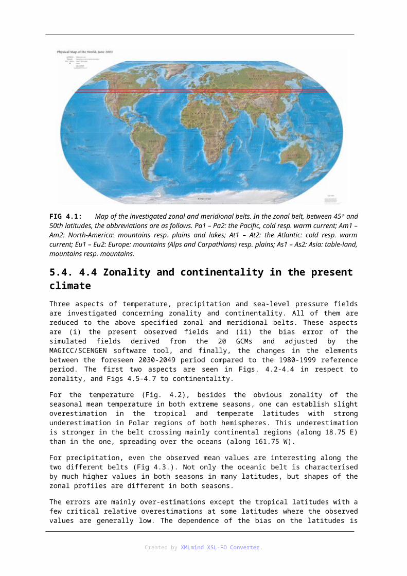
5. 4. Zonality and continentality ............................................................................................... 445.1. 4.1 Global climate models ....................................................................................... 445.2. 4.2 The MAGIC/SCENGEN diagnostic model ...................................................... 455.3. 4.3 The selected belts ............................................................................................... 465.4. 4.4 Zonality and continentality in the present climate ............................................ 475.5. 4.5 Zonality and continentality in the projected changes ....................................... 505.6. 4.6 Weathering: a complex effect of climate .......................................................... 52

Created by XMLmind XSL-FO Converter.

6. 5.On correlation of maize and wheat yield with vegetation index ....................................... 546.1. 5.1 Vegetation index ............................................................................................... 546.2. 5.2 Yield data .......................................................................................................... 556.3. 5.4 Correlation of yield with previous NDVI .......................................................... 586.4. 5.5 Using vegetation indices for objective regionalization ..................................... 61

7. 6. Solar energy resources ..................................................................................................... 627.1. 6.1. Data and methods ............................................................................................. 627.2. 6.2 Validation of global radiation grid-point data .................................................... 637.3. 6.3 Area-mean daily statistics .................................................................................. 64

7.3.1. 6.3.1 Averages ............................................................................................ 647.3.2. 6.3.2 Standard deviations of the diurnal values .......................................... 64

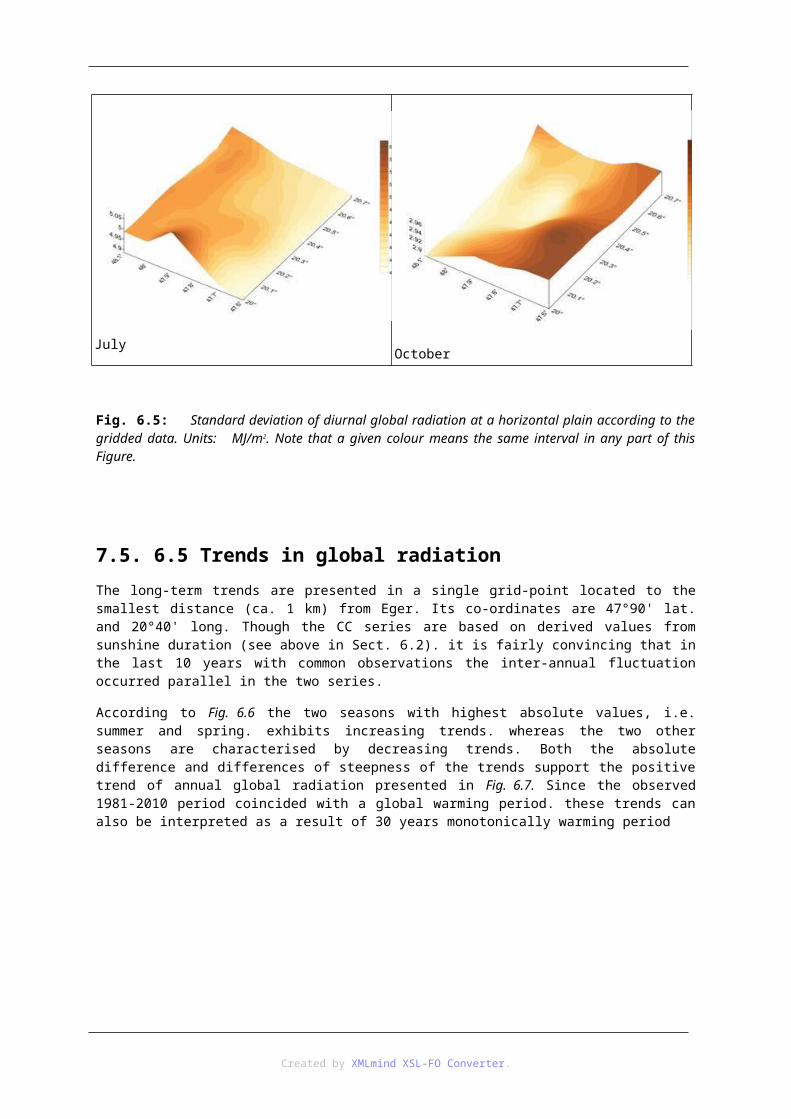
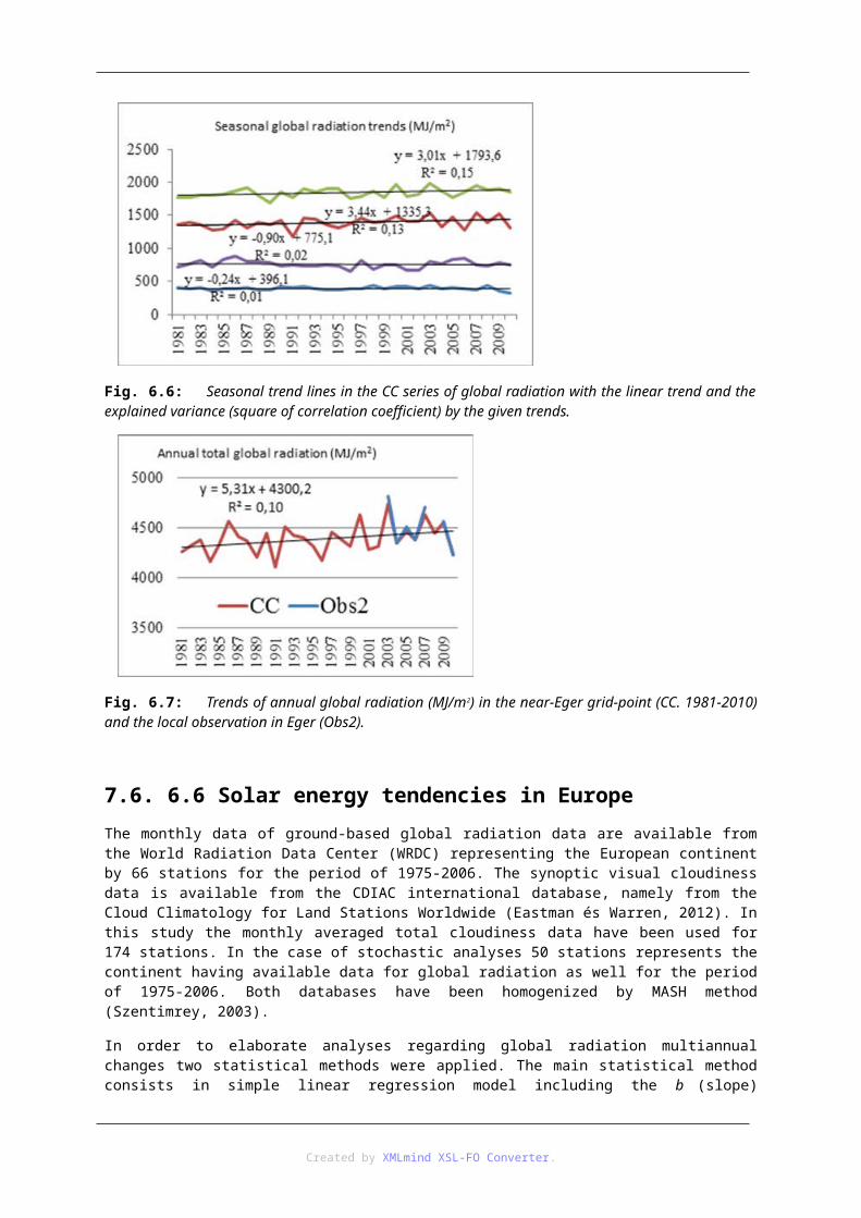
7.4. 6.4 Mapping the diurnal means and standard deviations ......................................... 657.5. 6.5 Trends in global radiation .................................................................................. 677.6. 6.6 Solar energy tendencies in Europe ................................................................... 68

7.6.1. 6.6.1 Changes in global radiation ................................................................ 687.6.2. 6.6.2 Changes in cloudiness ........................................................................ 697.6.3. 6.6.3 Relation between changes in global radiation and cloudiness ........... 707.6.4. 6.6.4 Conclusions for Europe ...................................................................... 71

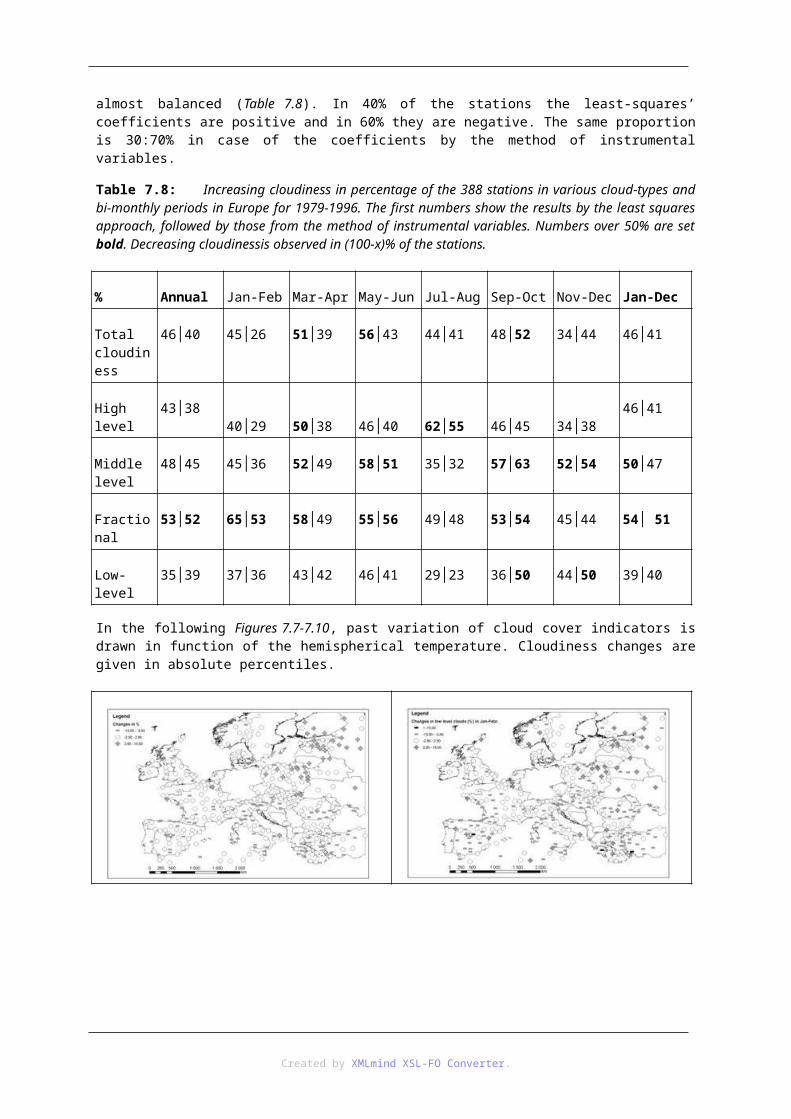
8. 7. Precipitation and cloudiness tendencies in the upper Danube catchment and in Europe 718.1. Fig. 7.1: Possible meanings starting from world scenario according to MS Word (1997) list of synonyms. Green set words are primary synonyms of ”scenario”, violet words are selected synonyms related to the primary ones. 7.1 Methods of investigation .............. 72

8.1.1. 7.1.1 Fourier analysis .................................................................................. 728.1.2. 7.1.2 Method of instrumental variables ...................................................... 73

8.2. 7.3 Annual cycle of precipitation ............................................................................ 748.3. 7.5 Effect of warming on cloudiness and sea-level pressure ................................... 788.4. 7.5 Broader analysis of trends in cloudiness .......................................................... 80

8.4.1. 7.5.1 Data for analysis ................................................................................. 808.4.2. 7.5.2 Statistical methods ............................................................................. 818.4.3. 7.5.3 Spatial distribution of the trends ........................................................ 81

9. 8. Analysis of precipitation and runoff in the Eastern Carpathians ...................................... 859.1. 8.1. The runoff data .................................................................................................. 869.2. 8.2. Parallel precipitation data ................................................................................ 879.3. 8.3. Basic statistics and extremities ......................................................................... 879.4. 8.4 Regression to the hemispherical temperature .................................................... 899.5. 8.5 Independent estimations .................................................................................... 929.6. 8.6 Behaviour of the absolute extremes ................................................................... 93

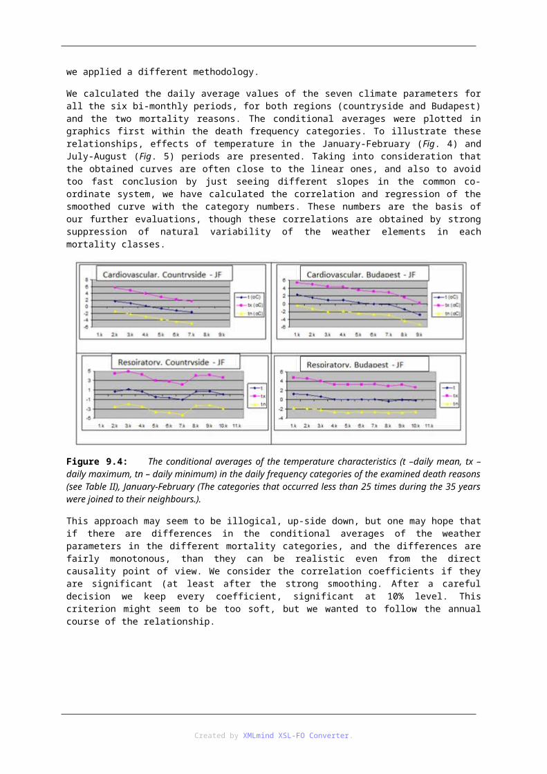
10. 9. Effect of local weather on human mortality .................................................................. 9510.1. 9.1 Mortality data, their trend and annual cycle .................................................... 9510.2. 9.2 The selected weather parameters .................................................................... 9710.3. 9.3 Methodology of the comparison ...................................................................... 9710.4. 9.4 Correlation of death rates with weather variables ........................................... 99

11. 10. Climate scenarios by various methods ....................................................................... 10411.1. 10.2 Methods providing extreme index scenarios ............................................... 106

11.1.1. 10.2.1 General Circulation Models ......................................................... 10611.1.2. 10.2.2 Mezoscale models ....................................................................... 10611.1.3. 10.2.3 Empirical regression ................................................................... 10611.1.4. 10.3 Comparison of changes in the local averages ................................. 106

11.2. 10.4 Comparison of selected weather extremes .................................................. 10711.3. 11.1 Introduction .................................................................................................. 11211.4. 11.2 Specifics of remote sensing in climate science ............................................ 113

12. 12. Satellite observations for climate science. Part II. ..................................................... 125


12.1. 12.1 Testing of climate reproduced by models .................................................... 12512.2. 12.2 Testing of climate model sensitivity ............................................................ 12612.3. 12.3 Effects of documented land use changes in Hungary .................................. 128

12.3.1. 12.3.1 Albedo estimation methodology ................................................ 12912.3.2. 12.3.2 Regional specification .................................................................. 13212.3.3. 12.3.3 Land-use series ............................................................................ 13212.3.4. 12.3.4 Area weighting ............................................................................. 13412.3.5. 12.3.5 Surface albedo tendencies ............................................................ 134

12.4. 12.4 Does climate system respect the GAIA-hypothesis? .................................. 13713. References: ....................................................................................................................... 13814. Matzarakis, A.; Mayer, H. and Iziomon, M. G., 1999: Applications of a universal thermal index: physiological equivalent temperature. Int. J. Biometeorology 43: 76-84 .............................. 14115. Oke, T. R., 1979: Boundary Layer Climates. John Wiley and Sons, 372 pp. .................. 14216. van Engelen, A., A. Klein Tank, G. van de Schrier and L. Klok, 2008: Towards an operational system for assessing observed changes in climate extremes European Climate Assessment & Dataset (ECA&D) Report, KNMI, De Bilt, Netherland, 70 p. ........................................................... 14417. Animations ....................................................................................................................... 14418. Films ................................................................................................................................ 144


ATMOSPHERE AS RISK AND RESOURCE

by Prof. Dr. János MIKA

Eszterházy College, Eger, Hungary

This course is realized as a part of the TÁMOP-4.1.2.A/1-11/1-2011-0038 project.

1. 1. Time and space scales1.1. Extreme weather


Specific concern at the middle latitudes are caused by thunderstorms, tornadoes, hail, dust storms and smoke, fog and fire weather. These small-scale severe weather phenomena, that are sparse in space and time, may have important impacts on societies, such as loss of life and property damage. Their temporal scales range from minutes to a few days at any location and typically cover spatial scales from hundreds of meters to hundreds of kilometres. These extremes are accompanied with further hydro-meteorological hazards, like floods, debris and mudslides, storm surges, wind, rain and other severe storms, blizzards, lightning. For example, mudslides disrupt electric, water, sewer and gas lines. They wash out roads and create health problems when sewage or flood water spills down hillsides, often contaminating drinking water. Power lines and fallen tree limbs can be dangerous and can cause electric shock. Alternate heat sources used improperly can lead to death or illness from fire or carbon monoxide poisoning.

Extreme events are often the consequence of a combination of factors that may not individually be extreme in and of themselves. Complex extreme events are often preconditioned by a pre-existing, non-extreme condition, such as the flooding that may result when there is precipitation on frozen ground. In addition, non-climatic factors often play a role in complex extreme events, such as air quality extremes that result from a combination of high temperatures, high emissions of smog precursors, and a stagnant circulation. Very often there is a possibility to predict quite accurately the probability of severe weather events and issue warnings, or even close the endangered region temporarily. But, tourists often do not speak the language of the country in which they are spending vacation. They do not know the local signs of danger and some of them do not respect warnings and prohibitions to enter the endangered areas.

Hence, characteristics of what is called extreme weathermay vary from place to place in an absolute sense. The professional surface-based observations of the Global Observing System provide weather measurements, including air temperature, wind speed, wind direction, precipitation, cloud cover, humidity, sunshine hours and visibility, etc. taken regularly over the Globe. Firstly, we list the extreme weather events following the so called synoptic codes, which indicate the events worth observing, forwarding to the prediction centers and archiving.

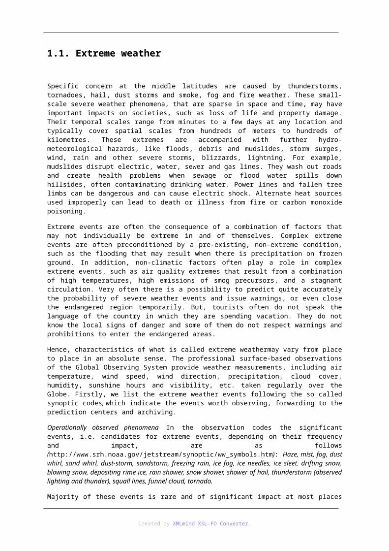
Operationally observed phenomena In the observation codes the significant events, i.e. candidates for extreme events, depending on their frequency and impact, are as follows (http://www.srh.noaa.gov/jetstream/synoptic/ww_symbols.htm): Haze, mist, fog, dust whirl, sand whirl, dust-storm, sandstorm, freezing rain, ice fog, ice needles, ice sleet. drifting snow, blowing snow, depositing rime ice, rain shower, snow shower, shower of hail, thunderstorm (observed lighting and thunder), squall lines, funnel cloud, tornado.

Majority of these events is rare and of significant impact at most places of the world. This may depend on severity of the event, which is in some cases well classified. Considering the low frequency but negative effects of icing, this event is a meteorological extreme in most regions in the world.

Another group of extremes is the appearance of continuous thermodynamic state indicators above or below a certain frequency and/or impact threshold, e.g. temperature below zero, or rainfall above 20 mm. These extremities are comprehended in the next sub-section.

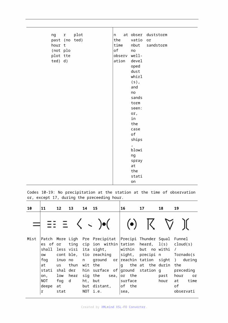
1.2. 1.2 Present Weather Symbols (http://www.srh.noaa.gov/jetstream/synoptic/ww_symbols.htm): In this Section the 100 weather symbols will be presented in Table 1.1.

Table 1.1: The 100 present-weather symbols of meteorology are divided into groups.

Codes 00-09: No precipitation, fog, duststorm, sandstorm, drifting or blowing snow at the station at the time of observation or, except for 09 during the preceding hour.

00 01 02 03 04 05 06 07 08 09


Cloud development NOT observed or NOT observable during past hour (not plotted)

Clouds generally dissolving or becoming less developed during past hour (not plotted)

State of sky on the whole unchanged during past hour (not plotted)

Clouds generally forming or developing during past hour (not plotted)

Visibility reduced by smoke

Haze

Widespread dust in suspension in the air, not raised by wind at or near the station at the time of observation

Dust or sand raised by the wind at or near the station at the time of the observationbut no well-developed dust whirl(s), and no sandstorm seen: or, in the case of ships, blowing spray at the station

Well developed dust whirl(s) or sand whirl(s) seen at or near the station during the preceding hour or at the time of observation, but no duststorm or sandstorm

Duststorm or sandstorm within sight at the time of observation, or at the station during the preceding hour

Codes 10-19: No precipitation at the station at the time of observation or, except 17, during the preceeding hour.

10 11 12 13 14 15 16 17 18 19

Mist Patches of shallow fog at station, NOT deeper than 6 feet on land

More or less continuous shallow fog at station, NOT deeper than 6 feet

Lighting visible, no thunder heard

Precipitation within sight, but NOT reaching the ground

Precipitation within sight, reaching ground or the surface of the sea, but distant, i.e. estimated to be more than 3 miles from the station

Precipitation within sight, reaching the ground or the surface of the sea, near to (within 3 miles), but not at the station

Thunder heard, but no precipitation at the station

Squall(s) within sight during past hour

Funnel cloud(s) / Tornado(s) during the preceding hour or at time of observation


on land

Table 1.1 cont.

Codes 20-29 General Group: Precipitation, fog, ice fog, or thunderstorm at the station during the preceeding hour but not at the time of observation.

20 21 22 23 24 25 26 27 28 29

Drizzle (not freezing) or snow grains not falling as shower(s) ended in the past hour

Rain (not freezing) not falling as shower(s) ended in the past hour

Snow not falling as shower(s) ended in the past hour

Rain and snow or ice pellets not falling as shower(s) ended in the past hour

Freezing drizzle or freezing rain not falling as shower(s) ended in the past hour

Shower(s) of rain ended in the past hour

Shower(s) of snow, or of rain and snow ended in the past hour

Shower(s) of hail, or of rain and hail ended in the past hour

Fog or ice fog ended in the past hour

Thunderstorm (with or without precipitation) ended in the past hour

Codes 30-39 General Group: Duststorm, sandstorm, drifting or blowing snow.

30 31 32 33 34 35 36 37 38 39

Slight or moderate duststorm or sandstorm (has decreased during the preceding hour)

Slight or moderate duststorm or sandstorm (no appreciable change during the preceding hour)

Slight or moderate duststorm or sandstorm (has begun or increased during the preceding hour)

Severe duststorm or sandstorm has decreased during the preceding hour

Severe duststorm or sandstorm has no appreciable change during the preceding hour

Severe duststorm or sandstorm has begun or increased during the preceding hour

Slight or moderate drifting snow (generally below eye level)

Heavy drifting snow (generally below eye level)

Slight or moderate blowing snow (generally above eye level)

Heavy drifting snow (generally above eye level)

Table 1.1 cont.

Codes 40-49 General Group: Fog at the time of observation.

40 41 42 43 44 45 46 47 48 49


Fog at a distance at the time of observation, but not at the station during the preceding hour, the fog or ice fog extending to a level above that of the observer

Fog in patches

Fog sky visible (has become thinner during preceding hour)

Fog sky obscured (has become thinner during preceding hour)

Fog sky visible (no appreciable change during the preceding hour)

Fog sky obscured (no appreciable change during the preceding hour)

Fog sky visible (has begun or has become thicker during the preceding hour)

Fog sky obscured (has begun or has become thicker during the preceding hour)

Fog, depositing rime ice, sky visible

Fog, depositing rime ice, or ice fog, sky obscured

Codes 50-59 General Group: Drizzle.

50 51 52 53 54 55 56 57 58 59

Drizzle, not freezing, intermittent (slight at time of observation)

Drizzle, not freezing, continuous (slight at time of observation)

Drizzle, not freezing, intermittent (moderate at time of observation)

Drizzle, not freezing, continuous (moderate at time of observation)

Drizzle, not freezing, intermittent (heavy at time of observation)

Drizzle, not freezing, continuous (heavy at time of observation)

Drizzle, freezing, slight

Drizzle, freezing, moderate or heavy

Drizzle and rain, slight

Drizzle and rain, moderate or heavy

Table 1.1 cont.

Codes 60-69 General Group: Rain.

60 61 62 63 64 65 66 67 68 69

Rain, not freezing, intermitte

Rain, not freezing, continuou





Rain, freezing, slight

Rain, freezing, moderate

Rain or drizzle and snow,

Rain or drizzle and snow,


nt (slight at time of observation)

s (slight at time of observation)

nt (moderate at time of observation)

s (moderate at time of observation)

nt (heavy at time of observation)

s (heavy at time of observation)

or heavy slight moderate or heavy

Codes 70-79 General Group: Solid precipitation not in showers.

70 71 72 73 74 75 76 77 78 79

Intermittent fall of snowflakes (slight at time of observation)

Continuous fall of snowflakes (slight at time of observation)

Intermittent fall of snowflakes (moderate at time of observation)

Continuous fall of snowflakes (moderate at time of observation)

Intermittent fall of snowflakes (heavy at time of observation)

Continuous fall of snowflakes (heavy at time of observation)

Ice needles (with or without fog)

Snow grains (with or without fog)

Isolated star-like snow crystals (with or without fog)

Ice pellets (sleet)

Table 1.1 cont.

Codes 80-89 General Group: Showery precipitation, or precipitation with current or recent thunderstorm.

80 81 82 83 84 85 86 87 88 89

Rain shower(s), slight

Rain shower(s), moderate or heavy

Rain shower(s), violent

Shower(s) of rain and snow mixed, slight

Shower(s) of rain and snow mixed, moderate or heavy

Snow shower(s), slight

Snow shower(s), moderate or heavy

Shower(s) of snow pellets or small hail, slight with or without rain or rain and snow mixed

Shower(s) of snow pellets or small hail, moderate or heavy with or without rain or rain and snow mixed

Shower(s) of hail, with or without rain or rain and snow mixed, not associated with thunder, slight

Codes 90-99 General Group: Showery precipitation, or precipitation with current or recent thunderstorm.

90 91 92 93 94 95 96 97 98 99


Shower(s) of hail, with or without rain or rain and snow mixed, not associated with thunder, moderate or heavy

Thunderstorm during the preceding hour but not at time of observation with slight rain at time of observation

Thunderstorm during the preceding hour but not at time of observation with moderate or heavy rain at time of observation

Thunderstorm during the preceding hour but not at time of observation with slight snow, or rain and snow mixed, or hail at time of observation

Thunderstorm during the preceding hour but not at time of observation with moderate or heavy snow, or rain and snow mixed, or hail at time of observation

Thunderstorm, slight or moderate, without hail but with rain and or snow at time of observation

Thunderstorm, slight or moderate, with hail at time of observation

Thunderstorm, heavy, without hail but with rain and or snow at time of observation

Thunderstorm combined with duststorm or sandstorm at time of observation

Thunderstorm, heavy, with hail at time of observation

In Fig. 1.1 One can see the most important symbols around the station, taken from the same Internet source as Tab. 1.1: http://www.srh.noaa.gov/jetstream/synoptic/ww_symbols.htm

Figure 1.1: Symbols drawn around a station on the weather maps.

The weather observations, together with above surface observations and intensive observing systems (e.g radiosouns, satellites, etc. see in the animations) are important themselves, however they provide initial state data for the weather forecasting equations. The latter ones are partial differential equations, representing the physical laws of conservation for mass, thermodynamic energy and momentum (Fig 1.2)


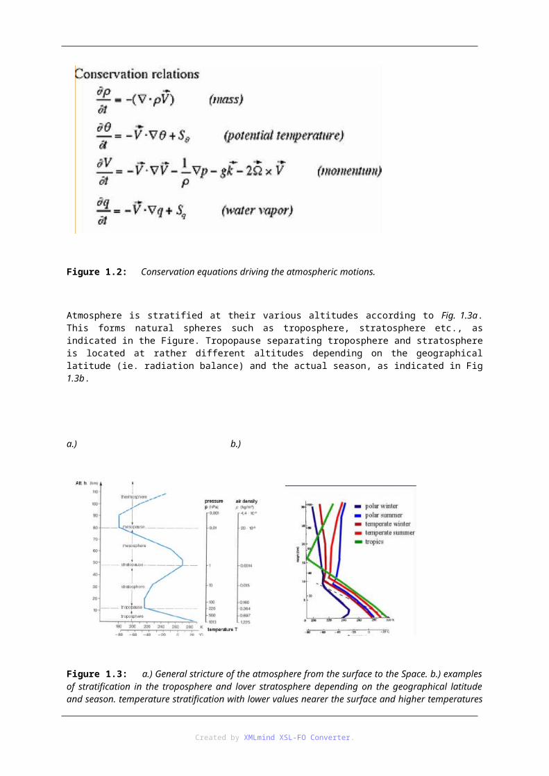
Figure 1.2: Conservation equations driving the atmospheric motions.

Atmosphere is stratified at their various altitudes according to Fig. 1.3a. This forms natural spheres such as troposphere, stratosphere etc., as indicated in the Figure. Tropopause separating troposphere and stratosphere is located at rather different altitudes depending on the geographical latitude (ie. radiation balance) and the actual season, as indicated in Fig 1.3b.

a.) b.)

Figure 1.3: a.) General stricture of the atmosphere from the surface to the Space. b.) examples of stratification in the troposphere and lover stratosphere depending on the geographical latitude and season. temperature stratification with lower values nearer the surface and higher temperatures above it is called (thermal) inversion.


1.3. 1.3 Time and space scalesAtmospheric objects exhibit fairly arranged space and time scales. Either drawing the meteorological extremes in the space (x-axis) and time (y-axis) system of coordinates (Fig. 1.4a), or doing the same with the atmospheric objects (Fig. 1.4b), we observe a diagonal distribution of the objects of both drawings. This means, small scale objects are generally short lived, whereas large-scale objects spend more time in the atmosphere.

On the other hand it also means that there are no fast developing extremes which cover large areas and also we do not experience long-term individual extremes or objects which threaten just small areas. Fig 1.4a provides a comprehensive list of meteorological extremes, whereas Fig 1.4b is a brief summary of the atmospheric objects leading to the various meteorological extremes.

a.) b.)

Figure 1.4: Characteristic space (horizontal) and time (vertical) scales of a.) weather and climate extremes and b.) atmospheric objects. Sources: a.) Golnaraghi M., 2005, (2006), b.) Oke, 1979.

Weather extremes are immediately caused by specific weather objects. In developing climate extremes circulation processes also play well recognized role. In the following we briefly survey these objects from the largest scale blocking anticyclones to the smallest scale convective systems. Besides these individual objects, there are even longer-time patterns of the circulation, like the El-Nino - Southern Oscillation or North Atlantic Oscillation, which are not individual circulation objects themselves, but which support specific objects to develop.

For example, unusually warm water surfaces in case of an El-Nino event support developing low-pressure systems above the ocean, and, via complex dynamical processes, higher pressure systems above the continent,.


Though long-term climate extremes can statistically be correlated with these objects, we do not characterize these planetary-scale derived indices below.

Anticyclones generally bear pleasant sunny weather, with no strong air motions, but long residence time above a given land area may lead to drying or even drought of the area. The larger the anticyclones are in their horizontal dimensions, the longer their life-time and slower their transition are. The so called blocking anticyclones of the temperate latitudes may remain for several weeks practically in the same position. Having several such objects in a vegetation season may already cause drought.

Temperate latitude cyclones, as large-sale objects, already bear threats of heavy precipitation and strong gradient winds. Warm fronts of temperate latitude cyclones are responsible for low-intensity, but several days’ long precipitation. Cold fronts of the cyclones may yield large amount and large intensity precipitation. Convective activity in and around the cold front, caused by upward motion of relatively warm air masses, may enhance the gradient wind sometimes causing extremely strong wind.

Convection is a key to extreme weather events. Starting from small cumulus clouds, possibly developing into single-cell local thunderstorms, they are still not subjects of extremes events. Multi-cell thunderstorms, causing heavy rain, sometimes hail and stormy wind are already extremity-bearing atmospheric objects. Single-cell thunderstorms sometimes develop into super-cells, accompanied with devastating wind and hail, heavy rain and often even with tornado. Not so dangerous, but more complicated are the so called mezoscale convective complexes (MCC), often bearing thunderstorm lines, squall lines, characterized by stormy wind, hail and intensive rain.

The most devastating objects of convective origin are the hurricanes (tropical cyclones, typhoons). Their 3-500 km characteristic diameter develops after a large number of coincidental conditions leading to accumulation of very high amounts of available potential energy turning into kinetic energy. In a tropical cyclone, extremely strong winds, intensive rain and hail, with several meters high waves at the shores cause infinite harm.

1.4. 1.4 Climate extremesClimate extreme is a longer-term mean or frequency of variables or events, even if the latter are not weather extremes, which are rare at the given site in the given time of the year, and which are of potentially high impact. The climate extremes may be time averages or frequencies of events above a given threshold of a single meteorological variable. These indices are presented below. Those extremes which occur in the multi-dimensional phase-space, but which are mostly transformed into univariate indices, are illustrated afterwards.

Univariate indices. Typical indices include the number or fraction of cold/warm days/nights etc. above the 10th percentile, generally defined with respect to a preselected reference period. Other definitions e.g., the number of days above specific temperature or precipitation thresholds, or those related to the length or persistence of climate extremes.

Table 1.2: Selected examples from the 40 univariate climate indices used in ECA&D. (see http:// eca.knmi.nl/indicesextremes for details, van Engelen, et al., 2008).

Index Climate Index Description

TG, TN and TX

Mean of daily mean, maximum and minimum temperature (°C)

(For further use in the indices)

ETR Intra-period extreme temperature range (°C)

Difference: max(TX)- -min(TN)

GD4 Growing degree days (°C) Sum of TG > 4°C

GSL Growing season length (days) Count of days between first span of min. 6 days TG > 5°C and first span in second half of the year of 6 days TG < 5°C


CFD Consecutive frost days (days) Maximum number of consecutive days TN < 0° C

HD17 Heating degree days (°C) Sum of 17°C - TG

ID Ice days Number of days TX < 0°C

CSFI Cold spell days (days) Number of days in intervals of at least 6 days with TG < 10percentile calculated for each calendar day (on basis of 1961-90) using running 5 day window

WSDI Warm spell days (days) Number of days in intervals of at least 6 days with TX > 10percentile calculated for each calendar day (on basis of 1961-90) using running 5 day window

TN10p Cold nights(days) Percentage or number of days TN < 10percentile calculated for each calendar day (on basis of 1961-90) using running 5 day window

TG90p Warm days (days) Percentage or number of days TG > 90percentile calculated for each calendar day (on basis of 1961- 90) using running 5 day window

RR Precipitation sum (mm)

RR1 Wet days (days) Number of days RR ≥ 1 mm

SDII Simple daily intensity index (mm/wet day)

Quotient of amount on days RR ≥ 1mm and number of days RR ≥ 1mm

CDD Consecutive dry days (days) Maximum number of consecutive dry days (RR < 1mm)

R20mm Very heavy precipitation days (days) Number of days RR ≥ 20mm

RX1day Highest 1-day precipitation (mm) Maximum RR sum for 1 day interval

R95p Very wet days (days) Number of days RR > 95percentile calculated for wet days (on basis of 1961-90)

R95pTOT Precipitation fraction due to very wet days (%)

Quotient of amount on R95percentile days and total amount

In 1998, a joint WMO-CCl/CLIVAR Working Group formed on climate change detection. One of its task groups aimed to identify the climate extreme indices and completed a climate extreme analysis over the world where appropriate data was available. Extreme climate analyses have been accomplished on global and European scales using these compiled datasets. A selection of these indices is given in Tab. 6.1 already from a more recent source using 40 indices (van Engelen et al., 2008).

Multivariate extremities, transformed into univariate indices. Extremity of weather or climate, as well as the effect of them are often more complex than rarity or severity of one single meteorological variable. The use more variables, however, does not allow to establish a linear sequence of the extremities. Hence, most often the multivariate extremities are arranged into a single index.

For example, the thermal comfort index is calculated by means of the physiologically equivalent temperature, PET, based at the human energy balance (Matzarakis et al., 1999). For calculating this weather


extreme four meteorological parameters (air temperature, relative humidity, wind speed and cloudiness) as well as some assumed physiological parameters (age, genus, bodyweight and height, average clothing and working) are used.

Our second example on multivariate indices is related to a climate extreme, drought, which is possibly the most slowly developing one. There are many conceptual definitions of drought in the scientific literature. Recently, Dunkel (2009) collected a few of them focusing on the more practical indices from data accessibility point of view. A very commonly used and accepted index is the Palmer Drought Severity Index (Alley, 1984), which considers monthly precipitation, evapotranspiration, and soil moisture conditions.

See also the ANIM_1_1 with the various observation networks and ANIM_1_2 with a series of radar images from a long series of days with precipitation.

FILM_1_1_cloud_webcam.avi presents cloud movements as seen from the surface by a web-camera and from the space by the Meteosat geostationary satellite. The webcameras are operated by the Hungarian Meteorological Service (OMSz).

FILM_1_2_bootcloud_Italy.mpeg provides a unique set af moving satellite images effectively illustrating that cumulus cloudiness is primarily generated by convection. These clouds form exclusively over the hot Apennine peninsula over Italy in the given situation, but not over the cool sea surface around it.

2. 2. Limitations of macro-circulation objects(Can water deficits of Lake Balaton in 2000-2003 be explained by circulation anomalies?)

This Section presents a quantitative analysis answering the question put in the brackets. After general exposition of the problem (Section 2.1), the methodological bases of this effort are given in Section 2.2, whereas the quantitative explanation is described and illustrated in Section 2.2. Finally, lack of success in explaining the missing precipitation and assumed consequences related to macro-circulation based statistical downscaling are discussed (Section 2.3).

2.1. 2.1 General expositionExtreme weather and climate events received increased attention in the last few years,due to the loss of human life and exponentially increasing costs, associated with them (Changnon et al., 1996). At the temperate latitudes, major extremes are connected with irregular water supply of land surfaces by precipitation. Both, flooding or inundation and drought may cause serious damage in hydrological and agricultural objects and values.

Precipitation is connected mainly with mezo-scale atmospheric phenomena and influenced by physical processes of smaller dimensions, including microphysics of cloud droplets and crystals. Hence, deterministic computation of this atmospheric variable is rather limited compared to requirements of medium-range weather forecasts and climate scenarios.

Statistical approaches to derive precipitation fields from synchronous circulation patterns were first applied in medium-range weather forecasting (Glahn and Lowry, 1972; Klein and Glahn, 1974), and later in regional down-scaling (e.g. Bardossy et al, 1995). Both applications are based on the common sense that pressure or geo-potential fields can be better predicted by the models, than the short lived precipitation objects. This approach is also useful if one combines daily circulation types with point-wise conditional distributions of precipitation (Bartholy et al., 1995), where patterns are likely better approached, too.

In Europe the cyclone tracks established by van Bebber are presented in Fig. 2.1. Track I is busy in all seasons. Tracks II and III are engaged mainly in winter, whereas the track 4 make weather forecastersbexcited mainly in summer and autumn. Track V/a delivers cyclones mainly in winter, whereas the track V/b, crossing northward through the region of the Carpathian Basin is mostly engaged in spring and in October. The frequency list is led by track I, where 31 % of the cyclones move along in winter and 39 % in summer. Further positions are taken by tracj IV (12 and 22 %) and track V (13-18%).


Figure 2.1: Cyclone tracks in Europe (after Van Bebber)

2.2 Methoology

2.1.1. 2.2.1 Statistical assessment using circulation types

In the followings, a method is introduced to calculate the relative contribution of the circulation anomalies, expressed by frequency distribution among finite number of classes, to the climate anomalies. The aim of this method is to quantify what part of climate anomalies can be directly attributed to the anomalous frequency distribution of macro-synoptic types in the period for which the anomaly is formed. Mathematical formulation of this task is as follows:

Let a mark the deviation of diurnal precipitation from its climatic mean in a preliminarily fixed period consisted of M days (e.g. M=30 for monthly, or 90 for seasonal periods). Let us further have k different circulation types, one of them unequivocally being valid at each day of the investigation period. It is also possible to identify the

deviation of the frequency related to the j-th circulation type from its climatic average frequency. If having a longer period of diurnal precipitation and also of circulation type series, it is also possible to compute the sign and the amount the conditional precipitation differs from the overall diurnal average in the given period

of the year. This average conditional anomaly of precipitation, , can be computed as follows:

. (1)

If the precipitation anomaly of the given period of M days is largely caused by anomalous occurrence of the circulation types, then the observed anomaly, a, and the above anomaly of circulation origin, a*, are of similar value. Earlier investigations, based on different subjective and objective classifications and various target variables for Hungary, established, however, that this circulation term was able to explain just a minor part of the monthly anomalies (Mika, 1993, Mika et al., 2005). On the other hand, according to both papers, the circulation term and the overall anomaly fluctuate in strong correlation with each other.

In the followings terms, a and a*, are compared by using three different classifications described in the following section. Bimonthly periods (Jan-Feb, Mar-Apr, etc.) are investigated considering four consecutive years, 2000-2003. This separation of the months ensures separate treatment of the primary (May-June) and the secondary (November-December) precipitation maxima of the year. For reference period we used the period 1990-1999.


2.1.2. 2.2.2 The applied classifications

Macro-synoptic classification is a description of spatial distribution of the sea level pressure or mid-tropospheric geopotential height by subjective or objective methods. In the followings, the three applied subjective classifications are briefly described. The three classifications are listed in a decreasing order of their spatial scope.

2.1.3. 2.2.2.1 Hess-Brezowsky classification, amalgamated (9 types)

The Hess-Brezowsky (HB) classification (Hess and Brezowsky, 1969), based on the diurnal sea-level and mid-troposphere pressure fields of Central Europe, scoped from Germany, defines 29 different types and allows one class for the rare undefined patterns. The HB-codes are defined operatively by the German Weather Service in Frankfurt am Main. Actually, this coding was used until the end of 2001, but from 2002 the operational coding by the Hungarian Meteorological Service was applied in the calculations.

This number of classes, however, is too large for our purposes and sample sizes. Hence, they are objectively compressed into 9 groups, considering the results of a factor analysis (von Storch and Zwiers, 1999), performed for the annual sea-surface pressure maps averaged for each of the 29 HB types (Mika et al., 1999). These maps had previously been derived by Bartholy and Kaba (1987), who collected diurnal pressure patterns of a 11 years period, and determined average annual mean sea-surface pressure distribution above the continental Europe (2.5 x 2.5 rectangles), i.e. above the area of the HB classification.

Reduction of the HB types is performed by factor analysis of the 30 average pressure patterns. Number of retained factors is determined by the Guttman criterion (Bartzokas and Metaxas, 1993), to keep the factors with eigenvalues>1. Rotation of the axes (factors) is performed by Orthogonal Varimax Rotation, which keeps the factors uncorrelated. This process achieves discrimination among the loadings, that makes the rotated axes easier to interpret.

Number of eigenvectors to retain was definitely four, but cases (i.e. original HB-types) with opposite signs (cyclone, or anti-cyclone above a large of the map) were kept different in the new cumulated classification. Some cases not unequivocally separated by the factors also occurred, but (the rotated) Factor 3 contributed to each of them with high positive or negative loading. The original unclassified cases are kept separately, though its frequency is rather low.

This methodology contributed to the reduction of the number of macro-types from 30 to 9. Tab. 2.1 demonstrates the new, condensed macro-types. The correspondence between the original and the condensed types is established objectively, without any further synoptic consideration. To follow this correspondence, one could turn to the original paper by Hess and Brezowsky (1969), or to any paper applying this classification (e.g. Bartholy et al., 1995).

Tab. 2.1: Amalgamation of the 29 primaryHess-Brezowsky types into 9 different classes, according to factor analysis of the mean sea-level pressure patterns (Mika et al., 1999)

Classes Class 1. Class 2. Class 3. Class 4. Class 5. Class 6. Class 7. Class 8. Class 9.

Factors F1: + F2: + F3: + F4: + F1: - F2: - F2-F3:+ F3: - EXTRA

Original HB-types

Sa Sz, SEa Sez, HFz TM

Wa SWa

HM BM

Ws Ww TB TRM TRW

NEa NEz HFa

Na Nz NWa

NWz

HNz HNFz

Wz SWz HB HNa HNFa

Egyéb


2.2.2.2 Péczely classification (13 types)

Considering weather situations in Hungary, Péczely (1957) defined a macro-synoptic classification, based on the position of cyclones and anticyclones on the sea-level pressure maps. Thirteen types are separated and grouped according to direction of the prevailing current (Tab. 2.2). The types consider the position of the major frontal systems relative to Hungary, as well. Transition-probability matrices of the different types are given by Péczely (1983) for 1881-1983. Since his death, Karossy (1987 and updated) continues the tradition, determining the actual codes, with the intention to repeat the original macro-circulation identification.

2.2.2.3 Bodolainé classification (8 types)

The aim of the monograph, written by Bodolainé (1983), is to establish the synoptic conditions of flood waves in the Danube and Tisza basins, describing the background of the genesis of floods in terms of synoptic-climatology. Weather types with enhanced precipitation activity are analysed, including their distribution in time and space, the watered area and the amounts.

Tab. 2.2: The 13 individual types of the Péczely (1957) macro-synoptic classification. (These types are used according to their serial numbers, i.e 1 for mCc, 2 for AB, …, 13 for type C. The related drawings of Figs. 2 and 3 are marked according to this rule.)

MERIDIONAL TYPES ZONAL AND CENTRAL TYPES

Types connected with westerly current:

Types connected with northern current: zC - zonal flow, slightly cyclonic influence

mCc - H is in the rear of a West-European cyclone Aw - anticyclone extending from the west

AB - anticyclone over the British Isles As - anticyclone to the south from Hungary

CMc - H is in the rear of a Mediterranean cyclone Types connected with easterly current:

An - anticyclone to the north from Hungary

Types connected with southerly current: AF - anticyclone over the Fenno-Scandinavia

mCw - H is in the fore of a West-European cyclone Types of pressure centres:

Ae - anticyclone to the east from Hungary A - anticyclone centre over Hungary

CMw - H is in the fore of a Mediterranean cyclone C - cyclone centre over Hungary

Tab. 2.3: The seven types of the Bodolaine (1983) classification with considerable precipitation. (Serial numbers assigned to the types are used in Fig. 3.)

. West-type-weather situations (W):

· a deep cyclone is situated over North-Europe at mean see level pressure

· strong westerly stream is characterised over the Carpathian basin at 500 and 700 hPa levels.


· the precipitable water is generally higher, than the average.

· The temperature is higher during winter, and cooler during summer.

2. West type with secondary lateral distribution (Wp):

· a deep cyclone is situated over the North-Sea at mean see level pressure

· strong south-westerly stream is over the Carpathian basin at 500 and 700 hPa levels.

· the precipitable water and the temperature is always higher, than the average all the year.

· This is a warm situation in the Carpathian basin.

3. Zonal-type weather situation (Z):

· a deep cyclone is situated relatively far over the North-Sea at mean see level pressure

· westerly stream is characterised over the Carpathian basin at 500 hPa level.

· Temperature is higher during winter and spring, causing snowmelt in the Alps in this period.

4. Transporting Mediterranean cyclone-type (M):

· a cyclone is situated near or over the Carpathian basin at mean see level pressure

· strong south-westerly stream is characterised over the Carpathian basin at 500 hPa levels

· the precipitable water is much more higher, than the average.

· Considerable part of the annual precipitation amount is connected with this type in Hungary.

5- Centrum-type weather situation (C):

· a deep cyclone over the Carpathian basin both at the see level and at the higher levels, as well

· the precipitable water is always higher, than the average all the year.

· It is a relatively rare situation, but it causes a lot of precipitation in the Carpathian basin.

6. West cyclone type weather situation (Cw):

· a deep cyclone over West Europe at higher level, and over the Alps at mean sea level pressure.

· the precipitable water and the temperature is always higher, than the average all the year.

· This is a warm situation in the Carpathian basin.

7. Cold air –drop weather situation (H):

· This situation is often during summer.

· The curvature of isobars is cyclonic in the Carpathian basin

· The unstable air and high precipitable water are favourable conditions for convective systems.

Classification of the weather-systems of the flood-waves producing rainfall periods can also be found in the monograph. The weather types are defined by the ridge- and trough-lines of the 500 hPa surface, by those of the 500/1000 hPa thickness, as well, as by the near-surface position of cyclones and anticyclones. These types can also be expressively characterised by the mean fields of the precipitable water. Seven circulation types characterised with significant precipitation in Hungary were defined (Tab. 2.3), plus another type without strong precipitation activity was also introduced: The catalogue of the weather types, regarding the period between 1951 and 1980, enabled also the frequency analysis of the types.


For the period after July 2001, the coding was performed by one of the authors (L.P.), performed using 00 UTC maps of 500 hPa and sea-level pressure, published by the German Weather Service web-site, www.wetterzentrale.de, also considering daily precipitation data.

2.1.4. 2.2.3 Point-wise vs. area-mean precipitation

Precipitation directly reaching the Lake Balaton surface is determined from ca. 10 stations, situated in close vicinity of the Lake. The same value for the whole water catchment is derived from ca. 25 stations. Our estimation of circulation component, described in Section 2.1, needs daily precipitation data, which were obtained only for one station, Siofok. Hence, the aim of the following paragraphs is to demonstrate close correlation and near-unity regression between monthly values of this single station, and those for the large areas, including the whole watershed and the lake, as well.

As indicated in Fig. 2.2, both statistical characteristics are fairly close to the unity. Each coefficient is derived from 10 pairs of data between 1990 and 1999. All correlation coefficients between the point-wise observations and the area-mean characteristics are above 0.8. (One should note that correlation between lake-mean and watershed-mean precipitation is not always 1, either.) The coefficients are somewhat higher between point-wise observations and lake-mean estimates, but in 4 months of the year (November, January, February and March) even this relation is the opposite.

Point-wise observations can be used for area mean estimates with regression coefficients that are, again, fairly close to the unity, Moreover, regression coefficients between point-wise observations and one or the other area-mean estimates do not deviate from the unity more than the same regression between the two area-mean estimates, themselves.

Hence, the single-station precipitation observations are considered to explain lack of water supply in the 2000-2003 period in comparison with the previous ten years, 1990-1999.

Fig. 2.2: Correlation and regression coefficients between precipitation falling to the water cathment and the single station (Siófok), between those captured by the lake and, again, the single station, and also between the catchment and the lake captured values. Each coefficient is derived from 10 pairs of data between 1990 and 1999.

2.3. Estimation of precipitation by macro-circulation

2.1.5. 2.3.1 Conditional mean precipitation

As expected, conditional mean precipitation considerably differs between the classes of a given classification.


This is valid for all the three above classifications (Fig. 2.3).

In case of the condensed HB-classification (Fig. 2.3a) the highest average precipitation sums are accompanied with classes 6, 3 and 4 (see in Tab. 1), representing the frontal section or the axis of a high-level trough with cyclonic curvature above the Carpathian basin. Not surprisingly, the lowest average precipitation occurs in Class 2, which bears mainly anticyclonic situations over Hungary.

For the Péczely-types (Fig. 2.3b) the highest average precipitation sums are accompanied with the cyclonic situations (class 6, 4, 13, 1, 7 and 6, see in Tab. 2.2). The highest amounts are accompanied with warm fronts of the Mediterranean and the Atlantic cyclones. Definitely lower amounts occur in the anticyclonic situations (class 12, 8, 10, 9, 5, 2 and 11, as ordered in the opposite direction).

The Bodolainé-classification (Fig. 2.3c) relates the highest average precipitation sums with transporting Mediterranean cyclones (type M, see in Tab. 2.3) and with three other types characterised by cyclonic curvature or effect of such areas on Hungary. Much lower amounts occur in the zonal types with no meridional disturbances in the region (types Z and W), and in the class “rest”, which is not considered to be significant from precipitation point of view.

To conclude this sub-section, one can establish that higher average precipitation is really connected with cyclonic types, but non-zero conditional averages occur even in the anticyclonic situations, as well.


Fig. 2.3: Mean conditional precipitation, according to the individual macro-synoptic types. 1990-2003, Siófok, Hungary. (Although in process of estimation monthly distinction among the conditional anomalies is performed, the present figures are annual averages.) Siófok, Hungary. (Although in the process of estimation monthly distinction among the conditional anomalies is performed, the presented figures are annual averages.)

2.1.6. 2.3.2 Frequency of the circulation types in 2000-2003 vs. 1990-1999

The other side of the question, put in the title of the paper, is how much the frequency distribution of the circulation types differed from its average one in the given four years. Parallel columns of Fig. 2.4 indicate these differences in bimonthly resolution. First columns always correspond to the 10-years mean frequency (1990-1999). The second ones represent the same 2 months of the critical four-year period (2000-2003) with lower than normal precipitation.

Fig. 2.4: Frequency of the given types in the three applied classifications. 10 J-F means January-February 1990-1999, and the next column to the right means the frequency distribution in the given four-year period of drought at Lake Balaton These columns can be analysed to establish quantitative differences between the 4-years and the 10-years periods. Of course, none of the three types exhibit identical distribution of the types in the two periods. For the most critical May-June period, when the lack of precipitation was the most serious, as compared to normal values, surplus of types with low precipitation and lower frequency of highest conditional means were observable. I.e., less frequency of types 3, 4 and 6, but more cases with type 5 can be


established in terms of the cumulated HB-types. The same in terms of Péczely classification means below normal frequency of wet types 3, 4 and 6, and above normal occurrence of dry types 5 and 12. Classification by Bodolainé exhibits far more non-significant (“remaining”) types, but less than normal frequency of types M and Cw.

2.1.7. 2.3.3 Observed vs. circulation-related anomalies of precipitation

Results of the estimation on effect of circulation, applying formula (3.1), are comprehended by Fig. 2.5. Comparison of the observed precipitation anomalies with those estimated by the three classifications, unequivocally point at the secondary role of the circulation factor.

Among the six bimonthly periods, January-February and July-August exhibit almost zero anomaly of precipitation during the four years. In these periods the circulation term does not differ much from the observed one. In the other four periods of the year, however, the observed anomalies are poorly approached by the circulation term. In the March-April and November-December periods even signs of the circulation term are positive, contrary to the considerable negative anomalies of the observed precipitation. In September-October the negative observed anomaly is paired by two small negative estimated anomalies (HB and Péczely types) and one larger positive one (Bodolainé types). Hence this estimation is not good either.

Sign of the anomalies is correctly reflected only in the most critical May-June period, with 1 mm/day negative anomaly (i.e. 60 mm/2 months, or 240 mm in the four May-June periods of 200-2003). But, even in this case, proportion between the real anomalies and the estimated ones is more than 2 for the Péczely and Bodolainé types, and more than 10 in case of the cumulated HB-types. This means, that even in this favourable case we can speak about qualitative indication of the negative anomaly by the circulation types, only. Larger part of the anomalies should be searched in other physical processes and, maybe, in smaller space scales.

Fig. 2.5: Results of bimonthly precipitation estimation, using the three circulation classifications (columns), and the observed precipitation at Siófok (line with the values) during 2000 and 2003. 2.4 Discussion

Although hydrological features of the 2000-2003 period induce a lot of questions, most important out of those is whether or not similar situations become more frequent in the future, as the global climate changes, our focus remains only on the question of circulation and precipitation. The main conclusion is that the missing precipitation of the years 2000-2003 can not be sufficiently explained by shifted frequency of the circulation types and conditional precipitation. This conclusion corresponds to all the three applied circulation


classifications. This is somewhat surprising, since HB-types and Péczely-types consider large-scale objects, only, but the Bodolainé classification, should have even better chances to capture the negative precipitation anomalies, since this classification was elaborated to estimate large precipitation.

Lack of successful precipitation estimation by frequency anomalies of the circulation types may be connected with two specific features of the classifications. Firstly, the subjective diurnal coding of the weather patterns into one of the classes is also a possible source of uncertainty that likely decreases the efficiency of attribution to circulation. This problem, parallel to the one mentioned below, indicate that there is still room for improvement in principle. This gives some hope to achieve better explanation of long-term anomalies, as it was important for various further applications, as well. One of them is downscaling of global climate changes. The second source of uncertainty is the lack of mezo-scale objects in the three classifications. In case of precipitation, this is possibly the most important shortcoming of the applied classifications, since this variable is directly related to this scale, as it is simply seen from its spatial and temporal variability (sporadic nature, weak spatial and temporal correlation, etc.). It is impossible, however, to consider the above use of circulation as the maximum information contained by the series of macrotypes. The succession of the macrotypes and conditional relation (physical adaptation) of local weather to the age of a given type above the region is not taken into account by the given estimation. E.g. cool and wet westerlies at the beginning of the period, followed by warm and dry anticyclones could cause different bi-monthly anomaly than the opposite case. For example, extraction of more information from series of macro-synoptic types, than just their frequency, was performed by Bartholy et al. (1995), who considered conditional auto-correlation under the given macro-type, as well.

On the other hand, a recent study (Mika et al., 2005) came to a negative conclusion concerning the maximum information represented by macro-circulation. This study applied one of the above classifications, the Péczely-types, for another station of Hungary. It was pointed out, that even if all possible information covered by these sequential features is subtracted, the part of anomalies falling out of the scope of macrosynoptic calendars remains of the same order of magnitude, as the anomalies, themselves. This means, one cannot avoid to deal with the physics of precipitation to find the reasons of low precipitation, even in case of the events of the past.

See also ANIM_2_1 which demonstrate the Kyrill temperate latitude cyclone causing rather serious problems in Europe. in January, 2007.

FILM_2_1_geostrophy.avi combines satellite images and radisonde observations on November 15, 2009. Clouds follow the large-scale patterns of isohypses at 400 hPa level. That day the movement was ideally geostrophical over Europe at that height.

FILM_2_2_cloud_scattering.avi indicates scattering of convective cloudiness over Hungary. This means that approaching to sunset (but still during the day, as visible satellite images are available) lack of convection allows thos fast process of the otherwise eveloped cloudeiness. (METEOSAT observations on June 29, 2009.)

3. 3. Effects of mezo-scalesSophisticated efforts to use GCM-outputs for regional climate scenario construction can be sorted into two groups. In both approaches, however, accuracy of the large-scale flow generated in the GCM is crucial. The first possibility is a one-way coupling of a limited-area model into the original sequence of GCM-fields. At present this approach is beyond the possibility of many research institutions due to its high demand in computer capacity and initialisation efforts.

The second way is to combine larger scale averages, or pattern components of the model-generated fields with empirical relationships, learned on measured data sets, between the large-scale characteristics and regional anomalies. In terminology of forecasters, this combination of model generated fields with empirical connections is a "perfect prognosis" approach. That is, a statistical model is developed between dynamic and prognostic quantities in the presently observed atmosphere, and it is applied to the simulated (future) atmosphere with no respect to the possible systematic deviation of the projected circulation patterns from the really occurring ones.

To test this approach, a method is introduced to calculate the relative contribution of macro-circulation anomalies, expressed by frequency distribution among finite number of classes, to the climate anomalies. After describing the method (Section 3.1), the applied objective macro-synoptic classification (Section 3.2) is introduced. Results are presented for monthly anomalies of five weather characteristics: precipitation, mean, maximum and minimum temperatures; and inter-diurnal change of mean temperature. The results are structured


according to the presented statistical characteristics. Section 3.3.1 demonstrates behaviour of moderate and extreme anomalies. Section 3.3.2 presents the standard deviations and Section 3.3.3 displays contribution of the terms to the long-term tendencies. Finally, Section 3.3.4 analyses the correlation between the components and their sum (i.e. the anomaly). Section 3.4 contributes to discussion on applicability of the macro-circulation types in statistical downscaling. Mezos-scale events, mostly created by convection are briefly presented in Section 3.5. Classification of two significant extremities, icing and hailstorms are displayed in Section 3.6. Finally, European weather warning systems is presented in Section 3.7.

3.1. 3.1 The method of separationThe aim of this method is to quantify, what part of climate anomalies can be directly attributed to the anomalous frequency distribution of macro-synoptic types in the period for which the anomaly is formed. The following elementary operations will conclude at a separation of the anomalies, where this term is one of their three, non-zero components (Mika, 1993).

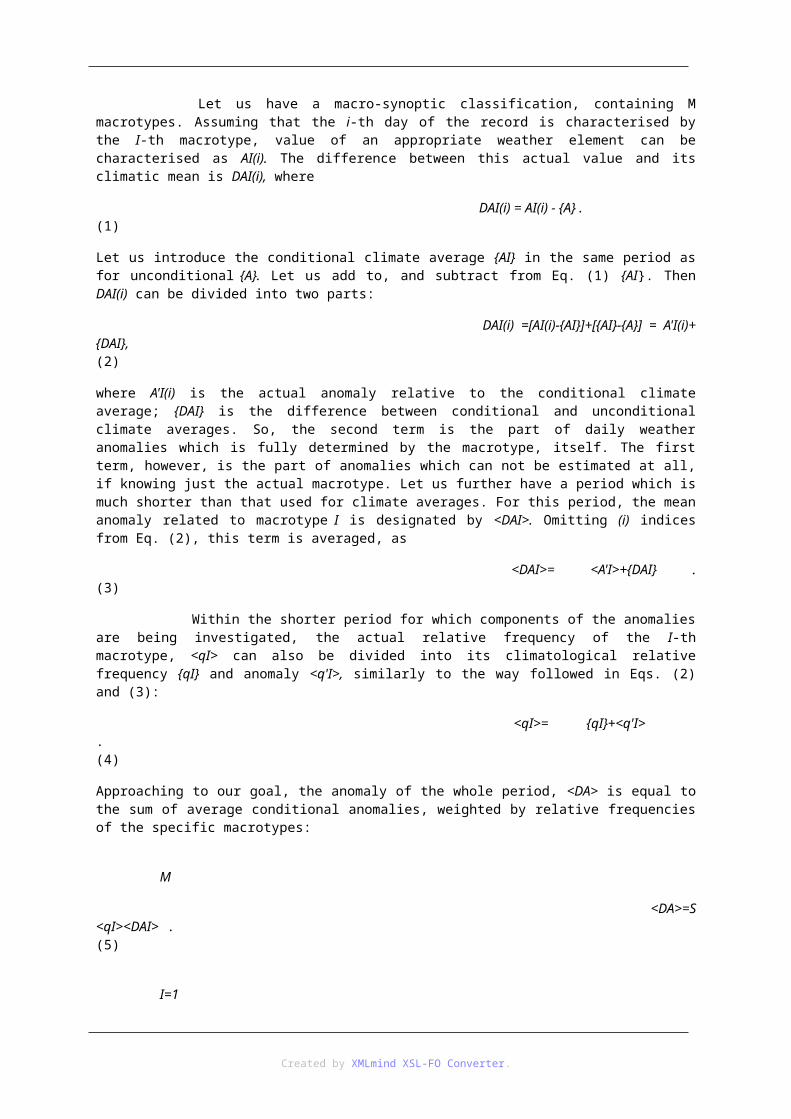
Let us have a macro-synoptic classification, containing M macrotypes. Assuming that the i-th day of the record is characterised by the I-th macrotype, value of an appropriate weather element can be characterised as AI(i). The difference between this actual value and its climatic mean is DAI(i), where

DAI(i) = AI(i) - {A} . (1)

Let us introduce the conditional climate average {AI} in the same period as for unconditional {A}. Let us add to, and subtract from Eq. (1) {AI}. Then DAI(i) can be divided into two parts:

DAI(i) =[AI(i)-{AI}]+[{AI}-{A}] = A'I(i)+{DAI}, (2)

where A'I(i) is the actual anomaly relative to the conditional climate average; {DAI} is the difference between conditional and unconditional climate averages. So, the second term is the part of daily weather anomalies which is fully determined by the macrotype, itself. The first term, however, is the part of anomalies which can not be estimated at all, if knowing just the actual macrotype. Let us further have a period which is much shorter than that used for climate averages. For this period, the mean anomaly related to macrotype I is designated by <DAI>. Omitting (i) indices from Eq. (2), this term is averaged, as

<DAI>= <A'I>+{DAI} . (3)

Within the shorter period for which components of the anomalies are being investigated, the actual relative frequency of the I-th macrotype, <qI> can also be divided into its climatological relative frequency {qI} and anomaly <q'I>, similarly to the way followed in Eqs. (2) and (3):

<qI>= {qI}+<q'I> . (4)

Approaching to our goal, the anomaly of the whole period, <DA> is equal to the sum of average conditional anomalies, weighted by relative frequencies of the specific macrotypes:

M

<DA>=S <qI><DAI> . (5)

I=1

Putting Eqs. (3) and (4) into Eq. (5), after elementary operations this expression can be written as

M M M M


<DA>= S{qI}{DAI}+S<q'I>{DAI}+S{qI}<A'I> +S<q'I><A'I> , (6)

I=1 I=1 I=1 I=1

where the first term is equal to zero, if only {qI} and {DAI} are calculated from the same reference period. The remaining three terms can be interpreted as follows:

S <q'I> { D AI} is the part of the <DA> anomaly due to anomalous frequency distribution of

macrotypes. This term of circulation origin is further referred as C.

S {qI} <A'I> is the part of anomaly, directly not influenced by frequencies of macrotypes.

This physical or non-circulation term, P, will be discussed in detail below.

S <q'I> <A'I> is the term ,M, due to mixed influence of both circulation and non-circulation

(physical) origin.

Let us mark <DA> as DY. Anomaly of a given period is equal to the sum of 3 terms:

DY = C + P + M . (7)

Information contained by frequency of macro-synoptic types, related to expected use of GCM-outputs, is included in term C and partly in term M. The physical term is determined by three processes: The first one is the initial large-scale anomaly, compared to the climatic mean pattern of the given macrotype, which is not great enough to select this pattern into a different class. This large-scale source of term P can appear parallel to climate variations and changes. The second source of term P can be originated in the local anomalies of the underlying surface (heat and moisture content) that, of course, might indirectly be influenced by the sequence of macrotypes within their fixed frequency distribution. Thirdly, term P may also contain the effects of scales not resolved by the horizontal grid-structure of the classification, or those connected to peculiarities of the actual vertical profiles, which are not represented by the sea-level pressure distribution, used by the classification.

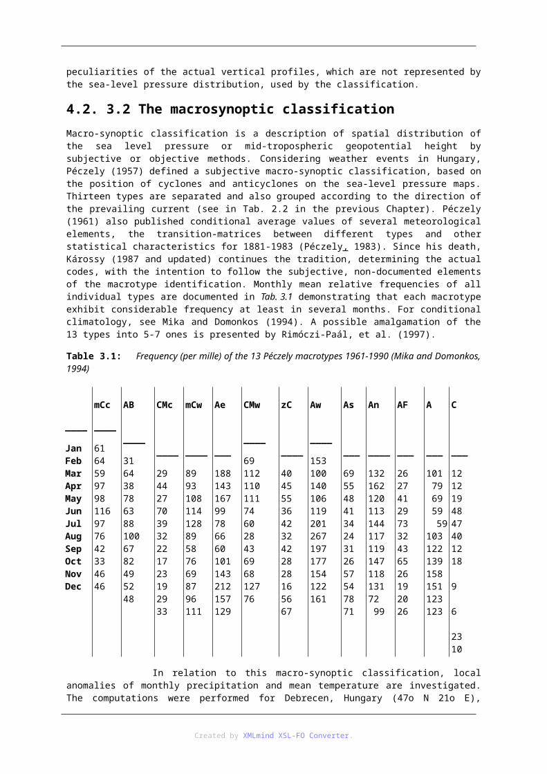
3.2. 3.2 The macrosynoptic classificationMacro-synoptic classification is a description of spatial distribution of the sea level pressure or mid-tropospheric geopotential height by subjective or objective methods. Considering weather events in Hungary, Péczely (1957) defined a subjective macro-synoptic classification, based on the position of cyclones and anticyclones on the sea-level pressure maps. Thirteen types are separated and also grouped according to the direction of the prevailing current (see in Tab. 2.2 in the previous Chapter). Péczely (1961) also published conditional average values of several meteorological elements, the transition-matrices between different types and other statistical characteristics for 1881-1983 (Péczely, 1983). Since his death, Károssy (1987 and updated) continues the tradition, determining the actual codes, with the intention to follow the subjective, non-documented elements of the macrotype identification. Monthly mean relative frequencies of all individual types are documented in Tab. 3.1 demonstrating that each macrotype exhibit considerable frequency at least in several months. For conditional climatology, see Mika and Domonkos (1994). A possible amalgamation of the 13 types into 5-7 ones is presented by Rimóczi-Paál, et al. (1997).

Table 3.1: Frequency (per mille) of the 13 Péczely macrotypes 1961-1990 (Mika and Domonkos, 1994)

____

Jan Feb Mar

mCc

____

61 64 59

AB

____

31 64

CMc

____

29 44

mCw

____

89 93 108

Ae

___

188 143

CMw

____

69 112 110 111

zC

____

40 45 55

Aw

____

153 100

As

___

69 55

An

____

132 162

AF

___

26 27 41 29

A

___

101 79

C

___

12 12


Apr May Jun Jul Aug Sep Oct Nov Dec

97 98 116 97 76 42 33 46 46

38 78 63 88 100 67 82 49 52 48

27 70 39 32 22 17 23 19 29 33

114 128 89 58 76 69 87 96 111

167 99 78 66 60 101 143 212 157 129

74 60 28 43 69 68 127 76

36 42 32 42 28 28 16 56 67

140 106 119 201 267 197 177 154 122 161

48 41 34 24 31 26 57 54 78 71

120 113 144 117 119 147 118 131 72 99

73 32 43 65 26 19 20 26

69 59 59 103 122 139 158 151 123 123

19 48 47 40 12 18 9 6 23 10

In relation to this macro-synoptic classification, local anomalies of monthly precipitation and mean temperature are investigated. The computations were performed for Debrecen, Hungary (47o N 21o E), located in a representative agricultural area, in each month between 1966 and 1995. Some seasonal or semi-annual results are also computed by averaging the monthly values, to exclude majority of the obvious seasonal effects. Termination of our computations with the year 1995 was forced by a change of instrumentation (automation of observations), that could lead to inhomogeneities of the local variables.

3.3. 3.3. Results of separation3.3.1. 3.3.1 Extreme and moderate anomalies

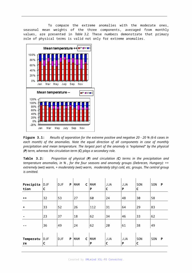
Results of separation for the extreme anomalies (++ and --) are presented in Figure 3.1. Note the equal direction of all components in case of monthly precipitation and mean temperature. Dominance of the P component is unequivocal mainly in case of the mean temperature. The largest part of the anomaly is "explained" by the physical (P) term, whereas the circulation term (C) plays a secondary role. Relative weights of circulation, physical and mixed components have no clear annual cycles.

To compare the extreme anomalies with the moderate ones, seasonal mean weights of the three components, averaged from monthly values, are presented in Table 3.2. These numbers demonstrate that primary role of physical terms is valid not only for extreme anomalies.

Figure 3.1: Results of separation for the extreme positive and negative 20 - 20 % (6-6 cases in each month) of


the anomalies. Note the equal direction of all components in case of monthly precipitation and mean temperature. The largest part of the anomaly is "explained" by the physical (P) term, whereas the circulation term (C) plays a secondary role.

Table 3.2: Proportion of physical (P) and circulation (C) terms in the precipitation and temperature anomalies, in % , for the four seasons and anomaly groups (Debrecen, Hungary): ++ extremely (wet) warm, + moderately (wet) warm, moderately (dry) cold, etc. groups. The central group is omitted.

Precipitation DJF C DJF P MAM C MAM P JJA C JJA P SON C SON P

++ 32 53 27 60 24 48 30 58

+ 33 52 26 112 31 64 29 83

- 23 37 18 62 34 46 33 62

-- 36 49 24 62 20 61 38 49

Temperature DJF C DJF P MAM C MAM P JJA C JJA P SON C SON P

++ 24 65 19 62 13 75 17 58

+ 16 71 17 69 25 46 28 53

- 22 82 20 67 11 74 13 71

-- 18 78 21 69 16 77 22 64

3.3.2. 3.3.2 Standard deviation

Standard deviation, computed for each component and for their sum, represents overall relation along the 30 years sample, as it is presented in Figure 3.2. Standard deviation of the sum is always much larger than that of the individual components. Dominating role of the physical term is also seen in these statistics, whereas circulation and mixed terms represent nearly identical contribution. Annual cycle of standard deviation for the sum (i.e. the total anomaly) is clearly reflected in the physical term and to much less extent in the other two terms.


Figure 3.2: Standard deviation of non-circulation physical (P), mixed (M) and circulation (C) terms and also of their sum (DY, the monthly anomaly) for precipitation and temperature in each month of the year.

3.3.3. 3.3.3 Long-term variations

Statistical downscaling of climate changes would mean application of relations, which are valid not only at the time scales of inter-annual variations, but also for the long-term changes. For this reason we computed five-year's averages of the monthly anomalies and also averaged them for the winter and summer half-years. Results of these operations are presented in Figure 3.3.


Figure 3.3: Contribution of the P, M and C terms to long-term variations of precipitation and temperature (five-years` moving averages). Note the big differences between the half-years in case of precipitation and the parallel run of the sum and the physical term in case of temperature. In the latter case, contribution of circulation and mixed terms are negligible.

Precipitation exhibit considerable differences in the two half-years considering the trends of the sum and the relative proportion of the terms. In the winter half-year fluctuations of the sum are not well reflected by any of the terms contributing to precipitation. In the summer half-year, the physical term largely contributes to long-term variations of the sum.

In case of temperature, C and M terms are not able to reflect a considerable part of the long-term behaviour of the sum, since the P term dominates the whole anomaly along the year. Moreover, this term exhibits almost identical run with the whole anomaly.

These results are not at all promising from the view-point of statistical downscaling based on frequency projections of diurnal circulation types..

3.3.4. 3.3.4 Correlation between the circulation term and the whole anomaly

Besides relative contributions to the average or standard deviation, it is worth analysing how the individual components correlate with their sum (i.e. with the monthly anomaly). Results of these computations are presented in Figure 3.4, from which one can realise the leading role of the physical term, again. Correlation of this term with the sum is always above the 95 % significance limit (0.35), except the inter-diurnal change in the majority of months. Correlation of the circulation term to the sum is also significant for both climate elements with the only exception of April in case of precipitation. This result is promising, considering feasibility of downscaling through frequency of circulation types: Even if low percentage of the anomaly is only captured by the circulation, high correlation of this component to the anomaly may lead to statistical additions that helps to better estimate the anomaly.


Figure 3.4: Correlation of physical (P), mixed (M) and circulation (C) terms to their sum (DY, i.e. the monthly anomaly) in each month of the year. The 95 % significance level (r = 0.35) is also indicated.

3.4. 3.4. DiscussionThe most important conclusion is the relatively minor role of the circulation term, except for low precipitation anomalies. It is impossible, however, to consider this circulation term as the maximum information contained by a series of macrotypes, because the succession of macrotypes is not taken into account by the separation. E.g. cool and wet westerlies at the beginning of the period, followed by warm and dry anticyclones could cause a much different monthly anomaly than the opposite case, although the frequency distribution would be the same.

Significant positive correlation of the circulation term with the whole anomaly is also promising in connection with the possibility of downscaling from the frequency of macrotypes, possibly in a more complex way. Such a way is demonstrated e.g. by Bartholy et al. (1995), who considered conditional autocorrelation under the given macrotype, as well. Another way to improve estimation capacity of diurnal circulation types is an inverse approach, where the classification is focused at a target element, not the large-scale patterns, themselves

3.5. 3.5 Mezo-scale eventsThe most dangerous extreme weather events are caused or atz least supported by convection. This strong and arranged vertical motion leads to adiabatic heating of ascending air particles. In consequence their temperature is decreasing by 1 Celsius per every 100 m of elevation.

First we present a series of a devastating supercell (Fig. 3.5) and further comprehend the possible consequences of the inherent atmospheric process, the convection.


Fig. 3.5: Life-cycle of a super-cell in time sequence. Photo: Attila Gazdag and Endre Harc on July, 14, 2009 in Letenye (Zala county, Hungary) downloaded from http://blog.xfree.hu/myblog.tvn?n=bobeacs&pid=32101

Vertical motion, called convection is the key to the most dangerousatmospheric phenomena. Fig. 3.6 indicates those events which are generally formed by convection.

Later in Fig 3.7 the pentagonal structure of the Hungarian Lightning Detection network is presented which is important indicator of stating or intensifying electronic activity int he developing vertical cloudiness.


Another zse of this tool is to provide objective validation concerning the question if lightning really did hit a built object, or not.

Fig. 3.6: Mezos-scale objects caused by convection in their increasing sequence of horizontal size and intensity. (In field 6. squall line means vertical istability ordered linearly. Courtesy to Dr. Ákos Horváth for providing this Figure.)

Fig. 3.7: The Hungarian Lightning Detection Network


3.6. 3.6 Classification of icing and hailstorm intensities

In the followings, two dangerous event’s classification is provided, based on their intensity and caused potential harm. Table 3.3 concerns icing, whereas Table 3.4 lists intensity scaling for hailstorms. Both tables have rather extreme maxima, frequency of which events is rather law.

Table 3.3: Intensity scaling for icing on the structures (Burt, 2007)

Table 3.3: Intensity scaling for hailstorms (Burt, 2007)


3.7. 3.7 The European weather warning system

In the first decade of our 21th century several European Meteorological Services started to cooperate in storm warning by later creation of the Meteoalarm cooperation. An example of the maps they provide via Internet is seen in Fig. 3.8 indicating the extremities the warning system deals with. The colouring i.e. the levels of warning are presented in Fig. 3.9 according to the French MetService. (As the vulnerability and exposure is different in the various regions, some differences also exist in understanding the various levels (colours). It is important however, that the extraordinary warning (red colour) should only be applied rather rarely.

Fig. 3.8: The Meteoralarm warning situation on 07.03. 2007.

Fig. 3.8: Threshold for each weather warning parameter (colour).

See also ANIM_3_1 and ANIM_3_2, presenting the tragical August 20, 2006 in radar images, and a series of micro-regional warning in Hungary from another day, in the moving images.


FILM_3_1_thounderstorm_in_visible.avi and FILM_3_2_ thounderstorm_in infrared.avi both document the development of a thounderstom cell by using visible and infrared channels of METEOSAT satellites. Both films represent May 20, 2008.

4. 3. Effects of mezo-scalesSophisticated efforts to use GCM-outputs for regional climate scenario construction can be sorted into two groups. In both approaches, however, accuracy of the large-scale flow generated in the GCM is crucial. The first possibility is a one-way coupling of a limited-area model into the original sequence of GCM-fields. At present this approach is beyond the possibility of many research institutions due to its high demand in computer capacity and initialisation efforts.

The second way is to combine larger scale averages, or pattern components of the model-generated fields with empirical relationships, learned on measured data sets, between the large-scale characteristics and regional anomalies. In terminology of forecasters, this combination of model generated fields with empirical connections is a "perfect prognosis" approach. That is, a statistical model is developed between dynamic and prognostic quantities in the presently observed atmosphere, and it is applied to the simulated (future) atmosphere with no respect to the possible systematic deviation of the projected circulation patterns from the really occurring ones.

To test this approach, a method is introduced to calculate the relative contribution of macro-circulation anomalies, expressed by frequency distribution among finite number of classes, to the climate anomalies. After describing the method (Section 3.1), the applied objective macro-synoptic classification (Section 3.2) is introduced. Results are presented for monthly anomalies of five weather characteristics: precipitation, mean, maximum and minimum temperatures; and inter-diurnal change of mean temperature. The results are structured according to the presented statistical characteristics. Section 3.3.1 demonstrates behaviour of moderate and extreme anomalies. Section 3.3.2 presents the standard deviations and Section 3.3.3 displays contribution of the terms to the long-term tendencies. Finally, Section 3.3.4 analyses the correlation between the components and their sum (i.e. the anomaly). Section 3.4 contributes to discussion on applicability of the macro-circulation types in statistical downscaling. Mezos-scale events, mostly created by convection are briefly presented in Section 3.5. Classification of two significant extremities, icing and hailstorms are displayed in Section 3.6. Finally, European weather warning systems is presented in Section 3.7.

4.1. 3.1 The method of separationThe aim of this method is to quantify, what part of climate anomalies can be directly attributed to the anomalous frequency distribution of macro-synoptic types in the period for which the anomaly is formed. The following elementary operations will conclude at a separation of the anomalies, where this term is one of their three, non-zero components (Mika, 1993).

Let us have a macro-synoptic classification, containing M macrotypes. Assuming that the i-th day of the record is characterised by the I-th macrotype, value of an appropriate weather element can be characterised as AI(i). The difference between this actual value and its climatic mean is DAI(i), where

DAI(i) = AI(i) - {A} . (1)

Let us introduce the conditional climate average {AI} in the same period as for unconditional {A}. Let us add to, and subtract from Eq. (1) {AI}. Then DAI(i) can be divided into two parts:

DAI(i) =[AI(i)-{AI}]+[{AI}-{A}] = A'I(i)+{DAI}, (2)

where A'I(i) is the actual anomaly relative to the conditional climate average; {DAI} is the difference between conditional and unconditional climate averages. So, the second term is the part of daily weather anomalies which is fully determined by the macrotype, itself. The first term, however, is the part of anomalies which can not be estimated at all, if knowing just the actual macrotype. Let us further have a period which is much shorter than that used for climate averages. For this period, the mean anomaly related to macrotype I is designated by <DAI>. Omitting (i) indices from Eq. (2), this term is averaged, as


<DAI>= <A'I>+{DAI} . (3)

Within the shorter period for which components of the anomalies are being investigated, the actual relative frequency of the I-th macrotype, <qI> can also be divided into its climatological relative frequency {qI} and anomaly <q'I>, similarly to the way followed in Eqs. (2) and (3):

<qI>= {qI}+<q'I> . (4)

Approaching to our goal, the anomaly of the whole period, <DA> is equal to the sum of average conditional anomalies, weighted by relative frequencies of the specific macrotypes:

M

<DA>=S <qI><DAI> . (5)

I=1

Putting Eqs. (3) and (4) into Eq. (5), after elementary operations this expression can be written as

M M M M

<DA>= S{qI}{DAI}+S<q'I>{DAI}+S{qI}<A'I> +S<q'I><A'I> , (6)

I=1 I=1 I=1 I=1

where the first term is equal to zero, if only {qI} and {DAI} are calculated from the same reference period. The remaining three terms can be interpreted as follows:

S <q'I> { D AI} is the part of the <DA> anomaly due to anomalous frequency distribution of

macrotypes. This term of circulation origin is further referred as C.

S {qI} <A'I> is the part of anomaly, directly not influenced by frequencies of macrotypes.

This physical or non-circulation term, P, will be discussed in detail below.

S <q'I> <A'I> is the term ,M, due to mixed influence of both circulation and non-circulation

(physical) origin.

Let us mark <DA> as DY. Anomaly of a given period is equal to the sum of 3 terms:

DY = C + P + M . (7)

Information contained by frequency of macro-synoptic types, related to expected use of GCM-outputs, is included in term C and partly in term M. The physical term is determined by three processes: The first one is the initial large-scale anomaly, compared to the climatic mean pattern of the given macrotype, which is not great enough to select this pattern into a different class. This large-scale source of term P can appear parallel to climate variations and changes. The second source of term P can be originated in the local anomalies of the underlying surface (heat and moisture content) that, of course, might indirectly be influenced by the sequence of macrotypes within their fixed frequency distribution. Thirdly, term P may also contain the effects of scales not resolved by the horizontal grid-structure of the classification, or those connected to peculiarities of the actual vertical profiles, which are not represented by the sea-level pressure distribution, used by the classification.

4.2. 3.2 The macrosynoptic classification


Macro-synoptic classification is a description of spatial distribution of the sea level pressure or mid-tropospheric geopotential height by subjective or objective methods. Considering weather events in Hungary, Péczely (1957) defined a subjective macro-synoptic classification, based on the position of cyclones and anticyclones on the sea-level pressure maps. Thirteen types are separated and also grouped according to the direction of the prevailing current (see in Tab. 2.2 in the previous Chapter). Péczely (1961) also published conditional average values of several meteorological elements, the transition-matrices between different types and other statistical characteristics for 1881-1983 (Péczely, 1983). Since his death, Károssy (1987 and updated) continues the tradition, determining the actual codes, with the intention to follow the subjective, non-documented elements of the macrotype identification. Monthly mean relative frequencies of all individual types are documented in Tab. 3.1 demonstrating that each macrotype exhibit considerable frequency at least in several months. For conditional climatology, see Mika and Domonkos (1994). A possible amalgamation of the 13 types into 5-7 ones is presented by Rimóczi-Paál, et al. (1997).

Table 3.1: Frequency (per mille) of the 13 Péczely macrotypes 1961-1990 (Mika and Domonkos, 1994)

____

Jan Feb Mar Apr May Jun Jul Aug Sep Oct Nov Dec

mCc

____

61 64 59 97 98 116 97 76 42 33 46 46

AB

____

31 64 38 78 63 88 100 67 82 49 52 48

CMc

____

29 44 27 70 39 32 22 17 23 19 29 33

mCw

____

89 93 108 114 128 89 58 76 69 87 96 111

Ae

___

188 143 167 99 78 66 60 101 143 212 157 129

CMw

____

69 112 110 111 74 60 28 43 69 68 127 76

zC

____

40 45 55 36 42 32 42 28 28 16 56 67

Aw

____

153 100 140 106 119 201 267 197 177 154 122 161

As

___

69 55 48 41 34 24 31 26 57 54 78 71

An

____

132 162 120 113 144 117 119 147 118 131 72 99

AF

___

26 27 41 29 73 32 43 65 26 19 20 26

A

___

101 79 69 59 59 103 122 139 158 151 123 123

C

___

12 12 19 48 47 40 12 18 9 6 23 10

In relation to this macro-synoptic classification, local anomalies of monthly precipitation and mean temperature are investigated. The computations were performed for Debrecen, Hungary (47o N 21o E), located in a representative agricultural area, in each month between 1966 and 1995. Some seasonal or semi-annual results are also computed by averaging the monthly values, to exclude majority of the obvious seasonal effects. Termination of our computations with the year 1995 was forced by a change of instrumentation (automation of observations), that could lead to inhomogeneities of the local variables.

4.3. 3.3. Results of separation4.3.1. 3.3.1 Extreme and moderate anomalies

Results of separation for the extreme anomalies (++ and --) are presented in Figure 3.1. Note the equal direction of all components in case of monthly precipitation and mean temperature. Dominance of the P component is unequivocal mainly in case of the mean temperature. The largest part of the anomaly is "explained" by the physical (P) term, whereas the circulation term (C) plays a secondary role. Relative weights of circulation, physical and mixed components have no clear annual cycles.

To compare the extreme anomalies with the moderate ones, seasonal mean weights of the three components, averaged from monthly values, are presented in Table 3.2. These numbers demonstrate that primary role of physical terms is valid not only for extreme anomalies.


Figure 3.1: Results of separation for the extreme positive and negative 20 - 20 % (6-6 cases in each month) of the anomalies. Note the equal direction of all components in case of monthly precipitation and mean temperature. The largest part of the anomaly is "explained" by the physical (P) term, whereas the circulation term (C) plays a secondary role.

Table 3.2: Proportion of physical (P) and circulation (C) terms in the precipitation and temperature anomalies, in % , for the four seasons and anomaly groups (Debrecen, Hungary): ++ extremely (wet) warm, + moderately (wet) warm, moderately (dry) cold, etc. groups. The central group is omitted.

Precipitation DJF C DJF P MAM C MAM P JJA C JJA P SON C SON P

++ 32 53 27 60 24 48 30 58

+ 33 52 26 112 31 64 29 83

- 23 37 18 62 34 46 33 62

-- 36 49 24 62 20 61 38 49

Temperature DJF C DJF P MAM C MAM P JJA C JJA P SON C SON P

++ 24 65 19 62 13 75 17 58

+ 16 71 17 69 25 46 28 53

- 22 82 20 67 11 74 13 71

-- 18 78 21 69 16 77 22 64

4.3.2. 3.3.2 Standard deviation


Standard deviation, computed for each component and for their sum, represents overall relation along the 30 years sample, as it is presented in Figure 3.2. Standard deviation of the sum is always much larger than that of the individual components. Dominating role of the physical term is also seen in these statistics, whereas circulation and mixed terms represent nearly identical contribution. Annual cycle of standard deviation for the sum (i.e. the total anomaly) is clearly reflected in the physical term and to much less extent in the other two terms.

Figure 3.2: Standard deviation of non-circulation physical (P), mixed (M) and circulation (C) terms and also of their sum (DY, the monthly anomaly) for precipitation and temperature in each month of the year.

4.3.3. 3.3.3 Long-term variations

Statistical downscaling of climate changes would mean application of relations, which are valid not only at the time scales of inter-annual variations, but also for the long-term changes. For this reason we computed five-year's averages of the monthly anomalies and also averaged them for the winter and summer half-years. Results of these operations are presented in Figure 3.3.


Figure 3.3: Contribution of the P, M and C terms to long-term variations of precipitation and temperature (five-years` moving averages). Note the big differences between the half-years in case of precipitation and the parallel run of the sum and the physical term in case of temperature. In the latter case, contribution of circulation and mixed terms are negligible.

Precipitation exhibit considerable differences in the two half-years considering the trends of the sum and the relative proportion of the terms. In the winter half-year fluctuations of the sum are not well reflected by any of the terms contributing to precipitation. In the summer half-year, the physical term largely contributes to long-term variations of the sum.

In case of temperature, C and M terms are not able to reflect a considerable part of the long-term behaviour of the sum, since the P term dominates the whole anomaly along the year. Moreover, this term exhibits almost identical run with the whole anomaly.

These results are not at all promising from the view-point of statistical downscaling based on frequency projections of diurnal circulation types..


4.3.4. 3.3.4 Correlation between the circulation term and the whole anomaly

Besides relative contributions to the average or standard deviation, it is worth analysing how the individual components correlate with their sum (i.e. with the monthly anomaly). Results of these computations are presented in Figure 3.4, from which one can realise the leading role of the physical term, again. Correlation of this term with the sum is always above the 95 % significance limit (0.35), except the inter-diurnal change in the majority of months. Correlation of the circulation term to the sum is also significant for both climate elements with the only exception of April in case of precipitation. This result is promising, considering feasibility of downscaling through frequency of circulation types: Even if low percentage of the anomaly is only captured by the circulation, high correlation of this component to the anomaly may lead to statistical additions that helps to better estimate the anomaly.

Figure 3.4: Correlation of physical (P), mixed (M) and circulation (C) terms to their sum (DY, i.e. the monthly anomaly) in each month of the year. The 95 % significance level (r = 0.35) is also indicated.

4.3.5. 3.4. Discussion

The most important conclusion is the relatively minor role of the circulation term, except for low precipitation anomalies. It is impossible, however, to consider this circulation term as the maximum information contained by a series of macrotypes, because the succession of macrotypes is not taken into account by the separation. E.g. cool and wet westerlies at the beginning of the period, followed by warm and dry anticyclones could cause a much different monthly anomaly than the opposite case, although the frequency distribution would be the same.

Significant positive correlation of the circulation term with the whole anomaly is also promising in connection with the possibility of downscaling from the frequency of macrotypes, possibly in a more complex way. Such a way is demonstrated e.g. by Bartholy et al. (1995), who considered conditional autocorrelation under the given macrotype, as well. Another way to improve estimation capacity of diurnal circulation types is an inverse approach, where the classification is focused at a target element, not the large-scale patterns, themselves

4.4. 3.5 Mezo-scale events


The most dangerous extreme weather events are caused or atz least supported by convection. This strong and arranged vertical motion leads to adiabatic heating of ascending air particles. In consequence their temperature is decreasing by 1 Celsius per every 100 m of elevation.

First we present a series of a devastating supercell (Fig. 3.5) and further comprehend the possible consequences of the inherent atmospheric process, the convection.

Fig. 3.5: Life-cycle of a super-cell in time sequence. Photo: Attila Gazdag and Endre Harc on July, 14, 2009 in


Letenye (Zala county, Hungary) downloaded from http://blog.xfree.hu/myblog.tvn?n=bobeacs&pid=32101

Vertical motion, called convection is the key to the most dangerousatmospheric phenomena. Fig. 3.6 indicates those events which are generally formed by convection.

Later in Fig 3.7 the pentagonal structure of the Hungarian Lightning Detection network is presented which is important indicator of stating or intensifying electronic activity int he developing vertical cloudiness. Another zse of this tool is to provide objective validation concerning the question if lightning really did hit a built object, or not.

Fig. 3.6: Mezos-scale objects caused by convection in their increasing sequence of horizontal size and intensity. (In field 6. squall line means vertical istability ordered linearly. Courtesy to Dr. Ákos Horváth for providing this Figure.)


Fig. 3.7: The Hungarian Lightning Detection Network

4.5. 3.6 Classification of icing and hailstorm intensities

In the followings, two dangerous event’s classification is provided, based on their intensity and caused potential harm. Table 3.3 concerns icing, whereas Table 3.4 lists intensity scaling for hailstorms. Both tables have rather extreme maxima, frequency of which events is rather law.

Table 3.3: Intensity scaling for icing on the structures (Burt, 2007)


Table 3.3: Intensity scaling for hailstorms (Burt, 2007)

4.6. 3.7 The European weather warning system

In the first decade of our 21th century several European Meteorological Services started to cooperate in storm warning by later creation of the Meteoalarm cooperation. An example of the maps they provide via Internet is seen in Fig. 3.8 indicating the extremities the warning system deals with. The colouring i.e. the levels of warning are presented in Fig. 3.9 according to the French MetService. (As the vulnerability and exposure is different in the various regions, some differences also exist in understanding the various levels (colours). It is important however, that the extraordinary warning (red colour) should only be applied rather rarely.

Fig. 3.8: The Meteoralarm warning situation on 07.03. 2007.


Fig. 3.8: Threshold for each weather warning parameter (colour).

See also ANIM_3_1 and ANIM_3_2, presenting the tragical August 20, 2006 in radar images, and a series of micro-regional warning in Hungary from another day, in the moving images.

FILM_3_1_thounderstorm_in_visible.avi and FILM_3_2_ thounderstorm_in infrared.avi both document the development of a thounderstom cell by using visible and infrared channels of METEOSAT satellites. Both films represent May 20, 2008.

5. 4. Zonality and continentality

Terms zonality and continentality are used in geography to characterise spatial features of the present climate. Since we have global climate models, one can judge objectively whether these features are direct consequences of those physical differences which are often used when these concepts are introduced. This is the aim of our paper, as well. Narrow zonal and meridional belts are defined and the recent GCM outputs, adjusted by the MAGICC SCENGEN software (Wigley, 2008) will be analysed, besides the present climate, which is applied by the same software from the ERA-40 (Uppala et al., 2005).

5.1. 4.1 Global climate modelsThe model simulations are based on the A1B SRES scenario (IPCC, 2007). The forecasted and control periods are 2071-2100 vs. 1980-1999. The main features of the models are listed in Table 1. Majority of the models are new compared to the previous IPCC Report. In some cases, similar models of the same institute are used with differences in the resolution, or in parameterization of one single process.

Table 4.1. Characteristics of the 20 OAGCMs (IPCC 2007 WG-I, Ch. 8, 597-599) results of which are averaged. The order of information: host-institution, upper boundary (top), vertical and horizontal resolution in atmosphere (A) and ocean (O). These models are also used in the MAGICC/SCENGEN diagnostic model, except the GISS-AOM (upper right field of the table).

GISS-EH, 2004: NASA Goddard Institute for Space Studies, USA, top = 0.1 hPa, L20

A: 4° x 5° O: 2° x 2° L16

GISS-ER, 2004: NASA Goddard Institute for Space Studies, USA, top = 0.1 hPa L20

A: 4° x 5° O:4° x 5° L13


GFDL-CM2.0, 2005: NOAA/Geophysical Fluid Dyn. Lab., USAtop = 3 hPa L24,

A: 2.0° x 2.5° O: 0.3°–1.0° x 1.0°

GFDL-CM2.1, 2005 NOAA/Geophysical Fluid Dyn. Lab., USA, =GFDL-CM2.0 with semi-Lagrangian atmospheric transport

CGCM3.1(T47), 2005: Canad. Centre for Clim. Mod. Anal., Canada, top =1 hPa, L31

A: T47 (~2.8° x 2.8°) O: 1.9° x 1.9° L29

CGCM3.1(T63), 2005: Canad. Centre for Clim. Mod. Anal., Canada, top =1 hPa, L31

A: T63 (~1.9° x 1.9°), O: 0.9° x 1.4° L29

MIROC3.2(hires), 2004: U.Tokyo; Nat. Ins. Env. Stud.; JAMSTEC,Japan top=40 km,L56

A: T106 (~1.1° x 1.1°) O: 0.2° x 0.3° L47

MIROC3.2(medres),2004: U.Tokyo; Nat. Ins. Env. Stud.; JAMSTEC,Japan top = 30 km L20

A: T42 (~2.8°x2.8°) O: 0.5°–1.4°x1.4° L43

UKMO-HadCM3, 1997: Hadley Centre / Meteorol. Office, UK top =5 hPa, L19

A: 2.5° x 3.75° O: 1.25° x 1.25° L20

UKMO-HadGEM1, 2004: Hadley Centre/ Meteorol. Office, UK top = 39.2 km, L38

A: ~1.3° x 1.9° O: 0.3°–1.0° x 1.0° L40

CCSM3, 2005 : National Center for Atmosph. Res., USA, top = 2.2 hPa, L26

A: T85 (1.4°x1.4°), O: 0.3°–1°x1°, L40

CNRM-CM3, 2004: Météo-France/Centre Nat. Rech. Mét.. France, top=0.05 hPa L45, A: T63 (~1.9° x 1.9°) O: 0.5°–2° x 2° L31

CSIRO-MK3.0, 2001: Comm. Sci. Industr. Res. Org., Australia,top = 4.5 hPa, L18

A: T63 (~1.9° x 1.9°) O: 0.8° x 1.9° L31

ECHAM5/MPI-OM, 2005: Max Planck Inst. f. Meteor., Germany, top=10 hPa, L31 A: T63 (~1.9° x 1.9°), O: 1.5° x 1.5° L40

ECHO-G, 1999 Meteor. Inst. Univ. Bonn, FRG, Met. Res. Inst. Korea,top=10 hPa L19

A: T30 (~3.9°x3.9°) O: 0.5°–2.8°x2.8° L20

FGOALS-g1.0, 2004: Nat. Key Lab. /Inst. Atmos. Phys., China, top = 2.2 hPa, L26

A: T42 (~2.8° x 2.8°) O: 1.0° x 1.0° L16

INM-CM3.0, 2004: Institute for Numerical Mathematics, Russia top = 10 hPa, L21

A: 4° x 5° O: 2° x 2.5° L33

IPSL-CM4, 2005: Institut Pierre Simon Laplace, France top = 4 hPa, L19

A: 2.5° x 3.75° O:2° x 2° L31

MRI-CGCM2, 2003: Meteorological Res. Institute, Japan top = 0.4 hPa L30

A: T42 (~2.8°x2.8°) O: 0.5°–2.0°x2.5° L23

PCM, 1998: National Center for Atmosph. Research, USA top = 2.2 hPa L26

A: T42 (~2.8°x2.8°) O:0.5°–0.7°x1.1° L40

Having introduced the global models, the zonal and meridional features of climate wil be listed including the model biases and the appearance of these key geographical terms in the fields of changes. The section is terminated by description of the term, weathering

5.2. 4.2 The MAGIC/SCENGEN diagnostic modelIn order to generate climate scenario on local and regional scales, a relatively simple tool, namely, the MAGICC/SCENGEN 5.3 software package (Wigley et al., 2008) was applied. All these newest GCMs were evaluated by the AR4 (IPCC, 2007). The global section of the package, the MAGICC, is based on an up-welling diffusion energy balance model calibrated by global sensitivity of the GCMs outputs. For a selected region, the large number of GCM output fields may reduce the existing uncertainty of climate prediction. In this section 20 GCMs treated by the package are considered.


Local climate change is strongly influenced by local features such as mountains, which are not well represented in global climate models. Yet, despite these deficiencies, GCMs play an important role in regional climate research. In the followings the above model outputs are averaged and synchronised by the MAGICC/SCENGEN 5.3 diagnostic software tool. Temperature, precipitation and sea-level pressure data are analysed. The SCENGEN applies linear scaling from the output fields from each model.

5.3. 4.3 The selected beltsThe investigated zonal belt is set between the 45-50°N latitudes. It has been chosen, as it contains the homeland of the authors and a wide variety of lowlands and mountains, warm and cold sectors of oceans, what makes the comparative research more conducive. In favour of better comparability and transparency, 10 sample area has been defined within this temperate belt. Every entitled area (Figure 4.1) contains 10-10 rectangles of the 2.5o

long x 2.5o lat fields, in which data data, the errors and the changes are given. The meridional belt is just 2.5 deg wide and spreads from the North Pole to the South Pole along the 18.75E meridian, and continues along the 161.75W meridian.


FIG 4.1: Map of the investigated zonal and meridional belts. In the zonal belt, between 45 th and 50th latitudes, the abbreviations are as follows. Pa1 – Pa2: the Pacific, cold resp. warm current; Am1 – Am2: North-America: mountains resp. plains and lakes; At1 – At2: the Atlantic: cold resp. warm current; Eu1 – Eu2: Europe: mountains (Alps and Carpathians) resp. plains; As1 – As2: Asia: table-land, mountains resp. mountains.

5.4. 4.4 Zonality and continentality in the present climateThree aspects of temperature, precipitation and sea-level pressure fields are investigated concerning zonality and continentality. All of them are reduced to the above specified zonal and meridional belts. These aspects are (i) the present observed fields and (ii) the bias error of the simulated fields derived from the 20 GCMs and adjusted by the MAGICC/SCENGEN software tool, and finally, the changes in the elements between the foreseen 2030-2049 period compared to the 1980-1999 reference period. The first two aspects are seen in Figs. 4.2-4.4 in respect to zonality, and Figs 4.5-4.7 to continentality.

For the temperature (Fig. 4.2), besides the obvious zonality of the seasonal mean temperature in both extreme seasons, one can establish slight overestimation in the tropical and temperate latitudes with strong underestimation in Polar regions of both hemispheres. This underestimation is stronger in the belt crossing mainly continental regions (along 18.75 E) than in the one, spreading over the oceans (along 161.75 W).

For precipitation, even the observed mean values are interesting along the two different belts (Fig 4.3.). Not only the oceanic belt is characterised by much higher values in both seasons in many latitudes, but shapes of the zonal profiles are different in both seasons.

The errors are mainly over-estimations except the tropical latitudes with a few critical relative overestimations at some latitudes where the observed values are generally low. The dependence of the bias on the latitudes is rather different in the mainly oceanic vs. the mainly continental belts, spreading between the Poles.

WINTER SUMMER


Fig. 4.2: Observed mean values (upper graphs) and simulation bias (lower) of temperature (oC) in winter (left) and in summer (right) in the meridional belt representing zonality.

WINTER SUMMER

Fig. 4.3. Observed values (mm/d: upper) and simulation bias (%: lower) of precipitation in winter (left) and in summer (right) in the meridional belt representing zonality.

For the observed values of sea-level pressure we can see considerable phase shifts between the two meridians indicating big differences between continental and oceanic areas of both hemispheres. The latitudinal dependence of the sea-level pressure is also clearly seen in the upper graphs of Fig. 4.4. For the zonal sections (Fig, 4.5) one may see clear differences indicating the higher pressure over continents in winter and over the oceans in summer. The bias errors along the meridional section are high again in the Polar regions where the models mainly overestimate the seasonal mean pressure of these regions. For the zonal belts, in winter the Eurasian continent is under-estimated with overestimations of some oceans. In summer the bias errors are much smaller.

WINTER SUMMER


Fig. 4.4: Observed values (upper graphs) and simulation bias (lower) of sea-level pressure (hPa) in winter (left) and in summer (right) in the meridional belt representing zonality.

WINTER SUMMER

Fig. 4.5. Observed values (upper graphs) and simulation bias (lower) of sea-level pressure (hPa) in winter (left) and in summer (right) in the zonal belt representing continentality.

The continentality is clearly seen in the latitudinal belts (Fig. 4.6). High temperature is seen in the eastern borders of oceans between the continents in winter, but in summer the eastern parts of the continents have relative maxima. Precipitation indicates strong differences between the continental and oceanic areas of the given belt. The models mainly underestimate the temperature with deviations also related to the nature of the surface. In winter the models strongly overestimate precipitation in some dry regions. In summer the estimations are better and not clearly continent/ocean dependent.


WINTER SUMMER

Fig. 4.6: Observed values (upper graphs) and simulation bias (lower) of temperature ( oC) in winter (left) and in summer (right) in the zonal belt representingcontinentality.

WINTER SUMMER

Fig. 4.7: Observed values (mm/d: upper) and simulation bias (%: lower) of precipitation in winter (left) and in summer (right) in the zonal belt representing continentality.

5.5. 4.5 Zonality and continentality in the projected changes

Changes of climate variables are derived by (large-scale) physics of the climate models. Hence, one may expect occurrence of zonality and continentality in the changes, as well.


WINTER SUMMER

Fig. 4.8: Projected changes of temperature (oC) in the meridional belt representing zonality between 2030-2049 and 1980-1999 according to GHG-only, A1B scenario.

WINTER SUMMER

Fig. 4.9. Projected changes of temperature (oC) in the zonal belt representing continent-tality between 2030-2049 and 1980-1999 according to GHG-only, A1B scenario.

The stronger changes of temperature in winter indicate no unequivocal differences in winter but much weaker changes in summer over the ocean-based section (Fig. 4.8). Along the latitudinal belts (Fig. 4.9) the warming is generally stronger over the continents. Forprecipitation (Fig. 4.10) the changes are mainly positive along the oceanic meridional belt in winter. Along the continental one, the changes are different. In summer the situation is similar with rather hectic differences along the continental meridional belt.

WINTER SUMMER

Fig. 4.10: Projected changes of precipitation (%) in the zonal belt representing continent-tality between 2030-2049 and 1980-1999 according to GHG-only, A1B scenario.


WINTER SUMMER

Fig. 4.11: Projected changes of precipitation (%) in the meridional belt representing zonality between 2030-2049 and 1980-1999 according to GHG-only, A1B scenario.

WINTER SUMMER

Fig. 4.12. Projected changes of sea-level pressure (hPa) in the zonal belt representing con-tinentality between 2030-2049 and 1980-1999 according to GHG-only, A1B scenario.

WINTER SUMMER

Fig. 13. Projected changes of sea-level pressure (hPa) in the meridional belt represent-ting zonality between 2030-2049 and 1980-1999 according to GHG-only, A1B scenario.

Along the zonal belt, there are moderate positive changes of precipitation almost everywhere with one peak towards Asia (Fig. 4.11). In summer the changes are negative in majority of the circle with no unequivocal continent vs. ocean differences. Sea-level pressure changes are in anti-phase along the oceanic vs. continental meridian in winter with compensation of the slight decrease along the continent by the oceanic meridian in summer (Fig. 4.12). In the zonal belt, longitudinal dependence of pressure changes is seen in both seasons, with no simple statements on continentality (Fig 4.13).

5.6. 4.6 Weathering: a complex effect of climate


Weathering is the process of disintegration of rock from physical, chemical, and biological stresses. I.e. this is one of the processes in our Planet which can well be explained in each of the four natural sciences, physics, chemistry, biology and geography. Weathering is influenced by temperature and moisture (climate). As rock disintegrates, it becomes more susceptible to further physical, chemical, and biological effects due to the increase in exposed surface area. During weathering, minerals that were once bound in the rock are released.

The degree of weathering that occurs depends upon the resistance to weathering of the minerals in the rock, as well as the degree of the physical, chemical, and biological stresses. A rule of thumb is that minerals in rocks that are formed under high temperature and pressure are less resistant to weathering, while minerals formed at low temperature and pressure are more resistant to weathering. Weatheringis usually confined to the top few meters of geologic material, because physical, chemical, and biological stresses generally decrease with depth. Weathering of rocks occurs in place, but the disintegrated weathering products can be carried by water, wind, or gravity to another location (i.e. erosion or mass-losing). This figure is a fairly good one for both physics, chemistry as well, as geography teachers to emphasize corresponding aspects of their topic.

Figure 4.14 indicates how temperature affects weathering in our present climate. javascript:void(window.open('/croptechnology2005/UserFiles/Image/Martha/Principles%20Lesson%202%20/Annual-Rain-Temp(1).gif','','resizable=yes,location=no,menubar=no,scrollbars=yes,status=no,toolbar=no,fullscreen=no,dependent=no'))

Figure 4.14: . Influence of the interaction of temperature and rainfall on processes of physical and chemical weathering. As annual rainfall and temperature increase, chemical weathering dominates over physical


weathering. On the contrary, notice that as the temperature lowers, physical weathering begins to dominate over chemical weathering. Image courtesy of University of Nebraska–Lincoln,2005. http://plantandsoil.unl.edu/crop technology2005/soil_sci/ ?what=topicsD& informationModuleId=1124303183&topicOrder=2&max=7&min=0&

6. 5.On correlation of maize and wheat yield with vegetation indexThe aim of the Section is to quantify statistical relations between the Normalized Differential Vegetation Index (NDVI), derived from NOAA/AVHRR multi-channel irradiance, and yield of wheat and maize commonly covering 23.5 % of Hungary. The 14 years period, 1985-1998 is used, reserving the later vegetation seasons for independent validation, in the future. The yield reporting units are the 19 administrative counties, characterized by 50-90 km of linear measure and diverse vegetation. Cluster analysis of the yield series is performed to identify possible outliers, but there are no qualitatively separating outliers found among the 14 years and 19 counties for the investigated plants. The same procedure is performed for the average proportion of land-use types and for the NDVI series with the aim of finding coherent groups of counties to unify them into larger, cumulative samples. However, these analyses did not yield the necessary similarities, hence, no further spatial integration was performed. The applied NDVI series are filtered against possible remained atmospheric disturbances, whereas the yield data are standardized against the, actually decreasing, linear trends. The relationships between weekly composite NDVI data and residual yield percentages are rather different for maize and wheat: wheat yield is closely related to the early spring NDVI, whereas for maize yield only the much later, near-harvest periods exhibit some informative value. Since the obtained correlations are rather similar in the neighboring weeks and the weekly NDVI series are strongly auto-correlated, themselves, a four-weekly integration of NDVI is performed before the final estimation of the yield from the NDVI. This integration is performed in four different ways, recommended by literature sources, with no real differences of the results, that promises stability of the correlation, despite the short samples. This statistical predictability of wheat yield residuals with about three months time lead, can be interpreted as follows: Mixed vegetation of the counties indicate the spring restart of wheat development, which conditions determine a substantial part of yield variability.

6.1. 5.1 Vegetation indexThe most widely used form of VI, the Normalized Difference Vegetation Index (NDVI), was introduced by Deering (1978) and Tucker (1979) and is the ratio of the difference of the NIR and red band divided by their sum. NDVI is often used as a monitoring tool for vegetation health and dynamics, enabling easy temporal and spatial comparisons

The Normalized Difference Vegetation Index (NDVI) was derived from the NOAA/AVHRR multi-channel irradiance for a 14 years period, 1985-1998. March-October vegetation period was further selected which means 2/3 of the year. Since yield data are available only in county-wide amalgamation, the NDVI series were also averaged into the 19 administrative counties, characterized by 50-90 km of linear measure. The time integration was weekly, since under climate of the country most likely there is at least one bright day in a week (Mika et al., 2002).

Global Area Coverage (GAC) 4-km data are produced by sampling and averaging onboard satellite from the full 1-km resolution AVHRR measurements in five wavebands: the visible (0.58-0.68 µm, channel 1), near-IR (0. 73-1.1 µm, channel 2), mid-infrared (3.6-3.9 µm, channel 3) and thermal infrared (10.3-11.3 and 11.5-12.5 µm, channels 4 and 5, respectively). Daytime and night-time GAC data have been archived at NOAA/NESDIS. From the GAC raw data visible (VIS) and near-IR (NIR) reflectances were derived using the time-dependent post-launch calibration coefficients (Rao and Chen, 1995, 1996). The reflectances were combined into Normalized Difference Vegetation Index: NDVI = (NIR-VIS)/(NIR+VIS).

Channel 4 and 5 brightness temperatures, T4 and T5, were derived from observed radiances using on-board calibration coefficients. Channel 3 reflectance (used to detect snow contamination in early spring) was calculated following the approach by Stowe et al. (1999) in removing the thermal component based on T4 and T5. Data from this dataset will hereafter referred to as GAC Target Dataset (GTD) data.

The operational NOAA Global Vegetation Index (GVI) weekly dataset (Kidwell, 1997) is produced from afternoon GAC observations. It is sampled first in space (one pixel out of about 16 GAC pixels on a daily basis


within each gridbox of a 0.15 by 0.15 degree resolution Plate Carree grid) and then in time (one observation per week from the sampled daily data). The temporal compositing is done by taking observations corresponding to the maximum near-IR - and visible count difference over the seven-day period within each gridbox, ensuring the selection of the data that are least affected by clouds and aerosol. The calibration of the visible, near-IR and IR data was done similarly to the GTD data.

Both GTD and GVI data were screened for cloud contamination. Daytime GTD data were screened by the spatial heterogeneity technique of Coakley and Bretherton (1982) applied to visible reflectances. Residual clouds were screened out by T4-Tmax and visible reflectance threshold tests. Finally, outliers in visible reflectance in each 10-degree bin of satellite zenith angle were eliminated. Nighttime GTD data were screened by the Coakley and Bretherton method applied to T4 and by the T4-Tmin threshold test. GVI data were screened for residual clouds by examining the departure of the weekly T4 value from multi-year means (Gutman et al., 1995). Corrections for post-launch calibration errors and satellite orbital drift effects in VIS, NIR and NDVI were made using the parameterization by Gutman (1999).

6.2. 5.2 Yield data Maize and wheat data are taken from the National Statistical Office issues for the 19 administrative regions of Hungary between 1985 and 1998. The area of the counties is 2,200 - 8,600 sq. km, i.e. 50 - 90 km in their linear measure (Figure 5.1). Vegetation cover of the counties is rather different, but, on the other hand, the investigated two plants, maize and wheat, are grown in each county with fairly large areal proportion. According to the 1998 data, in counties Békés and Szolnok the area sown by wheat is 22 %, whereas in Zala it is only 5 %. The same extremes for maize are 27 % (Tolna) and 3 % (Heves and Nógrád). The two plants cover 23.5 % of the country, with practically identical coverage (11-12 %) for both plants. The next most frequent plant is sunflower, covering 4-5 % of the country, which was also elaborated at the beginning. However, due to lack of promising correlation with the weekly NDVI series, we later rejected this plant.

Proportion of coverage by the two main plants could be further used for grouping the counties: Six counties with 28-43 % coverage by the three plants could be interpreted as most proper regions for the NDVI-yield comparison. Seven counties with 19-27 % represent the medium group and the remained (12-17 %) six counties might be the less apropriate regions. The county-by-county analysis of the NDVI-yield correlations, however, does not support this idea: very good and rather poor connections occur in all the three groups. Hence, we did not apply this aggregation in the followings.


Fig. 5.1: Administrative counties of Hungary reporting average yield data. Area of the country is 93,000 sq. km.

The investigated plants exhibited moderate decreasing trend during the investigated 1985-1998 period, as a consequence of economical problems in the second half of the 1980's and of the following economical re-structuring. We have only 14 data in each sample, hence no more complicated trend functions are fitted. Main characteristics of the trends are presented in Table 5.1. Significance threshold of the correlation coefficient at the 95 % level of acceptance is 0.53. The results are demonstrated in natural units, but in the following we transform each annual yield,Y, into standardized residuals, dY (%), by using the Y tr trend estimations according to the equation: dY (%) = (Y - Ytr)/ Ytr ..

Table 5.1. Sample and linear trend statistics of wheat yield in the 19 counties of Hungary

T/ha Bar Bek

Cso Fej Szo Tol Bac Gyo Haj Hev Kom Pes Som Bor

Nog Sza

Vas Ves

Zal

Mean, 14 yrs

5.24 4.71

4.51 4.97

4.20 5.18

4.34 4.66 4.58 4.06 4.72 4.15

4.30 4.01

4.00 3.84

4.20 4.01

3.94

Stand.dev. .55 .89 .77 .82 .88 .77 .74 .76 .82 .82 .77 .90 .58 .72 .82 .79 .74 .73 .63

Trend

10yr-1

-.68 -1.10

-.79 -1.00

-1.13

-1.08

-.92 -1.12

-.80 -.78 -.86 -1.05

-.37 -.48

-1.25

-.60

-.84 -1.01

-.48

Corr. coeff. -.52 -.52

-.43 -.51

-.54 -.58

-.52 -.68 -.41 -.40 -.47 -.49

-.27 -.28

-.64 -.32

-.47 -.58

-.32

Table 5.2. Sample and linear trend statistics of maize yield in the 19 counties of Hungary

T/ha Bar Bek Cso Fej Szo Tol Bac Gyo

Haj Hev Kom Pes Som Bor Nog Sza

Vas Ves Zal

Mean, 14 yrs

6.07 5.61 5.26 5.35

4.97 6.55 4.90 5.43

5.89 4.24 5.61 4.37

5.36 4.20 3.90 4.29

5.68 4.66 5.44

Stand.dev.

1.12 1.63 1.18 1.64

1.63 1.34 1.15 1.13

1.38 1.50 1.58 1.40

1.06 1.19 1.10 1.20

1.11 ..93 .84

Trend

10yr-1

-.33 -1.04

-.33 -.45

-2.03

-.24 -.01 -.91

-1.09

-1.03

-1.22 -.88

-.11 -.42 -.54 -1.20

-1.33

-.82 -.41

Corr. coeff.

-.12 -.27 -.12 -.12

-.52 -.08 -.00 -.34

-.33 -.29 -.32 -.26

-.04 -.15 -.21 -.42

-.50 -.37 -.20


Fig. 5.2. Cluster analysis of wheat (upperpanel) and maize (lower panel) variations, 1985-98. Note the lack of outliers, i.e. stations joining a group from big distance.

Fig. 5.3: Cluster analysis of the 19 counties based on proportion of arable, wild and not used areas (upper panel) and of weekly NDVI variations (lower panel)

5.3 Cluster analysis

Cluster analysis was employed for the yield series to check the outliers, to characterize the average land use proportions among the 19 counties and also for the NDVI series, to see if there was a similarity between these classification possibilities. More specifically, hierarchical joining based on Euclidean distance was used. The amalgamation was performed by Ward’s method (Ward, 1963), which used an analysis of variance approach to evaluate the distances between clusters. We used the STATISTICAÔ for Windows (5.0) software for these computations.

Figures 5.2 and 5.3 (previous page) demonstrate the results of these computations. Important experience of Figure 2 is that the yield data exhibit continuous amalgamation, i.e. there are likely no outliers, either as single counties as represented by their 14 annual yield data, or as unreliable data, since both should have been reflected by the figures.

Figure 5.3 indicates cluster analysis of average land use types (arable, wild or fallow) and also a classification of the monthly NDVI variations. Since the different analyses did not give similar classes, that could help us to increase the degree of statistical freedom, at present, no further spatial integration was performed.


Fig. 5.4. Comparison of four different aggregations of weekly NDVI into 4-weeks averages. The columns and curves indicate the correlation coefficient between the NDVI averages in week 12-15 and the wheat yield (harvested in July).

Notations: 4 w NDVI - simple averaging NDVI, allowing missing data in a given week; 4 w VCI - completion and filtration against isolated underestimation due remained atmospheric disturbances, but no previous standardization; 4 w CVEQ - the same, as VCI but averaging includes the standardized values, i.e. this is an equal weighting among the weeks of the period; Monthly - calendar monthly mean, disregarding the previous weekly classification.

Fig. 5.5. The same as Fig. 4 for maize, but with NDVI values of weeks 36-39.

Note the equivalence of the four approaches, both in cases of good and poor correlation.

6.3. 5.4 Correlation of yield with previous NDVI Figures 5.4 and 5.5 (see previous page) indicate correlation and regression coefficients between four-weeks NDVI and the standardized yield residuals, in four different versions. The four transformations of NDVI lead to fairly similar results, that promises stability of the correlation, despite the short samples.

Table 5.3. Stepwise multilinear regression results between NDVI4-weekly averages and wheat yield in 19 reporting regions of Hungary. Bold rows indicate the coefficients of early yield estimation. Empty cells mean no independent information.

Whe

Bar

Be

Cso

Fej Sz

Tol

Bac

Gy

Haj

Hev

Ko

Pes

Som

Bo

No

Sza

Va

Ves

Zal


at k o o m r g s

Corr. coeff.

.61

.63

.74

.79 .67

.89

.95 .79

.65

.41

.78

.71

.88 .72

---

.72

.57

.69

.30

Stand.err. %

7.6

13.8

11.3

10.3 14.5

6.5

5.3 8.4

12.9

17.8

10.4

14.9

6.7 12.8

---

14.0

13.0

11.7

14.6

Week

12-15

67

± 28

171

± 72

140

± 41

164

± 41

136

± 49

122

± 23

95

± 36

67

± 45

150

± 51

84

± 53

123

± 44

331

± 108

160

± 26

73

± 72

no

corr.

not sel.

121

± 51

119

± 40

54

± 49

Week

16-19

-125

±99

96

±66

-166

±100

133

±67

329

±93

-86

±46

Week

20-23

-53

±43

-190

±73

-234

±55

-157

±46

-93

±52

-104

±33

-151

±43

Week

24-27

207

±78

143

±83

141

±95

131

±59

241

±44

80

±46

Regression with the earliest single 4 week period

Corr. coeff.

.54

.56

.52

.61 .58

.60

--- .70

.65

.41

.46

.62

.71 .60

---

.68

.57

.55

.30

Stand.

7.8

14

13.

12.2 15

10.

8.

see

see

13.

16.

9.3 14

14.

se

12.

see


err. %

.1

8 .2

3 8 4 0 .3

7 e 9

Week

12-15

61

± 28

94

± 40

96

± 45

102

± 38

125

± 51

92

± 35

not sel.

106

± 31

ab-ove

ab-ove

100

± 56

188

± 68

102

± 29

162

± 63

no

corr.

213

± 66

ab-ove

94

± 41

ab-ove

Table 5.4: The same as Table 3. for maize. Bold rows indicate the most informative period, which is already partly in coincidence with the harvest of maize.

Maize Bar

Bek Cso Fej Szo Tol Bac Gyo

Haj Hev

Kom

Pes Som Bor Nog Sza Vas

Ves

Zal

Corr. coeff.

.74 .90 .94 .89 .86 .89 .87 .73 .73 .51 .76 .88 .64 .81 .81 .85 .33 --- .74

Stand.err.

14.1

14.7 10.7 18.0 17.4 11.1 13.9 14.8

17.6 31.0

22.5 18.1

17.3 20.0 19.7 16.3 17.3

--- 11.6

Week

12-15

-141

±64

-63

±51

-112

±65

123

±110

-219

±113

325

±130

109

±93

164

±116

118

±55

Week

16-19

-196

±70

464

±180

-168

±110

-142

±81

-178

±117

209

±134

-475

±121

-265

±129

-190

±106

-383

±115

-169

±134

-80

±66

-175

±56

Week

20-23

145

±79

-149

±133

-304

±142

155

±92

-233

±82

-111

±60

Week

24-27

211

±143

357

±149

205

±129

238

±112

437

±234

175

±86

Week

28-31

229

±136

283

±113

137

±65

213

±156

-297

±244

561

±155

Week 174 189 -171 223 -153 -


32-35 ±117

±92 ±149

±115

±128

153

±128

Week

36-39

186

± 90

186

± 90

248

± 86

484

± 165

336

± 112

309

± 57

103

± 75

340

± 100

370

± 111

380

± 185

162

± 112

277

± 187

356

± 146

366

± 122

383

± 115

168

± 144

not sel.

no

corr.

not sel.

Application of smoothing and standardizing weekly indices into VCI = (NDVI - NDVImin) / (NDVImax - NDVImin) (Kogan, 1991) performs really better, than the three other ways of 4-weekly averaging, for wheat, but there is practically no difference in case of maize. Hence, in the following we use completed, filtered, but not VCI-transformed 4-monthly NDVIs (i.e. version '4 w CVEQ'from Figures 5.2 and 5.3) in stepwise multiple linear regression computations. The aim of this stepwise selection is to join all independent information contained by the different individual 4-weekly periods.

Results of this analysis is integrated in Tables 5.2 and 5.3, demonstrating multiple correlation (determination) coefficients, standard errors of the estimate and regression coefficients together with their standard error. Besides the best multi-regression estimate, obtained by all 4-monthly averages before the harvest of the given plant, results of single regression is also presented for wheat. This estimate suggests that, although the more variable promises slightly better approach, the big time lead between the 12-15th week and the harvest (25-28th week) might be equally important from practical point of view.

6.4. 5.5 Using vegetation indices for objective regionalizationFor these 19 counties and weekly NDVI samples for the 14 years of the vegetation period, a cluster analysis was employed to characterize similarity or dissimilarity among the 19 administrative counties of Hungary, with the aim of finding coherent groups of counties to unify them into larger, cumulative samples. More specifically, hierarchical joining based on Euclidean distance was used. The amalgamation was performed by Ward’s method (Ward, 1963), which used an analysis of variance approach to evaluate the distances between clusters.

The result of cluster analysis does not yield strictly determined number of classes. One can only rely on the stability of the classification which can be characterized by the average linkage distance between the classes. Where changing this linkage distance will not change the number of the classes, one may consider that number of classes to be stable.

In our case of the 19 counties the most stable number of the classes was 3(Figure 5.6). The remarkable feature of this objective classification is the west-east differentiation, with no clear north-south differences among the counties according to the NDVI.

a. b.


Figure 5.6: Results of cluster analysis to determine objective vegetation regions in Hungary. The left axis of part a. indicates the clustering process with the short names of the administrative counties in the order of their amalgamation. Part b. indicates the 3 regions for which a stable linkage distance can be obtained.

7. 6. Solar energy resourcesIn the meteorological practice, solar energy is observed on a horizontal surface. This cannot be considered as maximum available energy, since the optimally directed and tilted solar cells will provide more energy. Nevertheless, smooth spatial distribution of solar energy provides a first insight into the availability of the energy, since the direction and tilt modify the energy independently from the spatial coordinates, except extreme topographical conditions.

Spatial interpolation and mapping of renewable energy resources is an important task of potential estimation in case of atmospheric renewable energy sources. Its first steps, concerning global radiation measured at horizontal surfaces (not on optimally tilted ones). Based on these standard meteorological observations, experts of the Hungarian Meteorological Service elaborated a series of digital maps with 0.1 x 0.1 deg resolution. The grid-point values are based on homogenised data using MASH theory and software (Szentimrey, 1999). The interpolation has been performed by the MISH theory and software (Szentimrey and Bihari, 2006).

The present study provides first results of spatial and temporal analysis of the solar energy data base, derived in a spatial rectangle containing the so called Eger Energy region (see later in Fig. 6.1). After describing the data sources and the applied methods (Section 6.1), the gridded values are compared with one single station located very close to one of the grid-points in Section 6.2. The annual cycle of area-mean vales and standard deviations of the diurnal means are displayed in Section 6.3, whereas the spatial distribution of these values is provided by Section 6.4 for solar energy sources. Finally, in Section 6.5 the point-wise linear trends of annual and seasonal solar radiation values are presented for the grid-point data.

In a second, shorter part of the Chapter we provide an analysis of global radiaton trends in a much less dense network of station in Europe.

7.1. 6.1. Data and methodsThe presented result mainly based on grid-point data in a ca. 50 x50 km2 area in North-East Hungary, containing the so called Eger Energy region (Fig. 6.1). More exactly the gridded data are characterised by their geographic limits which are the 47.6 and 48.1 deg Northern latitudes and the 20.0 and 20.7 deg Eastern longitudes. The gridded data, derived by experts of Hungarian Meteorological Service are available also via Internet (www.carpatclim-eu.org). The series exist for 1961-2010, but we use the 1981-2010 period, only. This 30 years period coincides with a more-or less evenly warming period in the Northern hemisphere, even according to the recent IPCC AR5 Report (IPCC, 2013).


The data are underwent a process of so called homogenisation (MASH, Szentimrey, 1999) to avoid non-realistic fluctuations, and statistically optimum interpolation (MISH, Szentimrey and Bihari, 2006). The latter uses not only the spatial correlation of the elements but also the temporal ones which is not known in any other spatial interpolation methodology. Both statistical processes are described by the authors at http://www.carpatclim-eu.org/docs/mashmish/mashmish.pdf.

In the given data-base, wind data are derived from the direct measurements, but solar radiation data, are estimated from sunshine duration, based on method by Angström (1924) modified by Prescott (1940).

For comparison, also point-wise observed data measured by the standard meteorological station of Eger (47,9 N, 20, 39 E, 225 m a.s.l.) are used for much shorter periods. They are 2001-2010 for global radiation and 1996-2010 for wind speed. The point-wise valuesare compared with the grid-point data at the point 47°90' latitude and 20°40' longitude.

Fig. 6.1: The Eger Energy Region in the 0.1 x 0.1 deg. geographical networkwith the single station called Eger. The other lines represent the administrative areas of the 23 settlements of the region.

The statistical calculations applied below are fairly simple: Averaging is based on the diurnal values. Standard deviations are also applied for the diurnal values to represent diurnal variability of the available energy (in its first approach). The trends are determined by the method of least squares. Significance of the trends are not estimated, correlation coefficients are added for orientation.

7.2. 6.2 Validation of global radiation grid-point dataThe first important question concerning the grid-point data is whether or not they correctly reflect the real values especially in the circumstances of complex topography. We could make this comparison only between the meteorological station of Eger (47,9 N, 20, 39 E, 225 m a.s.l.) and the nearby grid-point at 47°90' latitude and 20°40' longitude. The horizontal distance between them is less than 1 km.

Table 6.1 represents that there is a fair agreement between the global radiations grid-point (R CC) and the observation by the station (RObs). The difference between 30 years means and the 10 years means are rater good though if comparing the shorter station data with identical gridded data the difference is increasing. This statement also refers to the medians. The standard deviation values taken from the identical ten years periods,


however, are rather close to each other. The maxima and minima are fairly close to each other, as well. So, the grid-point values can be considered as fair approximation in case of global radiation with no considerable biases.

Table 6.1: Basic statistics for global radiation in Eger and int he nearest grid-point.

MJ/m2/day RCC RCC RObs

Period 1981-2010 2001-2010 2001-2010

Mean 12.00 12.27 12.06

Median 10.67 11.00 10.61

Standard dev. 7.59 8.36 8.44

Minimum 2.09 0.39 0.00

Maximum 29.46 31.25 31.25

No of days 10957 3652 3652

7.3. 6.3 Area-mean daily statistics7.3.1. 6.3.1 Averages

Fig. 6.2 illustrates the annual cycle of global radiation in the area mean, based on the gridded data, also indicating the highest and smallest values of the 30 years average values of the monthly total radiation and monthly mean wind speed. This curve reminds us at the previously known annual cycles based on station data. The July maximum slightly over the June value for the global radiation is explained by the annual minimum of cloudiness in July.

Fig. 6.2: Annual cycle of global radiation ( MJ/m2) in areal mean with the lowest and highest point-wise averages. 1981-2010.

7.3.2. 6.3.2 Standard deviations of the diurnal values

Climatic means provide first insights to the available energy resources. Equally important may be the knowledge of inter-diurnal variability around these values. Fig. 6.3 presents the standard deviations for the daily sums of global radiation. Naturally, these values reflect the strong annual cycle of the global radiation.

Note that both spreads of the sample represent the inter-diurnal variability, here. Hence, they are sometimes


wider than the spread of the monthly mean values in Fig. 6.2.

Fig. 6.3. Annual cycle of standard deviation for diurnal global radiation ( M J/m2) with maxima and minima of the region (1981-2010).

7.4. 6.4 Mapping the diurnal means and standard deviations

Fig. 6.4 illustrates spatial distribution of global radiation in the central months of the seasons, January, April, July and October,as well as in annual mean. The data represent diurnal mean values. That is why he monthly values can be of the same order of magnitude as the monthly ones. most illuminated month. It is easy to understand the annual cycle of the global radiation. as it is mainly determined by the astronomical differences at the given latitude. ie. the early summer maximum of the zenith angle and the length of the daylight. as well, as by annual cycle of cloudiness which is the lowest in July.

The same is not so easy for the spatial distribution, since the values are based on observed values of sunshine duration, spatial density of which hardly can consider fine topographical structure of the region. This means that in this small region the 0.1x0.1 deg. resolution is possibly too refined comparing to the real observation density of sunshine duration for the majority of the investigated 30 years’ period.

The spatial differences are fairly similar in the different months, based on the spatial interpolation process which also considers smoothed information on the topography of the region.

January April


July October

Annual mean

Fig. 6.4: Average global radiation fields diurnal global radiation at a horizontal plain according to the gridded data. Units: MJ/m2. Note that a given colour means the same interval in any part of this Figure.

Standard deviation maps of the diurnal data are seen in Fig. 6.5. Here, again the string spatial differences might well be artefacts of the applied interpolation process combined by inclusion of topographical differences.

January April


JulyOctober

Fig. 6.5: Standard deviation of diurnal global radiation at a horizontal plain according to the gridded data. Units: MJ/m2. Note that a given colour means the same interval in any part of this Figure.

7.5. 6.5 Trends in global radiationThe long-term trends are presented in a single grid-point located to the smallest distance (ca. 1 km) from Eger. Its co-ordinates are 47°90' lat. and 20°40' long. Though the CC series are based on derived values from sunshine duration (see above in Sect. 6.2). it is fairly convincing that in the last 10 years with common observations the inter-annual fluctuation occurred parallel in the two series.

According to Fig. 6.6 the two seasons with highest absolute values, i.e. summer and spring. exhibits increasing trends. whereas the two other seasons are characterised by decreasing trends. Both the absolute difference and differences of steepness of the trends support the positive trend of annual global radiation presented in Fig. 6.7. Since the observed 1981-2010 period coincided with a global warming period. these trends can also be interpreted as a result of 30 years monotonically warming period

Fig. 6.6: Seasonal trend lines in the CC series of global radiation with the linear trend and the explained variance (square of correlation coefficient) by the given trends.


Fig. 6.7: Trends of annual global radiation (MJ/m2) in the near-Eger grid-point (CC. 1981-2010) and the local observation in Eger (Obs2).

7.6. 6.6 Solar energy tendencies in EuropeThe monthly data of ground-based global radiation data are available from the World Radiation Data Center (WRDC) representing the European continent by 66 stations for the period of 1975-2006. The synoptic visual cloudiness data is available from the CDIAC international database, namely from the Cloud Climatology for Land Stations Worldwide (Eastman és Warren, 2012). In this study the monthly averaged total cloudiness data have been used for 174 stations. In the case of stochastic analyses 50 stations represents the continent having available data for global radiation as well for the period of 1975-2006. Both databases have been homogenized by MASH method (Szentimrey, 2003).

In order to elaborate analyses regarding global radiation multiannual changes two statistical methods were applied. The main statistical method consists in simple linear regression model including the b (slope) coefficient estimation. This model is applied in linear trend analyses where the global radiation is denoted as dependent variable and the time is the independent variable. In each case of trend analyses the hypothesis test of β (equal to 0) was elaborated at 95% significance level. Linear regression model is also used in stochastic analyses estimating the statistical relationship between global radiation and cloudiness.

7.6.1. 6.6.1 Changes in global radiation

Firstly, we analyzed the linear trends in global radiation based on homogenized WRDC data, in the period of 1976-2006 for 66 stations in Europe (Fig. 6.8). Linear trends of data show overall positive changes parallel with increase in temperature in the investigated period (Jones et al., 2013). 39.3% of the stations are showing significant positive changes and only 1.5% of the stations indicate negative trends. The relative decadal annual change in global radiation is 2.38% (3.38 ±0,33 W/m2). The mosaic-like spatial distribution of the trends detected in global radiation indicates an increase in solar radiation mainly in the central part of the continent.


Based on multiannual global radiation means, 4 solar regions have been delimited in Europe by K-mean method (Fig. 6.9, Table 6.2). These regions show strong zonality and different magnitudes of global radiation changes. Zones with the highest number of stations showing significant trends are located in the centre/south-eastern part of the continent (No. 2., more then 60%) and in the southern part (No. 4., more then 40%) of the continent, showing positive significant change in solar radiation. 30% of the stations in the central / north-eastern part of the continent (No. 1) show also positive changes is global radiation, while no significant changes in global radiation is detected in the northern part of the continent (No. 3). Taking into account the magnitudes of the changes, the positive decadal changes of the central part of the continent are +4.1±0.25 Wm -2 (south-eastern) and 3.47±0.24 (north-eastern) Wm-2. Slight positive changes are detected in the southern part of Europe with values of 0.66±0.26 Wm-2 /decade. The relative changes of global radiation are 2.78, 2.93 and 0.38%/decade.

Fig. 6.9: Global radiation zones in Europe

7.6.2. 6.6.2 Changes in cloudiness

The changes in cloud cover are also estimated using the linear trend approach. Europe is represented by homogenized visual cloudiness data from 174 stations (Fig. 6.10). On annual average 14.8% of the stations show significant trend in total cloud amount 10.34% with negative and 4.59% with positive sign.

In Fig. 6.8, positive changes of the global radiation characterise the central and north-eastern parts of the


continent, but these areas do not exhibit negative changes in cloud cover. Note that only significant cases are visualized, the smaller changes may exhibit better relationship between the two variables.

7.6.3. 6.6.3 Relation between changes in global radiation and cloudiness

To analyze simultaneously the trends in global radiation and cloud cover only stations where data are available for both parameters are taken into account. This condition was fulfilled by 50 European stations (Fig. 6.11). The sporadic distribution of global radiation changes can be explained mainly by the similarly mosaic variation of cloudiness. In June 80% of the stations show significant correlation between monthly global radiation and cloudiness data at 95% probability, in the case of February this value is 100%. In the case of the annual data the correlation coefficient is 0.61, also significant at 95% probability.

In the same time the simultaneous annual variability of global radiation and cloudiness with opposite sign is indicated only in the 60% of the cases. The difference is present in the percent of stations showing opposite changes as well: 32% of stations are denoting significant positive changes in global radiation, but in the same time only 14% of the stations indicate decrease in cloudiness. Decrease in global radiation occurred in 10% of the stations, while 6% of the stations show increase in cloud cover.

On monthly basis, we find September showing the largest percentage of stations where both variables are significant with opposite trend, in May and June of changes has the same sign. Fig. 6.11 shows the spatial distribution of the changes in global radiation and cloudiness with similar and opposite sign indicating one-way changes mainly in southern and south-eastern part of the continent. Fig. 6.12 represents the relative decadal changes is global radiation parallel with the relative decadal changes in cloudiness. The cloudiness change do not explain the changes in solar radiation mainly in the second part of the year.


7.6.4. 6.6.4 Conclusions for Europe

The sign and magnitude of multiannual changes in global radiation have been determined for 66 European stations for the period of 1975-2006 indicating an increase in global radiation mainly in the central and south-eastern parts of the continent. The mosaic-like distribution of global radiation changes can be explained mainly by the similar variation of cloudiness. In the same time the simultaneous annual variability of global radiation and cloudiness with opposite sign is indicated only in the 60% of the cases. Mainly over the second part of the year clouds do not explain the changes in global radiation. It should be considered that other atmospheric parameters, like aerosol, have an important role in the multiannual change in global radiation.

8. 7. Precipitation and cloudiness tendencies in the upper Danube catchment and in Europe

Water resources of Hungary are dominated by transit flow coming from the neighbouring mountainous regions. The region is very sensitive to floods of the streams arriving to the territory. This corresponds also to long-term changes considered to be related to global climate changes. Hydrological scenarios, therefore, can not be complete without estimation of regional climate changes in the distant up-stream regions of the Upper Danube watershed.

At present no broadly acknowledged approach to downscale the global (hemispherical) changes exist. Besides the more complicated methods of downscaling based on diurnal circulation patterns, more simple regression estimations between local and hemispherical variables were also recommended (Mika, 1998). This latter method, however, requires time series of 100 years, or so. For large watershed regions, especially with mountainous influence such long series exist just in a minority of stations. Hence, a new approach to scenario construction is introduced and illustrated.

The Section is organised as follows: Section 2 introduces the applied Fourier analysis. Section 3 briefly


specifies the Upper –Danube region and the precipitation data. Section 4 displays the results, i.e. those on average behaviour of the Fourier components and their dependence on the geographical co-ordinates (mainly on the altitude); characteristics of the regression between the local precipitation changes and the hemispherical temperature, and also parallel regression coefficients of cloudiness and sea-level pressure. Section 5, called Discussion, gives a preliminary comparison of the next 5 years to the basic 25 years in a small area (9 stations from 76) in the Transylvanian basin. Both comparisons qualitatively support the hypothesis that the given local precipitation tendencies may be more general than random coincidence if local and global tendencies of a single monotonously warming 25 years long period.

Before turning to these Sections, let us present our linguistic research concerning the term “scenario”. As Fig. 7.1 indicates, starting just from the British English or American usage of the term, many meanings and modes can be associated to the word scenario. In science, however, it is fairly clear what “scenario” mean. They are possible and consistent path along which the future can be developed without any knowledge on its probability, especially not against other possible scenarios. Scenarios may help to treat wide spreads of uncertainty with endless possible developments. If such probabilities were known one would speak about already about probabilistic prediction. Of course as the spread may be continuous, probability of any definite trajectory should be zero.

8.1. Fig. 7.1: Possible meanings starting from world scenario according to MS Word (1997) list of synonyms. Green set words are primary synonyms of ”scenario”, violet words are selected synonyms related to the primary ones. 7.1 Methods of investigation8.1.1. 7.1.1 Fourier analysis

If having function values of y(x) in points x= 0,1,…, N (N=12 in case of monthly precipitation), we can express the function in terms of a finite number of periodic functions:

y = y0+ S j m (1)

where


(2)

If retaining three components only, i.e. the annual, the semi-annual and the 4-monthly periods, Eq. (1) transforms to

(3)

from where we get ao as the for the annual mean :

ao = S yi/12.

8.1.2. 7.1.2 Method of instrumental variables

Past partial regression coefficients between observed values of a given local variable, Y, and the global or hemispherical mean temperature, X, may be considered as good tool to downscale the future climate changes projected by the general circulation models.

One possible way to estimate the regression coefficient, b, of a linear stochastic connection,

Y = Y0 + bX, is the method of instrumental variables, first applied by Groisman and his colleagues (Vinnikov, 1986) in climatology. The criteria for an instrumental variable are:

- non-zero correlation with observed values of the independent variable,

- no correlation with the errors of the independent variable,

- no correlation with the residuals of regression in the dependent variable.

In case of an instrumental variable, Z, the linear regression coefficient should be estimated as the proportion of appropriate covariance values:

Cov (Y,Z)

b = ¾¾¾¾¾ . . (4)

Cov (X,Z)

For independent variable, X, we select the hemispheric mean temperature (Jones, 1994 and updated: http://cdiac.esd.ornl.gov/trends/temp/jonescru/jones.html, with reference to Jones et al., 2000.). The instrumental variable is the sequence of years from the 25 years warming-up period, 1974-1998, exhibiting high (r = 0.825) correlation and strong (+0.261 K/10 years) warming trend with the sequence of time.

The applied method yields an undistorted point-wise estimation of the regression coefficient, but it is rather difficult to establish significance criteria for these estimations, which is a disadvantage, compared to classical regression estimations that require longer time series. The present approach, developed due to the lack of very long series, is a combination of that applied by Groisman, Vinnikov and their co-workers (overview by Vinnikov, 1986) and that suggested by van Loon and Williams (1976).

7.2 Data from the Upper Danube watershed

The local database for further analysis consists of monthly precipitation values from hydrological and


meteorological stations, participating in the international data exchange for the basic period, 1974-1998, with complete, or nearly complete in the Upper Danube Watershed. Missing data were substituted by considering spatial correlation. The area covers corresponding parts of six countries, i.e. Germany, Austria, the Czech Republic, Slovakia, Hungary and Romania. Locations of the 76 selected stations are given in Figs 7.2 and 7.3. Letters A-K represent the sub-regions defined by cluster analysis (see below).

Figure 7.2: The region of investigations applying method of instrumental variables and cluster-analysis. Dots represent all existing stations, from which only 76 stations had precipitation data in 1974-1998.

Figure 7.3: Proportion of minority of stations exhibiting different sign of precipitation changes within the 9 regions (columns) than their dominant fraction, as compared to the same proportion without grouping (background curves). I.e., regionalisation, based on inter-annual fluctuation, helps in delimitation of similarly changing sub-regions at longer scales, too.

Cluster analysis was employed to indicate data errors and for grouping the inter-annual variability of precipitation into regions, further used for interpretation of the regression estimations. More specifically, the amalgamation was performed by Ward’s method (Ward, 1963), which uses variance approach to maximise the between-cluster distances.

8.2. 7.3 Annual cycle of precipitation


Table 7.1 shows the results of fitting by 3 components. The annual mean and three Fourier components explain 94 % of the variance, in 25 years mean, and 66 % of the year-by-year anomalies. This difference between the climatic and the actual efficiency of the harmonic functions is also clearly seen in the best and worst approximations. Distribution of the year-by-year fit, including all the stations and years, also characterises the efficiency of the Fourier components: majority of fits exhibit 15–45 % relative error. Smaller errors are more frequent than the large ones. Larger than 50 % of estimation error occurs only in 20 % of the cases.

The intra-annual Fourier amplitudes behave less unequivocally in space, but they do not depend on the starting month, which indicate stability of the estimation. Mean distribution of precipitation suggest, that 100 m vertical difference corresponds to 35 mm increase of the annual precipitation, with a decrease from the ocean towards the inner continent (Table 7.2).

Table 7.1: Approximating capacity of the first three (annual, semi-annual and 4-monthly) Fourier components in precipitation at 76 stations in the selected Alpine-Carpathian region. Those for the 25-year climatology and also for the year-by year approximation of 12 consecutive anomalies are presented.

Fit in 25 years average Year-by-year fit

Mean fit Best fit Worst fit Mean fit

Best fit Worst fit

C1 71% 95% 17% 33 % 93 % 0 %

C2 19% 58% 1% 18 % 83 % 0 %

C3 3% 47% 0% 15 % 87 % 0 %

C1+C2+C3

94% 100 74% 66 % 99 % 6 %

Table 7.2: Effect of altitude, latitute and longitude on annual mean and first Fourier components of precipitation in climatic mean (1974-1998). Changes computed from the significant coefficients of stepwise forward regression (t-test, 95 % or 80 % in brackets) are indicated.

Joined regions Multi-correlation or partial

-regression to

Annual sum mm/100m, mm/deg.

C1

mm/100m, mm/deg.

C2

mm/100m, mm/deg.

Correlation coeff. 0.847 0,694 0,654

C, D, Regr. to altitude 42,5 (-0,69) (0,24)

J Regr. to latitude -- -- --

17 stations Regr. to longitude -- -12,1 (1,53)

Correlation coeff. 0,780 0,758 0,769

A, I, Regr. to altitude 36,2 1,15 0,66

H, G Regr. to latitude -- (-1,36) --


17 stations Regr. to longitude -- (-2,95) --


B, E, Regr. to altitude 27,5 1,44 0,91

F, K Regr. to latitude -- --- -0,70

17 stations Regr. to longitude -- -- --

All the Correlation coeff. 0,855 0,481 0,682

Regr. to altitude 39,8 0,707 0,577

76 stations Regr. to latitude -15,1 -- --

Regr. to longitude -- -- --

7.4 Correlation of precipitation to hemispheric warming

Results of the investigation suggest, that the reaction of the regional precipitation is not unequivocal even in its sign along the upper Danube basin (Figure 7.4). On the other hand, in the investigated middle sector of the river (i.e. in Romania and in the central and eastern part of Hungary) the annual mean precipitation exhibited clearly negative regression to the hemispherical temperature. This latter consequence is in good coincidence with other statistical approaches, applied at much longer series. For an expected 0.5 K warming the local order of changes (in either direction) are mainly percents, or tens of percents of the total amount. Spatial distribution of the coefficient is presented on maps in annual semi-annual and seasonal resolutions.

Response of the regional precipitation is not unequivocal in its sign along the upper-Danube region. Both in the summer and in the winter half-years, territory of Hungary is characterised by slightly negative changes, with expect of its most northern areas. To the East of the country, in the Carpathians, the signs are unequivocally negative, whereas in the Alpine mountains they are positive. For an expected 0.5 K global warming, the order of local changes, in either direction, are a few tens of percents of the total amount.

The computed regression coefficients exhibit clear unequivocal dependence on altitude just in the Hungarian Great Plain - Transsilvania – Partium (Table 7.3). The altitude above the sea level further contributes to the drying tendency of this region demonstrated parallel to the warming. In the region which envelops the Eastern regions of the Alpine Mountains, Slovakian massive of the Carpathians and Transdanubia the elevation further increases the positive regression coefficients in winter and in the winter half-year. In the western part of the Alpine Mountains the elevation influences the regression coefficients only in spring. Preliminary conclusion from the results is that the regression between local precipitation and hemispherical temperature is determined by more than one factor, as it is experienced in case of the climate mean precipitation values, themselves.


Winter half-year

Summer half-year Figure 7.4: Relative change of precipitation (% of the 25 years’ average) in the Upper-Danube watershed (compare to Figure 1), related for 0.5 K hemispherical warming in the winter half-year (upper part) and in the summer half-year (lower part). Triangles indicate the stations.

Table 7.3: Effect of altitude, latitude and longitude on relative sensitivity of precipitation, i.e. on percentage changes indicated on Figure 3, assuming 0.5 K hemispheric warming. Changes computed from significant coefficients of stepwise forward regression (F ³ 2.0) are indicated.

Joined regions Multi-correlation or partial

-regression to

Annual mm/100m, mm/deg.

Winter h-y. mm/100m, mm/deg.

Summer h-y mm/100m, mm/deg.


C, D, Regr. to altitude --- --- ---

J Regr. to latitude --- 8,6 ---

17 stations Regr. to longitude -5,5 -8,6 4,8



A, I, Regr. to altitude --- 1,1 ---

H, G Regr. to latitude --- --- 5,3

17 stations Regr. to longitude -2,5 -4,7 ---


B, E, Regr. to altitude -1,7 -2,0 -1,7

F, K Regr. to latitude --- --- ---

17 stations Regr. to longitude -2,8 --- -3,3

8.3. 7.5 Effect of warming on cloudiness and sea-level pressureSimilar empirical analysis of the visual cloudiness (EECRA, 1999) is performed for the given region, in 2.5x2.5 deg. Resolution with 4-23 stations in each rectangle. The investigated period is 1973-1996, which is nearly as good for having an instrumental variable, as 1974-1998.

Results of cloudiness (Tab. 7.4) fully support the generally decreasing tendency of precipitation. Moreover, this element exhibits even more negative changes, which is not a contradiction. Water content of cloudiness might well increase due to more water (higher absolute humidity) in the air column, parallel to global warming, whereas cloudiness, empirically often related to relative humidity exhibit more negative tendency in model results as well.

Similar empirical analysis of the observed sea-level pressure is performed to interpret the established precipitation responses, meteorologically (Tab. 7.5). The area can be covered only by a 5 x 10 deg. network of data. In winter the sea-level pressure fields exhibit clearly anticyclone–like modification in the central and eastern part of the region. Both the area-mean pressure change and the centre minus border difference (i.e. one component of the Laplacian operator) is anti-cyclonic. In the summer half-year, when negative tendencies are more unequivocal, the general pressure tendencies are already cyclonic, but the partial Laplacian is still slightly anti-cyclonic. This means, good coincidence with cloudiness data but no direct proof from changes of the pressure fields can be derived.

Table 7.4: Relative change of cloudiness compared to its climatic mean for 0.5 K hemispherical warming in the 2.5x2.5 deg. rectangles network of the Alpine-Carpathian region (1973-1996)

Winter h-y. 7,5 10 12,5 15 17,5 20 22,5 25 27,5 30 oE

52,5 -7% -7% -7% -7% -5% -4% -4% -5% -3% -4%

50 -4% -3% -4% -4% -4% -3% -2% -1% -2% 1%

47,5 -4% -3% -3% -2% -5% -4% -1% 3% 6% n. a.

45 -9% -14% -8% -7% -9% -8% -6% 1% -5% -1%


Summer h-y 7,5 10 12,5 15 17,5 20 22,5 25 27,5 30 oE

52,5 -1% 1% 2% -1% 0% 0% -3% -5% -2% -2%

50 1% 4% 0% -2% -2% -2% -4% -5% -7% -2%

47,5 1% 1% 0% -1% -5% -5% -4% -7% 0% n. a.

45 -6% -11% -10% -11% -14% -17% -16% -7% -12% -10%

Table 7.5: Climatic average values and estimated changes for 0.5 K hemispherical warming of selected sea-level pressure indices, computed in nodes of a 5x10 deg geographical network.

INDEX Winter half-year 0.5*dp/d<T> Summer half-year 0.5*dp/d<T>

Six points` mean

pressure (hPa)

1018.9 1.82 1015.0 - 0.13

45 N / 50 N grad

hPa/10 grad

0.78 0.59 -1.17 - 0.69

20oN-(10+30oN)/2

hPa/10 grad

1.05 0.98 0.81 0.04

The previous regression coefficients are applied to check whether the past correlation to the hemispherical temperature could have been used to predict the anomalies of the following 1999-2003 period. This computation had been performed for the Transylvanian basin, only (Figure 7.5). This geographical (rather than hydrological) basin is represented by 9 stations from the 76.

The figure indicates that in overwhelming majority of the months in 1999-2003 the amount of precipitation was less than normal (1974-1998) that corresponds to the tendency in the 1974-1998 period (see Fig. 7.4). The difference between the two periods is 49 mm, i.e. 8 % in annual mean.


Figure 7.5: Annual mean precipitation in average of the 9 stations was less by 49 mm (8 %) in 1999-2003, compared to 1974-1998.

8.4. 7.5 Broader analysis of trends in cloudiness

8.4.1. 7.5.1 Data for analysis

European visual cloudiness data. The surface-based cloudiness data are from the “Extended Edited Cloud Reports Archive” (EECRA: Hahn and Warren,1999):updated by Eastman and Warren, (2012). The archive provides the climatology of cloud types based on surface synoptic weather reports. In the case of monthly means, all cloud data refer only to the daytime (06 -18) hours of local time.

The studied region is represented by 388 stations over Europe, for 1973-2009, where the monthly amounts denote the average percent of the sky covered by the given cloud type, whether visible or hidden behind another cloud.In the case of middle and high level clouds the amount is obtained as the product of frequency-of-occurrence and amount-when-present. Sporadic missing data gaps are filled by linear regression from another nearby station. The represented region is between 10W and 35E longitudes, and 35N and 65N latitudes.

In the study the 9 different cloud types of the archive, namely St, Sc, Ns, Ac, As, Cu, Cb and cirriform clouds, are integrated into four categories to elaborate validation with satellite cloudiness available for these categories, only. The four categories are the low-level clouds (St, Sc and Cb), the middle-level clouds (Ac, As and Nb), high-level clouds including all type of cirriform clouds and fractional clouds including the Cu type.

For the various types of clouds see Fig. 7.6 with their abbreviations visual shapes.


Fig. 7.6: Altitudes and visual shapes of the various clouds in the atmosphere

8.4.2. 7.5.2 Statistical methods

Method of least squares. The common way to establish linear regression isthe method of least squares, which minimizes the mean squared difference between the estimated and the observed values in the basic sample.Linear correlation coefficient is also used to characterise the reality of the linear connection.

Method of instrumental variables. Let us have a dependent variable, Y, and an independent one, X. Let us further mark dY/dX as b, representing the regression coefficient of the linear stochastic connection, Y=Yo+bX. One possible way to estimate the regression coefficient, b, a stochastic connection, Y=Yo+bX, is the method of instrumental variables, first applied by Groisman and his colleagues [17] in climatology. The criteria for an instrumental variable are:

- non-zero correlation with observed values of the independent variable,

- no correlation with the errors of the independent variable,

- no correlation with the residuals of regression in the dependent variable.

In case of an instrumental variable, Z, the linear regression coefficient should be estimated as the proportion of appropriate covariance values:

(1)

For independent variable X, the hemispherical mean temperature is chosen [8]. The instrumental variable is the sequence of years from the 24 years warming-up period, 1973-1996, exhibiting high (r=0.796) correlation and strong (+0.021 K/year) warming trend.

8.4.3. 7.5.3 Spatial distribution of the trends


As expected, no big proportion of stations with significant linear correlation coefficient is found among the 388 stations (Table 7.6). The significance threshold for the 24 data is ±0,40 which is stepped over just in a minority of the stations, although this portion is by far higher than the random portion i.e. 5% in case of the 95% significance level. This low percentage is not surprising, since cloudiness is driven by much smaller processes, i.e. the large- and mezo-scale circulation objects and activity centres, than the hemispherical mean temperature.

Table 7.6: Proportion of significant correlation coefficients between cloudiness and the hemispherical mean temperature in the 388 stations for the 1973-1996 basic period. For the 24 years samples the 95 % significance threshold is ±0,40.

% Annual Jan-Feb Mar-Apr May-Jun Jul-Aug Sep-Oct Nov-Dec Jan-Dec

Total cloudiness

27 7 20 16 9 14 16 14

High level 36 12 15 19 14 22 21 17

Middle level

2710 22 12 10 9 18

13

Fractional 39 22 20 23 21 23 23 22

Low-level 34 20 28 17 15 17 34 19

Table 7.7: Comparison of the the method of least squares and the method of instrumental variables. The results are averages of the coefficients in the six bi-monthly sub-samples.

% Proportion

of equal signs

Correlation

coefficient

Proportion of regressions: Inst/LSq

Total cloudiness

82% 0.87 1.52

High level 84% 0.88 1.58

Middle level 83% 0.86 1.48

Fractional 86% 0.93 1.76

Low-level 81% 0.84 1.38

The two regression approaches regarding linear trend analyses provide fairly similar though not identical results(Table 7.7). The sign of the corresponding regression coefficients is identical in over 80 % of the 388 points and six bi-monthly seasons. The correlation coefficient among the 388 regression coefficients is close to 0.90, in average. Considerable difference occurs, however in the absolute value of the regression coefficients. The method of instrumental variables yields larger by over 50 % values than the method of least squares. The sign of the changes is almost balanced (Table 7.8). In 40% of the stations the least-squares’ coefficients are positive and in 60% they are negative. The same proportion is 30:70% in case of the coefficients by the method of instrumental variables.


Table 7.8: Increasing cloudiness in percentage of the 388 stations in various cloud-types and bi-monthly periods in Europe for 1979-1996. The first numbers show the results by the least squares approach, followed by those from the method of instrumental variables. Numbers over 50% are set bold. Decreasing cloudinessis observed in (100-x)% of the stations.

% Annual Jan-Feb Mar-Apr May-Jun Jul-Aug Sep-Oct Nov-Dec Jan-Dec

Total cloudiness

46│40 45│26 51│39 56│43 44│41 48│52 34│44 46│41

High level 43│38 40│29 50│38 46│40 62│55 46│45 34│38 46│41

Middle level

48│45 45│36 52│49 58│51 35│32 57│63 52│54 50│47

Fractional 53│52 65│53 58│49 55│56 49│48 53│54 45│44 54│ 51

Low-level 35│39 37│36 43│42 46│41 29│23 36│50 44│50 39│40

In the following Figures 7.7-7.10, past variation of cloud cover indicators is drawn in function of the hemispherical temperature. Cloudiness changes are given in absolute percentiles.

Figure 7.7 Changes of low-level cloudiness for an expected 0.5 K warming based on regression between local cloudiness and hemispherical mean temperature in 1973-1996. The left figures show the results by the least squares approach, followed by those using instrumental variables. Upper figure: January-February, lower figure: July-August.


Figure 7.8: Changes of annual mean middle- and high-level cloudiness for an expected 0.5 K warming based on regression between local cloudiness and hemispherical mean temperature in 1973-1996. The left figures show the results by the least squares approach, followed by those using instrumental variables. Upper figure: annual mean middle-level cloudiness, lower figure: annual mean high-level cloudiness.

The regression coefficients are divided by two, i.e. they are related to 0.5 K hemispherical warming, since larger changes were over-interpretations of the correlations, that occurred in the period with ca. 0.5 K increase of the hemispherical temperature between the starting and ending years of the 1973-1996 period.

These changes show temporal and spatial differences: changes of both positive and negative sign appear in the investigated area. However, in much higher portion of the changes they are higher in case of the method of instrumental variables than in the traditional approach. The threshold over which we see the sign of the coefficients is 2.5% / (0.5K). This threshold is explained by the idea that between the centre of the basic 1973-1996 period and the independent 2005-2009 period the hemispherical mean temperature was rising by ca. 0.4 K, hence the extrapolated change of the cloudiness was ±2%. The next threshold, which occurs rather rarely, is 15 %/ (0.5 K) responsible for ±12% change in the later cloudiness. The authors recommend the reader to analyse the distribution of strong changes individually.

Figure 7.9 The same as Figs 7.8 and 7.9 for the cumuliform cloudiness in July-August.


Figure 7.10 The same as Figs 7.9 for the annual mean total cloudiness.

See also ANIM_7_1 providing photos of all types of clouds according to WMO specification.

FILM_7_1_temperature_1980_2100.mpg presents two climate simulations by the Max Planck Institut für Meteorologie climate model (Hamburg, Germany). Simulations demonstrate the process of global warming, effect of which is analysed above in the Chapter. These computations indicate that the global warming is not a fully linear process in time. Internal fluctuations in the climate system are seen in colouring of the maps. Scenario A2 is a fast warming trajectory, B1 is a less intensive process. Internal fluctuations are seen in both scenarios.

FILM_7_2_clouds_over_Europe.mpeg indicate a situation when convective cloudiness develops pactically over the whole Europe. On the other hand, this illustrates that coud formation might have fairly local or regional factors, contributing to the uneven distribution of trends in cloudiness and global radiation. (METEOSAT: April 25, 2007 from sunrise to sunset.)

9. 8. Analysis of precipitation and runoff in the Eastern CarpathiansRisk of hydrological systems expresses the expectation about the damages caused by a process in question, or event, under a given set of conditions. As a quantitative indicator, risk is determined by the probability of the occurrence and the financial expression of damage. Largest risk generally occurs, when both probability and the individual harm are not too far from their median (Pándi, 2002).

Many areas of Central Europe can experience water stress. Even in areas with climatically adequate precipitation, extended periods of below average precipitation can interrupt water supplies. Improved forecasts of water resources are valuable tools for planners, especially if climatic means and variability may be changing. Over mountainous areas, snowfall accounts for a significant portion of the water available for human consumption. Since snowfall and hydrological regimes are likely to be affected by shifting climatic patterns, estimating potential changes of risk under future climatic regimes is also important.

Water represents not only hazards, but also vital resources. Limited nature of water, itself, however, may lead to increasing risk in more and more extended regions of the Earth. One of the possible reasons for this is the global climate change, that may influence regional weather and climate, and, in turn, hydrological systems of all scales of space and time.

Regional impacts associated with global climate change are more difficult to estimate than the global effects. Climatic impact analysis requires proper regional scenarios for different levels of the expected warming. Current global climate models still do not incorporate several important scales of physical processes, hence, their output fields should be downscaled, with application of statistical or physical approaches. This means a transformation of the useful (i.e. consistently forecasted and different from patterns of inter-annual fluctuations) large-scale information, produced by the GCMs, into local climate variables.

Methods of downscaling may be classified according to number of further operations. Simple analogies (e.g. historical or paleo-analogies, annual cycle) represent zero-step approaches. Use of raw grid-point values from GCM-outputs and regression estimation between local and global time-series are one-step techniques, based on


purely physical or statistical methods. Two-step methods may combine physics & physics (mainframe GCM + imbedded mezo-scale model, or the so-called time-slice experiments see in IPCC, 2001), physics & statistics (statistical downscaling from continental-scale patterns of the GCMs).

The paper is structured as follows: Section 8.1 introduces the runoff. whereas 8.2 describes parallel precipitation data set. The applied statistical quantification of averages and extremes, and the obtained results are included in Section 8.3, including spatial and temporal variability, as well. Trends of mean runoff related to the hemispherical mean temperature are shown in Section 8.4. Section 8.5 contains two examples of independent validation concerning the main results, i.e. local decrease of runoff parallel to the global warming. A brief Section 8.6 is designed to characterise of high and low extremes, also with a trial to link them with the global processes. Conclusion of results is given in Section 8.7.

9.1. 8.1. The runoff dataThe local database for further analysis consists of monthly mean runoff values from gauging stations for the 25 years period, 1974-1998 in the Transylvanian Basin of the Carpathian Mountains. The 19 stations are selected considering optimum representativity with respect to the various runoff-types and to the diversity of main topographic units of the area. In this way, the data set includes specific runoff types of both eastern and western part of the mountains, the sub-mountain zone and also the plateau.

Table 8.1: The 19 gauging stations, the rivers and main parameters relevant to the study

Station name River name Mean altitude of the watershed (m)

Annual mean runoff (m3/s)

Remark

Mita Bistrita 1240 1.73 Eastern mountains

Hida Almas 410 1.91 Plateau

Poiana Horea Belis 1259 1.81 Western mountains

Chirales Dipsa 423 1.43 Plateau

Jelna Budac 781 2.51 Submountain zone

Anies Anies 1250 3.39 Eastern mountains

Bontida Gadalin 390 0.46 Plateau

Luna de Jos Lonea 432 0.62 Plateau

Suseni Mures 950 1.06 Submountain zone

Rastolita Rastolita 1155 3.52 Eastern mountains

Band Comlod 397 0.82 Plateau

Sancraieni Olt 935 6.14 Submountain zone

Cugir Am. Cugir 1143 4.18 Western mountains

Campeni Aries 1023 (dam) 12.80 Western mountains


Scarisoara Aries 1150 5.70 Western mountains

Seica Mare Visa 485 1.41 Plateau

Odorheiu Sec. Tarnava Mare 893 5.84 Eastern mountains

Sarateni Tarnava Mica 881 6.50 Submountain zone

Zagar Domald 440 0.17 Plateau

Main characteristics of the 19 selected stations and the corresponding rivers, together with their annual mean runoff and morphologic type, is given in Table 8.1. For horizontal location of the stations and their relative position to the rivers see below in Figs 8.4 and 8.5.

9.2. 8.2. Parallel precipitation dataMonthly precipitation data from nine stations are also included into the analysis, collected and processed after operational use in hydrological forecasting in Budapest (courtesy to Gábor Bálint at VITUKI, Budapest). Some of the precipitation results have been elaborated and published in a few previous studies (Mika and Bálint, 2000; Vajda et al., 2000).

The 9 stations with their coordinates are: Zalau, 292 m above s.l., 23.08 oE, 47.18 oN; Dej, 236 m, 23.87 oE, 47.15 oN; Vladeasa, 1838 m, 22.48oE, 46.77oN;Cluj, 410 m, 23.57 oE, 46.78 oN; Turda, 420 m, 23.78 oE, 46.58 oN; Tirgu Mures, 308 m, 24.53 oE, 46.53 oN; Odorhei, 524 m, 25.30 oE, 46.30 oN; Dumbraveni, 318 m, 24.80 oE, 46.22 oN; Sebes, 257 m, 23.57 oE, 45.95 oN.

The aim of comparison between runoff and precipitation characteristics is to assess the likely share between natural and possibly hydro-engineering factors of some features in the runoff behaviour.

9.3. 8.3. Basic statistics and extremitiesSimple arithmetic averages are derived from the short, 25 years long samples. More sophisticated, higher-order moments are also estimated but not included into the set of displayed results. This is mainly due to frequent non-symmetric distribution of runoff, as it is seen from the integrated outline of the distributions, called Box-Whisker plot. This is an efficient way of visualising sample extremes, medians and also inter-quartile range of the distribution.

Absolute maxima and minima of the monthly samples are also used to characterise behaviour of extremes along time, and also parallel to the hemispherical mean temperature (see Section 8.4). Absolute maxima and minima of the series are sometimes good approximations of possible extremes evolving during a much longer time (100 years, or so). This primary characteristic is derived in every month and station, so 228 events in the 12 months and 19 stations. (In a few cases double occurrences are possible.)

This simple assessment of extremity is selected in respect to limited length of the samples, that does not allow to use more complex parameters of hydrological practice, like surpassing 95 or 99 % threshold of annual mean maxima. Even the first threshold would not be appropriate for long-term analysis. E.g. for low flow extremes, only 27 such event existed during the 25 years considering all the 19 stations. (In case of independent stationary series this number would be 24.) Moreover, they occurred partly in the same years or, even, months which further destroyed our chance to apply them in relation to longer term tendencies.

River runoff exhibits obvious annual cycle in mountainous regions (Figure 8.1), with rapidly evolving maximum values in spring (April) and extended minima in late summer and autumn. Proportion between annual mean maxima and minima of the annual cycle is as high, as 3 to 5. In some stations the intra-annual peak is to strong, that the applied monthly elaboration may lead to significant bias of risk estimation considering shorter, e.g. weekly periods.

As it is also seen in Figure 8.1, the investigated stations exhibit wide diversity of average discharge, as well. Not even counting the artificial dam at Campeni (river Aries), the rest of the stations spreads from a few tenths of


m3/s to more than 10 m3/s in April. This proportion exceeds one decimal magnitude even in the driest autumn season.

Box-Whisker plots (Figure 8.2) are displayed for the two extreme months, April and August. (Due to the big differences among them, the vertical scales are not kept identical.) Although, median of skewed samples is much closer to the centre of the range than the sample mean, in our case even this point falls non-symmetrically in the range, between the maxima and minima, or within the inter-quartile range of runoff in many stations and months.

The above mentioned extremes of the samples represent diachronic variability of runoff. In most cases there is about an order of decimal magnitude between these two extremes even in such a short, 25 years period. This underlines the importance of long-term continuous observations at every existing stations, in order to have a chance to formulate at least the probability factor of the hydrological risk. Continuous series are important also due to large spatial variability of runoff, typical for a territory with such complex topography.


Figure 8.2: The Box-Whisker plot of runoff in two extreme months (April and August) of the annual cycle at the 19 stations, indicating the median, the inter-quartile range and the absolute extremes occurred in the 1974-1998 period.

9.4. 8.4 Regression to the hemispherical temperaturePast partial regression coefficients between observed values of a given local variable, Y, and the global or hemispherical mean temperature, X, may be considered as good tool to downscale the future climate changes projected by the general circulation models. One of the possible way to estimate regression coefficient b of the linear stochastic connection, Y = Y0 + bX, is the so called method of instrumental variables. The method is already described in Section 7.1.2.

The above sub-section was compiled according to the hypothesis that the whole 25 years sample is a result of stationary stochastic process (with obvious seasonality, of course). Primary test of this hypothesis may start with drawing time evolution of some key parameters against time between 1974 and 1998. Such graphs are displayed in Figure 3.


The upper figure indicates time evolution of the maxima from the 18 annual mean natural flows, plus the annual mean flow of the regulated Campeni (Aries) station. Both curves tend to decrease parallel with time. The lower figure indicates tendencies of the 18 flows in average, and also time evolution of the lowest one from among the 18 gauging stations. The average tends to decrease for the whole period, with some opposite trend after 1990, whereas in case of the minima low resolution of the common vertical scale does not allow to state a clear trend.

These temporal tendencies may also be related to the global warming-up, characteristic for the selected 25 years. As it is also mentioned in Section 2, linear trend of the Northern Hemisphere mean temperature was +0.261 K/10 years with 0.825 correlation to the sequence of years.

Method of instrumental variables yielded definitely negative regression coefficients for the annual mean runoff in all the 19 stations (Figure 4). For some spatial differences, one may observe slightly smaller changes in the mountainous regions (below –24 %), with higher ones (between –26 % and -89%) in the lower parts of the Basin, as related to the 0.5 K hemispherical warming. Considerable spatial differences of these relative changes exist among the gauging stations in annual mean and in the warmest period of the year (not displayed due to lack of space). High elevation catchments exhibit smaller negative regression than those representing more flat or lowland regions.

Some differences along the year are indicated in Table 8.2. Majority of these shorter periods of the year exhibit negative correlation to the hemispheric mean temperature with exception of the November-February with fairly balanced and negative point-wise regression estimates. In extrapolation of the regression equations to an expected 0.5 K warming, the relative runoff decrease spreads from several percents to tens of percents of the total amounts, averaged for the 25 years period.


Figure 8.4: Relative changes of the annual mean runoff, estimated in response to 0.5 K

Northern Hemisphere warming by the method of instrumental variables. The unit is % related to the displayed 25 years (1974-1998) mean (see in Table 8.1).

Table 8.2: Relative changes of runoff (%), averaged for the 19 gauging stations, in comparison to their arithmetic means for the 1974-1998 period; and to parallel changes in precipitation at 9 stations of the same region (Vajda et al., 2000). (The percentages are derived by

extrapolation of the regression coefficients to 0.5 K hemispheric warming)

Period Avearge

runoff m3/s

Runoff

change %

Precipitation

change

%

Period Average

runoff m3/s

Runoff

change %

Precipitation

change

%

Annual

total

3.26 -30.8 -27 J-F 2.18 -25.9 -42

Winter half-yr

2.58 -19.9 -26 M-A 5.38 -28.9 -30

Summer half-yr

3.95 -37.0 -28 M-J 4.86 -34.6 -17

Winter 2.32 -14.7 -26 J-A 2.72 -75.4 -42

Spring 5.38 -29.4 -24 S-O 2.08 -0.4 -13

Summer 3.26 -59.5 -33 N-D 2.36 -3.5 -25


Autumn 2.10 -4.7 -21

The largest area-mean relative decrease of runoff is analysed for the most vulnerable July-August period, with average decrease of 75 % relative to its 25 years mean value. This Table already switches to the question of independent validation of the results by displaying parallel regression results for precipitation, too.

9.5. 8.5 Independent estimationsAlthough, local runoff trends are just statistically related to the global climate, we have two parallel results indicating that this correspondence is not simply coincidental. One of them concerns the parallel decreasing tendency of precipitation, identified by the same methodology at nine stations in the 1974-1998 period. The other set of results points at similar drying perspective of hydrological systems projected for the neighbouring Hungary

As it is seen in Table 8.2, precipitation also exhibits negative correlation to the hemispherical mean temperature. These regression coefficients, expressed in relation to the same 0.5 K warming, are distributed more evenly along the year than in case of runoff. The magnitudes of relative changes are similar for both runoff and precipitation, whereas the relative changes are almost identical (31 vs. 27 %) in annual mean.

Seasonal differences of the area mean relative changes can fairly well be interpreted by considering thermal differences between the seasons. In winter a part of precipitation decrease remains locked into the snow for a few months, whereas local warming, that likely accompanies global warming in the Carpathians, counteract to this drying tendency in winter. Summer precipitation mostly supports runoff in the mountainous regions, hence lack of precipitation may lead to more enhanced relative decrease of runoff. Local warming may also contribute to this difference by increasing evaporation and transpiration.

The above computations are just partly independent from those concerning runoff, as the relation itself is validated only for the 1974-1998. For additional argumentation to of the negative correlation between local water supply and global temperature we briefly present quantitative impact estimations concerning changes in surface hydrology in Hungary. Results and brief comprehension of those methodical steps are included in Table 8.3. These parallel results of hydrological impact studies, based on completely different scenario construction methodology, applying century long series and other sources, and also on different approaches of hydrological modelling indicate similar drying in the neighbouring Hungary, with respect to the global warming.

Table 8.3: Selected results of some related impacts on surface hydrology based on climate change scenarios for Hungary. (For the full set of results see Mika, 2000)

Impact variable Global change

Change in the impact variable

Reference Impact- study:

Method

Downscaling: In space (time)

Available surface water storage

+ 0.3 K Danube wsh.: -8%

Tisza wsh.: -30%

Simonffy 2000

Water balance model

method slices

(empir. relat.)

Annual runoff (Zagyva watershed)

+ 0.4 K -15 – -22 % Nováky, 1991

Empirical formulae

method slices

(30-30 yrs)

Water dam: duration without limitation

+ 0.5 K -4 – -5 % Szilágyi, 1989

Statistical model

method slices

(generated)

Annual runoff (river Sajó, 1 gauge)

the same -9 % Bálint et al., 1996

Conceptual model

method slices

(geo-an.)


Annual runoff (17 small rivers - brooks)

the same - 15 – -34%

average: -26%

Nováky, 2000

Empir. impact function

method slices

Mika 2000 (--)

Five different studies computing impact variables directly related to runoff unequivocally indicate decrease of water availability with about the same order of magnitude (several percents to several tens of percents) according to the 0.5 K of warming. (In two experiments somewhat smaller global changes were considered.)

This proof is fairly independent, since its methodology used 100 years (1881-1980), which had just 7 years overlapped with our present 25 years. The computations also used temperature changes that were just qualitatively considered in our present explanation of seasonal differences. The only difference is the region, but, if the regression really exists between local and global climate scales, it likely occurs in large spatial patterns.

9.6. 8.6 Behaviour of the absolute extremesExtreme weather and climate events have received increased attention in the last few years, due to the often large loss of human life, and exponentially increasing costs associated with them (Changnon et al. 1996). Population and infrastructure continues to increase in areas that are vulnerable to extremes such as flooding, drought, etc.

In case of short series, however, it is rather difficult to estimate the frequency of threshold surpass, duration above threshold, etc. Hence, as discussed in Section 2.1, sample maxima and minima are used, as first approximations. Figure 8.5 indicates long-term behaviour of these characteristics for the runoff and for the 9 precipitation stations.

In case of runoff one can see strong decadal scale differences between the `70s, early `80s, and the later years, until ca. 1995. The first period and the last few years of this quartile century is characterised by frequent absolute maxima (high flow) and lack of dry extremes. Middle half of the period is connected to large portion of drought extremes and to lack of high-flow extremes.

If comparing these figures to similar behaviour of the precipitation extremes, we can realise clear differences. There are also trends of increasing and decreasing tendencies in the precipitation extremes, but they are much more smooth and not so jump-like. Furthermore, the extremes are more evenly distributed among the years. This may mean that the experienced turn-points of runoff are connected to non-climatic effects, as well.

Computation of regression to the hemispherical mean temperature is syntactically possible for the frequency of extremes, too. Results of such changes are introduced in Table 8.4 for both runoff, and precipitation series. This is not easy to accept, however, that after such a moderate change, as 0.5 K high-end extremes would fully disappear, as it is the case both for runoff and precipitation. (For dry extremes the runoff behaves in the same unbelievable manner, but changes of low-precipitation extremes behave more reasonably. But, this may also be a consequence of instability of point-wise estimations with no reliable confidence intervals.)

Table 8.4. Projected relative changes of absolute maxima and minima occurrence risk (%), derived by extrapolation of the regression coefficients to 0.5 K hemispheric warming.

Type No. of

events

Average risk in the 25 years(yr -1)

Absolute change of risk for 0,5 K warming (yr -1)

Relative change of risk


Runoff (19 stations)

Abs. maxima 228* 9.12 -9.65 -106 %

Abs. minima 231** 9.24 8.17 +94 %

Precipitation (9 stations)

Abs. maxima 110** 4.40 -6.55 -149 %

Abs. minima 111** 4.44 0.91 +21 %

Resolution of this paradox is likely the lack of some preconditions of trend analysis, e.g. the normality of residual distribution. This is mentioned also in connection with the jump-like changes between the decadal periods in Figure 8.5. Therefore results of regression and especially their extrapolation are not accepted in respect to the absolute extremes.

Sum of occurrences in the 25 years (1974-1998) is determined by multiplication of the 12 calendar months and the 19 station (12 times 9 for precipitation). Consequently, 19 (9 for precipitation) on the Y axis represents one occurrence per station in the given year. Note the strong fluctuation of both extremes, indicating clearly non-stationary behaviour of this hydrological risk. For precipitation no qualitatively different periods can be separated.

Note the statistical nature of computation that must keep us aloof from over-interpretation of these numbers for at least two reasons: i) Intersection of the Y axis by the best fit regression line leads to unreasonable negative frequency of the absolute maxima for the assumed 0.5 K warming; and ii) occurrence of the absolute extremes may also be influenced by non-meteorological factors that could have been strongly evolved during the 1974-1998 period. (*i.e. 12 months at the 19 or 9 stations in the whole 1974-1998 period: ** identical absolute extremes occurred in 3, 2 and 3 cases, respectively)

8.7. Conclusion

Main conclusions of the study are as follows:

1. Runoff series of the observed 19 stations of the Transylvanian Basin exhibit strong spatial and temporal


variability sometimes surpassing one order of decimal magnitude. Hence, runoff, the primary source of water supply, bears strong risk quantitative estimation of which requires long, continuous time series, even if one assumes stationarity of the process.

2. Annual and warm season runoff exhibited decreasing trends parallel to the global warming in 1974-1998, whereas in winter (November-February) slightly increased runoff is computed in the mountains, with intense snow accumulation, and slight decrease in lowland segments of the Basin. Estimated regression to the hemispherical mean temperature, and extrapolation of the coefficients to an expected 0.5 K warming, the order of relative changes in runoff spreads from several percents to tens of percents, with the strongest relative decrease of 75 % in arithmetic mean in the most vulnerable July-August bimonthly period.

3. Although, local runoff trends are just statistically related to the global climate, we have two parallel results indicating that this correspondence is not simply coincidental. One of them is the parallel decreasing tendency, ie. negative regression, of the precipitation in the same region, identified by the same methodology. The other set of results indicating similar drying tendency, is derived in hydrological systems in the neighbouring Hungary, where both the scenario construction and the hydrological methodology were different.

4. Monthly absolute maxima and minima exhibit strong inter-decadal vacillation. Best-fit regression to hemispheric temperature exhibits very strong decrease of high and increase of low runoff extremes. Both trends are qualitatively supported by the parallel precipitation tendencies computed at 9 stations of the region. However, due to non-random distribution around this equation, and to possible non-climatic factors affecting the sample extremes, no quantitative consequence related to changes of extremes can be put forward, at present.

10. 9. Effect of local weather on human mortalityIt is well known also from the Hungarian literature (Páldy et. al. 2004) that the daily temperature extremes and their subsequent occurrences increase the mortality in Budapest, as everywhere such extremes occur. The people of Hungary are adapted to the average temperature values, as they occur in the Carpathian basin. Any extreme values largely deviating from these averages stresses our organism, and can be dangerous, since our acclimatisation is restricted.

The connection between temperature and total daily mortality is more expressed in summer. The ideal daily mean temperature for the people living at our latitude is around 18°C (Páldy et. al. 2004), around which value the mortality shows its absolute minimum.

There were, however, at least two reasons to repeat the mentioned investigations using a larger data base: (i) the earlier results corresponded to Budapest, only, where the climate influence of the city and the specific (though various) social and housing circumstances might have strongly influenced the correlations, (ii) the earlier climate series were not homogenised.

Of course not this one is the only study analysing various effects of weather on mortality. The most straightforward variable is the temperature especially with its extreme values. Both cold and warm extremes carry strong risk on humans.

Weather-related health effects have attracted renewed interest in relation to the observed and predicted climate change.

10.1. 9.1 Mortality data, their trend and annual cycleTo identify the possible errors and meteorology-independent influences we have first analysed the temporal run of the data were collected from the KSH (Hungarian Central Statistical Office). In the 1971-2005 period 2,768,916 deceases occurred in Hungary, 579,588 of them happened in Budapest.

The first step was to determine if any non-meteorological changes appearing in gradual trends, or changes in the identification of the illnesses, possibly occurring in abrupt jumps from one year to the other during the 35 years. The Fig. 9.1 shows gradual temporal changes of the two investigated mortality groups.

The Fig. 9.2 shows daily average death numbers for the mentioned 35 years. In the case of the cardiovascular death, the most publications write about the influences of the summer heat stress in the worldwide and


Hungarian literature, as well. However the summer minima and the winter maxima are explicit features of the annual cycle, though this cycle is not really sinusoidal. It consists of one linearly decreasing and one increasing phases, which almost cross each other in a narrow summer minimum. There is no prolonged stagnating extreme which is a remarkable feature of the annual course of cardiovascular death in winter.

Different climate factors and weather situation have influence on respiratory disease death rates. Less expressed temporal deviation from the sinusoidal cycle can be identified. We can rather see an expressed winter maximum and a summer minimum, only (Fig. 9.2).

Because there is an expressed annual course in both disease groups, we have defined and analysed bi-monthly sub-samples to be used in the followings.

Figure 9.1: The inter-annual course of the two death reasons during the 35 years in Hungary.


Figure 9.2: Annual course of death rates due cardiovascular and respiratory diseases in Hungary

10.2. 9.2 The selected weather parametersFurther, the two death frequency series are correlated with daily values of seven meteorological parameters. The data for the capital city are taken from the Budapest-Pestszentlőrinc- station, the other values were collected and averaged for six WMO stations of Hungarian network. (Though the Budapest station is situated out of the city near its south-eastern border, we selected this one, since the urban station is not too representative. At the same time the mortality data are taken from the whole area, i.e. the home of 2 million inhabitants. Also, this grouping of data makes the comparison with the countryside undistorted. The review of the investigated meteorological elements by the two main death reasons is listed in Table 9.1.

Table 9.1: List of the weather elements investigated together with the two death reasons

Statistical effects of these elements are sorted into two groups. The first three parameters exhibit fairly high correlation with each other, reflecting similar aspects of the thermal conditions. The four other variables are rather indicators of the complex synoptic conditions (once already tried to characterise by the circulation classes). This grouping is applied later in Tables 9.4 and 9.5 and in their interpretation.

10.3. 9.3 Methodology of the comparison

In the first set of analyses we examined if there is any connection between the daily mortality and the average values of the weather parameters. We tried to find an answer for our question in Budapest and in the countryside, separately.

Using the bi-monthly frequency values of the death reasons, we found the categories given in Table 2. In all cases, we were oriented by two point-of views. The first one was to find at least 25 such days in the given bi-monthly sub-samples of 35-years, where the frequency of the given category reached at least 25 events.

If it was not true, we joined the neighbouring categories, but this unification of the groups was necessary only for a few times and only at the edge of the frequency distributions. The second consideration was that because the population rate between the capital and the countryside was ca. 1:4, limits of the individual frequency categories exactly reflected this proportionality. In other words, the upper limits of the countryside categories were divisible by four.

Table 9.2: The category borders of the examined illness groups determined from the daily event numbers. In every category at least 25-25 events occur in the bi-monthly examples. It could be guaranteed sometimes only by reduction of categories in the edges of the samples.


Country C1 C2 C3 C4 C5 C6 C7 C8 C9 C10 C11

Cardiovascular

≤120 121-140

141-160

161-180

181-200

201-220

≥221

Respiratory ≤4 5-8 9-12 13-16 17-20 21-24 25-28 29-32 33-36 37-40 ≥41

Budapest C1 C2 C3 C4 C5 C6 C7 C8 C9 C10 C11

Cardiovascular

≤30 31-35 36-40 41-45 46-50 51-55 56-60 61-65 ≥66

Respiratory ≤1 2 3 4 5 6 7 8 9 10 ≥11

As it is seen in Table 9.3, proportions of the capital and countryside numbers of death are very close to 1:4. This ratio is higher in the case of the officially registered population, as the ratio of the practical dwellers, which is closer to 1:5. Hence, mortality in the capital is somewhat higher compared to the countryside, than expected from the population ratio.

Table 9.3: Cumulated numbers and proportions of the two mortality reasons (1971-2005).

Countryside

Cardiovascular

(I00–I99)

Respiratory

illness

(J00–J99) Total

Budapest

Cardiovascular

(I00–I99)

Respiratory

illness

(J00–J99)Total

JF 367044 40698 407742 JF 98302 9891 108193

MA 367141 36930 404071 MA 95314 8828 104142

MJ 330430 26510 356940 MJ 84237 6185 90422

JA 295654 22952 318606 JA 78668 5548 84216

SO 296598 23307 319905 SO 82761 5796 88557

ND 348375 33689 382064 ND 95350 8708 104058

Year 2005242 184086 2189328 Year 534632 44956 579588

Percentage 92% 8% 100 % Percentage 93% 8% 100 %

One should here remark, however, that even in our countryside group there are towns. Ca. 1.16 million inhabitants of Hungary live in towns with 100,000-205,000 people in each of them. These most populated towns of Hungary are Debrecen, Miskolc, Szeged, Pécs, Győr, Nyíregyháza, Kecskemét and Székesfehérvár (Central Statistical Office, 2008). These towns however do not have real central cities with major multilevel buildings that could cause heat island effect with large areal extent comparable to that in case of the capital city with 2 million inhabitants.


10.4. 9.4 Correlation of death rates with weather variables

Figure 9.3: Two examples given by temperature and daily mortality rate relationship: cardiovascular death and daily temperature 1971-2005, countryside, January-February and July-August. The -0.21 and +0.38 correlation coefficients are significant, the number of the samples are 2074 and 2170, but their prognostic capability, explaining 4% and 15% of the variance are modest. (In case of Budapest the correlation coefficients


are even lower -0.20 and -0.06!)

We have investigated how close the connection is if, without any reduction, only the 7 meteorological elements and the mortality are correlated. The result is shown in Fig. 9.3. It can be seen that there is weak relationship between the given meteorological parameter and the mortality, notwithstanding the correlation coefficient is as high as 0.38. Relying upon the publications, it is not surprising.

For example, the influence of the higher temperature is strong in the extreme categories, mainly if they last for more than one day. It can well be that mortality has a role of the cumulation, besides the huge number of possible non-meteorological reasons, as well. Therefore we applied a different methodology.

We calculated the daily average values of the seven climate parameters for all the six bi-monthly periods, for both regions (countryside and Budapest) and the two mortality reasons. The conditional averages were plotted in graphics first within the death frequency categories. To illustrate these relationships, effects of temperature in the January-February (Fig. 4) and July-August (Fig. 5) periods are presented. Taking into consideration that the obtained curves are often close to the linear ones, and also to avoid too fast conclusion by just seeing different slopes in the common co-ordinate system, we have calculated the correlation and regression of the smoothed curve with the category numbers. These numbers are the basis of our further evaluations, though these correlations are obtained by strong suppression of natural variability of the weather elements in each mortality classes.

Figure 9.4: The conditional averages of the temperature characteristics (t –daily mean, tx – daily maximum, tn – daily minimum) in the daily frequency categories of the examined death reasons (see Table II), January-February (The categories that occurred less than 25 times during the 35 years were joined to their neighbours.).

This approach may seem to be illogical, up-side down, but one may hope that if there are differences in the conditional averages of the weather parameters in the different mortality categories, and the differences are fairly monotonous, than they can be realistic even from the direct causality point of view. We consider the correlation coefficients if they are significant (at least after the strong smoothing. After a careful decision we keep every coefficient, significant at 10% level. This criterion might seem to be too soft, but we wanted to follow the annual course of the relationship.


Figure 9.5: The conditional averages of the temperature characteristics (t –mean, tx –maximum, tn – minimum) in the daily frequency categories of the examined death reasons (see Table 9.2), July-August (The categories with <25 times were joined to their neighbours.)

A part of the results were already shown in Figs. 9.4 and 9.5. The regression coefficient and the correlation coefficients, related them are marked in Tables 9.4-9.5. The coefficients are significant on 1% marked bold, on 5% with italics and 10% with normal setting. No coefficient is given where the significance is low. Cloudiness is expressed in percent, i.e. not in octas, as in Table 9.1. It means that the averages of cloudiness are multiplied by 100/8=12.5.

Table 9.4: The change of averages of meteorological elements together with the change of row number of cardiovascular mortality (Higher row number means more death, see Table 9.1) The bold character means 1%, Italic 5%, simple number 10% significance level, empty cell no significant relation.

Cardio-vascular t (oC) tx (oC) tn (oC)

Country-side rh (%) p (hPa) u (m/s) n %

Jan-Feb -0,7 -0,8 -0,7

Change of the climate element in the column (unit/category)

0,6 -0,09 1,0

Mar-Apr -0,7 -0,8 -0,6 0,7 0,8 -0,06 -0,4

May-Jun 0,2 0,3 -0,3 -0,2 -0,05 -1,2

Jul-Aug 1,3 1,5 0,9 -1,8 -0,06 -5,8

Sep-Oct -1,2 -1,4 -1,0 0,8 1,7

Nov-Dec -1,0 -1,1 -1,0 0,2 -0,6 0,03

Cardio-vascular t (oC) tx (oC) tn (oC) Budapest rh (%) p (hPa) u (m/s) n %

Jan-Feb -0,5 -0,6 -0,5 Change of the climate element in the column (unit/categ

0,6 0,4 -0,09

Mar-Apr -0,5 -0,6 -0,4 1,0 0,2

May-Jun 0,2 0,2 0,2


Jul-Aug -0,1 -0,2

Sep-Oct -0,5 -0,6 -0,5 0,6 -0,2 0,4

Nov-Dec -0,4 -0,4 -0,4 0,3 -0,3 0,02

The most characteristic relationship between cardiovascular mortality and the meteorological elements can be demonstrated by temperature. The less cardiovascular mortality is parallel with the higher temperature in autumn, winter, and spring, i.e. from September until April, in our categories. This relationship is unambiguous and evident not only in the capital, but in the countryside, as well. In other words, the given increase of temperature coincides with more categories shifting in the capital than in the countryside. (The 1:4 ratios of the categories relates to the true ratios of the inhabitant, as we have mentioned earlier.)

Our expectation would be that the sign of the relationship changes summertime, and higher mortality would coincide with higher daily temperatures. However, it is unambiguous only in the country in the July-August period. The significance of the relationship is weak both in Budapest and in the countryside in the first part of the summer. Moreover, the relationship is weak in the capital in July-August, and even the sign is opposite! We did not mention which temperature we consider, because the parameters of the relationships are very similar in case of all three temperature parameters.

Examining the other parameters connected with the circulation, we have found positive relationship between relative humidity and cardiovascular mortality in the April-September period. It is questionable if this relationship is an independent influence, or a consequence of the temperature influence, because low temperature in case of the same water vapour content produces higher relative humidity. The parallel behaviour of humidity with the temperature is repeated in the other two summer period from May till August, too.

We can find negative correlation between cardiovascular mortality and the relative humidity in the countryside, which is weakly significant in May-June, but strongly significant in July-August. But there is no relationship of any sort in the capital, at least a very weak or, unexpectedly, opposite as it happened in the case of temperature. It seems that the artificial life circumstances in the capital can strongly modify the weather influences.

According to the linear evaluation, we can find many significant relationships between cardiovascular mortality and the air pressure. We do not make further evaluation, however, because of the frequent jumps from one group to the other and of the frequent signal change from one bi-monthly period to the other. The influence of circulation will be analysed later.

The wind speed shows weak negative correlation with the cardiovascular categories in countryside from the middle of winter until the end of summer. We do not take into consideration these changes in Budapest, because there is a significant effect only in January-February. Furthermore, it is positive in both region groups already in November-December, and magnitude of the regression coefficient is cm/s’ category. It is not important; especially as regional climate change indicate no unequivocal changes of wind speed in Hungary, either.

It is difficult to explain the negative relationship with the cloudiness from spring until the end of summer, including July-August with very strong differences between the mortality categories. The other problem is that this relationship suddenly changes in September-October and January-February, notwithstanding there is no connection between the two periods. It is also questionable that there is only one significant period in the capital and even this significance is the lowest considered exhibiting small regression coefficient.

Examining the respiratory mortality, we can conclude that the highest proportion of significant relationships occurs with the temperature. The sign of the significant relationships is always negative in the capital and, except July-August, in the countryside, as well. In other words, the respiratory death occurs together with lower temperature in most categories. The regression coefficients are not high. They are only few tenths of Celsius, which is true in the only period with positive coefficients in July-August. In this case, no significant relationship with the temperature is found in the capital during the high summer period, despite the strong smoothing in the mortality categories. Among the three temperature parameters, the regression coefficients of the minimum show smaller and less significant values. The daily mean temperature is the best, but the maximum temperature is close to it.

It seems to be normal that the (frequently) negative correlation with temperature coincides with the positive


correlation between the relative humidity and respirator mortality categories. There is almost no difference in the significance of the relationship and regression coefficients between the capital and the countryside.

In the case of the three other circulation-related elements the proportion of significant relationships are week and the inter-annual distributions differ not only among others, but also between the capital and the countryside, as well. We can find unusual results if comparing the few significant positive coefficients of the cloudiness with significant negative coefficients of the temperature. Wintertime the higher cloudiness have warming effect. Consequently, the two signals should be the same, as summertime they have opposite sign, which is the true case. We need further investigation to discover if there are only less significant connections, or there is independent influence of the two investigated elements that can strongly modify the respiratory mortality. Maybe we have to involve air pollution data in the later evaluation, too.

Table 9.5: The change of averages of meteorological elements together with the change of row number of respiratory mortality (Higher row number means more death, see Table 9.1.) The bold character means 1%, Italic 5%, simple number 10% significance level, empty cell no significant relationship.

Respiratory t tx tn Country-side rh (%) p (hPa) u (m/s) n %

Jan-Feb


0,3 0,6

Mar-Apr -0,4 -0,5 -0,3 0,9

May-Jun -0,3 -0,3 -0,3 -0,2 0,6

Jul-Aug 0,3 0,4 0,3 -0,06 -1,4

Sep-Oct -0,3 -0,3 0,6

Nov-Dec -0,4 -0,4 -0,4

Respiratory t tx tn Budapest rh (%) p (hPa) u (m/s) n %

Jan-Feb -0,2 -0,2 -0,1


0,4

Mar-Apr -0,3 -0,4 -0,3 0,8 0,2

May-Jun -0,1 -0,1 0,2 -0,2

Jul-Aug

Sep-Oct -0,3 -0,3 0,7 0,04 0,9

Nov-Dec -0,2 -0,2 -0,2 -0,4 0,06 0,3

9.5 Conclusion

The possible meteorological reasons of cardiovascular and respiratory mortality were examined in Budapest and in the country using the data of the Hungarian Central Statistical Office in the recent 35 years between 1971 and


2005.

The first step of the investigation was to establish the long-term trends from the mortality data series, since they could rather be connected with socio-economic and public health system reasons. Later on, however this was not considered in the analysis at its present state, since the changes were not very radical, and their explanation, to be sure to exclude strictly non-climatic processes, would need further specific investigations.

The annual course of mortality is also unambiguous, but it is partly of meteorological influence. This is the reason why the year was grouped into 2-2 months, and the possible weather influences were examined within these six sub-samples, separately.

1. The trends of the cardiovascular and respiratory illness and the annual courses can be characterised well by simple functions. The seasonal temperature peak in summer, together with other, just partly meteorological factors of the seasonal cycle, yields a minimum in cardiovascular and respiratory mortality.

2. These features of the annual course can also be found in the countryside data series if we group them bi-monthly. The temperature increase has decreasing effect in the cardiovascular and respiratory mortality in the majority of the year, unambiguously. The high-summer temperature peaks increase the mortality only in the countryside.

3. From among the variables connected with the circulation, the relative humidity has got positive correlation with the cardiovascular and respiratory mortality, which coincides with death-reducing role of temperature in the majority of the year.

4. The conditional means of wind speed in the mortality categories showed very small, cm/s differences between the categories even in the significant cases. The sign of them is negative in the majority of the seasons for the cardiovascular mortality.

5. We have found monotonous relationship between air pressure and the mortality more frequently than their random proportion. Nevertheless, these relationships are hectic, and, although we have found more than random connections also with the circulation types, the statistical coincidence of the sea-level pressure with the mortality is rarely stable, i.e. the coefficients differ among the two dwelling types and among the neighbouring seasons.

6. It is unambiguous that not only the extreme summer temperature, hence, not only the future changes of extremes has influences on the mortality. The temperature statistically decreases the mortality in the bigger part of year.

7. 7.) Finally, the belief that the warming has negative effects mainly in big cities should also be revised. In our investigation, these negative effects on mortality could mainly be detected in the countryside, unambiguously. On the other hand, we have detected relations of the mortality with a few circulation types in the capital, as well, where the types are likely precursors of heat waves.

11. 10. Climate scenarios by various methodsDespite the recent significant improvement in regional climate modelling (RCM, see e.g. in Christensen et al.,2007), regional impacts of the ongoing and projected global climate change are more difficult to estimate than the global effects. Current global climate models still do not incorporate important scales of physical processes that are significant in formulating regional and local climate. Another problem for the impact community is the lack of comparison between the different regional scenarios prepared by different methodologies in the past.

Present GCMs are too coarse to yield regional details of climate change, especially in the case of the extremes.


Combination of a GCM and a regional model may promise better results, but one should not forget the governing role of the applied mainframe GCM, which determine the boundary conditions for the regional model. This role is clearly demonstrated in Fig. 11.6 of the IPCC (2007) Scientific Report, where two different mainframe models (Hadley Centre of the British MetOffice and Max Planck Institute for Meteorology, Hamburg) led to different response of the same regional model (Rossby Centre, Stockholm).

Despite these shortcomings of the regional modelling the authors do not question that mesoscale modelling is the most perspective way to obtain valid and physically plausible pojections of future climate states, especially if considering short life-time and extreme weather events. Moreover, we recommend a set of state of the art European model studies, including those by Csima and Horányi (2008); Szépszó and Horányi (2008) and Torma et al. (2008) presenting the newest generation of the RCMs run in Hungary. Besides these papers two others can be recommended from the same special issue, complied from the results of European PRUDENCE project by Bartholy et al. (2008) and Szépszó (2008). Some results of the latter study, cordially provided by the author, (G. Sz.), will also be reflected here in our comparison.

10.1 The methods of scenario construction

The aim of the present Section is to compare selected scenarios with respect to four precipitation and temperature extremities. They are dry/wet days, precipitation, frost and heat-wave. The changes are investigated by three parallel methods:

Ø average changes in 9 coupled AOGCMs, directly derived from Tebaldi et al., (2006);

Ø changes in 5 models of the PRUDENCE Project, provided by both B2 and A2 scenarios (Christensen and Christensen, 2007), specially elaborated for Hungary;

Ø empirical linear trends in the monotonously warming 1976-2007 period.

The applied precipitation extreme indices (following Frich et al. (2002, later F02) are:

1. Maximum number of consecutive dry days (dry days, or CDD in F02).

2. Frequency of dry days (R > 0.1 mm or 1.0 mm)

3. Number of days with precipitation higher than 10 mm (precip>10 or 20; R10, R20 in F02).

The applied indices to describe temperature-related extremes:

4. Total number of frost days, defined as the annual total number of days with absolute minimum temperature below 0°C (frost days, or Fd in F02).

5. Heat wave duration index, defined as the maximum period of at least 5 consecutive days with maximum temperature higher by at least 5°C than the climate normal for the same calendar day (heat-waves, or HWDI in F02).

6. Frequency of hot days (Tmax > 30 °C).

Summary of the compared indices are displayed in Table 10.1.

Table 10.1: Model-related frequency (e.g. R > 0.1 mm) of the given event. CDD is for the maximum number of consecutive dry days, HWDI means heat wave duration index, i.e. maximum number of consecutive days with Tmax≥Tnorm+5oC, where Tnorm is the climate normal for the given calendar day.

Model Wet/dry days Precipitation Frost Heat-wave

GCM CDD R>10 mm Tmin < 0 °C HWDI

PRUDENCE R > 0.1 mm R>20 mm Tmin < 0 °C Tmax > 30 °C

Empirical R > 1.0 mm R>20 mm Tmin < 0 °C Tmax > 30 °C


11.1. 10.2 Methods providing extreme index scenarios11.1.1. 10.2.1 General Circulation Models

In the recent IPCC (2007) Report (Meehl et al., 2007) displays maps of extreme indices with reference on Tebaldi et al. (2006). We simply downloaded four graphical maps of the indices from www.cgd.ucar.edu/ccr/publications/tebaldi-extremes.html.Three maps are as in Fig. 10.18-19 of the Report (i.e. those, normalized against standard deviations by the IPCC), but for precipitation we used R10 instead of the mean intensity. The models used by Tebaldi et al. (2006) are the DOE/NCAR Parallel Climate Model (PCM; Washington et al., 2000) and Coupled Climate System Model (CCSM3), the CCSR MIROC medium and high resolution models (Hasumi and Emori, 2004), INM-CM3 (Diansky and Volodin, 2002), CNRM-CM3,6 GFDL-CM2.0 and 2.1 (Delworth et al., 2002; Dixon et al., 2003) and MRI-CGCM2 (Yukimoto et al., 2001). The model grid resolutions vary from 5°×4° to 1.125°. Model simulations are used from the A1B (mid-range) SRES scenarios (Nakicenovic and Swart, 2000). The projected and control periods are 2080-2099 and 1980-1999, respectively.

11.1.2. 10.2.2 Mezoscale models

Results of two times 5 RCM experiments, carried out in the framework of PRUDENCE Project (Christensen et al., 2007), which provided both A2 and B2 runs for 2071-2100 are further analysed. These models are: HIRHAM (DMI), RegCM (ITCP), HadRM3P (HC), RCAO (SMHI), PROMES (UCM). The main objective of the PRUDENCE project was to provide high resolution climate change scenarios for Europe at the end of the 21th century by dynamical downscaling of global climate simulations. A total of 9 RCMs were used at a spatial resolution of roughly 50 km x 50 km for the time windows 1961-1990 and 2071-2100. More than 30 experiments were conducted with respect to the A2 and B2 SRES emission scenarios. Further details of the experimental setup are given by Christensen and Christensen (2007).

11.1.3. 10.2.3 Empirical regression

Linear trend estimations of the local extreme indices are performed for the 1976-2007 period which is monotonously warming at the Northern Hemisphere. We may call it “natural experiment”, hence these three decades are mainly driven by anthropogenic greenhouse gas forcing, similarly to that one should expect in the following decades, at least. 15 temperature stations and 58 precipitation stations of Hungary are used to estimate the trends (regression coefficients). Since the precipitation results were quite different in their signs and significance, the 58 stations were sorted into 6 groups, according to the administrative numbers to ensure regionality of this amalgamation.

The trend values are then multiplied by 110 years, which is the span of the PRUDENCE results. (The GCM-based changes correspond to 100 years, see 10.2.1.) Before the extreme index calculations, the daily time series were homogenised with the MASHv3.01procedure (Szentimrey, 1999, 2006).

Before we provide the results of this comparison, we hereby include the results of the similar analysis for seasonal maxima and minima.

11.1.4. 10.3 Comparison of changes in the local averages

In this Section some earlier results (Mika, 1988, 2005) are compared to more recent approaches of the IPCC AR4 (2007) and the PRUDENCE results. In Table 10.2 there are the expected changes for 2030 in the order of the three above approaches. More specifically, the first line(IPCC, 2007) contains the GCM-based results from


the maps published in the Report and the Supplementary Materials i.e. the Chapter 10. The number of available models is 22. The second line (PRUDENCE) contains mean regional estimates from 25 different experiments. The grid-point distance of the RCMs is ca. 50 km, which is much better than the ca. 200 km in case of the given GCM-s. The third line averages two simple statistical approaches (Mika, 1988, 2005) and three paleoclimate analogies, i.e. 6 thousand, 122 thousand and 4 million years BP, (Mika, 1991), i.e. five calculations. In majority of the results, when the experiment or the analogy did not refer to exactly 1 K global change, linear interpolation of the results were performed to obtain the scenario for 2030, when 1 K global warming is expected in majority of the global expectations comparing to 1961-1990.

Temperature exhibits higher changes in Hungary than the global averages (Table 10.2), though the three approaches give different orders of the seasons in this respect. The annual totals of precipitation do not change substantially, but its values decrease with the global warming in summer and autumn, whereas increased precipitation is expected in winter and spring.

The coincidence among the above changes means, that considering the 25, 21 and 5 individual scientific approaches, the similarity of the changes of the methods concerning their sign and order of magnitude can be seen as robust consequences of the anthropogenic global warming at least for the annual and seasonal averages of temperature an precipitation.

Table 10.2: Changes of annual and seasonal means of temperature and precipitation for Hungary for 2030 compared to 1961-1990. The average changes represent 25, 21 and 5 approaches. The global mean change is ca. 1.0 K according to the IPCC (2007) A2 projections.

A2 scenario Global change = 1.0 K for 2030

ApproachTemperature change (K)

Annual

DJF MAM JJA SON

IPCC 2007 Mean 0.9 1.0 1.3

PRUDENCE Mean 1.4 1.3 1.1 1.7 1.5

EMPIRICAL Mean 1.6 2.0 1.1

A2 scenario Global change = 1.0 K for 2030

ApproachPrecipitation change (%)

Annual

DJF MAM JJA SON

IPCC 2007 Total -0.7 1.9 -3.7

PRUDENCE Total -0.3 9.0 0.9 -8.2 -1.9

EMPIRICAL Total -2.2 7.6 -19.7

11.2. 10.4 Comparison of selected weather extremesWeather extremes are even more problematic components of the projected regional climate changes, since, as our analysis demonstrates below, for them no unequivocal similarity exists. The four different extreme events are briefly analysed in the following pages, where the maps and figures are found. Here, as general experience, we can conclude that two global and the regional models give fairly similar results for Hungary, despite the fact that the former source is used in average of the 9 models, whereas the PRUDENCE set is analysed model-by-model.

Contrary to the similarity of the behaviour in the two modelling approaches, the empirical analyses differ from the model results in some respects. Frequency of dry days clearly increases according to the modelling approaches, but no clear trends appear empirically. The more frequent occurrence of heavy precipitation seems


to be a common feature of climate in all approaches. Frequency of frost days should decrease according to both modelling tools, but the empirical analysis, again, does not support this consequence. For the hot extremes, however, all the three approaches give substantial increase of such days or events.

To assess significance of the empirical trends, one should know that only the frequency trends of hot days are significant at the 95 % level for all the 15 stations, compared to the inter-annual variability, with respect to the t-test. Contrary to this, frost days did not show significant trend in any station. Precipitation and extremity (R>20 mm/day) trends were also rare, 10 and 26 %, respectively. This is why we applied the sub-regional averages.

In the case of the diverging results, we need further investigations to explore the origin of these differences. One reason may be the remaining inhomogeneityin the diurnal series.Another reason for the deviations may be that statistical extrapolation of the trends presumes that the established relations remain unchanged in the future. However, the different forcing factors of various time periods may cause different regional changes. Hence, the results of the various approaches should ideally be intercompared for identical time periods.

10.4.1 Precipitation existence

Frequency of dry days increases in both modelling approaches. In the “natural experiment”, the results are less unequivocal and just in 10 % of the stations significant. In 3 regions the wet days became more frequent, in 2 regions less frequent and 1 region showed no trend.

Fig. 10.1: Changes in the precipitation frequency, based on annual maxima of dry days in 9 GCMs for 2080-2099 vs. 1980-1999 (upper panel), frequency of wet days (R > 0.1 mm/day) in coupled mesoscale PRUDENCE simulations for 2071-2100 vs. 1961-1990 (middle); and of R > 1.0 mm/day for 110 years extrapolated from the trend analysis of 1976-2007 (lower).


10.4.2 Precipitation extremes

Frequency of heavy precipitation substantially increases according to all approaches. The empirical trends, significant in 26 % of the stations, yield even stronger increase than mesoscale modelling. In both cases there are strong inter-model and inter-region differences, respectively. The R>10 mm threshold and weaker GCM resolution mean clear but smaller changes.

Fig. 10.2: Same as Fig. 10.1, but for the frequency of heavy precipitation, based on R>10 mm/day threshold (upper) and on R>20 mm/day threshold (middle and lower).

10.4.3 Low temperature extremes

Frequency of frost days substantially decreases according to both model approaches. But, 7 of the 15 stations involved into the trend analysis, however, indicate increase of the frost day frequency. But, none of the changes are significant at any individual station!



Fig. 10.3: Same as Fig. 10.1, but for changes in the number of frost (Tmin <0 oC) days (all panels)4.4 High temperature extremes

10.

Frequency of heat waves or hot days increases dramatically according to the three approaches. The empirical approach gives even stronger changes than the PRUDENCE models. The GCM experiments yield very strong changes, indicating that not resolved mesoscale processes do not contribute as strongly to the positive temperature anomalies, as to some other extremities.


Fig. 10.4: Same as Fig. 10.1, but for changes in frequency of heat-waves based on frequency of the events when at least 5 consecutive days with Tmax higher than the climate normal of the same day by at least 5°C (upper); on frequency of hot days (Tmax>30 °C) (middle and lower).

11. Satellite observations for climate science. Part I.

The Intergovernmental Panel on Climate Change (IPCC) has finalised its 4th Assessment Report (AR4) in 2007. Our report surveys the most important statements of the Report, based mainly on the satellite-born observation. This is presented in two Chepters. The presen one as Part I and the Chapter 12 (Part II). These applications are sorted into four groups. After the introduction, which briefly specifies the potential and present limitations of remote sensing,Part I (this chapter) firstly we deal with the so called external forcing factors, emphasising the efforts to study atmospheric aerosols. The next group is the presentation of climate change, namely temperature on the surface and in three layers of atmosphere, the change of snow and ice cover, and the rise of ocean level. The third group of applications, already in Part II (Chapter 12) is the validation of the co-incidence of present observed and the model-simulated climate. Finally, the fourth application is testing the reality of the feedback mechanisms, determining the radiation balance of the atmosphere.

11.3. 11.1 IntroductionClimate of our planet never has been strictly constant but the magnitudes of changes are twice quicker after the appearance of human activity than the natural changes. The global warming started in 19 th and ever and ever speeding up in the 20th century has reached as high as 0,8°C. This fact and the realization of the probable reasons of the changes plus the quick development of computer technique have resulted in a systematic investigation of climate change by exact sciences. The goal of the present paper is not the detailed review of climate change but the showing of possible satellite application in connection with this issue.


The paper continues with a climate science oriented brief description of the specifics of satellite remote sensing (Section 11.2). Then, the four aspects of climate change oriented applications are tackled in the study. The so called external forces, causing climate modification, are reviewed firstly (Section 11.3). We are dealing with influence of atmospheric aerosol particles have got very high spatial variability needs the use of satellite technique.

Three factors will be emphasized (Section 11.4) among the changes of climate using the three dimensional resolutions. The changes of temperature are observed at different level of atmosphere prove much rather the fact of global warming than the surface measurements. We wouldn’t be able to detect the changes of the snow and ice-cover on unpopulated areas or to observe the surface far from frequent navigation routes. If the ocean level would be calculated only from harbours’ measurements we had to face the geodetic influences of geo-tectonic motion or the mistakes caused by motion of world-ocean or atmosphere.

In the third group of satellite climate applications (Part II, Section 12.1) an example is presented for the testing of climate models, showing that they are able the reproduce the atmospheric water content change in the past already. Of course not all tests are positive. A counter-example will be introduced in the fourth application where the controlling of the model feedback will be shown but there twice (Part II. Section 12.2). Two examples of the mentioned group illustrates whether the feedbacks determine the short and long-wave radiation balance correspond to the real values (Section 12.3). It is important because the feedbacks have effect on model sensitivity finally how the changes of atmospheric composition can effect the Earth’ climate. This Section is continued by an illustration of the balance of feedbacks, which can produce as big difference in the sensitivity of models, as the forecast of the greenhouse gas emission uncertainty.

Finally in Part II an example of such feedback mechanisms wil be briefly presented based on Hungarian computations (Section 12.4). Part II will be closed by a short remark on Gaia hypothesis (Section 12.6) since majority of climate feed back mechanisms, except the long-wave radiation, do not limit climate change but contribute to it.

11.4. 11.2 Specifics of remote sensing in climate scienceSatellite technology is based on electromagnetic radiation observations. The use of remote sensing technique from space is advantageous, since this is the only way to observe a wide range of geophysical parameters on a global scale to good accuracy in a consistent and repeatable manner (Silvestrin, 2010). The satellite images have fairly high spatial resolution (up to 3D) and high (though, costly) temporal resolution already achievable over vast areas. This technology allows to measure at locations of the Earth system impossible or difficult to access, mainly by the all-weather day-and-night capability for microwave sensing. This technology is able to measure several parameters at same time and it can be highly automatic, from acquisition to exploitation. One may even state that on a per-measurement basis, usually far less expensive than any other means of geophysical observations (Silvestrin, 2010).

However the technology also has some caveats, as well. One must always consider that remote sensing data are results of indirect measurements where the observed signal is always affected by more factors than just the one, targeted by the observation. Therefore, further assumptions and models are needed to interpret the measurements, e.g. to calibrate sensor, to remove perturbing effects, etc. Moreover, the area of the intended measurement target is often relatively large, rising the representativity issue, considering surface heterogeneities. Due to these problems, validation of remote sensing measurements is often not possible in optimal way and the estimation of the errors of the data products can be difficult (Silvestrin, 2010).

Satellite remote sensing is based on primary and combined electromagnetic quantities, e.g. absolute intensities in specific wavelength intervals, intensities relative to the intensity of a reference source at same wavelength, ratios of intensities at different wavelengths, etc. These quantities are observed in two characteristic groups according to the wavelengths. These are the microwave and the optical (infrared) parts of the parts of the electromagnetic spectrum.


Optical sensing of the surface takes place in visible and near-infrared (ca. 0.3-1.3 µm), middle-infrared (ca. 1.5-1.8, 2.0-2.6, 3.0-3.6, 4.2-5 µm) and thermal infrared (7.0-15 µm) parts of the spectrum, constrained to the atmospheric windows. The microwave sounding can use a rather large window between 10 MHz – ca. 100 GHz.

The wavelengths in the two regions differ by around 5 orders of magnitude: features observed are very different and usually highly complementary. The two groups exhibit very different spatial resolutions: only tens of km for the microwave, whereas 1 km is easily achieved for the optical sounding which is often enough for the climate purposes. On the other hand, microwave sensing is little affected by atmosphere and clouds (but rainfall may be a problem), and they can even penetrate vegetation, dry soil, snow. For the visible beams clouds are obstacles, and daylight is also a condition. In the optical part of the spectrum various atmospheric corrections are needed to clear the targeted signal from other effects. In this respect wide and partly unknown radiation parametres of the aerosol components are the problem.

For the microwaves the surfaces appear smoother than in the optical region, hence larger occurrence of mirror-like reflections is available. This can be utilised in case of both passive and active ways of remote sensing. The active sensing offers larger control on incident energy, enabling new sensing capacities. However, legal and technological constraints also occur with the microwave spectrum allocation (interference with other sources), lidar safety issues, etc.

Let us further illustrate the possibilities and the limitations of remote sensing with respect the climate science by a recent effort, re-establishing the global radiation balance. The state of climate system largely depends on the radiation process, and the human activity can primarily modify the radiation processes, too. Hence it was inevitable to know the actual radiation balance of the Planet with undoubted accuracy. But, as we see below, this is not so easy.

Recently Trenberth et al (2009) re-considered (Fig. 11.1) their earlier radiation balance estimations (Kiehl and Trenberth, 1997). The earlier period was based on observations from 1985 - 1989, whereas the recent estimates are originated from March 2000 to May 2004 period. As it is seen in Table 11.1, very few terms of the radiation balance are unchanged during the 15 years. In some other cases the absolute difference between the two estimates is ca. 10 Wm-2, sometimes over 20 % in relative terms. The majority of the changes are likely caused by the uncertainty of the estimation, not the climate variation of the Earth during this period.

For example, Fig 11.2 indicates that even the Solar constant varied by ca 1 Wm -2, which is comparable to the changes in the radiation balance due to most external forcings (Section 11.3). In the latter period, near the maximum of the 23rd Solar cycle, the incoming radiation was higher by ca 0.5 Wm -2 compared to the previous period, near the minimum between 21st and 22nd cycles. However the instrumentation of the previous period gave a much stronger overestimation, leading to a -1 Wm-2 decrease of the Solar constant in the latter estimation.

Table 11.1: Absolute and relative differences between the new ( Trenberth et al., 2009) and the previous ( Kiehl and Trenberth, 1997) estimations. (Calcuations by the authors of the present paper, rounded into unit Wm -2 .)

No.Component (Wm-2) New Old Diff. Rel. Diff.

S1Incoming Solar From the Sun 341 342 -1 0%

S2a

Reflected by clouds and atmosphere 79 77 2 3%

S2bReflected by the surface 23 30 -7 -23%

S2Reflected Solar to the space 102 107 -5 -5%


S3

Absorbed by.(short-wave balance of ) the atmosphere 78 67 11 16%

S4

Absorbed by (short-wave balance of ) the surface 161 168 -7 -4%

S5

Shortwave balance at TOA (S1-S2) 239 235 4 2%

L1

Outgoing longwave Radiation tbalance 239 235 4 2%

L2a

Long-wave emitted by the atmosphere 169 165 4 2%

L2bEmitted LW by the clouds 30 30 0 0%

L2

Emitted LW from the atmosphere to Space 199 195 4 2%

L3a

Emitted LW from the surface to the space 40 40 0 0%

L3b

Emitted LW from the surface to atmosphere 356 350 6 2%

L3Emitted LW from the surface: all 396 390 6 2%

L4

Back LW radiation from the atmosphere 333 324 9 3%

L5

LW balance of the atmosphere (L3b-L2-L4) -176 -169 -7 4%

L6LW balance at the surface (L4-L3) -63 -66 3 -5%

N1aThermal (sensible heat) 17 24 -7 -29%


N1bEvapotranspiration (latent heat) 80 78 2 3%

N1

Non-radiative balance of the atmosphere 97 102 -5 -5%

O1Overall balance at TOA (S5-L1) 0 0 0

O2

Overall balance of the atmosphere (S3+L5-N1) -1 0 -1

O3

Overall bal. at the surface (Net absorbed) (S4+L6-N1) 1 0 1

Figure 11.1: The global annual mean Earth’s energy budget for the Mar 2000 to May 2004 period (Wm–2). The broad arrows indicate the schematic flow of energy in proportion to their importance. Source: Trenberth et al (2009) Remark: The Figure indicates global averages, independently from the type of the surface in the illustration.


Figure 11.2: Top panel: Compared are daily averaged values of the Sun’s total irradiance from radiometers on different space platforms as published by the instrument teams since November 1978. Bottom panel: Sunspot number to illustrate the variability of solar activity for cycles 21, 22 and 23. (Source: Fröhlich, 2010)

11.3 Detection of external forcing factors

The increasing of greenhouse effect modified the balance with 2,3 Wm -2 since the beginning of industrial revolution. The value is only 1% of the captured Sun originated energy but the 1/5 of the change has happened in the last decade. (A remark: the energy balance can quickly regenerate but on higher temperature level. It is the substance of greenhouse effect.)

Among the most important anthropogenic effects the greenhouse effect influences the backwards atmospheric long wave radiation (Its present value is 324 Wm -2). The aerosols (ant-greenhouse effect) modify mainly the reflected short wave radiation (Its present value is 77 Wm -2) in smaller ratio the atmospheric long wave emission (Its present value is 235 Wm-2). The land use determines mainly the surface reflected short wave radiation to a lesser degree non radiant energy exchange between surface and atmosphere (Their present values are 24 and 78 Wm-2). In decennial time scale the oscillation of sun activity among the natural influences modulates directly the incoming short wave solar radiation (Its present value is 342 Wm -2) while the few bigger volcanic eruption increases the reflected shortwave (77 Wm-2) radiation 1-3 years. In the following the changes of the mentioned factors will be summarised since the industrial revolution.

The concentration of atmospheric carbon dioxide has grown from about 280 ppm before industrial revolution to 379 ppm. The methane concentration has grown from 0,715 to 1,774 ppm in the atmosphere same time. Both values are much higher than they were in the last 650 thousand years any time! The atmospheric mass of similarly green house gas nitrous oxide has reached 0,319 ppm in 2005 from 0,270.

The components of atmospheric aerosols have modified the atmospheric radiation balance in the opposite direction, namely decreasing the warming. The direct effect of aerosols, mainly means the backscattering of solar radiation is about -0.5 Wm-2. Its indirect influence modifying the clouds’ composition is plus -0.7 Wm -2

since the beginning of the industrial revolution.

Further smaller effects are among others the change of the land use or the increasing carbon content of snow


causing smaller reflectivity around -0.1 - -0.2 Wm -2 in earlier mentioned changes induced by greenhouse effect. The Report states the influence of solar activity oscillation as much probable

value as much as 0.12 Wm-2. It is half of the previous estimation.

The concentration of greenhouse gases is equal because of their long residence time (10-200 years) furthermore the land use change is recorded in the most part of the World the only slowly changing factor the influence of aerosol particles will discussed.

Table 11.2 summarises the most important parameters of satellite instruments could be applied in determination of optical characters. The direct effect of aerosols could be described at least three ways. The optical thickness

of aerosol, shows the ration Sun radiation does not reach the bottom of atmosphere as negative exponent of enatural number. The albedo of aerosol shows the ration of radiation reflected back in the space in the given wavelength (it is a simple albedo because the radiation reached the surface reflected and crossed the atmosphere is neglected). Finally the DRE, the common effect of natural and anthropogenic aerosols, shows how much plus energy will leave the Earth-atmosphere system comparing with the no aerosol at all system.

The satellite based estimation concerning the DRE influence is shown in Table 11.3.

The different methods have given more or less the same value for the natural and anthropogenic direct radiation effect. The nine instruments using much more different approximation gave for this effect a -5.4 Wm -2 value. Comparing these values with the numbers of Fig. 1 we can express that their role is secondary beside the effect of cloudiness, atmospheric water content, or natural atmospheric greenhouse effect. On the other hand if we compare the latter effect (supposing that the natural and anthropogenic factors have got the same magnitude in DRE) with the magnitude of change the role of aerosol particles is not negligible either.

Table 11.2 The sensors are used for determination of optical characters of aerosol particles. The activity period, the spectral interval and the derived aerosol parameters are indicated. (Source: IPCC, 2007; Table 2.2,

abbreviated). - optical thickness of aerosol in given wavelength, - albedo of aerosol layer, DRE –direct effect ofanthropogenic and natural aerosols on the short wave energy balance of the Earth-atmosphere system

Satellite instrument Measurement interval Spectral bands Aerosol characteristics

AVHRR (Advanced Very High Resolution Radiometer)

since 1975 up to the present 5 bands (0,63; 0,87; 3,7; 10,5 and 11,5 μm

,

TOMS (Total Ozone Mapping Spectrometer)

November 1996- June 1997; April 2003 – October 2003

0,33 and 0,36 μm,

aerosol index

POLDER (Polarization and Directionality of Earth’s reflectance)

November 1996 – June 1997; April 2003 – October 2003; since January 2005 up to the present

8 bands (0,44 – 0,91 μm) ,

, DRE

OCTS (Ocean Colour and Temperature Scanner)

November 1996 –June 1997; April 2003 – October 2003; since January 2005 up to the present

9 bands (0,41 –0,86 μm); 3,9 μm ,

MODIS (Moderate Resolution Imaging Spectrometer)

since 2000 up to the present 12 bands (0,41 – 2,1 μm) ,

, DRE

MISR (Multi-angle Imaging Spectro-Radiometer)



CERES (Clouds and Earth’s Radiant Energy System)

since 1998 up to the present wide, integrated DRE

GLAS (Geosciences Laser Altimeter System)

since 2003 up to the present active lidar (0,53, 1,06 μm)

vertical aerosol profile

ATSR-2/AATSR (Track Scanning Radiometer/Advanced ATSR)


SeaWiFS (Sea-Viewing Wide Field-of-View Sensor)

since 1997 up to the present 0,765 and ,865 μm ,

Table 11.3: Satellite estimated direct radiation effect by aerosols (IPCC 2007: Table 3, abbreviated)

Satellite instrument Measurement period DRE (Wm-2)

MODIS, TOMS 2002 -6.8

CERES, MODIS March 2000 –December 2003 -3.8 - -5.5

MODIS November 2000 – August 2001 -5.7 ± 0.4

CERES, MODIS August 2001 – December 2003 -5.3 ± 1.7

POLDER November 1996 – June 1997 -5.2

CERES, VIRS January 1998 – August 1998; March 2000

-4.6 ± 1.0

SeaWifs 1998 -5,4

POLDER November 1996 – June 1997 -5 - -6

ERBE July 1987 July 1987 – June 1997 -6.7

Average (deviation) -5.4 ± (0.9)

11.4 Changes in climate

Detection of changes in the climate system is a rather difficult and long-term task of the satellite based remote sensing. The key problems are the limited accuracy of the observations, i.e. the non-random, systematic error, or bias, that defines the offset between the measured value and the true one. There is also a limited precision of each individual observation, i.e. its random errors. Suitable averaging of the random errors can improve the precision of the measurement, so this problem is not a strict obstacle of the long-term observations. But, the limited stability, i.e. the time varyingaccuracy, when no absolute standard is available can establish the systematic error as a function of time. Finally, the representativity might also be a constraintthough a good sampling strategy can mitigate this problem (Doherty, 2010).

There are high, nearly endless numbers of variables in the climate system. The most straightforward, and also realistic ones to observe by remote sensing, are listed in Table 11.4, according the present and future activity of


the “ESA Climate Change Initiative”(Liebig, 2010).

It is not possible to overemphasise how important is to have multi-variable objective data on the recent climate changes. Any national or larger scale policy decision on the mitigation of the changes or on the adaptation to them should be based on the detection of the changes. (Attribution of them is another task, with substantial synergies with the detection, as well.)

Common sense, physical considerations and also the technical possibilities and constraint lead the decision on the priorities among these variables. The first two drivers are needed to have the maximum set of fairly independent physical state variables, as soon as possible. The first 11 variables of the ESA mission are bold set in the Table.

Table 11.4: Essential Climate Variables, as considered by the “ESA Climate Change Initiative”. Observation of the 11 bold-set variables is already in process (Liebig, 2010).

Atmosphere

Surface Air temperature, precipitation, air pressure, water vapour, surface radiation budget, wind speed & direction.

Upper air Cloud properties, wind speed & direction, Earth radiation budget, upper air temperature, water vapour

Composition Carbon dioxide, methane & other GHGs, ozone, aerosol properties

Ocean Surface Sea-surface temperature. Sea-level, sea-ice, ocean colour, sea state, sea-surface salinity, carbon dioxide partial pressure

Sub-surface Temperature, salinity, current, nutrients, carbon, ocean tracers, phytoplankton

Terrestrial

Glaciers & ice caps, land cover, fire disturbance, fraction of absorbed photo-synthetically active radiation, leaf-area index (LAI), albedo, biomass, lake levels, snow cover, soil moisture, water use, ground water, river discharge, permafrost and seasonally frozen ground

Among the variables in Table 11.4, the most frequently used one is the near surface air temperature, which increased as much as 0.8°C in the last 100 years (Copenhagen Diagnosis, 2009). The temperature of second part of 20th century in average was very probable above the in last 500 year’s and no doubt in the last 1300 years of same period’s average.

It was possible to detect same warming in the lower and middle during the layer of the troposphere together with the surface changes during the newer examination. It is import because according to the two pervious IPCC Reports (1996, 2001) this relation does not exist. Because of the warming in upper layers, we introduce two figures. Fig. 11.3 shows the influence of the different level’s temperature in the sensor of microwave sounding schematically. If we know these values we can determine layer by layer the change of temperature in the last decades. Before going further, we summarise the substance of microwave air temperature sounding.


Fig. 11.3: The weighting function of microwave sounding shows that the temperature on different levels of vertical air column in which measure determines the satellite born temperature, in the most important channel and in their combination. The right part of the Figure shows schematically that the height of tropopause (the top of the troposphere, where the temperature decreases with the altitude, in general) is double above the tropical than above polar areas. The second and third curve, right side, are the original weight functions of the T4 (lower stratosphere) and T2 channels. The next two profiles, combination of two mentioned channels, are the weight function of middle and upper troposphere’s, using other channels too, lower troposphere’s weight function. (Source: IPCC 207, Fig. 3.16.) The reconstructions based on weight function is shown in Fig.11.4.)

The microwave sounding is able to estimate temperature of relatively thick layers. It measures the microwave emission (radiance) is emitted by oxygen molecules according to their complicated emission lines around 60 GHz as a function of their thermal condition. The proper combination of the mentioned lines can characterize the different layer’s temperature and much better and unambiguously their changes. The nine instruments of Microwave Sounding Unit (MSU) have carried out since 1978. The Advanced MSU took has taken over their tasks. The great advantage of the microwaves is that the majority of clouds do not hinder the measurement at most the precipitation fall and the explicitly clouds high with water content.

The Fig.11.4 shows the change of air temperature in the different layer of atmosphere since 1950 up to the present. The years before 1978 are prepared of course not form MSU measurements but they are the result of highly precise re-analysis. The essence of the re-analyse is that not only statistical connection but agreement among the atmospheric variables according to the physical equations. The used abbreviations refer to the different analysis centre and authors. It is enough for us that the re-analysis show good correlation.

From top to down it is conspicuous in Fig.4 that the stratospheric temperature is decreasing contrary to the expectation. Considering that the increasing of the greenhouse gases less energy reaches the stratosphere as before we can accept the temperature decrease. (Furthermore it is added to this process as consequence of surface warming the elevation of tropopause. The end of vertical temperature decreasing is 1-2 km higher summertime than in winter.)

The temperature of first or lower troposphere and of the near-to surface layer shows reassuring synchrony. It is important because we can exclude (unfortunately) the hypothesis that the near-to surface warming is only measurement mistake or to expressive summarisation of urban influence caused by urban stations (could be supposed but it is not true).


Fig. 11.4: The change of air temperature on different level since 1950 until the end of 2005 by different sources. A) The temperature decreases in lower troposphere because the growing greenhouse effect blocks the long wave radiation emitted by surface and the clouds and it is not able to reach this layer. The period of three great volcanic eruption is exception (see the names on lower axis). The other images show increasing tendency with synchronous year by year oscillation in the middle and upper troposphere (B), and in the lower troposphere (C), and on the surface (D) according to the traditionally measured values at 2 heights). All values are difference from the 1979-1997 intervals’ mean smoothed by seven-month moving average (IPCC, 2007: Fig.3.17).

The warming (caused by anything) could be proven beside the air temperature with the change of other geophysical characters. Such variables are the area of snow cover and sea ice which could be detected well only in the era of satellites. Fig. 11.5 shows the changes of these components of the cryosphere in the last decades. As it is shown in Fig.5 both the snow cover and the sea ice area have decreased in the last decade parallel to the global warming over the Northern Hemisphere. Both changes are apparent and statistically significant.

On other hand, around the Antarctica the sea ice has definitely been increasing, despite the near surface warming over the majority of the continent (Steig et al., 2009). This pattern has been attributed to intensification of the circumpolar westerlies, largely in response to changes in stratospheric ozone, allowing less warm air masses into the centre of the island. This, in turn, leads to colder centre of the Antarctica and southward shift of the Polar front. Explanation of the mechanisms is given by Steig et al., (2009), applying various research tools.


Figure 11.5: The extension of snow cover on the continents of Northern Hemisphere in two following satellite observation interval during the thawing period, between 1967 and 1987, and 1988 and 2004 respectively (a). The modification of snow cover represented by colour squares showing almost on every place 5-15 or 15-25% shortening in time. The continuous lines are 0 and 5°C mean isotherms of air temperature for total 1967-2004 periods in March-April. The biggest area decreasing is nearly parallel with the isotherms (IPCC 207: Fig.4.3). The next two figures show the extension of oceanic ice cover on the Northern (b) and Southern (c) between 1979 and 2005. The dots show the yearly mean ice extension, the smoothing represents decennial change. The linear trend of ice cover decreasing is 33±7 thousand km2 per decade. Its magnitude is -2,7% and it is significant. Simultaneously the ice-cover expansion as much as 6±9 thousand km2 per decade is not significant on the Southern Hemisphere (IPCC 2007: Fig.4.8 and 4.9).

Another indicator of the thermal processes is the sea level, driven mainly by the thermal expansion and the water balance with the continental ice. Sea ice melting does not influence the sea level, in correspondence with the Archimedes’ principle on the floating objects.

Fig. 11.6 is an evidence of warming showing the sea level rise combining the tide gauges and microwave satellite observations. The latter observations are based on the TOPEX/Poseidon and Jason satellite altimeter measurements programmes. They measure the sea level heights between 66°N and 66°S in ten-day averages since 1993. The precision of the individual ten-day average sea-level anomalies, based on satellite microwave measurement, is ±5 mm. According to the processing of the measurements, the rise of sea level is 3,1±0,7 mm per year which mainly happens in the Southern Hemisphere. Accordingly, the temperature increase has already been detected in the upper 3 km layer of the oceans. The reason is that 80% of the radiation balance surplus is absorbed by the oceans. (This is the 0.9 Wm-2 deviation of the total balance in Fig. 1.) This warming together with the thawing of one part of land ice has already caused 17 cm elevation of sea level (IPCC, 2007).


Figure 11.6: Sea level change during 1970-2010. The tide gauge data are indicated in red (Church and White 2006) and satellite data in blue (Cazenave et al. 2009). The grey band shows the projections of the IPCC Third Assessment report for comparison. The graphs show the difference from the 1993 - June 2001 period’s average in mm unit. The satellite data till 2002 are based on TOPEX/Poseidon, later on Jason satellites. ( Copenhagen Diagnosis, 2009: Fig. 16)

According to the Copenhagen Diagnosis (2009), this increase of the sea level, its causes and the projected future can be summarised, as follows:The contribution of glaciers and ice-caps to global sea-level has increased from 0.8 mm/year year in the 1990s to be 1.2 mm/year today. The adjustment of glaciers and ice caps to present climate alone is expected to raise sea level by ~18 cm. Under warming conditions they may contribute as much as ~55 cm by 2100. The surface area of the Greenland ice sheet which experiences summer melt has increased by 30% since 1979, consistent with warming air temperatures. The net loss of ice from the Greenland ice sheet has accelerated since the mid-1990s and is now contributing as much as 0.7 mm/year to sea level rise due to both increased melting and accelerated ice flow.

Antarctica is also losing ice mass at an increasing rate, mostly from the West Antarctic ice sheet due to increased ice flow. Antarctica is currently contributing to sea level rise at a rate nearly equal to Greenland. Ice-shelves connect continental ice-sheets to the ocean. Signs of ice shelf weakening have been observed elsewhere than in the Antarctic Peninsula, indicating a more widespread influence of atmospheric and oceanic warming than previously thought.

There is a strong influence of ocean warming on ice sheet stability and mass balance via the melting of ice-shelves. The observed summer-time melting of Arctic sea-ice has far exceeded the worst-case projections from climate models of IPCC AR4.

The warming associated with existing atmospheric greenhouse gas levels means it is very likely that in the coming decades the summer Arctic Ocean will become ice-free, although the timing of this remains uncertain. Another example for changes of the sea-level and its components is given in Table 11.5, where these empirically determined terms are derived for different short periods with different methodologies. All terms except the land waters estimation apply satellite-born observations.

Table 11.5: Comparison of past sea level estimates on its components.

Sea-level rise estimations

Ice-sheets mm/yr

Glaciers mm/yr

Land-ice mm/yr

Thermal expansion mm/yr

Land waters mm/yr

Total climatic mm/yr

Observed increase mm/yr

IPCC AR4, 2007 (1993-2003): 0,4 0,8 1,2 1,6 ?? 2,8 3,1


Cazenave & Llovel, 2010 (2003-2009): 1,1 1,1 2,2 0,6 -0,2* 2,6 2,8

Figure 11.7. Rate of surface elevation for Antarctica and Greenland. The measured changes are median filtered (10 km radius), spatially averaged (5 km radius) and gridded to 3 km over the period 2003-2007 (with missing data, but always more than 365 days of data existence). East Antarctic data are cropped to 2,500 m altitude. White dashed line (at 81.5o S) shows southern limit of radar altimetry measurements. (Pritchard et al., 2009)

An evidence of the fact that much fast-moving glaciers are changing the ice sheets is seen in Fig. 11.7. (Pritchard, et al., 2009) In the framework of the British Antarctic Survey, the authors developed a new method to map out elevation change using data from NASA’s Ice, Cloud and land Elevation Satellite. These images illustrate changes to the edges of the ice sheets between 2003 and 2007 as observed by ICESat. Places where glaciers thinned from lost ice over time are red, while areas where glaciers or the ice sheet gained ice are blue. The greatest areas of ice loss are along the northwest and southeast coasts of Greenland and the west coast of Antarctica with some glaciers thinned more than 9 meters per year. The average rate of thinning for fast-flowing glaciers in Greenland was 0.84 meters per year.

FILM_11_1_SO2_sounding.mpeg follows the high sulphur-dioxide concentration plum in the August, 10-20 period of 2008. The reason was the eruption of Kasatochi volcano, the image is drawn from quasi-polar satellite, MetOp of the EUMETSAT.

FILM_11_2_ ozone_2008_2009.wmv follows the develeopment of ozone hole in the both hemispheres based on special ozone channel of the EUMETSAT geo-stationary satellite between November 2008 and March 2009.

12. 12. Satellite observations for climate science. Part II.

12.1. 12.1 Testing of climate reproduced by modelsThe climate system, the atmosphere, the lands, the oceans, the biosphere and solid water, the so-called cryosphere is one of the most complicated non-linear systems. The spatial scales of the system start from the millimetre magnitude of cloud-physical processes until the length of the Equator. The temporal scales of the system changes between the few minutes’ long micro turbulence and the many hundred year long ocean


circulation. No wonder that any model is able take consideration everything nowadays. Beside the not enough computer capacity we have to take into consideration lack of knowledge derived form the restriction of observation network at the edge of scales.

For this reason every study tests climate models is very significant. The simpler part of testing is whether the fields in the models simulated with present external circumstances fit to the reality. A positive example of this question is shown in Fig.12.1. It demonstrates that the water content of atmosphere and its changes relatively well was given back by the model was fitted to the reality via sea surface temperature as lower boundary condition. We can state that the dynamical processes of the atmosphere can well handle the atmospheric water content.

It is also worth mentioning, that the increasing trend of water content during this two decades, with global warming behind, points at the positive inter-relatedness of temperature and water content at global scales: Warming climate initiates increased water vapour content, leading to further warming, as it is is also mentioned in the next section.

12.2. 12.2 Testing of climate model sensitivityThe final goal of climate modelling is to find a tool is able at all to estimate how the future climate will be formed if the atmospheric composition and other external factors modify. One uncertainty factor of this forecast is the change of external factor itself is influenced many non-natural scientific circumstances. Among others they are the world population, the structure of energy industry, development temp difference between regions, etc. The other uncertainty element is how precisely we simulate the sensitivity of climate system, namely the expected temperature change at given, fixed change of external factors. While we are not able not only to minimise but estimate the first uncertainty source until we can assess goodness of climate sensitivity through testing of certain particular processes. These particular processes are the so called climate feedbacks, processes change themselves during certain changes of climate modification and they have got influences on the measure of climate change itself.

The expected changes in the global average could be determined by the Fig. 12.2. The expected changes are shown using the three stressed scenarios of Report (IPCC 2007) supposing constant atmospheric composition as it was in 2000. See left side of the mentioned Figure. The right side of the Fig. 12.2 shows the absolute uncertainty of three basic scenarios furthermore of three more popular alternatives given in Report.

Comparing the differences among different scenarios or sensitivity of models, we have to assess both uncertainty sources are about the same. Hence, reducing the difference of climate models, or better knowledge of real sensitivity is equally important, as the reduction of emission uncertainties.!


Figure 12.1: The anomaly of water content of vertical air column above the ocean expressed in percent of 1987-2000 period average. The values are from the general circulation simulation model of Geophysical Fluid Laboratory (GFDL), Princeton and observation of SSM/I satellite. The model was guided condition by the valid oceanic surface temperature as lower boundary otherwise by external climate forces. The model more or less well reproduces the slow increase of water vapour content in connection with warming and yearly oscillation connected to the El Nino/La Nina phenomenon (IPCC 2007: Fig.9.17)

Figure 12.2: Global mean temperature forecast. The solid lines of the figure show the changes of global average temperature. The lines before 2000 show the measured values and their ±1 standard deviation uncertainty. Later they show the results of all model simulation and their deviation always as difference from 1980-1999 average. The future is shown in inner figure according to the A2, A1B, and B1 scenarios. The orange line is for the experiment where concentrations were held constant at year 2000 values. The right hand columns show the model uncertainty. They could be characterised by +60% higher and -40% lower values. (IPCC 2007, Fig. 10.29). Other way horizontally the uncertainty of emission scenarios, vertically the uncertainties of climate sensitivity are shown in the right side of the Figure.

Neither SRES scenario supposes any planned legislative emission reduction. The main characteristics of the scenario families applied by IPCC are the follows: The A1 family represents very quick economical development with maximum population growth in the middle of the century and decreasing later. Three scenarios of A1 family are very much fossil (A1F1), non fossil (A1T) and balanced energy (A1B) sources. The A2 family describes a very heterogenic world guided by local identities. The population grows very quickly while the economical growth and technical development, smaller than in other scenarios, vary in time and space.

The family B1 describes a converging world where the population growth is the same as in A1. The economy grows quickly into a supply and information direction using clean technology, reducing the material and energy needs. The family B2 describes a world, where population grows slower than in A2. Local solutions of economical, societal and environmental sustainability are preferred. The economical growth is less rapid than in B1 and A1 families.


Figure 12.3: Model estimation of most important elements of (cloudless) long wave (a) (Allan et.al. 2004: Fig.2) and shortwave balance (b) (IPCC, 2007: Fig.8.16). In first figure the HadAM3 climate model of British Hadley Centre, calculated for tropical area, under clear sky, shows that the long wave component decreases too quickly as a consequence of increasing of the water vapour content of upper stratosphere. It means that the model (according to the Fig.7 it simulates the changes of water vapour content well at all) simulates a bigger value for the irradiance than it is measured by ERBS and HIRS satellites. This mistake causes an overestimation of climate sensitivity and finally of future measure of climate change. We can see how the shortwave balance depends on surface albedo in case of 17 different models separately in lower part of the figure. The vertical axis shows the albedo decreasing depending on unit global warming as one difference of 20 th and 22nd Centuries simulated climates. The horizontal axis shows the ration of April-May albedo and temperature for Northern Hemisphere. The seasonal albedo sensitivity could be estimated using data fields of ISCCP cloud climatology and ERA-40 atmosphere analysis projects. We can see that the model produce large deviation for this feedback and in majority shows weaker feedback than the empirical estimation. This mistake lead to smaller value of climate sensitivity than the reality is.

Above it was shown that the sensitivity of climate model highly differs form each other. It is important scientific task the further testing of simulated feedbacks in the models, and absolute (comparison with some kind independent reference value) and relative (comparison of different models) study in which the satellite observation will have important role. The most frequently referred figure of IPCC (2007) Report shows how the mean Earth’s temperature can change according to the possible scenarios and climate sensitivity values.

In Fig. 12.3 two tests of such a feedback are shown. The long wave radiation (wavelength is higher than 4 µm) emitted from the surface is influenced only by water content of atmosphere during clear sky. The more water vapour is in the atmosphere the bigger part of the surface originated long wave radiation could be absorbed. It means that smaller part could leave in the space. (In scientific meaning the water vapour is greenhouse gas itself causing more than a half of greenhouse effect. Because the reason of water vapour changing is the own processes of atmosphere mainly in environmental protection context we do not classify it as greenhouse gas.) The upper part of Fig. 12.3 demonstrates that the mentioned model overestimates the influence of water vapour on the irradiance. It means that the model simulates the most important stabilizing negative feedback of the climate system to be weaker than the reality.

Against this the positive feedback has got the biggest influence on short wave balance (beside difficult feedback processes with unknown sign of the cloudiness) is connected with the changes of snow and ice cover. The bigger is the warming the larger area of the elements of cryosphere will thaw namely the albedo of larger area will be darker instead of snow and ice having high reflectivity. Since the new surface is able to absorb more energy and use for the warming of the atmosphere it will amplify the warming as well.

12.3. 12.3 Effects of documented land use changes in Hungary


Agricultural land use series are investigated in a plain catchment area of the Tisza River within Hungary, almost identically represented by six administrative counties. Each county, commonly covering 34,000 km 2, is characterized by high percentage (72-82 %) of managed vegetation. Effects of area coverage variations between the different plant species are computed for the period 1951-2000 by applying results of literature-based syntheses, specified for Hungary. The latter studies estimate surface-albedo values for the great majority of the plant species grown in the region. Product of the plant-specific albedo values and the relative area coverage yield in monthly series of surface albedo. Furthermore, by using a radiation transfer model, these series are also used to simulate radiation balance series for the surface-atmosphere system. Two questions are investigated and positively answered: i) Are there monotonous trends in the radiation balance? ii) Are these changes comparable to the effects caused by other external forcing factors?

Concerning the problem in the given area, Hungary, three possible feedback mechanisms, connected to surface albedo modifications, were quantified by Mika et al. (1992), in relation to likely scenarios (Mika, 1988) pointing at warmer and drier climate parallel to global warming. These are the change in duration of the vegetation period, the less precipitation and the adequate alterations in the managed vegetation, all induce an increase of the surface albedo. The sum of these feedbacks was assessed to be -0.7 Wm -2 presuming changes in vegetation cover due to regional consequences of 0.5 K global warming in Hungary. This value is comparable to the radiative forcing of 100 ppm CO2-increase (Mika et al., 1991).

12.3.1. 12.3.1 Albedo estimation methodology

Surface albedo is influenced by the type and state of soils, species of plant cover and its growing phase. In the course of preparing albedo-maps of Hungary, Dávid (1985) issued synthesis values of surface albedo. On the basis of temporal difference of growing phases, territory of Hungary was divided to two or three plant-specific regions, according to the temporal shifts in growing phases between northern and southern parts of the country. Dávid established surface albedo values for these regions and groups of plants in ten days’ resolution. Average monthly surface albedo of plants, most frequently cultivated in Hungary, are listed in Table 12.1, where Region 1 indicates southern part of East-Hungary, while Region 2 relates to its northern part. The two regions differ in average climatic characteristics from each other.

Table 12.1: Average surface albedo of some plant species (after Dávid, 1985). Region 1 and 2 correspond to southern and northern parts of East-Hungary, respectively. (Monthly averages for demonstration. The computations use the original 10-day specifications.)

Region

Surface albedo, %

Apr. May June July Aug. Sept. Oct.

wheat

1. 18 20 23 23 21

2. 18 20 21 23 21

barley

1. 17 20 21 23 21

2. 17 19 21 23 21

rye

1. 18 20 21 23 20


2. 18 19 21 23 20

maize

1. 15 18 23 23 24 25

2. 15 17 20 23 23 25

alfalfa

1. & 2.

23 20 23 22 23 23 19

potato

1. 15 19 24 20 18 19

2. 15 18 22 23 19 19

sugar beet

1. 14 15 19 19 21 22 22

2. 14 18 19 20 22 22

meadow and pasture

1. & 2.

17 19 20 20 19 20 19

forests (in leaf and conifers)

1. & 2.

14

Variations of albedo and radiation balance can be determined not only for the surface, but for the surface-atmosphere system, as well. This makes possible to compare energy changes due to surface modification with primary effects of common forcing factors in climate theory, such as atmospheric CO2-concentration, solar constant or volcanic aerosols, which are usually estimated at the top of the atmosphere.

For this aim, results of a former calculation (Mika et al., 1993), made by the help of a radiative-convective model (Práger and Kovács, 1988), adapted after Karol and Frolkis (1984), was used, by freezing its convective adjustment and other feedback mechanisms. The model is horizontally averaged, with 16 levels of computation from 1000 hPa at the surface to 0.64 hPa at about 60 km altitude. The vertical resolution is 100 hPa in the troposphere.

Broadband approximation, based on empirical transmission functions, is applied for 24 and 17 spectral intervals in the short- and longwave parts of the radiation spectrum, respectively. Longwave transmission functions are adapted from Rozanov et al. (1981). The d-Eddington method is used for parallel computation of absorption and scattering. Optical thickness is calculated by the Curtis-Godson approximation. (For both latter approaches see e.g. Liou,(1980))

Internal parameters and astronomical conditions of the model are defined for Budapest (47o 26' N 19 o 17' E). Cloud amounts of the different levels are taken from Warren et al. (1985), and a proportional vertical normalization is performed to obtain the total cloud coverage valid in the local climate. Low- and medium-level


clouds are considered as blackbodies for longwave radiation. High-level cloudiness is characterized by 0.5 emissivity. The aerosol optical profile is adapted from WMO (1983) considering "continental background" aerosol.

By this model we determined how surface albedo changes affect the shortwave energy balance of the surface-atmosphere system, Rs. Connection between this term and the system albedo, as is:

(1)

where G0 is the solar energy reaching the top of the atmosphere.

According to computations with the above radiative model (Mika et al., 1992), the dependence of the system albedo on a surface albedo is nearly linear (Fig 12.4):

. (2)

Fig. 12.4: Correlation between the surface-albedo and the albedo of the surface-atmosphere system in different periods of the year, as computed by a radiation model for Hungary.

One percent change of surface albedo involves k = 0.40 - 0.45 percent change in system albedo during the examined seven months. Deviation of k from 1.0 can be explained by the cloudiness and by limited transparency of the atmosphere. The higher values of k characterize the summer period, when cloudiness is less and the optical path is shorter.

For the three "astronomical" seasons (February-April, May-July and August-October), the radiative calculations yielded slightly different k values (k=0.406; 0.446; 0.400, respectively), from which the annual course can be approached by the following formula:

k(h) = a1·h2 + a2·h + a3 , (3)


where h is the serial number of the months (February = 2, etc.). Substituting three-monthly averages of these numbers into (3), the a1…, a3 coefficients were calculated and monthly varying k(h) were calculated.

12.3.2. 12.3.2 Regional specification

The region, selected for the investigation, is the sub-catchment area of the Tisza River (Fig. 12.5) in the Hungarian plain, partly bordered by the administrative border of the country. This region of 35.7 thousand square km was previously used for regional energy- and water balance modeling (Mika et al., 1991;1998).

However, the land use data are officially published on a county by county basis, hence this region should be approximated by administrative counties. Six of them, namely Borsod-Abaúj-Zemplén, Szabolcs-Szatmár-Bereg, Hajdú-Bihar, Jász-Nagykun-Szolnok, Békés and Csongrád counties approximately cover the targeted hydrological region. More exactly, this 34 000 square km administrative area is the object of the investigations.

Fig. 12.5: The Tisza River sub-catchment in East-Hungary. The indicated administrative counties approximately cover this hydrological unit. Area of the six counties is 34.900 km2.

The Hungarian catchment area of the Tisza river exhibits the lowest altitude ca. 100 m above the sea level, in the Carpathian Basin. This large landscape has always been characterised by high proportionality of managed vegetation. Recently, 74 % of the total administrative area is cultivated. The rest of the area, mainly the natural vegetation of the Hungarian Plain, represents the westernmost extension of this forest-steppe zone in Europe.

Soil formation factors here are favorable to the development of meadow alluvial and alluvial meadow soils along the rivers, solonetz in the center of the region and chernozem mostly in the southern part of the landscape. The latter-mentioned chernozem is the most fertile kind of soils in Hungary.

As compared to the annual mean temperature (9.3-10.6°C), the annual mean precipitation amount (500-600 mm per year) is far from the optimum.

12.3.3. 12.3.3 Land-use series

In this chapter it is briefly shown, how sown area of the different plant species varied in the six examined counties during the period 1951-2000, according to the data in the annual reference books of the Central Statistical Office (1951-2000), and from Historical Statistical Contributions (1971-79).

For easier interpretation, the plant species of the computations can be arranged into five groups:


- cereals – winter wheat, rye, barley and rice;

- fodder-plants - maize, alfalfa, red clover, maize for silage, oat and cattle-turnip;

- food and industrial plants - sugar beet, tobacco, sunflower, potato and fibre hemp;

- vineyard and fruits;

- and other: forest, meadow and pasture.

Total area of agricultural land use in the examined region shows a gradually decreasing tendency (Fig. 12.6 and Tab. 12.2). Considering the examined 1951-2000 period, the sown area of cereals and fodder-plants has decreased considerably, especially since the early 1990-s. Tendencies of sown area for food- and industrial plants varied from one county to the other, with no clear tendency in the whole region. Share of sown area for vineyard and fruits is an order of magnitude smaller, than that of the other four groups of plants. Share of forest, meadow and pasture in the six counties did slightly increase in 1951-2000, contrary to the other groups of plant species.

Fig. 12.6: The total cultivated area and its share among the main plant groups in the examined region, 1951–2000.

Tab. 12.2: Land-use change tendencies in East-Hungary expressed in selected time periods (thousands of square km).

Time period

Cereals Fodder plants

Food & industrial

Vineyard & fruits

Forest, meadow, pasture

All land in use

Total area Part of land in use %

1951-

1954

9.76 7.25 2.80 9.76 7.90 28.68 34.90 82.2


1973-

1978

7.35 8.22 2.09 10.97 8.44 27.20 34.90 77.9

1995-

2000

6.22 5.90 3.16 6.81 9.22 25.18 34.90 72.2

Total share of agricultural areas, considered, is the least in Hajdú-Bihar county (0.71) and the highest is in Csongrád and Jász-Nagykun-Szolnok(0.80). Altogether 74 % of the total area are involved in the investigation. For the rest of the area no changes are postulated.

In computation of areal average albedo, however, variations of the total sowing area are not considered, since the area-weighted sums will be normalized by this area, i.e. by the sum of the weights. Possible variations at the set-aside areas are not included into our estimations.

12.3.4. 12.3.4 Area weighting

The effect of any fluctuation or change in land use on some A quantity (in present study the surface albedo) is calculated in the following way. Suppose that in a given t year each considered plant sort takes up Ti(t)

territory in the examined region. The sum of these kind of territories is in this case: Tm(t) = , i = 1, 2, ... . Introduction of the above mentioned land use is actually connected to this total Tm(t) territory and, within this, to Ti(t) share territories. Albedo selection and weighting is performed by areas of the original plant species, without any grouping.

Regional variation of the areal mean Am(t) quantity is determined by the plant-specific Ai (t) values, also depending on the vegetation phase, and by the Ti(t) area of the different plant species (land use forms), as:

, i = 1, 2, ... (4)

It is worth mentioning, that the decreasing tendency of the total agricultural area has no effect on the regional average of A, due to normalization on the right side. These area mean values of A (specifically: the albedo) will be the base of our further calculations.

12.3.5. 12.3.5 Surface albedo tendencies

Time series of surface albedo, determined by formula (4), represent the result of changes in land use (Fig. 12.7). The surface albedo averaged for the six counties show clear decreasing tendency in the months from April to July (Fig. 12.7a).In other words, relative share of those vegetation areas increased that are relatively darker in this part of the year. The situation in August is still the same (Fig. 12.7b), whereas no clear change can be established in the two following months. This is in connection with the fact that majority of the plant species, still present in September-October, can longer develop and their albedo values do not differ too much from each other, already.

As assumed from the total decrease of albedo, regional averages of the surface radiation balance increased in the given 50 years. Linear trend of this change is +0.017 Wm -2yr-1; which means +0.85 Wm-2 total change during the examined 1951-2000 period.


a.)

b.)

Fig. 12.7: Effect of land use variations on the surface albedo cumulated for the examined six counties a) April-July, b) August-October.

12.3.6. Changes in the system albedo

If monthly values of the system albedo are multiplied by astronomically possible solar radiation, then the amount of shortwave radiation reflected by the surface-atmosphere system to the outer space is received. Changes in this amount can further be compared with other changes in the radiation balance of the system.

The energy surplus, caused by the decreasing radiation energy reflected to the outer space by the surface-


atmosphere system, which remains in the system to increase air temperature (longwave radiation), is +0.010 Wm-2yr-1 (Fig. 5), or 0.50 Wm-2 in total during the examined 50 years. The linear trend fits fairly tightly to the data set, since value of the correlation coefficient is 0.981. (In Fig. 5 the changes are demonstrated in comparison to the arbitrarily chosen, 1951-1980 period. The point of this operation is not the definite reference period, but the long-term basis, instead of any single year with its land-use peculiarities.)

Curves of Fig. 5 also demonstrate considerable county-by-county differences in the slope of the tendency. These changes do not exhibit a clear geographical arrangement. Trends of neighboring counties are quite different in some cases. (The breaks in 1970 recognized in several series were caused by administrative changes of borders between particular counties. These re-arrangements could not influence the total area or the average albedo of the region.)

Fig. 12.8: Effect of land use variations on the reflected energy at the top of the atmosphere for the six counties and the region in April-October, relative to its 1951-1980 averages.

12.3.7 Comparison to other factors

In order to demonstrate the importance of this relatively small change of the radiation balance, +0.50 Wm -2, selected parallel (independent) effects of further forcing factors were computed by the same radiative-convective model (Tab. 12.3).

Tab. 12.3: Estimated direct effect of the documented land-use changes on radiation balance of the surface-atmosphere system compared to selected forcing or feedback mechanisms over East-Hungary in the summer half-year.

Forcing or feedback (summer half-year) Change

W/m-2

Land-use changes 1951-2000 + 0.50

CO2 concentration: 330®370 ppm + 0.71


Solar irradiance variation: 0.1 % ± 0.24

Strong volcanic cloud: Dt = 0.1 - 0.42

Feedback of 0.2 K warming on long-wave radiation balance - 0.54

The effect of CO2 concentration changes from 330 to 370 ppm (representing the same 1951-2000 period, taken from the corresponding global mean concentrations), is just slightly stronger, + 0.71 Wm-2.

Result of a hypothetical 0.1 % solar radiation variation, which is comparable to the observed fluctuations (IPCC, 2001, Chapter 6) is only± 0.24 Wm-2. A strong stratospheric sulfate cloud after a volcanic eruption, characterized by Dt = 0.1 at the 0.55 mm wavelength, can lead to 0.42 Wm -2 decrease of the radiation balance in Hungary.

On the other hand, this change caused by the land-use tendencies is not yet dramatical, since an identical value, -0.54 Wm-2 is caused in the longwave part of the spectrum if the near-surface air temperature changes as small as 0.2 K (due to any reason yielding smooth vertical temperature distribution).

12.4. 12.4 Does climate system respect the GAIA-hypothesis?The Gaia-hypothesis (Lovelock, 1972) postulates that the Earth is a self-regulating system,called Gaia (the ancient Greek goddess of the Earth), which tries to keep the physical and chemical environment optimal for contemporary life via biological and geological processes.

However, there are several processes in the climate system, which do not support this hypothesis in case of the present and future global warming. Let us see the role of cloudiness, first. For many years, cloudiness was considered as key regulator of our climate, keeping it stable through its effects on the atmospheric radiation balance. But, as Fig. 12.9 indicates, cloudiness expresses positive, i.e. enhancing feedback on the global mean temperature.

The spatial details of this behaviour are seen in Fig. 12,10 showing the expected changes of cloudiness. At the law and lower temperate latitudes, where the radiation balance is positive, i.e. the incoming solar radiation is larger than the outgoing long-wave irradiation by the surfaces and clouds, the decrease of cloudiness means even more radiation income, i.e. further warming the surface-atmosphere system.

On the other hand, at the high and higher temperate latitudes, where cloudiness is increasing according to the models, the radiation balance is negative, as steep rays of the Sun and the high initial amount of cloudiness make the incoming radiation smaller than the outgoing radiation. Hence, in these regions the increasing cloudiness means more energy retained by the system, i.e. further warming, again.

Figure 12.9: Effects of the key feedback mechanisms on the sensitivity parameter of climate (λ) in the equation


ΔQ = - λ ΔT, where ΔT is the change of the global mean temperature caused by the ΔQ modification of the Earth’s radiation balance. Without any atmospheric feedback mechanisms, λ = -3.2 W m –2C–1, i.e. the 4.1 W m–2

increase of the radiation balance caused by the expected CO2-doubling would only lead to 1.3 K equilibrium warming. However, the absolute decrease of λ, caused by the involved atmospheric process leads to ca. 3.0 ± 1.5 K equilibrium warming. The involved feedbacks are the so called water vapour- (WV), cloud- (C), surface albedo- (A) and lapse rate (LR) feedbacks. (IPCC, 2007: Fig. 8.14)

Figure 12.10: Average the projected changes in cloudiness (%) derived from the GCM results. Areas of significant changes are marked by points (IPCC, 2007: Ch. 10, Suppl.)

For the counter-GAIA geological processes, we can refer to the permafrost melting locking huge frozen carbon reservoirs (Bloom, et al., 2010). As large parts of permafrost became melted in the recent years over the Northern Hemisphere, the methane emission have been increasing, again, from ca. 2007, after a few years’ stagnation since the turn of centuries. In conclusion to this question, one may establish that unfortunately, we can see several processes which work against the GAIA-hypothesis, i.e. strengthen the global warming. It is not surprising, since the present, very likely anthropogenic warming is by 1-2 orders of magnitude faster than the previous ones. Hence, new and more effective mechanisms would be needed to counteract the warming and the corresponding changes of the environment.

13. References:Allan, R.P., 2004: Water Vapour Feedback Observations and Climate Sensitivity. In: IPCC WG-I Workshop on Climate Sensitivity, Paris, France, 26–29 July, 2004, 63-65 (http://ipcc-wg1.ucar.edu/meeting/CSW/product/CSW_Report.pdf)

Alley, W.M., 1984: The Palmer Drought Severity Index: Limitations and assumptions. J. Clim. Appl. Meteorol. 23, 1100-1109.

Angström. A., 1924: Solar and terrestrial radiation. Quarterly Journal of the Royal Meteorological Society. 50:121-125.

Bárdossy, A., Duckstein L., and Bogárdi I., 1995: Fuzzy rule based classification of atmospheric circulation patterns. Int. J. Clim. 15, 1087-1097

Bartholy, J. and Kaba M., 1987: Metorological and statistical analysis and correction of the Hess-Brezowsky macrosynoptic types. Meteorological Studies, No. 57. Hungarian Meteorological Service, 76 pp. (In Hungarian)

Bartholy, J., Pongrácz R., Gelybó Gy. And Szabó P., 2008: Analysis of expected climate change in the Carpathian Basin using the PRUDENCE results. In:Workshop on Regional Climate Modeling (Halenka T. and Jacob D., guest eds.) Időjárás, vol. 112, No. 3–4, 249-264

Bartholy, J., Bogárdi, I. and Matyasovszky, I., 1995: Effect of climate change on regional precipitation in lake Balaton watershed. Theor. Appl. Climatol. 237-250

Bartholy, J., Bogárdi, I. and Matyasovszky, I., 1995: Effect of climate change on regional precipitation in lake Balaton watershed. Theor. Appl. Climatol. 237-250

Bartzokas, A. and Metaxas D. A., 1993: Covariability and climatic changes of the lower troposphere temperatures over the Northern Hemisphere. Il Nouvo Cimen.,16C, 359-373.

Bloom, A. A.; Palmer, P. I.; Fraser, A.; Reay, D. S.; Frankenberg, C., 2010: "Large-Scale Controls of


Methanogenesis Inferred from Methane and Gravity Spaceborne Data". Science 327 (5963): 322–325.

Bodolai-Jakus, E., 1983:Synoptic conditions of floods on Danube and Tisza catchments. (in Hungarian) Publications of the Hungarian Meteorological Service Vol. 56

Burt, C.C., 2007: Extreme Weather. W.W. Norton and Company, New York, N.Y., 304 p.

Cazenave, A, Dominh K, Guinehut S, Berthier E, Llovel W, et al., 2009: Sea level budget over 2003-2008: A re-evaluation from GRACE space gravimetry, satellite altimetry and Argo. Glob. Planet. Change 65:83-88,doi:10.1016/j/gloplacha.2008.10.004

Cazenave,javascript:void(0); A. and William Llovel W., 2010: Contemporary Sea Level Rise.Annual Review of Marine Science Vol. 2: 145-173

Central Statistical Office, 1951-1993:Statistical Yearbooks. Central Statistical Office. County Centres of Hungary

Changnon, S.A., K.E. Kunkel, and B.C. Reinke, 1996: Impacts and responses to the 1995 wave: A call toaction, Bull. Amer. Meteor. Soc., 77, 1497-1506.

Christensen, J.H. And Christensen, O.B. 2007. A summary of the PRUDENCE model projections of changes in European climate by the end of this century. Climatic Change 81: 7-30.

Christensen, J.H., Carter T.R., Rummukainen, M. and Amanatidis, G. 2007. Predicting of regional scenarios and uncertainties for defining European climate change risks and effects: The PRUDENCE Project. Climatic Change 81: Supplement 1, May 2007, pp. 1-371.

Church J.A., White N.J., 2006: A 20th century acceleration in global sea-level rise. Geophys. Res. Lett. 33:L01602, doi: 10.1029/2005GL024826

Coakley, J. A. and F. P. Bretherton, 1982: Cloud cover from high-resolution scanner data: Detecting and allowing for partially filled fieldsof view. J. Geophys. Res.87, 4917-4932

Csima G. and Horányi A., 2008: Validation of the ALADIN-Climate regional climate model at the Hungarian Meteorological Service. In:Workshop on Regional Climate Modeling (Halenka T. and Jacob D., guest eds.) Időjárás, vol. 112, No. 3–4, 155-177

Dávid, A., 1985: Preliminary investigations estimating the regional distribution of surface albedo. HMS Report on the Scientific Works in 1983. 81-98. (in Hungarian)

DELWORTH, T. L., Stouffer R., Dixon R., Spelman, M. J., Knutson, Th. R. Broccoli, A. J., Kushner, P. J. and Wetherald, R. T., 2002: Review of simulations of climate variability and change with the GFDL R30 coupled climate model’, Climate Dynamics19, 555-574.

Diansky, N. A. and Volodin, E. M.: 2002, ‘Simulation of present-day climate with a coupled atmosphere-ocean general circulation model’, Izvestiya38, 732-747.

Dixon, K. W., Delworth, T., Knutson, T., Spelman M., and Stouffer, R.: 2003, ‘A comparison of climate change simulations produced by two GFDL coupled climate models’, Global and Planetary Change37, 81–102.

Doherty, M., 2010: Systematic Observation Requirements for Climate GCOS and ESA’s approach. “New SpaceMissions for Understanding Climate Change” Summer School Alpbach 2010, 27 July-August 5, Alpbach, Austria. See: www.summerschoolalpbach.at.

Dunkel Z., 2009: Brief surveying and discussing of drought indices used in agricultural meteorology. Idojaras, Vol. 113, pp. 23–37

Eastman R,, S, G Warren, 2012:, Land Cloud Update 1997-2009, Appended to: Cloud climatology for land stations worldwide, 1971-1996, NDP-026D Carbon Dioxide Information Analysis Center http://cdiac.ornl.gov/epubs/ndp/ndp026d/ndp026d.html

Frich, P., L.V. Alexander, P. Della-Marta, B. Gleason, M. Haylock, A.M.G. Klein, and T. Peterson, 2002:


Observed coherent changes in climatic extremes during the second half of the twentieth century. Climate Research, 19, 193–212.

Fröhlich, C., 2010: Solar Irradiance Variations: What have we learned from the past three solar cycles? Lecture Notes for the Summer School in Alpbach 2010 ftp://ftp.pmodwrc.ch/pub/Claus/Alpbach2010/LectureNotes_CF_rev1.pdf

Glahn, H. R. and Lowry, D. A., 1972: The use of model output statistics (MOS) in objective weather forecasting. J. Appl. Meteorol. 11, 1203-1211

Golnaraghi M., 2005: WMO's activities in natural disaster reduction. WMO/JMA Public Forum WorkshopinWorld Conference on Disaster Reduction, Kobe, Japan, 21 January 2005http://www.wmo.int/pages/prog/drr/events/kobe/index_en.html

Gutman, G., D. Tarpley, A. Ignatov and S. Olson, 1995: The enhanced NOAA Global Land Dataset from the Advanced Very HighResolution Radiometer. Bull. Amer. Met. Soc.76, 1141-1156

Gutman, G., 1999: On the use of long-term global data of land reflectances and vegetation indices derived from the advanced very high resolution radiometer, J. Geophys Res.104, D6, 6241-6255

Hahn, C. J. and Warren, S. G., 1999: Extended Edited Synoptic Cloud Reports from Ships and Land Stations Over the Globe, 1952-1996. Tech. Rep. NDP-026C, Carbon Dioxide Inform. Analysis Center, 79 p., http://cdiac.esd.ornl.gov/epubs/ndp/ndp026c/ndp026c.html

Hasumi H. and Emori, S., 2004: K-1 Coupled GCM (MIROC) Description. K-1 Technical Report No 1., 39 pp. (http://www.ccsr.u-tokyo.ac.jp/kyosei/hasumi/MIROC/tech-repo.pdf)

Hayes, M. J. and Decker, W. L., 1996: Using NOAA AVHRR data to estimate maize production in the United States Corn Belt. Int.J. Remote Sensing,17, 3189-3200

Hess, P. and Brezowsky, H., 1969.: Katalog der Grosswetterlagen Europas. Berichte des Deutschen Wetterdienst, No. 113. Band. 15. Offenbach a. M.

Historical Statistical Contributions, 1971-79: Data on Plant Management. (Vol. I-IV.: 1922-33, 34-45, 47-62, 63-70.) Statisztikai Kiadó, Budapest. (in Hungarian)

IPCC, 1996: Climate Change 1995. (J.T. Houghton et al., eds.) Cambridge Univ. Press, 570 p.

IPCC, 2007: Climate Change 2007. The Physical Science Basis. Contribution of Working Group I to the Fourth Assessment Report of the Intergovernmental Panel on Climate Change, 2007 (Solomon, S., D. Qin, M. Manning, Z. Chen, M. Marquis, K.B. Averyt, M. Tignor, H.L. Miller, eds.) Cambridge University Press, Cambridge, UK & New York, NY, USA.

IPCC (2013): Climate Change 2013. The Physical Science Basis. (pre-copy edited version, downloadable from www.ipcc.ch) 2260 pp.

IPCC AR4, 2007: Climate Change 2007: The Physical Science Basis. Contribution of WG-I to the Fourth Assessment Report of the IPCC, Cambridge University Press, 996 pp.

IPCC, 2001: Climate Change 2001: The Scientific Basis. Contribution of Working Group I to the Third Assessment Report of the Intergovernmental panel on Climate Change (Houghton J.T., et al., eds.), Cambridge Univ.. Press, Cambridge, UK. & New York, N.Y. USA, 881 p. http//:www.ipcc.ch

Jones, P,D,, D,E, Parker, T,J, Osborn, K,R, Briffa, 2013: Global and hemispheric temperature anomalies—land and marine instrumental records, In Trends: A Compendium of Data on Global Change, Carbon Dioxide Information Analysis Center, Oak Ridge National Laboratory, U,S, Department of Energy, Oak Ridge, Tenn,, U,S,A, doi: 10,3334/CDIAC/cli,002

Jones, P.D., 1994: Hemispheric surface air temperature variations: a reanalysis and an update to 1993. J. Climate, 7, 1794-1802

Jones, P.D., D.E. Parker, T.J. Osborn, and K.R. Briffa. 2000. Global and hemispheric temperature anomalies -


land and marine instrumental records. In Trends: A Compendium of Data on Global Change. Carbon Dioxide Information Analysis Center, U.S. Department of Energy, Oak Ridge, Tenn., U.S.A.

Karol I.L. and Frolkis A. A., 1984: Energy-balance type radiative-convective model of the global climate, Meteorology and Hydrology, No. 8, 59-68. (in Russian)

Károssy C., 1987: Péczely's catalogue of macrosynoptic types (1983-1987). Legkör 32, No. 3, 28-30 (in Hungarian)

Kidwell, K,, 1997: Global Vegetation Users’ Guide, NOAA/NESDIS National Climatic Data Center, US Dept. of Commerce, Washington, D.C.

Kiehl, J. T., K. E. Trenberth ,1997: Earth's Annual Global Mean Energy BudgetBulletin of the American Meteorological Society 78:2, 197-208

Klein. G. W. and Glahn, H. R., 1974: Forecasting local weather by means of model output statistics. Bull. Amer. Meteorol. Soc. 55, 1217-1227

Kogan, F., 1995: Droughts of the late 1980s in the United States as derived from NOAA polar-orbiting satellite data. Bull. Am. Met. Soc76, 655-668

Kogan, F., 1991: Monitoring droughts from space. In. Drought Management and Planning (Whilhite, D., Wood, D and Kay, P. eds.) Univ.Nebraska-Lincoln, pp. 49-60

Liebig, V. (2010): Satellite Missions for Climate Observations. “New SpaceMissions for Understanding Climate Change” Summer School Alpbach 2010, 27 July-August 5, Alpbach, Austria. See: www.summerschoolalpbach.at

Liou, K.N., 1980: An Introduction to Atmospheric Radiation. Academic Press.

Llovel W., Becker M., Cazenave A, Crétaux J-F., Ramillien, G., 2010: Global land water storage change from GRACE over 2002–2009; Inference on sea level. Comptes Rendus Geoscience, 342, 179–188

Lovelock, J.E., 1972: "Gaia as seen through the atmosphere". Atmospheric Environment (1967) 6 (8): 579–580.

14. Matzarakis, A.; Mayer, H. and Iziomon, M. G., 1999: Applications of a universal thermal index: physiological equivalent temperature. Int. J. Biometeorology 43: 76-84Meehl, G.A., T.F. Stocker, W.D. Collins, P. Friedlingstein, A.T. Gaye, J.M. Gregory, A. Kitoh, R. Knutti, J.M. Murphy, A. Noda, S.C.B. Raper,I.G. Watterson, A.J. Weaver And Z.-C. Zhao, 2007: Global Climate Projections. In: Climate Change 2007: The Physical Science Basis. Contribution of Working Group I to the Fourth Assessment Report of the Intergovernmental Panel on Climate Change[Solomon, S.,D. et al. (eds.)]. Cambridge University Press, Cambridge, United Kingdom and New York, NY, USA.

Mika J. and Domonkos P., 1994: Statistical characteristics of weather within Péczely's macrosynoptic classification and its modified version. Annales Univ. Sci. Budapest. Tomus X. , 73-91

Mika J. and Bálint G., 2000: Rainfall scenarios for the Upper-Danube catchment. In: Proc. XXth Conf. Danubian Countries, Bratislava, Slovakia, 4-8 September, 2000. CD

Mika J., 1988: Regional features of global warming in Hungary. Időjárás 92, 178-189 (in Hungarian)

Mika J., 1991: Expected regional features of larger global warming in Hungary. Időjárás 95, 265-278 (in Hungarian)

Mika J., 1993: Effects of the large-scale circulation on local climate in relation to GCM-outputs. Idõjárás 97, 21-34


Mika J., 2005: Chapter 3. Global warming, regional features in Hungary. In: „Fauna and flora of the landscapes in Hungary” (Fekete G., Varga Z., ed.) HAS Society Center. 397-408 (in Hungarian)

Mika J., Dunkel Z., Borbás E. G. Szenyán I. and Ferenczi Z., 1999: Scarab and ERBE radiation climatology resampled. Adv. in Space Res., Vol. 24, 959-962

Mika J., Horváth, Sz., Fogarasi J., and Makra, L., 1998: Simulation of climate forcing mechanisms on the energy and water balance of a watershed. In: Proc.19th Conf. Danube Countries, Osijek, Croatia, 15-19, June 1998, 331-342.

Mika J., Kovács E., and Bozó L., 1993: Effects of anthropogenic and natural changes in atmospheric aerosol content on radiation balance in the Carpathian Basin. HMS Report on the Scientific Works in 1989, 81-89. (in Hungarian)

Mika J., Kovács E., and Dávid A., 1992: Effect of vegetation and soil conditions on albedo of the surface-atmosphere system. HMS Report on the Scientific Works in 1988, 165-173. (in Hungarian)

Mika J., Kovács E., Németh P., and Rimóczi-Paál A., 1991: Parameterisation for regional energy balance climate modeling over Hungary. Advances in Space Research 11, (3)101-(3)104.

Mika J., Molnár, J., and Tar, K., 2005: Effects of macro-circulation on climatic conditions of plant development. Phys. and Chemistry of the Earth, vol 30. 135-142

Mika, J., 1998: Statistical downscaling of projected global climate changes. In: Proc. 19 th Conf. Danube Countries, Osijek, Croatia, 15-19, June 1998, 123-134

Mika, J., 2000:, Climate change scenarios for Hungary, In: III. Erdő és Klíma Konferencia, Debrecen 2000. jún. 7-9, pp. 9-23 (In Hungarian)

Nakicenovic, N. and Swart, R. (eds.) 2000: Emissions Scenarios: A Special Report of Working Group III of the Intergovernmental Panel on Climate Change IPCC. Special Report on Emissions Scenarios. Cambridge University Press, Cambridge and New York, 612 pp.

15. Oke, T. R., 1979: Boundary Layer Climates. John Wiley and Sons, 372 pp.Páldy, A. − Erdei, E. − Bobvos, J. − Ferenczi E. − Nádor, G. − Szabó J. (2004): The health effects of the climate change. Agro-21 Füzetek; 32; 62-76. (in Hungarian)

Pandi, G., 2002: Riscul in activitatea de aparare impotriva inundatiilor, Riscuri si catastrofe, Ed. Casa cartii de stiinta, Cluj

Péczely G. , 1983: Catalogue of the macrosynoptic types for Hungary (1881-1983). Publs. of the HungarianMeteorological Service vol. 53, Budapest (in Hungarian)

Péczely G., 1961: Climatological description of macrosynoptic situation for Hungary. Minor Contr. Hung. Met. Serv. 32

Péczely, G., 1957: Grosswetterlagen in Ungarn. Kleinere Veröff. der Zentralanstalt für Meteorologie, No. 30, Budapest

Práger T. and Kovács E., 1988: Investigation of effects of atmospheric trace gases and aerosol on climate with a radiative-convective model. Időjárás 92 153-162. (in Hungarian)

Prescott. J.A., 1940: Evaporation from a water surface in relation to solar radiation. Transactions of the Royal Society of South Australia. 64:114-118.

Pritchard, H. D., R.J. Arthern, D.G. Vaughan & L.A. Edwards, 2009: Extensive dynamic thinning on the margins of the Greenland and Antarctic ice sheets. Nature 461, 971-975

Rao, C. R. N and J. Chen, Postlaunch calibration of the visible and near-infrared channels of the advanced very


high resolution radiometer on the NOAA 14 spacecraft, 1, Int. J. Remote Sens.17, 2743-2747, 1996.

Rao, C. R. N and J.Chen, Intersatellite calibration linkages for the visible and near-infrared channels of the advanced very high resolution radiometer on the NOAA 7, 9, 11 spacecraft, Int. J. Remote Sens.16, 1931-1942, 1995:

Rimóczi-Paál A., Mika J., Szentimrey T., Csiszár I., Gyarmati G. Domonkos P. and Károssy C., 1997: Estimation of surface radiation balance components from METEOSAT images Five years statistics. Adv. in Space Res. vol 19, 473-476

Rozanov, E.V., Timofeyev, J.M., and Frolkis, V.A., 1981: Effect of Trace Gases on Some Characteristics of Infrared Radiation Regime. Phys. Atmos. Ocean. 4, 384-391. (in Russian)

Silvestrin, P., 2010:On Observation Techniques from space in support of climate change studies. “New SpaceMissions for Understanding Climate Change”. Summer School Alpbach 2010, 27 July-August 5, Alpbach, Austria. See: www.summerschoolalpbach.at

Steig, E. J., D. P. Schneider, S. D. Rutherford, M. E. Mann, J. C. Comiso, D. T. Shindell, 2009: Warming of the Antarctic ice-sheet surface since the 1957 International Geophysical YearNature 460, 766 (corr: 6 August 2009) doi: 10.1038/nature08286

Stowe, L., P. Davis, and E. P. McClain, 1999: Scientific basis and initial evaluation of the CLAVR-1 global clear/cloud classification algorithm from the Advanced Very High Resolution Radiometer. J. Atmos. Oceanic Technol.16, 656-681

Szentimrey, T.. Bihari, Z. 2006: MISH (Meteorological Interpolation based on Surface Homogenized Data Basis). COST Action 719 Final Report. The use of GIS in climatology and meteorology. (O. E. Tveito. et al. eds.) pp. 54-56

Szentimrey, T,, 2003:, Multiple analysis of series for homogenization (MASH); Verification procedure for homogenized time series, In: Fourth seminar for homogenization and quality control in climatological databases, Budapest, Hungary, WMO-TD No 1236, WCDMP No, 56, pp 193–201

Szentimrey, T. 2006: Manual of homogenization software MASHv3.01.

Szentimrey, T., 1999: ”Multiple Analysis of Series for Homogenization (MASH)”, 2nd Seminar for Homogenization of Surface Climatological Data, Budapest, Hungary; WCDMP-No41, pp. 27-46.

Szépszó G. and Horányi A., 2008: Transient simulation of the REMO regional climate model and its evaluation over Hungary. In:Workshop on Regional Climate Modeling (Halenka T. and Jacob D., guest eds.) Időjárás, vol. 112, No. 3–4, 203-231

Szépszó G., 2008: Regional change of climate extremes over Hungary based on different regional climate models of the PRUDENCE project. In:Workshop on Regional Climate Modeling (Halenka T. and Jacob D., guest eds.) Időjárás, vol. 112, No. 3–4, 265-284

Tebaldi, C., K. Hayhoe, J.M. Arblaster, and G.A. Meehl, 2006: Going to the extremes: An intercomparison of model-simulated historical and future changes in extreme events. Clim. Change, 79, 185-211.

The Copenhagen Diagnosis, 2009: Updating the World on the Latest Climate Science. (I. Allison, N.L. Bindoff, R.A. Bindschadler, P.M. Cox, N. de Noblet, M.H. England, J.E. Francis, N. Gruber, A.M. Haywood, D.J. Karoly, G. Kaser, C. Le Quéré, T.M. Lenton, M.E. Mann, B.I. McNeil, A.J. Pitman, S. Rahmstorf, E. Rignot, H.J. Schellnhuber, S.H. Schneider, S.C. Sherwood, R.C.J. Somerville, K. Steffen, E.J. Steig, M. Visbeck, A.J. Weaver.) The University of New South Wales, Climate Change Research Centre, Sydney, Australia. 60 pp.

Torma Cs., Bartholy J., Pongrácz R., Barcza Z., Coppola E. and Giorgi F., 2008: Adaptation of the RegCM3 climate model for the Carpathian Basin. In:Workshop on Regional Climate Modeling (Halenka T. and Jacob D., guest eds.) Időjárás, vol. 112, No. 3–4, 233-247

Trenberth, K.E., J. T. Fasullo, J. K., 2009: Earth's Global Energy BudgetBulletin of the American Meteorological Society 90:3, 311-323


Uppala, S.M. and 44 coauthors, 2005: The ERA-40 re-analysis. Quart. J. R. Meteorol. Soc., 131, 2961-3012.doi:10.1256/qj.04.176

Vajda, A., Mika, J., Jankó Szép, I., Imecs, Z. and Bálint, G., 2000: Dependence of climate sensitivity on altitude above sea level, In: III. Forest and Climate Conference, June 7-9, 2000. Debrecen, Hungary, pp. 45-58 (in Hungarian)

16. van Engelen, A., A. Klein Tank, G. van de Schrier and L. Klok, 2008: Towards an operational system for assessing observed changes in climate extremes European Climate Assessment & Dataset (ECA&D) Report, KNMI, De Bilt, Netherland, 70 p.van Loon, H. and Williams, J., 1976: The connection between trends of mean temperature and circulation at the surface: Part I,II,III. Monthly Wea. Rev.104, 365-380;1003-1011;1592-1596

Vinnikov, K. Ya., 1986: Sensitivity of climate. Gidrometeoizdat. 219 p. (In Russian)

von Storch, H. and Zwiers, F. W., 1999: Statistical analysis in climate research. Cambridge Univ. Press, Cambridge, UK, 484 p.

Ward, J., H., 1963: Hierarchical grouping to optimize an objective function. Journal of American Stat. Assoc., 58, 236-300 p.1963.

Warren, S.G., Hahn, C.J., and London, J., 1985: Simultaneous Occurrence of Different Cloud Types. J. Climate Appl. Met. 24, 658-667.

Washington,W. M.,Weatherly, J.W., Meehl, G. A., Semtner, A. J., Bettge, T.W., Craig, A. P., Strand, W. G., Arblaster, J. M., Wayland, V. B., James, R., and Zhang, Y.: 2000, ‘Parallel climate model (PCM) control and transient simulations’, Clim. Dyn. 16, 755-774.

Wigley, T.M.L., 2008: MAGICC/SCENGEN 5.3: User Manual (version 2) 1-81 pp.

WMO, 1983: Report of the Experts Meeting on Aerosols and Their Climatic Effects. Williamsburg, Virginia 28-30 March 1983, World Climate Programme, WCP-55.

Yukimoto, S., A. Noda, A. Kitoh, M. Sugi, Y. Kitamura, M. Hosaka, K. Shibata, Sh. Maeda and T. Uchiyama. 2001: The New Meteorological Research Institute Coupled GCM (MRI-CGCM2). Model Climate and Variability. Papers in Meteorology and Geophysics Vol. 51, No. 2, pp. 47-88.

17. AnimationsANIM_1_1_observations.docx

ANIM_1_2_radar_images.docx

ANIM_2_1_Kyrill.avi

ANIM_3_1_aug20.docx

ANIM_3_2_regional_warning.avi

ANIM_7_1_clouds.pptx

18. FilmsExplanations_to_the_films.docx


FILM_11_1_SO2_sounding.mpeg

FILM_11_2_ozone_2008_2009.wmv

FILM_1_1_cloud_webcam.avi

FILM_1_2_boot_clouds_Italy.mpeg

FILM_2_1_geostrophy.avi

FILM_2_2_cloud_scattering.avi

FILM_3_1_thounderstorm_in_visible.avi

FILM_3_2_thounderstorm_in_infrared.avi

FILM_7_1_temperature_1980_2100.mpg

FILM_7_2_clouds_over_Europe.mpeg

Index


Date post:	07-Sep-2019
Category:	Documents
Upload:	others
View:	2 times
Download:	0 times

· Web viewThe calibration of the visible, near-IR and IR data was done similarly to the GTD...

Documents