J Hanspach et al. – Supporting Information

WebFigure 1. Global distribution of the focal landscapes analyzed (n = 110).

J Hanspach et al. – Supporting Information

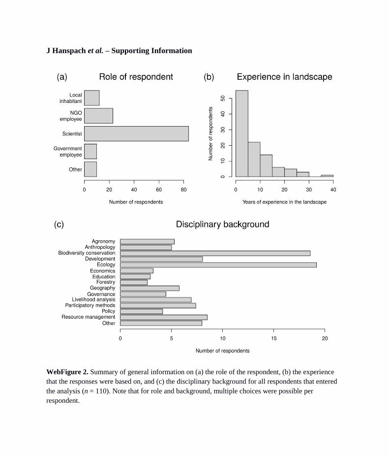
WebFigure 2. Summary of general information on (a) the role of the respondent, (b) the experience

that the responses were based on, and (c) the disciplinary background for all respondents that entered

the analysis (n = 110). Note that for role and background, multiple choices were possible per

respondent.

J Hanspach et al. – Supporting Information

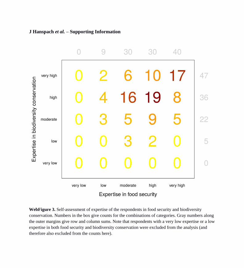
WebFigure 3. Self-assessment of expertise of the respondents in food security and biodiversity

conservation. Numbers in the box give counts for the combinations of categories. Gray numbers along

the outer margins give row and column sums. Note that respondents with a very low expertise or a low

expertise in both food security and biodiversity conservation were excluded from the analysis (and

therefore also excluded from the counts here).

J Hanspach et al. – Supporting Information

WebFigure 4. Food security and biodiversity conservation variables were analyzed using non-linear

principal component analyses, and the first components were extracted from each of the ordinations.

Category centroids along these first components are shown for the single variables of (a) food security

and (b) biodiversity conservation. Categories 1 to 5 correspond to a Likert scale from strongly disagree

to strongly agree for the corresponding statements (see complete statements in WebPanel 1). All

variables except “Utilization” and “Extinction of functional groups” show a strong positive association

with the components for food or biodiversity, respectively. Ticks along the axes give the distribution

of data points.

J Hanspach et al. – Supporting Information

WebFigure 5. Rotated non-linear PCA of biophysical system characteristics. Axis 1 described a

gradient from degraded landscapes (negative values; left-hand side of the graph) to un-degraded

landscapes with clean water and few invasive species (positive values; right-hand side of the graph).

Axis 2 described a gradient from landscapes in mountainous areas with highly variable rainfall

(negative values) to landscapes in flat areas with reliable rainfall (positive values). Biome entered the

analysis as a categorical variable and level centroids are shown in gray. Individual items are

(clockwise from top; Question numbers refer to WebPanel 1): Biome (Question 2.3), Rainfall

variability (Question 5.1), Soil degradation (Question 5.3), Water pollution (Question 5.2), Invasive

species (Question 5.4), and Topography (Question 2.4).

J Hanspach et al. – Supporting Information

WebFigure 6. Rotated non-linear PCA of socio-demographic characteristics. Axis 1 described a

gradient from landscapes where many men and women attended secondary school to landscapes with

low secondary school attendance by both men and women (positive to negative values). Axis 2

described a gradient from landscapes with many children and population growth to landscapes with a

population decrease and emigration (from negative to positive values). Individual items are (clockwise

from top): Emigration (Question 5.8), Women second school (women’s attendance of secondary

school; Question 5.7), Men second school (Question 5.6), Many children (Question 5.5), and

Population change (Question 5.9).

J Hanspach et al. – Supporting Information

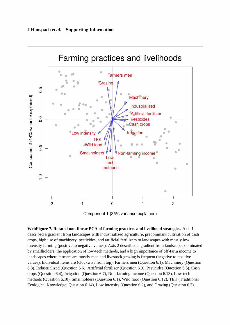
WebFigure 7. Rotated non-linear PCA of farming practices and livelihood strategies. Axis 1

described a gradient from landscapes with industrialized agriculture, predominant cultivation of cash

crops, high use of machinery, pesticides, and artificial fertilizers to landscapes with mostly low

intensity farming (positive to negative values). Axis 2 described a gradient from landscapes dominated

by smallholders, the application of low-tech methods, and a high importance of off-farm income to

landscapes where farmers are mostly men and livestock grazing is frequent (negative to positive

values). Individual items are (clockwise from top): Farmers men (Question 6.1), Machinery (Question

6.8), Industrialized (Question 6.6), Artificial fertilizer (Question 6.9), Pesticides (Question 6.5), Cash

crops (Question 6.4), Irrigation (Question 6.7), Non-farming income (Question 6.13), Low-tech

methods (Question 6.10), Smallholders (Question 6.1), Wild food (Question 6.12), TEK (Traditional

Ecological Knowledge; Question 6.14), Low intensity (Question 6.2), and Grazing (Question 6.3).

J Hanspach et al. – Supporting Information

WebFigure 8. Rotated non-linear PCA of food flows. Axis 1 described a gradient of landscapes

where food import is frequent to landscapes where food is mainly produced within the area (positive to

negative values). Axis 2 described a gradient from landscapes that receive food aid to landscapes

exporting food. Individual items are (clockwise from top): Food export (Question 7.2), Food import

(Question 7.3), Food aid (Question 7.4), and Food from within (Question 7.1).

J Hanspach et al. – Supporting Information

WebFigure 9. Rotated non-linear PCA of governance. Axis 1 described a gradient of a general

increase of governments listening to local people and being engaged in improving biodiversity

conservation and food security (negative to positive values). Axis 2 described a gradient of increasing

effectiveness of conservation, increasing influence of international corporations, global social

movements, research and certification as well as a general stability (negative to positive values).

Individual items are (clockwise from top): Research (Question 7.9), Certification (Question 7.10),

Stable govt (ie stable governance system; Question 7.13), Global social movements (Question 7.8),

Govt listens (Question 7.7), Govt food security (Question 7.5), Govt biodiv conservation (Question

7.6), Effective conservation (Question 7.12), and Corporations (Question 7.11).

J Hanspach et al. – Supporting Information

WebFigure 10. Rotated non-linear PCA of justice. Axis 1 described a gradient of increasing equity

and land access for locals (negative to positive values). Axis 2 described a gradient from landscapes

with good land access for external investors to landscapes with secure land tenure and a high

community spirit (negative to positive values). Individual items are (clockwise from top): Land tenure

(Question 8.5), Land access (Question 8.2), Equity (Question 8.1), Investor access (Question 8.3), and

Community spirit (Question 8.4).

J Hanspach et al. – Supporting Information

WebFigure 11. Rotated non-linear PCA of capital assets. Axis 1 described a gradient of increasing

market access, infrastructure, and financial resources (negative to positive values). Axis 2 described a

gradient of increasing awareness of natural capital, increasing knowledge and health, and a larger role

of traditions (negative to positive values). Individual items are (clockwise from top): Knowledge

(Question 8.6), Health (Question 8.7), Traditions (Question 8.12), Remittances (Question 8.9),

Infrastructure (Question 8.10), Market access (Question 8.11), Financial resources (Question 8.8), and

Awareness natural capital (Question 8.13).

J Hanspach et al. – Supporting Information

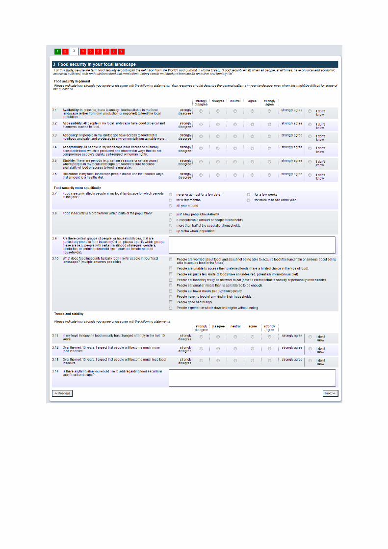
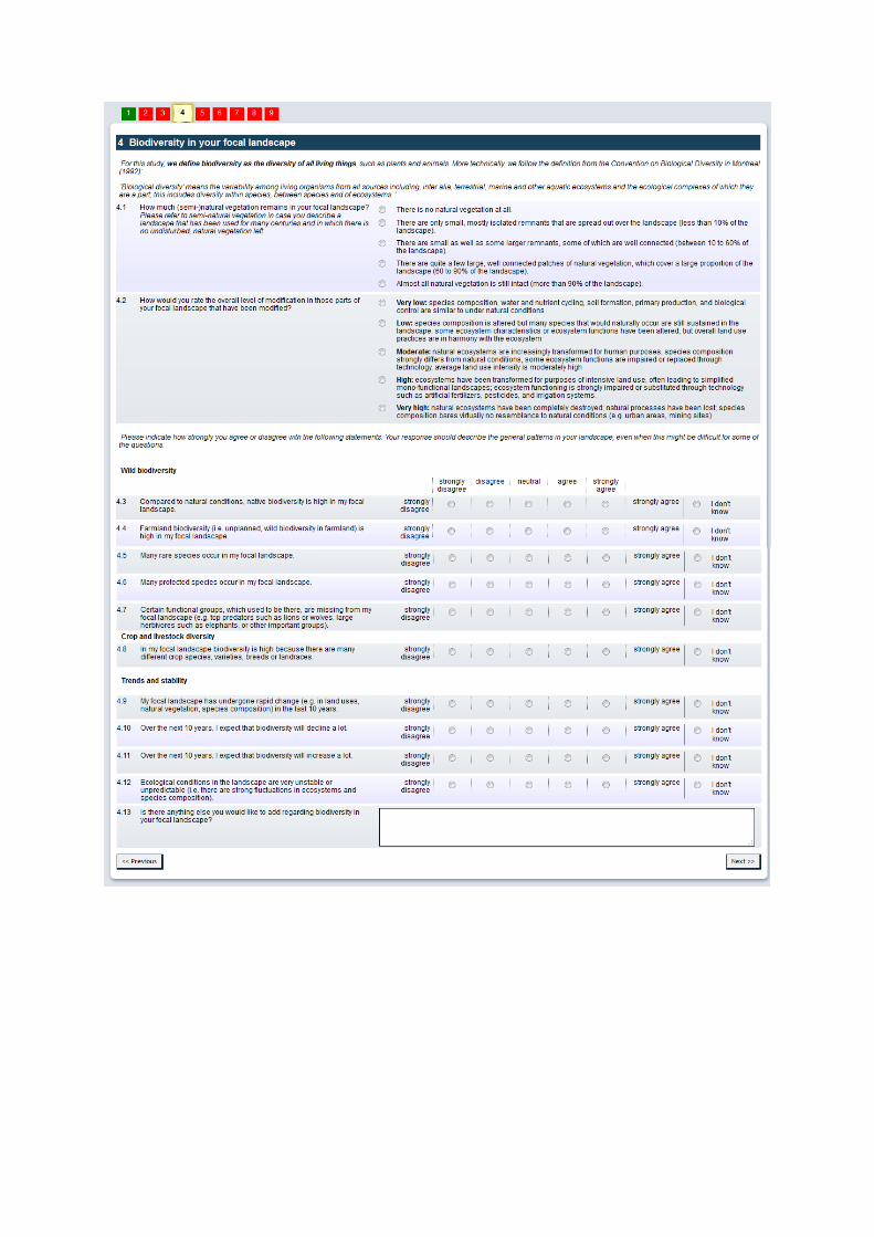
WebPanel 1. Questionnaire

Screen shots of the survey tool on food security, biodiversity conservation, and social–

ecological system characterstics

J Hanspach et al. – Supporting Information

WebPanel 2. Materials and methods

We applied an integrated social–ecological approach in order to assess the interconnected challenge of

achieving food security and biodiversity conservation. The theoretical foundation of this approach was

laid out by Wittman et al. (2017). Briefly, the approach is based on empirical evidence showing that

both food security and biodiversity are driven by a wide range of societal and ecological factors, and

that variables at small scales (eg household, community, patch, or landscape level) are shaped and

constrained by variables operating at larger scales (ie regional, national, and global levels). While a

range of datasets is readily available at coarse scales (eg national-level FAO statistics), disaggregation

to finer scales is generally not possible. Data with a finer resolution usually come from model results

or from downscaling national-level data (Delzeit et al. 2017). Given the ecological and sociopolitical

heterogeneity of most nations, though, existing approaches do not allow a differentiated assessment of

landscape-scale social–ecological interactions. However, as shown by Wittman et al. (2017),

landscapes are a particularly useful analytical unit at which to consider the intersection of food

security and biodiversity conservation. To circumvent common limitations associated with

downscaling national-level data, we collected detailed landscape-scale data through an innovative,

theoretically grounded, expert survey.

Data collection

We conducted an online survey on (1) food security, (2) biodiversity conservation, and (3) social–

ecological system characteristics, focusing exclusively on farming landscapes that are potentially food

insecure (ie in developing countries). The survey was addressed to anyone with expertise on a specific

landscape and on issues related to food security and/or biodiversity conservation in that landscape.

That is, the survey was not limited to academics and researchers, but was open to all individuals with

relevant local expertise (eg conservation practitioners, development agents, or NGO workers).

Respondents were required to answer the survey considering one specific focal landscape on which

they had expert knowledge. The survey consisted of 85 questions grouped into four main sections. The

first section asked for a short characterization of the focal landscape and for a self-assessment of the

respondent’s expertise in relation to that landscape. The second and third sections covered the degree

of food insecurity and biodiversity conservation, respectively, in the focal landscape. Based on

Wittman et al. (2017), the final section covered a wide range of social–ecological system

characteristics of the focal landscape. Most questions consisted of statements that had to be answered

on a five-point Likert scale describing different levels of agreement from “strongly disagree” to

“strongly agree”. The survey was widely distributed via email lists and social networks in order to

reach a wide range of experts. The survey was anonymous and accessible for three months from 15

Nov 2015 to 15 Feb 2016. We received 223 responses. Screen shots of the full original survey tool are

available (WebPanel 1).

Data handling Survey data were subject to extensive data screening and quality control. We excluded all cases with a

self-assessed expertise of “very low” for either food security (n = 4) or biodiversity conservation (n =

4), and as “low” for both (n = 3). Also, we screened the data for plausibility and excluded one case

where most of the questions were answered with “very high”. We excluded 36 cases from developed

countries, because no food insecurity was reported, or obesity and malnutrition (but not

undernutrition) were stated as major problems. Further, we received a disproportionally large amount

of responses for landscapes in Ethiopia (n = 57), from which we randomly sub-selected six cases in

order to avoid bias. (A possible reason for the large number of responses from Ethiopia is that we have

a strong research network there.) Other reasons for the exclusion of landscapes were a focus on urban

areas (n = 11), extensive missing data (n = 4), and study systems with a spatial extent larger than what

we had defined in the survey tool (n = 3). Our final dataset contained 110 cases from 49 countries and

more than ten different biomes (see WebFigure 1 for a map).

We conducted data imputation for 35 cells with missing data (0.5% of all data points). Any

given variable had at most three cells with missing data: that is, less than 3% of data points per

variable. Missing data were imputed with a “neutral” response to avoid a bias in the variables.

Data analysis

First, we extracted the main gradients for food security and biodiversity conservation by applying non-

linear principal components analysis (NLPCA) (Gifi 1990) to each of the datasets. NLPCA uses

optimal scaling and is therefore suitable for ordinally scaled variables such as those measured on a

Likert scale. For food security, NLPCA was performed on the statements on food availability,

accessibility, adequacy, acceptability, stability, and utilization (Questions 3.1–3.6; see WebPanel 1).

The first axis of the NLPCA was extracted and used as a response variable in subsequent analysis.

Similarly, we derived the first component of a NLPCA on the responses for native biodiversity,

farmland biodiversity, protected species, rare species, functional groups, and planned biodiversity

(Questions 4.3–4.8) in order to derive a single indicator of biodiversity. The responses for the negative

statement on the absence of functional groups were reversed before analysis.

Second, to extract the main information on social–ecological characteristics, we also

performed NLPCAs separately for the different themes of social–ecological characteristics (ie

biophysical characteristics, sociodemographics, farming practices and livelihood strategies, food

flows, governance, justice, and capital assets). We extracted the first two axes of each of the seven

NLPCAs (WebFigures 5–11) and applied a varimax rotation in order to improve interpretability of the

axes. Subsequently, we related the rotated axes describing the system characteristics to the axes of

food security and biodiversity conservation. Because we were interested in the influence of the social–

ecological characteristics on both indicators at the same time, we related the axes of social–ecological

characteristics to food security and biodiversity via fitting isotropic smooth surfaces using generalized

additive models (fixed degree regression splines with 10 knots; Wood 2003). Only models where the

estimate of the smoother term was significantly different from zero (Holm adjusted P < 0.05), and that

explained more than 10% of the deviance in the food security and biodiversity indicators, were

included in the results.

Finally, we summarized the responses to the questions on how food security and biodiversity

conservation might change in the future (Questions 3.12 and 3.13 for food security, and 4.10 and 4.11

for biodiversity). For this, we counted how often respondents “agreed” or “strongly agreed” that these

would improve or worsen in the next 10 years and plotted the counts in a circular diagram to visualize

the expected trends.

WebReferences

Delzeit R, Zabel F, Meyer C, and Václavík T. 2017. Addressing future trade-offs between biodiversity

and cropland expansion to improve food security. Reg Environ Change 17: 1429–41.

Gifi A. 1990. Nonlinear multivariate analysis. New York, NY: Wiley.

Wittman H, Abson DJ, Kerr RB, et al. 2017. A social–ecological perspective on harmonizing food

security and biodiversity conservation. Reg Environ Change 17: 1291–301.

Wood SN. 2003. Thin plate regression splines. J Roy Stat Soc B 65: 95–114.