APRIL 2018 Weighted and Unweighted Correlation Methods for Large- Scale Educational Assessment: wCorr Formulas AIR - NAEP Working Paper #2018-01 NCES Data R Project Series #02 Paul Bailey, American Institutes for Research Ahmad Emad, American Institutes for Research Ting Zhang, American Institutes for Research Qingshu Xie, MacroSys Emmanuel Sikali, National Center for Education Statistics The research contained in this working paper was commissioned by the National Center for Education Statistics (NCES). It was conducted by the American Institutes for Research (AIR) in the framework of the Education Statistics Services Institute Network (ESSIN) Task Order 14: Assessment Division Support (Contract No. ED-IES-12-D-0002/0004) which supports NCES with expert advice and technical assistance on issues related to the National Assessment of Educational Progress (NAEP). AIR is responsible for any error that this report may contain. Mention of trade names, commercial products, or organizations does not imply endorsement by the U.S. Government.
Transcript
APRIL 2018
Weighted and Unweighted Correlation Methods for Large-Scale Educational Assessment: wCorr Formulas AIR - NAEP Working Paper #2018-01 NCES Data R Project Series #02
Paul Bailey, American Institutes for Research Ahmad Emad, American Institutes for Research Ting Zhang, American Institutes for Research Qingshu Xie, MacroSys Emmanuel Sikali, National Center for Education Statistics
The research contained in this working paper was commissioned by the National Center for Education Statistics (NCES). It was conducted by the American Institutes for Research (AIR) in the framework of the Education Statistics Services Institute Network (ESSIN) Task Order 14: Assessment Division Support (Contract No. ED-IES-12-D-0002/0004) which supports NCES with expert advice and technical assistance on issues related to the National Assessment of Educational Progress (NAEP). AIR is responsible for any error that this report may contain. Mention of trade names, commercial products, or organizations does not imply endorsement by the U.S. Government.
This page intentionally left blank.
Weighted and Unweighted Correlation Methods for Large-Scale Educational Assessment: wCorr Formulas AIR - NAEP Working Paper #2018-01 NCES Data R Project Series #02
April 2018
Paul Bailey Ahmad Emad Ting Zhang Qingshu Xie Emmanuel Sikali
1000 Thomas Jefferson Street NW Washington, DC 20007-3835 202.403.5000
AIR Established in 1946, with headquarters in Washington, D.C., the American Institutes for Research (AIR) is a nonpartisan, not-for-profit organization that conducts behavioral and social science research and delivers technical assistance both domestically and internationally in the areas of health, education, and workforce productivity. For more information, visit www.air.org.
NCES The National Center for Education Statistics (NCES) is the primary federal entity for collecting and analyzing data related to education in the U.S. and other nations. NCES is located within the U.S. Department of Education and the Institute of Education Sciences. NCES fulfills a Congressional mandate to collect, collate, analyze, and report complete statistics on the condition of American education; conduct and publish reports; and review and report on education activities internationally.
ESSIN The Education Statistics Services Institute Network (ESSIN) is a network of companies that provide the National Center for Education Statistics (NCES) with expert advice and technical assistance, for example in areas such as statistical methodology; research, analysis and reporting; and Survey development. This AIR-NAEP working paper is based on research conducted under the Research, Analysis and Psychometric Support sub-component of ESSIN Task Order 14 for which AIR is the prime contractor. The two other sub-components under Task 14 are Assessment Operations Support and Reporting and Dissemination.
The NCES Project officer for the Research, Analysis and Psychometric Support sub-component of ESSIN Task Order 14 is William Tirre ([email protected]).
The NCES Project officer for the NCES Data R Project is Emmanuel Sikali ([email protected]).
Suggested citation: Bailey, P., Emad, A., Zhang, T., & Xie, Q. (2018). Weighted and Unweighted Correlation Methods for Large-Scale Educational Assessment: wCorr Formulas [AIR-NAEP Working Paper #2018-01, NCES Data R Project Series #02]. Washington, DC: American Institutes for Research.
For inquiries, contact: Paul Bailey, Senior Economist Email: [email protected]
Markus Broer, Project Director for Research under ESSIN Task 14 Email: [email protected]
Mary Ann Fox, Project Director of ESSIN Task 14 Email: [email protected]
Figure 1. Density of Y for Cut Points θ = (−∞,−2,−0.5,1.6,∞). ............................................... 4
Figure 2. Bias Versus ρ for Unweighted Correlations .................................................................... 8
Figure 3. Root Mean Square Error Versus ρ for Unweighted Correlations ................................... 9
Figure 4. Root Mean Square Error Versus Sample Size for Unweighted Correlations ................ 10
Figure 5. Computation time .......................................................................................................... 10
Figure 6. Mean Absolute Deviation Versus ρ (Weighted) ........................................................... 12
Figure 7. Root Mean Square Error vs ρ (Polyserial, Pearson, Polychoric panels) or Population Spearman Correlation Coefficient (Spearman Panel) for Weighted and Unweighted Correlations .............................................................................................................. 13
This page intentionally left blank.
American Institutes for Research Weighted and Unweighted Correlation Methods—1
Introduction The wCorr package can be used to calculate Pearson, Spearman, polyserial, and polychoric correlations, in weighted or unweighted form.1 The package implements the tetrachoric correlation as a specific case of the polychoric correlation and biserial correlation as a specific case of the polyserial correlation. When weights are used, the correlation coefficients are calculated with so called sample weights or inverse probability weights.2
This vignette introduces the methodology used in the wCorr package for computing the Pearson, Spearman, polyserial, and polychoric correlations, with and without weights applied. For the polyserial and polychoric correlations, the coefficient is estimated using a numerical likelihood maximization.
The weighted (and unweighted) likelihood functions are presented. Then simulation evidence is presented to show correctness of the methods, including an examination of the bias and consistency. This is done separately for unweighted and weighted correlations.
Numerical simulations are used to show:
• The bias of the methods as a function of the true correlation coefficient (𝜌𝜌) and thenumber of observations (𝑛𝑛) in the unweighted and weighted cases; and
• The accuracy [measured with root mean squared error (RMSE) and mean absolutedeviation (MAD)] of the methods as a function of 𝜌𝜌 and 𝑛𝑛 in the unweighted andweighed cases.
Note that here “bias” is used for the mean difference between true correlation and estimated correlation.
The wCorr Arguments vignette3 describes the effects the Maximum Likelihood(ML) and fast arguments have on computation and gives examples of calls to wCorr.
Specification of estimation formulas Here we focus on specification of the correlation coefficients between two vectors of random variables that are jointly bivariate normal. We call the two vectors X and Y. The 𝑖𝑖𝑡𝑡ℎ members of the vectors are then called 𝑥𝑥𝑖𝑖 and 𝑦𝑦𝑖𝑖.
1 The estimation procedure used by the wCorr package for the polyserial is based on the likelihood function in Cox, N. R. (1974), "Estimation of the Correlation between a Continuous and a Discrete Variable." Biometrics, 30 (1), pp n171-178. The likelihood function for polychoric is from Olsson, U. (1979) "Maximum Likelihood Estimation of the Polychoric Correlation Coefficient." Psyhometrika, 44 (4), pp 443-460. The likelihood used for Pearson and Spearman is written down in many places. One is the "correlate" function in Stata Corp, Stata Statistical Software: Release 8. College Station, TX: Stata Corp LP, 2003. 2 Sample weights are comparable to pweight in Stata. 3 The wCorr Arguments vignette can be found at https://cran.r-project.org/web/packages/wCorr/vignettes/wCorr Arguments.html
American Institutes for Research Weighted and Unweighted Correlation Methods—2
Formulas for Pearson correlations with and without weights
The weighted Pearson correlation is computed using the formula
where 𝑤𝑤𝑖𝑖 is the weights, 𝑥𝑥 and 𝑦𝑦 are the weighted mean of the X and Y respectively, and 𝑛𝑛 is the number pairs (𝑥𝑥𝑖𝑖 ,𝑦𝑦𝑖𝑖).4
The unweighted Pearson correlation is calculated by setting all of the weights to one.
Formulas for Spearman correlations with and without weights
For the Spearman correlation coefficient the unweighted coefficient is calculated by ranking the data and then using those ranks to calculate the Pearson correlation coefficient—so the ranks stand in for the X and Y data. Again, similar to the Pearson, for the unweighted case the weights are all set to one.
For the unweighted case the highest rank receives a value of 1 and the second highest 2, and so on down to the 𝑛𝑛𝑡𝑡ℎ value. In addition, when data are ranked, ties must be handled in some way. The chosen method is to use the average of all tied ranks. For example, if the second and third rank units are tied then both units would receive a rank of 2.5 (the average of 2 and 3).
For the weighted case there is no commonly accepted weighted Spearman correlation coefficient. Stata does not estimate a weighted Spearman and SAS neither documents nor cites their methodology in either of the corr or freq procedures.
The weighted case presents two issues. First, the ranks must be calculated. Second, the correlation coefficient must be calculated.
Calculating the weighted rank for an individual level is done via two terms. For the 𝑗𝑗th element the rank is
𝑟𝑟𝑟𝑟𝑛𝑛𝑘𝑘𝑗𝑗 = 𝑟𝑟𝑗𝑗 + 𝑏𝑏𝑗𝑗
The first term 𝑟𝑟𝑗𝑗 is the sum of all weights W less than or equal to this value of the outcome being ranked (𝜉𝜉𝑗𝑗)
4 See the "correlate" function in Stata Corp, Stata Statistical Software: Release 8. College Station, TX: Stata Corp LP, 2003.
American Institutes for Research Weighted and Unweighted Correlation Methods—3
Where
𝑤𝑤𝑖𝑖 is the 𝑖𝑖th weight and 𝜉𝜉𝑖𝑖 and 𝜉𝜉𝑗𝑗 are the 𝑖𝑖th and 𝑗𝑗th value of the vector being ranked, respectively.
The term 𝑏𝑏𝑗𝑗 then serves two roles: making the ranks start with one (when there are no ties) and making the ranks the average of the ties (when there are ties).
When there are ties, each unit receives the mean rank for all of the tied units. In the simplest case the weights are all one and there are 𝑛𝑛 tied units the vector of tied ranks would be 𝐯𝐯 =
. The mean of this vector (here called 𝑟𝑟𝑟𝑟𝑛𝑛𝑘𝑘1 to indicate it is a specific case of 𝑟𝑟𝑟𝑟𝑛𝑛𝑘𝑘 when the weights are all one) is then
Where
where the superscript one is again used to indicate that this is only for the unweighted case where all weights are set to one.
Performing an analogous computation as above, the total number of units tied for this rank is taken to be the sum of all of the weights. And the average of these ranks is then taken to be that value divided by the number of sample units tied for this rank. So
where 𝑤𝑤𝑗𝑗 is the mean weight of all of the tied units. It is easy to see that if 𝑤𝑤𝑗𝑗 = 1 for all 𝑗𝑗 then 𝑏𝑏𝑤𝑤 𝑗𝑗 = 𝑏𝑏1𝑗𝑗 .
American Institutes for Research Weighted and Unweighted Correlation Methods—4
After the X and Y vectors are ranked, they are plugged into the weighted Pearson correlation coefficient formula shown earlier.
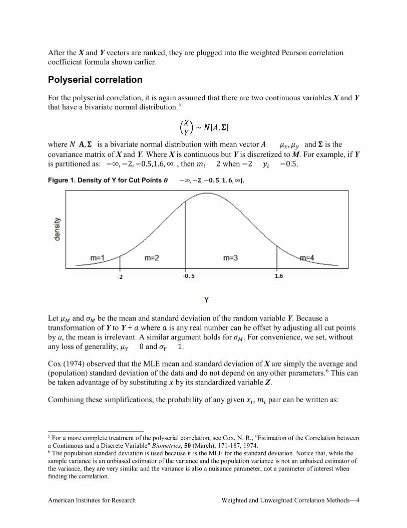
Polyserial correlation
For the polyserial correlation, it is again assumed that there are two continuous variables X and Y that have a bivariate normal distribution.5
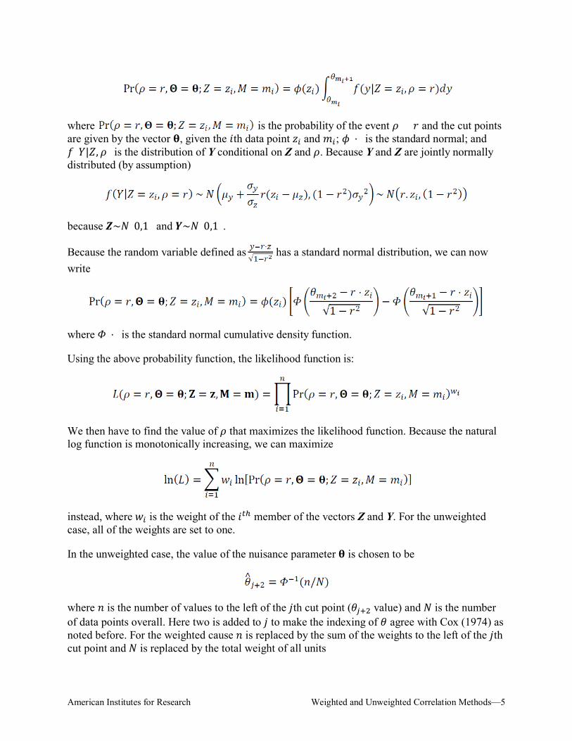
where 𝑁𝑁(𝐀𝐀,𝚺𝚺) is a bivariate normal distribution with mean vector 𝐴𝐴 = (𝜇𝜇𝑥𝑥, 𝜇𝜇𝑦𝑦) and 𝚺𝚺 is the covariance matrix of X and Y. Where X is continuous but Y is discretized to M. For example, if Y is partitioned as: (−∞,−2,−0.5,1.6,∞), then 𝑚𝑚𝑖𝑖 = 2 when −2 < 𝑦𝑦𝑖𝑖 < −0.5.
Figure 1. Density of Y for Cut Points 𝜽𝜽 = (−∞,−𝟐𝟐,−𝟎𝟎.𝟓𝟓,𝟏𝟏.𝟔𝟔,∞).
Let 𝜇𝜇𝑀𝑀 and 𝜎𝜎𝑀𝑀 be the mean and standard deviation of the random variable Y. Because a transformation of Y to Y + 𝑟𝑟 where 𝑟𝑟 is any real number can be offset by adjusting all cut points by a, the mean is irrelevant. A similar argument holds for 𝜎𝜎𝑀𝑀. For convenience, we set, without any loss of generality, 𝜇𝜇𝑌𝑌 = 0 and 𝜎𝜎𝑌𝑌 = 1.
Cox (1974) observed that the MLE mean and standard deviation of X are simply the average and (population) standard deviation of the data and do not depend on any other parameters.6 This can be taken advantage of by substituting 𝑥𝑥 by its standardized variable Z.
Combining these simplifications, the probability of any given 𝑥𝑥𝑖𝑖, 𝑚𝑚𝑖𝑖 pair can be written as:
5 For a more complete treatment of the polyserial correlation, see Cox, N. R., "Estimation of the Correlation between a Continuous and a Discrete Variable" Biometrics, 50 (March), 171-187, 1974. 6 The population standard deviation is used because it is the MLE for the standard deviation. Notice that, while the sample variance is an unbiased estimator of the variance and the population variance is not an unbaised estimator of the variance, they are very similar and the variance is also a nuisance parameter, not a parameter of interest when finding the correlation.
American Institutes for Research Weighted and Unweighted Correlation Methods—5
where is the probability of the event 𝜌𝜌 = 𝑟𝑟 and the cut points are given by the vector 𝛉𝛉, given the 𝑖𝑖th data point 𝑧𝑧𝑖𝑖 and 𝑚𝑚𝑖𝑖; 𝜙𝜙(⋅) is the standard normal; and 𝑖𝑖(𝑌𝑌|𝑍𝑍, 𝜌𝜌) is the distribution of Y conditional on Z and 𝜌𝜌. Because Y and Z are jointly normally distributed (by assumption)
because 𝒁𝒁~𝑁𝑁(0,1) and 𝒀𝒀~𝑁𝑁(0,1).
Because the random variable defined as has a standard normal distribution, we can now write
where 𝛷𝛷(⋅) is the standard normal cumulative density function.
Using the above probability function, the likelihood function is:
We then have to find the value of 𝜌𝜌 that maximizes the likelihood function. Because the natural log function is monotonically increasing, we can maximize
instead, where 𝑤𝑤𝑖𝑖 is the weight of the 𝑖𝑖𝑡𝑡ℎ member of the vectors Z and Y. For the unweighted case, all of the weights are set to one.
In the unweighted case, the value of the nuisance parameter 𝛉𝛉 is chosen to be
where 𝑛𝑛 is the number of values to the left of the 𝑗𝑗th cut point (𝜃𝜃𝑗𝑗+2 value) and 𝑁𝑁 is the number of data points overall. Here two is added to 𝑗𝑗 to make the indexing of 𝜃𝜃 agree with Cox (1974) as noted before. For the weighted cause 𝑛𝑛 is replaced by the sum of the weights to the left of the 𝑗𝑗th cut point and 𝑁𝑁 is replaced by the total weight of all units
American Institutes for Research Weighted and Unweighted Correlation Methods—6
Because the numerical optimization is not perfect when the correlation is in a boundary condition (𝜌𝜌 ∈ {−1,1}), a check for perfect correlation is performed before the above optimization by simply examining if the values of X and M have weekly agreeing order (or opposite but agreeing order) and then the MLE correlation of 1 (or -1) is returned. Where weak agreement means that there is no disagreement—allowing for M to have different associated values of X.
Polychoric correlation
As with the polyserial correlation, the polychoric correlation is a simple case of two continuous variables X and Y that have a bivariate normal distribution. But now both variables are discretized. The continuous (latent) variable Y was observed as a discretized variable M and the continuous (latent) variable X is discretized into P.
The random variable P has the same properties as the M defined above.
Then the probability of any given pair (𝑚𝑚𝑖𝑖 ,𝑝𝑝𝑖𝑖) is
where 𝜌𝜌 is the correlation coefficient, 𝜃𝜃 is the cut points for M and 𝜃𝜃′ is the cut points for P.
Using the probability, the log-likelihood is defined using the same logic as above. The natural logarithm of the likelihood function is then
is then maximized. This is the weighted log-likelihood function. For the unweighted case set the weights to one.
Again, extreme values (correlations of 1 or -1) can be detected by testing for weakly ascending or descending associations between the discrete variables.
Simulation results It is easy to prove the consistency of the 𝛉𝛉 for the polyserial correlation and 𝛉𝛉 and 𝛉𝛉′ for the polychoric correlation using the non-ML case. Similarly, for 𝜌𝜌, because it is a MLE that can be obtained by taking a derivative and setting it equal to zero, the results are asymptotically unbiased and obtain the Cramer-Rao lower bound.
American Institutes for Research Weighted and Unweighted Correlation Methods—7
This does not speak to the small sample properties of these correlation coefficients. Previous work has described their properties by simulation; and that tradition is continued below.7
Simulation study of unweighted correlations
In what follows, when the exact method of selecting a parameter (such as 𝑛𝑛) is not noted in the above descriptions, it is described as part of each simulation.
For each iteration (the exact number of times will be stated for each simulation), the following procedure is used:
• select a true Pearson correlation coefficient 𝜌𝜌;
• select the number of observations 𝑛𝑛;
• generate X and Y to be bivariate normally distributed using a pseudo-Random NumberGenerator (RNG);
• using a pseudo-RNG, select the number of bins for M and P (𝑡𝑡 and 𝑡𝑡′) independantlyfrom the set {2, 3, 4, 5};8
• select the bin boundaries for M and P (𝛉𝛉 and 𝛉𝛉′) by sorting the results of (𝑡𝑡 − 1) and(𝑡𝑡′ − 1) draws, respectively, from a normal distribution using a pseudo-RNG;
• confirm that at least 2 levels of each of M and P are occupied (if not, return to previousstep); and
• calculate and record relevant statistics.
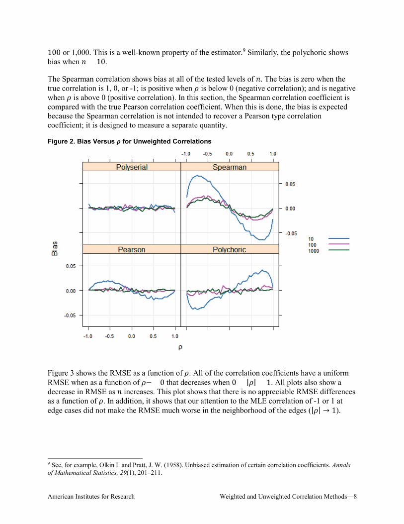
Bias, and RMSE of the unweighted correlations
This section shows the bias of the correlations as a function of the true correlation coefficient, 𝜌𝜌.
A simulation that consist of fifty computations, was done for is pair (𝜌𝜌,𝑛𝑛) where 𝜌𝜌 ∈(−0.99,−0.95,−0.90,−0.85, . . . , 0.95, 0.99), and 𝑛𝑛 ∈ {10,100,1000}.
The bias and the RSME defined respectively as and where the
true correlation coefficient is 𝜌𝜌𝑖𝑖 and estimate correlation coefficient 𝑟𝑟𝑖𝑖 were evaluated for the spearman, polyserial, polychoric and spearman correlations.
Figure 2 shows the bias as a function of the true correlation 𝜌𝜌. The simulation study shows that only the polyserial shows no bias at any level of 𝑛𝑛, shown by no clear deviation from 0 at any level of 𝜌𝜌. For the Pearson correlation there is bias when 𝑛𝑛 = 10 that is not present when 𝑛𝑛 =
7 See, for example, the introduction to Rigdon, E. E. and Ferguson C. E., "The Performance of the Polychoric Correlation Coefficient and Selected Fitting Functions in Confirmatory Factor Analysis With Ordinal Data" Journal of Marketing Research 28 (4), pp. 491-497. 8 This means that the simulation uses discrete ordinal variables (M and P) that have 2, 3, 4, or 5 discrete levels. Note that the number of levels in M and P are chosen independently so that one could be 2 while the other is 5 (or any other possible combination).
American Institutes for Research Weighted and Unweighted Correlation Methods—8
100 or 1,000. This is a well-known property of the estimator.9 Similarly, the polychoric shows bias when 𝑛𝑛 = 10.
The Spearman correlation shows bias at all of the tested levels of 𝑛𝑛. The bias is zero when the true correlation is 1, 0, or -1; is positive when 𝜌𝜌 is below 0 (negative correlation); and is negative when 𝜌𝜌 is above 0 (positive correlation). In this section, the Spearman correlation coefficient is compared with the true Pearson correlation coefficient. When this is done, the bias is expected because the Spearman correlation is not intended to recover a Pearson type correlation coefficient; it is designed to measure a separate quantity.
Figure 2. Bias Versus 𝝆𝝆 for Unweighted Correlations
Figure 3 shows the RMSE as a function of 𝜌𝜌. All of the correlation coefficients have a uniform RMSE when as a function of 𝜌𝜌−> 0 that decreases when 0 < |𝜌𝜌| < 1. All plots also show a decrease in RMSE as 𝑛𝑛 increases. This plot shows that there is no appreciable RMSE differences as a function of 𝜌𝜌. In addition, it shows that our attention to the MLE correlation of -1 or 1 at edge cases did not make the RMSE much worse in the neighborhood of the edges (|𝜌𝜌| → 1).
9 See, for example, Olkin I. and Pratt, J. W. (1958). Unbiased estimation of certain correlation coefficients. Annals of Mathematical Statistics, 29(1), 201–211.
American Institutes for Research Weighted and Unweighted Correlation Methods—9
Figure 3. Root Mean Square Error Versus 𝝆𝝆 for Unweighted Correlations
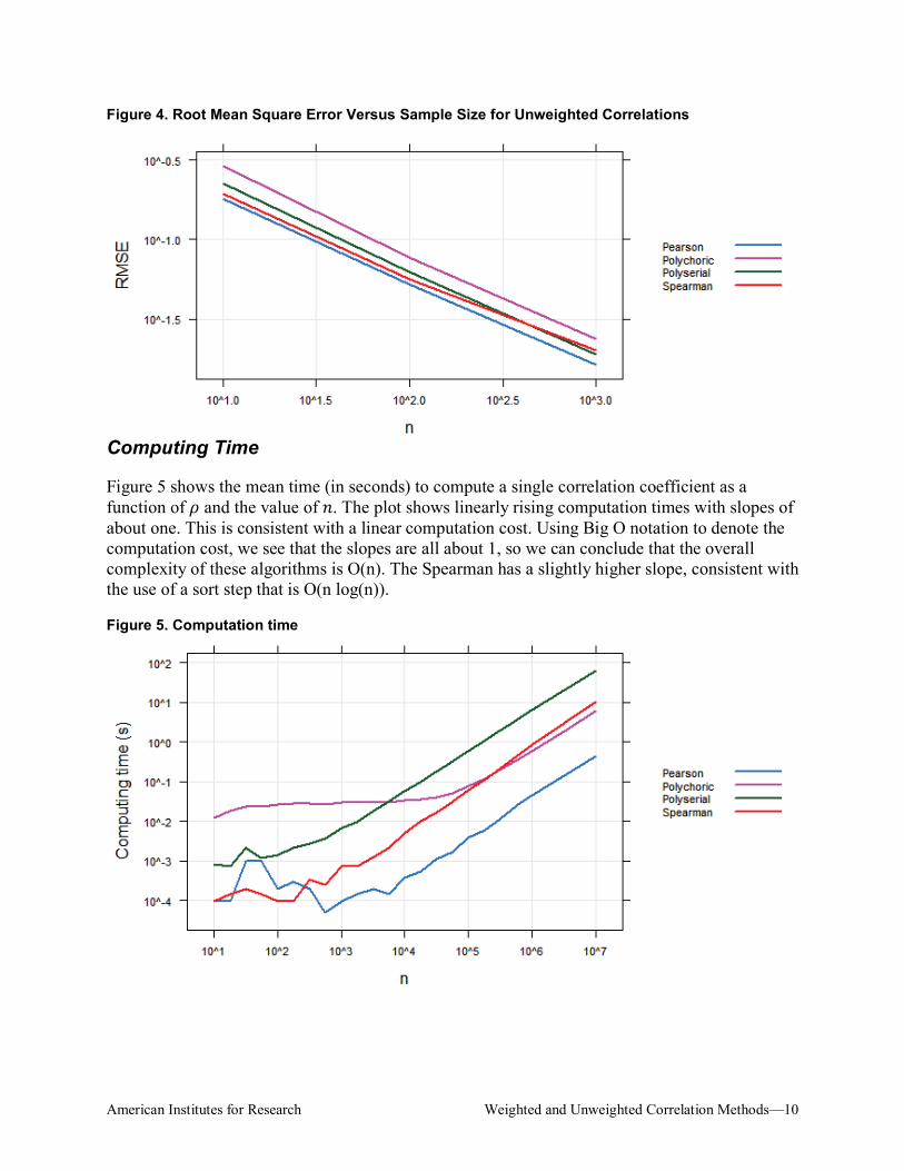
Consistency of the correlations
Figure 4 shows the RMSE as a function of 𝑛𝑛. The purpose of this plot is not to show an individual value but to show that the estimator is consistent. The plot shows a slope of about −1
2
for the Pearson, polychoric, and polyserial correlations. This is consistent with the expected first order convergence for each correlation coefficient under the assumptions of this simulation. Results for the Spearman also show approximate first order convergence but the slope increases slightly as 𝑛𝑛 increases. Again, the Spearman is not estimating the same quantity as the Pearson and so is expected to diverge.
The plot also shows that the RMSE is less than 0.1 for all methods when 𝑛𝑛 > 100.
American Institutes for Research Weighted and Unweighted Correlation Methods—10
Figure 4. Root Mean Square Error Versus Sample Size for Unweighted Correlations
Computing Time
Figure 5 shows the mean time (in seconds) to compute a single correlation coefficient as a function of 𝜌𝜌 and the value of 𝑛𝑛. The plot shows linearly rising computation times with slopes of about one. This is consistent with a linear computation cost. Using Big O notation to denote the computation cost, we see that the slopes are all about 1, so we can conclude that the overall complexity of these algorithms is O(n). The Spearman has a slightly higher slope, consistent with the use of a sort step that is O(n log(n)).
Figure 5. Computation time
American Institutes for Research Weighted and Unweighted Correlation Methods—11
Simulation study of weighted correlations
When complex sampling (other than simple random sampling with replacement) is used, unweighted correlations may or may not be consistent. In this section the consistency of the weighted coefficients is examined.
When generating simulated data, decisions about the generating functions have to be made. These decisions affect how the results are interpreted. For the weighted case, if these decisions lead to something about the higher weight cases being different from the lower weight cases then the test will be more informative about the role of weights. Thus, while it is not reasonable to always assume that there is a difference between the high and low weight cases, the assumption (used in the simulations below) that there is an association between weights and the correlation coefficients serves as a more robust test of the methods in this package.
Results of weighted correlation simulations
Simulations are carried out in the same fashion as previously described but include a few extra steps to accommodate weights. The following changes were made:
• Weights are assigned according to 𝑤𝑤𝑖𝑖 = (𝑥𝑥 − 𝑦𝑦)2 + 1, and the probability of inclusion inthe sample was then .
• For each unit, a uniformly distributed random number was drawn. When that value wasless than the probability of inclusion (Pr𝑖𝑖), the unit was included.
Units were generated until 𝑛𝑛 units were in the sample.
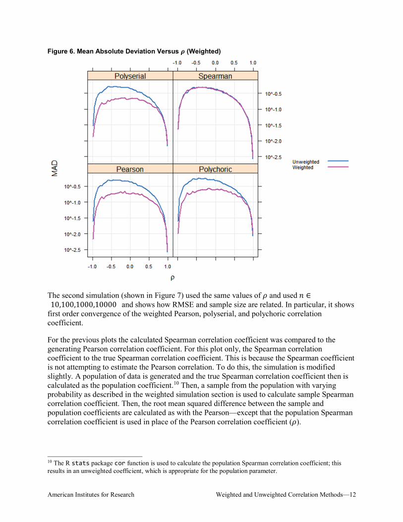
Two simulations were run. The first shows the mean absolute deviation (MAD)
as a function of 𝜌𝜌 and was run for 𝑛𝑛 = 100 and 𝜌𝜌 ∈(−0.99,−0.95,−0.90,−0.85, . . . ,0.95,0.99), with 100 iterations run for each value of 𝜌𝜌.
The following plot shows the MAD for the weighted and unweighted results as a function of 𝜌𝜌 when 𝑛𝑛 = 100. This shows that for values of 𝜌𝜌 near zero, under our simulation assumptions (for all but the Spearman correlation) the weighted correlation performs better than (has lower MAD than) the unweighted correlation for all correlation coefficients. Over the entire range, the difference between the two is never such that the unweighted has a lower MAD. Thus, under the simulated conditions at least, the weighted correlation has lower or approximately equal MAD for every value of the true correlation coefficient (𝜌𝜌).
American Institutes for Research Weighted and Unweighted Correlation Methods—12
Figure 6. Mean Absolute Deviation Versus 𝝆𝝆 (Weighted)
The second simulation (shown in Figure 7) used the same values of 𝜌𝜌 and used 𝑛𝑛 ∈{10,100,1000,10000} and shows how RMSE and sample size are related. In particular, it shows first order convergence of the weighted Pearson, polyserial, and polychoric correlation coefficient.
For the previous plots the calculated Spearman correlation coefficient was compared to the generating Pearson correlation coefficient. For this plot only, the Spearman correlation coefficient to the true Spearman correlation coefficient. This is because the Spearman coefficient is not attempting to estimate the Pearson correlation. To do this, the simulation is modified slightly. A population of data is generated and the true Spearman correlation coefficient then is calculated as the population coefficient.10 Then, a sample from the population with varying probability as described in the weighted simulation section is used to calculate sample Spearman correlation coefficient. Then, the root mean squared difference between the sample and population coefficients are calculated as with the Pearson—except that the population Spearman correlation coefficient is used in place of the Pearson correlation coefficient (𝜌𝜌).
10 The R stats package cor function is used to calculate the population Spearman correlation coefficient; this results in an unweighted coefficient, which is appropriate for the population parameter.
American Institutes for Research Weighted and Unweighted Correlation Methods—13
Thus, the results in Figure 7 show that, when compared to the true Spearman correlation coefficient, the weighted Spearman correlation coefficient is consistent.
In all cases the RMSE is lower for the weighted than the unweighted. Again, the fact that the simulations show that the unweighted correlation coefficient is not consistent does not imply that it will always be that way—only that this is possible for these coefficients to not be consistent.
Figure 7. Root Mean Square Error vs 𝝆𝝆 (Polyserial, Pearson, Polychoric panels) or Population Spearman Correlation Coefficient (Spearman Panel) for Weighted and Unweighted Correlations
Conclusion Overall, the simulations show first-order convergence for each unweighted correlation coefficient with an approximately linear computation cost. Further, under our simulation assumptions, the weighted correlation performs better than (that is, has lower MAD or RMSE than) the unweighted correlation for all correlation coefficients.
We show the first-order convergence of the weighted Pearson, polyserial, and polychoric correlation coefficient. The Spearman is shown to not consistently estimate the population Pearson correlation coefficient but is shown to consistently estimate the population Spearman correlation coefficient—under the assumptions of our simulation
This page intentionally left blank.
This page intentionally left blank.
ABOUT AMERICAN INSTITUTES FOR RESEARCH
Established in 1946, with headquarters in Washington, D.C.,
American Institutes for Research (AIR) is an independent,
nonpartisan, not-for-profit organization that conducts behavioral
and social science research and delivers technical assistance
both domestically and internationally. As one of the largest
behavioral and social science research organizations in the
world, AIR is committed to empowering communities and
institutions with innovative solutions to the most critical
challenges in education, health, workforce, and international
development.
1000 Thomas Jefferson Street NW Washington, DC 20007-3835 202.403.5000


![Constant Time Weighted Median Filtering for Stereo ... · filling (e.g., [2]), and (unweighted) median filtering (e.g., [18]). Recently, Rhemann et al. [22] adopt weighted me-dian](https://static.documents.pub/doc/80x56/5f9f1dd098a69c7f214c0be5/constant-time-weighted-median-filtering-for-stereo-illing-eg-2-and.jpg)


![Discovering Roles and Anomalies in Graphs: Theory and ...eliassi.org/sdm12tut/sdm12tut_roles_part2_final.pdfReal Graph Patterns unweighted weighted static Newman `02] P01.Power-law](https://static.documents.pub/doc/80x56/5f2ed255fb59005ae1731d56/discovering-roles-and-anomalies-in-graphs-theory-and-real-graph-patterns-unweighted.jpg)


