What drives gasoline taxes? Fay Dunkerley 1 Centre for Economic Studies, KU Leuven, Naamsestraat 69, Leuven, B3000 Belgium. Email: [email protected]. Amihai Glazer University of California---Irvine, Irvine, CA 92617, USA Email: [email protected]Stef Proost Centre for Economic Studies, KU Leuven, Naamsestraat 69, Leuven, B 3000 Belgium. Email: [email protected]. 1 The authors thank B.de Borger, A.de Palma, E.Ooghe and G.Willmann for useful comments on an earlier version. Dunkerley & Proost thank the FWO-Flanders for financial support and C.Heyndrickx for research assistance.
Transcript
What drives gasoline taxes?
Fay Dunkerley1
Centre for Economic Studies, KU Leuven, Naamsestraat 69, Leuven, B3000 Belgium.
1 The authors thank B.de Borger, A.de Palma, E.Ooghe and G.Willmann for useful comments on an earlier version. Dunkerley & Proost thank the FWO-Flanders for financial support and C.Heyndrickx for research assistance.
2
Abstract
Gasoline taxes are the most important tax on car use. The question naturally arises as to what tax would be adopted by a government that responds to the preferences of the public. To address that issue, we begin with the standard Downsian model, where policy is determined by the median voter. This model predicts that as long as the median voter is not a car user, he wants high taxes on road use and a road capacity that maximizes net tax revenues. When he becomes a driver himself, he wants road user taxes that are lower and only increase to control congestion, as well as more road capacity. We then use panel data for 28 countries and find support for our theory. When the median voter becomes a driver, the gasoline tax drops on average by 20%.
Keywords: gasoline taxes, median voter theory, political economy
JEL-classification: H23, R48, Q48, L98, Q52
3
1. INTRODUCTION
Both political and economic factors likely influence tax policy in democratic regimes. It is interesting to consider what gasoline taxes would be adopted when a government responds to the preferences of the electorate. Would gasoline taxes change as the use of cars expands? Luxury goods are taxed by the poor majority, whereas, once the majority are car owners, the tax can reduce the externalities generated by road use, particularly congestion. We treat this question both theoretically and empirically, using international panel data to test a simple theory based on the standard Downsian model, where policy is set by the median voter .
The Downsian model can apply both to elections in which two candidates vie for election, and to referenda. A potential limitation of the Downsian model is that it may apply only to a single issue, with single-peaked preferences. But we shall see that under reasonable assumptions, the Downsian model can apply when voters must decide both on users fees and on investment in road capacity. In the model individuals differ only in their incomes, which determine their demand for car use and their benefit of road use and of road investments. Comparative statics of this simple model (varying aggregate income) generate interesting predictions that may explain the decline of real gasoline taxes over time. More precisely one can predict that at the time the median voter becomes a car owner, the tax on gasoline declines.
Our conclusions would also apply under other views of elections. In particular, under our assumptions the citizen-candidate model (see Besley and Coate (1997) could have the median voter run for office, win election, and determine policy. And rather than let any policy be allowed on the agenda, we could extend the model to consider an agenda setter (as in Romer and Rosenthal 1979). The toll would then not be the one preferred by the median voter; but the qualitative results, such as that the toll will be higher if the median voter is a driver than if he is not, will continue to hold.
In the empirical setting, the determinants of gasoline taxes are of course more complex. Based on theory from Persson et al. (2000), Fredriksson and Millimet (2004) use the propensity scoring method to examine gasoline taxes differ in presidential from parliamentary regimes. They find presidential regimes have lower taxes than parliamentary ones. Besley and Rosen (1998) examine vertical tax externalities by looking at the effect of US federal taxes on state gasoline and cigarette taxes. Goel and Nelson (1999) extend the Hettich and Winer (1988) vote-maximising model of how politicians change tax structure in response to change in pre-tax prices. An empirical test, also using US panel data, indicates that state gasoline taxes decline with pre-tax gasoline prices. In a mainly empirical analysis, Hammer et al. (2004) apply panel data from 21 OECD countries and conclude that higher gasoline consumption leads to lower taxes. Rietveld and Van Woudenberg (2005) use cross-section data to explain taxes via fuel price differences between countries. Results are reported separately for diesel and gasoline. In Europe, fuel taxes increase with per capita income per capital spending by government, but there is no sign that negative externalities lead to higher taxes. Decker and Wohar (2007) look at the diesel tax rather than at the gasoline gas, and so
4
concentrate on the U.S. trucking industry. Industry employment is then the significant explanatory variable: the higher the proportion of freight trucking employment in a state, the lower the diesel tax.
Our approach is consistent with the previous empirical analysis but differs in several ways. Our simple political economy theory allows us to examine the evolution of gasoline taxes with real income (over time), rather than testing a static model. The number of road users (and so gasoline consumption) is determined by the preferences of the median voter, given pre-tax price, average income, and capacity of the roads. In this setting, changes in gasoline taxes can be considered to represent governmental response to the preferences of the median voter as a private road user. Diesel, on the other hand, is more widely used for freight transport. We therefore restrict the empirical analysis to gasoline taxes. The empirical test is applied to 28 democratic countries, controlling for pre-tax price, as this does not remain constant over time. Other determinants, including the structure of political institutions, are accounted for in country-specific fixed effects.
In Section 2 the theoretical model is developed, the empirical analysis is described and discussed in Section 3 before Section 4 concludes.
2. MEDIAN VOTER MODEL
2.1. Theoretical Framework
Consider an area where road capacity is given at a level K and where congestion is more or less homogeneous in the whole area. Assume further that the location of activities is fixed.
Each of a large number, N, of individuals (n=1,..,N) has a share nα in total income Ζ. The richest individual has index 1, the poorest index N. Each of the individuals can choose to own and use a car or not. Let U(x,d)+W(E) be the direct utility of an individual. It is a function of the consumption of other goods x and the use (d=1) or not (d=0) of a car. It also depends on the supply of public goods E that do not relate to transportation. We assume that the public goods not related to transportation are additively separable from the utility of driving. All goods are normal goods.
Let the price of the consumption good be 1 and let the cost of driving be
,dDp a bTK
τ ⎛ ⎞= + + ⎜ ⎟⎝ ⎠
(1)
where a is a fixed resource cost of owning a car, and τ is the tax on car ownership and use. We can call it the gasoline tax. The last term represents the user time cost of using a car and this is a function of the ratio between the total number of car users, D, and the road capacity, K.
5
Consider first an individual’s consumption choice. He decides to own and use a car if he thereby increases his utility. He solves the following problem:
( ) Maximize ( , )
subject to ,with equal to 0 or 1
d n
U x d W Ex p d Z
dα+
+ ≤ (2)
Once d has been chosen, the rest of the income is spent on the consumption good x so that the solution of this problem can be characterised by car ownership as a function of total cost and income: ( , )d nd p Zα , that we assume is continuous and twice differentiable. The decision to own a car will be a function of the price and of income. The total number of drivers D equals
1
( , ) .N
d nD d p Z dn Nα= ≤∫ (3)
As owning and using a car is a normal good we have that 1( , ) ( , )d n d nd p Z d p Zα α− ≥ so when a given individual prefers to own a car, all individuals with higher income (lower index) will also own a car.
We can now introduce a government budget constraint and a political decision making process. We assume a simple set up: government has to pay for general expenditures E and for roads that have a rental cost r and has to finance the expenditures by a proportional income tax t and by the car tax τ. In a first stage, it fixes the income tax t and the level of the other expenditures E. In a second stage it decides on the gasoline tax and on the road capacity. We shall suppose for simplicity that a driver uses a fixed amount of gasoline (so that the length of trips, and the fuel efficiency of cars, is constant2), so that we can refer interchangeably to a tax on road use, a toll on roads, and a gasoline tax. The government budget equation is:
tZ D rK Eτ+ = + (4)
We start the analysis by assuming road capacity is fixed. We relax the fixed road capacity assumption later. We assume that the road taxes are decided by simple majority voting and leave the rest of the political system unspecified3. To balance the
2 This is a simplification to which we return at the end of this section.
3 One could also study the structure of taxes and level of non-road public goods as in Gevers and Proost (1978).
6
government budget equation we assume moreover that the government expenditures remain fixed and that the budget is balanced by a lower income tax. These assumptions reduce the political decision to one dimension: the gasoline tax, knowing that the revenues are returned under the form of lower income taxes. If preferences of each individual over the car use tax are single peaked4 we can study the political equilibrium by analysing the preferences of the median voter.
When the median voter decides on the car tax he compares two options: either he prefers to own a car and recognizes that he must pay a gasoline tax, or he prefers not to own a car and then enjoys the revenue from a gasoline tax.
Assume first that the median voter does not drive. Let the income of the median voter be med Zα . Then he selects the gasoline tax, 0
medτ , that maximizes the following expression:
[ ]1 ,0 ,
subject to / 2.
medrK E DU Z W E
Zn N
τ α⎡ + − ⎤⎛ ⎞− +⎜ ⎟⎢ ⎥⎝ ⎠⎣ ⎦<
(5)
The first-order condition gives the gasoline tax which maximizes revenue from that tax as:
0 ( )med
DDττ
τ
= −∂∂
. (6)
The intuition is straightforward: the median voter is not a car owner so he prefers to minimize his own income tax payments.
2.1.1. Median voter drives
Now consider the case where the median voter prefers to own a car. Then his choice of tax rate 1
medτ involves a more difficult trade off as he seeks to maximise (subject to n>N/2):
4 This can be guaranteed using additional restrictions on preferences.
which implies the following optimal tax on car use
1 ( ) 1 1( )
med
med
D b T DD D K Dττ
τατ τ
∂ ∂⎛ ⎞= − +⎜ ⎟∂ ∂ ∂ ∂⎝ ⎠− −∂ ∂
. (9)
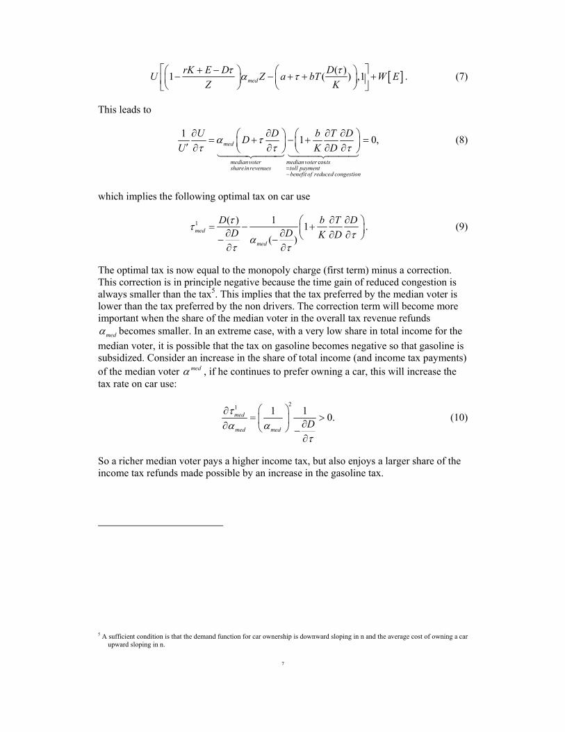
The optimal tax is now equal to the monopoly charge (first term) minus a correction. This correction is in principle negative because the time gain of reduced congestion is always smaller than the tax5. This implies that the tax preferred by the median voter is lower than the tax preferred by the non drivers. The correction term will become more important when the share of the median voter in the overall tax revenue refunds
medα becomes smaller. In an extreme case, with a very low share in total income for the median voter, it is possible that the tax on gasoline becomes negative so that gasoline is subsidized. Consider an increase in the share of total income (and income tax payments) of the median voter medα , if he continues to prefer owning a car, this will increase the tax rate on car use:
21 1 1 0.med
med medD
τα α
τ
⎛ ⎞∂= >⎜ ⎟ ∂∂ ⎝ ⎠ −
∂
(10)
So a richer median voter pays a higher income tax, but also enjoys a larger share of the income tax refunds made possible by an increase in the gasoline tax.
5 A sufficient condition is that the demand function for car ownership is downward sloping in n and the average cost of owning a car upward sloping in n.
8
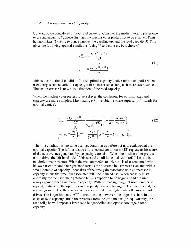
2.1.2. Endogenous road capacity
Up to now, we considered a fixed road capacity. Consider the median voter’s preference over road capacity. Suppose first that the median voter prefers not to be a driver. Then he maximizes (5) using two instruments: the gasoline tax and the road capacity K. This gives the following optimal conditions (using °° to denote the best choices):
00 0000
00 0000
( , )
( , ) .
medD K
D
D KrK
ττ
τττ
= −∂∂
∂=
∂
(11)
This is the traditional condition for the optimal capacity choice for a monopolist when user charges can be varied. Capacity will be increased as long as it increases revenues. The tax on car use is now also a function of the road capacity.
When the median voter prefers to be a driver, the conditions for optimal taxes and capacity are more complex. Maximizing ((7)) we obtain (where superscript 11 stands for optimal choice):
11 11
1111
11 11 11 1111 2
( , ) 1 1( )
' ( , ) .( )
med
med
med
D K b T DD D K D
D bT Dr K D KK K K
τττα
τ τ
τ α τ
∂ ∂⎛ ⎞= − +⎜ ⎟∂ ∂ ∂ ∂⎝ ⎠− −∂ ∂
∂ ∂⎛ ⎞ ⎡ ⎤− + = −⎜ ⎟ ⎢ ⎥∂ ∂⎝ ⎠ ⎣ ⎦
(12)
The first condition is the same user tax condition as before but now evaluated at the optimal capacity. The left-hand side of the second condition in (12) represents his share of the net revenues generated by a capacity extension. When the median voter prefers not to drive, the left-hand side of this second condition equals zero (cf. (11)) as this maximizes net revenues. When the median prefers to drive, he is also concerned with his own user cost and the right-hand term is the decrease in user cost associated with a small increase of capacity. It consists of the time gain associated with an increase in capacity minus the time loss associated with the induced use. When capacity is set optimally for the user, the right-hand term is expected to be negative and the user always gains from an increase in capacity. With decreasing marginal user benefits of capacity extension, the optimum road capacity needs to be larger. The result is that, for a given gasoline tax, the road capacity is expected to be higher when the median voter drives. The larger his share medα in total income, however, the larger his share in the costs of road capacity and in the revenues from the gasoline tax (or, equivalently, the road toll); he will oppose a large road budget deficit and oppose too large a road capacity.
9
2.2. Comparative statics and change over time
We are interested in knowing how the gasoline tax and capacity change over time when overall income grows. For constant costs of road building, we can consider the following comparative static exercise. Assume that aggregate income increases and that the share of the median voter in the total income remains constant when income increases. As using a car is a normal good, one can expect that the number of drivers increases with income. As long as the median voter prefers not to drive, the tax on car use will maximise revenues and road capacity will be decided as a function of this objective. If road construction exhibits constant returns to scale,6 as we assume, and if road capacity is continuously updated, one can expect an increasing tax on car use as overall income grows. This is our first testable proposition:
PROPOSITION I: When the median voter prefers no to drive, when his share in total income remains constant and when capacity and the gasoline tax can be varied continuously, an increase in total income leads to an increase in the tax on road use.
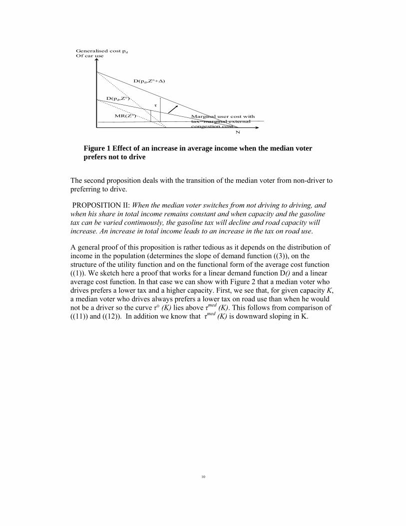
This result can be easily shown using Figure 1. It depicts the upward shift in demand for owning and using a car D(pd,Z) when income increases from Z° to Z°+Δ. We also represent the marginal user cost before taxes. This is a long-run user cost function that is a function of the ratio between demand for car use and capacity. When road construction and maintenance exhibit constant returns to scale, the long-run user cost function including the external congestion tax is constant and revenue from the external congestion tax fully covers the costs of capacity.7 Consider now a median voter that wants to maximise net revenues from road use charges. He will select a number of drivers such that the marginal user cost (including the gasoline tax) equals the marginal revenue (MR). As the demand function rotates upward, this implies that the tax on car use has to rise.
6 See Small & Verhoef (2007, p112) for evidence on economics of scale in road construction.
7 This follows from the fact that the user cost function is homogeneous of degree zero in the ratio D/K and that the rental cost of capacity is assumed constant.
10
N
D(pd,Z°+Δ)
Generalised cost pdOf car use
D(pd,Z°)
Marginal user cost withtax=marginal externalcongestion cost
MR(Z°)
τ
Figure 1 Effect of an increase in average income when the median voter prefers not to drive
The second proposition deals with the transition of the median voter from non-driver to preferring to drive.
PROPOSITION II: When the median voter switches from not driving to driving, and when his share in total income remains constant and when capacity and the gasoline tax can be varied continuously, the gasoline tax will decline and road capacity will increase. An increase in total income leads to an increase in the tax on road use.
A general proof of this proposition is rather tedious as it depends on the distribution of income in the population (determines the slope of demand function ((3)), on the structure of the utility function and on the functional form of the average cost function ((1)). We sketch here a proof that works for a linear demand function D() and a linear average cost function. In that case we can show with Figure 2 that a median voter who drives prefers a lower tax and a higher capacity. First, we see that, for given capacity K, a median voter who drives always prefers a lower tax on road use than when he would not be a driver so the curve τ° (K) lies above τmed (K). This follows from comparison of ((11)) and ((12)). In addition we know that τmed (K) is downward sloping in K.
11
K
τK°(τ) K med (τ)
τ° (K)
τ med (K)
MedianNot a driver
Median is driver
Figure 2 Difference in gasoline tax and capacity between a median voter who drives and a median voter who does not
For a given gasoline tax, the optimal road user capacity K°(τ) when the median voter prefers not to drive is always smaller than when he prefers to drive Kmed (τ). In addition, Kmed (τ) declines with τ. The result is that the solution τ°, K° preferred by a median voter who is not a driver always has a higher gasoline tax and a smaller capacity than when the median voter prefers to drive.
To see the effect of an increase in average income when the median is a driver, we continue to use a linear demand and average cost function. Starting with the optimal tax when the median voter is a driver and keeping capacity constant, an increase in average incomes will increase the number of drivers. In the expression for the optimal user tax (first line in (12)), we see that the first part of this expression related to the revenue generating function of the user tax, increases while the second (negative) part stays constant. So the optimal gasoline tax increases.
This could give a profile for gasoline taxes as presented in Figure 3. At low aggregate income, the median voter is not a driver and favours the revenue-maximizing gasoline tax. When aggregate income rises, the number of users will rise and so will the gasoline tax. Once a certain income is reached, the median voter’s valuation for car trips has become so high that he also wants to drive, and this means he favours a lower tax. When income continues to grow, the number of drivers keeps increasing and the median voter favours an increase in the gasoline tax.
12
AggregateIncome
TollD
Toll selected by medianvoter
Median voter does not drivei d i
Median voter drives
N/2
D
Figure 3 Effect on gasoline tax of an increase in aggregate income when capacity can be continuously adapted
Another candidate for comparative statics is the pre-tax price of gasoline. As oil prices have shown significant variations, this can be important. The pre-tax gasoline price enters the theoretical model via the pre-tax cost of driving parameter, a, in (1). If the median voter prefers not to drive, an increase in the pre-tax price increases the marginal user cost before tax. When tax revenue is the objective, the tax on gasoline will decrease when the pre-tax price increases. This leads us to Proposition 3.
PROPOSITION III. When the median voter prefers not to drive, an increase in the pre-tax price of gasoline leads, ceteris paribus, to a reduction in the gasoline tax.
The proof is straightforward and comes down to an increase in the marginal user cost before tax shown in Figure 1. When demand functions and marginal cost functions are linear, half of the pre-tax price increase would be absorbed in this case of pure monopoly pricing by the government.
PROPOSITION IV. When the median voter becomes a driver, an increase in the pre-tax price of gasoline leads to a decrease in the gasoline tax he prefers.
This can be shown using ((12)). An increase of the average cost implies that the first component of the user charge, the revenue raising component decreases because demand is lower. The second component is constant for linear demand and average cost functions. So the gasoline tax will increase but probably less than when the median voter is a driver.
13
In our theoretical model we kept the energy efficiency and the mileage per car fixed. There is no reason why the comparative statics effects we derived in a simplified model would no longer hold in a model with endogenous car efficiency and endogenous mileage. What matters is that the median voter integrates these reactions into his choice. When the median voter is not a driver he takes into account car efficiency reactions and car mileage reactions. Both effects will increase the price elasticity of gasoline demand and lower the elasticity of the number of drivers with respect to the price of gasoline. The net effect on taxes is an empirical matter but the shift in tax rates when the median driver finds it interesting to become a driver will still be there.
3. EMPIRICAL ANALYSIS
3.1. Data
This section tests whether the median voter model provides a plausible explanation of national policy on taxes for road use by non-commercial vehicles using international panel data. The dataset covers 28 mainly OECD countries8 for the period 1978-2005. In most countries, taxes on road use by non-commercial vehicles consist of fuel taxes and of annual vehicle taxes. Although diesel is being increasingly used by car drivers, particularly in Europe,9 we limit our study to gasoline taxes as these are only imposed on private vehicles and do not extend to commercial vehicles as is the case with diesel. It is reasonable to assume that the behaviour of voters who choose to drive (or not to drive) gasoline cars will be representative of the voting population as a whole. It would be useful to include annual vehicle taxes, as these appear to differ widely between countries10 and depend on vehicle characteristics (vehicle size, power etc), which can be considered to indicate environmental preferences. These tax data, however, were only readily available from 2001 onwards,11 a small part of our sample period, and were
8 Australia, Austria, Belgium, Canada, the Czech Republic, Denmark, Finland, France, Germany, Greece, Hungary, Ireland, Italy Japan, South Korean, Luxembourg, Mexico, the Netherlands, New Zealand, Norway, Poland, Portugal, Slovakia, Spain, Sweden, Switzerland, the United Kingdom and the USA
9 According to Eurostat data, in 2000, more than 30% of cars used diesel in Austria, Belgium, France, Luxembourg and Spain. In other countries, usage was less than 15%.
10 A rough calculation based on total annual vehicle taxes per country for 2000 (source TREMOVE) indicates that vehicle taxes are a similar order of magnitude to gasoline taxes except for Luxemburg, Portugal and Spain, where the ownership tax was very low.
11 Source ACEA
14
therefore not used. As long as their structure does not change, these will be captured in the country fixed effects that we will introduce later.
The fuel tax data are total taxes combining excise, VAT, local and federal taxes, where applicable. Gasoline tax and pre-tax gasoline price data in national currencies per litre were obtained from the IEA (IEA 1998, 2006). Where different grades of gasoline were available, a simple average has been taken. The GDP per capita data, which is used to represent aggregate income, and conversion parameters (CPI and PPP exchange rates) are taken from the OECD Factbook 2008. All data have been converted to US dollars at year 2000 prices. Some limitations to the dataset should be noted: data was not available for all countries for each year and tax data for South Korea was limited (starting only with 2000). For several countries, the conversion to real data resulted in inflated values for a number of years. This could be due to the relatively low average income in these countries or because they were in a period of political transition. Data were therefore excluded for Spain before 1986, Portugal before 1990, Greece before 1992 and for Mexico, the Czech Republic, Hungary, Poland and Slovakia before 1995.
3.2. The empirical model
Propositions 1 and 2 in Section 2 indicate that a uniform increase in incomes generally increases the tax on road use. When a certain average income is reached, the median voter prefers to drive and the gasoline tax falls (see Figure 2). This hypothesis can be tested empirically using an econometric model.
[ ], , 1 , , ,( )i t i t i t i i t k j j i i tj
GDP GDP pg Tτ θτ β γ η λ α ε− −= + + ∂ + + + +∑ . (13)
In equation (13), the subscript i denotes country and the subscript t denotes year. The “time” subscript (t) does play some role in our analysis, although we are not performing a time-series regression as we examine the relationship between taxes and aggregate income, which is represented by GDP per capita( ,i tGDP ). The model, however, can suffer both from serial correlation in the error terms (as the gasoline taxes are correlated in time) and heteroscedasticity (as the variance of the errors may be country-specific). Since the predictions of the median voter model are derived from comparative statics, we include one lag of the dependent variable in the empirical model; this lag is widely seen to adequately characterise many dynamic adjustment processes in economics (e.g.
15
Bun and Kiviet 2006). The presence of autocorrelation in the dataset is confirmed by applying the test developed by Wooldridge (2002).12 The implications of a dynamic panel for the model estimation are discussed in Section 3.4
The data are pooled for all countries, so that GDP per capita ( ,i tGDP ) is assumed to have the same effect on gasoline taxes in all countries; because taxes increase with aggregate income and with the number of drivers, we expect the effect to be positive.
The ( )i GDP∂ term determines how a GDP sufficiently high to make the median voter a driver affects the gasoline tax:
*( ) 1( ) 0
i i i
i
GDP if GDP GDPGDP otherwise
∂ = ≥∂ =
,
where *iGDP denotes the level of GDP at which the median voter becomes a driver.
*iGDP may differ between countries, since the same level of economic development at
which the median voter becomes a driver may also depend on other country-specific factors. However, the regression coefficient should be negative as, for any income level, the median voter favours a lower tax when he drives compared to when he does not. Based on a simple linearised version of the median voter model, this coefficient would be the same in all countries with the same willingness to pay for road use. We therefore use one common coefficient for all countries in the dataset ( iγ γ= ). Clearly the estimation of the *
iGDP variable is important for the estimation of the overall model. We return to this in Section 0 below.
In our static theoretical model, the pre-tax price of gasoline is assumed to be fixed (parameter a in equation (1)). In theory, a consumer government could raise its import tax on gasoline in order to decrease the import price and use its monoposony power, at that moment the before tax price would become endogenous. We take before tax price as given because none of the importing governments has a large share of the market so that an import tax strategy is not very efficient for each of them individually.
Because real prices can vary, we control with a variable giving the inflation-adjusted price of gasoline, ,i tpg .Because governments are unable to implement policy immediately in response to price changes, we expect a lagged effect. In the static model,
12 This is implemented in STATA by xtserial.
16
the tax would be expected to have a negative response to pre-tax price at fixed income, consistent with Goel and Nelson (1999 and Besley and Rosen (1998). In our case, we again distinguish between the two regimes when the median voter prefers to drive or not to drive. Following Proposition 3, if he is not a driver, a revenue maximizer would indeed react to a price increase of fuel by absorbing part of the price increase and reduce the gasoline tax. Also if the median voter is already a driver, the consumers’ price is a mixture of the monopoly tax setting and of regulating congestion and the response to a fuel price increase would be to reduce the tax, as in Proposition 4. In our international panel dataset, however, the observed gasoline tax contains both excise and VAT for all countries except for the US13, so that in the linear regression the derivative of tax with respect to pre-tax price also contains a VAT component. We do not attempt to correct for this, as the VAT rate is a policy variable and is not fixed forever--it can rise or fall just as the excise tax can. There has been some harmonization within the European Union, but this also holds for excise taxes.
Clearly, the pre-tax price of gasoline is influenced by major exogenous events. These are taken account of in our analysis by time dummies ( jT ). Dummies are included for the following years: 1980 and 1991 (US price controls); 1990 (Gulf War); 1998 (OPEC 10% quota increase); 1999 (OPEC production cuts); and 2001 (9/11)14.
Another political consideration, not covered by the median voter theory, but which may influence gasoline taxes, is the timing of elections. Governments may reduce taxes in an election year. But because in every year of our sample some country has an election, and events other than elections can swamp election effects, including time dummies for election years is unlikely to yield useful insights.15
13 For the US, we did not distinguish the different components, as according to the IEA data source: “US Sales of motor fuels to
non-commercial users are generally exempt of the general sales tax because in all states and in some municipalities’ special motor
fuel taxes exist. However in about eight states both taxes are cumulated. The estimates of national weighted average rates and
amounts below take account of this situation as far as possible. In addition to the above a special federal motor fuel tax exists.”
14 Source: WTRG Economics: http://www.wtrg.com/
15 This was confirmed by regressions including one time dummy for each year.
17
Other country-specific, time invariant effects are included in iα . Given the large number of countries used in the analysis, we expect that in the regression we are not controlling for several factors. These country-specific fixed effects represent all other determinants that remain constant within a country such as the structure of political institutions, density, country size, other taxes on vehicle ownership and use, etc. We assume that these are fixed effects rather than random effects as they represent omitted variables and as the panel comprises a large sample of democratic countries with established gasoline tax policies. This is confirmed using a Hausmann test.
The theory outlined in Section 2 is partial in the sense that only a limited number of variables are included, which are considered to be the main determinants of the model and allow us to maintain the assumptions of the Downsian framework. In the empirical analysis, we also mainly restrict ourselves to these major explanatory variables and prefer to incorporate others into the fixed effects. Therefore we do not include in our model several variables, among others gasoline consumption, tax revenue and government expenditure. In the median-voter model, the number of road users, which would translate into gasoline consumption in the empirical analysis, is determined by the median voter’s preferences, given the tax rule, income level, pre-tax price, and road capacity. We would therefore expect gasoline consumption to be highly correlated with GDP per capita and with the price of gasoline.16 Because in our theoretical model we hold government spending fixed, government spending (E) does not play a role in the median voter’s preferences.
3.3. Determining when the median voter drives
Finding *iGDP , the value of GDP at which the median voter becomes a driver, is central
to the model estimation and should ideally be determined endogenously by comparing equations (5) and (7).17 In practice, estimating *
iGDP endogenously would require the introduction of many additional variables, increasing the potential sources of error in the model. The term ( )i GDP∂ is effectively equivalent to modelling a structural break in the country-specific fixed effects. When the timing of a structural break is known, a Chow test can be used to test whether the coefficients estimated by the econometric
16 Indeed Hsing (1994) finds that, for US data, gasoline consumption varies positively with GDP and negatively with pre-tax price and gasoline tax.
17 In a fuller analysis, where both tax and transport investment decisions are made simultaneously, the simultaneity affects the regressions via the GDP level at which the median voter drives. Assuming a fixed capacity level, however, does not qualitatively affect the tax regression results.
18
model are the same before and after the break (e.g. Greene 2008). In the time series literature, tests have been developed to detect endogenous breakpoints in both constant and slope terms (Bai and Perron 1998, Andrews 1993). In a panel data setting, Mohn and Misund (2009) determine the structural change in their model endogenously by finding the break year which maximises the Chow test for the slope coefficients of the independent variables. Obfsgård and Zahran (2008) apply the Bai-Perron algorithm to search for shifts in corruption using time series data for 126 countries. Both Andrews and Lu (2001) and de Wachter and Tzavalis (2004) consider structural breaks in dynamic linear panel data models using GMM estimation techniques. The latter find that the standard Arellano-Bond estimator is robust to uncorrelated changes in fixed effects. However, the above approaches all assume that any structural breaks occur at a common point in time for all panels.
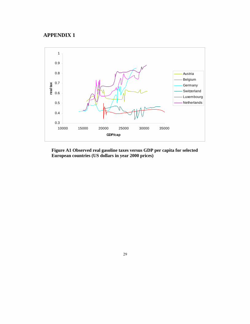
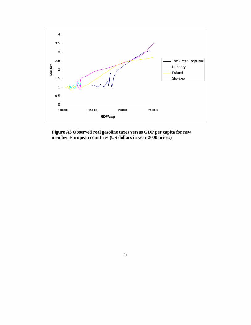
In our model, the break in the fixed effects may occur at different levels of GDP (and different times) for each country, as noted above: a maximisation approach is therefore difficult to apply. The shift in gasoline tax is also predicted by the theory and not the result of exogenous events. We therefore choose to specify the breakpoint before estimating the econometric model and use sensitivity analysis to take account of the accuracy of the GDP* calculation on the modelling results. As a starting point, we consider the evolution in observed gasoline price and tax rates with respect to GDP per capita (see Figures in Appendix 1). Although it is possible to identify a drop in tax rate at a real GDP per capita of roughly 18,000 US dollars in year 2000 prices for several European countries, this is by no means clear cut. For Hungary, the Czech Republic, Poland and Slovakia, the tax seems to follow the pre-tax price trend quite closely. For these we assume that the median voter is not yet driving.
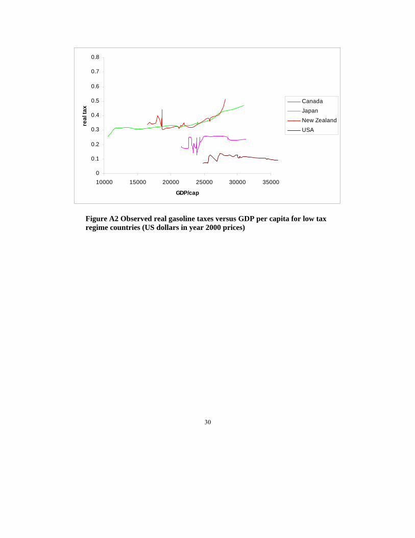
The low-tax countries are Japan, New Zealand, Australia, Canada and the United States. Tax rates for these countries seem to grow independently of the pre-tax price. In these cases we suppose that the median voter is already driving before 1978. For New Zealand, Australia and Canada congestion is probably not a problem on a national scale, although congestion is undoubtedly present in large conurbations.
A second approach is to use an independent dataset on car ownership data to determine the GDP level at which the median voter becomes a driver. In this case, annual vehicle fleet data18 and annual population data (OECD 2008) for each country were used to determine the year when more than half the voting adults were car owners. Data were available for 1970 to 2007 with some gaps. The population data were adjusted for
18 Data provided by International Transport Forum.
19
family size19 (source OECD family database and EEA) and the number of voting adults per household.20 It was further assumed that passenger vehicles account for a fixed percentage (80%) of the fleet (these last data are not country or year specific). A simple division then yields the number of vehicles per voting adult in each year and the year in which the median voter became a car owner. The corresponding GDP then had to be inferred from the year using OECD data. Because real GDP does not necessarily increase monotonically over time for all countries, we must allow some latitude.
Table 1 shows the resulting GDP* values. We see that when the car ownership dataset is used, fourteen countries have already reached median voter status by 1978 and two countries have not reached it by 2006. We could therefore expect a downward shift in GDP to occur within the data period examined for twelve countries. Since this method of calculating GDP*, although exogenous, involves some assumptions about parameter values, it is supplemented by sensitivity analysis. In the results section we also consider the effect on the regression results of the median voter becoming a car owner one year earlier or one year later than the year indicated in Table 1.
Table 1: Estimated GDP* in real US dollars at year 2000 prices
†Own calculation. ‡Corresponding real GDP then obtained from OECD Factbook data.
21
3.4. Estimation strategy
As is well known from the literature, ordinary least squares regression with fixed effects (which we will refer to as LSDV (Least Squares Dummy Variable) in line with the literature) is an inconsistent estimator for dynamic panel data models for finite T. Bun and Kiviet (2003) show that the leading term, O(N0T-1) accounts for most of the bias in the LSDV estimator and develop a bias corrected estimator (LSDVBC)21. When N is relatively small, as is the case in our study (N=28 and T=28), the uncorrected LSDV estimator compares well to other Generalised Method of Moments (GMM) estimators (Bun and Kiviet, 2006, Judson and Owen 1999), although the LSDVBC estimator is generally preferred. The presence of cross-sectional heterogeneity does not affect the particular form of the inconsistency of the LSDV estimator (Philips and Sul, 2007, Bun and Carree, 2006). In applied studies with similar small panels, where results are reported for both LSDV and GMM estimators (see, for example, Bruno et al 2004, Jochimsen and Nuscheler, 2005, Pock, 2007), the LSDV estimators perform reasonably well. Since the number of countries is small relative to the number of regressors,22 we report results for the LSDV and LSDVBC estimators only. Robust standard errors are used.
We compare two formulations of the basic regression equation (13):
a common coefficient (γ ) is estimated for ( )i GDP∂ and country-specific fixed effects are included ( iα )
time dummies , 1 6jT j to= are added to regression (A) for the years 1979, 1980, 1990, 1998, 1999, 2001
Though it would be interesting, based on our theoretical predictions, to consider a structural change in the trend variables, particularly pre-tax price, doing so highlights the main drawback of our dataset. As seen from Table 1, even for the countries for which the median voter becomes a car owner during the sample period, the switch happens close to the start of the sample. Hence, though there are a reasonable number of datapoints for estimating dGDP, there are fewer for estimating GDP and pre-tax price when the median voter prefers not to drive.
21 This estimator was implemented in STATA by Bruno (2005).
22 Indeed the Arellano-Bond and GMM-SYS estimators would not be appropriate for our problem as, according to Bun and Kiviet 2006, they require that N>=K(T-1) for K regressors
22
3.5. Results
The results for the inconsistent LSDV regression and the bias corrected LSDV estimator are presented in Table 2. The results are qualitatively comparable, with, as expected, the uncorrected estimator mainly showing a downward bias in the predictions and smaller standard errors. Two lags of the price variable were sufficient to eliminate any residual autocorrelation. Additional lags were also not found to be significant.
23
variable Regression A
LSDV
Regression A
LSDV bias corrected
Regression B
LSDV
Regression B
LSDV bias corrected
, 1i tτ − 0.8354
(0.016)***
0.8673
(0.0171)***
0.8360
(0.016)***
0.8691
(0.017)***
,i tGDP 1.01E-06
(5.03E-07)**
7.24E-07
(4.11E-07)*
1.13E-06
(5.12E-07)**
8.53E-07
(3.93E-07)**
, 1i tpg − -0.0650
(0.0261)**
-0.0632
(0.0256)**
-0.0538
(0.0325)*
-0.0547
(0.0313)*
, 2i tpg − 0.0463
(0.0254)*
0.0389
(0.0264)
0.0324
(0.0306)
0.0260
(0.0322)
( )i GDP∂ -0.0260
(0.008)***
-0.0237
(0.0088)***
-0.0268
(0.0080)***
-0.0244
(0.0087)**
Adj. R2 0.9731 0.9733
no of obs 583 583 583 583
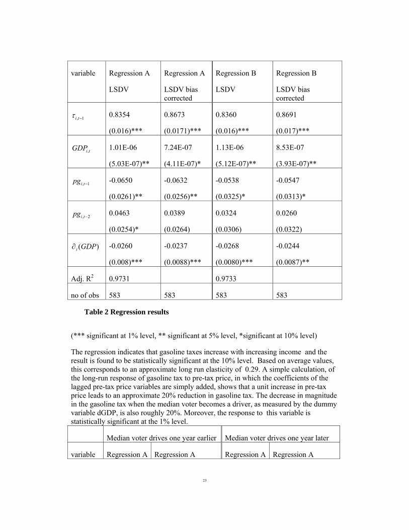
Table 2 Regression results
(*** significant at 1% level, ** significant at 5% level, *significant at 10% level)
The regression indicates that gasoline taxes increase with increasing income and the result is found to be statistically significant at the 10% level. Based on average values, this corresponds to an approximate long run elasticity of 0.29. A simple calculation, of the long-run response of gasoline tax to pre-tax price, in which the coefficients of the lagged pre-tax price variables are simply added, shows that a unit increase in pre-tax price leads to an approximate 20% reduction in gasoline tax. The decrease in magnitude in the gasoline tax when the median voter becomes a driver, as measured by the dummy variable dGDP, is also roughly 20%. Moreover, the response to this variable is statistically significant at the 1% level.
Median voter drives one year earlier Median voter drives one year later
variable Regression A Regression A Regression A Regression A
24
LSDV LSDV bias corrected LSDV LSDV bias corrected
, 1i tτ − 0.8375
(0.0161)***
0.8696
(0.0167)***
0.8425
(0.0159)***
0.8747
(0.0166)***
,i tGDP 7.87E-07
(5.07E-07)
5.06E-07
(4.15E-07)
6.05E-07
(5.05E-07)
3.42E-07
(4.10E-07)
, 1i tpg − -0.0683
(0.0262)***
-0.0662
(0.0258)***
-0.0687
(0.0263)***
-0.0665
(0.0257)***
, 2i tpg − 0.0461
(0.0255)*
0.0386
(0.0264)
0.0441
(0.0256)*
0.0363
(0.0263)
( )i GDP∂ -0.0163
(0.0076)**
-0.0145
(0.0088)
-0.0098
(0.0073)
-0.0090
(0.0089)
Adj. R2 0.9728 0.9726
no of obs 583 583 583 583
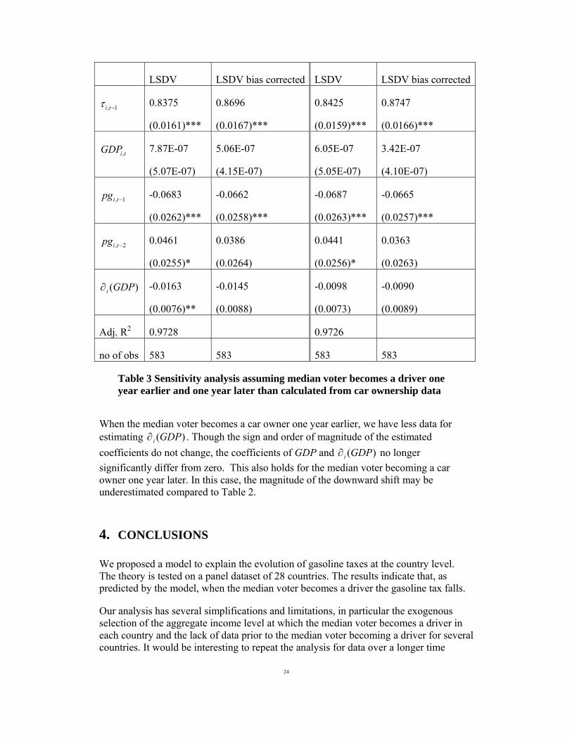
Table 3 Sensitivity analysis assuming median voter becomes a driver one year earlier and one year later than calculated from car ownership data
When the median voter becomes a car owner one year earlier, we have less data for estimating ( )i GDP∂ . Though the sign and order of magnitude of the estimated coefficients do not change, the coefficients of GDP and ( )i GDP∂ no longer significantly differ from zero. This also holds for the median voter becoming a car owner one year later. In this case, the magnitude of the downward shift may be underestimated compared to Table 2.
4. CONCLUSIONS
We proposed a model to explain the evolution of gasoline taxes at the country level. The theory is tested on a panel dataset of 28 countries. The results indicate that, as predicted by the model, when the median voter becomes a driver the gasoline tax falls.
Our analysis has several simplifications and limitations, in particular the exogenous selection of the aggregate income level at which the median voter becomes a driver in each country and the lack of data prior to the median voter becoming a driver for several countries. It would be interesting to repeat the analysis for data over a longer time
25
period, at least for a subset of countries for which data exist. A second extension considered is to test the theory on a more complete cross section and to include road capacity decisions.
26
REFERENCES
Andrews DWK (1993) Tests for parameter instability and structural change with unknown change point. Econometrica, 61, 821-56.
Andrews DWK and Lu B (2001): Consistent model and moment selection procedures for GMM estimation with application to dynamic panel data models. Journal of Econometrics, 101, 123-164.
Bai J and Perron P (1998): Estimating and testing linear models with multiple structural changes. Econometrica, 66, 47-78.
Besley T and Coate S (1997): An economic model of representative democracy. The Quarterly Journal of Economics, 85-114.
Besley TJ and Rosen H (1998): Vertical externalities in tax setting: evidence from gasoline and cigarettes. Journal of Public Economics 70, 383-98.
Bruno, GSF (2005):. Approximating the bias of the LSDV estimator for dynamic unbalanced panel data models. Economics Letters, 87, 361-366.
Bruno GSF, Anna M. Falzoni AM and Helg R(2004): Measuring the effect of globalization on labour demand elasticity: An empirical application to OECD countries, CESPRI Working Paper n153.
Bun MJG and Carree MJ (2006): Bias-corrected estimation in dynamic panel data models with heteroscedasticity. Economic Letters, 92, 220-227
Bun MJG and Kiviet JF (2003): On the diminishing returns of higher-order terms in asymptotic expansions of bias. Economic Letters, 79, 145-152.
Bun MJG and Kiviet JF (2006): The effects of dynamic feedbacks on LS and MM estimator accuracy in panel data models. Journal of Econometrics, 132, 409-444.
de Wachter S and Tzavalis E (2004): Detection of structural breaks in linear dynamic panel data models. Department of Economics, Queen Mary University of London Working Paper No. 505.
Downs A (1957): An economic theory of democracy. Harper and Row, NY.
Decker CS and Wohar ME (2007): Determinants of state diesel fuel tax rates: the political economy of fuel taxation in the United States. Annals of Regional Science, 41, 171-188.
Fredriksson PG and Millimet D (2004): Comparative politics and environmental taxation. Journal of Environmental Economics and Management, 48, 705-722.
Gevers L, Proost S (1978): Some effects of taxation and collective goods in postwar America – a tentative appraisal. Journal of Public Economics, 9, 115-137.
27
Glazer A and Proost S (2007): The preferences of voters over road tolls and road capacity. CES Discussion paper series, 07.09, KU Leuven. (http://www.econ.kuleuven.be/ces/discussionpapers/Dps07/Dps0709.pdf)
Goel RK and Nelson MA (1999): The political economy of motor fuel taxation. The Energy Journal, 20, 43-59.
Hammar H, Loefgren A and Sterner T (2004): Political economy obstacle to fuel taxation. The Energy Journal,25, 2-17.
Hsing Y (1994): Estimating the impact of the higher fuel tax on US gasoline consumption and policy implications. Applied Economics Letters, 1, 4-7.
IEA (1998): Energy Prices and Statistics- Quarterly Statistics (Fourth Quarter).
IEA (2006): Energy Prices and Statistics- Quarterly Statistics (Second Quarter).
Jochimsen B and Nuscheler R (2005): The political economy of the German länder deficits. Unpublished Working Paper.
Judson RA and Owen AL (1999): Estimating dynamic panel data models: a guide for macroeconomists. Economic Letters, 65, 9-15.
Mohn K and Misund B (2009): Investment and uncertainty in the international oil and gas industry. Energy Economics, 31, 240-248,
Obfsgård A and Zahran Z (2008): Corruption and political and economic reforms: A structural breaks approach. Economics and Politics, 20, 156-184.
OECD Factbook 2008: Economic, Environmental and Social Statistics.
Persson, T. Tabellini, G. (1999), The size and scope of government: comparative politics with rational politicians, European Economic Review, 43(4-6), 699-735
Persson T, Roland G and Tabellini (1997): Separation of powers and political accountability. Quarterly Journal of Economics, 112, 1163–1202.
Philips PCB and Sul D (2007): Bias in dynamic panel estimation with fixed effects, incidental trends and cross section dependence. Journal of Econometrics, 137, 162-188.
Pock M (2007): Gasoline and Diesel Demand in Europe: New Insights. Economic Series 2002, Institute for Advance Studies, Vienna.
Rietveld P and van Woudenberg S (2005): Why fuel prices differ. Energy Economics, 27, 79-92.
Romer H and Rosenthal T (1979): The elusive median voter. Journal of Public Economics, 12, 143-170.
28
Small K and Verhoef E (2007): The economics of urban transportation. Routledge.
Wooldridge, J. M. JM (2002): Econometric Analysis of Cross Section and Panel Data. Cambridge, MA, MIT Press.
29
APPENDIX 1
0.3
0.4
0.5
0.6
0.7
0.8
0.9
1
10000 15000 20000 25000 30000 35000
GDP/cap
real
tax
Austria
Belgium
Germany
Switzerland
Luxembourg
Netherlands
Figure A1 Observed real gasoline taxes versus GDP per capita for selected European countries (US dollars in year 2000 prices)
30
0
0.1
0.2
0.3
0.4
0.5
0.6
0.7
0.8
10000 15000 20000 25000 30000 35000
GDP/cap
real
tax
Canada
Japan
New Zealand
USA
Figure A2 Observed real gasoline taxes versus GDP per capita for low tax regime countries (US dollars in year 2000 prices)
31
0
0.5
1
1.5
2
2.5
3
3.5
4
10000 15000 20000 25000
GDP/cap
real
tax
The Czech Republic
Hungary
Poland
Slovakia
Figure A3 Observed real gasoline taxes versus GDP per capita for new member European countries (US dollars in year 2000 prices)