October, 2006 What drives Provincial – Canada Yield Spreads? Laurence Booth, 1 George Georgopoulos 2 and Walid Hejazi 1 (1) Rotman School of Management, University of Toronto (2) Economics, Atkinson Faculty of Liberal and Professional Studies, York University Abstract Although recent research has led to a deeper understanding of the factors determining yields on long term Canada bonds, there has been little corresponding work on provincial bonds. This is despite the fact that unlike the US state bond market, provincial debt represents a significant part of the Canadian bond market. Provincial and state debt are examples of sub-national debt which are backed by taxing powers similar to that of the national government, but without control of the money supply, which leaves them open to the possibility of default or payment rescheduling. This in turn makes them similar to corporate debt. By using a carefully constructed new data set we establish two important results. First, provincial fiscal positions (debt and deficits) are an important factor in determining yield spreads between provincial and Canada bonds. Second we show that provincial bonds are a substitute for corporate debt, in that during recessionary “flights to quality” their yields react similar to those on corporate bonds. Keywords: Interest Rates, Provincial GDP JEL Classification: E43, E44 Correspondence to: Walid Hejazi, Rotman School Management, University of Toronto, 105 St. George St., Toronto, Ontario, Canada, M5S 3E6. [email protected]
Transcript
October, 2006
What drives Provincial – Canada Yield Spreads?
Laurence Booth,1 George Georgopoulos2 and Walid Hejazi1 (1) Rotman School of Management, University of Toronto (2) Economics, Atkinson Faculty of Liberal and Professional Studies, York University
Abstract
Although recent research has led to a deeper understanding of the factors determining yields on long term Canada bonds, there has been little corresponding work on provincial bonds. This is despite the fact that unlike the US state bond market, provincial debt represents a significant part of the Canadian bond market. Provincial and state debt are examples of sub-national debt which are backed by taxing powers similar to that of the national government, but without control of the money supply, which leaves them open to the possibility of default or payment rescheduling. This in turn makes them similar to corporate debt. By using a carefully constructed new data set we establish two important results. First, provincial fiscal positions (debt and deficits) are an important factor in determining yield spreads between provincial and Canada bonds. Second we show that provincial bonds are a substitute for corporate debt, in that during recessionary “flights to quality” their yields react similar to those on corporate bonds.
Keywords: Interest Rates, Provincial GDP JEL Classification: E43, E44
Correspondence to: Walid Hejazi, Rotman School Management, University of Toronto, 105 St. George St., Toronto, Ontario, Canada, M5S 3E6. [email protected]
1
1. Introduction
Canada is a federation with strong federal and provincial governments and shared responsibilities.
The federal government is the national government and we will refer to provincial governments as
sub-national governments. Within Canada program spending by the provinces is about 30%
greater than that of the federal government, while the province of Ontario alone spends almost half
as much as the Federal government.1 This spending is economically significant, as are the
implications for financial markets where 35% of the Canadian bond market consists of provincial
bonds. Yet while there has been significant research into the factors that determine the yields on
long-term Canada bonds (Booth (1995), Boothe (1991), Gauthier et al. (2004), Hejazi, Marr and
Parkinson (2000) and Johnson (1993)), there has been relatively little research into the factors
determining provincial bond yields. This research will examine whether the impact of provincial
debt and deficits affect their yield spreads over equivalent term Canada bonds, which we will refer
to generically as the provincial spread.
Whether debt and deficits affect long term interest rates remains a controversial question for
national debt, let alone sub-national debt. In a recent review Friedman (2005) states “A long
history of efforts to establish an empirical relationship between observed deficits and observed
interest rates – has generated widely varying estimates.” Most macro-economic models would
predict a short run impact of deficit spending on long term interest rates due to changes in
aggregate demand and short run stickiness in the economy. However, Barro (1974) argued that
Ricardian equivalence would generate offsetting savings by investor-taxpayers who explicitly
recognize that increases in government debt imply higher future tax payments. Consequently, they
save more to generate the interest receipts necessary to make the future tax payments, thereby
negating the impact of deficit financing on aggregate demand. Whether investor-tax payers are as
omniscient as implied by Barro has not been conclusively proved either way, so that it is an
empirical question as to whether debt and deficits affect interest rates.
However, for provincial bonds there is an additional effect of deficits and the supply of
1. As of 2004 program spending by the Government of Canada was $158 billion and that of Ontario $70 billion, with total provincial program spending of $202 billion.
2
sub-national debt, which is increased liquidity. Amihud and Mendelson (1991) showed that even
in the US bond market differences in liquidity for otherwise similar US government bonds
generated significant yield spreads. Consequently, the observation of positive provincial yield
spreads could simply reflect the greater liquidity of Government of Canada bonds. In this case,
increased supply of provincial bonds may increase their liquidity, making them better substitutes
for Government of Canada bonds and causing their spreads to decrease.
This tension between the two opposite effects of an increasing supply of provincial bonds means
that it is an empirical question as to how provincial spreads are affected by debt and deficits. In this
paper we look at the empirical evidence by using a carefully constructed new data base of
provincial bond yield spreads over equivalent term long Canada bonds. As far as we are aware
no-one has ever looked at the yield spreads of sub-national debt either in Canada or the United
States. Instead, research has relied on bond ratings with the drawback that they do not reflect
contemporaneous market forces because they are sticky, in the sense that the “stable rating”
philosophy adopted by rating agencies makes them reluctant to make frequent changes to ratings.
Our research is not be subject to this criticism.
This research also has implications for the emergence of regional blocks on the global stage, such
as the European Monetary Union. The implications of sub-national economic policy making
within a national government context is becoming increasingly important, and yet has not been
subject to significant research. This paper works to fill this void.
The outline of the paper is as follows. Section 2 considers the existing literature and competing
hypotheses as to the effect of government debt and deficits on interest rates and liquidity. Section
3 reviews some of the main institutional features of the Canadian bond market and recent trends to
provide some perspective. Section 4 discusses the data, hypotheses and empirical specifications.
Section 5 discusses the empirical results and Section 6 provides our conclusions.
2. Factors Affecting the Yield Spread
Following Bernoth et al. (2004) assume an investor has a mean variance utility function (U)
3
expressed over terminal income (Y) and for convenience makes myopic2 single period investment
decisions, such that the utility function can be expressed as
))](([ αα
YUEMaxU=
where the choice variable is the proportion of wealth (α) invested in provincial bonds. The investor
can either invest (α) in provincial bonds (P) or (1-α) in the benchmark Canada bond (C). The
Government of Canada bond is the benchmark bond since it is default free and completely liquid
in normal trading volumes with a stated interest rate of r. In comparison the provincial bond has a
promised rate of return R, but has a probability of default (π) in which case the payoff is β% of the
par value. If the bond does not default then the payoff is (1+R) with probability (1-π). In either
case there are liquidity or trading costs on the provincial bond of γ.
The expected terminal wealth is
])1)(1())1)(1(([)( αγαππβαα −+−++−+= rRWY
This is simply the portfolio weighted average of the probability weighted payoff from the
provincial bond and the Canada bond. Since the payoff from the Canada bond and the transaction
cost on the provincial bond are risk-free, the variance of the uncertain payoff from the two possible
states of nature is simply
222 )1)(1()( βππα −+−= RWYVar
The first order optimality condition is
0)])1()1)(1()(([ ' =−+−+−+ γππβ rRYUE
Solving for the optimal investment proportion (α) gives
2. See Mossin (1969) for a discussion of the conditions under which multi-period investment decisions can be collapsed into a single period decision in a discrete time framework. In a continuous time framework the conditions are less onerous, but their development would detract from the objective of this research.
4
2
1
)1)(1())1()1)(1((
βππγππβθ
α−+−
−+−+−+=
−
RrRi (1)
where
)]([)]([
'
''
YUEWYUE
i =θ
is a measure of the investor’s relative risk aversion and its inverse the investor’s risk tolerance.
The optimality condition is the standard mean variance condition, where the optimal investment
proportions are the expected risk premium divided by the variance of the investment weighted by
the investor’s risk aversion.
If we multiply (1) by each investor’s wealth to get the demand for the provincial bond, equilibrium
in the bond market requires that supply equals demand, and rearranging we get the yield spread
12)1)(1()1( −−+−++−+=− φβππγβπ RSRrR (2)
where
∑=
−−=n
iii W
1
11 )( θφ
is the market’s risk tolerance weighted wealth, which reflects the importance of each investor’s
risk tolerance in determining market prices and S is the supply of provincial debt. As a result, the
spread between the provincial and Canada bond is determined by three basic factors.
Consider the third factor first, which is the risk premium. If investors are risk neutral then their risk
tolerance becomes infinite and the inverse of the market’s risk tolerance in (2) drives the third term
to zero, that is, there is no risk premium. In this case the provincial bond yield is higher than the
Canada bond yield due to the second term, which is the higher transaction/liquidity cost attached
to the provincial bond, and the first term which is the loss in value from the possibility of a
rescheduling of the provincial bond’s cash flows. On an expected value basis, even without risk
5
aversion, the investor requires a higher yield from the provincial bond to reflect the cash flow loss
from this potential rescheduling. What (2) shows is that conceptually the yield spread consists of
three factors. However, there are questions as to whether they all exist.
The existence of a risk premium depends on whether tax revenues can be raised to make interest
payments, which in turn depends on whether Ricardian equivalence (Barro 1974) holds at a
sub-national government level. If investor-tax payers consolidate per capita provincial balance
sheets with their own and recognize the higher future tax payments as provincial debt increases,
then investor-tax payer saving rates will adjust for the provincial saving rate (borrowing). Barro’s
argument for the irrelevance of national debt applies equally to provincial debt, since it relies on
the tax raising ability of the government, rather than control of the money supply. It also means
that in equilibrium, since we owe the provincial debt to ourselves, the supply of provincial debt is
equal to zero and the risk premium, disappears.3
However, Ricardian equivalence also depends on whether investor-taxpayers are immobile.4
Otherwise, investor-taxpayers can simply consume the extra resources provided by increased
government spending and move before paying the higher tax bill. In this context Sillimaa and
Olson (2003) examine administrative data for 2 million tax filers kept by Statistics Canada. They
find that over the period 1985 to 1989, a 1 percentage point increase in the marginal tax rate
resulted in the movement of about 300 new prime-aged adult migrants per year. However, in the
face of tax differences across the provinces, that currently range from a low of 39% for Alberta to
a high of 48.6% in Newfoundland, this still implies relatively low labour mobility. Similarly, for
the US, evidence by Kotlikoff and Raffelhueschen (1991) indicates that “regional fiscal
differences play an important role in the location choices of three to four percent of Americans.”
Whether this indication of relative labor immobility is sufficient to offset the Barro argument or
not is an empirical question.
Most policy makers believe in a positive relationship between interest rates and government debt
and deficit levels, which by implication translates into higher provincial spreads for increasing
3. Default risk may also be diversifiable in a more detailed portfolio balance model. 4. Ricardian equivalence requires some additional conditions, including infinite lives and no borrowing constraints.
6
supplies of provincial debt. Paul Martin when Canadian Finance Minister, for example, stated
(1996, p 207) “endless deficits really did have something to do with Canada’s high real interest
rates, and that higher government spending really did translate into higher taxes, the tolerance for
which had reached its limit.”5 However, the empirical evidence is ambiguous. The early work of
Plosser (1982 and 1987) and Evans (1985 and 1987a,b) using U.S. data and Siklos (1988) using
Canadian data generally found no direct link between government deficits and interest rates. One
possible reason for these results is the estimation period. Plosser’s work, for example, covers the
period 1954-1978 when government deficits were not as serious as they subsequently became.
More recent empirical work, for example, Nunes-Correia and Stemitsiotis (1993) find that deficits
affect interest rates, where they estimate a 1% increase in the deficit increases real interest rates by
0.53%. Similarly, Booth (1995) estimates a 0.26% increase, and using a VECM approach Gauthier
et al. (2004) estimate an even stronger result where a 0.2% increase in the deficit increases
nominal long term interest rates by 0.40%. Ardagna et al. (2005) most recently used a panel of 12
OECD countries and estimated that a 1.0% increase in the debt to GDP ratio led to a
contemporaneous increase in long term interest rates of 10 basis points increasing to 150 basis
points after ten years.
Apart from default risk, provincial spreads are also affected by low liquidity induced transaction
costs. Van Horne (1978) describes liquidity as the “ability to realize value in money.” It has two
main dimensions: the cost of transacting, and the volume that can be transacted, both of which are
important for financial markets. Amihud and Mendelson (1991) examined the impact of liquidity
in the largest most liquid bond market in the world, that for U.S. Government bonds. They pointed
out that the bid-ask spread for a US$1 million transaction in Treasury Bills was 1/128th of a point
plus a brokerage fee of $12.5-$25 per million. In contrast, a similar sized transaction in Treasury
Notes had a 1/32 spread plus a brokerage fee of $78.125 per million. The discounted value of these
differential transactions cost streams is then impounded in market prices to cause liquidity spreads
between different US government securities, where there is no default or rescheduling risk.
If liquidity differences can cause spreads between otherwise similar US government bonds, then it 5. Interestingly the Martin quotation that taxes have “reached a limit” is echoed in Barro, where he notes “The amount of bond issue would be limited by the government’s collateral, in the sense of its taxing
7
is natural to expect the size differences in outstanding debt issues between the government of
Canada and the provinces to cause differential liquidity spreads. In this case, increased supply of
provincial bonds will reduce liquidity spreads causing the differences between Canada and
provincial bonds to narrow. Further, we would expect two provinces with the same debt and deficit
problems, relative to GDP, to have different spreads if the absolute size of their bond markets, and
thus their liquidity, is different.
Surprisingly there has been very little work on provincial or sub-national bond markets. Mattina
and Delorme (1997) looked at the impact of fiscal policy on the provincial spreads for Ontario,
Quebec, British Columbia and Nova Scotia bonds. Using British Columbia as a benchmark, they
estimated a non-linear supply curve. Bayoumi, Goldstein and Woglom (BGW 1995) used survey
data on 20-year general obligation US state bonds and also found evidence for a non-linear supply
curve.6 The BGW study was motivated by the same concerns as our paper that the US state
experience as sub-national units in a monetary union may have implications for countries that are
now part of the European Union with a common currency. In a similar vein, Alesina et al. (1992)
for a sample of 12 OECD countries found a strong correlation between the size of public debt
markets and spreads between public and private rates of return. Moreover Bernoth et al. (2004) in
a recent European Central Bank working paper find that the spreads on bonds of countries within
the European Union over German and US bonds reflect positive default and liquidity effects.
However, as far as we are aware no-one has looked at this tension between the liquidity and
rescheduling effects of the supply of provincial bonds. Whether debt and deficits cause portfolio
balance effects in requiring higher yields to induce investors to hold them or lower yields since
they look more like Canada bonds is an open empirical question.
capacity to finance the interest and principal payments.” 6. U.S. state and local bonds, also called municipal bonds, are long term instruments issued by state and local governments to finance expenditures on schools, roads, and other large regional programs. The interest payments on these bonds are exempt from federal income tax and generally from state taxes in the issuing state. The largest buyers of these securities are commercial banks, who, with their high income tax rate, own over half of the total bonds outstanding. The next biggest group of holders is wealthy individuals also with high income tax brackets, followed by insurance companies.
8
3. Canadian Bond Market
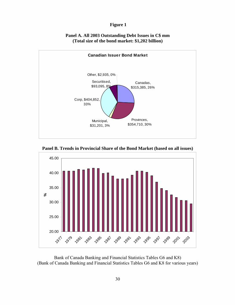
Figure 1 Panel A indicates that in 2003 fully 30% of the $1,202 billion Canadian bond market
consisted of debt issued or unconditionally guaranteed by the provinces. The other major issuers
are the Canadian government (Canadas) with 26%, the corporate sector with 33% and specialised
securitisations with 8%. This latter amount consists of pass-throughs of mortgages and other
bonds backed by loans, credit card receivables, etc. The residual consists of the municipal bond
sector and some foreign issuers in Canada. Panel B shows the trend in the provincial share over the
last 26 years. Traditionally provincial bonds have been about 40% of the overall bond market.
However, the provincial share started to decline in 1993 as all levels of government focussed on
deficit reduction and corporate bond issues increased. Since 1997 the provincial share has
experienced a persistent downward trend.
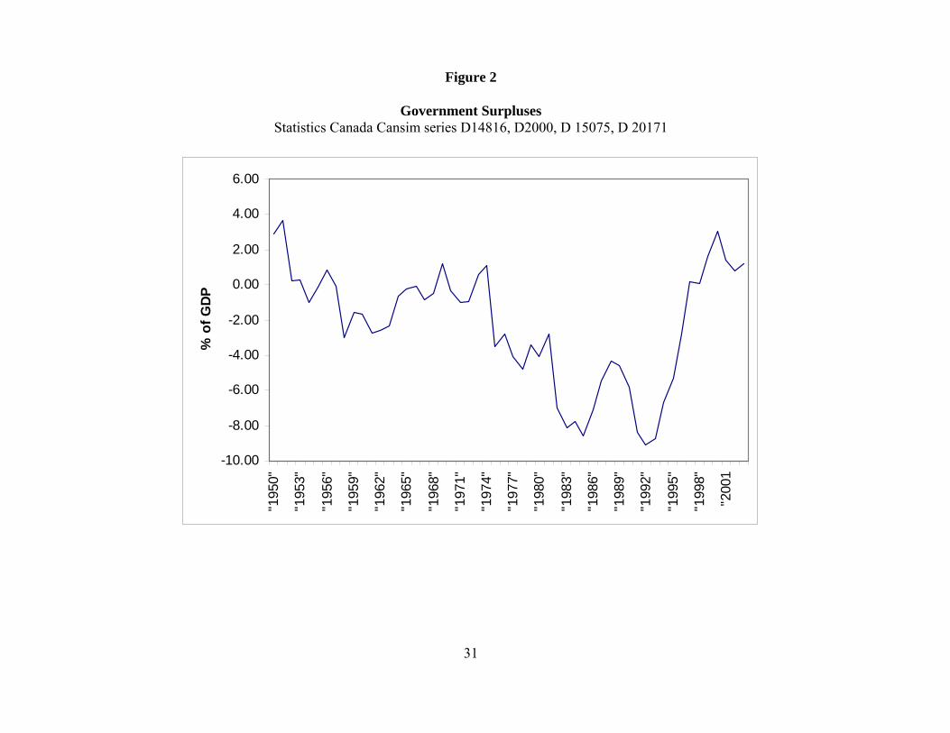
The importance of the government segment of the bond market is simply the mirror image of
government deficit problems. Figure 2 indicates the aggregate Canadian government deficit, both
federal and provincial, as a percentage of GDP. The deficit was around zero until the late 1970s
when it started to increase significantly and reached cyclical lows in the recessions of the early
1980s and 1990s at -8.2% of GDP in 1983 and -9.13% in 1992. After 1993 the deficit was reduced
almost yearly until it achieved a peak surplus of over 3.0% of GDP in 2000, before softening with
the slowdown in the early 2000s. However, in contrast with other G-8 countries the Canadian
government in aggregate remains in surplus. One implication of the data in Figure 2 is that the
early tests on Canadian data prior to the late 1970s covered a period when deficit problems were
not as acute as they subsequently became.
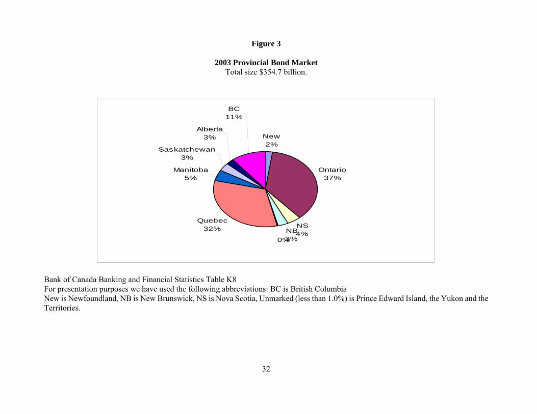
Figure 3 shows the composition of the provincial bond market for 2003. Overall the provincial
bond market was worth $354.7 billion. Quebec, Ontario and BC account for 80% of this total. The
rest are scattered at 3-4% levels each except for Prince Edward Island and the Territories, which
together account for less than 1.0%. However, even though 4% seems like a small number, for
2003 this amounted to $16.5 billion for Manitoba, which dwarfs almost all corporate issuers and
may indicate significant liquidity differences between provincial and corporate debt.7
7. Government borrowing is from a variety of sources, but the use of non-market sources such as the Canada
9
Table 1 provides data on the liquidity of the bond market, where liquidity is defined as the turnover
or the average monthly trading volume divided by the stock of outstanding debt. Canada bonds are
overwhelmingly the most liquid, where on average there is a 20-30% turnover a year. In contrast
there is just a 1.4% turnover in the corporate bond market and about a 2.5% in provincial bonds.
The liquidity data reflects the heterogeneity of the corporate bond market, the homogeneity of the
Canada segment, with the provincial segment in between.8 The data also indicates that investors in
non-Canada bonds partially give up the right to trade these bonds given their evident lack of
liquidity. However, this lack of liquidity varies from province to province. Ontario and Quebec
typically re-enter existing issues to build liquidity in their own benchmark bonds. This also
facilitates stripping and subsequent reconstituting of their bonds, which again enhances their
liquidity.9 However, the smaller provinces usually sell their bonds on a “one off” basis as bought
deals so their issues tend to be small and lack liquidity similar to corporate bonds.
Before formally testing specific hypotheses, consider the behaviour of corporate spreads.
Corporate bonds are both less liquid and more default risky than provincial bonds. Consequently
we would expect them to be sensitive to the business cycle consistent with Atkinson’s (1967)
original results. This is what Figure 4 shows, where the spreads are those between BBB rated
corporate bonds and equivalent maturity long Canada bonds. The spreads are clearly inversely
related to corporate profitability, as measured by Statistics Canada as the average return on equity
(ROE) for “Corporate Canada.”
If corporate spreads are sensitive to the business cycle what about provincial spreads? Figure 5
plots the spreads on the long term Provincial and Corporate bond indexes maintained by Scotia
Pension Plan (CPP), and the Ontario Teachers Pension Fund has dropped dramatically since the late 1980s, as both have been freed from the requirement to buy government debt. 8. The public good aspect of the Canada bond market is taken seriously by the Government of Canada, which has taken significant steps to preserve the liquidity of the benchmark bonds. For example, when the Government of Canada decreased the frequency of Canada bond auctions from quarterly to semi-annually in April 1998, it also shifted its financing from Treasury Bills to long Canada bonds and repurchased illiquid off the run bonds. 9. Stripping bonds simply means selling off individual coupons. Once this is done it only used to be possible to reconstitute the bond by buying back all the original pieces. The movement to common terms and coupons for the benchmark bonds and the use of generic identifiers makes it easier to reconstitute the bonds and arbitrage.
10
Capital over similar maturity Canada bonds back to 1977.10 The spreads are based on index data
and so reflect a weighted average of provincial and corporate issuers. The provincial spread is
usually lower than the corporate spread, due possibly to the greater liquidity discussed earlier, and
lower default risk. More importantly, the recession and slow downs of the early 1980s, 1990s and
2000s is clearly evident in wider spreads for both corporate and provincial issuers, although the
impact on corporate issuers is more attenuated.11 The casual empiricism of Figures 4 and 5
indicates that provincial and corporate bonds seem to be substitutes in responding in a similar
fashion to broad macro-economic effects. However, the graphs say little about the role of debt and
deficits in determining these spreads except that the provincial spreads have been lower than the
equivalent corporate spreads since about 1997, when government deficits from Figure 2 moved
into surpluses.
4. Data and Hypotheses
To examine the impact of debt and deficits on provincial yield spreads we hand collected monthly
yield data on long-term provincial government bonds for the period 1981 to the end of 2000 from
the Financial Post.12 The yields were calculated as follows: an average was estimated for all bonds
outstanding for each province with a maturity of 5 to 10 years, weighted by the amount of bonds
outstanding for that maturity. This was done for each province, from 1981:1 to 2000:12. There
were no data available for Prince Edward Island (PEI) for the last nine months of 2000 or for
British Columbia for the period 1981:1 to 1983:8. Yields on Canadian benchmark bonds were
obtained from CANSIM. The yield data reflected transaction yields, except for some of the smaller
issues, where they were indicative yield quotes by investment dealers making a market in the
bonds. In this latter case they still reflect market conditions since providing stale quotes would
10. Equivalent BBB and ROE data is not available this far back. The Scotia Capital Indexes are the standard benchmarks for Canadian yield data and are used in the Bank of Canada Review. 11. Different econometric modeling of the provincial against the corporate spread indicates that it varies by 56-65% of the corporate spread. 12. Time series data on provincial bonds is difficult to obtain. The only publicly available data is that for the overall provincial bond index which is maintained by Scotia Capital. Landon and Smith (2000) in their study of spill over effects in the Canadian bond market justify their use of bond ratings as their dependent variable on the grounds that comparable yield data is not available. Bayoumi et al. (1995) rely on semi-annual surveys of municipal bond traders to retrieve the yield data used in their analysis of the US bond market.
11
soon drive an investment dealer out of business.13
Table 2 provides descriptive statistics for our interest rate data. The average yield on medium term
Canadas was 8.47%. The province with the highest average yield was Prince Edward Island at
9.54%, followed by Newfoundland at 9.49%. The province with the lowest average yield was
Alberta at 8.89%. The next four lowest provincial yields are very close to one another with Ontario
at 9.09%, British Columbia at 9.11%, and Manitoba and Saskatchewan each at 9.12%. Over this
period the average yield curve was normal as long Canada bonds yielded 0.33% over medium term
Canada bonds, and mediums 0.96% over short term Canadas.
Of interest are the yield spreads in Table 2, where consistent with the average yield data described
above, the average spread runs from a low for Alberta of 0.13% to a high for Newfoundland of
0.71% or 71 basis points. In all cases the maximum spread occurred either in the recession of the
early 1980s or that of the early 1990s. It is worth noting that on several occasions, the spread for
Alberta was negative, that is, the yield on Alberta provincial bonds was lower than that for Canada.
This should not be entirely surprising given that Alberta has run surpluses over much of this time
period. In addition, the Alberta government maintains the Heritage Fund of several billion dollars
which is derived from its provincial revenue and is actively paying down its provincial debt. The
summary data indicates that there is significant dispersion in the provincial spreads, so there is
something to explain.
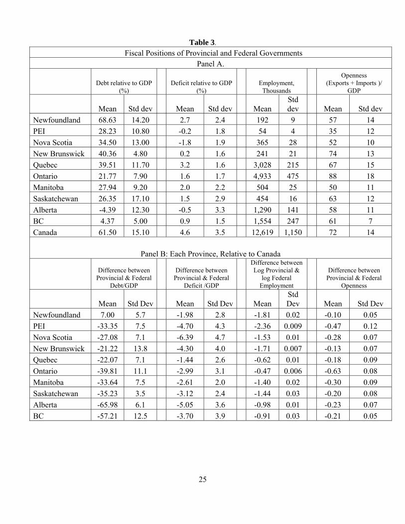
For our independent variables we hypothesize that the probability of default or rescheduling is
determined by the following provincial values relative to Canada: total debt, annual budget deficit,
employment, and openness variables (discussed in detail below). Descriptive statistics for these
values are in Table 3, where Panel A provides the data for each province and Canada and Panel B
the difference variables we use to estimate the model.
The debt levels come from the Financial Management System, which expresses all the provincial
budgets on a consistent basis and includes provincial assets as well as marketable and
non-marketable debt. Consequently the level of indebtedness is a broader and more encompassing
13. New issue yields are unreliable simply because of the lack of a continuous time series for most provinces.
12
measure than simply the amount of public market bonds outstanding. The average debt load varies
from -4.39% of GDP for Alberta to 68.6% for Newfoundland. The negative debt for Alberta
indicates that provincial assets exceeded liabilities, in this case due to the Heritage fund and the oil
and gas royalties earned by the province.
There is also wide variation in the deficit levels across provinces. For the deficit variable a
negative value denotes a surplus and a positive value a deficit. All provinces have run deficits at
various times. The highest deficits have split evenly in both the 1980s and 1990s with five
provinces recording their highest deficit in the 1980s and five in the 1990s. Overall, provincial
deficits have not been as significant as those of the Government of Canada, but the data indicate
significant dispersion both across time and across provinces.
We used employment and openness variables as provincial characteristics to capture other effects
that might affect the rescheduling risk, as well as dummy variables for specific political events that
likely influenced spreads. The employment data is meant to indicate trends in income tax revenues
and the ability of a province to increase taxes. The conjecture is that employment levels indicate
a private wealth effect independent of the impact on the provincial deficit: the higher the level of
employment the higher the level of savings and investment. The trade data is an openness index
defined as the sum of exports and imports divided by provincial GDP. This latter variable has been
used extensively in sovereign debt research to gauge the ability of a country to generate hard
currency. In our case it indicates the ability of a province to attract international business and we
use it as a broad measure of awareness and competitiveness.
In addition to these four characteristic variables for each province, we also used dummy variables
for five significant political events. Since political uncertainty surrounding potential Quebec
separation is known to have affected Canadian Treasury bill and bond yields (Hejazi, Marr and
Parkinson (2000), Johnson and McIlraith (1998), Shum (1995)), we therefore test whether they
also impacted provincial spreads.
In the discussion of prior research we noted that several researchers had found non-linear effects.
We might expect this if there is a tipping point in terms of the impact of debt and deficits. To
account for this we use an extreme variable which indicates a situation where everything is “going
13
bad” with higher deficit levels compounding the effects of higher debt levels. The extreme
variable is designed to capture the intuition that the effect of a higher deficit is greater when the
existing debt load is also high. It thus implicitly incorporates non-linearities in the supply of
provincial debt. The extreme variable is one if both the province and Canada have debt and deficit
levels above their average level, and zero otherwise.
The above discussion leads to the following estimating equation,
where i denotes province (i = 1,…10) and t denotes tine in quarters (t = 1981Q1, …, 2000 Q4). The
variables are defined as follows:
• Spread is the provincial yield spread over the equivalent Canada bond. • debt is the difference between the provincial debt to GDP ratio and that of the
Government of Canada. Differences were used since some of the provincial debt ratios are negative indicating surpluses.
• deficit is the difference between the provincial deficit as a percentage of provincial GDP and the same for Canada, and again differences are used since some of the deficits are negative (surpluses).
• employ is the difference between the natural logarithm of provincial level employment and the natural log of Canada level employment.
• open is the difference between the natural logarithm of the sum of provincial exports and imports to GDP and that for Canada.
• extreme is a dummy variable that captures above average values to debt and deficits for both Canada and the provinces. This variable takes on a value of one when both the provincial and Canada debt and deficits relative to GDP are simultaneously above average, and zero otherwise.
• political is a dummy variable which captures the impact of known periods of political uncertainty. This variable takes on a value of one when during periods of political uncertainty discussed below, and zero otherwise.
If fiscal imbalances and levels of government debt do not impact yields, then β1=β2=0. If debt and
deficits cause increased liquidity then β1, β2<0. Alternatively if increased debt and deficits
increase rescheduling concerns β1, β2>0. We hypothesize that increased employment generates a
wealth effect and lower spreads either through increased demand for provincial securities or lower
rescheduling risk β3 <0. We argue that the greater the international linkages of a province the more
14
competitive it is, so β4< 0.
There have been several political events surrounding the possible separation of Quebec from
Canada. These events are:
* 1990 Quarter 2: Failure of the Meech Lake Accord * 1992 Quarter 3: Charlottetown Accord defeated on October 1992 * 1995 Quarter 3: 2nd Quebec referendum announced August 1995
* 1995 Quarter 4: October 30 Quebec referendum
Dummy variables were used to reflect these four specific events as the associated uncertainty is
known to have affected Canadian bond yields, and hence provincial spreads. Our political dummy
variable takes on a value of one in these periods, and zero otherwise. Although the provincial yield
data are available monthly, provincial GDP is only available quarterly. Hence we use quarterly
data for 1981 to 2000.
5. Empirical Results
We test for the presence of non-stationarity in each of the variables used in the model. These tests
are undertaken in a panel framework using the Fisher panel unit root test methodology, where the
null hypothesis is non-stationarity. We find that all but two variables are non-stationary, those two
being the spread and the deficit.14 Given the existence of non-stationary variables we estimated the
Pedroni (1995) panel co-integration test, where the null is no co-integration in heterogeneous
panels with multiple regressors.15 Pedroni derives two residual based test statistics that are
analogous to the Phillips–Perron and augmented Dickey –Fuller t-statistics. The panel
co-integration Phillips-Peron test statistic for the variables spread, debt, deficit, employ, open, is
-11.32, and the augmented Dickey-Fuller statistic is -4.38. Both statistics allow us to reject the null
of no co-integration at the 1% level of significance. In other words, this multivariate panel
co-integration regression test finds that our variables are co-integrated.
14. The Fisher test combines the p-values from n independent unit root tests, as developed by Maddala and Wu (1999). The panel unit root p values for the spread, debt/gdp differences, deficit/gdp differences, employment differences, openness differences are 0.001, 0.255, 0.938, 0.0428, 0.999 respectively. 15. Pedroni shows that these are one-sided tests with standard normal test statistics as both the time series and cross-sectional dimensions of the panel grow large.
15
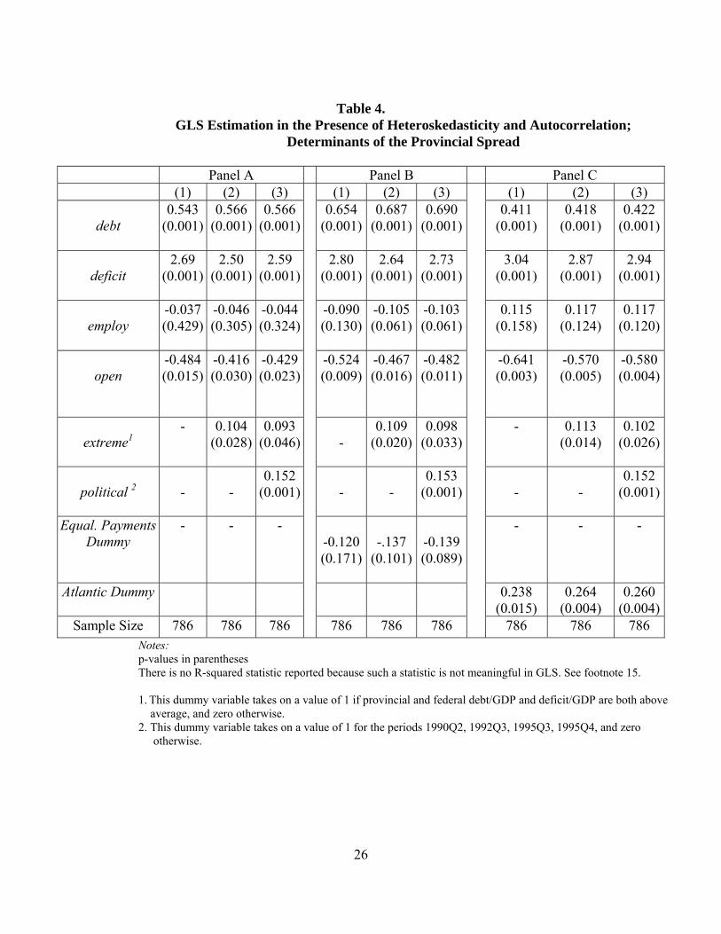
Our initial OLS estimates of our model tested for panel level heteroskedasticity and
autocorrelation (Woolridge 2002), where the test statistics for both tests rejected the null of no
heteroskedasticity and no autocorrelation. Consequently we estimated our model using feasible
GLS which allows for autocorrelation and heteroskedasticity across panels. These results are
presented in Panel A. Three of the four independent variables are significant, indicating that both
the size of the debt and the deficit relative to that of the Government of Canada tends to increase
provincial yield spreads.
Note from Tables 2 and 3, the spreads, debt and deficit data are all in percentages, so the empirical
results indicate that a 1% increase in provincial debt to GDP relative to Canada increases the
spread by 0.54 basis points. To put this in perspective if the debt to GDP ranges between 20% and
50%, all else constant the provincial spread would range between 11-27 basis points. Similarly, if
the deficit to GDP ranges between 5.0% and 10.0%, all else constant the spread would range
between 14-26 basis points. The fact that the signs on both the debt and deficit variables are
significantly positive indicates that the risk effect of provincial debt outweighs any liquidity effect.
The ratio of provincial-federal employment difference indicates that increasing provincial
employment levels reduce the provincial spread, but the coefficient is not significant.
Interestingly, the negative and significant sign on the openness variable confirms the hypothesis
of lower risk associated with provinces that are relatively more diversified through high levels of
international integration.
The models in columns 2 and 3 repeat the tests with the added “extreme” value variable and the
political dummies. Interestingly, while the coefficients on the independent variables are largely
unchanged, the impact of the extreme variable indicates an extra 10 basis points is added to the
provincial spread, whereas the four political events seem to have added another 15 basis points.
Clearly there are some non-linearities in the impact of debt and deficits on provincial spreads, and
as you would expect, political events affect the attractiveness of holding provincial bonds and thus
their spreads. Again the sign and significance of the debt and deficit variables indicate that spreads
are primarily affected by risk rather than liquidity concerns.
There are two other factors that we considered. Canada has some provinces that consistently
16
receive equalization payments from the federal government. These transfer payments represent
another source of revenue to the provincial governments and hence may affect spreads. At the
same time there are size differences across the provinces with the four Atlantic provinces being
significantly smaller than the other provinces, which may lead to systematic spread differences.
Data from the Department of Finance shows all provinces except Ontario, Alberta, and BC have
received equalization payments. Panel B of Table 5 extends our model to include an equalization
payment dummy, where the dummy variable takes on a value of 1 if the provinces received such
payments in that year, and zero otherwise. The main impact of the equalisation dummy is to
increase the size of the coefficient on the debt variable marginally from 0.55 to just below 0.70,
with its biggest impact on the employment variable. The employment variable doubles in size and
is significant at the 10% level of significance indicating, as we would expect, that equalisation
payments are correlated with provincial employment levels. The equalization dummy itself has the
correct sign, indicating that this extra source of revenue reduces the spread, although it is only
significant at the 10% level.
We test the sensitivity of our analysis to the inclusion of a dummy variable for the Atlantic
provinces with the estimates in panel C of Table 5. There are two noticeable effects. First the
Atlantic dummy variable is statistically significant and indicates that 24 basis points of their
spread is attributable to their unique features, separate from the effects of the other independent
variables. Second while the significance of the financial variables is unchanged, the size of the
coefficient on the debt is lower and that on the deficit higher. Together these results indicate that
the relative illiquidity of the bond market for these provinces does increase their spreads and the
true impact of debt levels is marginally lower.16
Table 5 further investigates the relationship between liquidity and debt outstanding. We did this
by estimating a fixed effects panel model, where the constant term is allowed to be different across
the provinces, but the impacts of the independent variables is forced to be the same. Column 2
reports the fixed effect coefficients for the model with BC as the numeraire. The overall constant
is -1.92 and all the fixed effect constants are significant and range from -3.79 for PEI to 1.32 for 16.We also re-estimated the model excluding the Atlantic Provinces. The results were qualitatively
17
Ontario indicating that there are factors other than the independent variables affecting the spreads.
The table also includes the amount of provincial bonds and debentures outstanding in 1981, 1990
and 2002, both in absolute dollars and, like the constant, relative to BC. A simple correlation
between the ratio of outstanding bonds and the fixed effects coefficient indicates correlations in
the range of 0.86 to 0.90; as the stock of bonds increase, so too does the fixed effects coefficient
indicating higher spreads.17 This in turn indicates the absence of liquidity externalities in the
provincial bond market and implies that spreads increase with the supply of provincial marketable
bonds.
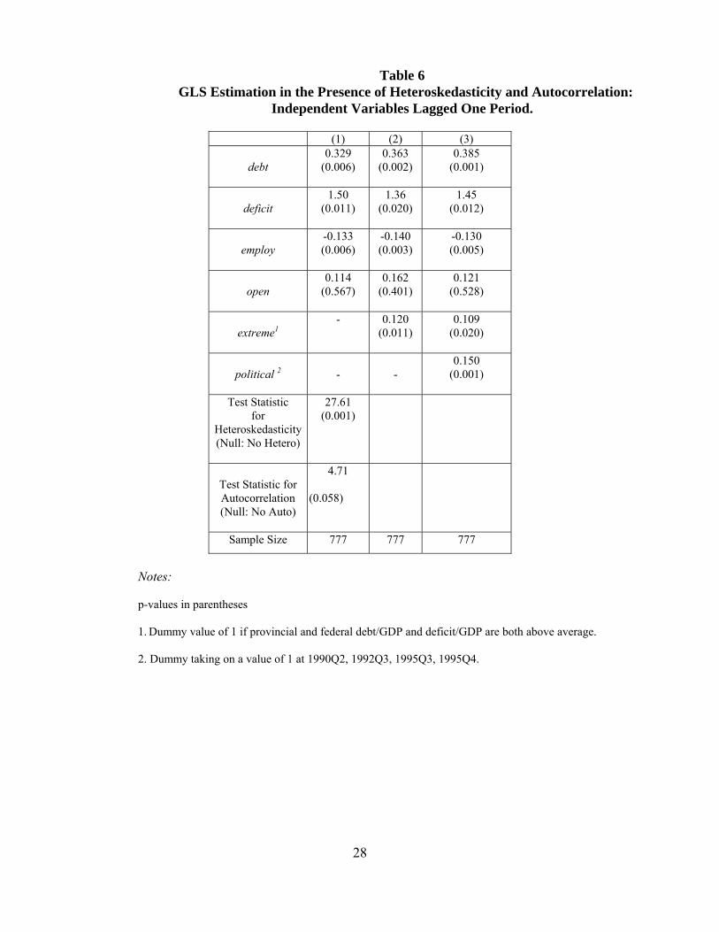
Our final check on our results is to address any potential endogeneity between the spreads and the
financial variables. To do this we use a procedure used by Ardgna et al. (2004) where we estimate
our model using one period lags of the independent variables.18 The GLS results are reported in
Table 6. The results are substantially the same, where the fiscal and political estimates are
qualitatively the same but with marginally smaller coefficients. The only difference is that the
employment variable increases in significance, while that on the openness variable declines.
Overall what is striking in the regression results is the robustness and relative stability in the
magnitude and significance of both the deficit and debt variables. Their stability is robust to
including:
• Fixed provincial effects;19 • Variables that capture wealth and revenue impacts such as employment and the
openness of the provincial economies; • Pure political uncertainty variables that capture unique events such as the collapse of
the Charlottetown and Meech Lake accords and the Quebec referendums; • GLS estimation; • Separation of Atlantic from non-Atlantic provinces; • Increased liquidity effects.
Furthermore, by including an extreme variable we confirm that the impact of financial health is
more pronounced as financial health deteriorates. This confirms the non-linearity effects of debt
and deficits alluded to in previous research. The overwhelming evidence is that the size of both
unchanged. 17. Provincial bond data is only available on an annual basis so can not be used as an independent variable. 18. Similar results are produced with variables lagged two periods. 19. Not reported but available on request.
18
provincial debt and deficits does impact provincial spreads: more debt and higher deficits cause
higher spreads consistent with the risk effects in a portfolio balance model. In contrast there is
little evidence to support a positive liquidity effect and what there is may just be proxying for other
factors.
Our final check is to examine the relationship between corporate and provincial yield spreads. As
Figure 4 shows, corporate spreads vary with the state of the business cycle and corporate
profitability. Hence, as Atkinson (1967) showed corporate spreads are indicative of general
economic conditions. However, these same cyclical effects may affect the provinces if they are
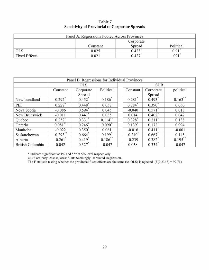
seen as possessing rescheduling risk. Table 7 shows the results of a series of regression models of
provincial yields spreads against the corporate spread and the political uncertainty dummy used
before. These estimates use monthly data as opposed to the quarterly data for the earlier results,
since the frequency of the regressors in the main empirical model were constrained by data
availability. By regressing the provincial on the corporate spread, we directly estimate the
similarity in the movement of corporate and provincial bonds.
The first model in Panel A is a simple pooled regression across provinces, and so it assumes that
investors regard all provinces as being equally sensitive to economic conditions. The slope
coefficient is 0.423 indicating that provincial bonds are less than half as sensitive as corporate
bonds to economic conditions. The slope on the political uncertainty dummy variable indicates
that uncertainty over the Quebec referendum and various constitutional crises increased provincial
spreads by an average of 91 basis points. In the second model, we allow for provincial fixed
effects. An F test on the intercepts indicates that there are distinct provincial effects.20 In Panel B,
the assumption that the sensitivity is the same across all provinces is relaxed. The first model is a
standard least squares regression for each province, while the second is a seemingly unrelated
regression (SUR) model where correlation between the contemporaneous error terms is allowed.
This essentially just recognizes that while the coefficients can differ across the provinces, each
province’s bonds are still a part of the overall bond market and likely to be buffeted by common
economic forces. The results from the OLS and SUR models are very similar to the other models.
20. For these pooled models, as well as the individual models that follow, the results without the political uncertainty dummy are almost exactly the same.
19
Overall
• The significance of the political uncertainty variable drops, and is significant for half the provinces with OLS, but only two with SUR. However, most of the coefficient estimates are positive and of similar size to previous estimates.
• The sensitivity of the provincial to corporate spreads differs significantly across provinces, indicating that investors treat these bonds differently. The least sensitive bonds are those of Ontario and Quebec. From Figure 3 these are the provinces with the most outstanding public market bonds as well as the biggest and most diverse provincial economies. However from Table 3 it is not obvious that these provinces have better financial health in terms of their deficits and debt as a share of provincial GDP.
Generally, the results indicate that investors view the smaller provinces as more sensitive to
economic conditions in spite of the fact that their financial health has not generally been
demonstrably worse than that of the larger provinces.
6. Conclusions
The analysis in this paper adds to the literature on whether or not government debt and deficits
“matter” for the yields on their public market debt. This research clearly shows that for the period
1981 to 2000 for Canadian provinces, there is strong link between provincial yield spreads and
provincial debt and deficit levels. Further we show that extreme levels of debt and deficits have an
effect over and beyond the linear effect estimated in the regression analysis. Political uncertainty
surrounding the status of Quebec also increased provincial spreads, while the openness of the
provincial economy and employment levels tend to reduce spreads. However, in the case of these
last two variables the evidence is weak and inconsistent. Finally we show that provincial debt
responds in a less exaggerated way to general economic conditions than corporate debt, implying
that provincial bonds may be weak substitutes for corporate bonds. The only possible exception to
this is the biggest issuer in the provincial bond market (and Canada’s richest province) Ontario,
where Ontario spreads are the least sensitive to corporate spreads in spite of its very large deficits
in the 1990s. This lack of sensitivity indicates that alone among Canadian provinces Ontario (and
possibly Quebec) bonds share similar qualities to government of Canada bonds, and yet even here
investors react as if they possess some rescheduling or default risk. Our results clearly indicate that
provincial yield spreads are directly related to the fiscal situation of the provinces and as a result
there are limits to the taxing powers of government.
20
Bibliography
Alesina, A., M. Broeck, A. Prati, and G. Tabellini (1992) “Default Risk on Government Debt in OECD Countries,” Economic Policy, 428-463. Amihud, Y and H. Mendelson (1991) “Liquidity, Maturity and the Yields on U.S. Government Securities,” Journal of Finance, 46, 4, 1411-1425. Atkinson, T. (1967) “Trends in Corporate Bond Quality,” National Bureau of Economic Research, NY. Ardagna, S, F. Caselli and T. Lane (2005) “Fiscal Discipline and the Cost of Public Debt service; some estimates for OECD Countries,” Working paper Harvard University, August. Barro, R. (1974) “Are Government Bonds Net Wealth?" Journal of Political Economy 82, 6, 1095-1117. Bayoumi, T, M.Goldstein, and G. Woglom (1995) “Do Credit Markets Discipline Sovereign Borrowers? Evidence from U.S. States,” Journal of Money Credit and Banking 27, 1046-1059. Bernoth, K, J. von Hagen and L. Schknecht (2004) “Sovereign risk premia in the European government bond market,” European central bank working paper #369, June. Booth, L. (1995) “Equities over Bonds, but by how much?” Canadian Investment Review, Summer 1995, 9-15, Boothe, P. (1991) "Interest Parity, Cointegration, and the Term Structure in Canada and the United States," Canadian Journal of Economics, August, 595-603. Chouinard, E. and S. Lalani (2002) “The Canadian Fixed Income Market: Recent Developments and Outlook,” Bank of Canada Review, Winter, 15-25. Dickey, D., Fuller, W. (1979) Distribution of the estimators for autoregressive time series with a unit root. Journal of the American Statistical Association 74, 427–431 Dickey, D. & W. Fuller (1981) Likelihood Ratio Statistics for Autoregressive Time Series with a Unit Root. Econometrica, 49, 1057-1072. Evans, P. (1987a) “Do Budget Deficits Raise Nominal Interest Rates? Evidence From Six Countries”, Journal of Monetary Economics 20, 281-300. Evans, P. (1987b) “Interest Rates and Expected Future Budget Deficits in the United States,” Journal of Political Economy, 95, 1, 34-58.
21
Evans, P. (1985) “Do Large Deficits Produce Higher Interest Rates?” American Economic Review 75, 1, 68-87. Fair R and B. Malkiel (1971) “The Determination of Yield Differences between Debt Instruments of the Same Maturity,’ Journal of Money Credit and Banking 3, 4, 733-749. Friedman, B. (2005) “Deficits and Debt in the short and long run,” NBER working paper September. Gauthier C, D. Tessier and V Traclet (2004) “Do Domestic macroeconomic factors play a role in determining long term interest rates? An application in the case of a small open economy” Bank of Canada working paper, May. Handa J. and B. Ma. (1989) “Four Tests for the Random Walk Hypothesis: Power versus Robustness,” Economics Letters 29, 141-145. Hejazi, W, M. Marr and J. Parkinson. (2000) “Cointegration and Canada-U.S. Term Structures: Does Accounting for Structural Breaks Make a Difference?” Canadian Journal of Administrative Sciences, vol. 17, no. 4, 342-55. Johnson, D. (1993) “International Interest Rate Linkages in the Term Structure,” Journal of Money, Credit and Banking, 25, 755-770. Johnson, D. and D. McIlraith. (1998) “Opinion polls and Canadian bond yields during the 1995 Quebec referendum campaign,” Canadian Journal of Economics vol. 31, No. 2, 411-426. Kotlikoff, L. and B. Raffelhueschen (1991) “How Regional Differences in Taxes and Public Goods Distort Life Cycle Location Choice,” NBER Working Paper 3598. Landon, S and C Smith (2000) “Government Spillovers and Creditworthiness in a Federation,” Canadian Journal of Economics, 33-3 August, 634-661. Maddala, G.S. and Wu, S., 1999. “A Comparative Study of Unit Root Tests with Panel Data and a New Simple Test “, Oxford Bulletin of Economics and Statistics, vol. 61, no. 0, Special Issue, November, pp. 631-52. Martin, P. (2001) “The Canadian Experience in Reducing Budget Deficits and Debt,” Economic Review, Federal Reserve Bank of Kansas City, Spring, 203-225. Mattina, T. and F. Delorme (1997) “The Impact of Fiscal Policy on the Risk Premium of Government Long-Term Debt: Some Canadian Evidence,” Department of Finance, Working Paper No. 97-01. Mishkin, F and A. Serletis (2005) The Economics of Money, Banking, and Financial Markets, Second Canadian Edition, Pearson Addison Wesley.
22
Mossin, J (1969) “Optimal Multiperiod Portfolio Policies,” Journal of Business, 215-229. Nunes-Correia, J and L. Stemitsiotis (1993) “Budget deficit ad interest rates: Is there a Link? International Evidence,” Commission of the European Communities Economic Papers 105, November 1993. Pedroni, Peter (1999). “Critical Values for Cointegration Tests in Heterogeneous Panels with Multiple Regressors”, Oxford Bulletin of Economics and Statistics, 61, 653-70. Phillips, P. and P. Perron (1988) “Testing for a Unit Root in a Time Series Regression,” Biometrika, 75 335-346. Plosser, C. (1987) “Fiscal Policy and the Term Structure,” Journal of Monetary Economics 20, 343-67. Plosser, C. (1982) “Government Financing Decisions and Asset Returns” Journal of Monetary Economics 9, 335-52. Scotia Capital (2004) “ Investor Guide to the Federal and Provincial Bond Markets in Canada,” May 2004. Shum, P. (1995) "The 1992 Canadian Constitutional Referendum: Using Financial Data to Access Economic Consequences", Canadian Journal of Economics, vol.28-4a, 794-807. Siklos, P. (1988) “The deficit-interest rate link: empirical evidence for Canada,” Applied Economics 20, 1563-1577. Sillamaa, M.A. and E. Olson. (2003) “Marginal Tax Rates and Interprovincial Migration”, Statistics Canada Working Paper. Van Horne, J.C. (1978) Financial Market Rates and Flows, Englewood Cliffs, NJ, Prentice Hall. Wooldridge, J. (2002) “Econometric Analysis of Cross Section and Panel Data”. MIT Press
Source: Chouinard et al. (2002) updated for 2002 and 2003.
Provincials include Municipal bonds. Turnover is defined as the annual average based on weekly trading volume divided by the outstanding stock of bonds.
24
Table 2 Descriptive Statistics: Provincial and Canada Yields and Provincial-Canada Spreads
Table 4. GLS Estimation in the Presence of Heteroskedasticity and Autocorrelation;
Determinants of the Provincial Spread
Panel A Panel B Panel C (1) (2) (3) (1) (2) (3) (1) (2) (3)
debt 0.543
(0.001)
0.566 (0.001)
0.566 (0.001)
0.654 (0.001)
0.687 (0.001)
0.690 (0.001)
0.411 (0.001)
0.418 (0.001)
0.422 (0.001)
deficit 2.69
(0.001)
2.50 (0.001)
2.59 (0.001)
2.80 (0.001)
2.64 (0.001)
2.73 (0.001)
3.04 (0.001)
2.87 (0.001)
2.94 (0.001)
employ
-0.037 (0.429)
-0.046 (0.305)
-0.044(0.324)
-0.090 (0.130)
-0.105 (0.061)
-0.103 (0.061)
0.115 (0.158)
0.117 (0.124)
0.117 (0.120)
open
-0.484 (0.015)
-0.416 (0.030)
-0.429(0.023)
-0.524 (0.009)
-0.467 (0.016)
-0.482 (0.011)
-0.641 (0.003)
-0.570 (0.005)
-0.580 (0.004)
extreme1
- 0.104 (0.028)
0.093 (0.046)
-
0.109 (0.020)
0.098 (0.033)
- 0.113 (0.014)
0.102 (0.026)
political 2
-
-
0.152 (0.001)
-
-
0.153 (0.001)
-
-
0.152 (0.001)
Equal. Payments Dummy
- - - -0.120 (0.171)
-.137
(0.101)
-0.139 (0.089)
- - -
Atlantic Dummy 0.238 (0.015)
0.264 (0.004)
0.260 (0.004)
Sample Size 786 786 786 786 786 786
786 786 786 Notes:
p-values in parentheses There is no R-squared statistic reported because such a statistic is not meaningful in GLS. See footnote 15. 1. This dummy variable takes on a value of 1 if provincial and federal debt/GDP and deficit/GDP are both above average, and zero otherwise. 2. This dummy variable takes on a value of 1 for the periods 1990Q2, 1992Q3, 1995Q3, 1995Q4, and zero otherwise.
27
Table 5
Fixed Effects Intercepts and Outstanding Debt
FE Constant
(relative to BC)
1981 Bonds $Cmm
1990 Bonds $Cmm
2002 Bonds $Cmm
1981 Ratio to
BC
1990 Ratio to
BC
2002 Ratio to
BC
Newfoundland
-2.25 2252 4581 6402 1.06 0.66 0.20
PEI
-3.79 257 618 1110 0.12 0.09 0.03
Nova Scotia
-1.64 2156 6526 13216 1.01 0.95 0.41
New Brunswick -2.17 1597 4677 11493 0.75 0.68 0.35 Quebec
0.84 9194 25408 64474 4.32 3.68 1.98
Ontario
1.32 20723 45180 92631 9.73 6.54 2.85
Manitoba
-1.50 2652 9224 15288 1.25 1.34 0.47
Saskatchewan
-1.54 2480 8606 10448 1.16 1.25 0.32
Alberta
-0.38 5030 12988 8182 2.36 1.88 0.25
BC
n/a 2129 6903 32520
Correlation between the fixed effects constant and the ratio of provincial debt to that of BC varies from 0.86 to 0.90. All fixed effects constant have p values of < 0.001.
28
Table 6 GLS Estimation in the Presence of Heteroskedasticity and Autocorrelation:
Independent Variables Lagged One Period.
(1) (2) (3)
debt 0.329
(0.006)
0.363 (0.002)
0.385 (0.001)
deficit
1.50 (0.011)
1.36 (0.020)
1.45 (0.012)
employ
-0.133 (0.006)
-0.140 (0.003)
-0.130 (0.005)
open
0.114 (0.567)
0.162 (0.401)
0.121 (0.528)
extreme1
- 0.120 (0.011)
0.109 (0.020)
political 2
-
-
0.150 (0.001)
Test Statistic for
Heteroskedasticity (Null: No Hetero)
27.61 (0.001)
Test Statistic for Autocorrelation (Null: No Auto)
4.71 (0.058)
Sample Size 777 777 777
Notes: p-values in parentheses
1. Dummy value of 1 if provincial and federal debt/GDP and deficit/GDP are both above average.
2. Dummy taking on a value of 1 at 1990Q2, 1992Q3, 1995Q3, 1995Q4.
29
Table 7 Sensitivity of Provincial to Corporate Spreads
0.038 0.334* -0.047 * indicate significant at 1% and *** at 5% level respectively. OLS: ordinary least squares; SUR: Seemingly Unrelated Regression.
The F statistic testing whether the provincial fixed effects are the same (ie. OLS) is rejected (F(9,2347) = 99.71).
30
Figure 1
Panel A. All 2003 Outstanding Debt Issues in C$ mm (Total size of the bond market: $1,202 billion)
Canadian Issuer Bond Market
Canadas, $315,385, 26%
Provinces, $354,710, 30%
Municipal, $31,201, 3%
Corp, $404,852, 33%
Securitised, $93,095, 8%
Other, $2,935, 0%
Panel B. Trends in Provincial Share of the Bond Market (based on all issues)
20.00
25.00
30.00
35.00
40.00
45.00
1977
1979
1981
1983
1985
1987
1989
1991
1993
1995
1997
1999
2001
2003
%
Bank of Canada Banking and Financial Statistics Tables G6 and K8) (Bank of Canada Banking and Financial Statistics Tables G6 and K8 for various years)
31
Figure 2
Government Surpluses Statistics Canada Cansim series D14816, D2000, D 15075, D 20171
-10.00
-8.00
-6.00
-4.00
-2.00
0.00
2.00
4.00
6.00
"195
0"
"195
3"
"195
6"
"195
9"
"196
2"
"196
5"
"196
8"
"197
1"
"197
4"
"197
7"
"198
0"
"198
3"
"198
6"
"198
9"
"199
2"
"199
5"
"199
8"
"200
1
% o
f GD
P
32
Figure 3
2003 Provincial Bond Market Total size $354.7 billion.
New2%
Ontario37%
NS4%NB
3%0%
Quebec32%
Manitoba5%
Saskatchewan3%
Alberta3%
BC11%
Bank of Canada Banking and Financial Statistics Table K8 For presentation purposes we have used the following abbreviations: BC is British Columbia New is Newfoundland, NB is New Brunswick, NS is Nova Scotia, Unmarked (less than 1.0%) is Prince Edward Island, the Yukon and the Territories.
33
Figure 4
Corporate Spreads and Profitability Cansim D86221 and Scotia Capital Markets, Handbook of Canadian Debt Market Indicators, Feb 2004.
The right axis is the ROE and the left the BBB spread over equivalent maturity Canada bonds.
Corporate ROE and BBB Spread
050
100150200250300350400
1980
1982
1984
1986
1988
1990
1992
1994
1996
1998
2000
2002
basi
s po
ints
0.002.004.006.008.0010.0012.0014.0016.00
Per
cent
BBB Spread ROE
34
Figure 5
History of Provincial and Corporate Spreads over Equivalent Maturity Canada bonds
Cansim data labels V121759, V121761 V121791 (A similar graph appears in Mishkin and Serletis (2005))