This paper presents preliminary findings and is being distributed to economists and other interested readers solely to stimulate discussion and elicit comments. The views expressed in this paper are those of the authors and do not necessarily reflect the position of the Federal Reserve Bank of New York or the Federal Reserve System. Any errors or omissions are the responsibility of the authors. Federal Reserve Bank of New York Staff Reports When Does a Central Bank’s Balance Sheet Require Fiscal Support? Marco Del Negro Christopher A. Sims Staff Report No. 701 November 2014 Revised March 2015
Transcript
This paper presents preliminary findings and is being distributed to economists
and other interested readers solely to stimulate discussion and elicit comments.
The views expressed in this paper are those of the authors and do not necessarily
reflect the position of the Federal Reserve Bank of New York or the Federal
Reserve System. Any errors or omissions are the responsibility of the authors.
Federal Reserve Bank of New York
Staff Reports
When Does a Central Bank’s Balance Sheet
Require Fiscal Support?
Marco Del Negro
Christopher A. Sims
Staff Report No. 701
November 2014
Revised March 2015
When Does a Central Bank’s Balance Sheet Require Fiscal Support? Marco Del Negro and Christopher A. Sims
Federal Reserve Bank of New York Staff Reports, no. 701
November 2014; revised March 2015
JEL classification: E58, E59
Abstract
Using a simple general equilibrium model, we argue that it would be appropriate for a central
bank with a large balance sheet composed of long-duration nominal assets to have access to, and
be willing to ask for, support for its balance sheet by the fiscal authority. Otherwise, its ability to
control inflation may be at risk. This need for balance sheet support—a within-government
transaction—is distinct from the need for fiscal backing of inflation policy that arises even in
models where the central bank’s balance sheet is merged with that of the rest of the government.
Key words: central bank’s balance sheet, solvency, monetary policy
_________________
Del Negro: Federal Reserve Bank of New York (e-mail: [email protected]). Sims:
Princeton University (e-mail: [email protected]). This paper was presented at the November
2014 Carnegie-Rochester-NYU Conference on Public Policy. The authors are grateful to their
discussant, Ricardo Reis, and to Marvin Goodfriend, the special editor, for their thoughtful
suggestions. The authors also thank Fernando Alvarez, Marco Bassetto, Seth Carpenter, Behzad
Diba, William Roberds, Andreas Schabert, Oreste Tristani, Harald Uhlig, and participants at
various seminars and conferences for very helpful comments. The views expressed in this paper
are those of the authors and do not necessarily reflect the position of the Federal Reserve Bank of
New York or the Federal Reserve System.
CENTRAL BANK’S BALANCE SHEET 1
I. INTRODUCTION
Hall and Reis (2013) and Carpenter, Ihrig, Klee, Quinn, and Boote (2013)
have explored the likely path of the Federal Reserve System’s balance sheet
during a possible return to historically normal levels of interest rates. Both
conclude that, though a period when the system’s net worth at market value
is negative might occur, this is unlikely, would be temporary and would not
create serious problems.1 Those conclusions rely on extrapolating into the
future not only a notion of historically normal interest rates, but also of
historically normal relationships between interest rates, inflation rates, and
components of the System’s balance sheet.
In this paper we look at complete, though simplified, economic mod-
els in order to study why a central bank’s balance sheet matters at all and
the consequences of a lack of fiscal support for the central bank. Unlike
some of the previous literature, we are not just concerned about periods of
zero remittances to the fiscal authority. Rather, we ask whether the lack of
fiscal support (that is, a commitment by the fiscal authority never to recap-
italize the central bank) implies that the central bank is no longer able to
maintain control of inflation, because doing so would lead to its insolvency.
These issues are important because they lead us to think about unlikely, but
nonetheless possible, sequences of events that could undermine economic
stability. As recent events should have taught us, historically abnormal
1Christensen, Lopez, and Rudebusch (2013) study the interest rate risk faced by the Fed-
eral Reserve using probabilities for alternative interest rate scenarios obtained from a dy-
namic term structure model. They reach the similar conclusions as Hall and Reis (2013) and
Carpenter, Ihrig, Klee, Quinn, and Boote (2013). Greenlaw, Hamilton, Hooper, and Mishkin
(2013) conduct a similar exercise as Carpenter, Ihrig, Klee, Quinn, and Boote (2013), but also
consider scenarios where concern about the solvency of the U.S. government lead to capital
losses for the central bank.
CENTRAL BANK’S BALANCE SHEET 2
events do occur in financial markets, and understanding in advance how
they can arise and how to avert or mitigate them is worthwhile.2
Constructing a model that allows us to address these issues requires us
to specify monetary and fiscal policy behavior and to consider how demand
for non-interest-bearing liabilities of the central bank (like currency, or re-
quired reserves paying zero interest) responds to interest rates. As we show
below, seigniorage plays a central role in determining the possible need for
fiscal support for the central bank. But with a given policy in place, seignior-
age can vary widely, depending on how sharply demand for cash shrinks
as inflation and interest rates rise. An equilibrium model with endogenous
demand for cash is therefore required if we are to understand the sources
and magnitudes of possible central bank balance sheet problems.
In the first section below we consider a stripped down model to show
how the need for fiscal support arises. In subsequent sections we make the
model more realistic and try to determine how likely it is that the US Federal
Reserve System will need fiscal support. In both the simple model and the
more realistic one, we make some of the same generic points.
For the price level to be uniquely determined, fiscal policy must be seen
to “back” the price level. Our first point consists in distinguishing this
“backing” from what we call fiscal “support”. The central bank cannot on its
2Work by Peter Stella (2005b; 2005a) was among the earliest to bring out the potential im-
portance of central bank balance sheets . A number of recent papers, including Buiter and
Rahbari (2012), Corsetti and Dedola (2012), Bassetto and Messer (2013a), Benigno and Nis-
ticó (2014), and Reis (2013), also study the central bank’s and the fiscal authorities’ balance
sheets separately. Bhattarai, Eggertsson, and Gafarov (2013) discuss how the acquisition
of long-term government debt by the central banks affects its incentives in terms of set-
ting interest rates. Finally, Quinn and Roberds (2014) provide an interesting account of
the demise of the Florin as an international reserve currency in the late 1700s and attribute
such demise to the central bank’s credit policies and a belated and inadequate recognition
that it needed fiscal backing.
CENTRAL BANK’S BALANCE SHEET 3
own provide fiscal backing. Cochrane (2011) has made this point carefully.
Fiscal backing requires that explosive inflationary or deflationary behavior
of the price level is seen as impossible because the fiscal authority will re-
spond to very high inflation with higher primary surpluses and to near-zero
interest rates with lower, or negative, primary surpluses. But even when fis-
cal policy is in place that guarantees the price level is uniquely determined
and the behavior of inflation is driven by monetary policy, it is nonetheless
possible that the central bank, if its balance sheet is sufficiently impaired,
may need recapitalization in order to maintain its commitment to a policy
rule or an inflation target. Such a recapitalization is a within-government
transaction, unrelated to whether fiscal backing is present. Fiscal “support”
is what we call a commitment by the treasury to recapitalize the central bank
if necessary. Without fiscal support, a central bank that could otherwise im-
plement its policy rule or hit its inflation target, may find that it must allow
more inflation than it would like.
Second, a central bank’s ability to earn seigniorage can make it possi-
ble for it to recover from a situation of negative net worth at market value
without recapitalization from the treasury, while still maintaining its policy
rule. Whether it can do so depends on the policy rule, the demand for its
non-interest-bearing liabilities, and the size of the initial net worth gap.3
Last, in the presence of a large long-duration balance sheet, a central
bank that is committed to avoiding any request for fiscal support (or a fiscal
authority committed to providing none) can open the door to indetermi-
nacy via self-fulfilling equilibria. Expectations of high inflation in the future
can lead to capital losses that need to be filled by generating seigniorage,
thereby validating the expectations.3Berriel and Bhattarai (2009) study optimal policy in a setting where the central bank
and the fiscal authority have separate budget constraints. Berriel and Bhattarai (2009) only
consider the case where the central bank can acquire short-term assets however, which
implies that solvency issues are unlikely to arise (see Bassetto and Messer (2013b)).
CENTRAL BANK’S BALANCE SHEET 4
II. THE SIMPLE MODEL
We first consider a stripped-down model to illustrate the principles at
work. A representative agent solves
maxC,B,M,F
∫ ∞
0e−βt log(Ct) dt subject to (1)
Ct · (1 + ψ(vt)) +B + M
Pt+ τt + Ft = ρFt +
rtBt
Pt+ Yt , (2)
where C is consumption, B is instantaneous nominal bonds paying interest
at the rate r, M is non-interest-bearing money, ρ is a real rate of return on
a real asset F, Y is endowment income, and τ is the primary surplus (or
simply lump-sum taxes, since we have no explicit government spending in
this model). Velocity vt is given by
vt =PtCt
Mt, vt ≥ 0, (3)
and the function ψ(.), ψ′(.) > 0 captures transaction costs.
The government budget constraint is
B + MPt
+ τt =rtBt
Pt. (4)
Monetary policy is an interest-smoothing Taylor rule:
r = θr ·(
r + θπ
( PP− π
)− r)
. (5)
The “Taylor Principle”, that θπ should exceed one, is the usual prescription
for “active” monetary policy. The effective short term interest rate is given
by the maximum of rt and the lower bound on interest rates r:
ret = max (rt, r) . (6)
CENTRAL BANK’S BALANCE SHEET 5
First order conditions for the private agent are
∂C :1C
= λ(1 + ψ + ψ′v) (7)
∂F : − ˆλ = λ(ρ− β) (8)
∂B : −ˆλP+ β
λ
P+
λ
P
ˆPP= r
λ
P(9)
∂M : −ˆλP+ β
λ
P+
λ
P
ˆPP=
λ
Pψ′v2 (10)
The ˆzt notation means the time derivative of the future expected path of z
at t. It exists even at dates when z has taken a jump, so long as its future
path is right-differentiable. Below we also use the d+dt operator for the same
concept.
We are taking the real rate ρ as exogenous, and in this simple version of
the model constant. The economy is therefore being modeled as either hav-
ing a constant-returns-to scale investment technology or as having access to
international borrowing and lending at a fixed rate. Though we could ex-
tend the model to consider stochastically evolving Y, ρ, and other external
disturbances, here we consider only surprise shifts at the t = 0 starting date,
with perfect-foresight deterministic paths thereafter. This makes it easier
to follow the logic, though it makes the time-0 adjustments unrealistically
abrupt.
Besides the exogenous influences that already appear explicitly in the
system above (ρ and Y), we consider an “inflation scare”4 variable x. This
enters the agents’ first order condition as a perturbation to inflation expec-
tations. It can be reconciled with rational expectations by supposing that
agents think there is a possibility of discontinuous jumps in the price level,
with these jumps arriving as a Poisson process with a fixed rate. This would
happen if at these jump dates monetary policy created discontinuous jumps
4Goodfriend (1993) coined the term “inflation scare” for a phenomenon like what we
model here and pointed to historical episodes where they seem to have occurred.
CENTRAL BANK’S BALANCE SHEET 6
in M. Such jumps would create temporary declines in the real value of gov-
ernment debt B/P and would generate seigniorage, which might explain
why such jumps are perceived as possible. If the jump process doesn’t
change after a jump occurs, there is no variation in velocity, the inflation
rate, consumption, or the interest rate at the jump dates. We consider two
versions of an inflation scare: One in which the public is correct about the
occurrence of occasional randomly timed price level jumps (so seigniorage
is higher) and one in which they are incorrect, with central bank policy stick-
ing to the Taylor rule at all times. In the latter case, of course, private agents
would eventually be likely to revise their expectations, and we do not for-
mally model that. But since the public’s beliefs are consistent with no price
jumps over any finite span of time, there is no logical problem with assum-
ing that they hold to those beliefs over a long period of time with no price
jumps.
The inflation scare variable changes the first order conditions above to
give us
∂B : − ˆλ1P+ β
λ
P+
λ
P
(ˆPP+ x
)= r
λ
P(9’)
∂M : − ˆλ1P+ β
λ
P+
λ
P
(ˆPP+ x
)=
λ
Pψ′v2 (10’)
Because the price and money jumps have no effect on interest rates or con-
sumption, no other equations in the model need change. These first or-
der conditions reflect the private agents’ use of a probability model that
includes jumps in evaluating their objective function.
We can solve the model analytically to see the impact of an unantici-
pated, permanent, time-0 shift in ρ (the real rate of return), x (the inflation
scare variable), or r (the central bank’s interest-rate target). We could also
CENTRAL BANK’S BALANCE SHEET 7
solve it numerically for arbitrary time paths of ρ, x, r, et cetera, but we re-
serve such exercises for the more detailed and realistic model in subsequent
sections.
Solving to eliminate the Lagrange multipliers from the first order condi-
tions we obtain
ρ = r−ˆPP− x (11)
r = ψ′(v)v2 (12)
− d+
dt
(1
C · (1 + ψ + ψ′v)
)=
ρ− β
C(1 + ψ + ψ′v). (13)
Using (11) and the policy rule (5), we obtain that along the path after the
initial date,
r = θr · ((θπ(r− ρ− x)− r + r− θππ)
= θr · (θπ − 1)r− θrθπ(ρ + x) + θr(r− θππ) . (14)
With the usual assumption of active monetary policy, θπ > 1, so this is an
unstable differential equation in the single endogenous variable r. Solutions
are of the form
rt = Et
[∫ ∞
0e−(θπ−1)θrsθrθπ(ρt+s + xt+s) ds
]− r− θππ
θπ − 1+ κe(θπ−1)θrt. (15)
In a steady state with x and ρ constant (and κ = 0), this give us
r =θπ(ρ + x)
θπ − 1− r− θππ
θπ − 1. (16)
From (12) we can find v as a function of r. Substituting the government bud-
get constraint into the private budget constraint gives us the social resource
constraint
C · (1 + ψ(v)) + F = ρF + Y. (17)
Solving this unstable differential equation forward gives us
Ft = Et
[∫ ∞
0exp
(−∫ s
0ρt+v dv
)(Yt+s − Ct+s(1 + ψ(vt+s))) ds
]. (18)
CENTRAL BANK’S BALANCE SHEET 8
Here we do not include an exponentially explosive term because that would
be ruled out by transversality in the agent’s problem and by a lower bound
on F. With constant ρ, x and Y, r and v are constant, and (13) then lets
us conclude that C grows (or shrinks) steadily at the rate ρ − β. We can
therefore use (18) to conclude that along the solution path, since ρ, Y and v
are constant
Ct =β · (ρ−1Y + Ft)
1 + ψ(v). (19)
This lets us determine initial C0 from the F0 at that date. From then on Ct
grows or shrinks at the rate ρ − β and the resulting saving or dissaving
determines the path of Ft from (19).
Whether in steady state or not, knowing the time path of r (as a function
of κ) from (15) gives us the time path for v from (12), for C from (18) and
(13) and then real balances m from the definition of v. We then get inflation
from (11). But a time path for inflation does not give us a value for P0, the
initial price level. The indeterminacy in P is only through its dependence
on κ, however. We interpret the Taylor rule (5) as not forward-looking —
that is, it holds locally, with left and right derivatives equal, at all dates,
including the initial date. But this assumed differentiability applies to the
linear combination of derivatives that appear in the equation: r− θrθπ P/P.
Thus while the equation implies r− log P is differentiable from left and right
even at time zero, it does not constrain r and P individually from jumping.
Our solution for r as given in (15) is forward-looking and generally implies
an initial discontinuous jump in r at time 0. The Taylor rule then determines
a corresponding initial jump in the price level, determining P0 — except
that, because κ enters (15), P0 depends on κ. Note that whenever κ 6= 0, r
eventually explodes at an exponential rate, implying via (11) that inflation
(not the price level) explodes exponentially.
CENTRAL BANK’S BALANCE SHEET 9
III. FISCAL BACKING AND FISCAL SUPPORT
The literature on the fiscal theory of the price level has shown that mon-
etary policy alone cannot uniquely determine the price level without appro-
priate fiscal backing (Cochrane, 2011) . This literature, though, for the most
part distinguishes monetary policy and fiscal policy only by what variables
they control — interest rates or money growth for the former, taxes and
spending for the latter. The government is treated as having a unified bud-
get constraint, with no separate accounting of assets and liabilities of the
central bank vs. those of the fiscal authority.
The model of the previous section, which we will identify as the “sim-
ple model”, also has only a unified government budget constraint. Further-
more, we have so far specified only a government budget constraint, not a
fiscal policy rule. In this model, and in the more complex model discussed
below, the insights of the fiscal theory of the price level apply. A Taylor
rule monetary policy, even if it satisfies the θπ > 1 condition, cannot by it-
self uniquely determine the price level. This is reflected in the fact that we
cannot rule out κ 6= 0 in (15) in equilibrium.
Though this point about non-uniqueness of the price level is by now
well known (if not completely non-controversial), the fiscal “support” we
are discussing in this paper is not the fiscal “backing” whose necessity is
brought out in the fiscal theory of the price level. To pin down a unique
price level requires a fiscal policy – in this model a rule for setting the pri-
mary surplus — that provides the backing. Under some conditions, fiscal
backing can take a form that forces κ to zero, and hence leaves the time
path of prices to be determined by monetary policy, without reference to
the details of the fiscal policy rule.
Most of the analysis in this paper assumes that fiscal backing is present
and determines κ uniquely, in most but not all cases determines it uniquely
CENTRAL BANK’S BALANCE SHEET 10
as zero. Yet we still discuss the need for fiscal “support”, because we con-
sider a central bank balance sheet and budget in addition to those of the
unified government. Fiscal support is needed when the central bank cannot
maintain its desired inflation policy or its policy rule without a capital injec-
tion from the treasury. Since such a capital injection would most naturally
take the form of transferring nominal, interest-bearing government bonds
from the treasury to the central bank, the unified government budget and
balance sheet would net out the transaction. And indeed, if the transaction
took place automatically and smoothly, it would be of no concern to policy.
But in some countries and time periods, including perhaps the US now, the
need for a fiscal transfer for recapitalization could have important political
economy consequences, particularly for central bank independence.
We defer to the appendix detailed discussion of the fiscal policies that
can deliver a unique value of κ in our model, but discuss the issue infor-
mally here. As we have already verified, the simple model without specify-
ing a fiscal policy rule delivers the conclusion that the price level either fol-
lows a path with stable inflation, or, with κ 6= 0 follows a path with inflation
exploding. Economists often rule out highly explosive solutions to dynamic
models by an appeal to “transversality” and “no-Ponzi” conditions. Why
does that not work here?
Transversality conditions are implications of dynamic optimization. They
rule out model solutions in which wealth grows without bound, while ex-
penditures that deliver utility remain bounded or grow much more slowly.
In the simple model, the transversality condition of the private agent re-
quires that private wealth in the form of real government debt B/P not
grow, relative to C · (1 + ψ + ψ′v), at faster than the discount rate β. But
the model solutions in which κ 6= 0 imply only that nominal interest rates
and inflation explode. With some forms of fiscal policy, the real value of
government debt remains stable despite the explosion in nominal rates and
CENTRAL BANK’S BALANCE SHEET 11
inflation. Transversality, which rules out rapidly growing wealth, and no-
Ponzi conditions, which rule out paths on which the public starts borrowing
from the government instead of investing in its debt, are then satisfied even
on the explosive paths.
In order to deliver a unique value of κ when monetary policy follows
a Taylor rule with θπ > 1, fiscal policy, which conventionally is specified
as not depending on inflation, must be seen as responsive to inflation, at
least at very high and very low rates of inflation. Fiscal policy must tighten
in response to increased inflation at high inflation rates, and loosen (run
deficits) at low inflation rates, as deflation approaches −ρ. If it is seen as
committed to respond this way, it can eliminate all the κ 6= 0 equilibria,
thereby ensuring stable inflation, and thus never requiring that inflation
reach levels that impact fiscal policy in equilibrium.5
IV. HOW COULD A CENTRAL BANK BE “INSOLVENT”?
A central bank in an economy with fiat money by definition can always
pay its bills by printing money. In that sense it cannot be insolvent. On the
other hand, paying its bills by printing money clearly could interfere with
the policy objectives of the central bank, assuming it wants to control in-
flation. Historically there were central banks (like the US Federal Reserve
in previous decades) whose liabilities were all reasonably characterized as
“money”. There was currency, which paid no interest, and also reserve de-
posits, which also paid no interest. For such a central bank it is easy to
5Cochrane (2011) might seem to contradict this paragraph’s assertion, as he apparently
suggests that there is no way for a Taylor rule to deliver a determinate price level. He
agrees, though, that there are fiscal policies that will deliver a determinate price level.
Where he might disagree is on whether policies like those we propose in the appendix,
which commit to actions at high and low inflation levels that are not observed in equilib-
rium, can be credibly implemented.
CENTRAL BANK’S BALANCE SHEET 12
understand that “paying bills by printing money” could conflict with “re-
stricting money growth to control inflation”.
Modern central banks, though, have interest-bearing reserve deposit lia-
bilities as well as non-interest-bearing ones. Furthermore, in the last several
years central banks have demonstrated that they can rapidly expand their
reserve deposit liabilities without generating strong inflationary pressure.
Such central banks can “print” interest-bearing reserves. What prevents
them from meeting any payment obligations they face by creating interest-
bearing reserve deposits?
The recent non-inflationary balance sheet expansions have arisen through
central bank purchases of interest-earning assets by issuing interest-bearing
reserves. If instead it met payment obligations — staff salaries, plant and
equipment, or interest on reserves — by issuing new interest-bearing re-
serve deposits, there would be no flow of earnings from assets offsetting
the new flow of interest on reserves. If this went on long enough, interest-
bearing liabilities would come to exceed interest-bearing assets. To the ex-
tent the gap between interest earnings and interest-bearing obligations was
not covered by seignorage, the bank’s net liabilities would begin growing
at approximately the interest rate.
In this scenario, the private sector would be holding an asset — reserves
— that was growing at the real interest rate. This might be sustainable if
there were some offsetting private sector liability growing at the same rate
— expected future taxes, or bonds issued by the private sector and bought
by the government, for example. But if we rule out these possibilities, by
saying real taxes are bounded and the fiscal authority will not accumulate
an exponentially growing cache of private sector debt, the exploding liabil-
ities of the central bank violate the private sector’s transversality condition.
In other words, private individuals, finding their assets growing so rapidly,
would try to turn those assets into consumption goods. Or in still other
CENTRAL BANK’S BALANCE SHEET 13
words, the exploding interest-bearing liabilities of the central bank would
eventually cause inflation, even if money supply growth were kept low.
This conclusion is a special case of the usual analysis in the fiscal theory
of the price level: increased issue of nominal bonds, unbacked by taxation,
is eventually inflationary, regardless of monetary policy.
V. CAPITAL LOSSES FROM INTEREST RATE INCREASES IN THE SIMPLE
MODEL
In this section we show how the central bank balance sheet and capital
needs respond to one-time, unanticipated increases in the interest rate, with
two different assumptions on the source of the interest rate change. In one
the real rate changes, while in the other the nominal rate changes because
of an inflation scare, with no change in the real rate.
We are interested in determining the effects of these one-time distur-
bances in exogenous elements of the model on the central bank balance
sheet and on the sustainability of its policy rule. We need therefore to
specify the central bank’s balance sheet. We assume that it holds as assets
nominal government debt, in the nominal amount BC. It has non-interest-
bearing liabilities M (currency) and interest-bearing liabilities (reserves) V.
The assets have duration ω > 0. We assume that along the perfect-foresight
equilibrium path V and BC pay the same rate of return, but since V are as-
sumed to be demand liabilities (deposits) with duration 0, their value is not
affected by changes in interest rates. We hold for later, in the discussion
of the larger model, precise specification of the maturity structure of the
debt. For our comparative steady state calculation what matters is only that
when, unexpectedly, the interest rate changes from one constant level r to a
new constant level r′, the price q of assets of duration ω changes by a factor
(ωr + 1)/(ωr′ + 1). A need for recapitalization arises when qBC − V be-
comes negative, while the discounted present value of seigniorage remains
CENTRAL BANK’S BALANCE SHEET 14
too small to cover the gap. For comparison of steady states in this sim-
ple model, the discounted present value of seigniorage is M0π/r, where all
variables are at their time-zero values after any initial discontinuous jumps.
To make the calculations, we need to specify the form of ψ(v), the trans-
actions cost function. We choose the form
ψ(v) = ψ0e−ψ1/v . (20)
Our reasons for choosing this functional form, and the extent of its claim
to realism, are discussed below in the context of the detailed model. We
use ψ0 = 50, ψ1 = 103. The ψ1 value matches the base case of the detailed
model, while the ψ0 value is adjusted to reflect the fact that here we nor-
malize Y and M to 1. We set the policy parameters θπ = 1.5, θr = 1, r = ρ,
π = .005. It is also assumed that Y = 1, F0 = 0, and initial M = 1.
First we look at a change from ρ = β = r = .01 to ρ = β = .02. This
is meant to crudely approximate an interest rate increase arising out of a
cyclical recovery. We increase β and ρ together because in our setup, with a
fixed real rate, changing the gap between ρ and β has large effects on initial
savings and consumption that would not be nearly as strong if we had a
model with endogenous real rate.
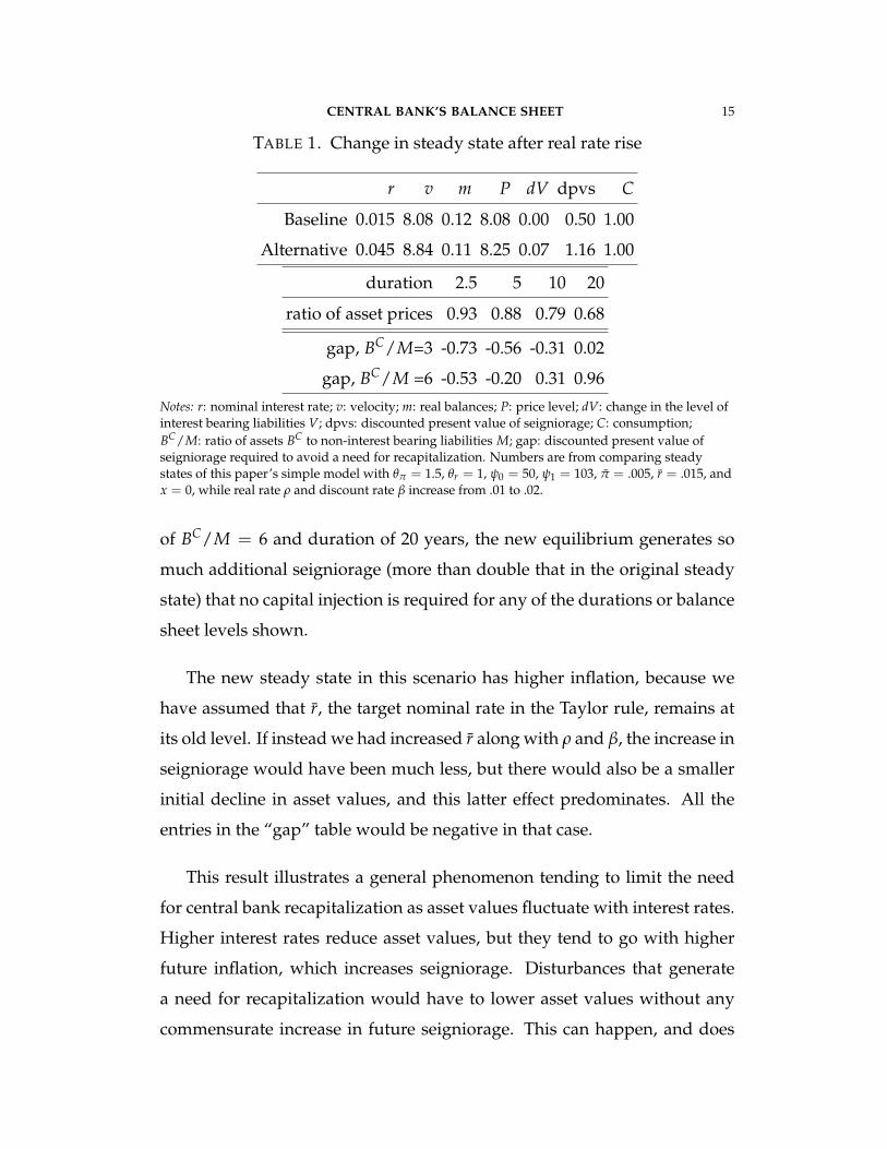
Table 1 shows that such a rise in real rate can have a big impact on
the balance sheet, yet nonetheless require no capital injection. Asset val-
ues decline by 7% to 32%, depending on duration. Interest-bearing liabil-
ities rise and nominal balances fall as private agents reduce money hold-
ings in response to the higher interest rates. This is enough to push the
central bank’s assets below V, meaning that net interest earnings will be
negative in the new steady state, but only when BC/M is six times M and
with durations longer than 5 years or, marginally, when duration is 20 and
asets are 3 times M. Yet, despite the large interest earnings gap, amount-
ing in present value to nearly the value of outstanding currency in the case
CENTRAL BANK’S BALANCE SHEET 15
TABLE 1. Change in steady state after real rate rise
r v m P dV dpvs C
Baseline 0.015 8.08 0.12 8.08 0.00 0.50 1.00
Alternative 0.045 8.84 0.11 8.25 0.07 1.16 1.00
duration 2.5 5 10 20
ratio of asset prices 0.93 0.88 0.79 0.68
gap, BC/M=3 -0.73 -0.56 -0.31 0.02
gap, BC/M =6 -0.53 -0.20 0.31 0.96
Notes: r: nominal interest rate; v: velocity; m: real balances; P: price level; dV: change in the level ofinterest bearing liabilities V; dpvs: discounted present value of seigniorage; C: consumption;BC/M: ratio of assets BC to non-interest bearing liabilities M; gap: discounted present value ofseigniorage required to avoid a need for recapitalization. Numbers are from comparing steadystates of this paper’s simple model with θπ = 1.5, θr = 1, ψ0 = 50, ψ1 = 103, π = .005, r = .015, andx = 0, while real rate ρ and discount rate β increase from .01 to .02.
of BC/M = 6 and duration of 20 years, the new equilibrium generates so
much additional seigniorage (more than double that in the original steady
state) that no capital injection is required for any of the durations or balance
sheet levels shown.
The new steady state in this scenario has higher inflation, because we
have assumed that r, the target nominal rate in the Taylor rule, remains at
its old level. If instead we had increased r along with ρ and β, the increase in
seigniorage would have been much less, but there would also be a smaller
initial decline in asset values, and this latter effect predominates. All the
entries in the “gap” table would be negative in that case.
This result illustrates a general phenomenon tending to limit the need
for central bank recapitalization as asset values fluctuate with interest rates.
Higher interest rates reduce asset values, but they tend to go with higher
future inflation, which increases seigniorage. Disturbances that generate
a need for recapitalization would have to lower asset values without any
commensurate increase in future seigniorage. This can happen, and does
CENTRAL BANK’S BALANCE SHEET 16
happen, when bad judgment or political pressure leads a central bank to
invest in assets of insolvent private entities, but our formal model does not
take up this possibility.
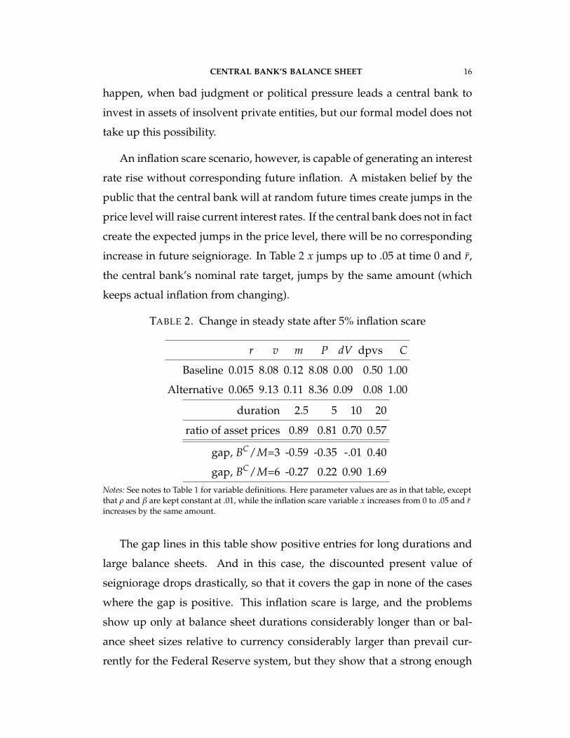
An inflation scare scenario, however, is capable of generating an interest
rate rise without corresponding future inflation. A mistaken belief by the
public that the central bank will at random future times create jumps in the
price level will raise current interest rates. If the central bank does not in fact
create the expected jumps in the price level, there will be no corresponding
increase in future seigniorage. In Table 2 x jumps up to .05 at time 0 and r,
the central bank’s nominal rate target, jumps by the same amount (which
keeps actual inflation from changing).
TABLE 2. Change in steady state after 5% inflation scare
r v m P dV dpvs C
Baseline 0.015 8.08 0.12 8.08 0.00 0.50 1.00
Alternative 0.065 9.13 0.11 8.36 0.09 0.08 1.00
duration 2.5 5 10 20
ratio of asset prices 0.89 0.81 0.70 0.57
gap, BC/M=3 -0.59 -0.35 -.01 0.40
gap, BC/M=6 -0.27 0.22 0.90 1.69
Notes: See notes to Table 1 for variable definitions. Here parameter values are as in that table, exceptthat ρ and β are kept constant at .01, while the inflation scare variable x increases from 0 to .05 and rincreases by the same amount.
The gap lines in this table show positive entries for long durations and
large balance sheets. And in this case, the discounted present value of
seigniorage drops drastically, so that it covers the gap in none of the cases
where the gap is positive. This inflation scare is large, and the problems
show up only at balance sheet durations considerably longer than or bal-
ance sheet sizes relative to currency considerably larger than prevail cur-
rently for the Federal Reserve system, but they show that a strong enough
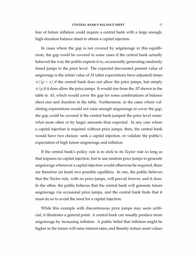
CENTRAL BANK’S BALANCE SHEET 17
fear of future inflation could require a central bank with a large enough,
high-duration balance sheet to obtain a capital injection.
In cases where the gap is not covered by seigniorage in this equilib-
rium, the gap would be covered in some cases if the central bank actually
behaved the way the public expects it to, occasionally generating randomly
timed jumps in the price level. The expected discounted present value of
seignorage is the initial value of M (after expectations have adjusted) times
π/(ρ + x) if the central bank does not allow the price jumps, but simply
π/ρ if it does allow the price jumps. It would rise from the .07 shown in the
table to .43, which would cover the gap for some combinations of balance
sheet size and duration in the table. Furthermore, in the cases where val-
idating expectations would not raise enough seigniorage to cover the gap,
the gap could be covered if the central bank jumped the price level some-
what more often or by larger amounts than expected. In any case where
a capital injection is required without price jumps, then, the central bank
would have two choices: seek a capital injection, or validate the public’s
expectation of high future seigniorage and inflation.
If the central bank’s policy rule is to stick to its Taylor rule so long as
that requires no capital injection, but to use random price jumps to generate
seigniorage whenever a capital injection would otherwise be required, there
are therefore (at least) two possible equilibria. In one, the public believes
that the Taylor rule, with no price jumps, will prevail forever, and it does.
In the other, the public believes that the central bank will generate future
seigniorage via occasional price jumps, and the central bank finds that it
must do so to avoid the need for a capital injection.
While this example with discontinuous price jumps may seem artifi-
cial, it illustrates a general point. A central bank can usually produce more
seigniorage by increasing inflation. A public belief that inflation might be
higher in the future will raise interest rates, and thereby reduce asset values
CENTRAL BANK’S BALANCE SHEET 18
on the central bank’s balance sheet. If the public recognizes that balance
sheet problems might lead the central bank to tolerate higher inflation in or-
der to avoid the need for fiscal support, this can create multiple equilibria.
Different expectations by the public can induce different policy behavior
that validates those expectations.
This simple model has omitted two sources of seigniorage, population
growth and technical progress. It therefore makes it unrealistically easy to
find conditions in which fiscal support is required. The analytic solution for
steady states that we have used for Tables 1 and 2 can be extended to allow
considering more plausible exogenous, non-constant time paths of ρ, x, etc.,
but only with use of numerical integration. Below we expand the model
to include these extra elements and calibrate the parameters and the nature
of the shocks more carefully to the situation of the US Federal Reserve. Of
course our ability to calibrate is limited by the sensitivity of results to the
transactions cost function. We have little relevant historical experience with
currency demand at low or very high interest rates. Rates were very low in
the 1930’s and the early 1950’s, but the technology for making non-currency
transactions is very different now. It is difficult to predict how much and
how fast people would shift toward, say, interest-bearing pre-loaded cash
cards as currency replacements if interest rates increased to historically nor-
mal levels. We can at best show ranges of plausible results.
VI. THE FULL MODEL
Like the simple model, this one borrows from Sims (2005). The house-
hold planner (whose utility includes that of offspring, see Barro and Sala-i
Martin (2004)) maximizes: ∫ ∞
0e−(β−n)t log(Ct)dt (21)
CENTRAL BANK’S BALANCE SHEET 19
where Ct is per capita consumption, β is the discount rate, and n is popula-
tion growth, subject to the budget constraint:
Ct(1 + ψ(vt)) + FPt +
Vt + Mt + qtBP
Pt=
Yeγt + (ρt − n)FPt + (rt − n)
Vt
Pt+ (χ + δ− qtδ− n)
BP
P− n
Mt
Pt− τt. (22)
We express all variables in per-capita terms and initial population is normal-
ized to one. FPt and BP
t are foreign assets and long-term government bonds
in the hand of the public, respectively, Vt denotes central bank reserves, Mt
is currency, τt is lump-sum taxes, Y is an exogenous income stream growing
at rate γ. Foreign assets and central bank reserves pay an exogenous real
return ρ and a nominal return rt, respectively. Long term bonds are mod-
eled as in Woodford (2001). They are assumed to depreciate at rate δ (δ−1
captures the bonds average duration) and pay a nominal coupon χ + δ.6
The government is divided into two distinct agencies called “central
bank” and “fiscal authority”. The central bank’s budget constraint is(qt
BC
Pt− Vt + Mt
Pt
)ent
=
((χ + δ− δqt − nqt)
BC
P− (rt − n)
Vt
Pt+ n
Mt
Pt− τC
t
)ent. (23)
where BCt are long-term government bonds owned by the central bank, and
τCt are remittances from the central bank to the fiscal authority. The central
bank is assumed to follow the rule (5) for setting rt, the interest on reserves.
We also assume that the central bank’s policy in terms of the asset side of
its balance sheet BCt consists in an exogenous process BC
t = BCt . Finally,
the central bank is also assumed to follow a rule for remittances, which we
discuss in section VI.2. We explain there why neither the rule for BCt nor
that for remittances will play a central role in our analysis.
6We write the coupon as χ + δ so that at steady state if χ equals the short term rate the
bonds sell at par (q = 1).
CENTRAL BANK’S BALANCE SHEET 20
Solving the central bank’s budget constraint forward we can obtain its
intertemporal budget constraint:
qBC
0P0− V0
P0+∫ ∞
0(
Mt
Mt+ n)
Mt
Pte−∫ t
0 (ρs+xs−n)dsdt =∫ ∞
0τC
t e−∫ t
0 (ρs+xs−n)dsdt.
(24)
where xs refers to the inflation scare variable discussed in section II (the in-
flation scare results in a premium increasing the real returns on all nominal
assets, and hence enters the central bank’s present discounted value calcula-
tions). Equation (24) shows that, regardless of the rule for remittances, their
discounted present value∫ ∞
0τC
t e−∫ t
0 (ρs+xs−n)dsdt has to equal its left hand
side, namely the market value of assets minus reserves plus the discounted
present value of seigniorage∫ ∞
0(
Mt
Mt+ n)
Mt
Pte−∫ t
0 (ρs+xs−n)dsdt. We can also
compute the constant level of remittances τCeγt (taking productivity growth
into account) that satisfies expression (24).
τC =
(∫ ∞
0e(γ+n)t−
∫ t0 (ρs+xs)dsdt
)−1
(q
Bc
P− V
P+∫ ∞
0(
Mt
Mt+ n)
Mt
Pte−∫ t
0 (ρs+xs−n)dsdt)
. (25)
Government debt is assumed to be held either by the central bank or the
public: Bt = BCt + BP
t . The budget constraint of the fiscal authority is(Gt − τt + (χ + δ− δqt − nqt)
BP
)ent =
(τC
t + qtBPt
)ent, (26)
where Gt is government spending. The rule for τt is given by:
τt = φ0eγt + (φ1 + n + γ)qBP
. (27)
This rule makes the debt to GDP ratio bt = qBP
e−γt converge as long as
φ1 > β− n. The initial level of foreign assets in the hand of the public, cen-
tral bank reserves, and currency are FP0 , V0, and M0, respectively.
CENTRAL BANK’S BALANCE SHEET 21
As in the simple model the first order condition for the household’s
problem with respect to C, FP, B, V, and M yield the Euler equation (13), the
Fisher equation (11),7 the money demand equation (12), and the arbitrage
condition between reserves and long-term bonds:
χ + δ
q− δ +
qq= r. (28)
The solutions for r is given by equation (15), and those for inflationPP
and
velocity v follow from equations (11) and (12), respectively. The growth rate
of consumptionCC
, is given by
CC
= (ρ− β)− 2ψ′(v) + vψ′′(v)1 + ψ(v) + vψ′(v)
v, (29)
which obtains from differentiating expression (13). Differentiating the def-
inition of velocity (3) we obtain an expression for the growth rate of cur-
rency:
MM
=PP+
CC− v
v. (30)
The economy’s resource constraint is given by
C(1 + ψ(v)) + F = (Y− G)eγt + (ρ− n)F, (31)
where F = FP + FC is the aggregate amount of foreign assets held in the
economy (we assume that the central banks foreign reserves FC are zero),
and where we assumed Gt = Geγt. Solving this equation forward we obtain
a solution for consumption in the initial period:
C0
(∫ ∞
0(1 + ψ(v))e−
∫ t0 (ρs− C
C−n)dsdt)= F0 + (Y− g)
∫ ∞
0e(γ+n)t−
∫ t0 ρsdsdt,
(32)
7Note that short term debt was called B in the simple model, and was issued by the
fiscal authority. Here it is called V, and is issued by the central bank.
CENTRAL BANK’S BALANCE SHEET 22
Given velocity v and the level of consumption, we can compute real money
balancesMP
, the initial price level P0, and seigniorageMP
+nMP
=
(MM
+ n)
MP
(using (30)), and the present discounted value of seigniorage
∫ ∞
0
(MM
+ n)
MP
e−∫ t
0 (ρs+xs−n)dsdt = c0
∫ ∞
0
(MM
+ n)
v−1e−∫ t
0 (ρs+xs− CC−n)dsdt.
Finally, solving (28) forward we find the current nominal value of long-term
bonds
q0 = (χ + δ)∫ ∞
0e−(∫ t
0 rsds+δt)
dt. (33)
VI.1. Steady state. At a steady state where ρ = β + γ, r = ρ + π, v satis-
fies v2ψ′(v) = rss. Steady state consumption is given by Ct = C0eγt where
C0 =(β− n)F0 + Y− G
1 + ψ(v), and real money balances are given by
MP ss =
C0
veγt. seigniorage is given by (π + γ + n)
C0
ve(γ+n)t and its present dis-
counted value is given by (π + γ + n)C0
v(β− n).
VI.2. Central bank’s solvency, accounting, and the rule for remittances.
For some of the papers discussed in the introduction the issue of central
bank’s solvency is simply not taken into consideration: the worst that can
happen is that the fiscal authority may face an uneven path of remittances,
with possibly no remittances at all for an extended period. We acknowledge
the possibility that remittances may have to be negative, at least at some
point, if the central bank wants to continue following the interest rate rule:
persisting with its policy rule is impossible without fiscal support from the
Treasury. This is what we mean by “insolvency” for a central bank. It is
important to keep in mind that this notion of solvency depends on what
policy rule the central bank is trying to implement.
Like Reis (2013) and Bassetto and Messer (2013a), we approach the issue
of central bank’s solvency from a present discounted value perspective. If
the left hand side of equation (24) is negative, the central bank cannot face
CENTRAL BANK’S BALANCE SHEET 23
its obligations, i.e., pay back reserves, without the support of the fiscal au-
thority. An interesting aspect of equation (24) is that its left hand side does
not depend on many of aspects of central bank policy that are recurrent in
debates about the fiscal consequences of central bank’s balance sheet policy.
For instance, the future path of BCt does not enter this equation: whether
the central bank holds its assets to maturity or not, for instance, is irrele-
vant from an expected present value perspective. Intuitively, the current
price qt contains all relevant information about the future income from the
asset relative to the opportunity cost rt. Whether the central bank decides
to sell the assets and realize gains or losses, or keep the assets in its port-
folio and finance it via reserves, does not matter. Similarly, whether the
central bank incurs negative income in any given period, and accumulates
a “deferred asset”, is irrelevant from the perspective of the overall present
discounted value of resources transferred to the fiscal authority.8 In fact,
scenarios associated with higher remittances in terms of present value may
well be associated with a deferred asset.
Finally, in perfect foresight the central bank can always choose a per-
fectly smooth path of remittances (in fact, this is τCt = τCeγt). But there are
accounting rules governing central banks’ remittances. Hence these may
not be smooth and may depend on the central bank’s actions, such as hold-
ing the assets to maturity or not. We recognize that the timing of remittances
can matter for a variety of reasons: tax smoothing, political pressures on the
central bank, et cetera. We assume a specific rule for remittances that very
loosely matches those adopted by actual central banks and compute simu-
lated paths of remittances under different assumptions. Since the rule for
8As we will see later central bank accounting does not let negative income affect capital.
The budget constraint (23) implies however that negative income results in either more
liabilities or less assets. To maintain capital nonetheless intact, a “deferred asset” is created
on the asset side of the balance sheet.
CENTRAL BANK’S BALANCE SHEET 24
remittances is not central to our analysis, we leave this discussion to the
appendix.
The rule governing future remittances, for a given amount of central
bank liabilities, does not matter for our results. This is not to say that the
rule for remittances is irrelevant for our discussion of central bank solvency:
the amount of past remittances determines the current level of central bank’s
liabilities, which enter equation (24). Goodfriend (2014) argues that central
banks with large, long-duration balance sheets should retain part of their in-
come in order to build a capital buffer. Such a buffer would be purposeless
if there were explicit fiscal support via an agreement that central bank capi-
tal gains and losses go directly onto the Treasury’s balance sheet9. But in the
absence of such an agreement, a capital buffer could be useful in preserving
central bank independence. Of course time inconsistency of political com-
mitments could undermine either a capital buffer or an explicit agreement
that capital gains and losses go directly to the treasury’s balance sheet. A
capital buffer could become a political target if perceived as unnecessarily
large; an explicit agreement might work well while capital gains were flow-
ing to the treasury, but be called into question when it started requiring
flows in the reverse direction.
VI.3. Functional forms and parameters. Table 3 shows the model parame-
ters. We normalize Y− g to be equal to 1, and set F0 to 0.10 Since we do not
have investment in our model, and F0 = 0, Y− G in the model corresponds
to national income Y minus government spending G in the data (data are
from Haver analytics, mnemonics are Y@USNA and G@USNA, respectively).
9The Bank of England has such an accounting arrangement with the Treasury (McLaren
and Smith, 2013).10Note from the steady state calculations that we could choose F0 6= 0 and use instead
the normalization (β − n)F0 + y − g=1, hence setting F0 6= 0 simply implies a different
normalization.
CENTRAL BANK’S BALANCE SHEET 25
All real quantities discussed in the remainder of the paper should therefore
be understood as multiples of Y− G, and their data counterparts are going
to be expressed as a fraction of national income minus government spend-
ing ($ 11492 bn in 2013Q3). Our t = 0 corresponds to the beginning of 2014.
We therefore measure our starting values for the face value of central bank
assetsBC
P, reserves
VP
, and currencyMP
using the January 2, 2014 H.4.1 re-
port (http://www.federalreserve.gov/releases/h41/), which mea-
sures the Security Open Market Account (SOMA) assets.11 We choose χ –
the average coupon on the central bank’s assets – to be 3.4 percent, roughly
in line with the numbers reported in figure 6 of Carpenter, Ihrig, Klee,
Quinn, and Boote (2013). Chart 17 of the April 2013 FRBNY report on “Do-
mestic Open Market Operations during 2013”12 shows an average duration
of 6.8 years for SOMA assets (SOMA is the System Open Market Account,
which represents the vast majority of the Federal Reserve balance sheet).
Accordingly we set 1/δ =6.8.
11The January 2, 2014, H.4.1 reports the face value of Treasury ($ 2208.791 bn ), GSE debt
securities ($ 57.221 bn), and Federal Agency and GSE MBS ($ 1490.160 bn), implying that
BC0 is $ 3756.172 bn, the value of reserves and other interest-bearing central bank liabilities
V (these include reserve balances for $ 2374.633 bn and reverse repurchase agreements for $
235.086 bn) and currency M (Federal Reserve currency in circulation $ 1240.499 bn) on Jan-
uary 1, 2014. Note that while our description of the central bank’s balance sheet is coarse,
we are not missing any quantitatively important item. Our measure of B includes the total-
ity of “Securities held outright”. We are missing “Unamortized premiums /discounts,” but
that is an accounting measure of qB− B, so it is appropriate not to include this item. We
are also missing discount window and other credit, gold, foreign currency denominated
assets, and Treasury currency on the asset side. Relative to the overall size of the balance
sheet, these items are quite small. On the liability side we are missing Treasury cash hold-
ings, “deposits with F.R. Banks, other than reserve balances,” which is mostly comprised of
the U.S. Treasury general account and other non-interest bearing liabilities. “Term deposits
held by depository institutions” are interest bearing and ought to be included in V, but
were zero on January 1, 2014.12http://www.newyorkfed.org/markets/omo/omo2013.pdf.
The remaining model parameters are chosen as follows. The discount
rate β, productivity growth γ, and population growth n are 1 percent, 1
percent, and .75 percent, respectively. These values are consistent with Car-
penter et al.’s assumptions of a 2% steady state real rate.
The policy rule has inflation and interest rate smoothing coefficients θπ
and θr of 2 and 1, respectively, which are roughly consistent with those of in-
terest feedback rules in estimated DSGE models (e.g., Del Negro, Schorfheide,
Smets, and Wouters (2007); note that θr = 1 corresponds to an interest rate
smoothing coefficient of .78 for a policy rule estimated with quarterly data).
The inflation target θπ is 2 percent. As in the simple model, we use for
transactions costs the functional form (20), which we repeat here for conve-
nience:
ψ(v) = ψ0e−ψ1/v . (20)
This transaction cost function implies that the elasticity of money demand
goes to zero for very low interest rates, consistently with the evidence in
Mulligan and Sala-i Martin (2000) and Alvarez and Lippi (2009). The co-
efficients ψ0 and ψ1 used in the baseline calibration are ψ0 =.63 and ψ1 =
103.14. These were obtained from an OLS regression of log r on inverse
velocity, which is justified by the fact that under this functional form for the
transaction costs the equilibrium condition (12) implies
log r = log(ψ0ψ1)− ψ1v−1. (34)
The left panel of Figure 1 shows the scatter plot of quarterlyMPC
= v−1
and the annualized 3-month TBill rate in the data (where M is currency and
PC is measured by nominal PCE)13, where black crosses are post-1959 data,
13Data are from Haver, with mnemonics C@USNA, FMCN@USECON, and FTBS3@USECON
for PCE, currency, and the Tbill rate, respectively.
CENTRAL BANK’S BALANCE SHEET 27
FIGURE 1. Money Demand and the Laffer CurveShort term interest rates and M/PC Laffer Curve
0 0.05 0.1 0.15 0.20.04
0.06
0.08
0.1
0.12
0.14
0.16
0.18
M/P
C
r
2013
2008
Model
pre 1959 data
post 1959 data
0 0.2 0.4 0.6 0.8 1 1.2 1.4 1.6 1.8 2−0.01
0
0.01
0.02
0.03
0.04
0.05
0.06
0.07
Se
ign
iora
ge
piss
Notes: The left panel shows a scatter plot of quarterlyMPC
= v−1 and the annualized 3-month TBill
rate (black crosses are post-1959 data, and gray crosses are 1947-1959 data) together withrelationship between inverse velocity and the level of interest rates implied by the model (solidblack line). The right panel shows seigniorage as a function of steady state inflation.
and gray crosses are 1947-1959 data, which we exclude from the estima-
tion as they represent an earlier low-interest rate period where the trans-
action technology was arguably quite different. The solid black curve in
the left panel of Figure 1 shows the relationship between inverse velocity
and the level of interest rates implied by the model.14 The right panel of
Figure 1 shows the steady state Laffer curve as a function of inflation. The
figure shows that under our parameterization seigniorage is still increas-
ing even for inflation rates of 200 percent (eventually money demand and
seigniorage go to zero, but this only occurs for interest rates above 6500 per-
cent). We also consider alternative parameterizations of currency demand.
Specifically, we run the OLS regression excluding post-2008 data and obtain
a substantially lower estimate of ψ1, implying a greater sensitivity of money
demand to interest rates (ψ1= 48.17, ψ0 = .03). Figure A-1 in the appendix
14The implied transaction costs at steady state are negligible - about .04 percent of Y-G.
CENTRAL BANK’S BALANCE SHEET 28
shows that the Laffer curve under this parameterization appears very dif-
ferent from that in Figure 1, with the Laffer curve peaking at 50 percent
interest rates, and money demand going to zero for r above 150 percent.
As we discuss later, our quantitative results do not change much depend-
ing on which parameterization of the currency demand function we use.
Nonetheless, we acknowledge there is much uncertainty regarding future
currency demand as new technologies and alternative means of payments
(e.g., interest-bearing cash cards) may change it substantially. This implies
that much uncertainty surrounds our quantitative findings.
TABLE 3. Parameters
normalization, foreign assets
Y− G = 1 F0 = 0
initial assets, reserves, and currencyBC
P= 0.323
VP
= 0.224MP
= 0.107
bonds: duration and coupon
δ−1 = 6.8 χ = 0.034
discount rate, reversion to st.st., population and productivity growth
β = 0.01 γ = 0.01
ϕ1 = 0.750 n = 0.0075
monetary policy
θπ = 2 θr = 1
π = 0.02
money demand
ψ0 = 0.63 ψ1 = 103.14
CENTRAL BANK’S BALANCE SHEET 29
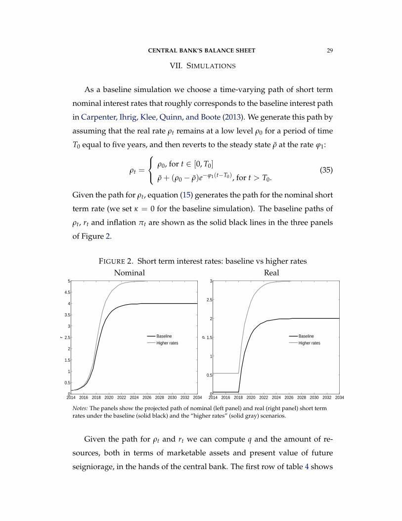
VII. SIMULATIONS
As a baseline simulation we choose a time-varying path of short term
nominal interest rates that roughly corresponds to the baseline interest path
in Carpenter, Ihrig, Klee, Quinn, and Boote (2013). We generate this path by
assuming that the real rate ρt remains at a low level ρ0 for a period of time
T0 equal to five years, and then reverts to the steady state ρ at the rate ϕ1:
ρt =
ρ0, for t ∈ [0, T0]
ρ + (ρ0 − ρ)e−ϕ1(t−T0), for t > T0.(35)
Given the path for ρt, equation (15) generates the path for the nominal short
term rate (we set κ = 0 for the baseline simulation). The baseline paths of
ρt, rt and inflation πt are shown as the solid black lines in the three panels
of Figure 2.
FIGURE 2. Short term interest rates: baseline vs higher ratesNominal Real
Notes: The panels show the projected path of nominal (left panel) and real (right panel) short termrates under the baseline (solid black) and the “higher rates” (solid gray) scenarios.
Given the path for ρt and rt we can compute q and the amount of re-
sources, both in terms of marketable assets and present value of future
seigniorage, in the hands of the central bank. The first row of table 4 shows
CENTRAL BANK’S BALANCE SHEET 30
the two components of the left hand side of equation (24), namely the mar-
ket value of assets minus reserves (column 1) and the discounted present
value of seigniorage∫ ∞
0(
MM
+ n)MP
e∫ t
0 (ρs+xs−n)dsdt (column 2). The third
column shows the sum of the two, which has to equal the discounted present
value of remittances∫ ∞
0τCe
∫ t0 (ρs+xs−n)dsdt. Last, in order to provide in-
formation about how the numbers in column 1 are constructed, column 4
shows the nominal price of long term bonds q at time 0.
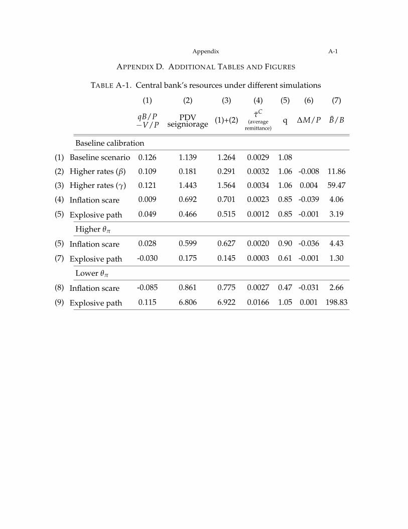
TABLE 4. Central bank’s resources under different simulations(1) (2) (3) (4) (5)
qB/P−V/P
PDVseigniorage (1)+(2) q B/B
Baseline calibration
(1) Baseline scenario 0.126 1.139 1.264 1.08
(2) Higher rates (β) 0.109 0.181 0.291 1.06 11.86
(3) Higher rates (γ) 0.121 1.443 1.564 1.06 59.47
(4) Inflation scare 0.009 0.692 0.701 0.85 4.06
(5) Explosive path 0.049 0.466 0.515 0.85 3.19
Higher θπ
(6) Inflation scare 0.028 0.599 0.627 0.90 4.43
(7) Explosive path -0.030 0.175 0.145 0.61 1.30
Lower θπ
(8) Inflation scare -0.085 0.861 0.775 0.47 2.66
(9) Explosive path 0.115 6.806 6.922 1.05 198.83
Notes: The table shows the two components of the left hand side of equation (24), namely the marketvalue of assets minus reserves (column 1) and the discounted present value of seigniorage (column2). Column 3 shows the sum of the two, which has to equal the discounted present value ofremittances. Column 4 shows the nominal price of long term bonds q at time 0. Column 5 reportsfor each scenario the level of the balance sheet BC (expressed as a fraction of the end-of-2013 level)such that, for any balance sheet size larger than BC, the present discounted value of remittancesbecomes negative after the shock.
CENTRAL BANK’S BALANCE SHEET 31
Under the baseline simulation the real value of the central bank’s assets
minus liabilities is 12.6 percent of Y-G – which is larger than the difference
between the par value of assets minus reserves reported in table 3 given that
q is above one under the baseline. Its value is 1.08, which is above the 1.04
ratio of market over par value of assets reported in Federal Reserve System
(2014).15 The discounted present value of seigniorage is almost an order of
magnitude larger, however, at 114 percent of Y-G, and represents the bulk
of the central bank resources (and therefore of the present discounted value
of remittances), which are 126 percent of Y-G.16
Note that our estimate of the present discounted value of seigniorage is
quite large. A look at the steady state formula for the PDV of seigniorage
provided in section VI explains why this is the case. The numerator in that
formula – the flow of seigniorage – is (π + γ + n) m, where m is real money
balances. Our calibration implies that this flow is .0027 of Y-G, lower than
the historical average seigniorage (.0047). The reason why our present dis-
counted value is so large is that the denominator β− n is very small. This
also implies that the present discounted value numbers are very sensitive
to the calibration of the discount rate, as we show below.
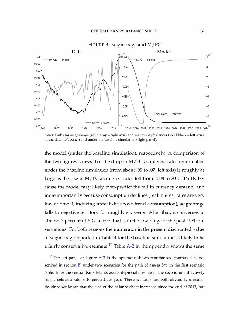
The left and right panels of Figures 3 show inverse velocity M/PC and
seigniorage, expressed as a fraction of Y-G, in the data (1980-2013) and in
15Page 23 and 29 shows the par and market (fair) value of Treasury and GSE debt secu-
rities, and Federal Agency and GSE MBS, respectively.16Column 4 in Table A-1 in the appendix shows τC as defined in equation (25): the
constant level of remittances (accounting for the trend in productivity) that would satisfy
equation (24), expressed as a fraction of Y-G like all other real variables. That is, the amount
τC such that τCt = τCeγt satisfies the present value relationship. We find that the constant
(in productivity units) level of remittances τC that satisfies the present value relationship
is .29 percent of Y-G, about $ 34 bn per year, considerably lower than the amount remit-
ted for 2013 and 2012 according to Federal Reserve System (2014) ($ 79.6 and $ 88.4 bn,
Notes: Paths for seigniorage (solid gray – right axis) and real money balances (solid black – left axis)in the data (left panel) and under the baseline simulation (right panel).
the model (under the baseline simulation), respectively. A comparison of
the two figures shows that the drop in M/PC as interest rates renormalize
under the baseline simulation (from about .09 to .07, left axis) is roughly as
large as the rise in M/PC as interest rates fell from 2008 to 2013. Partly be-
cause the model may likely over-predict the fall in currency demand, and
more importantly because consumption declines (real interest rates are very
low at time 0, inducing unrealistic above trend consumption), seigniorage
falls to negative territory for roughly six years. After that, it converges to
almost .3 percent of Y-G, a level that is in the low range of the post-1980 ob-
servations. For both reasons the numerator in the present discounted value
of seigniorage reported in Table 4 for the baseline simulation is likely to be
a fairly conservative estimate.17 Table A-2 in the appendix shows the same
17The left panel of Figure A-3 in the appendix shows remittances (computed as de-
scribed in section B) under two scenarios for the path of assets BC: in the first scenario
(solid line) the central bank lets its assets depreciate, while in the second one it actively
sells assets at a rate of 20 percent per year. These scenarios are both obviously unrealis-
tic, since we know that the size of the balance sheet increased since the end of 2013, but
CENTRAL BANK’S BALANCE SHEET 33
quantities of Table 4 obtained under the alternative calibration of money
demand. We see that in spite of the differences in the elasticity, the results
in terms of central bank’s resources are very similar.
Next, we consider alternative simulations where the economy is sub-
ject to different “shocks.” In each of these simulations all uncertainty is
revealed at time 0, at which point the private sector will change its con-
sumption and portfolio decisions and prices will adjust. We will use the
subscript 0− to refer to the pre-shock quantities and prices (that is, the time
0 quantities and prices under the baseline simulation). For each simula-
tion, Table 4 will report the new market value of assets minus reserves in
real term (q0BC
0−
P0− V0
P0). By assumption the central bank will not change
its assets BC0− after the new information is revealed, but the private sector
will change its time 0 currency holdings given that interest rates may have
changed. This necessarily leads to a change in reserves (given that central
bank’s assets are unchanged) equal to
V0 −V0−
P0= −M0 −M0−
P0, (36)
in real terms (we report this quantity in column 6 of Table A-1 in the appen-
dix).
For each scenario we also report the level of the balance sheet BC such
that, for any balance sheet size larger than BC, the present discounted value
of remittances (see equation (24)) becomes negative after the shock. We refer
to this situation as the central bank becoming “insolvent”, in the sense that
it needs resources from the fiscal authority because it suffered losses due to
the fall in q. Specifically, assume the central bank expands its balance sheet
by ∆BC at time 0− (right before the shock takes place) by buying assets at
highlight the fact that different paths for the balance sheet can imply different paths for
remittances, even though their expected present value remains the same (this is the dotted
line in Figure A-3, which shows τCeγt).
CENTRAL BANK’S BALANCE SHEET 34
price q0− and pays for its purchases by expanding reserves by an amount
∆V = q0−∆BC. How large can ∆BC be to still satisfy
q0(
BC + ∆BC)−V − ∆VP0
+M0 −M0−
P0+∫ ∞
0(
Mt
Mt+ n)
Mt
Pte−∫ t
0 (ρs+xs−n)dsdt ≥ 0 (37)
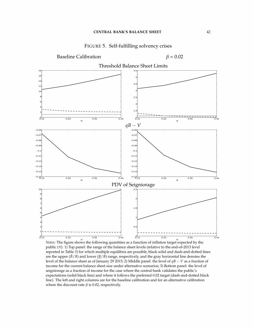
after the “shock”? Column 5 of Table 4 reports B/BC = 1 +∆BC
BC , where BC
is the 2013Q4 level of the balance sheet reported in Table 3.
The first alternative scenario we study is a “higher rates” path similar to
one considered by Carpenter, Ihrig, Klee, Quinn, and Boote (2013). Under
this new path real rates converge to a 1 percent higher steady state, and so
will short term nominal rates given that the central bank inflation target has
not changed. We choose the new starting value for ρ, ρ0, so that the initial
rate remains at 13.5 basis points. The gray solid lines in the two panels of
Figure 2 show the “Higher Rates” paths for the nominal and the real short
term rates, respectively. In these simulations we assume that the central
bank recognizes the change in the steady state ρ = β + γ, and adjusts its
Taylor rule coefficient r = ρ + π accordingly.
We consider two different reasons why the new steady state ρ is higher:
a higher discount rate β and a higher growth rate of technology γ. While
the new value of q is the same in both cases (the interest rate path is the
same), the present value of seigniorage shown in column 2, and therefore
the present value of remittances shown in column 3, is quite different. In
the high β case the current value of the future income from seigniorage falls
by almost one order of magnitude, as future seigniorage is discounted at
a higher real rate. In the high γ case the economy is growing faster, and
so does money demand and future seigniorage. Table A-1 in the appendix
shows that in both cases (higher β and higher γ) the level of τC is higher
than in the baseline case. Carpenter, Ihrig, Klee, Quinn, and Boote (2013)
CENTRAL BANK’S BALANCE SHEET 35
take seigniorage as given and focus on the effect of the higher nominal inter-
est rates on the value of the central bank’s assets qBC, which falls following
the drop in q. The effect of the higher real rate of return on future central
bank’s revenues and, especially in the high γ case, on future seigniorage,
trumps in our simulation the negative effect on q. 18
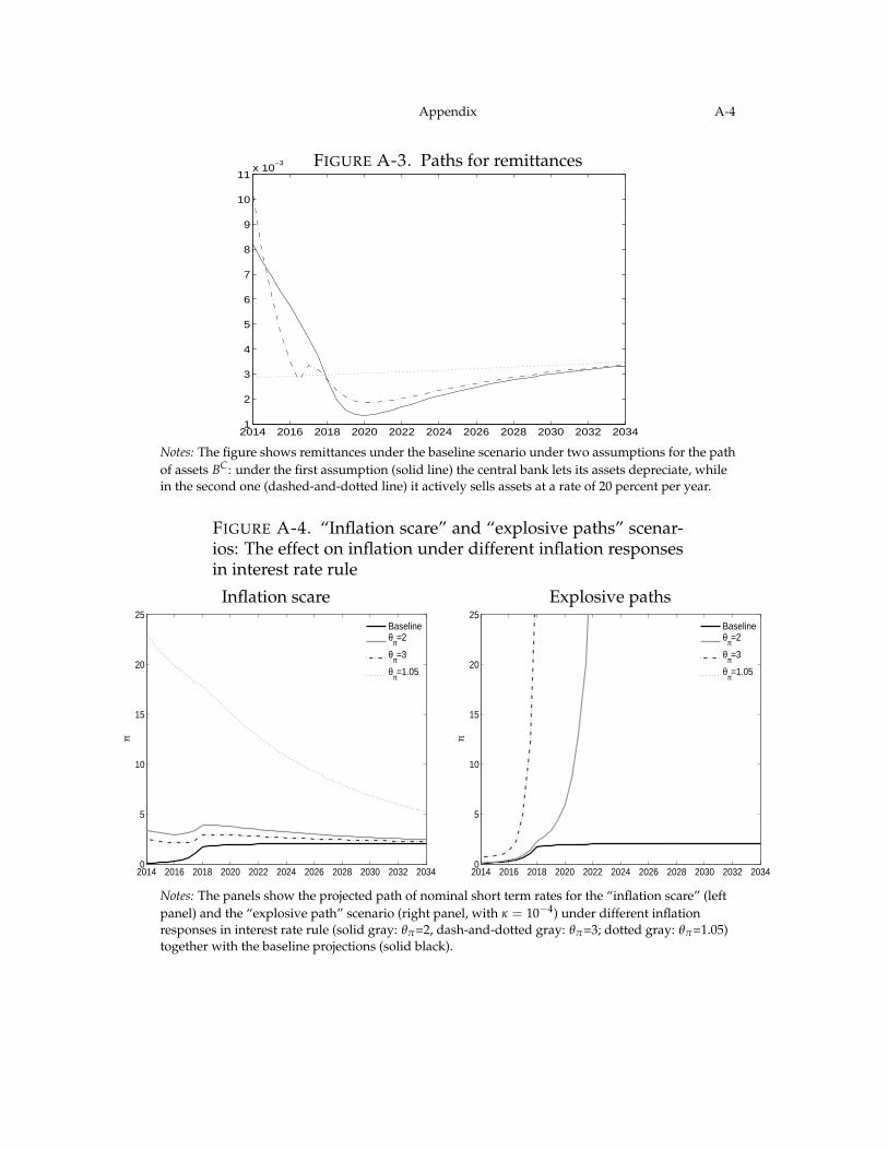
FIGURE 4. “Inflation scare” and “explosive paths” scenarios:The effect on short terms rates under different inflation re-sponses in interest rate rule
Notes: The panels show the projected path of nominal short term rates for the “inflation scare” (leftpanel) and the “explosive path” scenario (right panel, with κ = 10−4) under different inflationresponses in interest rate rule (solid gray: θπ=2, dash-and-dotted gray: θπ=3; dotted gray: θπ=1.05)together with the baseline projections (solid black).
Next, we consider simulations where the private sector is concerned
about a sudden jump in the price level, and therefore demands a premium
xt for holding nominal bonds as described in section II (“inflation scares”
scenarios). We assume that this premium follows the process
xt = x0e−χxt, (38)
18This may seem surprising in the higher β case since the present value of seigniorage
is lower than under the baseline simulation. However, the central bank is now earning a
higher return on its assets, and can therefore afford a higher level of remittances.
CENTRAL BANK’S BALANCE SHEET 36
with x0 = .04 and χx = .1. The solid gray line in the left panel of Figure 4
shows the path of the short term nominal interest rates under this scenario,
which is higher than under the baseline because the higher inflation expec-
tations force the central bank to raise rates (the corresponding paths for in-
flation are shown in Figure A-4 in the appendix). Row 4 of Table 4 shows the
effects of this scenario on the central bank’s balance sheet. The market value
of assets minus reserves q0BC
0−
P0− V0
P0drops to almost zero, both because q
falls and because a higher fraction of the central bank’s liabilities becomes
interest bearing relative to the baseline scenario. This happens because the
private sector turns currency into reserves, driven by the higher opportu-
nity cost of holding currency. Under our assumptions on money demand,
the present discounted value of seigniorage, while lower than in the base-
line case, is still sizable, and so is the present value of resources in the hands
of the central bank under this scenario. As a consequence, even with a much
larger balances sheet (more than four times as large) the central bank could
have withstood the fall in the value of its assets without ever needing any
resources from Fiscal Authority. Table A-2 in the appendix shows that these
results are robust to the parameterization of money demand.
The quantitative results are sensitive to the inflation response in the pol-
icy reaction function. The dash-and-dotted and dotted gray lines in the left
panel of Figure 4 show the interest rate path corresponding to an inflation
coefficient θπ of 3 and 1.05, respectively.19 As is usually the case in stable
rational expectations equilibria, a higher inflation coefficient in the interest
rate rule induces a lower equilibrium response of inflation, and therefore
a lower equilibrium response of interest rates – and vice versa when the
inflation response is lower. When θπ is 1.05, interest rates reach almost 30
19In these simulations we change the time 0 real rate so that under the baseline scenario
the nominal rate is still 13.5 basis points.
CENTRAL BANK’S BALANCE SHEET 37
percent. Consequently, q falls to less than half its value in the baseline sce-
nario, and the market value of assets minus reserves q0BC
0−
P0− V0
P0falls to
negative levels (see row 8 of Table 4). The implication of this finding is that
under a large balance sheet the central bank may want to respond more ag-
gressively to inflation if it is concerned about fluctuations in the values of
its assets.
Even in the θπ = 1.05 case central bank’s solvency is not an issue, how-
ever. The central bank’s overall resources (column 3) are still sizable, be-
cause the higher inflation experienced under the lower θπ policy yields
greater seigniorage (column 2). In fact, the present value of remittances
would remain positive even if we assumed the central bank balance sheet
to be more than twice as large as the current one (column 5).
Finally, we consider explosive paths where κ in equation (15) is different
from zero. The solid gray line in the bottom right panel of Figure 4 shows
one of these paths (with κ = 10−4) under the baseline policy response.
Given the rise in rt under this scenario, q drops substantially relative to
the baseline (row 5 of Table 4). The present discounted value of seigniorage
also falls relative to the baseline because seigniorage goes to zero as rates
become larger than 6500 percent. But it is still large enough that even with
a balance sheet more than three times as large as Bc0 the central bank would
be solvent. This is one case where using the alternative parameterization
of money demand makes a difference, however. Table A-2 in the appendix
shows that under explosive paths the central bank would not be solvent un-
der the current size of the balance sheet, which is not surprising since under
this parameterization the peak of the Laffer curve is crossed at interest rates
around 50 percent.
The dash-and-dotted and dotted gray lines in the bottom right panel
of Figure 4 show the responses under different θπ coefficients. In the case
of unstable solutions, the inflation response coefficient in the interest rule
CENTRAL BANK’S BALANCE SHEET 38
plays the opposite role relative to the stable solution case (see Cochrane
(2011)): the stronger the response, the faster inflation and interest rates ex-
plode. The market value of central bank’s assets q surely falls more with a
higher θπ, and indeed q0BC
0−
P0− V0
P0falls to negative levels. The present dis-
counted value of seigniorage also falls by more than in the θπ = 2 case, but
not by enough to call central bank’s solvency in question under these paths.
VIII. SELF-FULFILLING SOLVENCY CRISES
As we have already observed, a central bank cannot guarantee determi-
nacy of the price level in the absence of fiscal backing. Our detailed scenar-
ios in the previous sections have all assumed (except in the κ > 0 cases) that
this backing was present. But even when the backing is present, a central
bank that is firmly committed to not accepting (or incapable of drawing on)
fiscal support, in the sense of capital injections from the treasury, can create
indeterminacy in the price level.
What if the public believes that, were the central bank to face the issue of
solvency, it would resort to seigniorage creation? Entertaining this possibil-
ity would then lead the public to expect higher future inflation and nominal
interest rates. These expectations would result in a lower value of long term
nominal assets today, so that the central bank’s assets qBC could become
worth less than its interest bearing liabilities V. If the current present dis-
counted value of seigniorage is not large enough to cover this gap, the cen-
tral bank might have to resort to raising more seigniorage, thereby validat-
ing the initial belief. The larger is the size of the central bank’s balance sheet,
and the longer its duration, the larger is the gap in qBC−V that would arise
CENTRAL BANK’S BALANCE SHEET 39
because of future expected inflation, and the higher the likelihood of these
alternative equilibria.20
We make this point more formally by focusing on a simple setting. We
assume that the central bank chooses at time 0 the inflation target π in its
Taylor rule (5) and would like to set it to 2 percent. In choosing π, we
assume that the central bank is constrained by the lack of fiscal support –
hence τCt ≥ 0 in all future periods t ≥ 0, implying that the left hand side of
the intertemporal constraint (24) must be non-negative for all t ≥ 0 – and
by the equilibrium conditions (11), (12), (24), (29), (30), (32), (33).
We have already verified that if the central bank chooses a target of 2
percent for all periods (πt = .02) and the public’s expectations align with
this choice, the central bank solvency constraint is slack (see Table 1). This
is therefore an equilibrium, as it satisfies the central bank’s objective and all
the constraints. But there may be other equilibria where the public instead
believes that the central bank will be forced by balance sheet considerations
to push inflation, and thus seigniorage, higher. In these equilibria the level
of π is π > .02 and the solvency constraint is satisfied:
q0(π)BC0− −V0(π)
P0(π)+ PDVS0(π) ≥ 0, (39)
20There is a connection between self-fulfilling equilibria in this paper and the literature
on currency crisis (e.g., Burnside, Eichenbaum, and Rebelo (2004)) and debt crisis (espe-
cially Calvo (1988)). In Burnside, Eichenbaum, and Rebelo (2004), government guarantees
lead to the possibility of self- fulfilling speculative attack on the exchange rate regime.
In this paper, the presence of long-duration assets in the central bank’s balance sheet
makes it vulnerable to expectations of higher future inflation, and the lack of fiscal support
makes these expectations self-fulfilling because it has to resort to seigniorage. Similarly, a
large, long-duration balance sheet in this model plays the same role as a large outstanding
amount of debt in Calvo, in that it “may generate the seeds of indeterminacy; it may, in
other words, generate a situation in which the effects of policy are at the mercy of people’s
expectations ... ”(Calvo (1988), pg. 648).
CENTRAL BANK’S BALANCE SHEET 40
where q0(π), P0(π), V0(π), and PDVS0(π) =∫ ∞
0(
Mt
Mt+n)
Mt
Pte−∫ t
0 (ρs−n)dsdt
are the time 0 asset price, price level, reserves, and present discounted value
of seigniorage, respectively, implied by the inflation target π.21 Values of π
for which equation (39) is satisfied are possible self-fulfilling solvency crises,
in the sense that the expectation that the central bank will switch to a new
rule with target π will produce a gap in the value of central bank’s assets
minus liabilitiesq0(π)BC
0− −V0
P0(π)that will be filled with future seigniorage
PDVS0(π).
To keep the analysis of the equilibrium simple, suppose that the public
expects the central bank to follow a Taylor rule with either π = .02 or π = π.
If 1) condition (39) is satisfied, and 2) with π at the desired .02 level instead
of π condition (39) is not satisfied, then there are two possible equilibria.
The public may believe the higher value of π is likely, in which case the
central bank must set π = π to avoid the need for a capital injection, as we
show in appendix C; or the public may believe that the π = .02 equilibrium
will prevail, in which case it does.22
If the size of the balance sheet BC0 is at a level B(π) that makes (39) hold
with equality when the public expects a target π, then the conditions for
multiplicity are certainly met. However, even for a slightly smaller size
of the balance sheet pursuing a π = .02 policy may not generate enough
seigniorage if the public expects π = π. This is because the difference be-
tween PDVS0(π) and the seigniorage generated under the deviation π =
21As mentioned in the discussion of equation (36), V0 differs from the initial level of
reserves V0− because of time 0 changes in currency demand.22It may seem contradictory to suppose that, if the policy authority sticks to π = .02,
expected inflation remains on the higher path. If the public thinks of the higher inflation
as being generated by randomly timed neutral jumps in M and P (as in our inflation scare
example of Section II), however, there is no clear irrationality in their maintaining high
.02 is large enough to overwhelm the reduction in the gap V0 − q0BC0 aris-
ing from a smaller balance sheet BC0 .23 Below some level B(π) high infla-
tion expectations are no longer self-fulfilling. The central bank can avoid a
capital injection despite the high inflation expectations, even if it maintains
π = .02, and the public will have no reason to believe that π = π will be
forced by a need to avoid a capital injection.
Whether multiple equilibria are possible depends on the level (and du-
ration) of the balance sheet. The top two panels in Figure 5 show, as a func-
tion of π, the range of initial balance sheet values (B, B) for which multiple
equilibria are possible. The left and right panels are for the baseline cali-
bration and for an alternative calibration where the discount rate β is 0.02,
respectively. The figure shows that under the baseline money demand cali-
bration, the upper, B balance sheet level is in all cases much larger than the
end-of-2013 one (B/B > 1), and also larger than the level of the balance sheet
reached on January 29 2015 (this is $ 4244 bn, or 13 percent higher than the
end-of-2013 level, and is shown by a gray horizontal line). The lower end of
the range comes much closer to the January 2015 level of the balance sheet,
though, and indeed goes below it for the β = .02 case at very high π lev-
els. At levels of initial balance sheet below B but above B, seigniorage more
than covers the initial capital loss, and at the low end of the range, with B
23It is important that we have considered π and 2 percent as the only two choices of
the central bank. If we allow the central bank to entertain any response π ∈ [.02 π], then
they would choose the lowest π satisfying condition (39) with equality. We would still
have two possible equilibria, but in this case, unless eqrefeq:mul held with equality at
π = π, the higher-inflation equilibrium would have actual π below its expected value π
and would therefore not be a self-confirming equilibrium. A more sophisiticated analysis
would credit the public with the ability to learn by observing central bank behavior and
credit the central bank with the ability to choose time varying as well as constant paths
for π, or even to revert to passive monetary policy. We leave a deeper analysis to future
research.
CENTRAL BANK’S BALANCE SHEET 42
FIGURE 5. Self-fulfilling solvency crises
Baseline Calibration β = 0.02
Threshold Balance Sheet Limits
0.15 0.25 0.35 0.450
2
4
6
8
10
12
14
16
18
π0.15 0.25 0.35 0.451
1.5
2
2.5
3
3.5
4
4.5
π
qB−V
0.15 0.25 0.35 0.45−0.15
−0.14
−0.13
−0.12
−0.11
−0.1
−0.09
−0.08
−0.07
−0.06
π0.15 0.25 0.35 0.45
−0.15
−0.14
−0.13
−0.12
−0.11
−0.1
−0.09
−0.08
−0.07
−0.06
π
PDV of Seigniorage
0.15 0.25 0.35 0.450
1
2
3
4
5
6
7
8
9
10
π0.15 0.25 0.35 0.450
0.5
1
1.5
2
2.5
πNotes: The figure shows the following quantities as a function of inflation target expected by thepublic (π): 1) Top panel: the range of the balance sheet levels (relative to the end-of-2013 levelreported in Table 3) for which multiple equilibria are possible; black solid and dash-and-dotted linesare the upper (B/B) and lower (B/B) range, respectively, and the gray horizontal line denotes thelevel of the balance sheet as of January 29 2015; 2) Middle panel: the level of qB−V as a fraction ofincome for the current balance sheet size under alternative scenarios; 3) Bottom panel: the level ofseigniorage as a fraction of income for the case where the central bank validates the public’sexpectations (solid black line) and where it follows the preferred 0.02 target (dash-and-dotted blackline). The left and right columns are for the baseline calibration and for an alternative calibrationwhere the discount rate β is 0.02, respectively.
CENTRAL BANK’S BALANCE SHEET 43
just above B, the seigniorage in the high-inflation equilibrium is so far in
excess of what is needed that such equilibria are implausible.
The middle panel shows what happens toq0(π)BC
0− −V0
P0(π)in the alter-
native equilibrium under the current balance sheet size. The baseline case
(left) column of the figure shows that for π greater than 15 percent the real
value of assets minus interest bearing liabilities does become negative. The
solid black line in the bottom panel of Figure 5 shows that for these val-
ues the level of seigniorage PDVS0(π) overshadows this balance sheet loss:
the increase in seigniorage triggered by the higher inflation regime is larger
than the balance sheet loss caused by the fall in q.24 Hence the results in the
top left panel: the size of the balance sheet would have to be much larger
than the current one for the balance sheet loss to be of the same size of the
increase in seigniorage.
The middle plot in the right-hand column of the figure shows that with
a higher real rate, the initial capital loss in the high-inflation equilibrium is
about the same order of magnitude as in the base case. But the bottom right
plot shows, via the vertical axis labels, that seigniorage is much lower in this
case, which is why we saw in the top right graph that multiple equilibria
could occur at the January 2015 level of the balance sheet, at very high levels
of inflation and at the lower end of the (B, B) range.
Though this example shows multiple equilibria are in principle possi-
ble, it does not generate convincing examples of multiple equilibria at or
near current levels of the Fed balance sheet. We should bear in mind, how-
ever, that these results are sensitive to parameter values within reasonable
ranges, as shown by the contrast between the two columns of Figure 5.
In addition, including features that are absent in this simple model, such
24The Laffer curve in the right panel of Figure 1 shows why the increase in seigniorage
is so large under the baseline parameterization of money demand: even for large interest
rates seigniorage grows almost linearly with inflation.
CENTRAL BANK’S BALANCE SHEET 44
as variations in term premia, could change the quantitative results signifi-
cantly. 25
The multiplicity considered in this section can be eliminated with fiscal
support for the central bank’s balance sheet such as the arrangement be-
tween the Bank of England and Her Majesty’s Treasury, whereby all gains
and losses incurred by the former as part of its asset purchase facility are
transfered to the latter (see McLaren and Smith (2013)). In this model,
the mere presence of fiscal support eliminates the multiplicity, without any
need for actual support in equilibrium.
IX. CONCLUSIONS
The large balance sheet of many central banks has raised concerns that
they could suffer significant losses if interest rates rose, and might need a
capital injection from the fiscal authority. This paper constructs a simple
deterministic general equilibrium model, calibrated to US data, to study
the the impact of alternative interest rates scenarios on the central bank’s
balance sheet.
One fundamental point that the model illustrates is that concerns about
the central bank balance sheet are distinct from concerns about whether
fiscal policy is such as to guarantee a determinate price level. The literature
on the fiscal theory of the price level studies mutual constraints on fiscal
25Figure A-5 in the appendix shows that multiple equilibria may rise under the current
balance sheet level if expectations about future seigniorage change dramatically relative to
the baseline. There, we explore multiple equilibria in the situation where we consider non
stationary solutions to equation (15): in these simulations, κ <0 implies that the interest rate
is bound to eventually hit the lower limit r and to remain there forever after (in absence
of the appropriate fiscal policies alluded to in section III; we choose κ so that the ZLB
is hit again after 3.5 years). Under many of these paths the present discounted value of
seigniorage is no longer enough to compensate for the decline in the value of the central
bank assets.
CENTRAL BANK’S BALANCE SHEET 45
and monetary policy required to guarantee a determinate price level. That
kind of fiscal-monetary policy interaction, which we call fiscal “backing”, is
distinct from the within-government transfers between the treasury and the
central bank that are the main focus of this paper, and that we label fiscal
“support”. Most of our analysis simply assumes fiscal backing, though we
do show that the absence of fiscal backing (κ 6= 0 solutions) can make a
dramatic difference to our simulations and calculations of the need for fiscal
support.26
Assuming fiscal backing, we show that the central bank’s policy rule
(or, equivalently, inflation objectives), and the behavior of seigniorage un-
der high inflation are crucial in determining whether a capital injection —
i.e. fiscal support — might be needed. We show also that a central bank
that is seen as ready, in order to avoid a need for capital injection, to cre-
ate seignorage by altering its inflation objectives, can thereby lose control
of the price level, even where with a different policy, or with assured fiscal
support, the central bank could control the price level.
Our simulations indicate that for balance sheet levels similar to the cur-
rent ones of the Federal Reserve system, direct treasury support would be
necessary only under what seem rather extreme scenarios. However this
result depends on assumptions about demand for non-interest bearing Fed
liabilities (mainly currency) that cannot be firmly grounded in empirical
estimates. Moreover, our simple model fails to capture several important
features, such as changes in risk premia, that would likely change the quan-
titative results. Higher balance sheet levels, or a lower currency demand
than assumed here may force the central bank to request a capital injection
in order to maintain its inflation control policy.26Since in the absence of fiscal backing the central bank cannot control the price level,
these κ 6= 0 paths, on which the central bank sticks to a policy rule despite being unable to
control inflation by doing so, are hypothetical at best, illustrating mainly how important it
is that fiscal backing be maintained.
CENTRAL BANK’S BALANCE SHEET 46
REFERENCES
ALVAREZ, F., AND F. LIPPI (2009): “Financial innovation and the transac-
tions demand for cash,” Econometrica, 77(2), 363–402.
BARRO, R. J., AND X. SALA-I MARTIN (2004): Economic Growth. The MIT
Press, second edn.
BASSETTO, M., AND T. MESSER (2013a): “Fiscal Consequences of Paying
Interest on Reserves,” Federal Reserve Bank of Chicago working paper No.
2013-04.
(2013b): “Fiscal consequences of paying interest on reserves,” Fiscal
Studies, 34(4), 413–436.
BENIGNO, P., AND S. NISTICÓ (2014): “Monetary Policy Consequences of
the Central Bank’s Balance Sheet,” Discussion paper, LUISS Guido Carli.
BERRIEL, T. C., AND S. BHATTARAI (2009): “Monetary Policy and Central
Bank Balance Sheet Concerns,” The BE Journal of Macroeconomics, 9(1).
BHATTARAI, S., G. B. EGGERTSSON, AND B. GAFAROV (2013): “Time Con-
sistency and the Duration of Government Debt: A Signalling Theory of
Quantitative Easing,” mimeo, Brown University.
BUITER, W. H., AND E. RAHBARI (2012): “The ECB as Lender of Last Resort
for Sovereigns in the Euro Area,” CEPR Discussion Paper No. 8974.
BURNSIDE, C., M. EICHENBAUM, AND S. REBELO (2004): “Government
guarantees and self-fulfilling speculative attacks,” Journal of Economic The-
ory, 119(1), 31–63.
CALVO, G. A. (1988): “Servicing the public debt: The role of expectations,”
The American Economic Review, pp. 647–661.
CARPENTER, S. B., J. E. IHRIG, E. C. KLEE, D. W. QUINN, AND A. H.
BOOTE (2013): “The Federal Reserve’s Balance Sheet and Earnings: A
primer and projections,” FEDS Working Paper, 2013-01.
CENTRAL BANK’S BALANCE SHEET 47
CHRISTENSEN, J. H. E., J. A. LOPEZ, AND G. D. RUDEBUSCH (2013): “A
Probability-Based Stress Test of Federal Reserve Assets and Income,” Fed-
eral Reserve Bank of San Francisco Working Paper 2013-38.
COCHRANE, J. H. (2011): “Determinacy and Identification with Taylor
Rules,” Journal of Political Economy, 119(3), 565–615.
CORSETTI, G., AND L. DEDOLA (2012): “The mystery of the printing press:
self-fulfilling debt crises and monetary sovereignty,” mimeo Oxford Uni-
versity.
DEL NEGRO, M., F. SCHORFHEIDE, F. SMETS, AND R. WOUTERS (2007):
“On the Fit of New Keynesian Models,” Journal of Business and Economic
Statistics, 25(2), 123 – 162.
FEDERAL RESERVE SYSTEM (2014): “The Federal Reserve Banks. Com-
bined Financial Statements as of and for the Years Ended De-
cember 31, 2013 and 2012 and Independent Auditors’ Report,”
TABLE A-2. Central bank’s resources under different simula-tions – Money demand estimated on pre-2008 data
(1) (2) (3) (4) (5)
qB/P−V/P
PDVseigniorage (1)+(2) q B/B
Baseline calibration
(1) Baseline scenario 0.126 1.159 1.285 1.08
(2) Inflation scare -0.044 0.597 0.554 0.85 3.42
(3) Explosive path 0.047 -0.129 -0.081 0.85 0.66
Higher θπ
(4) Inflation scare -0.023 0.384 0.361 0.90 2.97
(5) Explosive path -0.031 -0.160 -0.191 0.61 0.60
Lower θπ
(5) Inflation scare -0.142 0.856 0.714 0.47 2.53
(7) Explosive path 0.113 0.674 0.787 1.05 23.49
Appendix A-3
FIGURE A-1. Money Demand and the Laffer Curve – Moneydemand estimated on pre-2008 data
Short term interest rates and M/PC Laffer Curve
0 0.05 0.1 0.15 0.20.04
0.06
0.08
0.1
0.12
0.14
0.16
0.18
M/P
C
r
2013
2008
Model
pre 1959 data
post 1959 data
0 0.2 0.4 0.6 0.8 1 1.2 1.4 1.6 1.8 2−2
0
2
4
6
8
10
12x 10
−3
Se
ign
iora
ge
piss
Notes: The left panel shows a scatter plot of quarterlyMPC
= v−1 and the annualized 3-month TBill
rate (blue crosses are post-1959 data, and green crosses are 1947-1959 data) together withrelationship between inverse velocity and the level of interest rates implied by the model (solidblack line). The right panel shows seigniorage as a function of steady state inflation.
Notes: The figure shows remittances under the baseline scenario under two assumptions for the pathof assets BC: under the first assumption (solid line) the central bank lets its assets depreciate, whilein the second one (dashed-and-dotted line) it actively sells assets at a rate of 20 percent per year.
FIGURE A-4. “Inflation scare” and “explosive paths” scenar-ios: The effect on inflation under different inflation responsesin interest rate rule
Notes: The panels show the projected path of nominal short term rates for the “inflation scare” (leftpanel) and the “explosive path” scenario (right panel, with κ = 10−4) under different inflationresponses in interest rate rule (solid gray: θπ=2, dash-and-dotted gray: θπ=3; dotted gray: θπ=1.05)together with the baseline projections (solid black).
Appendix 5
FIGURE A-5. Self-fulfilling solvency crises, return to the ZLB
case (κ < 0)
Threshold Balance Sheet Limits Interest Rates for π = .35
Notes: The figure in the left column shows the following quantities as a function of inflation targetexpected by the public (π): 1) Top panel: the solid black line shows the balance sheet level B/B(relative to the end-of-2013 level reported in Table 3) for which multiple equilibria are possible, andthe gray horizontal line denotes the level of the balance sheet as of January 29 2015; 2) Middle panel:the level of qB−V as a fraction of income for the current balance sheet size under alternativescenarios; 3) Bottom panel: the level of seigniorage as a fraction of income for the case where thecentral bank validates the public’s expectations (solid black line). The panels in the right columnshow the projected path of nominal short term interest rates (top), inflation (middle), andseigniorage (bottom) under the baseline scenario (solid black) and under one the multipleequilibrium scenario (solid gray) obtained by setting π = .35, and κ < 0. The value of κ in all theseplots is chosen so that the zero lower bound r is reached hit at time t = 3.5.