Abstract This paper argues that growth theory needs a more general notion of“regularity” than that of exponential growth. We suggest that paths along which therate of decline of the growth rate is proportional to the growth rate itself deserveattention. This opens up for considering a richer set of parameter combinations thanin standard growth models. Moreover, it avoids the usual oversimplistic dichotomyof either exponential growth or stagnation. Allowing zero population growth in threedifferent growth models (the Jones R&D-based model, a learning-by-doing model,and an embodied technical change model) serves as illustration that a continuumof “regular” growth processes fill the whole range between exponential growth andcomplete stagnation.
For helpful comments and suggestions we would like to thank three anonymous referees, Carl-JohanDalgaard, Hannes Egli, Jakub Growiec, Chad Jones, Sebastian Krautheim, Ingmar Schumacher, RobertSolow, Holger Strulik and participants in the Sustainable Resource Use and Economic Dynamics(SURED) Conference, Ascona, June 2006, and an EPRU seminar, University of Copenhagen, April 2007.The activities of EPRU (Economic Policy Research Unit) are financed by a grant from The NationalResearch Foundation of Denmark.
C. Groth (B)Department of Economics, University of Copenhagen and EPRU, 1455 Copenhagen, Denmarke-mail: [email protected]
K.-J. KochSchool of Economic Disciplines, University of Siegen, 57068 Siegen, Germany
T. M. StegerInstitute for Theoretical Economics, University of Leipzig and CESifo, 04109 Leipzig, Germany
123
214 C. Groth et al.
1 Introduction
The notion of balanced growth, generally synonymous with exponential growth, hasproved extremely useful in the theory of economic growth. This is not only becauseof the historical evidence (Kaldor’s “stylized facts”), but also because of its conve-nient simplicity. Yet, there may be a deceptive temptation to oversimplify and ignoreother possible growth patterns. We argue that there is a need to allow for a richer setof parameter constellations than in standard growth models and to look for a moregeneral regularity concept than that of exponential growth. The motivation is thefollowing:
First, when setting up growth models researchers place severe restrictions on pref-erences and technology such that the resulting model is compatible with balancedgrowth (as pointed out by Solow 2000, Chaps. 8–9). In addition, population is eitherassumed to grow exponentially or to be constant. This paper demonstrates that regularlong-run growth, in a sense specified below, can arise even when some of the archetyperestrictions are left out.
Second, standard R&D-based semi-endogenous growth models imply that the long-run per-capita growth rate is proportional to the growth rate of the labor force (Jones2005).1 This class of models is frequently used for positive and normative analysissince it appears empirically plausible in many respects. And the models are consistentwith more than a century of approximately exponential growth. If we employ thisframework to evaluate the prospect of growth in the future, then we end up with theassertion that the growth rate will converge to zero. This is simply due to the fact thatthere must be limits to population growth, hence also to growth of human capital. Theopen question is then what this really implies for economic development in the futureand thereby, for example, for the warranted discount rate for long-term environmen-tal projects. This issue has not received much attention so far, and the answer is notthat clear at first glance. Of course, there is an alternative to the semi-endogenousgrowth framework, namely that of fully endogenous growth as in the first-generationR&D-based growth models of Romer (1990), Grossman and Helpman (1991), andAghion and Howitt (1992). This approach allows of exponential growth with zeropopulation growth. However, in spite of their path-breaking nature these models relyon the simplifying knife-edge assumption of constant returns to scale (either exactlyor asymptotically) with respect to producible factors in the invention production func-tion.2 As argued, for instance by McCallum (1996), the knife-edge assumption ofconstant returns to scale to producible inputs should be interpreted as a simplifyingapproximation to the case of slightly decreasing returns (increasing returns can beruled out because they have the nonsensical implication of infinite output in finitetime, see Solow 1994). But the case of decreasing returns to producible inputs isexactly the semi-endogenous growth case.
1 Of course, if one digs a little deeper, it is not growth in population as such that matters. Rather, as Jones(2005) suggests, it is growth in human capital, but this ultimately depends on population growth.2 By “knife-edge assumption” is meant a condition imposed on a parameter value such that the set of valuessatisfying this condition has an empty interior in the space of all possible values for this parameter (seeGrowiec 2007).
123
When economic growth is less than exponential 215
A third reason for thinking about less than exponential growth is to open up fora perspective of sustained growth (in the sense of output per capita going to infinityfor time going to infinity) in spite of the growth rate approaching zero. Everythingless than exponential growth often seems interpreted as a fairly bad outcome andassociated with economic stagnation. For instance, in the context of the Jones (1995)model with constant population, Young (1998, n. 10) states “Thus, even if there areintertemporal spillovers, if they are not large enough to allow for constant growth,the development of the economy grinds to a halt.” However, to our knowledge, thecase of zero population growth in the Jones model has not really been explored yet.We take the opportunity to let an analysis of this case serve as one of our illustrationsthat the usual dichotomy between either exponential growth or complete stagnationis too narrow. The analysis suggests that paths along which the rate of decline of thegrowth rate is proportional to the growth rate itself deserve attention. Indeed, this cri-terion will define our concept of regular growth. It turns out that exponential growthis the limiting case where the factor of proportionality, the “damping coefficient”, iszero. And the “opposite” limiting case is stagnation which occurs when the “dampingcoefficient” is infinite.
To show the usefulness of this generalized regularity concept two further examplesare provided. One of these is motivated by what seems to be a gap in the theoreti-cal learning-by-doing literature. With the perspective of exponential growth, existingmodels either assume a very specific value of the learning parameter combined withzero population growth in order to avoid growth explosion (Barro and Sala-i-Martin2004, Sect. 4.3) or allow for a range of values for the learning parameter belowthat specific value, but then combined with exponential population growth (Arrow1962). There is an intermediate case, which to our knowledge has not been system-atically explored. And this case leads to less-than-exponential, but sustained regulargrowth.
Our third example of regular growth is intended to show that the framework iseasily applicable also to more realistic and complex models. As Greanwood et al.(1997) document, since World War II there has been a steady decline in the rel-ative price of capital equipment and a secular rise in the ratio of new equipmentinvestment to GNP. On this background we consider a model with investment-spe-cific learning and embodied technical change, implying a persistent decline in therelative price of capital. When conditions do not allow of exponential growth, thesame regularity emerges as in the two previous examples. We further sort out howand why the source of learning—be it gross or net investment—is decisive for thisresult.
The paper is structured as follows. Section 2 introduces proportionality of therate of decline of the growth rate and the growth rate itself as defining “regulargrowth”. It is shown that this regularity concept nests, inter alia, exponential growth,arithmetic growth, and stagnation as special cases. Sections 3, 4, and 5 present ourthree economic examples which, by allowing for a richer set of parameter constel-lations than in standard growth models, give rise to growth patterns satisfying ourregularity criterion, yet being non-exponential. Asymptotic stability of the regulargrowth pattern is established in all three examples. Finally, Sect. 6 summarizes thefindings.
123
216 C. Groth et al.
2 Regular growth
Growth theory explains long-run economic development as some pattern of regulargrowth. The most common regularity concept is that of exponential growth. Occasion-ally another regularity pattern turns up, namely that of arithmetic growth. Indeed, aRamsey growth model with AK technology and CARA preferences features arithmeticGDP per capita growth (e.g., Blanchard and Fischer 1989, pp. 44–45). Similarly,under Hartwick’s rule, a model with essential, non-renewable resources (but with-out population growth, technical change, and capital depreciation) features arithmeticgrowth of capital (Solow 1974; Hartwick 1977). In similar settings, Mitra (1983),Pezzey (2004), and Asheim et al. (2007) consider growth paths of the form x(t) =x(0)(1 + μt)ω, μ, ω > 0, which, by the last-mentioned authors, is called “quasi-arithmetic growth”. In these analyses, the quasi-arithmetic growth pattern is associ-ated with exogenous quasi-arithmetic growth in either population or technology. Inthis way, results by Dasgupta and Heal (1979, pp. 303–308) on optimal growth withina classical utilitarian framework with non-renewable resources, constant population,and constant technology are extended. Hakenes and Irmen (2007) also study exog-enous quasi-arithmetic growth paths. Their angle is to evaluate the plausibility ofequations of motion for technology on the basis of the ultimate forward-looking aswell as backward-looking behavior of the implied path.
In our view there is a rationale for a concept of regular growth, subsuming exponen-tial growth and arithmetic growth as well as the range between these two. Also somekind of less-than-arithmetic growth should be included. We label this general conceptregular growth, for reasons that will become clear below. The example we consider inSect. 3 illustrates that by varying one parameter (the elasticity of knowledge creationwith respect to the level of existing knowledge), the whole range between completestagnation and exponential growth of the knowledge stock is spanned. Furthermore, theexample shows how a quasi-arithmetic growth pattern for knowledge, capital, output,and consumption may arise endogenously in a two-sector, knowledge-driven growthmodel. The second and third examples, discussed in Sects. 4 and 5, respectively, showthat also models of learning by doing and learning by investing may endogenouslygenerate quasi-arithmetic growth.
To describe our suggested concept of regular growth, a few definitions are needed.Let the variable x(t) be a positively-valued differentiable function of time t . Then thegrowth rate of x(t) at time t is
g1(t) ≡ x(t)
x(t),
where x(t) ≡ dx(t)/dt . We call g1(t) the first-order growth rate. Since we seek amore general concept of regular growth than exponential growth, we allow g1(t) tobe time-variant. Indeed, the regularity we look for relates precisely to the way growthrates change over time. Presupposing g1(t) is strictly positive within the time rangeconsidered, let g2(t) denote the second-order growth rate of x(t) at time t, i.e.,
g2(t) ≡ g1(t)
g1(t).
123
When economic growth is less than exponential 217
0 10 20 30 40 50 60 70 80 90 1000
2
4
6
8
β =0
β =1
β = ∞
t
x(t)
Fig. 1 A family of growth paths indexed by β
We suggest the following criterion as defining regular growth:
g2(t) = −βg1(t) for all t ≥ 0, (1)
where β ≥ 0. That is, the second-order growth rate is proportional to the first-ordergrowth rate with a non-positive factor of proportionality. The coefficient β is calledthe damping coefficient, since it indicates the rate of damping in the growth process.
Let x0 and α denote the initial values x(0) > 0 and g1(0) > 0, respectively. Theunique solution of the second-order differential equation (1) may then be expressedas:
x(t) = x0 (1 + αβt)1β . (2)
Note that this solution has at least one well-known special case, namely x(t) = x0eαt
for β = 0.3 Moreover, it should be observed that, given x0, (2) is also the uniquesolution of the first-order equation:
x(t) = αxβ0 x(t)1−β, α > 0, β ≥ 0, (3)
which is an autonomous Bernoulli equation. This gives an alternative and equivalentcharacterization of regular growth. The feature that x(t) here has a constant exponentfits well with economists’ preference for constant elasticity functional forms.
The simple formula (2) describes a family of growth paths, the members of whichare indexed by the damping coefficient β. Figure 1 illustrates this family of regu-lar growth paths.4 There are three well-known special cases. For β = 0, we haveg1(t) = α, a positive constant. This is the case of exponential growth. At the otherextreme we have complete stagnation, i.e., the constant path x(t) = x0. This can be
3 To see this, use L’Hôpital’s rule for “0/0” on ln(x(t)) = ln(x0) + 1β
ln(1 + αβt).4 Figure 1 is based on α = 0.05 and x0 = 1. In this case, the time paths do not intersect. Intersections occurfor x0 < 1. However, for large t the picture always is as shown in Fig. 1.
interpreted as the limiting case β → ∞.5 Arithmetic growth, i.e., x(t) = α, for allt ≥ 0, is the special case β = 1.
Table 1 lists these three cases and gives labels also to the intermediate ranges for thevalue of the damping coefficient β. Apart from being written in another (and perhapsless “family-oriented”) way, the “quasi-arithmetic growth” formula in Asheim et al.(2007) mentioned above, is subsumed under these intermediate ranges.
As to the case β > 1, notice that though the increase in x per time unit is fallingover time, it remains positive; there is sustained growth in the sense that x(t) → ∞for t → ∞.6 Formally, also the case of β < 0 (more-than-exponential growth) couldbe included in the family of regular growth paths. However, this case should be con-sidered as only relevant for a description of possible phases of transitional dynamics.A growth path (for, say, GDP per capita) with β < 0 is explosive in a very dramaticsense: it leads to infinite output in finite time (Solow 1994).
It is clear that with 0 < β < ∞, the solution formula (2) cannot be extended,without bound, backward in time. For t = −(αβ)−1 ≡ t, we get x(t) = 0, and thus,according to (3), x(t) = 0 for all t ≤ t . This should not, however, be considered anecessarily problematic feature. A certain growth regularity need not be applicable toall periods in history. It may apply only to specific historical epochs characterized bya particular institutional environment.7
By adding one parameter (the damping coefficient β), we have succeeded span-ning the whole range of sustained growth patterns between exponential growth andcomplete stagnation. Our conjecture is that there are no other one-parameter exten-sions of exponential growth with this property (but we have no proof). In any case,as witnessed by the examples in the next sections, the extension has relevance forreal-world economic problems. It is, of course, possible—and likely—that one willcome across economic growth problems that will motivate adding a second parameter
5 Use L’Hôpital’s rule for “∞/∞” on ln x(t). If we allow g1(0) = 0, stagnation can of course also be seenas the case α = 0.
6 Empirical investigation of post-WWII GDP per-capita data of a sample of OECD countries yields positivedamping coefficients between 0.17 (UK) and 1.43 (Germany). The associated initial (annual) growth ratesin 1951 are 2.3% (UK) and 12.4% (Germany), respectively. The fit of the regular growth formula is remark-able. This is not a claim, of course, that this data is better described as regular growth with damping thanas transition to exponential growth. Yet, discriminating between the two should be possible in principle.7 Here, we disagree with Hakenes and Irmen (2007) who find a growth formula (for technical knowledge)implausible, if its unbounded extension backward in time implies a point where knowledge vanishes.
123
When economic growth is less than exponential 219
or introducing other functional forms. Exploring such extensions is beyond the scopeof this paper.8
Before we discuss our economic examples of regular growth, a word on terminologyis appropriate. Our reason for introducing the term “regular growth” for the describedclass of growth paths is that we want an inclusive name, whereas, for example, “quasi-arithmetic growth” will probably in general be taken to exclude the limiting cases ofexponential growth and complete stagnation.
3 Example 1: R&D-based growth
As our first example of the regularity described above, we consider an optimal growthproblem within the Romer (1990)–Jones (1995) framework. The labor force(= population), L , is governed by L = L0ent , where n ≥ 0 is constant (this isa common assumption in most growth models whether n = 0, as with Romer, orn > 0, as with Jones). The idea of the example is to follow Jones’ relaxation regardingRomer’s value of the elasticity of knowledge creation (with respect to existing knowl-edge) but at the same time, contrary to Jones, allow n = 0 as well as a vanishing purerate of time preference. We believe the case n = 0 is pertinent not only for theoreticalreasons, but also because it is of practical interest in view of the projected stationarityof the population of developed countries as a whole already from 2005 (United Nations2005).
The technology of the economy is described by constant elasticity functionalforms:9
where Y is aggregate manufacturing output (net of capital depreciation), A society’sstock of “knowledge”, K society’s capital, u the fraction of the labor force employed inmanufacturing, and c per-capita consumption; σ, α, γ , and ϕ are constant parameters.The criterion functional of the social planner is:
U0 =∞∫
0
c1−θ − 1
1 − θLe−ρt dt,
where θ > 0 and ρ ≥ n. In the spirit of Ramsey (1928) we include the case ρ = 0,
since giving less weight to future than to current generations might be deemed “ethi-
8 However, an interesting paper by Growiec (2008) takes steps in this direction. We may add that this paper,as well as the constructive comments by its author on the working paper version of the present article, hastaught us that reducing the number of problematic knife-edge restrictions is not the same as “getting rid of”knife-edge assumptions concerning parameter values and/or functional forms.9 From now, the explicit timing of the variables is suppressed when not needed for clarity.
123
220 C. Groth et al.
cally indefensible”. When ρ = n, there exist feasible paths for which the integral U0does not converge. In that case our optimality criterion is the catching-up criterion (seeCase 4 below). The social planner chooses a plan (c(t), u(t))∞t=0, where c(t) > 0 andu(t) ∈ [0, 1], to optimize U0 under the constraints (4), (5) and (6) as well as K ≥ 0,and A ≥ 0, for all t ≥ 0. From now, the (first-order) growth rate of any positive-valuedvariable v will be denoted gv.
Case 1: ϕ = 1, ρ > n = 0. This is the fully endogenous growth case consid-ered by Romer (1990).10 An interior optimal solution converges to expo-nential growth with growth rate gc = (1/θ)
[σγ L/(1 − α) − ρ)
]and u =
1 − (1 − α)gc/(σγ L).11
Case 2: ϕ < 1, ρ > n > 0. This is the semi-endogenous growth case considered byJones (1995). An interior optimal solution converges to exponential growthwith growth rate gc = n/(1 − ϕ) and u = (σ/(1−α))(θ−1)n+(1−ϕ)ρ
(σ/(1−α))θn+(1−ϕ)ρ.12
Case 3: ϕ < 1, ρ > n = 0. In this case, the economy ends up in complete stagnation(constant c) with all labor in the manufacturing sector, as is indicated by set-ting n = 0 in the formula for u in Case 2. The explanation is the combinationof a) no population growth to countervail the diminishing marginal returnsto knowledge (∂ A/∂ A → 0 for A → ∞), and b) a positive constant rate oftime preference.
Case 4: ϕ < 1, ρ = n = 0. This is the canonical Ramsey case. Depending on thevalues of ϕ, σ, α and θ, a continuum of dynamic processes for A, K , Y,
and c emerges which fill the whole range between stagnation and exponen-tial growth. Since this case does not seem investigated in the literature, weshall spell it out here. The optimality criterion is the catching-up criterion:a feasible path (K , A, c, u)∞t=0 is catching-up optimal if
limt→∞ inf
⎛⎝
t∫
0
c1−θ − 1
1 − θdτ −
t∫
0
c1−θ − 1
1 − θdτ
⎞⎠ ≥ 0
for all feasible paths (K , A, c, u)∞t=0.
Let p be the shadow price of knowledge in terms of the capital good. Then, thevalue ratio x ≡ p A/K is capable of being stationary in the long run. Indeed, as shownin Appendix A, the first-order conditions of the problem lead to
10 Contrary to Romer (1990), though, we permit σ = 1−α since that still allows stable, fully endogenousgrowth and, in addition, avoids blurring countervailing effects (see Alvarez-Pelaez and Groth 2005).11 With ϕ = 1, an n > 0 would generate an implausible ever-increasing growth rate.12 The Jones (1995) model also includes a negative duplication externality in R&D, which is not of impor-tance for our discussion. Convergence of this model is shown in Arnold (2006). In both Case 1 and Case 2boundedness of the utility integral U0 requires that parameters are such that (1 − θ)gc < ρ − n.
123
When economic growth is less than exponential 221
where s = 1 − cL/Y is the saving rate; further,
u = γ L Aϕ−1
1 − α
[−(1 − s)xu + σu + 1 − α
ασ
]u, and (8)
s = γ L Aϕ−1
1 − α
[−
(1 − θ
θα + 1 − s
)xu + 1 − α
ασ
](1 − s). (9)
Provided θ > 1, this dynamic system has a unique steady state:
x∗ = σθ
α(θ − 1)>
σ
α, u∗ = (θ − 1) [σ + α(1 − ϕ)]
θσ + (θ − 1)α(1 − ϕ)∈ (0, 1),
s∗ = α(σ + 1 − ϕ)
θ [σ + α(1 − ϕ)]∈
(α
θ,
1
θ
). (10)
The resulting paths for A, K , Y, and c feature regular growth with positive damping.This is seen in the following way. First, given u = u∗, the innovation equation (6) isa Bernoulli equation of form (3) and has the solution
A(t) =[
A01−ϕ + (1 − ϕ)γ (1 − u∗)Lt
] 11−ϕ = A0 (1 + μt)
11−ϕ , (11)
where μ ≡ (1 − ϕ)γ (1 − u∗)L A0ϕ−1 > 0. Second, the optimality condition saying
that at the margin, time must be equally valuable in its two uses, implies the same valueof the marginal product of labor in the two sectors, that is, pγ Aϕ = (1 − α)Y/(uL).
Substituting (4) into this equation, we see that
x ≡ p A
K= (1 − α)Aσ+1−ϕ
γ K 1−α(uL)α. (12)
Thus, solving for K yields, in the steady state,
K (t) = (u∗L)−α1−α
(1 − α
γ x∗
) 11−α
A0σ+1−ϕ
1−α (1 + μt)σ+1−ϕ
(1−α)(1−ϕ) . (13)
The resultant path for Y is
Y (t) = A(t)σ K (t)α(u∗L)1−α
= (u∗L)1−2α1−α
(1 − α
γ x∗
) α1−α
A0σ+α(1−ϕ)
1−α (1 + μt)σ+α(1−ϕ)(1−α)(1−ϕ) . (14)
Finally, per capita consumption is given by c(t) = (1 − s∗)Y (t)/L . The assumptionthat θ > 1 (which seems to be consistent with the microeconometric evidence, see
123
222 C. Groth et al.
Attanasio and Weber 1995) is needed to avoid postponement forever of the consump-tion return to R&D.13
When 0 < ϕ < 1 (the “standing on the shoulders” case), the damping coefficientfor knowledge growth equals 1−ϕ < 1, i.e., knowledge features more-than-arithmeticgrowth. When ϕ < 0 (the “fishing out” case), the damping coefficient is 1 − ϕ > 1,and knowledge features less-than-arithmetic growth. In the intermediate case, ϕ = 0,
knowledge features arithmetic growth. The coefficient μ, which equals the initialgrowth rate times the damping coefficient, could be called the growth momentum. It isseen to incorporate a scale effect from L . This is as expected, in view of the non-rivalcharacter of technical knowledge.
The time paths of K and Y also feature regular growth, though with a damping coef-ficient different from that of technology. The time path of Y, to which the path of c isproportional, features more-than-arithmetic growth if and only if σ > (1−2α)(1−ϕ).
A sufficient condition for this is that 12 ≤ α < 1. It is interesting that ϕ > 0 is
not needed; the reason is that even if knowledge exhibits less-than-arithmetic growth(ϕ < 0), this may be compensated by high-enough production elasticities with respectto knowledge or capital in the manufacturing sector. Notice also that the capital–outputratio features exactly arithmetic growth always along the regular growth path of theeconomy, i.e., independently of the size relation between the parameters. Indeed,K/Y = [K (0)/Y (0)] (1 + μt). This is like in Hartwick’s rule (Solow 1974). A mir-ror image of this is that the marginal product of capital always approaches zero fort → ∞, a property not surprising in view of ρ = 0.
Is the regular growth path robust to small disturbances in the initial conditions?The answer is yes: the regular growth path is locally saddle-point stable. That is, if thepre-determined initial value of the ratio, Aσ+1−ϕ/K 1−α, is in a small neighborhood ofits steady-state value (which is γ Lαx∗u∗α/(1−α)), then the dynamic system (7), (8),and (9) has a unique solution (xt , ut , st )
∞t=0 and this solution converges to the steady
state (x∗, u∗, s∗) for t → ∞ (see Appendix A). Thus, the time paths of A, K , Y, andc approach regular growth in the long run.
Of course, exactly constant population is an abstraction but, for example, logisticpopulation growth should over time lead to approximately the same pattern. Admit-tedly, also the nil time-preference rate is a particular case, but in our opinion not theleast interesting one in view of its benchmark character as an expression of a canonicalethical principle.14
4 Example 2: learning by doing
In the first example, regular non-exponential growth arose in the Ramsey case with azero rate of time preference. Are there examples with a positive rate of time preference?
13 The conjectured necessary and sufficient transversality conditions (see Appendix A) require θ > (σ+1−φ)/ [σ + α(1 − φ)], which we assume to be satisfied. This condition is a little stronger than the requirementθ > 1.
14 The entire spectrum of regular growth patterns can also be obtained in an elementary version of theJones (1995) model with no capital, but two types of (immobile) labor, i.e., unskilled labor in final goodsproduction and skilled labor in R&D.
123
When economic growth is less than exponential 223
This question was raised by Chad Jones (private correspondence), who kindly sug-gested us to look at learning by doing. The answer to the question turns out be ayes.
Assume there is learning by doing in the following form:
A = γ Aϕ L , γ > 0, ϕ < 1, A(0) = A0 > 0 given, (15)
where, as before, A is an index of productivity at time t and L is the labor force(= population).15 As noted in the introduction, the case ϕ = 1, combined with constantL , and the case ϕ < 1 combined with exponential growth in L , are well understood.And the case ϕ > 1 leads to explosive growth. But the remaining case, ϕ < 1, com-bined with constant L , has to our knowledge not received much attention, possiblybecause of the absence of a conceptual framework for the kind of regularity whicharises in this case. Moreover, this case is also of interest because its dynamics turn outto reappear as a sub-system of the more elaborate example with embodied technicalchange in the next section.
The Bernoulli equation (15) has the solution
A(t) =[
A1−ϕ0 + (1 − ϕ)γ Lt
]1/(1−ϕ)
. (16)
Thus, A features regular growth. We wish to see whether, in the problem below, alsoY, K , and c feature regular growth when ρ > 0.16
The social planner chooses a plan (c(t))∞t=0 so as to maximize
U0 =∞∫
0
c1−θ − 1
1 − θLe−ρt dt s.t.
K = Y − cL − δK , δ ≥ 0, K (0) = K0 > 0 given, (17)
where
Y = Aσ K α L1−α, σ > 0, 0 < α < 1, (18)
with the time path of A given by (16). Whereas the previous example assumed thatnet output was described by a Cobb–Douglas production function, here it can be grossoutput as well. The current-value Hamiltonian is
H(K , c, λ, t) = c1−θ − 1
1 − θL + λ(Aσ K α L1−α − cL − δK ),
15 As an alternative to our “learning-by-doing” interpretation of (15), one might invoke a “population-breeds-ideas” hypothesis. In his study of the very-long run history of population Kremer (1993) combinessuch an interpretation of (15) with a Malthusian story of population dynamics.16 In order to allow potential scale effects to be visible, we do not normalize L to 1.
123
224 C. Groth et al.
where λ is the co-state variable associated with physical capital. Necessary first-orderconditions for an interior solution are:
∂ H
∂c= c−θ L − λL = 0, (19)
∂ H
∂K= λ
(α
Y
K− δ
)= −λ + ρλ. (20)
These conditions, combined with the transversality condition,
limt→∞ λ(t)e−ρt K (t) = 0, (21)
are sufficient for an optimal solution. Owing to strict concavity of the Hamiltonianwith respect to (K , c) this solution will be unique, if it exists (see Appendix B).
It remains to show the existence of such a path. Combining (19) and (20) gives theKeynes–Ramsey rule
gc = 1
θ
(α
Y
K− δ − ρ
). (22)
Let v ≡ cL/K and log-differentiate v with respect to time to get
gv = 1
θ(αz − δ − ρ) − (z − v − δ),
where
z ≡ Y
K= Aσ K α−1L1−α.
Log-differentiating z with respect to time gives
gz = σγ Aϕ−1L + (α − 1)(z − v − δ).
Thus, we have a system in v and z:
v =[
1
θ(αz − δ − ρ) − (z − v − δ)
]v,
z =[σγ Aϕ−1L − (1 − α)(z − v − δ)
]z,
123
When economic growth is less than exponential 225
z*z
LA1
01
E
'E0
" z
*
z*z
LA1
01
E
'E0
"" z
*
0
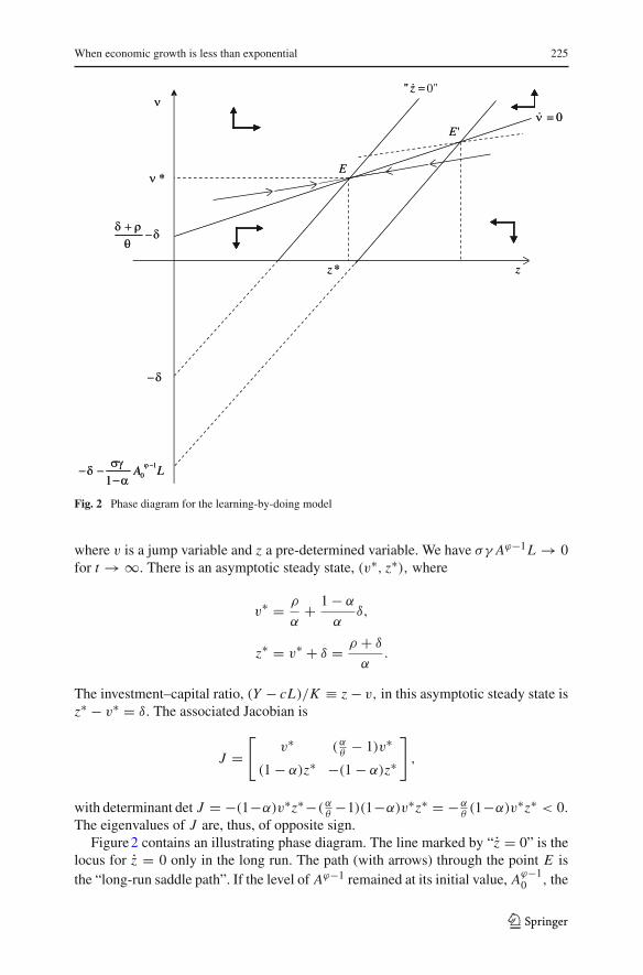
Fig. 2 Phase diagram for the learning-by-doing model
where v is a jump variable and z a pre-determined variable. We have σγ Aϕ−1L → 0for t → ∞. There is an asymptotic steady state, (v∗, z∗), where
v∗ = ρ
α+ 1 − α
αδ,
z∗ = v∗ + δ = ρ + δ
α.
The investment–capital ratio, (Y − cL)/K ≡ z − v, in this asymptotic steady state isz∗ − v∗ = δ. The associated Jacobian is
J =[
v∗ (αθ
− 1)v∗
(1 − α)z∗ −(1 − α)z∗
],
with determinant det J = −(1−α)v∗z∗−(αθ−1)(1−α)v∗z∗ = −α
θ(1−α)v∗z∗ < 0.
The eigenvalues of J are, thus, of opposite sign.Figure 2 contains an illustrating phase diagram. The line marked by “z = 0” is the
locus for z = 0 only in the long run. The path (with arrows) through the point E isthe “long-run saddle path”. If the level of Aϕ−1 remained at its initial value, Aϕ−1
0 , the
123
226 C. Groth et al.
point E ′ would be a steady state and have a saddle path going through it (as illustratedby the dashed line through E ′). But over time, Aϕ−1 decreases and approaches zero.Hence, the point E ′ shifts and approaches the long-run steady state, E .17
The following relations must hold asymptotically:
Y
K= Aσ K α L1−α
K= z∗ so that
K 1−α = Aσ L1−α
z∗ or
K (t) = z∗− 11−α A(t)
σ1−α L =
(α
δ + ρ
) 11−α
L[
A1−ϕ0 + (1 − ϕ)γ Lt
] σ(1−α)(1−ϕ)
=(
α
δ + ρ
) 11−α
L Aσ
1−α
0 (1 + μt)σ
(1−α)(1−ϕ) , where μ ≡ (1 − ϕ)γ Aϕ−10 L > 0.
Thus, in the long run, K features regular growth with positive damping. The dampingcoefficient is (1−α)(1−ϕ)
σ, which may be above or below one, depending on σ. In the
often considered benchmark case, σ = 1−α, the damping coefficient is less than oneif ϕ > 0. Then K features more-than-arithmetic growth. The growth momentum is μ
and is seen to incorporate a scale effect (reflecting the non-rival character of learning).Although K is growing, the growth rate of K tends to zero. The investment–capi-tal ratio, (Y − cL)/K , tends to δ; thus, the saving rate, s ≡ 1 − cL/Y, tends toδK/Y = δ/z∗.
As to manufacturing output, we have in the long run
Y (t) = z∗K (t) =(
α
δ + ρ
) α1−α
L Aσ
1−α
0 (1 + μt)σ
(1−α)(1−ϕ) ,
which is, of course, also regular growth with positive damping. A similar pattern is thentrue for the marginal product of labor w(t) = (1−α)Y (t)/L . The output–capital ratiotends to a constant in the long run. Per capita consumption, c(t) = (1 − s(t))Y (t)/L ,
tends to (1−δ/z∗)Y (t)/L . Finally, the net marginal product of capital, αY (t)/K (t)−δ,
tends to
αz∗ − δ = ρ.
This explains why the growth rate of consumption tends to zero.Although the asymptotic steady state is never reached, the conclusion is that K , Y,
and c in the long run are arbitrarily close to a regular growth pattern with a dampingcoefficient, (1−α)(1−ϕ)
σ, and a growth momentum, μ, the same for all three variables.
In spite of the absence of exponential growth, key ratios such as Y/K and wL/Y tendto be constant in the long run.
17 We shall not here pursue the potentially interesting dynamics going on temporarily, if z0 is above z∗but below the value associated with the point E ′.
123
When economic growth is less than exponential 227
The purpose of this example was to show that a positive rate of time preference,ρ, is no hindrance to such an outcome.18 Given that the regular growth pattern wasinherited from the independent technology path described by (16), this conclusionis perhaps no surprise. In the next section, we consider an example where there ismutual dependence between the development of technology and the remainder of theeconomy.
5 Example 3: investment-specific learning and embodied technical change
Motivated by the steady decline of the relative price of capital equipment and thesecular rise in the ratio of new equipment investment to GNP, Greanwood et al. (1997)developed a tractable model with embodied technical change. The framework hasafterwards been applied and extended in different directions. One such applicationis that of Boucekkine et al. (2003).19 They show that a relative shift from general toinvestment-specific learning externalities may explain the simultaneous occurrence ofa faster decline in the price of capital equipment and a productivity slowdown in the1970s after the first oil price shock.
In this section we present a related model and show that regular, but less-than-expo-nential growth may arise. To begin with, we allow for population growth in order toclarify the role of this aspect for the long-run results. Notation is as above, unlessotherwise indicated. The technology of the economy is described by
Y = K α L1−α, 0 < α < 1, (23)
K = q I − δK , δ > 0, K (0) = K0 given, (24)
q = γ
⎛⎝
t∫
−∞I (τ )dτ
⎞⎠
β
, γ > 0, 0 < β < (1 − α)/α, q(0) = q0 given, (25)
where L = L0ent , n ≥ 0, and K0, q0, and L0 are positive. The new variables areI ≡ Y − cL , i.e., gross investment, and q which denotes the quality (productivity) ofnewly produced investment goods. There is learning by investing, but new learning isincorporated only in newly produced investment goods (this is the embodiment hypoth-esis). Thus, over time each new investment good gives rise to a greater and greateraddition to the capital stock, K , measured in constant efficiency units. The quality q ofinvestment goods of the current vintage is determined by cumulative aggregate grossinvestment as indicated by (25). The parameter β is named the “learning parameter”.The upper bound on β is brought in to avoid explosive growth (infinite output in finitetime). We assume capital goods cannot be converted back into consumption goods.So gross investment, I, is always non-negative.
18 Presupposing δ > 0, qualitatively the same outcome—asymptotic regular growth—emerges for ρ = 0(although in this case we have to use catching-up as optimality criterion).19 We are thankful to Solow for suggesting that embodied technical change might fit our approach and toa referee for suggesting in particular a look at the Boucekkine et al. (2003) paper.
123
228 C. Groth et al.
As we will see, with this technology and the same preferences as in the previousexample, including a positive rate of time preference, the following holds. (a) If n > 0,
the social planner’s solution features exponential growth. (b) If n = 0, the solutionfeatures asymptotic quasi-arithmetic growth; in the limiting case β = (1 − α)/α,
asymptotic exponential growth arises, whereas the case β > (1−α)/α implies explo-sive growth. Before proceeding further, it is worth pointing out two key differencesbetween the present model and that of Boucekkine et al. (2003). In their paper q isdetermined by cumulative net investment. We find it more plausible to have learningassociated with gross investment. And, in fact, this difference turns out to be crucialfor whether n = 0 leads to quasi-arithmetic growth or merely stagnation. Another dif-ference is that in the spirit of our general endeavor, we impose no knife-edge conditionon the learning parameter.20
Since not even the exponential growth case of this model seems explored in theliterature, our exposition will cover that case as well as the less-than-exponentialgrowth case. Many of the basic formulas are common but imply different conclusionsdepending on the value of n.
5.1 The general context
By taking the time derivative on both sides of (25) we get the more convenient differ-ential form
Given ρ > n and initial positive K (0) and q(0), the social planner chooses a plan(c(t))∞t=0, where 0 < c(t) ≤ Y (t)/L(t), so as to maximize
U0 =∞∫
0
c1−θ − 1
1 − θLe−ρt dt
subject to (24), (26), and non-negativity of K for all t. From the first-order conditionsfor an interior solution we find (see Appendix C) that the Keynes–Ramsey rule takesthe form
gc = 1
θ(αz − mδ − ρ), (27)
where z ≡ qY/K (the modified output–capital ratio) and m ≡ pq with p denotingthe shadow price of the capital good in terms of the consumption good. Thus, z is amodified output–capital ratio and m is the shadow price of newly produced investment
20 Differences of minor importance from our perspective include, first, that Boucekkine et al. (2003) letthe embodied learning effect come from accumulated (net) investment per capita (presumably to avoid anykind of scale effect), second, that they combine this effect with a disembodied learning effect.
123
When economic growth is less than exponential 229
goods in terms of the consumption good. Let v ≡ qcL/K (the modified consump-tion–capital ratio), so that, by (24), the growth rate of K is gK = z − v − δ. Further,let h ≡ γ Y/q1/β, so that, by (26), the growth rate of q is gq = (1 − v/z)h; thatis, 1 − v/z is the saving rate, which we will denote s, and h is the highest possiblegrowth rate of the quality of newly produced investment goods. Then, combining thefirst-order conditions and the dynamic constraints (24) and (26) yields the dynamicsystem:
m =[
1 − m
m(δm − αz) +
(1 − v
z
)h
]m, (28)
v =[
1
θ(αz − δm − ρ) − (z − v − δ − n) +
(1 − v
z
)h
]v, (29)
z =[−(1 − α)(z − v − δ − n) +
(1 − v
z
)h
]z, (30)
h =[α(z − v − δ − n) + n − 1
β
(1 − v
z
)h
]h. (31)
Consider a steady state, (m∗, v∗, z∗, h∗), of this system. In steady state, if n > 0,
the economy follows a balanced growth path (BGP for short) with constant growthrates of K , q, Y, and c. Indeed, from (30) and (31) we find the growth rate of K to be
g∗K = z∗ − v∗ − δ = (1 − α)(1 + β)
1 − α(1 + β)n > n iff n > 0. (32)
The inequality is due to the parameter condition
α < 1/(1 + β) (33)
which is equivalent to β < (1−α)/α, the condition assumed in (25). Then, from (30),
g∗q = s∗h∗ =
(1 − v∗
z∗
)h∗ = (1 − α)β
1 − α(1 + β)n = β
1 + βg∗
K . (34)
In view of constancy of h ≡ γ Y/q1/β ,
g∗Y = 1
βg∗
q = 1
1 + βg∗
K . (35)
That is, owing to the embodiment of technical progress Y does not grow as fast as K .
This is in line with the empirical evidence mentioned above. Inserting (27), (32), and(34) into (29) we find
g∗c = 1
θ(αz∗ − m∗δ − ρ) = αβ
1 − α(1 + β)n > 0 iff n > 0. (36)
123
230 C. Groth et al.
This result is, of course, also obtained if we use constancy of v∗/z∗ to conclude thatg∗
c = g∗Y − n. To ensure boundedness of the discounted utility integral we impose the
parameter restriction
(1 − θ)αβ
1 − α(1 + β)n < ρ − n, (37)
which is equivalent to (1 − θ)g∗c < ρ − n.
With these findings we get from (28)
m∗ = α(θg∗c + ρ)
(1 − α + αθ)g∗c + αρ
= θαβn + [1 − α(1 + β)] ρ
(1 − α + αθ)n + [1 − α(1 + β)] ρ≤ 1, (38)
if n ≥ 0, respectively. The parameter restriction (37) implies m∗ > α. Next, from(36),
z∗ = θβ
1 − α(1 + β)n + ρ + δm∗
α> 0, (39)
so that, from (32),
v∗ = θβ − (1 − α)(1 + β)
1 − α(1 + β)n + ρ + δm∗
α− δ, (40)
and
s∗ ≡ 1 − v∗
z∗ = α(1 − α)(1 + β)n + [1 − α(1 + β)] δ
θαβn + [1 − α(1 + β)] (ρ + δm∗)∈ (0, 1). (41)
That s∗ > 0 is immediate from the formula. And s∗ < 1 is implied by v∗ < z∗, whichimmediately follows by comparing (40) and (39). Finally, we have from (34)
h∗ = g∗q
s∗ = (1 − α)βn
[1 − α(1 + β)] s∗ ≥ 0 for n ≥ 0, (42)
respectively.In a BGP the shadow price p (≡m/q) of the capital good in terms of the consump-
tion good is falling since m is constant while q is rising. Indeed,
g∗p = −g∗
q = − (1 − α)β
1 − α(1 + β)n = − β
1 + βg∗
K . (43)
Thus, at the same time as Y/K is falling, the value capital–output ratio Y/(pK ) staysconstant in a BGP. If r denotes the social planner’s marginal net rate of return in terms
123
When economic growth is less than exponential 231
of the consumption good, we have r = [∂Y/∂K − (pδ − p)] /p. Since p ≡ m/q andz ≡ qY/K , we have (∂Y/∂K )/p = αY/(pK ) = αz∗/m∗. Along the BGP, therefore,
r∗ = αz∗
m∗ − (δ − g∗p) = θαβ
1 − α(1 + β)n + ρ = θg∗
c + ρ, (44)
as expected. Since the investment good and the consumption good are produced bythe same technology, we can alternatively calculate r as the marginal net rate of returnto investment: r = (∂Y/∂K − pδ) ∂ K/∂ I = (αY/K − pδ)q. In the BGP we thenget r∗ = αz∗ − m∗δ, which according to (36) amounts to the same as (44).
We have hereby shown that if the learning parameter satisfies (33), a steady stateof the dynamic system is feasible and features exponential semi-endogenous growthif n > 0.21 On the other hand, violation of (33) combined with a positive n implies agrowth potential so enormous that a steady state of the system is infeasible and growthtends to be explosive. But what if n = 0?
5.2 The case with zero population growth
With n = 0 the formulas above are still valid. As a result, the growth rates g∗K , g∗
q , g∗c ,
and g∗p are all zero, whereas m∗ = 1, z∗ = (ρ + δ)/α, v∗ = (ρ + δ)/α − δ, s∗ =
αδ/(ρ +δ) = δ/z∗, and h∗ = 0. By definition we have h ≡ γ Y/q1/β > 0 for all t. Sothe vanishing value of h∗ tells us that the economic system can never attain the steadystate. We will now show, however, that the system converges towards this steady state,which is, therefore, an asymptotic steady state.
When n = 0 and α < 1/(1 + β), we have from purely technological reasonsthat limt→∞ h = 0 (for details, see Appendix C). This implies that for t → ∞ thedynamics of m, v, and z approach the simpler form
m = (1 − m)(δm − αz),
v =[
1
θ(αz − δm − ρ) − (z − v − δ)
]v,
z = −(1 − α)(z − v − δ)z.
The associated Jacobian is
J =⎡⎢⎣
ρ 0 0
− δθv∗ v∗ (α
θ− 1)v∗
0 (1 − α)z∗ −(1 − α)z∗
⎤⎥⎦ .
21 The standard transversality conditions are satisfied at least if θ ≥ 1 (see Appendix C). Owing to non-concavity of the maximized Hamiltonian, however, we have not been able to establish sufficient conditionsfor optimality.
123
232 C. Groth et al.
This is block-triangular and so the eigenvalues are ρ and those of the lower right 2×2sub-matrix of J. Note that this sub-matrix is identical to the Jacobian in the learning-by-doing example of Sect. 4. Accordingly, its eigenvalues are of opposite sign. Sincem and v are jump variables and z is pre-determined, it follows that the asymptoticsteady state is locally saddle-point stable.22
For t → ∞ we, therefore, have s ≡ 1 − v/z → 1 − v∗/z∗ ≡ s∗ and K →L(q/z∗)1/(1−α) (from the definition of z). So, from (26) and (23) it follows that ulti-mately
q = γ qβ−1β s∗K α L1−α = γ Ls∗z∗ −α
1−α q1− 1−α(1+β)(1−α)β ≡ Cq1−ξ , (45)
where C and ξ are implicitly defined constants. This Bernoulli equation has the solu-tion
q(t) = (qξ0 + ξCt)
1ξ = q0(1 + μt)
1ξ , where μ ≡ ξ Lγ δ
(α
ρ + δ
) 11−α
q−ξ0 ,
using the solutions for s∗ and z∗ above. This shows that in the long run the productivityof newly produced investment goods features regular growth with damping coefficientξ = [1 − α(1 + β)] / [(1 − α)β] > 0 and growth momentum μ (which, as expected,is seen to incorporate a scale effect reflecting the non-rival character of learning). Thecorresponding long-run path for capital is
K (t) = L
(q
z∗
) 11−α = L
(α
ρ + δ
) 11−α
q1
1−α
0 (1 + μt)1
(1−α)ξ
and for output
Y (t) = K (t)α L1−α = L
(α
ρ + δ
) α1−α
qα
1−α
0 (1 + μt)α
(1−α)ξ .
The damping coefficient for Y is, thus, (1 − α)ξ/α = [1 − α(1 + β)] /(αβ), sothat more-than-arithmetic growth arises if 1
2 (1 − α)/α < β < (1 − α)/α and less-than-arithmetic growth if β is beneath the lower end of this interval. The same is thentrue for the marginal product of labor, w(t) = (1 − α)Y (t)/L , and for per capitaconsumption, c(t) = (1 − s(t))Y (t)/L , which tends to (1 − δ/z∗)Y (t)/L . For thecapital–output ratio we ultimately have K (t)/Y (t) = q(t)/z∗, which implies more-than-arithmetic growth if β > 1 − α and less-than-arithmetic growth if β < 1 − α.
A new interesting facet compared with the learning-by-doing example of Sect. 4 isthat the shadow price, p, of capital goods remains falling, although at a decreasingrate. This follows from the fact that the shadow price, m ≡ pq, of newly producedinvestment goods in terms of the consumption good tends to a constant at the same
22 The unique converging path unconditionally satisfies the standard transversality conditions (see Appen-dix C).
123
When economic growth is less than exponential 233
time as q is growing, although at a decreasing rate. Finally, the value output–capitalratio Y/(pK ) tends to the constant (qY/K )m = z∗m∗ = z∗ = (ρ + δ)/α and themarginal net rate of return to investment tends to r∗ = αY/(pK ) − δ = ρ.
These results hold when, in addition to n = 0, we have α < 1/(1 + β). In thelimiting case, α = 1/(1 + β), the growth formulas above no longer hold and insteadexponential growth arises. Indeed, the system (28), (29), (30), and (31) is still valid andso is (45) in a steady state of the system. But now ξ = 0. We, therefore, have in a steady
state that q = Cq, which has the solution q(t) = q0eCt , where C ≡ γ Ls∗z∗ −α1−α > 0.
By constancy of h in the steady state, gY = αgK = gq/β = C/β = αC/(1 − α) sothat also Y and K grow exponentially. This is the fully endogenous growth case of themodel. If instead α > 1/(1 + β) we get ξ < 0 in (45), implying explosive growth, anot plausible scenario.
We conclude this section with a remark on why, when exponential growth cannot besustained in a model, sometimes quasi-arithmetic growth results and sometimes com-plete stagnation. In the present context, where we focus on learning, it is the source oflearning that matters. Suppose that, contrary to our assumption above, learning is asso-ciated with net investment, as in Boucekkine et al. (2003). If with respect to the valueof the learning parameter we rule out both the knife-edge case leading to exponentialgrowth and the explosive case, then n = 0 will lead to complete stagnation. Even ifthere is an incentive to maintain the capital stock, this requires no net investment andso learning tends to stop. When learning is associated with gross investment, however,maintaining the capital stock implies sustained learning. In turn, this induces moreinvestment than needed to replace wear and tear and so capital accumulates, althoughat a declining rate. Even if there are diminishing marginal returns to capital, this iscountervailed by the rising productivity of investment goods due to learning. Simi-larly, in the learning-by-doing example of Sect. 4, where learning is simply associatedwith working, learning occurs even if the capital stock is just maintained. Therefore,instead of mere stagnation we get quasi-arithmetic growth.
6 Conclusion
The search for exponential growth paths can be justified by analytical simplicity andthe approximate constancy of the long-run growth rate for more than a century in, forexample, the US. Yet, this paper argues that growth theory needs a more general notionof regularity than that of exponential growth. We suggest that paths along which therate of decline of the growth rate is proportional to the growth rate itself deserve atten-tion; this criterion defines our concept of regular growth. Exponential growth is thelimiting case where the factor of proportionality, the “damping coefficient”, is zero.When the damping coefficient is positive, there is less-than-exponential growth, yetthis growth exhibits a certain regularity and is sustained in the sense that Y/L → ∞for t → ∞. We believe that such a broader perspective on growth will prove particu-larly useful for discussions of the prospects of economic growth in the future, wherepopulation growth (and thereby the expansion of the ultimate source of new ideas) islikely to come to an end.
123
234 C. Groth et al.
The main advantages of the generalized regularity concept are as follows: (1) Theconcept allows researchers to reduce the number of problematic parameter restrictions,which underlie both standard neoclassical and endogenous growth models. (2) Sincethe resulting dynamic process has one more degree of freedom compared to expo-nential growth, it is at least as plausible in empirical terms. (3) The concept covers acontinuum of sustained growth processes which fill the whole range between expo-nential growth and complete stagnation, a range which may deserve more attention inview of the likely future demographic development in the world. (4) As our analysesof zero population growth in the Jones (1995) model, a learning-by-doing model, andan embodied technical change model show, falling growth rates need not mean thateconomic development grinds to a halt. (5) Finally, at least for these three examples,we have demonstrated not only the presence of the generalized regularity pattern, butalso the asymptotic stability of this pattern.
The examples considered are based on a representative agent framework. Our con-jecture is that with heterogeneous agents the generalized notion of regular growthcould be of use as well. Likewise, an elaboration of the embodied technical changeapproach of Sect. 5 might be of empirical interest. For example, Solow (1996) indi-cates that vintage effects tend to be more visible against a background of less-thanexponential growth. As Solow has also suggested,23 there is an array of “behavioral”assumptions waiting for application within growth theory, in particular growth theorywithout the straightjacket of exponential growth.
Appendix A: The canonical Ramsey example
This appendix derives the results reported for Case 4 in Sect. 3. The Hamiltonian forthe optimal control problem is:
H(K , A, c, u, λ1, λ2, t) = c1−θ − 1
1 − θL + λ1(Y − cL) + λ2γ Aϕ(1 − u)L ,
where Y = Aσ K α(uL)1−α and λ1 and λ2 are the co-state variables associatedwith physical capital and knowledge, respectively. Applying the catching-up opti-mality criterion, necessary first-order conditions (see Seierstad and Sydsaeter 1987,pp. 232–234) for an interior solution are:
∂ H
∂c= c−θ L − λ1L = 0, (46)
∂ H
∂u= λ1(1 − α)
Y
u− λ2γ Aϕ L = 0, (47)
∂ H
∂K= λ1α
Y
K= −λ1, (48)
∂ H
∂ A= λ1σ
Y
A+ λ2ϕγ Aϕ−1(1 − u)L = −λ2. (49)
23 Private communication.
123
When economic growth is less than exponential 235
Combining (46) and (48) gives the Keynes–Ramsey rule
gc = 1
θαAσ K α−1(uL)1−α. (50)
Given the definition p = λ2/λ1, (47), (48 ), and (49) yield
gp = αAσ K α−1(uL)1−α − σγ Aϕ−1uL
1 − α− ϕγ Aϕ−1(1 − u)L . (51)
Let x ≡ p A/K . Log-differentiating x w.r.t. time and using (47), (6), (5), and (4) gives(7). Log-differentiating (47) w.r.t. time, using (51), (5), (4) and (6), gives (8). Finally,log-differentiating 1 − s ≡ cL/Y, using (50), (4), (6) and (5), gives (9).
In the text we defined μ ≡ (1 − ϕ)γ (1 − u∗)L A0ϕ−1.
Lemma 1 In a steady state of the system (7), (8), and (9)
λ1(t)K (t) = λ1(0)K0(1 + μt)ω, and (52)
λ2(t)A(t) = λ2(0)A0(1 + μt)ω, (53)
where
ω ≡ σ + 1 − ϕ − θ [σ + α(1 − ϕ)]
(1 − α)(1 − ϕ).
Proof As shown in the text, in a steady state of the system we have Y (t)/K (t) =(Y (0)/K0)(1 + μt)−1 so that
t∫
0
Y (τ )
K (τ )dτ = Y (0)
K0μ−1 ln(1 + μt) = θ [σ + α(1 − ϕ)]
α(1 − α)(1 − ϕ)ln(1 + μt),
where the latter equality follows from (13), (11), (10), and the definition of μ. There-fore, by (48) and (13),
λ1(t)K (t) = λ1(0)e−α∫ t
0Y (τ )K (τ )
dτ K0(1 + μt)σ+1−ϕ
(1−α)(1−ϕ)
= λ1(0)K0(1 + μt)σ+1−ϕ
(1−α)(1−ϕ)− θ[σ+α(1−ϕ)]
(1−α)(1−ϕ) ,
which proves (52).From (49) and p ≡ λ2/λ1 follows that in steady state
λ2
λ2= −σY
p A− ϕγ Aϕ−1(1 − u∗)L = −γ
(σu∗
1 − α+ ϕ(1 − u∗)
)L Aϕ−1
0 (1 + μt)−1,
123
236 C. Groth et al.
where the latter equality follows from (4), (12), and (11). Hence,
t∫
0
λ2(τ )
λ2(τ )dτ = −ϕ − σ − α + θ [σ + α(1 − ϕ)]
(1 − α)(1 − ϕ)ln(1 + μt),
by (10) and the definition of μ. Therefore,
λ2(t)A(t) = λ2(0)e∫ t
0λ2(τ )
λ2(τ )dτ
A0(1 + μt)1
1−ϕ
= λ2(0)A0(1 + μt)1
1−ϕ− ϕ−σ−α+θ[σ+α(1−ϕ)]
(1−α)(1−ϕ) ,
which proves (53). � We have ω < 0 if and only if
θ > (σ + 1 − ϕ)/ [σ + α(1 − ϕ)] . (54)
Hence, by Lemma 1 follows that the “standard” transversality conditions,limt→∞ λ1(t)K (t) = 0 and limt→∞ λ2(t)A(t) = 0, hold along the unique regu-lar growth path if and only if (54) is satisfied. This condition is a little stronger thanθ > 1. Our conjecture is that these transversality conditions together with the first-order conditions are necessary and sufficient for an optimal solution. This guessednecessity and sufficiency is based on the saddle-point stability of the steady state (seebelow). Yet, we have so far no proof. The maximized Hamiltonian is not jointly con-cave in (K , A) unless σ = ϕ(1 − α). Thus, the Arrow sufficiency theorem does notapply; hence, neither does the Mangasarian sufficiency theorem (see Seierstad andSydsaeter 1987). So, we only have a conjecture. (This is of course not a satisfactorysituation, but we might add that this situation is quite common in the semi-endogenousgrowth literature, although authors are often silent about the issue.)
As to the stability question it is convenient to transform the dynamic system. Wedo that in two steps. First, let z ≡ xu and q ≡ (1 − s)xu. Then the system (7), (8),and (9) becomes
z = γ L Aϕ−1(
1 − ϕ + σ
α− z − (1 − ϕ)u
)z,
u = γ L Aϕ−1(
σ
α+ σ
1 − αu − q
1 − α
)u,
q = γ L Aϕ−1(
1 − ϕ + α − θ
(1 − α)θz − (1 − ϕ)u + 1
1 − αq
)q.
The steady state of this system is (z∗, u∗, q∗) = (x∗u∗, u∗, (1 − s∗)x∗u∗). Sec-ond, this system can be converted into an autonomous system in “transformed time”τ = ln A(t) ≡ f (t). With u(t) < 1, f ′(t) = γ A(t)ϕ−1(1 − u(t))L > 0 and we
123
When economic growth is less than exponential 237
have t = f −1(τ ). Thus, considering z(τ ) ≡ z( f −1(τ )), u(τ ) ≡ u( f −1(τ )) andq(τ ) ≡ q( f −1(τ )), the above system is converted into
dz
dτ=
(1 − ϕ + σ
α− z − (1 − ϕ)u
) z
1 − u,
du
dτ=
(σ
α+ σ
1 − αu − q
1 − α
)u
1 − u,
dq
dτ=
(1 − ϕ + α − θ
(1 − α)θz − (1 − ϕ)u + 1
1 − αq
)q
1 − u.
The Jacobian of this system, evaluated in steady state, is
J =⎡⎢⎣
−z∗ −(1 − ϕ)z∗ 0
0 σ1−α
u∗ − 11−α
u∗α−θ
(1−α)θq∗ −(1 − ϕ)q∗ 1
1−αq∗
⎤⎥⎦ · 1
1 − u∗ .
The determinant is
det J = −σθ + (θ − 1)(1 − ϕ)α
(1 − α)2θz∗u∗q∗ < 0,
in view of θ > 1. The trace is
trJ = (α − s∗)x∗ + σ
1 − α
u∗
1 − u∗ = [σ + α(1 − ϕ)] (2θ − 1) − σ − 1 + ϕ
(1 − α)(θ − 1) [σ + α(1 − ϕ)]
σu∗
1 − u∗ >0,
in view of the transversality condition (54). Thus, J has one negative eigenvalue, η1,
and two eigenvalues with positive real part. All three variables, z, u and q, are jumpvariables, but z and u are linked through
z = 1 − α
γ LαAσ+1−ϕ
(u
K
)1−α
≡h(u, A, K ). (55)
In order to check existence and uniqueness of a convergent solution, letx = (x1, x2, x3) ≡ (z, u, q) and x = (x1, x2, x3) ≡ (z∗, u∗, q∗). Then, in a smallneighborhood of x any convergent solution is of the form x(τ ) = Cveη1τ + x, whereC is a constant, depending on initial A and K , and v = (v1, v2, v3) is an eigenvectorassociated with η1 so that
(−z∗ − η1)v1 − (1 − ϕ)z∗v2 = 0, (56a)
0 +(
σ
1 − αu∗ − η1
)v2 − 1
1 − αu∗v3 = 0, (56b)
α − θ
(1 − α)θq∗v1 − (1 − ϕ)q∗v2 +
(1
1 − αq∗ − η1
)v3 = 0. (56c)
123
238 C. Groth et al.
We see that vi = 0, i = 1, 2, 3. Initial transformed time is τ0 = ln A0 and wehave x(τ0) = (h(u(0), A0, K0), u(0), q(0)) for A(0) = A0, and K (0) = K0 (bothpre-determined), where we have used (55) for t = 0. Hence, coordinate-wise,
x1(τ0) = Cv1eη1τ0 + z∗ = h(u(0), A0, K0), (57)
x2(τ0) = Cv2eη1τ0 + u∗ = u(0), (58)
x3(τ0) = Cv3eη1τ0 + q∗ = q(0). (59)
This system has a unique solution in (C, u(0), q(0)); indeed, substituting (58) and(59) into (57), setting v1 = 1 and using z∗ = x∗u∗, gives
1
v2u(0) + u∗(x∗ − 1
v2) = h(u(0), A0, K0). (60)
It follows from Lemma 2 that, given θ > 1, (60) has a unique solution in u(0). Withthe pre-determined initial value of the ratio, Aσ+1−ϕ/K 1−α, in a small neighborhoodof its steady state value (which is γ Lαx∗u∗α/(1 − α)), the solution for u(0) is closeto u∗; hence it belongs to the open interval (0, 1).
Lemma 2 Assume θ > 1. Then 1/v2 > x∗.
Proof From (56a),
v2 = −z∗ − η1
(1 − ϕ)z∗ . (61)
Substituting v1 = 1 together with (56b) into (56c) gives
α − θ
(1 − α)θq∗ − (1 − ϕ)q∗v2 +
(1
1 − αq∗ − η1
) (σ − (1 − α)η1
u∗
)v2 ≡ Q(v2, η1) = 0.
Replacing η1 and v2 in (61) by η and w(η), respectively, we see that P(η) ≡Q(w(η), η) is the characteristic polynomial of degree 3 corresponding to J . Now,
P(−z∗) = α − θ
(1 − α)θq∗ < 0,
as θ > 1. Consider η0 ≡ −(1 − ϕ)z∗/x∗ − z∗ < −z∗. Clearly, w(η0) = 1/x∗. IfP(η0) > 0, then the unique negative eigenvalue η1 satisfies η0 < η1 < −z∗, implyingthat v2 ≡ w(η1) < 1/x∗, in view of w′(η) < 0; hence 1/v2 > x∗. It remains to provethat P(η0) > 0. We have
123
When economic growth is less than exponential 239
P(η0) = α−θ
(1 − α)θq∗−(1 − ϕ)q∗w(η0)+
(1
1 − αq∗−η1
) (σ − (1 − α)η1
u∗
)w(η0)
= α − θ
(1 − α)θq∗ − (1 − ϕ)q∗
x∗ +(
1
1 − αq∗ − η0
) (σ − (1 − α)η0
u∗
)1
x∗
= α(1 − θ) [(1 − α)(1 − ϕ) + σ ] (1 − s∗)x∗u∗
(1 − α)θσ
+ [(1 − α)(1 − ϕ) + σ ] (1 − s∗) + (1 − α)σ
1 − αu∗ + 1 − ϕ
x∗ σu∗ + 1 − α
u∗x∗ η20
= θ − 1
θ[σ + α(1 − ϕ)] + 1 − α
u∗x∗ η20 > 0,
where the third equality is based on reordering and the definition of q∗, whereas thelast equality is based on the formulas for x∗, u∗, and s∗ in (10); finally, the inequalityis due to θ > 1. �
Appendix B: The learning-by-doing example
By (19), the transversality condition (21) can be written
limt→∞ c(t)−θe−ρt K (t) = 0,
which is obviously satisfied along the asymptotic regular growth path, since ρ > 0,
and c and K feature less than exponential growth. In the text we claimed that the first-order conditions together with the transversality condition are sufficient for an optimalsolution. Indeed, this follows from the Mangasarian sufficiency theorem, since H isjointly concave in (K , c) and the state and co-state variables are non-negative for allt ≥ 0, cf. Seierstad and Sydsaeter (1987, pp. 234–235). Uniqueness of the solutionfollows because H is strictly concave in (K , c) for all t ≥ 0.
Appendix C: The investment-specific learning example
The current-value Hamiltonian for the optimal control problem is:
H(K , q, c, λ1, λ2, t) = c1−θ − 1
1 − θL + λ1 [q(Y − cL) − δK ] + λ2γ q
β−1β (Y − cL),
where Y = K α L1−α and λ1 and λ2 are the co-state variables associated with physicalcapital and the quality of newly produced investment goods, respectively. An interior
123
240 C. Groth et al.
solution will satisfy the first-order conditions
∂ H
∂c= c−θ L − λ1q L − λ2γ q
β−1β L = 0, (62)
∂ H
∂K= λ1(qα
Y
K− δ) + λ2γ q
β−1β α
Y
K= ρλ1 − λ1, (63)
∂ H
∂q= λ1(Y − cL) + λ2γ
β − 1
βq
−1β (Y − cL) = ρλ2 − λ2. (64)
The first-order conditions imply
Lemma 3 ddt
(c−θ ) = c−θ (ρ − αq YK ) + λ1qδ.
Proof Let
u ≡ c−θ − λ1q = λ2γ qβ−1β = λ2
q
I, (65)
by (62) and (26), respectively. Then, using (64) and I ≡ Y − cL ,
gu = gλ2 + β − 1
βgq = ρ −
(λ1
λ2+ γ
β − 1
βq
−1β
)I + β − 1
βγ q
−1β I = ρ − λ1
λ2I,
(66)
so that
u = ρu − λ1
λ2I u = ρu − λ1q, (67)
by (65). Rewriting (65) as c−θ = λ1q + u, we find
d
dt(c−θ ) = λ1q+λ1q + u =ρu+λ1q =ρc−θ −(ρλ1 − λ1)q (from (67) and (65))
= ρc−θ −[(λ1q + λ2γ q
β−1β )α
Y
K− λ1δ
]q = ρc−θ − c−θαq
Y
K+ λ1qδ,
where the two latter equalities come from (63) and (62), respectively. � From Lemma 3 follows
gc = −1
θ
ddt
(c−θ )
c−θ= 1
θ(αz − mδ − ρ) ,
using that z ≡ qY/K and
m ≡ pq ≡ (λ1/c−θ )q = λ1
λ1q + λ2γ qβ−1β
q, (68)
by (62). This proves (27).
123
When economic growth is less than exponential 241
The conjectured necessary and sufficient transversality conditions are limt→∞λ1(t)e−ρt K (t) = 0 and limt→∞ λ2(t)e−ρt q(t) = 0. We now check whether theseconditions hold in the steady state. First, note that (63) and (65) give
gλ1 = ρ + δ − c−θ
λ1α
Y
K= ρ + δ − α
Y
pK= ρ + 1
m(mδ − αz)
= ρ − 1
m∗ (θg∗c + ρ) = (1 − α + αθ)g∗
c
α
in steady state, by (38). Further, we have in steady state g∗K = g∗
c /α + n. Hence,g∗λ1
+ g∗K − ρ = (1 − θ)g∗
c + n − ρ < 0, by the parameter restriction (37). Thus thefirst transversality condition holds for all θ > 0.
From (66)
gλ2 +gq − ρ = ρ − λ1
λ2I − β − 1
βgq + gq − ρ = − m
1 − mγ q
−1β I + 1
βgq (by (68))
= − m
1 − mgq + 1
βgq =−(θg∗
c +ρ)+ 1 − α
αβg∗
c = 1 − α(1 + θβ)
1 − α(1 + β)n−ρ,
in steady state, by (38), (34), and (36). It follows that θ ≥ 1 is sufficient for the secondtransversality condition to hold. If n = 0, no particular condition on θ is needed toensure this transversality condition.
It remains to show:
Lemma 4 If n = 0 and α < 1/(1 + β), then for purely technological reasonslimt→∞ h = 0.
Proof Let n = 0 and α < 1/(1 + β). We have h ≡ Y/q1/β = K α L1−α/q1/β, whereL is constant and q is always non-decreasing, by (26). There are two cases to consider.Case 1: q � ∞ for t → ∞. Then, by (25), for t → ∞, I → 0, hence K → −δK ,
and so K → 0, whereby h → 0. Case 2: q → ∞ for t → ∞. If K � ∞ for t → ∞,
we are finished. Suppose K → ∞ for t → ∞. Then, for t → ∞ we must havegK = sz − δ ≥ 0 so that z � 0, in view of δ > 0. In addition, defining x ≡ zhβ, weget x = K α(1+β)−1L(1−α)(1+β) → 0 for t → ∞. It follows that h ≡ (x/z)1/β → 0for t → ∞, since α < 1/(1 + β). �
References
Aghion, P., Howitt, P.: A model of growth through creative destruction. Econometrica 60, 323–351 (1992)Alvarez-Pelaez, M.J., Groth, C.: Too little or too much R&D? Eur Econ Rev 49, 437–456 (2005)Arnold, L.: The dynamics of the Jones R&D growth model. Rev Econ Dyn 9, 143–152 (2006)Arrow, K.J.: The economic implications of learning by doing. Rev Econ Stud 29, 153–173 (1962)Asheim, G.B., Buchholz, W., Hartwick, J.M., Mitra, T., Withagen, C.A.: Constant savings rates and quasi-
arithmetic population growth under exhaustible resource constraints. J Environ Econ Manag 53, 213–229 (2007)
Attanasio, O., Weber, G.: Is Consumption Growth Consistent with Intertemporal Optimization? J PoliticalEcon 103, 1121–1157 (1995)
Blanchard, O.J., Fischer, S.: Lectures on Macroeconomics. Cambridge: MIT Press (1989)Boucekkine, R., del Rio, F., Licandro, O.: Embodied technological change, learning-by-doing and the
productivity slowdown. Scand J Econ 105(1), 87–97 (2003)Dasgupta, P., Heal, G.: Economic Theory and Exhaustible Resources. Cambridge: Cambridge University
change. Am Econ Rev 87(3), 342–362 (1997)Grossman, G.M., Helpman, E.: Innovation and Growth in the Global Economy. Cambridge: MIT
Press (1991)Growiec, J.: Beyond the linearity critique: the knife-edge assumption of steady-state growth. Econ
Theory 31(3), 489–499 (2007)Growiec, J.: Knife-edge conditions in the modeling of long-run growth regularities. Working Paper, Warsaw
School of Economics (2008)Hakenes, H., Irmen, A.: On the long-run evolution of technological knowledge. Econ Theory 30, 171–
180 (2007)Hartwick, J.M.: Intergenerational equity and the investing of rents from exhaustible resources. Am Econ
Rev 67, 972–974 (1977)Jones, C.I.: R&D-based models of economic growth. J Political Econ 103, 759–784 (1995)Jones, C.I.: Growth and ideas. In: Aghion, P., Durlauf, S.N. (eds.) Handbook of Economic Growth,
vol. I.B., pp. 1063–1111. Amsterdam: Elsevier (2005)Kremer, M.: Population growth and technological change: one million B.C. to 1990. Q J Econ 108, 681–
716 (1993)McCallum, B.T.: Neoclassical vs. endogenous growth analysis: an overview. Federal Reserve
Bank Richmond Econ Q Rev 82(Fall), 41–71 (1996)Mitra, T.: Limits on population growth under exhaustible resource constraints. Int Econ Rev 24, 155–
168 (1983)Pezzey, J.: Exact measures of income in a hyperbolic economy. Envir Dev Econ 9, 473–484 (2004)Ramsey, F.P.: A mathematical theory of saving. Econ J 38, 543–559 (1928)Romer, P.M.: Endogenous technological change. J Political Econ 98, 71–101 (1990)Seierstad, A., Sydsaeter, K.: Optimal Control Theory with Economic Applications. Amsterdam: North
Holland (1987)Solow, R.M.: Intergenerational equity and exhaustible resources. Rev Econ Stud (Symposium Issue),
29–45 (1974)Solow, R.M.: Perspectives on growth theory. J Econ Perspect 8, 45–54 (1994)Solow, R.M.: Growth Theory without “Growth” —Notes Inspired by Rereading Oelgaard. Nationaloeko-
nomisk Tidsskrift—Festskrift til Anders Oelgaard, 87–93 (1996)Solow, R.M.: Growth Theory. An Exposition. Oxford: Oxford University Press (2000)United Nations: World Population Prospects. The 2004 Revision. New York (2005)Young, A.: Growth without scale effects. J Political Econ 106, 41–63 (1998)