101
Whole-system cost of variable renewables in future GB electricity system Joint industry project with RWE Innogy, Renewable Energy Systems and ScottishPower Renewables October 2016
| Date post: | 09-Sep-2018 |
| Category: |
Documents |
| Upload: | trinhhuong |
| View: | 215 times |
| Download: | 0 times |
Whole-system cost of variable renewables in
future GB electricity system
Joint industry project with
RWE Innogy, Renewable Energy Systems and
ScottishPower Renewables
October 2016
Imperial College Project Team:
Prof. Goran Strbac
Dr. Marko Aunedi
Acknowledgments
The authors would like to thank all experts from the project Sponsors’ group who have pro-
vided very valuable input and feedback over the course of the project: Alex Murley (RWE
Innogy), Alex Coulton (Renewable Energy Systems), Fiona Shepherd and Christopher
McGinnis (both from ScottishPower Renewables).
The authors would also like to express their gratitude to the Engineering and Physical Sci-
ences Research Council for the support obtained through the Whole Systems Energy Model-
ling Consortium and Energy Storage for Low Carbon Grids grants. These programmes en-
abled the fundamental research that led to the development of the modelling framework for
quantifying whole-system costs used in this study.

Contents
Executive Summary 1
1. Introduction 14
1.1. Background 14
1.2. Concept of system integration costs of generation technologies 14
1.3. Challenges of integrating low-carbon generation 15
1.4. Key objective 16
2. Methodology for quantifying whole-system costs of low-carbon technologies 17
2.1. Whole-system assessment of electricity systems 17
2.2. Valuation of flexible options in future systems 18
2.3. Method for calculating SIC 18
3. Scenarios and assumptions 20
3.1. Description of scenarios 20
3.2. Assumptions on generation technologies 21
3.2.1. Generation capacity 21
3.2.2. Capacity factors 22
3.2.3. Geographical distribution of generation capacity 24
3.2.4. Cost assumptions 25
3.3. Demand assumptions 25
3.4. Flexibility assumptions 26
3.4.1. Deployment of flexible options 26
3.4.2. Improved system operation in Modernisation scenario 27
3.5. Other assumptions 28
3.5.1. Carbon intensity target 28
3.5.2. Fuel and carbon prices 28
3.5.3. System security assumptions 29
3.5.4. Interaction with neighbouring systems 29
3.6. Optimisation set-up for scenarios and SIC studies 30
3.6.1. Counterfactual scenarios 30
3.6.2. System Integration Cost studies 31
4. System Integration Costs of low-carbon technologies 33
4.1. Counterfactual scenarios 33
4.1.1. Optimised generation portfolios 33
4.1.2. Annual energy production and utilisation factors 35
4.1.3. Total system cost comparison across 2030 scenarios 38
4.2. Technology-specific integration costs 42
4.2.1. Offshore wind 42
4.2.2. Onshore wind 45
4.2.3. Solar PV 47

4.2.4. Biomass 49
5. Illustration of key aspects of hourly system operation 52
5.1. Impact of flexible options on residual demand 52
5.2. Winter vs. summer system operation 56
6. Sensitivity analysis 58
6.1. Impact of retiring biomass before 2030 58
6.2. Impact of more ambitious carbon target in 2030 60
6.3. Impact of system flexibility 63
6.4. Impact of largest generator size and relaxed minimum CCGT capacity 67
7. Modernised system operation 71
7.1. Challenges of integrating variable renewables 71
7.2. Market value of energy and ancillary services in future systems 74
7.3. Enhancing market and regulatory framework to facilitate deployment of energy storage and DSR 74
7.4. Opportunities and barriers for gas plant of enhanced flexibility 75
7.5. Enhancing EU market design to facilitate cross-border energy, capacity and reserve trading 79
8. Conclusions 81
Appendix A. Overview of the methodology for whole-system analysis of electricity systems 84
A.1. Whole-systems modelling of electricity sector 84
A.2. WeSIM problem formulation 86
A.3. System topology 91
A.4. Distribution network investment modelling 92
A.5. Demand modelling 95

1
Executive Summary
Background
With nearly half of UK’s generation capacity expected to retire in the build up to 2030, the
UK’s electricity system is facing exceptional challenges in the coming decades. Replacing
this generation capacity will for the most part need to be achieved with low-carbon electricity
generation technologies if we are to meet our carbon emission reduction targets and this will
need to be done whilst maintaining security of supply. The UK’s electricity sector is in par-
ticular expected to deliver significant reductions in its carbon emissions by 2030, which will
require increasing deployment of low-carbon generation technologies such as renewables,
nuclear, biomass, carbon capture and storage, etc. In the context of the Contracts for Differ-
ence (CfD) mechanism, which allocates payments to low-carbon generators, there is a ques-
tion over whether selecting technologies solely based on their levelised cost would deliver
decarbonisation at the lowest overall cost. Generally, variable renewable generation tech-
nologies would impose certain types of costs on the wider system, for example through the
need for more back-up capacity and balancing services (although all generation options may
imply some system costs).
There are two key factors which may reduce the ability of the system to accommodate the
combination of inflexible low-carbon generation and variable renewables:
Increase in system balancing requirements: Reserve requirements will increase due to
higher generation output fluctuations and consequently higher forecasting errors asso-
ciated with high RES penetrations. At the same time, given that wind and solar PV
represent non-synchronous power sources that tend not to contribute to system inertia1,
the overall system inertia will decrease during periods of high variable renewable out-
put. When combined with an increased size of largest generator loss in line with the
expected capacities of future nuclear generators, this will lead to higher requirements
for primary frequency regulation. The importance of frequency regulation in the fu-
ture GB system is hence expected to increase dramatically.
Limited flexibility of present system: At present, flexibility is provided by conven-
tional gas and coal generators, which are typically characterised by a limited amount
of frequency control they can provide and a relatively high minimum stable genera-
tion. Both of these features may represent limiting factors for the amount of renew-
able generation that can be accommodated in the system. Conventional generation
technologies with significantly enhanced flexibility are already available, but the lack
of appropriate market signals has so far suppressed their deployment. In this context,
energy storage technologies and demand-side response could also significantly en-
hance system flexibility.
1 It is noted that onshore and offshore wind turbines have the technical capability to provide “synthetic inertia” through
the adoption of advanced control schemes that enable the release of their kinetic energy into the grid during a contin-
gency. Nevertheless, current regulatory framework does not require wind generators to provide inertial response to the
system.
2
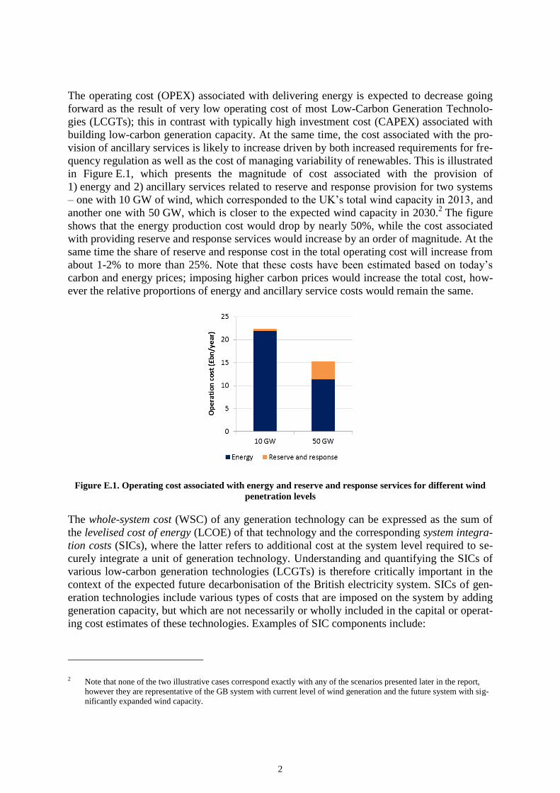
The operating cost (OPEX) associated with delivering energy is expected to decrease going
forward as the result of very low operating cost of most Low-Carbon Generation Technolo-
gies (LCGTs); this in contrast with typically high investment cost (CAPEX) associated with
building low-carbon generation capacity. At the same time, the cost associated with the pro-
vision of ancillary services is likely to increase driven by both increased requirements for fre-
quency regulation as well as the cost of managing variability of renewables. This is illustrated
in Figure E.1, which presents the magnitude of cost associated with the provision of
1) energy and 2) ancillary services related to reserve and response provision for two systems
– one with 10 GW of wind, which corresponded to the UK’s total wind capacity in 2013, and
another one with 50 GW, which is closer to the expected wind capacity in 2030.2 The figure
shows that the energy production cost would drop by nearly 50%, while the cost associated
with providing reserve and response services would increase by an order of magnitude. At the
same time the share of reserve and response cost in the total operating cost will increase from
about 1-2% to more than 25%. Note that these costs have been estimated based on today’s
carbon and energy prices; imposing higher carbon prices would increase the total cost, how-
ever the relative proportions of energy and ancillary service costs would remain the same.
Figure E.1. Operating cost associated with energy and reserve and response services for different wind
penetration levels
The whole-system cost (WSC) of any generation technology can be expressed as the sum of
the levelised cost of energy (LCOE) of that technology and the corresponding system integra-
tion costs (SICs), where the latter refers to additional cost at the system level required to se-
curely integrate a unit of generation technology. Understanding and quantifying the SICs of
various low-carbon generation technologies (LCGTs) is therefore critically important in the
context of the expected future decarbonisation of the British electricity system. SICs of gen-
eration technologies include various types of costs that are imposed on the system by adding
generation capacity, but which are not necessarily or wholly included in the capital or operat-
ing cost estimates of these technologies. Examples of SIC components include:
2 Note that none of the two illustrative cases correspond exactly with any of the scenarios presented later in the report,
however they are representative of the GB system with current level of wind generation and the future system with sig-
nificantly expanded wind capacity.

3
Increased balancing cost associated with: a) increased requirements for system re-
serve due to higher uncertainty of variable renewable generation output, and
b) increased requirements for fast frequency regulation (response) due to reduced sys-
tem inertia as well as larger maximum generating unit size.
Network reinforcements required in interconnection, transmission and distribution in-
frastructure (e.g. transmission reinforcement to connect remote wind resources).
Increased backup capacity cost due to limited ability of e.g. variable renewable tech-
nologies to displace “firm” generation capacity needed to ensure adequacy of supply.
Cost of maintaining system carbon emissions, as the addition of certain technologies
may cause the overall emission performance of the system to deteriorate, requiring
that additional low-carbon capacity is installed to maintain the same level of carbon
emissions.
Some of these components, such as increased balancing or network cost are already reflected
to some extent in current charges imposed on generators, such as the balancing payments
(BSUoS), or transmission and distribution charges (TNUoS and DUoS). Nevertheless, these
charges are not fully cost-reflective3. Some of the above components such as the backup ca-
pacity are not currently included in LCOE assessments in any form whilst other components
such as constraint payments are completely imposed on distributed generators through the
bilateral conditional grid connection agreements which include provision for uncompensated
constraint.
Understanding the WSC of technology requires the quantification of SICs in addition to the
cost of building and operating low-carbon generation capacity, i.e. their Levelised Cost of
Electricity (LCOE). SIC therefore represents a critical input into planning for a cost-effective
transition towards a low-carbon electricity system, enabling the development of policies and
procurement mechanisms that consider both private and wider system costs of different tech-
nologies. This study seeks to quantify and examine in detail the SIC of low-carbon generation
technologies such as nuclear, biomass, variable renewable generation technologies, with par-
ticular focus on onshore and offshore wind, in the context of the future, largely decarbonised
UK electricity system. The report also focusses on quantifying the total system cost of the
future UK system where the emphasis is expected to shift towards low-carbon technologies
with generally high investment cost but low operating cost.
This report, however, does not consider existing market arrangements or dynamics. It does
not for instance account for the part of SIC that might already be paid for by generators
through market arrangements such as BSUoS charges or Grid connection agreements or as
part of discounts embedded with Power Purchase Agreements to reflect imbalance risk.
3 For a more detailed discussion on the issue, see a recent study prepared by NERA Economic Consulting and Imperial
College London for the Committee on Climate Change: “System integration costs for alternative low carbon generation
technologies – policy implications”, available here: https://www.theccc.org.uk/publication/system-integration-costs-for-
alternative-low-carbon-generation-technologies-policy-implications/.

4
Methodology
This report quantifies the relative integration cost reflecting the difference between the sys-
tem externalities of pairs of LCGTs, with nuclear power chosen to represent the benchmark
LCGT against which the relative SIC of other LCGTs (wind, solar and biomass) are quanti-
fied. The choice of nuclear as the benchmark technology is somewhat arbitrary but is moti-
vated by nuclear being a baseload LCGT and enables other LCGTs to be compared against
the same reference technology. The interpretation of relative SIC compared against nuclear
generators should be that if the SIC for a given LCGT is higher than its corresponding LCOE
cost advantage against nuclear, this suggests that a unit of this technology has a higher whole-
system cost i.e. provides a lower net marginal benefit to the system than a unit of nuclear ca-
pacity (and vice versa).
Different components of SIC are incurred in different segments of the electricity system, such
as generation, transmission or distribution infrastructure, or are a part of system operation and
balancing cost. Therefore, the quantitative framework applied to evaluate the SIC is based on
the whole-system modelling approach (WeSIM model), with the ability to simultaneously
make investment and operation decisions with hourly time resolution, while capturing the
interactions between different time scales as well as across different asset types in the elec-
tricity system. At the same time the model can also consider a broad range of flexible tech-
nologies such as energy storage or demand-side response (DSR). In this study the WeSIM
model was applied to the interconnected GB electricity system while also considering two
neighbouring systems: Ireland and Continental Europe (CE). Important feature of the model
is in the ability to impose carbon emission target while ensuring that the security of supply
standards are met.
Instead of focusing on quantifying the components of SIC separately (e.g. only the additional
balancing or additional network cost), this study quantifies the whole-system impact of add-
ing a unit of LCGT into an electricity system while maintaining a given carbon intensity tar-
get. The method adopted to quantify the SIC assumes nuclear power as the benchmark LCGT,
and is based on optimised replacement, assuming that 1 GW of nuclear capacity is removed
from the system, while the model is allowed to optimally increase the capacity of another
LCGT (e.g. wind or solar) while at the same time maintaining the same overall GB system
emissions. No change in the capacities of other LCGTs is allowed in this method; the model
is only allowed to adjust conventional capacity if cost-efficient. Similarly, the volumes of en-
ergy storage, DSR and interconnection in SIC studies (i.e. when optimising the system where
1 GW of nuclear is replaced by another LCGT) are also kept constant at the counterfactual
scenario level.4
Changes in total system cost, excluding the investment and operation cost (i.e. LCOE) of the
pairs of technologies involved in the substitution (e.g. removed nuclear and added wind ca-
pacity), are divided by the annual output of the added low-carbon technology to establish its
relative SIC against nuclear power in £/MWh. Also, in this method any cost of LCGT capac-
4 If the volumes of flexible options are allowed to be cost-optimally adjusted in SIC studies together with conventional
generation capacities, this could result in a lower observed change in total system cost. In that context the integration
cost results in this study represent conservative estimates of SIC of LCGTs.

5
ity added in excess of the energy-equivalent5 volume is factored into the total cost differential
between the original system and a given SIC study. This also means that any cost associated
with curtailing LCGT output during periods of oversupply is included in the SIC.
Scenarios and assumptions
Power system scenarios cover the period between 2015 and 2030, with a single scenario cov-
ering years 2015, 2020 and 2025, and a range of seven 2030 scenarios with varying level of
system flexibility or alternative low-carbon generation mixes. A number of sensitivity studies
have also been done in addition to the core scenarios. All scenarios assume a significant ex-
pansion of low-carbon generation capacity (primarily nuclear, wind and PV). The scenarios
assumed a certain level of targeted carbon intensity for the electricity system; in the basic set
of studies this target was set at 100 g/kWh in 2030, although sensitivity studies have been run
with the 50 g/kWh target as well (which could be used as an indication of system circum-
stances around year 2035).
The following core scenarios were considered in 2030:
1. Mid Flexibility (“Mid Flex”): Central scenario with high wind deployment, reaching
up to 31 GW of offshore and 20 GW of onshore wind in 2030. This scenario has
moderate levels of nuclear (8.2 GW), assuming the addition of 4.5 GW of new capac-
ity by 2030, and 20 GW of PV capacity. It also has a moderately high deployment
level of flexible options: 10 GW of new distributed storage, 50% of DSR uptake and
11.3 GW of interconnection capacity.
2. Low flexibility (“Low Flex”): Same as Mid Flex, but with less ambitious deployment
of flexible options: 5 GW of new storage, 25% DSR uptake and 10 GW of intercon-
nection.
3. Modernisation: Same as Mid Flex, but with a range of measures to improve system
operation (concerning wind predictability, capability to provide ancillary services
etc.).
4. High flexibility (“Mega Flex”): Scenario with similar generation mix as the Mid Flex,
but with enhanced flexibility i.e. higher storage (15 GW) and interconnection capacity
(15 GW) and greater DSR uptake than the Mid Flex (100%).
5. Onshore Capped: Scenario with no new onshore wind deployment beyond today’s
level (dropping to around 8 GW by 2030 due to decommissioning), but compensated
by a more intensive expansion of offshore wind until 2030. Nuclear and PV capacity
are at the Mid Flex level.
6. Nuclear Centric: This represents a theoretical alternative technological solution to a
high variable LCGT mix for achieving the UK’s decarbonisation agenda. Whilst a
5 Energy equivalence here means that the removed and added capacities are capable of providing the same nominal an-
nual output (e.g. if the annual utilisation of nuclear is 90% and that of offshore wind is 43%, then it would take about
2.1 GW of wind capacity to produce the same output as 1 GW of nuclear).

6
more ambitious nuclear expansion in this scenario (16.4 GW in 2030) seems un-
achievable to deliver from today’s perspective, this scenario nevertheless offers a use-
ful benchmark to assess the cost-effectiveness of an energy mix with high levels of
variable LCGT. The scenario therefore has slower wind development (up to 21 GW of
offshore and 12.5 GW of onshore wind, compared to 5.1 GW of offshore and 9 GW
of onshore today).
7. No progress (“No Flex”): Same as Mid Flex, but with no new storage, zero DSR up-
take and low interconnection capacity and is broadly reflecting today’s situation. Al-
though largely theoretical, this scenario nevertheless offers a useful benchmark to as-
sess the benefits of flexibility.6
Each scenario had a set of LCOE assumptions specified for different technologies. These
were mostly based on DECC’s most recent generation cost projections from December 2013.
However, given that this data is becoming outdated, alternative assumptions have been used
for certain technologies to reflect emerging evidence of reduction in the cost of that technol-
ogy.
Projected demand for years 2015 to 2030 used in the study has been based on the CCC sce-
narios. The baseline demand in this scenario remains broadly stable, with a slowly declining
trend beyond 2020. The uptake of electrified transport and heating in the domestic sector on
the other hand is projected to increase from about zero today to around 21 TWh and 9 TWh,
respectively in 2030.
Most scenarios in 2030, with the exception of No Flex, envisaged improvements in system
flexibility. New energy storage was assumed to be available, reaching the capacity of 5-
15 GW in 2030. The uptake of demand-side response (DSR) was also assumed to increase
rapidly, from around zero in 2020 to between 25% and 100% of its theoretical potential in
2030. The DSR potential is quantified based on previously developed bottom-up models of
different flexible demand categories; four categories were considered in the model: electrified
transport, electrified heating, smart appliances and industrial and commercial DSR. Finally,
the interconnection capacity was projected to increase from the existing 4 GW to 10-15 GW
in 2030.
The starting seven 2030 scenarios and those assumed for years 2015-2025 were used as a ba-
sis to produce final counterfactual scenarios to be used for SIC studies. This was done by
cost-optimising conventional generation capacity in the system (e.g. to ensure sufficient secu-
rity of supply) as well as reducing offshore wind capacity while maintaining the carbon inten-
sity at 100 g/kWh.
6 The likelihood that the UK electricity system decarbonisation is not accompanied by further deployment of flexible
options (energy storage, DSR and interconnection) is perceived to be very small. The smart meter rollout and recent in-
crease in battery storage capacity on the system combined with the results of Enhanced Frequency Response (EFR) ten-
ders suggest that we are already on track to go far beyond this scenario. However, this scenario was analysed to provide
a reference point i.e. a worst-case scenario against which the other scenarios can be compared.

7
Total system cost
The total annual system cost was first quantified across all scenarios, to estimate the overall
cost performance including investment and operating cost between different scenarios.7 All
2030 systems included a significant amount of new LCGT capacity required to meet the
100 g/kWh target; given the high investment cost and low operating cost typically associated
with LCGTs, the investment cost in low-carbon generation dominates the total system cost,
and its share gradually increases between 2015 and 2030.
The overall system cost in 2030 is by far the highest in the No Flex scenario, while the Low
and Mid Flex scenarios deliver savings of about £3.5bn/year and £4.0bn/year, respectively,
over the No Flex scenario. Further improvements in flexibility in Modernisation and Mega
Flex scenarios deliver savings of about £4.2bn/year, although this figure does not include the
cost of increased DSR deployment in the Mega Flex scenario, nor any cost of improved sys-
tem operation in the Modernisation scenario.
It is evident that achieving the 100 g/kWh target in 2030 cost-effectively by using relatively
high shares of variable renewables would require moderate improvements in system flexibil-
ity. Scenarios with modest levels of flexibility already deliver substantial cost savings over
the No Flex scenario because they require less low-carbon generation to meet the carbon tar-
get, less conventional generation to meet the security criterion and less distribution CAPEX
due to reduced peak loading driven by the utilisation of distributed storage and DSR. These
savings are only slightly offset by the additional cost of storage and interconnection.
It is worth noting that already in the Low Flex scenario, which is broadly half way between
the No Flex and Mid Flex scenarios in terms of flexibility deployment, the net system cost
savings amount to about 80% of those found in the Mid or Mega Flex scenarios. Therefore,
even moderate improvements in system flexibility have the potential to deliver significant
savings when compared to the No Flex scenario i.e. to the system with no flexibility im-
provement from today’s situation (noting again that the cost of DSR or modernised system
operation is not included in total system cost estimates; however, as these improvements are
not necessarily scenario-driven, this assumption does not undermine the comparison between
scenarios). On the other hand, increasing the system flexibility beyond the Mid Flex level ap-
pears to yield very modest additional savings.8
System Integration Cost
By applying the whole-system assessment framework it was possible to not only quantify the
total SIC, but also to disaggregate it into key components: generation, transmission and dis-
7 Note that this calculation of total system cost did not include the cost of currently existing transmission and distribution
asset base. These estimates are therefore primarily intended to provide a relative measure of economic performance of
different scenarios when compared to each other. Furthermore, these cost estimates do not include any cost associated
with DSR deployment or the cost of implementing the improved measures and practices in the Modernisation scenario.
8 Lower level of flexibility seems sufficient to deliver bulk of the savings given the focus on 2030 and 100 g/kWh carbon
intensity in this study. However, as demonstrated in our earlier studies (e.g. the CCC report) higher RES penetrations i.e.
more ambitious carbon targets would require higher levels of flexibility. This is also demonstrated in the sensitivity
studies for 50 g/kWh carbon intensity carried out in this report.

8
tribution investment cost (CAPEX) as well as operating cost (OPEX) associated with differ-
ent generation technologies. Given that the SIC results refer to relative integration cost of
LCGTs when compared against nuclear generators, the interpretation of SIC should be that if
the SIC for a given LCGT is higher than its corresponding LCOE cost advantage against nu-
clear, this suggests that a unit of this technology has a higher whole-system cost i.e. provides
a lower net marginal benefit to the system than a unit of nuclear capacity.
The results of the SIC studies for offshore wind, onshore wind and PV across all scenarios
are shown in Figure E.2. For each scenario the SIC is broken down into components, which
refer to operating cost (OPEX), generation investment (G CAPEX) and transmission and dis-
tribution network investment (T CAPEX and D CAPEX). OPEX and G CAPEX categories
are further subdivided according to different generation technologies where change in operat-
ing and investment cost is observed in the SIC study compared to the counterfactual scenario.
Note that the No Flex results are not plotted to scale as they would make the other results less
visible.
Figure E.2. SIC of offshore wind, onshore wind and solar PV compared to nuclear across all scenarios
In each scenario the replacement of nuclear with offshore or onshore wind or PV had a posi-
tive (net) G CAPEX component, which is predominantly a result of investing in additional
OCGT and CCGT capacity to maintain security of supply given the low capacity value of
wind and PV. In 2030 scenarios the component “G CAPEX – diff.” starts to appear in SIC;
this component refers to the extra capacity of offshore/onshore wind or PV that had to be
added in excess of the energy-equivalent capacity in order to meet the 100 g/kWh emission
target.
Replacement of nuclear with offshore or onshore wind or solar PV also triggers changes in
operating cost of thermal generators in varying proportions, driven by the additional require-
ments for ancillary services (reserve and response) arising from increased wind and PV ca-
pacity, as well as the seasonality of wind and PV output profiles. The exact magnitude of ad-

9
ditional operating cost is the result of the composition of thermal generation mix in a given
scenario and the combination of fuel and carbon prices across time.
Interestingly, despite the SIC of offshore and onshore wind gradually increasing between
2015 and 2025, the integration cost in 2030 (except in the No Flex scenario) is at the same
level as in 2025 or lower. Similarly, the SIC of PV also remains similar or even reduces in
some 2030 scenarios compared to the 2015-2025 values. This reduction in SIC is primarily
driven by significant improvements in flexibility between 2025 and 2030 assumed in most of
the scenarios (i.e. rapid deployment of energy storage, DSR and interconnection).9
The SIC of solar PV across different scenarios between 2015 and 2025 is very similar to the
SIC of offshore and onshore wind (i.e. around £10-12/MWh); however, in 2030 the SIC of
PV becomes considerably higher. This is particularly driven by a higher distribution CAPEX
component across all 2030 scenarios. High distribution investment arises as the result of in-
creased reversed flows in distribution networks, which require reinforcement of the grid.
There is also a noticeable component of additional PV investment to maintain emissions (G
CAPEX – diff.), as the seasonal variation of PV generation output in the UK is exactly the
opposite of system demand variations: high PV output in summer coincides with low system
demand and vice versa. Hence, the generation displaced by an incremental PV capacity is
likely to be less carbon-intensive than average, meaning that carbon benefits of additional PV
would be lower than those of removed nuclear output and consequently more PV capacity
would be needed to maintain the 100 g/kWh intensity.
To illustrate the relationship between the assumed LCOE values and calculated SIC for vari-
able renewables against nuclear generation, Table E.1 contrasts the projected LCOE evolu-
tion for these technologies and their Whole-System Costs (WSC) across different scenarios.10
As indicated by green-coloured cells in the table, the WSC of all three variable RES tech-
nologies is lower than the LCOE of nuclear in all 2030 scenarios except No Flex, where due
to the lack of flexibility the SIC of wind and PV is several times higher than in all other sce-
narios. The only exception to the above statement is the WSC of offshore wind in the Nuclear
Centric scenario, where due to zero LCOE advantage over nuclear the similar level of SIC as
in other scenarios makes the WSC of offshore wind higher than for nuclear.
9 It is possible to conceive a situation where due to sudden improvements in future flexibility some generation capacity,
in particular flexible peaking capacity installed in earlier years to provide sufficient firm capacity, becomes redundant
as its role is taken over by e.g. energy storage and DSR. Nevertheless, in a scenario with a gradual improvement of
flexibility over time the likelihood of ending up with a significant volume of stranded generation assets is considered to
be relatively small.
10 Given that SIC of LCGTs were quantified against nuclear, this could be interpreted as implicitly assuming that SIC of
nuclear is zero. Nevertheless, the impact of the size of largest generator loss is not factored into the SIC of nuclear.

10
Table E.1. LCOE, SIC and whole-system costs of variable renewables and nuclear in 2030 (in £/MWh,
real 2015 prices)
Scenario name No Flex Low Flex Mid Flex Moderni-
sation Mega Flex
Onshore capped
Nuclear centric
LCOE
Nuclear 90 90 90 90 90 90 80
Offshore wind 75 75 75 75 75 70 80
Onshore wind 60 60 60 60 60 60 60
Solar PV 65 65 65 65 65 65 65
SIC vs. nuclear
Offshore wind 48.4 11.2 7.8 5.5 5.5 8.1 7.5
Onshore wind 40.2 10.2 7.5 7.3 7.2 7.2 7.1
Solar PV 43.5 17.4 14.4 11.8 8.1 13.6 12.3
Whole-System Cost (WSC)
Offshore wind 123.4 86.2 82.8 80.5 80.5 78.1 87.5
Onshore wind 100.2 70.2 67.5 67.3 67.2 67.2 67.1
Solar PV 108.5 82.4 79.4 76.8 73.1 78.6 77.3
Sensitivity analyses
Further sensitivity studies focused on the following scenario aspects:
Retiring biomass: Absence of biomass in the system requires more offshore wind in
counterfactual scenarios to keep the carbon emissions at 100 g/kWh. Higher RES
penetration in turn results in a generally increased SIC of offshore and onshore wind
and solar PV compared to the core scenarios.
More ambitious carbon intensity target: The counterfactual scenarios for 2030 with
50 g/kWh carbon intensity were constructed by adding a required amount of offshore
wind to the original scenarios. This group of scenarios is useful to understand the dy-
namics of going beyond the 100 g/kWh mark and can therefore serve as a proxy for
the challenges that we will be facing beyond 2030. The results of SIC studies for these
scenarios reveal that in the Mid Flex and Onshore Capped scenarios, where the share
of wind in meeting annual demand exceeds 55%, the SIC of both offshore wind and
PV becomes substantially higher than in 100 g/kWh scenarios, as much more than en-
ergy-equivalent amount of wind or PV needs to be added to maintain carbon emis-
sions, making the integration of wind and PV in those scenarios extremely inefficient.
On the other hand, in scenarios with higher flexibility (Modernisation, Mega Flex) or
lower starting wind capacity (Nuclear Centric) the level of SIC is comparable to that
in the 100 g/kWh scenarios. These results suggest that a highly decarbonised scenario
with high penetration of variable RES needs a high level of flexibility to be efficient.
Variations in system flexibility: In addition to central (Medium) flexibility assump-
tions in core scenarios, further flexibility levels have been considered for the Base
Case scenario: Low and High in 2020 and 2025, in addition to the already introduced
No Flex, Low Flex, Mid Flex and Mega Flex scenarios in 2030. The results of quanti-
tative studies confirm that increasing system flexibility can significantly reduce SIC
of variable RES, with the reduction becoming particularly prominent in 2025 and

11
2030. For illustration, moving from No Flex to High flexibility (or Mega Flex) can
reduce the SIC of offshore wind about 4 times in 2025 and 8 times in 2030.
Impact of largest unit size: If the largest unit size in the 2030 GB system reduces from
1.8 GW to 0.5 GW, the SIC of variable RES would decrease by about 20%. This
share of SIC may be interpreted as arising from the large size of nuclear units, which
drives the primary response requirements.
Key observations
Key findings from quantitative studies include:
Total annualised system cost for the 2030 GB system with the carbon intensity of
100 g/kWh will be driven by system flexibility. Up to £4.7bn/year could be saved by
improving system flexibility from today’s level; most of these savings are already
achievable with moderately enhanced flexibility.
A moderate improvement of system flexibility already brings the cost of the system
down by £3.5bn/year, while at the same time reducing SIC of wind from more than
£40/MWh down to around £11/MWh in the 2030 horizon. This level of SIC combined
with the LCOE assumptions makes both offshore and onshore wind cost-effective
compared to nuclear generation.
According to the LCOE assumptions adopted in the study, despite the positive SIC the
whole-system cost of offshore and onshore wind and PV (i.e. the sum of their LCOE
and SIC) still makes them more attractive than nuclear in the majority of 2030 scenar-
ios with modest or high flexibility levels.
The SIC of wind and PV generation greatly depends on system flexibility as well as
on the overall energy mix (i.e. the penetration of variable RES, largest generating unit
size, the level of inflexible generation etc.) and is therefore a function of the assumed
system evolution. As illustrated in Figure E.3 on the example of SIC values obtained
for onshore wind, higher VRES penetrations yield a higher SIC, but the magnitude
and the rate of this increase depends greatly on the level of enhancements in system
flexibility that accompanies the expansion of VRES i.e. on the volume of deployed
flexible options such as DSR, storage and interconnection. The figure identifies trend
lines for four different rates of deployment of flexibility (No, Moderate, Fast and
Maximum progress). In the case of inflexible system (“No progress”) levels the SIC
increases sharply already at low wind penetration levels; conversely, with higher
flexibility (“Moderate” or “High progress”) SIC remains at moderate levels even at
significantly higher VRES penetrations.
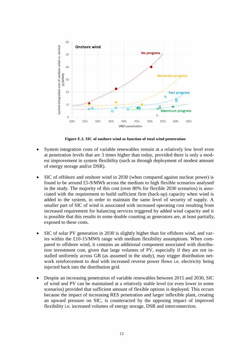
12
Figure E.3. SIC of onshore wind as function of total wind penetration
System integration costs of variable renewables remain at a relatively low level even
at penetration levels that are 3 times higher than today, provided there is only a mod-
est improvement in system flexibility (such as through deployment of modest amount
of energy storage and/or DSR).
SIC of offshore and onshore wind in 2030 (when compared against nuclear power) is
found to be around £5-9/MWh across the medium to high flexible scenarios analysed
in the study. The majority of this cost (over 80% for flexible 2030 scenarios) is asso-
ciated with the requirement to build sufficient firm (back-up) capacity when wind is
added to the system, in order to maintain the same level of security of supply. A
smaller part of SIC of wind is associated with increased operating cost resulting from
increased requirement for balancing services triggered by added wind capacity and it
is possible that this results in some double counting as generators are, at least partially,
exposed to these costs.
SIC of solar PV generation in 2030 is slightly higher than for offshore wind, and var-
ies within the £10-15/MWh range with medium flexibility assumptions. When com-
pared to offshore wind, it contains an additional component associated with distribu-
tion investment cost, given that large volumes of PV, especially if they are not in-
stalled uniformly across GB (as assumed in the study), may trigger distribution net-
work reinforcement to deal with increased reverse power flows i.e. electricity being
injected back into the distribution grid.
Despite an increasing penetration of variable renewables between 2015 and 2030, SIC
of wind and PV can be maintained at a relatively stable level (or even lower in some
scenarios) provided that sufficient amount of flexible options is deployed. This occurs
because the impact of increasing RES penetration and larger inflexible plant, creating
an upward pressure on SIC, is counteracted by the opposing impact of improved
flexibility i.e. increased volumes of energy storage, DSR and interconnection.

13
Sensitivity studies carried out for 2030 scenarios with a more ambitious carbon target
of 50 g/kWh suggest that the integration cost of variable RES would increase, driven
primarily by higher RES penetration required to meet the lower emission target. In
some instances, like in the Mid Flex and Onshore Capped scenarios where the pene-
tration of wind exceeds 55% of annual electricity demand, any integration of further
wind capacity becomes costly. Such high levels of wind require further improvements
in system flexibility or operation practices, such as those assumed in Modernisation or
Mega Flex scenarios.

14
1. Introduction
1.1. Background
With nearly half of UK’s generation capacity expected to retire in the build up to 2030, the
UK’s electricity system is facing exceptional challenges in the coming decades. Replacing
this generation capacity will for the most part need to be achieved with low-carbon electricity
generation technologies if we are to meet our carbon emission reduction targets and this will
need to be done whilst maintaining security of supply. Meeting the fourth carbon budget
(2023-27) will require that emissions are reduced by 50% on 1990 levels in 2025. The decar-
bonisation of electricity supply is also driven by the EU Renewables Directive, which stipu-
lates that the UK’s national share of energy from renewable sources in gross final consump-
tion in 2020 should reach 15%.
In order for the UK to meet its legally binding carbon targets through 2050, it will be critical
that the electricity sector makes large reductions to its carbon emissions by 2030, given its
potential for decarbonisation when compared to other energy subsectors. This will require
deployment of low-carbon generation technologies such as renewables, nuclear, biomass,
carbon capture and storage, etc. Despite the output variability that is a feature of some (pri-
marily renewable) low-carbon technologies, the decarbonised electricity system will need to
continue to operate at the same levels of security of supply that are considered acceptable to-
day.
One of the key challenges associated with decarbonisation is to ensure that electricity remains
affordable to consumers i.e. that the transition towards a low-carbon electricity supply is
achieved at the lowest possible cost for the society. This implies that it is critical to go be-
yond the pure LCOE estimates of individual low-carbon technologies and take into account
their whole-system costs when considering detailed operation and design of a power system
with high share of low-carbon generation. In that context, this work aims to provide evidence
that will contribute towards the delivery of a secure and decarbonised power sector at least
cost to consumers.
1.2. Concept of system integration costs of generation technologies
Understanding and quantifying the system integration costs (SICs) of various low-carbon
generation technologies (LCGTs) is important in the context of delivering a secure decarbon-
ised power sector at least cost in line with the legally binding 2050 decarbonisation targets
and security of supply imperatives. SICs of generation technologies (also sometimes referred
to as system externalities) include various types of costs that are imposed on the system by
added generation capacity, but which are not included in the capital or operating cost esti-
mates of these technologies. Examples of SIC components include:
Increased balancing cost associated with: a) increased requirements for system re-
serve due to higher uncertainty of variable renewable generation output, and
b) increased requirements for fast frequency regulation (response) due to reduced sys-
tem inertia.
Network reinforcements required in interconnection, transmission and distribution in-
frastructure (e.g. transmission reinforcement to connect remote wind resources or dis-

15
tribution network upgrade to cope with increased reverse power flows triggered by
high volume of distributed solar PV installations).
Increased backup capacity cost due to limited ability of e.g. variable renewable tech-
nologies to displace “firm” generation capacity needed to ensure adequacy of supply.
Cost of maintaining system carbon emissions, as the addition of certain technologies
may cause the overall emission performance of the system to deteriorate, requiring
that additional low-carbon capacity is installed to maintain the same level of carbon
emissions.
Some of these components, such as increased balancing or network cost may already be re-
flected to some extent in current charges imposed on generators, such as the balancing pay-
ments (BSUoS), or transmission and distribution charges (TNUoS and DUoS). Nevertheless,
it has been argued that these charges may not be fully cost-reflective11
, while on the other
hand some of the above components such as the backup capacity are not currently included in
LCOE assessments in any form.
The quantification of SICs in addition to the cost of building and operating low-carbon gen-
eration capacity, i.e. their Levelised Cost of Electricity (LCOE), therefore represents a critical
input into planning for a cost-effective transition towards a low-carbon electricity system,
enabling the development of policies and procurement mechanisms that consider both private
and wider system costs of different technologies. It also has to be noted that some compo-
nents of system integration costs are faced by generation plant owners in the market (such as
e.g. the impact of location on transmission charges), but many of them are not.
1.3. Challenges of integrating low-carbon generation
There are two key factors which may reduce the ability of the system to accommodate the
combination of inflexible low-carbon generation and variable renewables.
First, the expansion of variable renewables will lead to a significant increase in system bal-
ancing requirements in a low-carbon power system. Reserve requirements will increase due
to higher generation output fluctuations and consequently higher forecasting errors associated
with high RES penetrations. This is particularly relevant for wind generation, which is gener-
ally more difficult to predict than solar PV output. At the same time, given that solar PV and
wind represent non-synchronous power sources that tend not to contribute to system inertia,
the overall system inertia will decrease causing system frequency to fluctuate faster and more
widely during frequency incidents such as those caused by a sudden loss of generation.12
11 For a more detailed discussion on the issue, see a recent study prepared by NERA Economic Consulting and Imperial
College London for the Committee on Climate Change: “System integration costs for alternative low carbon generation
technologies – policy implications”, available here: https://www.theccc.org.uk/publication/system-integration-costs-for-
alternative-low-carbon-generation-technologies-policy-implications/.
12 It is noted that onshore and offshore wind turbines have the technical capability to provide “synthetic inertia” through
specifically designed control algorithms that ensure that in the event of a significant frequency drop their kinetic energy
is extracted and injected into the grid. Nevertheless, current regulatory framework does not require wind generators to
provide inertial response to the system.
16
Lower system inertia would in turn lead to higher requirements for primary frequency regula-
tion. The value of frequency regulation in the future GB system is hence expected to increase.
The need for reserve capacity and frequency regulation is also dependent on the size of the
largest credible generator loss in the system which would be the driven by deploying new
very large nuclear power stations.
Second, the present electricity system is characterised by relatively limited flexibility, mostly
provided by conventional gas and coal generation. Today’s generators are typically character-
ised by a limited amount of frequency control they can provide and a relatively high mini-
mum stable generation, and both of these features may represent limiting factors for the
amount of renewable generation that can be accommodated in the system. Conventional gen-
eration technologies with significantly enhanced flexibility are already available, but the lack
of appropriate market signals has so far suppressed their deployment. Similarly, energy stor-
age technologies and demand-side response could also significantly enhance system flexibil-
ity. It is important to mention that a tender for Enhanced Frequency Response (EFR) was re-
cently developed by National Grid to bring forward new technologies that support the decar-
bonisation of the energy industry by providing a fast response solution to system volatility. In
contrast to traditional frequency response delivered by conventional generation within ten
seconds, new class of technologies will enable the delivery of this response in under a second.
The operating cost associated with delivering energy is expected to decrease going forward as
the result of very low operating cost of most LCGTs. At the same time, the cost associated
with the provision of ancillary services is likely to increase substantially, driven by both in-
creased requirements for frequency regulation as well as the cost of managing the fluctua-
tions in variable LCGT output. Similarly, the volume of the capacity market is expected to
increase as historical generators retire and need to be replaced by more new capacity. The
increasing prominence of ancillary service and capacity markets should create opportunities
for flexible providers such as energy storage and DSR. Previous analysis by the authors
shows that the proportion of total system operating cost that can be attributed to ancillary ser-
vice provision would increase from about 2% today to more than 25% in the 2030 horizon,
driven by rapidly changing energy mix.
A more detailed discussion of challenges associated with the integration of variable renew-
ables is provided in Chapter 7, where a range of solutions is also described.
1.4. Key objective
In the context of the above, the main objective of this study is to first establish the likely level
of total system cost in the 2030 horizon across different scenarios, and then quantify and ex-
amine in more detail the SIC of low-carbon generation technologies such as nuclear, biomass,
variable renewable generation technologies, with particular focus on onshore and offshore
wind, in the context of the future, largely decarbonised UK electricity system.
For more details see e.g. F. M. Hughes, O. Anaya-Lara, N. Jenkins, and G. Strbac, “Control of DFIG-Based Wind Gen-
eration for Power Network Support”, IEEE Transactions on Power Systems, vol. 20, pp. 1958-1966, Nov. 2005.

17
2. Methodology for quantifying whole-system costs of low-carbon technologies
Most of the previous approaches to quantifying SICs focused on quantifying individual com-
ponents of SIC. All of these methods calculated the absolute integration cost i.e. the cost as-
sociated with a single technology that is added to the system. Nevertheless, there is at present
no commonly accepted method to quantify SIC, as different definitions have their own issues
with robustness or accuracy.
This report therefore focuses on quantifying the relative integration cost reflecting the differ-
ence between the system externalities of pairs of LCGTs. This approach ensures a robust cal-
culation approach while at the same time indicating relative merits of different LCGTs from
the whole-system perspective. In the studies presented in the report nuclear power is selected
as the counterfactual LCGT, against which the relative SIC of other LCGTs (wind, solar and
biomass) are quantified. The choice of nuclear as the benchmark technology is somewhat ar-
bitrary; however, this choice does not affect the differences between relative SICs quantified
for other LCGTs (such as e.g. between the SICs of wind and PV generation).
2.1. Whole-system assessment of electricity systems
Different components of SIC are incurred in different segments of the electricity system, such
as generation, transmission or distribution infrastructure, or are a part of system operation and
balancing cost. Therefore, the quantitative framework applied to evaluate the SIC is based on
the whole-system modelling approach i.e. the WeSIM model13
. This model has the ability to
simultaneously make investment and operation decisions with high (hourly) time resolution,
while capturing the interactions between different time scales (investment vs. short-term op-
eration) as well as across different asset types in the electricity system (e.g. generation vs.
network). At the same time the model can also consider various flexible technologies such as
energy storage or demand-side response (DSR). A distinct characteristic of the model is the
ability to capture and quantify the necessary investments in distribution networks in order to
meet demand growth and/or distributed generation uptake, based on the concept of statisti-
cally representative distribution networks. A detailed description of the model can be found
in the Appendix.
In this study the WeSIM model was applied to the interconnected GB electricity system that
was represented with four transmission nodes within GB and two neighbouring systems: Ire-
land and Continental Europe (CE), with the latter representing the entire interconnected
European system. In order to simulate cost-efficient outcomes across Europe, the model was
set up to optimise the operation of the entire European system, taking into account intercon-
nection capacities between systems. Two further important features endogenously included in
the model are the capability to impose a given carbon emission constraint for each system, as
well as ensure sufficient generation capacity is built in each system to meet the security of
supply standards.
13 D. Pudjianto, M. Aunedi, P. Djapic, G. Strbac, “Whole-Systems Assessment of the Value of Energy Storage in Low-
Carbon Electricity Systems”, IEEE Transactions on Smart Grid, vol:5, pp. 1098-1109, (2013).

18
2.2. Valuation of flexible options in future systems
As part of the whole-system assessment framework employed in this analysis, there are four
main categories of flexible options that were considered: (i) demand-side response (DSR),
(ii) flexible generation technologies, (iii) network solutions such as investing in interconnec-
tion, transmission and/or distribution networks, and (iv) the application of energy storage
technologies.14
Our previous study15
found that in the absence of alternative flexible balancing technologies
the scale of the balancing challenge in the future GB electricity system would increase very
significantly beyond 2030, with substantial investment needed in additional generation,
transmission and distribution assets to achieve the carbon emission targets while ensuring se-
curity of supply. Lack of flexibility significantly limits the system’s ability to integrate high
volumes of variable renewable energy sources (VRES): the same study demonstrated that up
to 30% of electricity theoretically available from VRES may need to be curtailed in 2050 if
no flexible options are deployed. VRES curtailment may become necessary to balance the
system, e.g. during periods of low demand, high renewable output, and high output of in-
flexible units such as nuclear plants, or conventional generators that have to be synchronised
in order to provide ancillary services. Curtailment of VRES will obviously have an adverse
impact on the carbon intensity of electricity supply given that the system effectively spills
zero-carbon renewable output. Additionally, curtailment of VRES would not necessarily be
predicated by a cost imperative, indicating that VRES is likely to be cheaper to curtail than
the alternative such as nuclear plant.
It is therefore essential to study various system flexibility levels as one of the key determi-
nants of the system’s ability to cost-effectively integrate VRES generation. Flexibility is
hence included as a key parameter in subsequent SIC studies as it is evident that flexibility
can greatly reduce the SIC of VRES, particularly in future development scenarios with high
shares of renewable generation.
2.3. Method for calculating SIC
The whole-system cost (WSC) of any generation technology can be expressed as the sum of
the LCOE of that technology and the corresponding SIC:
The cost terms in the above expression are typically expressed in monetary units per unit of
energy produced (e.g. in £/MWh). All generation technologies will potentially have a SIC
although for some technologies and systems this value may become negative (i.e. the tech-
nology may provide a system integration benefit). There is currently no widely accepted con-
14 Details on how these different flexible options have been included in the whole-system modelling framework can be
found in the recent CCC study: Imperial College London, “Value of Flexibility in a Decarbonised Grid and System Ex-
ternalities of Low-Carbon Generation Technologies”, report for the CCC, October 2015.
15 Imperial College London and NERA Economic Consulting, “Understanding the Balancing Challenge”, report for
DECC (2012).

19
sensus regarding the exact definitions of various components of SIC and their interactions,
and the methods for evaluating and allocating these costs vary considerably.16
In contrast to the approaches that quantify the components of SIC separately, such as e.g. by
considering only additional balancing or additional network cost without looking at their in-
teraction, this report quantifies the whole-system impact of adding a unit of LCGT in a given
system scenario while maintaining a given carbon intensity target. The approach presented
here quantifies each of the components of SIC that result from the system cost-optimally
adapting to the addition of LCGT across all cost categories. As an example, if there is a sig-
nificant volume of DSR present in low-voltage (LV) distribution grid, and wind capacity is
being added to the system requiring a higher volume of balancing services to be provided, it
may be opportune to invest into reinforcing the distribution network in order to enable the
system to access flexible DSR resource at the distribution level so that this flexibility can be
used to reduce balancing cost at the national level. These interactions and trade-offs would be
highly difficult to capture when quantifying SIC components separately.
In terms of the allowed response of the system to the addition of a unit of LCGT, we establish
a method to quantify the relative System Integration Cost that adopts nuclear power as the
benchmark LCGT, and is based on Method 2 elaborated in the earlier CCC study. The theo-
retical relationship between the relative SIC of technology 1 compared to technology 2, their
WSCs and LCOEs can be expressed as follows:17
Method 2, based on optimised replacement, assumes that 1 GW of nuclear capacity is re-
moved from the system, while the model is allowed to optimally increase the capacity of an-
other LCGT (e.g. wind or solar) while at the same time maintaining the same overall GB sys-
tem emissions. No change in the capacities of other LCGTs is allowed in this method; the
model is only allowed to adjust conventional capacity (CCGT and OCGT) if cost-efficient.
Changes in total system cost, excluding the investment and operation cost (i.e. LCOE) of the
pairs of technologies involved in the substitution (e.g. removed nuclear and added wind ca-
pacity), are divided by the annual output of the added low-carbon technology to establish its
relative SIC against nuclear power in £/MWh. Also, in this method any cost of LCGT capac-
ity added in excess of the energy-equivalent18
volume is factored into the total cost differen-
tial between the original system and a given SIC study.
16 An early meta-study comparing different approaches to quantifying the cost of integrating wind in the UK power sys-
tem was carried out by the UK Energy Research Council: “The Costs and Impacts of Intermittency – An assessment of
the evidence of the costs and impacts of intermittent generation on the British electricity network”, March 2006.
17 Note that this equation represents the theoretical relationship between whole-system costs, LCOEs and SICs. The actual
calculation method deployed in the study is elaborated in Section 3.6.2.
18 Energy equivalence here means that the removed and added capacities are capable of providing the same nominal an-
nual output (e.g. if the annual utilisation of nuclear is 90% and that of offshore wind is 43%, then it would take about
2.1 GW of wind capacity to produce the same output as 1 GW of nuclear).

20
3. Scenarios and assumptions
This chapter sets out the scenarios and other assumptions used to estimate the SIC of a range
of low-carbon generation technologies. Scenarios cover the period between 2015 and 2030,
with a single core scenario for years 2015, 2020 and 2025, and multiple scenarios for 2030
with varying degrees of flexibility as well as different low-carbon generation portfolios. This
study also includes a broad range of sensitivity analyses.
Given the decarbonisation agenda of the UK energy policy, all scenarios assume a significant
expansion of low-carbon generation capacity (i.e. nuclear and renewable, and to a lesser ex-
tent CCS capacity) between today and 2030. Also, the scenarios assumed a certain level of
targeted carbon intensity for the electricity system; in the basic set of studies this target was
set at 100 g/kWh in 2030, although sensitivity studies have been run with the 50 g/kWh target
as well.
3.1. Description of scenarios
A range of future development scenarios have been selected for this analysis based on the
Sponsors’ input, drawing upon recent DECC, CCC and National Grid scenarios. The time
horizon covered by the scenarios is until 2030. The following main scenarios are considered
in 2030:
1. Mid flexibility (“Mid Flex”): Central scenario with high wind deployment, reaching
up to 31 GW of offshore and 20 GW of onshore wind in 203019
. This scenario has
moderate levels of nuclear (8.2 GW), assuming the addition of 4.5 GW of new capac-
ity by 2030, and 20 GW of PV capacity. It also has a moderately high deployment
level of flexible options: 10 GW of new storage, 50% of DSR uptake and 11.3 GW of
interconnection capacity.
2. No progress (“No Flex”): Same as Mid Flex, but with no new storage, zero DSR up-
take and low interconnection capacity. With the regulated role out of smart meters and
significant cost benefits for any flexible system, this scenario should be seen as a use-
ful benchmark that informs the benefits of flexibility rather than as a viable scenario.
3. Low flexibility (“Low Flex”): Same as Mid Flex, but with less ambitious deployment
of flexible options: 5 GW of new storage, 25% DSR uptake and 10 GW of intercon-
nection.
4. Modernisation: Same as Mid Flex, but with a range of measures to improve system
operation (concerning wind predictability, capability to provide ancillary services
etc.).
19 Note that, as explained later, in the basic set of scenarios the offshore wind capacity was optimally reduced to reach the
given carbon intensity target (100 g/kWh).

21
5. High flexibility (“Mega Flex”): Scenario with similar generation mix as the Mid Flex
scenario, but with enhanced flexibility i.e. higher storage (15 GW) and interconnec-
tion capacity (15 GW) and greater DSR uptake than the Mid Flex (100%).
6. Onshore Capped: Scenario with no new onshore wind deployment beyond today’s
level20
(around 8 GW), but compensated by a more intensive expansion of offshore
wind (up to 39 GW) until 2030. Nuclear and PV capacity are at the Mid Flex level.
7. Nuclear Centric: This represents a theoretical alternative technological solution to a
high variable LCGT mix for achieving the UK’s decarbonisation agenda. Whilst a
more ambitious nuclear expansion in this scenario (16.4 GW in 2030) seems un-
achievable to deliver from today’s perspective, this scenario nevertheless offers a use-
ful benchmark to assess the cost-effectiveness of an energy mix with high levels of
variable LCGT. The scenario therefore has slower wind development (up to 21 GW of
offshore and 12.5 GW of onshore wind, compared to 5.1 GW of offshore and 9 GW
of onshore today).
The Mid Flex scenario is also backtracked to include years 2015, 2020 and 2025, and is also
referred to as “Base Case” in those years. Other scenarios only referred to 2030 (although
sensitivity studies on system flexibility were also carried out for 2020 and 2025, as explained
in Section 6.3).
3.2. Assumptions on generation technologies
3.2.1. Generation capacity
Table 3.1 provides an overview of the assumed starting generation capacities across all sce-
narios. Generation mixes for No Flex, Low Flex, Modernisation and Mega Flex scenarios
were the same as in the Base Case scenario.
20 This scenario reflects the uncertain future evolution of offshore wind in light of the recent closure of the Renewables
Obligation (RO) to onshore wind capacity in Great Britain that took effect on 12 May 2016.

22
Table 3.1. Generation capacity assumptions across scenarios (in GW)
Scenario name
Basecase 15 Basecase 20 Basecase 25 Mid Flex* Onshore capped
Nuclear centric
Year 2015 2020 2025 2030 2030 2030
Nuclear 9.4 8.9 7.9 8.2 8.2 16.4
Gas CCGT** 29.3** 29.3** 18.0** 16.0** 16.0** 16.0**
Coal 18.7 10.9 - - - -
Gas CCS - - 0.5 0.5 0.5 0.5
Onshore 9.0 13.2 16.6 20.0 8.0 12.5
Offshore*** 5.1 10.2 16.2 31.0*** 39.0*** 21.0***
Solar 8.8 12.8 16.4 20.0 20.0 20.0
Biomass 4.0 3.4 3.4 3.4 3.4 3.4
Hydro 1.5 1.5 1.5 1.5 1.5 1.5
Pumped st. 2.8 2.8 3.7 3.7 3.7 3.7
Notes: * The same starting generation mix as in Mid Flex scenario was also assumed in No Flex, Low Flex, Modernisa-tion and Mega Flex scenarios. ** CCGT capacity in the table represents the legacy capacity that would be in place without any new CCGT plants. The model was allowed to build more CCGT if cost-effective. *** In the core scenario runs the offshore wind capacity in 2030 was subject to cost-optimal reduction while meet-ing the system-level carbon target of 100 g/kWh.
As indicated in the table, capacities of certain technologies were modified by the model when
finding a least-cost solution. CCGT capacity was optimised on top of the capacity of current
generators that will still be in operation until 2030. With offshore wind capacity, the capacity
was reduced in a cost-optimal fashion in order to meet the 100 g/kWh target in 2030.21
In the
modelling OCGT generation is used as a proxy for peaking capacity that may be required to
enforce the security of supply criterion, as the low capital cost and high utilisation cost of
OCGT are representative of a typical peaking unit. In reality OCGT could be replaced with
distributed reciprocating engines, CCGTs, storage or DSR if these where perceived as
cheaper or more desirable alternatives. .
3.2.2. Capacity factors
Table 3.2 sets out the assumptions on achievable capacity factors for different generation
technologies across time. Note that all 2030 scenarios had the same capacity factor assump-
tions. All other technologies (e.g. conventional plant) had their utilisation factors determined
by the model as the result of optimisation.
21 According to preliminary studies carried out, without this reduction the Base Case system would be able to achieve
carbon intensities of below 60 g/kWh, i.e. would over-deliver on the carbon target due to abundant low-carbon genera-
tion capacity.

23
Table 3.2. Maximum22
capacity factors of generation technologies across scenarios
Year 2015 2020 2025 2030
Nuclear* 66% 66% 73% 90%
Gas CCS 90% 90% 90% 90%
Onshore wind 30% 30% 30% 30%
Offshore wind 47% 47% 47% 47%
Solar 11% 11% 11% 11%
Biomass** 75-90% 75-90% 75-90% 90%
Notes: * Nuclear capacity factors in different years are based on historical data on the utilisation of existing plant com-bined with the expected utilisation of new nuclear units. ** Biomass generation in years 2015, 2020 and 2025 had a specified minimum utilisation of 75% in our studies, as it would otherwise see very low utilisation due to high operating cost in the absence of support mechanisms.
The evolution of nuclear capacity factors over time is a blend of relatively lower utilisation
achieved by currently existing plants (some of which have technical issues that prevent them
from operating at full output) and high utilisation (~90%) of new nuclear units.
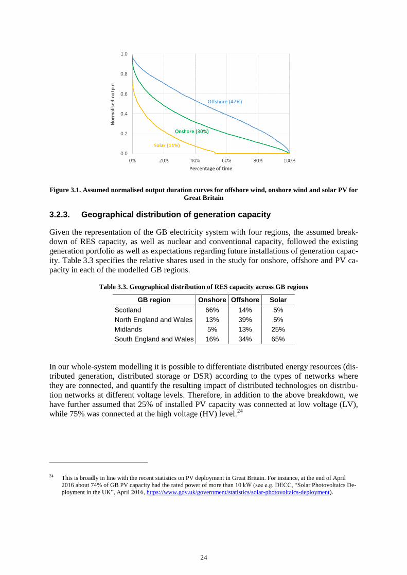
Capacity factors of onshore and offshore wind are based on the Sponsors’ estimates, while
the PV utilisation is taken from the 2015 version of DECC’s energy projections23
. These ca-
pacity factors have been supported by regional hourly output profiles for wind and PV gen-
erators, which Imperial have developed in previous analyses. The hourly RES output profiles
were further differentiated according to four GB regions used in the modelling, so that for
instance an onshore wind generator in Scotland has a higher utilisation factor than onshore
wind located in South England. Conversely, the utilisation of PV generation is higher in the
south than in the north of Great Britain. Figure 3.1 presents the normalised output duration
curves for UK-representative wind and PV profiles used in the study.
22 Maximum in the context of wind and PV generation refers to maximum achievable load factor; if there is curtailment of
variable RES output, the actual utilisation of these technologies could be lower.
23 Department of Energy and Climate Change, “Updated energy and emissions projections: 2015”, available at:
https://www.gov.uk/government/publications/updated-energy-and-emissions-projections-2015.
24
Figure 3.1. Assumed normalised output duration curves for offshore wind, onshore wind and solar PV for
Great Britain
3.2.3. Geographical distribution of generation capacity
Given the representation of the GB electricity system with four regions, the assumed break-
down of RES capacity, as well as nuclear and conventional capacity, followed the existing
generation portfolio as well as expectations regarding future installations of generation capac-
ity. Table 3.3 specifies the relative shares used in the study for onshore, offshore and PV ca-
pacity in each of the modelled GB regions.
Table 3.3. Geographical distribution of RES capacity across GB regions
GB region Onshore Offshore Solar
Scotland 66% 14% 5%
North England and Wales 13% 39% 5%
Midlands 5% 13% 25%
South England and Wales 16% 34% 65%
In our whole-system modelling it is possible to differentiate distributed energy resources (dis-
tributed generation, distributed storage or DSR) according to the types of networks where
they are connected, and quantify the resulting impact of distributed technologies on distribu-
tion networks at different voltage levels. Therefore, in addition to the above breakdown, we
have further assumed that 25% of installed PV capacity was connected at low voltage (LV),
while 75% was connected at the high voltage (HV) level.24
24 This is broadly in line with the recent statistics on PV deployment in Great Britain. For instance, at the end of April
2016 about 74% of GB PV capacity had the rated power of more than 10 kW (see e.g. DECC, “Solar Photovoltaics De-
ployment in the UK”, April 2016, https://www.gov.uk/government/statistics/solar-photovoltaics-deployment).

25
3.2.4. Cost assumptions
The levelised cost of energy (LCOE) assumptions for different technologies were mostly
based on DECC’s 2013 generation cost update.25
There is strong evidence, even from the
Government itself, that this data set is outdated; we have therefore used alternative cost data
sources for certain technologies where available, as specified in Table 3.4 below. The as-
sumptions in different scenarios follow the rationale where e.g. higher deployment of off-
shore wind or nuclear generation leads to a reduction in cost of the technology.
Table 3.4. LCOE assumptions for selected technologies across scenarios (in £/MWh, real 2015 prices)
Scenario name Basecase 15 Basecase 20 Basecase 25 Mid Flex Onshore capped
Nuclear centric
Year 2015 2020 2025 2030 2030 2030
Nuclear 93 93 90 90 90 80
Gas CCS - - 122 123 123 123
Onshore wind26
75 65 60 60 60 60
Offshore wind27
133 106 80 75 70 80
Solar28
101 86 75 65 65 65
Biomass 108 108 108 108 108 108
LCOE assumptions in No Flex, Low Flex, Modernisation and Mega Flex scenarios were
identical to those made for the Mid Flex scenario.
3.3. Demand assumptions
Projected demand for years 2015 to 2030 used in the study has been based on the CCC sec-
toral scenario for the electricity sector29
, which supported the drafting of the Fifth Carbon
Budget. The baseline (Other) demand in this scenario is projected to remain broadly similar,
with a slowly declining trend beyond 2020. On the other hand the uptake of electrified trans-
25 DECC, “Electricity generation costs”, July 2013, available at:
https://www.gov.uk/government/uploads/system/uploads/attachment_data/file/223940/DECC_Electricity_Generation_
Costs_for_publication_-_24_07_13.pdf.
26 Sources:
1) Renewable UK, “Onshore Wind Cost Reduction Taskforce Report”, April 2015,
http://www.renewableuk.com/en/publications/reports.cfm/Onshore%20Wind%20Cost%20Reduction%20Taskforce%20
Report
2) Policy Exchange, “Powering Up: The future of onshore wind in the UK”, 2015,
http://www.policyexchange.org.uk/images/publications/powering%20up.pdf
27 Source: BVG Associates, “Approaches to cost reduction in offshore wind”, report for the CCC, 2015,
https://www.theccc.org.uk/publication/bvg-associates-2015-approaches-to-cost-reduction-in-offshore-wind/.
28 Sources:
1) KPMG, “UK solar beyond subsidy: the transition”, report for REA, July 2015, http://www.r-e-a.net/upload/uk-solar-
beyond-subsidy-the-transition.pdf.
2) Solar Trade Association, “Cost reduction potential of large scale solar PV”, November 2014, http://www.solar-
trade.org.uk/wp-content/uploads/2015/03/LCOE-report.pdf.
29 Climate Change Committee, “Sectoral scenarios for the fifth carbon budget – Technical report”, November 2015,
https://www.theccc.org.uk/publication/sectoral-scenarios-for-the-fifth-carbon-budget-technical-report/.

26
port and heating in the domestic sector is projected to increase from about zero today to
around 21 TWh and 9 TWh, respectively. The evolution of demand is provided in Table 3.5.
Table 3.5. Projected electricity demand between 2015 and 2030 (in TWh)
Year 2015 2020 2025 2030
Domestic Heat (HP) 0.6 2.1 5.0 9.0
Electric Vehicles 0.1 1.3 7.0 21.0
Losses 26.0 26.0 26.5 27.0
Other 302.3 305.1 302.6 298.0
Total 329 335 341 355
A single projection was made for each year, therefore all 2030 scenarios had the same de-
mand assumptions.
3.4. Flexibility assumptions
3.4.1. Deployment of flexible options
Key assumptions regarding the assumed deployment of flexible options across different sce-
narios are given in Table 3.6. Onshore Capped and Nuclear Centric scenarios are omitted as
they had the same flexibility assumptions as the Mid Flex scenario.
Table 3.6. Deployment of flexible options across scenarios
Scenario name Basecase
15 Basecase
20 Basecase
25 No Flex Low Flex Mid Flex*
Moderni-sation**
Mega Flex
Year 2015 2020 2025 2030 2030 2030 2030 2030
New storage (GW)
0 0.2 2 0 5 10 10 15
DSR 0% 0% 25% 0% 25% 50% 50% 100%
Interconnection (GW)
4.0 7.5 11.3 7.5 9.9 11.3 11.3 15.0
* Onshore Capped and Nuclear Centric scenarios had the same flexibility assumptions as the Base Case. * The Modernisation scenario had the same deployment of storage, DSR and interconnection as the Base Case, but included improved system operation practices as detailed in Section 3.4.2.
New energy storage (in addition to the projected capacity of pumped storage in Table 3.1) is
assumed to be available in distributed form similar to battery storage. Its capacity is increased
from broadly zero today to between 0 and 15 GW in 2030 scenarios. It was further assumed
that new storage would be sufficiently fast-responding to be able to provide frequency re-
sponse to the system operator.30
The assumed duration of energy storage (i.e. the ratio be-
tween the maximum energy stored and installed power) was 5 hours, so that for instance
5 GW of storage capacity was assumed to be able to store 25 GWh of energy.
30 This is in line with recent developments of new ancillary service products by National Grid, such as Enhanced Fre-
quency Response that requires sub-second response times; this service is primarily targeting battery providers.

27
The uptake of demand-side response (DSR) is assumed to increase from around zero in 2020
to 50% in 2030 in the Base Case scenario. The 2030 DSR uptake varied between 0% in the
No Flex to full uptake in the Mega Flex. The DSR potential is quantified based on our previ-
ous bottom-up modelling of different flexible demand categories, which considered how they
perform their actual functions while exploiting the flexibility that may exist without compro-
mising the service delivered to end users. In our modelling we differentiated between four
types of potentially flexible demand:
Electric vehicles: up to 80% of EV demand could be shifted away from a given hour
to other times of day;
Heat pumps: heat storage enables that the 35% of HP demand can be shifted from a
given hour to other times of day;
Smart appliances: demand attributed to white appliances (washing machines, dish-
washers, tumble dryers) participating in smart operation can be fully shifted away
from peak;
Industrial and commercial demand: 10% of the demand of I&C customers participat-
ing in DSR schemes can be redistributed.
The above assumptions correspond to 100% DSR uptake i.e. represent the maximum achiev-
able potential. The actual DSR availability is scaled down according to the assumed DSR up-
take level (e.g. the 50% DSR uptake assumes that only half of the theoretical potential is real-
ised).
Interconnection capacity is projected to increase from the current 4 GW to 11.3 GW in 2030
(Mid Flex), assuming the realisation of currently approved and planned interconnection pro-
jects. Available interconnection capacity was varied across different flexibility scenarios,
from 7.5 GW in No Flex to 15 GW in the Mega Flex scenario.
3.4.2. Improved system operation in Modernisation scenario
There is a number of different possibilities as to how the system operation practices in the
future may become more flexible and more efficient, in particular with respect to the man-
agement of wind generation. In this report we have modelled several of these improvements
that were deemed of particular interest, but this by no means implies these are the only possi-
bilities.
The improvements in system operation assumed in the Modernisation scenario included:
Wind generators being able to provide synthetic inertia and frequency response
Wind installations are normally realised through non-synchronous generation tech-
nologies, which cannot provide inertia unless equipped with advanced control
schemes. Although theoretical solutions are available in scientific literature, wind
generators are currently not required to provide system inertia. With higher wind
penetrations, it may become opportune to improve the control of wind generators to
enable them to contribute to system inertia similar to conventional plant that they are
likely to displace in future electricity mix.

28
Wind generators being able to provide reserve when curtailed
In the future system with high wind penetration it may become necessary to occasion-
ally curtail wind or PV output in situations of excess available energy and low de-
mand. Curtailed renewable output may in those situations be used to provide reserve
services to the system operator and potentially replace reserve provided by conven-
tional units. More generally, wind generators that can access reserve and balancing
markets may choose to curtail their output whenever the value of reserve or balancing
service exceeds the value obtained from the wholesale market. This option is not util-
ised today given the current market structure and low frequency of curtailment events,
but it may become more commonplace in future.
Improved forecasting of wind
There is continuous improvements in wind forecasting techniques which may eventu-
ally lead to reduced reserve requirements, as the forecasting error which the system
operator needs to be able to resolve would become lower and hence require less re-
serve service to be procured.
Ability to procure frequency response services via interconnectors
This option is also not commonly used in today’s systems, but with increased fre-
quency response requirements it may become beneficial to use interconnection capac-
ity not only to enable energy exchanges, but also to facilitate trading of balancing ser-
vices.
3.5. Other assumptions
3.5.1. Carbon intensity target
In this study we imposed an explicit carbon intensity target of 100 g/kWh in 2030 across the
main set of scenarios. No carbon target was specified for 2015, 2020 or 2025. The 100 g/kWh
target is often considered as an appropriately ambitious intermediate decarbonisation goal on
the pathway to achieve the 2050 carbon reduction target.31
As explained later in the report, we also analysed the performance of the system in an addi-
tional set of sensitivity studies that assumed a more ambitious 2030 target of 50 g/kWh.
3.5.2. Fuel and carbon prices
Summary of fuel and carbon price assumptions over the study period is given in Table 3.7.
Table 3.7. Projected fuel and carbon prices between 2015 and 2030
Year 2015 2020 2025 2030
Coal ($/tonne) 57.3 66.3 79.1 83.2
Gas (p/therm) 37.5 28.8 36.9 45.0
Carbon (£/t) 5.9 6.6 22.6 47.1
31 See for instance the CCC Fifth Carbon Budget.

29
The key source for fuel and carbon price projections is DECC’s 2015 update of energy and
emissions projections32
. Coal and carbon33
price projections follow the Reference price sce-
nario, while the gas price evolution is taken from the Low Prices scenario34
.
3.5.3. System security assumptions
The GB system in our modelling was required to maintain sufficient firm capacity margin
over peak demand to ensure that the specified reliability standard is complied with. The reli-
ability criterion used is the Loss of Load Expectation (LOLE), which was limited at 3 hours
per year35
. The appropriate level of LOLE is directly linked to the Value of Lost Load
(VOLL) that the customers are assumed to place on having their demand met. This relation-
ship is rather complex as VOLL generally depends on customer type, size, location, time of
day etc. however it is normally assumed that VOLL is in the order of several thousand
pounds (at present VoLL at £17,000/MWh is used in the Capacity Market). With the rollout
of smart meters and higher DSR uptake levels the flexibility in terms of shifting demand or
providing system services will increase significantly, however, it is likely that the customers
will still place a very high value on the inflexible part of their demand.
With high levels of heating demand electrification the peak demand would become even
more sensitive to the severity of cold winter conditions. In the study we assumed that peak
demand would correspond to a normal (i.e. average) winter rather than the coldest 1-in-20
winters (as was assumed in some of the previous system studies). In practice, assuming a 1-
in-20 cold winter would result in a higher system peak demand and hence higher requirement
for peaking (OCGT) capacity. A large proportion of this capacity would be very seldom used
i.e. would be characterised by very low utilisation factors. Nevertheless, having this capacity
available and therefore ensuring a sufficient capacity margin is necessary to maintain the se-
curity of supply. Our previous studies have shown that assuming a higher peak demand
driven by extreme winter weather would have no material impact on SIC of LCGTs, which is
the core objective of this study.
3.5.4. Interaction with neighbouring systems
In order to ensure that the GB system is largely self-reliant, and to avoid distorting the system
carbon intensity evaluation when importing or exporting significant volumes of electricity,
we further impose an energy neutrality constraint for the GB system. This means that energy
flows over interconnectors with neighbouring systems are constrained to ensure Britain is
“energy neutral”, i.e. that total TWh of energy demand over the year equals total production
from British generators. Therefore, while the model can use interconnectors to support sys-
tem balancing at any point of time, the model will ensure the energy neutrality constraint is
respected on an annual basis.
32 DECC, “Updated energy and emissions projections: 2015”, https://www.gov.uk/government/publications/updated-
energy-and-emissions-projections-2015.
33 Carbon price projection assumed is the one applicable for Industry and Services. This is the projection for traded carbon
price under the EU Emissions Trading Scheme.
34 This approach was taken in light of the recent significant drop in gas prices.
35 The LOLE of 3 hours is consistent with the level of security targeted in the British Capacity Mechanism.
30
The topology of the system used in the study requires that assumptions on generation, de-
mand etc. are also made for the two neighbouring systems (Ireland and Continental Europe).
We therefore assume the generation and demand background for the European system that
reflects the decarbonisation and RES expansion resulting from recent European climate
change policies36
. Decarbonisation of heating and transport is assumed to evolve at similar
proportions to those assumed for the GB system. Also, the assumed DSR uptake in Europe is
consistent with the DSR uptake in Britain. The assumed carbon and fuel prices in GB were
also assumed to apply in the rest of Europe.
3.6. Optimisation set-up for scenarios and SIC studies
This section explains how we constructed the counterfactual scenarios based on initial sce-
nario assumptions in Table 3.1, and later used these counterfactual as a foundation for run-
ning SIC studies.
3.6.1. Counterfactual scenarios
Starting from the scenarios specified in Table 3.1, the counterfactuals were established by
optimising the following components of the scenarios:
OCGT capacity was optimised from zero. Note that OCGT in this context as used as
proxy for flexible peaking capacity. If there was another technology with lower in-
vestment cost (such as e.g. gas reciprocating engines), then it could be substituted for
OCGT in subsequent discussion.
CCGT capacity was optimised from the minimum level for each year as specified in
Table 3.1.
In 2030 scenarios, subject to carbon target, the offshore wind capacity was allowed to
reduce as part of the optimisation while the model was required to meet the
100 g/kWh carbon intensity target.
In all scenarios that envisage new storage capacity (see Table 3.6) this capacity was
optimally allocated between five37
GB regions, as well as between different distribu-
tion network types (urban, rural or intermediate) in each region.
In all scenarios the model was allowed to add more interconnection capacity (at a
cost) if cost-efficient.38
The summary of model outputs in terms of added or reduced capacities in counterfactual sce-
narios is provided in Table 3.8 for years between 2015 and 2030 (with the Base Case scenario
36 Imperial College London, NERA Economic Consulting, DNV GL, “Integration of Renewable Energy in Europe”, June
2014, https://ec.europa.eu/energy/sites/ener/files/documents/201406_report_renewables_integration_europe.pdf.
37 In terms of distribution network and demand representation, London was considered as a separate, fifth region. In terms
of transmission topology, London was embedded within the South England and Wales region.
38 This was allowed to ensure feasibility of model runs. As shown later in the report, in a large majority of cases the model
did not add any new interconnection capacity.

31
included for 2030), and in Table 3.9, where the capacities are reported across different 2030
scenarios.
Table 3.8. Capacity of optimised technologies in counterfactual Base Case scenarios between 2015 and
2030 (in GW)
Scenario name Basecase 15 Basecase 20 Basecase 25 Mid Flex
Year 2015 2020 2025 2030
OCGT 8.1 19.6 29.9 30.0
New CCGT* - 0.1 3.9 0.1
Offshore wind 5.1 10.2 16.2 22.2
Reduced wind** - - - -8.8
Notes: * CCGT capacity added on top of the capacity in Table 3.1. ** Reduction compared to the initial capacity in Table 3.1.
Note that in the No Flex scenario the model was used to optimally add CCS capacity, as the
original capacities of wind and other LCGTs was insufficient to meet the 100 g/kWh target.
Table 3.9. Capacity of optimised technologies in 2030 counterfactual scenarios (in GW)
Scenario name No Flex Low Flex Mid Flex Moderni-
sation Mega Flex
Onshore capped
Nuclear centric
OCGT 41.7 38.2 30.0 30.1 20.2 30.0 21.9
New CCGT* 9.3 1.6 0.1 0.1 - 0.1 0.1
Offshore wind 31.0 23.1 22.2 21.7 21.5 29.9 11.3
Reduced wind**
- -7.9 -8.8 -9.3 -9.5 -9.1 -9.7
Added CCS 2.1 - - - - - -
Notes: * CCGT capacity added on top of the capacity in Table 3.1. ** Reduction compared to the initial capacity in Table 3.1.
Along with the capacities i.e. investment decisions, all model runs for counterfactual scenar-
ios also provided optimal decisions with respect to operation of the system, resulting in a cer-
tain level of operating cost associated with the use of fuel and the resulting carbon emissions.
3.6.2. System Integration Cost studies
With the counterfactual scenarios established as shown in Table 3.8, the system integration
cost studies were set up in line with the approach described in Section 2.3, i.e. using the fol-
lowing steps:
1 GW of nuclear capacity was removed from each counterfactual scenario, and an en-
ergy-equivalent amount of another LCGT added to retain the same nominal amount of
low-carbon electricity available in the system.39
Given that the utilisation of nuclear
portfolio varied across different years, the energy-equivalent capacities also changed
39 The energy-equivalent capacity in GW to replace 1 GW of nuclear is simply the inverse of the ratio of the achievable
utilisation factors of a given LCGT and nuclear, as specified in Table 3.2.

32
as specified in Table 3.10. Note that one SIC study is required for each scenario and
each of the four LCGTs.
Table 3.10. Energy-equivalent capacity additions for different LCGTs (in GW) when removing 1 GW of
nuclear power
Year 2015 2020 2025 2030
Offshore wind 1.40 1.40 1.55 1.91
Onshore wind 2.33 2.33 2.58 3.18
Solar PV 5.93 5.93 6.56 8.09
Biomass 0.88 0.88 0.97 1.00
For each 2030 scenario, the system was required to maintain the 100 g/kWh carbon
intensity target following the replacement of nuclear with another LCGT. The model
was allowed to add further LCGT capacity (above the energy-equivalent amount) if
needed to keep the emissions at 100 g/kWh.
The model was also allowed to re-optimise OCGT and new CCGT capacity, as well
as all decisions regarding system operation. Capacities of all other LCGTs, intercon-
nection and storage were kept constant.
The difference in total system cost (investment in generation and network infrastruc-
ture plus operating cost) before and after the replacement is then interpreted as the
relative integration cost between nuclear and a given LCGT. It has to be noted that
this cost difference should not include the LCOEs associated with the energy equiva-
lent capacities of nuclear and the other LCGT that replaces it; however, any invest-
ment cost associated with installing additional LCGT capacity above the energy-
equivalent volume is calculated into the cost difference as it arises from the lower
ability of the system to absorb the LCGT in question. If the cost of the system after
replacement was higher, the LCGT in question had a positive SIC (and vice versa).
Dividing the cost differential with the replaced annual nuclear output finally provides
us with the measure of relative integration cost of each LCGT compared to nuclear,
expressed in £/MWh.
To make results comparable and consistent, all capacity additions and removals imposed in
the SIC studies were assumed to occur in South of GB.
33
4. System Integration Costs of low-carbon technologies
This chapter discusses the results of quantitative case studies to determine SIC of LCGTs
when a small amount of them is added to the system. The broad range of scenarios analysed
demonstrates that the integration cost of LCGTs is a function of the system they are being
added to, heavily dependent in particular on the volume of low-carbon capacity already pre-
sent in the system and flexibility level in the system. The results of SIC studies presented
here are disaggregated across key components: generation, transmission and distribution in-
vestment cost (CAPEX) as well as operating cost (OPEX). G CAPEX and OPEX components
are further broken down by technologies to identify where different components of integra-
tion cost originate.
As discussed before, the SIC results presented in this chapter refer to relative integration cost
of LCGTs when compared against nuclear generators. To aid comparison, the assumed
LCOE differentials (i.e. cost advantages) of different LCGTs against nuclear are also referred
to in the text. If the relative integration cost for a given technology is higher than its corre-
sponding LCOE cost advantage against nuclear, this suggests that a unit of this technology
provides a lower net marginal benefit to the system than a unit of nuclear capacity.
4.1. Counterfactual scenarios
Section 3.6.1 explained how the counterfactual scenarios used in this study have been ob-
tained, i.e. which variables were optimally determined by running the WeSIM model. This
section provides more details on the results of these counterfactual scenarios, specifically the
generation capacity portfolios, generator outputs and capacity factors across different years
and scenarios.
4.1.1. Optimised generation portfolios
As explained earlier, in all 2030 scenarios the model was used to optimally add peaking
(OCGT40
) and CCGT capacity, while at the same time removing offshore wind capacity
while still being able to meet the 100 g/kWh carbon intensity target. The exception to this
was the No Flex scenario, where the volume of LCGTs was not sufficient to deliver the
100 g/kWh intensity, so the model was used to add CCS capacity to meet the carbon target.
Capacities of other generation technologies were given as part of scenario assumptions. Gen-
eration mix in 2015 was constructed so as to reflect the currently existing GB generation
portfolio.
Figure 4.1 presents the composition of the counterfactual generation mixes obtained across
Base Case scenarios between 2015 and 2030. As evident from the figure, the 2030 scenarios
assume a gradual decline in coal capacity, accompanied by a rapid increase in low-carbon
generation, particularly wind and PV. The Base Case scenarios also feature a steadily increas-
ing energy storage capacity compared to today’s levels. Finally, the capacity of peaking i.e.
40 As noted earlier, the role of peaking capacity assumed by OCGT in this study could be taken on by another generation
or storage technology should its cost be considered more attractive than that of OCGT generation.
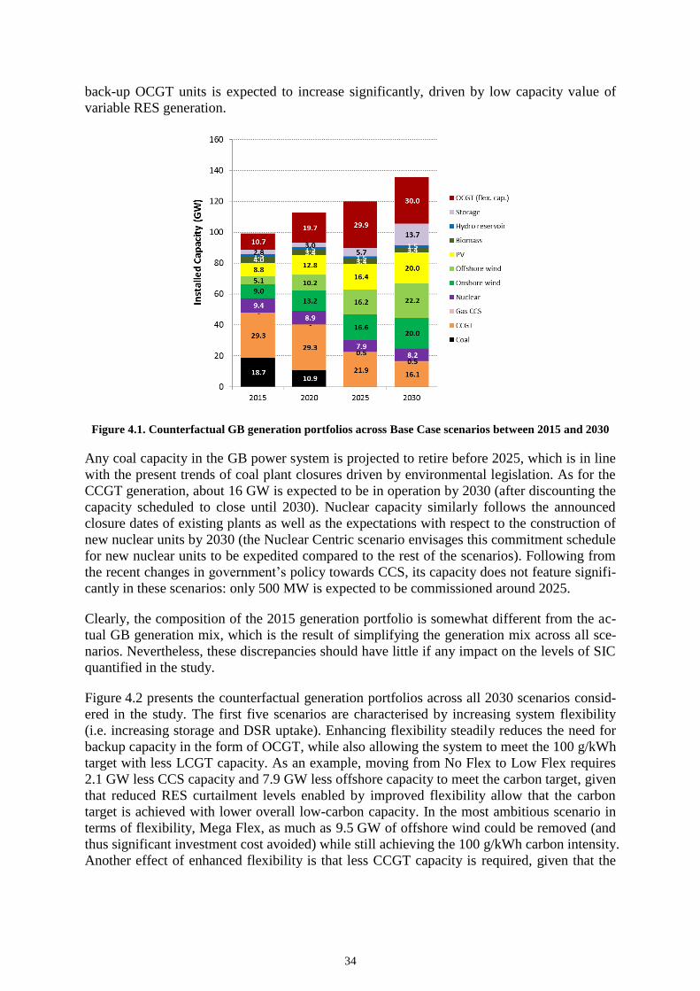
34
back-up OCGT units is expected to increase significantly, driven by low capacity value of
variable RES generation.
Figure 4.1. Counterfactual GB generation portfolios across Base Case scenarios between 2015 and 2030
Any coal capacity in the GB power system is projected to retire before 2025, which is in line
with the present trends of coal plant closures driven by environmental legislation. As for the
CCGT generation, about 16 GW is expected to be in operation by 2030 (after discounting the
capacity scheduled to close until 2030). Nuclear capacity similarly follows the announced
closure dates of existing plants as well as the expectations with respect to the construction of
new nuclear units by 2030 (the Nuclear Centric scenario envisages this commitment schedule
for new nuclear units to be expedited compared to the rest of the scenarios). Following from
the recent changes in government’s policy towards CCS, its capacity does not feature signifi-
cantly in these scenarios: only 500 MW is expected to be commissioned around 2025.
Clearly, the composition of the 2015 generation portfolio is somewhat different from the ac-
tual GB generation mix, which is the result of simplifying the generation mix across all sce-
narios. Nevertheless, these discrepancies should have little if any impact on the levels of SIC
quantified in the study.
Figure 4.2 presents the counterfactual generation portfolios across all 2030 scenarios consid-
ered in the study. The first five scenarios are characterised by increasing system flexibility
(i.e. increasing storage and DSR uptake). Enhancing flexibility steadily reduces the need for
backup capacity in the form of OCGT, while also allowing the system to meet the 100 g/kWh
target with less LCGT capacity. As an example, moving from No Flex to Low Flex requires
2.1 GW less CCS capacity and 7.9 GW less offshore capacity to meet the carbon target, given
that reduced RES curtailment levels enabled by improved flexibility allow that the carbon
target is achieved with lower overall low-carbon capacity. In the most ambitious scenario in
terms of flexibility, Mega Flex, as much as 9.5 GW of offshore wind could be removed (and
thus significant investment cost avoided) while still achieving the 100 g/kWh carbon intensity.
Another effect of enhanced flexibility is that less CCGT capacity is required, given that the
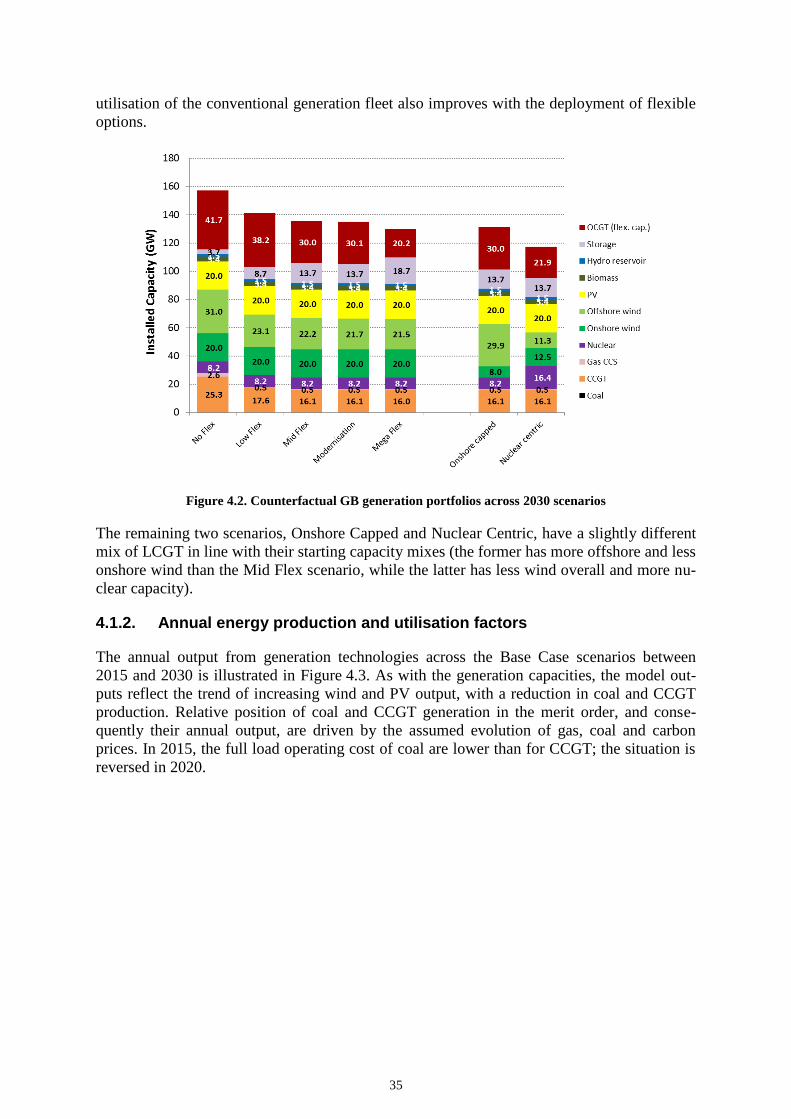
35
utilisation of the conventional generation fleet also improves with the deployment of flexible
options.
Figure 4.2. Counterfactual GB generation portfolios across 2030 scenarios
The remaining two scenarios, Onshore Capped and Nuclear Centric, have a slightly different
mix of LCGT in line with their starting capacity mixes (the former has more offshore and less
onshore wind than the Mid Flex scenario, while the latter has less wind overall and more nu-
clear capacity).
4.1.2. Annual energy production and utilisation factors
The annual output from generation technologies across the Base Case scenarios between
2015 and 2030 is illustrated in Figure 4.3. As with the generation capacities, the model out-
puts reflect the trend of increasing wind and PV output, with a reduction in coal and CCGT
production. Relative position of coal and CCGT generation in the merit order, and conse-
quently their annual output, are driven by the assumed evolution of gas, coal and carbon
prices. In 2015, the full load operating cost of coal are lower than for CCGT; the situation is
reversed in 2020.

36
Figure 4.3. Annual outputs of GB generators across Base Case scenarios between 2015 and 2030
Figure 4.4 illustrates the generation outputs across the counterfactual 2030 scenarios with
varying flexibility and generation mixes. The share of annual electricity demand met by wind
generation increases to about 40% in most 2030 scenarios (with the exception of Nuclear
Centric). In the same scenarios, when all renewable technologies are added together (wind,
PV, biomass and hydro), their share in meeting the electricity demand reaches around 55%. It
can be observed that in the No Flex scenario the capacity factors of wind and PV are lower
than in other scenarios due to significant output curtailment (in the order of 10% of annually
available energy).
Figure 4.4. Annual outputs of GB generators across 2030 counterfactual scenarios

37
Annual utilisation of generation technologies in counterfactual Base Case scenarios over the
period 2015-2030 is given in Table 4.1. Note that the actual observed utilisation factors of
renewable technologies, nuclear and CCS generation are bounded by the assumed achievable
capacity factors specified in Section 3.2.2. The last row of the table also provides the ob-
served carbon intensity of GB electricity supply across scenarios (note that in 2030 it has
been explicitly constrained to 100 g/kWh).
Table 4.1. Annual utilisation of generation technologies in counterfactual Base Case scenarios between
2015 and 2030
Scenario name
Basecase 15
Basecase 20
Basecase 25
Basecase
Year 2015 2020 2025 2030
Coal 90.0% 3.4% - -
CCGT 17.0% 63.6% 69.2% 65.5%
CCS - - 89.7% 90.0%
Nuclear 66.0% 66.0% 73.0% 90.0%
Offshore wind 47.0% 47.0% 47.0% 47.0%
Onshore wind 30.0% 30.0% 30.0% 30.0%
PV 11.0% 11.0% 11.0% 11.0%
Biomass 75.0% 75.0% 75.0% 90.0%
Hydro 41.4% 41.4% 41.4% 41.4%
OCGT 0.0% 0.1% 0.4% 0.1%
CO2 intensity (g/kWh)
429.9 202.0 150.8 100.0
Similarly, Table 4.2 contains the utilisation factors of generation technologies for all 2030
scenarios. It is interesting to note that with no added flexibility the utilisation of PV and wind
becomes considerably lower than their nominal capacity factors due to output curtailment. In
the No Flex scenario we observe that about 7% of offshore wind, 12% of PV and 16% of on-
shore wind output gets curtailed. As flexibility improves, the utilisation of RES reaches the
maximum level (already occurring at Low Flex level), while at the same time the utilisation
of more efficient conventional plant (CCGT) increases.
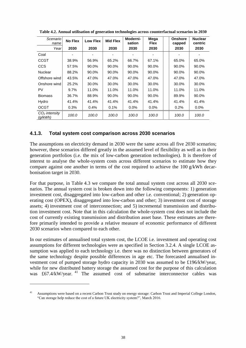
38
Table 4.2. Annual utilisation of generation technologies across counterfactual scenarios in 2030
Scenario name
No Flex Low Flex Mid Flex Moderni-
sation Mega Flex
Onshore capped
Nuclear centric
Year 2030 2030 2030 2030 2030 2030 2030
Coal - - - - - - -
CCGT 38.9% 56.9% 65.2% 66.7% 67.1% 65.0% 65.0%
CCS 57.5% 90.0% 90.0% 90.0% 90.0% 90.0% 90.0%
Nuclear 88.2% 90.0% 90.0% 90.0% 90.0% 90.0% 90.0%
Offshore wind 43.5% 47.0% 47.0% 47.0% 47.0% 47.0% 47.0%
Onshore wind 25.2% 30.0% 30.0% 30.0% 30.0% 30.0% 30.0%
PV 9.7% 11.0% 11.0% 11.0% 11.0% 11.0% 11.0%
Biomass 36.7% 88.9% 90.0% 90.0% 90.0% 89.9% 90.0%
Hydro 41.4% 41.4% 41.4% 41.4% 41.4% 41.4% 41.4%
OCGT 0.3% 0.4% 0.1% 0.0% 0.0% 0.2% 0.0%
CO2 intensity (g/kWh)
100.0 100.0 100.0 100.0 100.0
100.0 100.0
4.1.3. Total system cost comparison across 2030 scenarios
The assumptions on electricity demand in 2030 were the same across all five 2030 scenarios;
however, these scenarios differed greatly in the assumed level of flexibility as well as in their
generation portfolios (i.e. the mix of low-carbon generation technologies). It is therefore of
interest to analyse the whole-system costs across different scenarios to estimate how they
compare against one another in terms of the cost required to achieve the 100 g/kWh decar-
bonisation target in 2030.
For that purpose, in Table 4.3 we compare the total annual system cost across all 2030 sce-
narios. The annual system cost is broken down into the following components: 1) generation
investment cost, disaggregated into low-carbon and other i.e. conventional; 2) generation op-
erating cost (OPEX), disaggregated into low-carbon and other; 3) investment cost of storage
assets; 4) investment cost of interconnection; and 5) incremental transmission and distribu-
tion investment cost. Note that in this calculation the whole-system cost does not include the
cost of currently existing transmission and distribution asset base. These estimates are there-
fore primarily intended to provide a relative measure of economic performance of different
2030 scenarios when compared to each other.
In our estimates of annualised total system cost, the LCOE i.e. investment and operating cost
assumptions for different technologies were as specified in Section 3.2.4. A single LCOE as-
sumption was applied to each technology i.e. there was no distinction between generators of
the same technology despite possible differences in age etc. The forecasted annualised in-
vestment cost of pumped storage hydro capacity in 2030 was assumed to be £196/kW/year,
while for new distributed battery storage the assumed cost for the purpose of this calculation
was £67.4/kW/year.41
The assumed cost of submarine interconnector cables was
41 Assumptions were based on a recent Carbon Trust study on energy storage: Carbon Trust and Imperial College London,
“Can storage help reduce the cost of a future UK electricity system?”, March 2016.

39
£96/MW/km/year (the assumed lengths of different interconnection links was adjusted to take
into account the cost of substations and any onshore transmission grid reinforcements). Given
a number of uncertainties associated with estimating the cost of DSR deployment42
, this cost
is not included in the total annual cost calculation.43
For a similar reason, the cost estimate of
the Modernisation scenario does not include the cost of implementing the improvements in
system operation practices.
Table 4.3. Total annual system cost by component in counterfactual 2030 scenarios (in £m/year)
No Flex Low Flex Mid Flex Moderni-
sation Mega Flex
Onshore Capped
Nuclear Centric
Gen. CAPEX (low-C) 23,988 20,865 20,589 20,427 20,375 20,786 20,446
Gen. CAPEX (other) 4,329 3,445 2,919 2,919 2,457 2,919 2,539
OPEX (low-C) 1,873 2,442 2,448 2,443 2,439 2,449 3,034
OPEX (other) 4,189 4,142 4,124 4,121 4,115 4,127 4,038
Interconnection CAPEX 491 612 678 678 856 678 678
Transmission CAPEX 0 0 0 0 0 0 0
Distribution CAPEX 791 307 189 188 175 189 186
Storage CAPEX 691 1,028 1,364 1,364 1,701 1,364 1,364
Total 36,352 32,841 32,312 32,141 32,118 32,512 32,285
Savings vs. No Flex - 3,512 4,040 4,211 4,234 3,840 4,067
All 2030 systems include a significant amount of low-carbon generation capacity required to
meet the 100 g/kWh target. Given that low-carbon generation technologies tend to be charac-
terised by high investment cost and low operating cost, the investment cost of low-carbon
generation dominates the total system cost, accounting for about 60% of the total. At the
same time the generation CAPEX of conventional generators is 5-9 times lower. Operating
cost in all except the Low Flex scenario accounts for just over a fifth of total cost, and within
that category broadly a third is associated with the OPEX of low-carbon generators (mostly
nuclear, CCS and biomass as wind and PV have near-zero operating costs), while the rest is
the OPEX of conventional gas generation.
The storage CAPEX category is also significant given the relatively large assumed volume of
storage being available in the system (13.7 GW in total in the Mid Flex and 18.7 GW in the
Mega Flex scenario). Interconnection investment cost is also visible but does not exceed 2-
3% of the total system cost. In terms of transmission network investment, virtually no addi-
tional investment is required into the key GB transmission corridors.44
Finally, the incre-
mental investment in distribution grid for flexible scenarios (Mid Flex and above) is just be-
42 As an example of an attempt to estimate the cost of DSR while considering the uncertainty of its future evolution, see
e.g. Imperial College London, Carbon Trust, “An analysis of electricity system flexibility for Great Britain”, report for
DECC, October 2016.
43 It may be argued that because the enabling technology (smart meters) is mandated under all scenarios, and pricing DSR
is a complex task, it can be assumed that the cost of DSR is price-neutral across the scenarios i.e. that differences be-
tween scenarios provide a valid estimate of total system cost differentials.
44 Note that due to aggregated representation of GB transmission network used in the modelling, this would not capture
the cost of any local network reinforcements or replacements.

40
low the £200m mark. In scenarios with lower flexibility, however, the distribution CAPEX
increases considerably, almost doubling in the Low Flex scenario and more than quadrupling
in the No Flex scenario.
The total level of annualised system cost is also presented graphically in Figure 4.5 for all
2030 scenarios, as well as for the period 2015-2025. Total system cost between 2015 and
2025 is lower than in 2030 as the result of lower low-carbon generation capacity as well as
lower annual demand level.
Figure 4.5. Total annual system cost in counterfactual scenarios
Unsurprisingly, the overall system cost in 2030 is the highest in the Low Flex scenario, while
the enhancement of flexibility delivers savings of up to £4.2bn/year. Figure 4.6 further disag-
gregates the cost differentials between 2030 scenarios and the No Flex scenario into individ-
ual components.
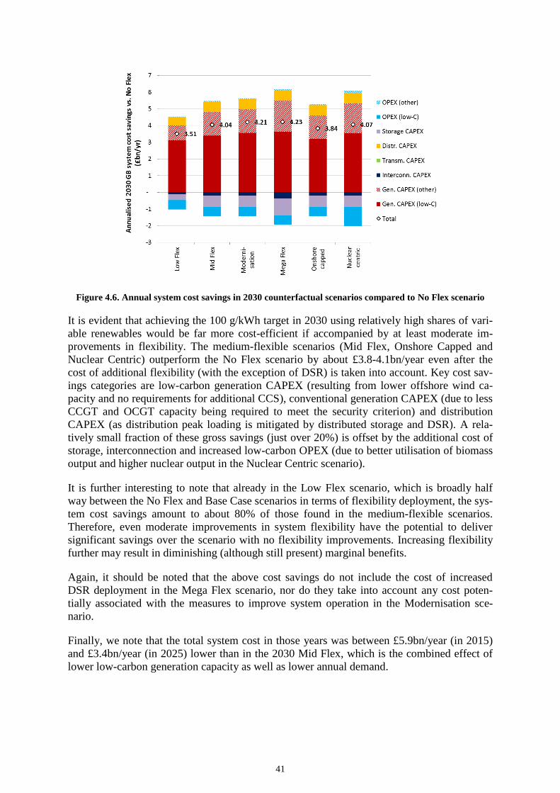
41
Figure 4.6. Annual system cost savings in 2030 counterfactual scenarios compared to No Flex scenario
It is evident that achieving the 100 g/kWh target in 2030 using relatively high shares of vari-
able renewables would be far more cost-efficient if accompanied by at least moderate im-
provements in flexibility. The medium-flexible scenarios (Mid Flex, Onshore Capped and
Nuclear Centric) outperform the No Flex scenario by about £3.8-4.1bn/year even after the
cost of additional flexibility (with the exception of DSR) is taken into account. Key cost sav-
ings categories are low-carbon generation CAPEX (resulting from lower offshore wind ca-
pacity and no requirements for additional CCS), conventional generation CAPEX (due to less
CCGT and OCGT capacity being required to meet the security criterion) and distribution
CAPEX (as distribution peak loading is mitigated by distributed storage and DSR). A rela-
tively small fraction of these gross savings (just over 20%) is offset by the additional cost of
storage, interconnection and increased low-carbon OPEX (due to better utilisation of biomass
output and higher nuclear output in the Nuclear Centric scenario).
It is further interesting to note that already in the Low Flex scenario, which is broadly half
way between the No Flex and Base Case scenarios in terms of flexibility deployment, the sys-
tem cost savings amount to about 80% of those found in the medium-flexible scenarios.
Therefore, even moderate improvements in system flexibility have the potential to deliver
significant savings over the scenario with no flexibility improvements. Increasing flexibility
further may result in diminishing (although still present) marginal benefits.
Again, it should be noted that the above cost savings do not include the cost of increased
DSR deployment in the Mega Flex scenario, nor do they take into account any cost poten-
tially associated with the measures to improve system operation in the Modernisation sce-
nario.
Finally, we note that the total system cost in those years was between £5.9bn/year (in 2015)
and £3.4bn/year (in 2025) lower than in the 2030 Mid Flex, which is the combined effect of
lower low-carbon generation capacity as well as lower annual demand.

42
4.2. Technology-specific integration costs
This section discusses the results of System Integration Cost studies based on the approach
laid out in Section 3.6.2. All SIC studies are based on a marginal addition of LCGT capacity
accompanied with a marginal removal of nuclear capacity. To ensure a like-for-like replace-
ment, the nominal annually available output of added LCGT and removed nuclear capacity is
kept equal. Following the replacement of nuclear with another LCGT the system is allowed
to readjust itself by finding a new set of optimal decisions on system operation and on in-
vestment in selected generation technologies.
The SIC of a given LCGT is evaluated by dividing the change in total system cost with the
volume of replaced low-carbon output. The unique feature of our whole-system modelling
approach allows for a component-by-component disaggregation of the cost differential, ena-
bling the identification of which sectors and technologies are the key contributors to changes
in investment and operation cost.
4.2.1. Offshore wind
The results of the SIC studies for offshore wind are shown in Figure 4.7 for the Base Case
scenarios between 2015 and 203045
, and in Figure 4.8 for all 2030 scenarios. For each sce-
nario the SIC is broken down into components, which refer to operating cost (OPEX), gen-
eration investment (G CAPEX) and transmission and distribution network investment (T
CAPEX and D CAPEX). OPEX and G CAPEX categories are further subdivided according
to different generation technologies where change in operating and investment cost is ob-
served in the SIC study compared to the counterfactual scenario.
Figure 4.7. SIC of offshore wind compared to nuclear in Base Case scenarios between 2015 and 2030
45 The Mid Flex scenario is used in this and subsequent sections to make comparisons between 2030 and earlier years.

43
Figure 4.8. SIC of offshore wind compared to nuclear across different 2030 scenarios
Both figures show that in each scenario the replacement of nuclear with wind capacity has a
positive (net) G CAPEX component, which is predominantly a result of investing in addi-
tional OCGT and CCGT capacity. The requirement to firm up added wind with conventional
capacity results from the low capacity value (i.e. low derating factor) of wind in terms of con-
tributing to secure capacity margin in the system. In the 2030 scenarios it is also possible to
observe a component “G CAPEX – diff.” in the SIC; this component refers to the extra ca-
pacity of an LCGT (offshore wind in this case) that had to be added in excess of the energy-
equivalent capacity in order to meet the 100 g/kWh emission target.46
Replacement of nuclear with offshore wind also triggers changes in operating cost of thermal
generators in varying proportions, driven by the additional requirements for ancillary services
(reserve and response) arising from increased wind capacity, as well as the seasonality of off-
shore wind output profile, which tends to be higher over winter and autumn months than dur-
ing summer, making it better aligned with the seasonal variations in system demand than the
largely flat output profile of nuclear generators. The exact change in operating cost is the re-
sult of the composition of thermal generation mix assumed to exist in a given scenario, as
well as the combination of gas, coal and carbon prices across time.
It is further interesting to note that while the SIC of offshore wind increases between 2020
and 2025, the integration cost in 2030 is lower than in 2025. This reduction in SIC is primar-
ily driven by significant improvements in flexibility between 2025 and 2030 assumed in the
scenarios (see Section 3.4.1 for detailed assumptions on flexibility). Nevertheless, as demon-
strated in Figure 4.8, in the No Flex scenario the SIC would be significantly higher, around
£48/MWh, indicating a very low ability of the system to cost-effectively integrate RES gen-
eration.
46 This is in line with the method chosen to quantify System Integration Cost, see Section 2.3.

44
Another point to note is that in 2030 scenarios with higher flexibility (e.g. in Base Case in
Figure 4.7) there is a noticeable component of SIC associated with distribution network in-
vestment (D CAPEX), which may appear counterintuitive at first given that new offshore
wind sites would obviously connect at transmission level. The reason for this effect is the
whole-system approach to system optimisation: the distributed storage resource, assumed to
exist in significant volumes in all 2030 scenarios, now shifts the utilisation of its flexibility
slightly away from minimising distribution network loading (and the associated investment
cost savings) towards supporting the management of added wind resource. The ability to cap-
ture such trade-offs represents a unique feature of our modelling approach and the WeSIM
model.
To get a measure of how the whole-system costs of nuclear and offshore wind compare when
their investment and operation cost is taken into account, it is beneficial to compare differ-
ences in LCOE against the SIC obtained through running the model for various scenarios.
According to the LCOE assumptions in Section 3.2.4, the cost of offshore wind is projected
to drop over time, while the cost of nuclear would remain relatively stable (with some reduc-
tion envisaged in the Nuclear Centric scenario). Given that the analysis shows that SIC of
offshore wind also varies across scenarios, the relationship between the whole-system cost of
nuclear and offshore wind will also change as function of the scenario.
Table 4.4 and Table 4.5 summarise the projected LCOE evolution for nuclear and offshore
wind and contrast the LCOE differentials to the relative SIC of offshore wind quantified
across different scenarios.
Table 4.4. LCOE differentials between offshore wind and nuclear compared to SIC in Base Case between
2015 and 2030 (in £/MWh)
Scenario name Basecase 15 Basecase 20 Basecase 25 Mid Flex
Year 2015 2020 2025 2030
LCOE
Nuclear 93 93 90 90
Offshore 133 106 80 75
Difference -40 -13 10 15
SIC
Offshore vs. nuclear
9.7 10.1 11.0 7.8
Table 4.5. LCOE differentials between offshore wind and nuclear compared to SIC across 2030 scenarios
(in £/MWh)
Scenario name No Flex Low Flex Mid Flex Moderni-
sation Mega Flex
Onshore capped
Nuclear centric
LCOE
Nuclear 90 90 90 90 90 90 80
Offshore 75 75 75 75 75 70 80
Difference 15 15 15 15 15 20 0
SIC
Offshore vs. nuclear
48.4 11.2 7.8 5.5 5.5 8.1 7.5

45
From Table 4.4 we observe that between 2015 and 2025 the SIC of offshore wind is higher
than its cost advantage (if any) over nuclear, and this is indicated by red cell shading. In the
2030 Mid Flex scenario, however, both SIC and LCOE of offshore wind reduce sufficiently
to make its whole-system cost lower than that of nuclear (indicated by green cell colour). Ta-
ble 4.5 shows that with the exception of No Flex and Nuclear Capped scenarios, in all other
scenarios the SIC of offshore wind is lower than its cost advantage over nuclear, resulting in
a lower whole-system cost of wind.
4.2.2. Onshore wind
The results of the SIC studies for onshore wind are shown in Figure 4.9 for the Base Case
between 2015 and 2030, and in Figure 4.10 for all 2030 scenarios.
Figure 4.9. SIC of onshore wind compared to nuclear in Base Case scenario between 2015 and 2030

46
Figure 4.10. SIC of onshore wind compared to nuclear across 2030 scenarios
The magnitude of SIC before 2030 is very similar as for offshore wind. In 2030 we again ob-
serve a very high SIC in the No Flex scenario, driven by high RES output curtailment. Sce-
narios with lower onshore capacity (Onshore Capped and Nuclear Centric) result in a slightly
lower SIC than for offshore wind, while on the other hand the SIC in Modernisation and
Mega Flex scenarios is slightly higher than for offshore wind. Nevertheless, generally speak-
ing there are no great differences between the SIC of onshore and offshore wind.
Table 4.6 and Table 4.7 compare the assumed LCOE cost differentials of onshore wind and
nuclear with the SIC results in order to establish in which scenarios is the whole-system cost
of onshore wind lower than that of nuclear. Given that the assumed LCOE of onshore wind is
considerably lower than the cost of nuclear (by up to £30/MWh), the whole-system cost of
onshore wind is more competitive than nuclear in almost every scenario considered, with the
exception of the extreme No Flex scenario in 2030, where the SIC of onshore wind takes a
very high value.
Table 4.6. LCOE differentials between onshore wind and nuclear compared to SIC in Base Case between
2015 and 2030 (in £/MWh)
Scenario name Basecase 15 Basecase 20 Basecase 25 Mid Flex
Year 2015 2020 2025 2030
LCOE
Nuclear 93 93 90 90
Onshore 75 65 60 60
Difference 18 28 30 30
SIC
Onshore vs. nuclear
9.9 10.2 11.9 7.5

47
Table 4.7. LCOE differentials between onshore wind and nuclear compared to SIC across 2030 scenarios
(in £/MWh)
Scenario name No Flex Low Flex Mid Flex Moderni-
sation Mega Flex
Onshore capped
Nuclear centric
LCOE
Nuclear 90 90 90 90 90 90 80
Onshore 60 60 60 60 60 60 60
Difference 30 30 30 30 30 30 20
SIC
Onshore vs. nuclear
40.2 10.2 7.5 7.3 7.2 7.2 7.1
4.2.3. Solar PV
The SIC of solar PV is given in Figure 4.11 for the Base Case scenario between 2015 and
2030, and in Figure 4.12 for all 2030 scenarios.
While the SIC in 2015, 2020 and 2025 is very similar as for onshore and offshore wind, in
2030 the integration cost is considerably higher than the SIC of wind. This is particularly re-
flected in the higher distribution CAPEX component across all 2030 scenarios. High distribu-
tion investment arises as the result of increased reversed flows in distribution networks,
which require reinforcement of the grid. There is also a noticeable component of additional
PV investment to maintain emissions (G CAPEX – diff.), as the seasonality of PV generation
is exactly the opposite of system demand: high PV output in summer coincides with low sys-
tem demand and vice versa. Hence, the generation displaced by PV is likely to be less car-
bon-intensive than average, meaning that carbon benefits of additional PV would be lower
than those of removed nuclear output and consequently more PV capacity would be needed to
maintain the 100 g/kWh intensity. Note also that the PV capacity is not assumed to be uni-
formly dispersed across GB; a much higher installation density is foreseen in the south of the
country.
Figure 4.11. SIC of solar PV compared to nuclear in Base Case scenario between 2015 and 2030

48
Figure 4.12. SIC of solar PV compared to nuclear across 2030 scenarios
As with offshore and onshore wind, the SIC in the No Flex scenario is found to be very high,
above £40/MWh. This is again the consequence of high curtailment: about 25% of the PV
output added in the SIC study is curtailed. The system establishes the same CO2 intensity by
replacing a significant volume of OCGT with CCGT capacity.
The enhanced flexibility i.e. additional storage and DSR in the Mega Flex scenario manage to
almost completely eliminate the SIC component associated with distribution investment cost.
In general, however, the SIC of PV tends to be higher in 2030 than for both onshore and off-
shore wind. On the other hand, because the assumed LCOE of solar PV in 2030 was rela-
tively low (£15/MWh lower than nuclear in Nuclear Centric and £25/MWh in all other sce-
narios), in all scenarios except No Flex solar PV is competitive with nuclear when its whole-
system cost is considered.
Table 4.8 and Table 4.9 compare the LCOE assumptions for solar PV and nuclear with the
numerical results for SIC of solar PV generation. The tables suggest that from 2025 onwards
the whole-system cost of solar PV becomes more competitive than that of nuclear, or in other
words that its cost advantage over nuclear exceeds its SIC. The only exception to this is again
the No Flex scenario, where the SIC of solar PV (similar to offshore and onshore wind) has a
value of over £40/MWh.

49
Table 4.8. LCOE differentials between solar PV and nuclear compared to SIC in Base Case between 2015
and 2030 (in £/MWh)
Scenario name Basecase 15 Basecase 20 Basecase 25 Mid Flex
Year 2015 2020 2025 2030
LCOE
Nuclear 93 93 90 90
Solar PV 101 86 75 65
Difference -8 7 15 25
SIC
Solar PV vs. nuclear
9.5 9.6 11.2 14.4
Table 4.9. LCOE differentials between solar PV and nuclear compared to SIC across 2030 scenarios (in
£/MWh)
Scenario name No Flex Low Flex Mid Flex Moderni-
sation Mega Flex
Onshore capped
Nuclear centric
LCOE
Nuclear 90 90 90 90 90 90 80
Solar PV 65 65 65 65 65 65 65
Difference 25 25 25 25 25 25 15
SIC
Solar PV vs. nuclear
43.5 17.4 14.4 11.8 8.1 13.6 12.3
4.2.4. Biomass
Finally, the SIC of biomass generation is depicted in Figure 4.13 for the Base Case studies
between 2015 and 2030, and in Figure 4.14 for all 2030 scenarios. Given that biomass repre-
sents a flexible form of renewable generation, and unlike wind and PV does not increase the
volume of required ancillary services, its integration costs are correspondingly lower, and in
some scenarios even become negative. In the majority of scenarios the absolute magnitude of
SIC of biomass is rather low, with the results being in the range ±£2/MWh. In the No Flex
scenario the SIC of biomass drops to -£7/MWh, as the operation of biomass plant is expected
to be more flexible than nuclear.

50
Figure 4.13. SIC of biomass compared to nuclear Base Case scenario between 2015 and 2030
Figure 4.14. SIC of biomass compared to nuclear across 2030 scenarios
Low SIC of biomass indicates that its whole-system benefits are similar to those of nuclear,
so the comparison between the whole-system costs of the two technologies provides a very
similar outcome to the comparison of their LCOEs. Table 4.10 and Table 4.11 compare the
LCOEs of nuclear and biomass with the SIC results presented above. Despite very low, or
sometimes even negative SIC of biomass, its higher LCOE assumption than nuclear results in
a whole-system cost of biomass that is higher than that of nuclear in all scenarios and in all
years.

51
Table 4.10. LCOE differentials between biomass and nuclear compared to SIC in Base Case between
2015 and 2030 (in £/MWh)
Scenario name Basecase 15 Basecase 20 Basecase 25 Mid Flex
Year 2015 2020 2025 2030
LCOE
Nuclear 93 93 90 90
Biomass 108 108 108 108
Difference -15 -15 -18 -18
SIC
Biomass vs. nuclear
0.9 1.1 -0.4 -1.3
Table 4.11. LCOE differentials between biomass and nuclear compared to SIC across 2030 scenarios (in
£/MWh)
Scenario name No Flex Low Flex Mid Flex Moderni-
sation Mega Flex
Onshore capped
Nuclear centric
LCOE
Nuclear 90 90 90 90 90 90 80
Biomass 108 108 108 108 108 108 108
Difference -18 -18 -18 -18 -18 -18 -28
SIC
Biomass vs. nuclear
-6.9 0.6 -1.3 0.0 -0.6 -0.8 -0.1

52
5. Illustration of key aspects of hourly system operation
In this chapter we provide several examples of hourly system operation for selected situations
that are typical for the system. The examples presented are taken from the Mid Flex scenario
for 2030.
5.1. Impact of flexible options on residual demand
One of the key advantages of flexible options, in particular energy storage, DSR and inter-
connectors, is the ability to modify the residual demand profile seen by the generators in the
system. A flatter demand profile requires lower use of high-cost peaking plants, while at the
same time maximising the utilisation of baseload plant characterised by low marginal costs.
For the example of the Mid Flex scenario in 2030, Figure 5.1 shows how the original load
duration curve (LDC) is modified by the model through optimised use of three flexible op-
tions (storage, DSR and interconnection).
The original demand profile in 2030 (before and DSR actions) had a peak of 71.3 GW, corre-
sponding to the highest value on the ‘Original demand’ curve in Figure 5.1. The way WeSIM
ensures sufficient capacity margin is to build the required firm capacity so that the Loss of
Load Expectation (LOLE) parameter does not exceed 3 hours per year. In practice, for a
thermal system without any DSR or storage, this results in the capacity margin of approxi-
mately 20% over the system peak.
In the No Flex scenario (see Section 3.6.1) the model adds 41.7 GW of flexible peaking
(OCGT) capacity. When this is added to the volume of other firm capacity (CCGT, CCS, nu-
clear, biomass, hydro and storage), the total firm capacity in the system totals about 86 GW,
or around 20% above the peak demand of 71.3 GW. In the Mid Flex scenario on the other
hand, the combined effect of DSR, additional storage and interconnection is that only about
20 GW of flexible peaking capacity is required in the system to maintain the same level of
security of supply, i.e. to keep the LOLE at 3 hours per year.

53
Figure 5.1. Synchronised load duration curves for system demand before and after optimising the use of
DSR, energy storage and interconnection
The curves shown in Figure 5.1 are synchronised in the sense that once the LDC of the origi-
nal demand is constructed, each corresponding data point plotted on the modified demand
curve occurred at the same time as the original demand point with a given time coordinate.
As expected, the shape of the demand curve changes to improve efficiency of electricity gen-
eration: high peaks in the original demand curve are reduced, while the low-demand periods
see an increase in demand.
The same demand curves are plotted again in Figure 5.2 without retaining the synchronicity,
i.e. by simply ordering the modified demand curve points in descending order. As expected,
the shape of the LDC becomes flatter with additional flexibility. It is nevertheless interesting
to note that after applying all three flexible options the peak demand ends up being slightly
higher than after applying just DSR. This is because the system optimises the use of flexibil-
ity to minimise system cost, so the resulting demand profile is also adapting to fluctuations in
the output of variable RES technologies (wind and solar). The new peak in modified demand

54
(occurring at a different point in time than the original peak) is likely to coincide with periods
of high renewable output.
Figure 5.2. Non-synchronised LDCs for system demand before and after optimising the use of DSR, en-
ergy storage and interconnection
To illustrate the effect of flexibility on net demand LDC, Figure 5.3 shows the LDC for net
demand before and after applying flexible options. It is evident that without flexibility the net
demand would occasionally become negative, necessitating RES output curtailment. In the
presence of flexible options however, the modified net demand curve is maintained well
above zero and is much more evenly balanced between periods of low and high net demand.
Figure 5.3. Synchronised net demand LDCs before and after optimising the use of flexible options
It is interesting to observe that for most of the year the modified net demand profile is capped
at about 30 GW, which is only exceeded during a small number of hours (ca. 50) coinciding
with peak demand hours. This occurs because the model is trying to maximise the utilisation

55
of firm capacity represented by nuclear, CCS, biomass, hydro and CCGT generation (total-
ling around 30 GW). On infrequent occasions when the 30 GW of generation output has to be
exceeded due to very high original demand, the model utilises high marginal cost OCGT
generators that are otherwise providing backup.
The role of flexibility in ensuring a more efficient operation of generation resources is even
more evident from Figure 5.4, which represents non-synchronised net demand LDCs. De-
ployment of DSR, storage and interconnection enables the peak net demand value seen by
conventional generators to drop from 62.3 GW to just 33.9 GW. On the other end of the spec-
trum, the minimum value of net demand increases from -8.6 GW (i.e. from a situation with an
excess RES output potentially necessitating curtailment) to 7.1 GW. The 30 GW threshold is
easily discernible from the post-flexibility net demand LDC, suggesting that in this scenario
(i.e. with the relevant assumptions made on demand, low-carbon and conventional generation
capacities and flexible options deployment) not more than 30 GW of mid-merit (i.e. non-
peaking) plant is required to cover the demand in all but a small number of peak demand
hours.
Figure 5.4. Non-synchronised net demand LDCs before and after optimising the use of flexible options
In order to further clarify the role of flexible peaking capacity, we note that the maximum
utilisation of non-renewable generation in 2030 (according to the green curve in Figure 5.4)
is 33.9 GW, or when deducting CCGT, CCS, nuclear, hydro and biomass output, this implies
the maximum utilisation of OCGT generation capacity at the level of 4.4 GW. This is consid-
erably lower than the 21.8 GW installed by the model, so one might question the need to in-
stall a seemingly excessive amount of peaking plant. However, the system operation simu-
lated in WeSIM is deterministic, and does not explicitly include the simulation of plant out-
ages. This is why WeSIM (as documented in detail in the Appendix) uses a separate set of
constraints to ensure that sufficient generation capacity margin is maintained to guarantee the
ability of the system to supply demand in all but 3 hours per year (on average). The model
therefore adds peaking capacity that would mostly not be used with a perfect (deterministic)
forecast, but is on the other hand crucial to ensure the ability of the system to cope with prob-
able outages of generating units at the assumed level of LOLE of 3 hours.

56
Increasing the allowed level of LOLE would inevitably result in a lower level of required ca-
pacity margin, reducing the need to add peaking capacity to the system.47
Nevertheless, the
impact on the level of SIC associated with VRES technologies, being the key focus of this
study, is unlikely to change materially as the result of relaxed security of supply criterion.
5.2. Winter vs. summer system operation
In Figure 5.5 we illustrate how the system operates on an hourly basis for a winter week in
January (results are from the 2030 Mid Flex scenario). The chart shows the hourly output of
all generation technologies as well as the utilisation of storage, net interconnection flows and
the impact of DSR on residual demand profile.
Figure 5.5. Hourly system dispatch for a winter week in 2030 (Mid Flex)
During the week depicted in the chart, wind output during the second day drops to a very low
level (with about 2.5 GW being the lowest output during that day). The system responds to
the combination of low RES output and high demand by maximising the imports via inter-
connectors as well as discharging energy storage during key hours of that day. As this is still
insufficient to meet the demand, the model also utilises some OCGT capacity to provide elec-
tricity during Day 2. One can also note that when wind output increases again starting from
Day 3, the model starts exporting electricity to neighbouring systems, while also taking the
opportunity to recharge energy storage.
During a typical summer week, depicted in Figure 5.6, the system is faced with much lower
demand requirements, while the output of variable RES generators (including solar PV that
provides peak output during summer) can be substantial. The model therefore minimises the
47 A very rough calculation shows that if LOLE was increased from 3 to 6 hours per year, the system in 2030 would need
about 4 GW less peaking capacity.
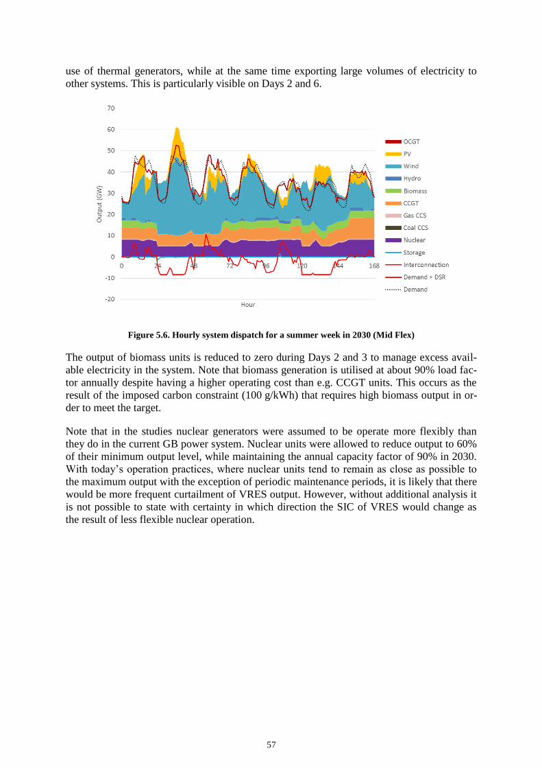
57
use of thermal generators, while at the same time exporting large volumes of electricity to
other systems. This is particularly visible on Days 2 and 6.
Figure 5.6. Hourly system dispatch for a summer week in 2030 (Mid Flex)
The output of biomass units is reduced to zero during Days 2 and 3 to manage excess avail-
able electricity in the system. Note that biomass generation is utilised at about 90% load fac-
tor annually despite having a higher operating cost than e.g. CCGT units. This occurs as the
result of the imposed carbon constraint (100 g/kWh) that requires high biomass output in or-
der to meet the target.
Note that in the studies nuclear generators were assumed to be operate more flexibly than
they do in the current GB power system. Nuclear units were allowed to reduce output to 60%
of their minimum output level, while maintaining the annual capacity factor of 90% in 2030.
With today’s operation practices, where nuclear units tend to remain as close as possible to
the maximum output with the exception of periodic maintenance periods, it is likely that there
would be more frequent curtailment of VRES output. However, without additional analysis it
is not possible to state with certainty in which direction the SIC of VRES would change as
the result of less flexible nuclear operation.

58
6. Sensitivity analysis
This chapter summarises the results of sensitivity analyses where a number of core assump-
tions have been modified to investigate the impact of these variations on system integration
cost of renewable generation.
6.1. Impact of retiring biomass before 2030
Biomass generation, in particular when associated with conversion of existing coal-fired
plants, is currently seen as a viable option for decarbonising the UK electricity supply in the
medium term. Nevertheless, there are concerns around the sustainability of biomass
sources.48
It is therefore of interest to assess the impact on SIC of renewable technologies of
the assumption that instead of 3.4 GW of biomass capacity assumed across all 2030 scenarios,
there would not be any biomass generators in operation in 2030.
As shown in Table 4.2, the utilisation of biomass in all 2030 scenarios except No Flex is very
close to the maximum (90%), despite a relatively high operating cost (around £70/MWh).
This follows from the 100 g/kWh carbon target imposed in 2030 scenarios and the fact that
biomass output was assumed to be zero-carbon, so the model maximised its utilisation. Given
that the 2030 scenarios were optimised for offshore wind capacity, it was more cost-efficient
to remove a unit of offshore wind capacity than to reduce the utilisation of biomass, despite
its variable cost being higher than e.g. the cost of CCGT.
Because of the setup of the scenarios, where a cost-optimal volume of offshore wind is cho-
sen to meet the 100 g/kWh target, reduction of low-carbon output from biomass will require
more offshore wind in the system to maintain the same level of carbon emissions. With eve-
rything else kept equal, one would expect that SIC of e.g. offshore wind would increase if the
volume of offshore wind in the scenario increases at the expense of biomass generation.
In the first step the model was run to establish the counterfactual cases for the five 2030 sce-
narios, in particular to determine the optimal volumes of offshore wind capacity that can be
removed from the system while maintaining the 100 g/kWh carbon intensity, similar to the
counterfactual scenario construction described in Section 3.6.1. Table 6.1 specifies the opti-
mised volumes of generation technologies and interconnection across the five 2030 scenarios
without biomass (this table is equivalent to Table 3.8, which specified optimal volumes for
the core scenarios).
48 For a more detailed discussion of the issue see e.g. DECC’s report “Life Cycle Impacts of Biomass Electricity in 2020”
(July 2014), the U.S. Natural Resources Defense Council’s issue brief “Think Wood Pellets are Green? Think Again”
(May 2015), or the Greenpeace report “Fuelling a BioMess: Why Burning Trees for Energy Will Harm People, the
Climate and Forests” (October 2011), providing a view from the Canadian perspective.

59
Table 6.1. Optimised capacities of technologies in 2030 counterfactual scenarios without biomass (in GW)
Technology Scenario
Mid Flex Onshore capped Nuclear centric Modernisation Mega Flex
OCGT 33.6 33.6 25.5 33.6 23.9
New CCGT* - - - 0.1 0.1
Offshore wind 29.0 36.7 18.0 28.3 28.1
Reduced wind** -2.0 -2.3 -3.0 -2.7 -2.9
New interconnection - - - - -
Notes: * CCGT capacity added on top of the capacity in Table 3.1. ** Reduction compared to the initial capacity in Table 3.1.
By comparing Table 6.1 with Table 3.8, it is evident that much less offshore wind has been
removed from the starting generation mixes, which is expected given the requirement to
maintain carbon emissions following the removal of biomass from the generation portfolio.
Instead of 8.8-9.6 GW of offshore wind that could be removed in the core scenarios, the ab-
sence of biomass in the 2030 mix allowed only 2 to 3 GW of offshore wind to be removed
from the starting generation mixes for the same emission intensity level. The absence of bio-
mass is also reflected in the increased volume of peaking OCGT capacity, added by the
model to maintain the same level of firm capacity i.e. to ensure sufficient capacity margin in
the system.
The quantitative results for SIC across the 2030 scenarios without biomass are shown in Fig-
ure 6.1 for the four analysed renewable technologies.
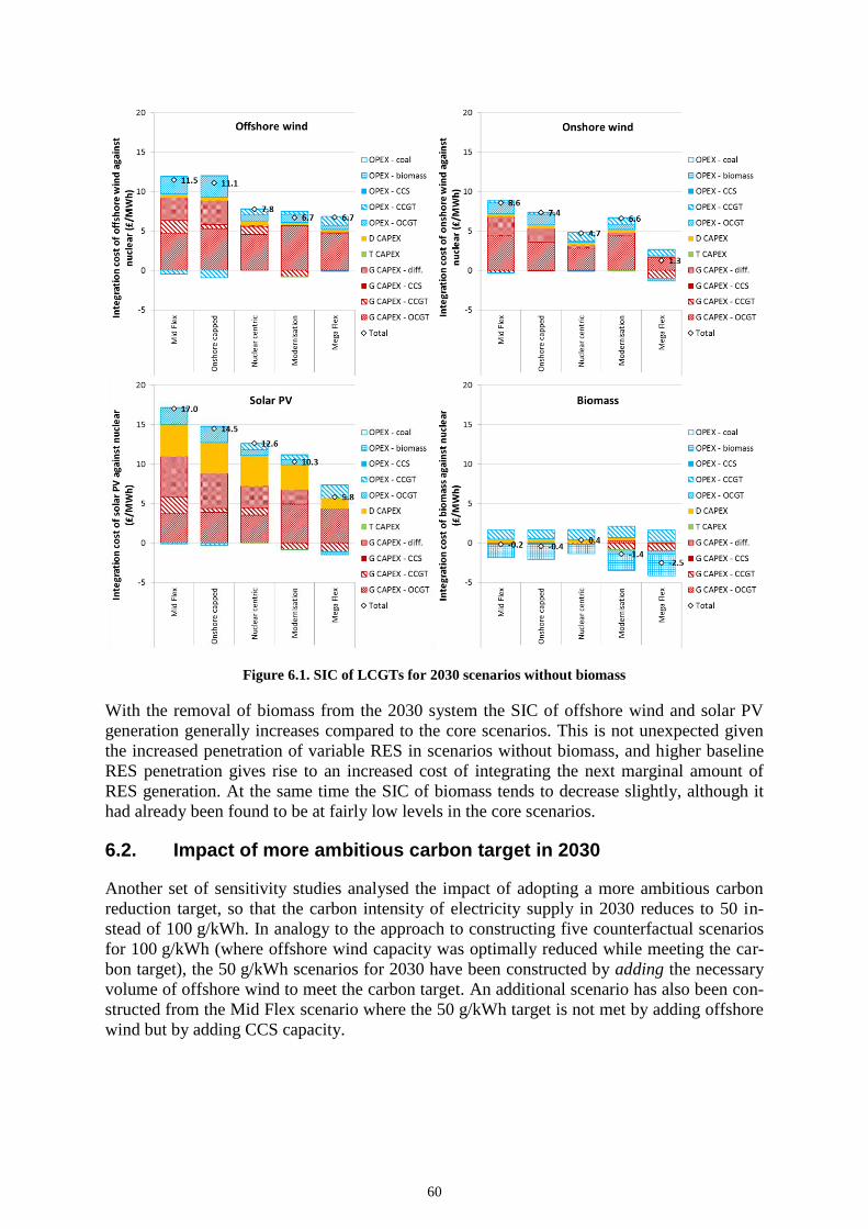
60
Figure 6.1. SIC of LCGTs for 2030 scenarios without biomass
With the removal of biomass from the 2030 system the SIC of offshore wind and solar PV
generation generally increases compared to the core scenarios. This is not unexpected given
the increased penetration of variable RES in scenarios without biomass, and higher baseline
RES penetration gives rise to an increased cost of integrating the next marginal amount of
RES generation. At the same time the SIC of biomass tends to decrease slightly, although it
had already been found to be at fairly low levels in the core scenarios.
6.2. Impact of more ambitious carbon target in 2030
Another set of sensitivity studies analysed the impact of adopting a more ambitious carbon
reduction target, so that the carbon intensity of electricity supply in 2030 reduces to 50 in-
stead of 100 g/kWh. In analogy to the approach to constructing five counterfactual scenarios
for 100 g/kWh (where offshore wind capacity was optimally reduced while meeting the car-
bon target), the 50 g/kWh scenarios for 2030 have been constructed by adding the necessary
volume of offshore wind to meet the carbon target. An additional scenario has also been con-
structed from the Mid Flex scenario where the 50 g/kWh target is not met by adding offshore
wind but by adding CCS capacity.

61
Table 6.2 summarises the key capacity additions in the five 2030 scenarios necessary to reach
the 50 g/kWh carbon intensity. The table suggest that in Nuclear Centric, Modernisation and
Mega Flex scenarios, which are characterised by either very high flexibility or moderate wind
deployment levels, only about 2.2-2.5 GW of additional offshore wind capacity would be
necessary to meet the 50 g/kWh target. In the two scenarios with high wind capacity and me-
dium flexibility level, Mid Flex and Onshore Capped, it is necessary to install 3.2-3.6 GW of
additional offshore wind to comply with the 50 g/kWh limit, but it also becomes necessary to
install additional interconnection capacity between GB and mainland Europe, in the amount
of 5-6 GW.
Table 6.2. Optimised capacities in 2030 counterfactual scenarios when meeting 50 g/kWh target (in GW)
Technology
Scenario
Mid Flex Onshore capped
Nuclear centric
Modernisa-tion
Mega Flex Mid Flex
(CCS)
OCGT 30.1 30.0 21.9 30.0 20.2 28.1
New CCGT* - 0.1 - - 0.1 -
Added wind** 3.6 3.2 2.2 2.4 2.4 -
Added CCS** - - - - - 1.9
New interconnec-tion***
5.1 6.1 - - - -
Notes: * CCGT capacity added on top of the capacity in Table 3.1. ** Compared to the initial capacity in Table 3.1. *** Compared to the deployment level in Table 3.6.
The results of SIC studies for the 50 g/kWh scenarios are shown in Figure 6.2 for offshore
and onshore wind and PV. An immediate observation is that in Mid Flex and Onshore
Capped scenarios the SIC of both wind and PV becomes dramatically higher, about 2-3 times
higher than the SIC found in 100 g/kWh scenarios. In these two scenarios the SIC of wind
and PV is dominated by the excess wind or PV capacity added on top of the energy equiva-
lent amount to keep the system emissions constant.
As an illustration, in the Mid Flex scenario, instead of replacing 1 GW of nuclear with the
energy-equivalent 1.9 GW of offshore wind, the model in fact adds 3.4 GW i.e. almost dou-
ble the equivalent amount. This occurs because the integration of wind and PV generation in
those scenarios becomes challenging in the context of retaining the same carbon intensity: the
addition of e.g. wind in SIC studies displaces a significant amount of low-carbon output of
biomass49
, which requires additional wind capacity to be added in order to maintain system
carbon emissions. Only with 3.4 GW of additional offshore wind capacity does the model
manage to balance the system with 50 g/kWh carbon intensity. This inability to efficiently
integrate VRES generation also indicates that purely increasing wind capacity beyond about
50 GW with the level of flexibility assumed in the Mid Flex scenario may not be the best
49 Displacement of biomass output is observed despite the reduction of nuclear capacity by 1 GW. The reason for this is
that the added wind capacity that is energy-equivalent to 1 GW of nuclear produces the same output on average; how-
ever the wind output fluctuates so that when it is higher than 1 GW it would displace biomass despite there being 1 GW
less of nuclear generation. When wind output is lower than the average on the other hand, the missing energy cannot be
provided by increased biomass output as biomass will be constrained by its installed capacity.
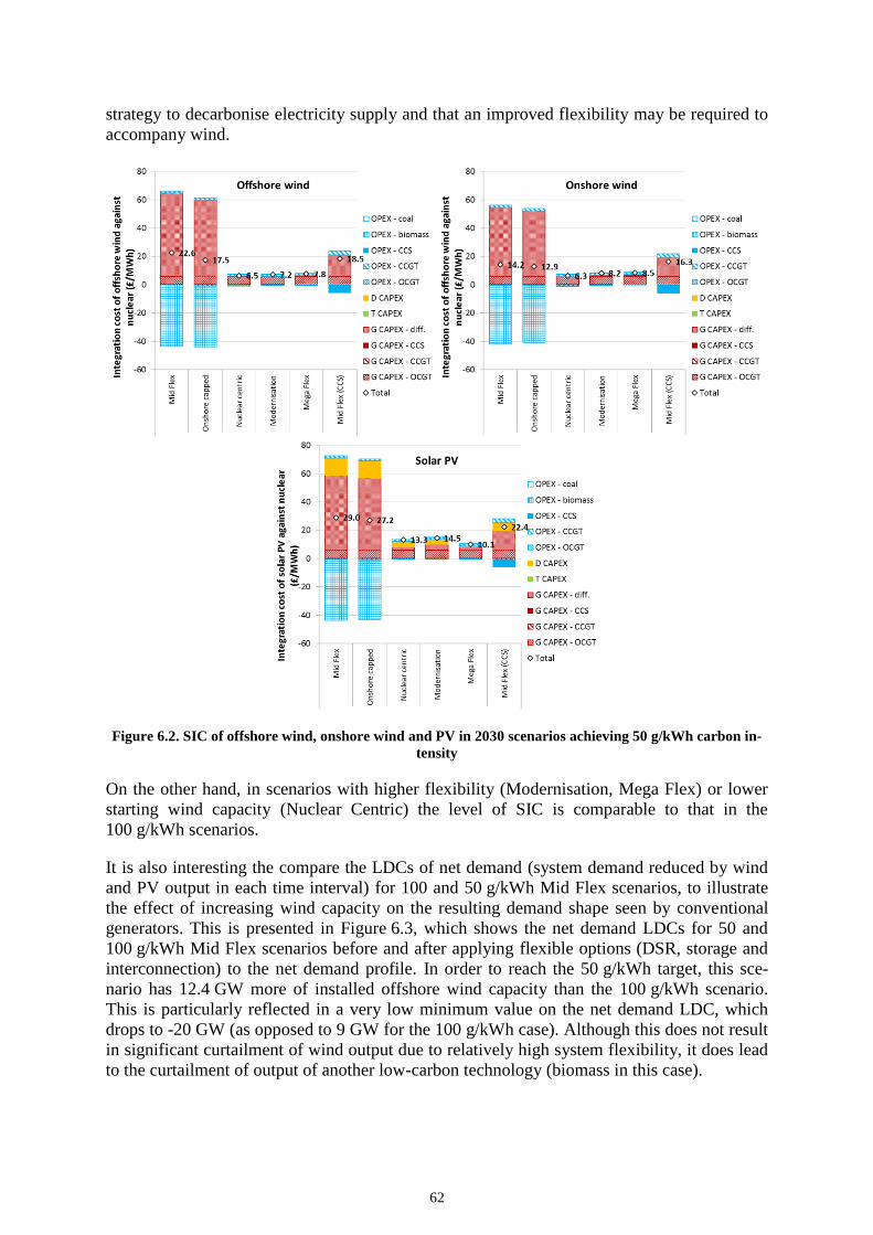
62
strategy to decarbonise electricity supply and that an improved flexibility may be required to
accompany wind.
Figure 6.2. SIC of offshore wind, onshore wind and PV in 2030 scenarios achieving 50 g/kWh carbon in-
tensity
On the other hand, in scenarios with higher flexibility (Modernisation, Mega Flex) or lower
starting wind capacity (Nuclear Centric) the level of SIC is comparable to that in the
100 g/kWh scenarios.
It is also interesting the compare the LDCs of net demand (system demand reduced by wind
and PV output in each time interval) for 100 and 50 g/kWh Mid Flex scenarios, to illustrate
the effect of increasing wind capacity on the resulting demand shape seen by conventional
generators. This is presented in Figure 6.3, which shows the net demand LDCs for 50 and
100 g/kWh Mid Flex scenarios before and after applying flexible options (DSR, storage and
interconnection) to the net demand profile. In order to reach the 50 g/kWh target, this sce-
nario has 12.4 GW more of installed offshore wind capacity than the 100 g/kWh scenario.
This is particularly reflected in a very low minimum value on the net demand LDC, which
drops to -20 GW (as opposed to 9 GW for the 100 g/kWh case). Although this does not result
in significant curtailment of wind output due to relatively high system flexibility, it does lead
to the curtailment of output of another low-carbon technology (biomass in this case).

63
Figure 6.3. Non-synchronised net demand LDCs in 100 and 50 g/kWh Mid Flex runs before and after
applying flexible options
Finally, in the Mid Flex scenario with CCS optimally added rather than offshore wind, the
SIC of wind and PV becomes similar to the levels observed in Mid Flex and Onshore Capped
scenarios. In the case of PV the SIC in this scenario is actually lower than the integration cost
in Mid Flex scenario with 50 g/kWh target imposed by installing additional wind capacity.
An implication of this is that there may be merit in considering a certain amount of CCS as
part of the low-carbon generation mix thus ensuring flexibility on the generation side.
6.3. Impact of system flexibility
Our previous studies, such as the recent CCC study, demonstrated the critical role of flexible
options such as energy storage and DSR in cost-effective integration of variable renewables.
A high level of flexibility in the system may help to manage the integration cost and keep it at
an acceptable level. Although varying flexibility was a prominent feature of the analysed sce-
narios, given the pivotal role of flexibility in supporting cost-effectiveness of VRES integra-
tion, an additional set of sensitivity studies was run to evaluate the impact of varying flexibil-
ity across the scenarios adopted in this study on SIC of VRES.
Table 6.3 details the variations in flexibility assumptions around the central values assumed
in baseline scenarios. Two further flexibility levels have been considered in 2020 and 2025,
Low and High. In 2030, in addition to the Mid Flex and Mega Flex scenarios, two lower
flexibility levels were analysed (as already defined previously in Section 3.1):
Low Flex: same starting generation mix as Mid Flex, but with less new storage (5 GW
instead of 10 GW), lower DSR uptake (25% instead of 50%) and less interconnection
capacity (10 GW). As in the other five counterfactual scenarios, the 100 g/kWh target
was attained by reducing offshore wind; this scenario allowed for 7.9 GW of offshore
wind to be removed (as opposed to 8.8 GW in Mid Flex).

64
No Flex: same starting generation mix as Mid Flex, but with zero new storage and
zero DSR uptake, as well as slower interconnection deployment (7.5 GW). In this
scenario no offshore wind could be removed as even with the original portfolio of
LCGTs the system could not achieve 100 g/kWh. The target was therefore achieved
by cost-optimally adding CCS capacity to the system, in the amount of 2.1 GW.
Table 6.3. Flexibility assumptions for Low, Medium and High flexibility
Year 2020 2025 2030
Flex. level Low Mid High Low Mid High No Low Mid Mega
New storage (GW) - 0.2 2 - 2 5 - 5 10 15
DSR 0% 0% 25% 0% 25% 50% 0% 25% 50% 100%
Interconnection (GW) 4.0 7.5 7.5 7.5 11.3 11.3 7.5 9.9 11.3 15.0
It is not in the scope of this study to speculate on the likelihood that a given level of flexibil-
ity would materialise by 2030. Nevertheless, flexibility levels towards the high level of the
spectrum will require coordinated action and policy support starting from today in order to
ensure high volumes of flexible options are deployed over the next decade or so.
Figure 6.4 presents the results of SIC studies for offshore wind when flexibility in the Base
Case is varied in years 2020-2030 as specified in Table 6.3.
Figure 6.4. SIC of offshore wind in Base Case as function of time and system flexibility
The results confirm that increasing system flexibility can indeed significantly reduce SIC of
offshore wind. The reduction becomes particularly prominent in 2025 and 2030 due to higher
installed RES capacity. For instance, in 2030 moving from No Flex to High flexibility can
65
reduce the SIC of offshore wind by a factor of 10, while in 2025 the reduction is fourfold. In
2020 the reduction is not that prominent but is still considerable.
These results confirm the overall conclusions from the analysis of total system cost in Sec-
tion 4.1.3: the integration of variable RES in a system with scarce flexibility would be very
costly and inefficient. For instance, the RES curtailment in the counterfactual 2030 No Flex
scenario would be as high as 10% overall (ranging between 7% for offshore wind to 12% for
solar PV and 16% for onshore wind); however, at the margin i.e. when considering just the
added offshore wind capacity in the SIC study the curtailment increases to 20%. Nevertheless,
already a moderate improvement of system flexibility brings the SIC of offshore wind down
to £10-11/MWh in the 2025-2030 horizon, and this level of SIC combined with the LCOE
assumptions still make offshore wind a cost-effective proposition compared to nuclear gen-
eration.
Given that it is clear that system flexibility as well as the penetration of variable renewables
in the system seem to be the key drivers behind the SIC for VRES technologies. To empha-
sise this functional relationship, we present the SIC results obtained through a diverse range
of case studies presented in this report as a function of VRES penetration in the system, with
the level of system flexibility as parameter. The figures are plotted for offshore wind
(Figure 6.5), onshore wind (Figure 6.6) and solar PV (Figure 6.7). The groups of SIC results
from different scenarios and sensitivities are formed based on the level of improvements in
system flexibility as follows:
No progress: Low Flex in 2020 and 2025, No Flex in 2030
Moderate progress: Mid Flex in 2020 and 2025, Low Flex in 2030
Fast progress: High Flex in 2020 and 2025, Mid Flex, Onshore Capped and Nuclear
Centric in 2030 (including central scenarios, 50 g/kWh sensitivities and no biomass
sensitivities)
Maximum progress: Modernisation and Mega Flex in 2030 (including central scenar-
ios, 50 g/kWh sensitivities and no biomass sensitivities)
To facilitate comparison, these figures also include the SIC results from a recent CCC study50
,
which have been inserted in grey colour, matching the marker types for different flexibility
levels. Because of differences in assumptions (in particular fuel and carbon costs and genera-
tion CAPEX) the CCC results have been adjusted by using the assumptions adopted in this
study.
50 Imperial College London, “Value of Flexibility in a Decarbonised Grid and System Externalities of Low-Carbon Gen-
eration Technologies”, report for the CCC, October 2015.

66
Figure 6.5. SIC of offshore wind as function of VRES penetration and system flexibility
Figure 6.6. SIC of onshore wind as function of VRES penetration and system flexibility
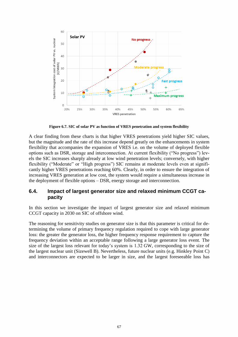
67
Figure 6.7. SIC of solar PV as function of VRES penetration and system flexibility
A clear finding from these charts is that higher VRES penetrations yield higher SIC values,
but the magnitude and the rate of this increase depend greatly on the enhancements in system
flexibility that accompanies the expansion of VRES i.e. on the volume of deployed flexible
options such as DSR, storage and interconnection. At current flexibility (“No progress”) lev-
els the SIC increases sharply already at low wind penetration levels; conversely, with higher
flexibility (“Moderate” or “High progress”) SIC remains at moderate levels even at signifi-
cantly higher VRES penetrations reaching 60%. Clearly, in order to ensure the integration of
increasing VRES generation at low cost, the system would require a simultaneous increase in
the deployment of flexible options – DSR, energy storage and interconnection.
6.4. Impact of largest generator size and relaxed minimum CCGT ca-pacity
In this section we investigate the impact of largest generator size and relaxed minimum
CCGT capacity in 2030 on SIC of offshore wind.
The reasoning for sensitivity studies on generator size is that this parameter is critical for de-
termining the volume of primary frequency regulation required to cope with large generator
loss: the greater the generator loss, the higher frequency response requirement to capture the
frequency deviation within an acceptable range following a large generator loss event. The
size of the largest loss relevant for today’s system is 1.32 GW, corresponding to the size of
the largest nuclear unit (Sizewell B). Nevertheless, future nuclear units (e.g. Hinkley Point C)
and interconnectors are expected to be larger in size, and the largest foreseeable loss has
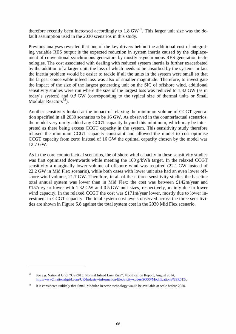
68
therefore recently been increased accordingly to 1.8 GW51
. This larger unit size was the de-
fault assumption used in the 2030 scenarios in this study.
Previous analyses revealed that one of the key drivers behind the additional cost of integrat-
ing variable RES output is the expected reduction in system inertia caused by the displace-
ment of conventional synchronous generators by mostly asynchronous RES generation tech-
nologies. The cost associated with dealing with reduced system inertia is further exacerbated
by the addition of a larger unit, the loss of which needs to be absorbed by the system. In fact
the inertia problem would be easier to tackle if all the units in the system were small so that
the largest conceivable infeed loss was also of smaller magnitude. Therefore, to investigate
the impact of the size of the largest generating unit on the SIC of offshore wind, additional
sensitivity studies were run where the size of the largest loss was reduced to 1.32 GW (as in
today’s system) and 0.5 GW (corresponding to the typical size of thermal units or Small
Modular Reactors52
).
Another sensitivity looked at the impact of relaxing the minimum volume of CCGT genera-
tion specified in all 2030 scenarios to be 16 GW. As observed in the counterfactual scenarios,
the model very rarely added any CCGT capacity beyond this minimum, which may be inter-
preted as there being excess CCGT capacity in the system. This sensitivity study therefore
relaxed the minimum CCGT capacity constraint and allowed the model to cost-optimise
CCGT capacity from zero: instead of 16 GW the optimal capacity chosen by the model was
12.7 GW.
As in the core counterfactual scenarios, the offshore wind capacity in these sensitivity studies
was first optimised downwards while meeting the 100 g/kWh target. In the relaxed CCGT
sensitivity a marginally lower volume of offshore wind was required (22.1 GW instead of
22.2 GW in Mid Flex scenario), while both cases with lower unit size had an even lower off-
shore wind volume, 21.7 GW. Therefore, in all of these three sensitivity studies the baseline
total annual system was lower than in Mid Flex: the cost was between £142m/year and
£157m/year lower with 1.32 GW and 0.5 GW unit sizes, respectively, mainly due to lower
wind capacity. In the relaxed CCGT the cost was £171m/year lower, mostly due to lower in-
vestment in CCGT capacity. The total system cost levels observed across the three sensitivi-
ties are shown in Figure 6.8 against the total system cost in the 2030 Mid Flex scenario.
51 See e.g. National Grid: “GSR015: Normal Infeed Loss Risk”, Modification Report, August 2014,
http://www2.nationalgrid.com/UK/Industry-information/Electricity-codes/SQSS/Modifications/GSR015/.
52 It is considered unlikely that Small Modular Reactor technology would be available at scale before 2030.

69
Figure 6.8. SIC of offshore wind in sensitivity studies on largest unit size and relaxed CCGT capacity in
Mid Flex scenario in 2030
Figure 6.9 summarises the results of SIC studies for these three sensitivities and compares
them against the SIC found in the Mid Flex scenario with the default assumption of 1.8 GW
largest unit size.
Figure 6.9. SIC of offshore wind in sensitivity studies on largest unit size and relaxed CCGT capacity in
Mid Flex scenario in 2030
The impact of reducing the largest unit size to 1.32 GW seems minimal; the CAPEX of ex-
cess offshore wind capacity reduces compared to Base Case, but the system installs slightly
more CCGT which largely offsets lower wind CAPEX resulting in a very similar level of SIC.
With 0.5 GW however there is a visible reduction in SIC from £7.8/MWh to £6.4/MWh,

70
mostly because the biomass plant is utilised less and CCGT more while still meeting the
100 g/kWh target; this is made possible by lower response requirements, allowing the CCGT
generators to operate more efficiently and therefore displace some of the higher marginal cost
biomass output. It could be expected that the reduction of SIC of offshore wind as a conse-
quence of reducing the largest generator size may be more pronounced in a system with
lower flexibility, given that flexible storage and DSR resources allow the system to effi-
ciently cope with higher primary response requirement.
It is also worth mentioning that in the event that new nuclear capacity is not developed in the
2030 horizon, the SIC of VRES technologies may reduce even further, although for exact
quantification it would be necessary to specify assumptions on which technologies would re-
place nuclear in the generation mix.
The impact of relaxed minimum CCGT capacity requirements is also limited, increasing the
SIC of offshore wind by only £0.1/MWh. The slight increase in SIC is the result of the sys-
tem not having excess CCGT capacity in the counterfactual case; therefore more CCGT (and
correspondingly less OCGT) is added when increments in offshore wind capacity are made in
SIC studies.

71
7. Modernised system operation
This chapter discusses potential improvements in system operation that could greatly improve
the efficiency of VRES integration. Some of these improvements have been modelled as part
of Modernisation scenarios.
7.1. Challenges of integrating variable renewables
There are two key factors which may reduce the ability of the system to accommodate the
combination of inflexible low-carbon generation and variable renewables.
(a) A significant increase in system balancing requirements in a decarbonised grid.
- Reserve requirements. Forecasting errors associated with outputs of renewable gen-
eration require appropriate amounts of reserves to be scheduled to ensure that genera-
tion and demand can be balanced at all times. This has an impact on emissions as
conventional plant running to provide reserve will also produce energy, which may
result in curtailment of renewables or reduction in nuclear output, particularly during
low demand periods. The flexibility characteristics of the conventional plant provid-
ing reserve will therefore have a major impact on the emissions performance of the
system. Moreover, when a technology’s generation profile is poorly matched to the
demand profile, plant utilisation across the system is likely to be lower on average,
requiring more capacity to deliver a given level of useful generation (e.g. due to wind
curtailment or reducing nuclear output in summer months). Also, when a particular
technology does not reliably generate at times of peak demand, additional (‘back-up’)
capacity is required to ensure demand can be met at the peak with sufficient level of
security.
- In the studies presented in this report it is assumed that the uncertainty (i.e. forecast-
ing error) of wind output fluctuations is higher than for the output of solar PV genera-
tors, which is in line with the findings in the relevant literature.53
A consequence of
this is that, relative to wind, PV is likely to cause a lower increase in the cost of sys-
tem balancing associated with the provision of longer-term system reserve.
- Response requirements. One of the key contributors to the stability of a power system
is the system inertia54
, which represents the stored energy in the rotating masses of the
synchronous generators and motors. The lower the system inertia, the lower the sys-
tem’s capability to withstand the changes in system frequency. When the majority of
energy supplied to the grid is provided by synchronous machines (such as thermal
plants), there is a high level of system inertia available due to their inherent design.
53 While the short-term (less than 1 hour) variability of diverse wind and solar portfolio is similar in relative terms, the
mid-term (over 1 hour) forecast of PV output is likely to be more accurate than wind. See e.g.:
A. Mills and R. Wiser, “Implications of Wide-Area Geographic Diversity for Short-Term Variability of Solar Power”,
LBNL-38884E, Berkeley, CA: Lawrence Berkeley National Laboratory, 2010.
J. Marcos et al., “Power output fluctuations in large-scale PV plants: One-year observations with one-second resolution
and a derived analytic model”, Progress in Photovoltaics: Research and Applications, vol. 19, pp. 218-227, 2011.
54 System inertia is provided by the rotating masses of turbines in conventional generation plant.

72
However, as the proportion of energy supplied by non-synchronous sources (such as
solar PV, wind and interconnector) increases, the overall system inertia will decrease.
One of the consequences of a reduction in system inertia is an increase in the rate of
change of frequency during frequency incidents (sudden loss/increase of generation or
demand).55
This approach would significantly reduce the efficiency as well as the car-
bon intensity of power system operation.
Wind and solar generators currently do not contribute to system inertia, resulting in
greatly reduced system inertia as the share of renewable generation increases at the
expense of synchronised conventional capacity. The reduction in system inertia on the
other hand increases the system response requirement, and that requires an increased
number of synchronised conventional generators, which would limit the ability to ac-
commodate renewable energy output. The amount of frequency response requirement
for different conditions in the GB system is shown in Figure 7.1.56
The requirement
for frequency response increases sharply during low demand and high wind condi-
tions.
Figure 7.1. Primary frequency response requirement in GB system under different system conditions
The value of frequency regulation in the future GB system is expected to increase
dramatically. This will in turn require that ancillary service markets evolve to recog-
nise the value of different speeds of response, given that the present design is based on
typical response times of conventional power stations.
(b) A lack of flexibility in the present system. Present conventional gas and coal generators are relatively inflexible, particularly in
terms of limited amount of frequency control that can be provided and relatively high
55 In this context, National Grid is considering updating frequency regulation standards, particularly the rate of change of
frequency (RoCoF), which will be beneficial in enhancing the ability of the system to accommodate increased levels of
renewable generation.
56 F. Teng, V. Trovato and G. Strbac, “Stochastic Scheduling with Inertia-dependent Fast Frequency Response Require-
ments”, IEEE Transaction on Power Systems, issue 99, 2015.

73
minimum stable generation. These two features represent the key limiting factors for
the amount of renewable generation that can be accommodated, given that, unless al-
ternative service providers emerge, a significant volume of conventional generation
will need to operate in order to deliver the required level of balancing services, while
at the same time injecting energy into the grid that may not be required during high
renewable output periods. There is also a limited amount of demand-side response
services that can support system balancing in the timeframe from seconds to hours. In
the future however, system flexibility may significantly improve. In this context, an
update of market arrangements to reward different forms of flexibility will be impor-
tant57
. For example, conventional generation technologies of significantly enhanced
flexibility are already available, but power companies do not presently find it attrac-
tive to make corresponding investments. Similarly, energy storage technologies and
demand-side response could significantly enhance system flexibility. Finally,
strengthening the interconnection with the EU electricity system can also bring sys-
tem integration benefits.
Therefore, a combination of low demand, high renewables output, and high output of must-
run units such as nuclear plants, or conventional generators that have to be synchronised in
order to provide frequency regulation will have an adverse impact the carbon intensity of the
electricity system (as the curtailed renewables output needs to be compensated by increased
energy from mid-merit fossil fuel-based power plant).
To enable the system to accommodate cost effectively low-carbon electricity and therefore
achieve decarbonisation targets, successively enhancing system flexibility to will be critical.
Flexible options considered include:
More efficient and more flexible generation technologies: conventional plant that
can operate stably at lower levels of output (and therefore less likely to push renew-
ables out of system) and provide faster frequency response (requiring less overall
thermal plant to be built to balance the system).
Provision of frequency regulation by wind generation – it is expected that future
wind generation technologies will be capable of providing ancillary services, includ-
ing inertia.
Deployment of energy storage (e.g. battery technologies) and Demand-side re-
sponse would support short-term operation as well as provide primary and secondary
frequency response and security of supply and reduce the need for additional back-up
generation and network infrastructure reinforcement.
Increased interconnection with mainland Europe.
57 National Grid has recently introduced additional frequency regulation products that should encourage provision of en-
hanced response services and hence increase the ability of the system to accommodate low carbon generation.

74
7.2. Market value of energy and ancillary services in future systems
In this section we present several results from previous studies to show the magnitude of ex-
pected change in the system operating cost associated with energy delivery and the operating
cost associated with ancillary services.
Given that key low-carbon generation technologies such as wind, PV or nuclear have very
low operating costs, the operating cost associated with delivering energy is expected to de-
crease going forward. At the same time, the cost associated with the provision of ancillary
services is likely to increase substantially driven by both increased requirements for fre-
quency regulation as well as the cost of managing wind uncertainty. Similarly, the volume of
the capacity market is expected to increase several times as new generators start participating
in the market. The increasing prominence of ancillary service and capacity markets will cre-
ate opportunities for flexible providers such as energy storage and DSR to fulfil their com-
mercial potential and contribute to system operation.
Figure 7.2 illustrates this point by providing an estimate of operating cost associated with en-
ergy delivery and the cost of providing ancillary services (reserve and response), for two
wind penetrations: 1) 10 GW, which is close to today’s installed wind capacity, and
2) 50 GW, which is closer to expected wind capacity in 2030. The figure shows that energy
cost would broadly drop by 50%, while the cost of ancillary services would increase order of
magnitude. The share of ancillary service cost in the total operating cost will increase from
about 1-2% to more than 25%. Note that these costs have been estimated based on today’s
carbon and energy prices; imposing higher carbon prices would increase the total cost, how-
ever the relative proportions of energy and ancillary service costs would remain the same.
Figure 7.2. Operating cost associated with energy and ancillary services for different wind penetration
levels
7.3. Enhancing market and regulatory framework to facilitate de-ployment of energy storage and DSR
Actual realisation and deployment of flexible options will require significant enhancement of
the market and regulatory framework to facilitate the delivery of adequate levels of flexibility.

75
In the context of DSR and storage, it is important to bear in mind that the method of cost
minimisation used in this work is equivalent to assuming that investment decisions are taken
in a perfectly competitive market, while in reality, market failures, such as the impact of ex-
ternalities, inefficient pricing or natural monopoly, mean that the least-cost level of deploy-
ment might not take place in practice.
Furthermore, previous analyses have also clearly demonstrated that DSR and storage can
bring benefits to several sectors in electricity industry, including generation, transmission and
distribution, while providing services to support real time balancing of demand and supply
and network congestion management and reduce the need for investment in system rein-
forcement. These “split benefits” of storage end DSR pose significant challenges for policy
makers to develop appropriate market mechanisms to ensure that the investors in storage and
DSR are adequately rewarded for delivering these diverse sources of value.
It is not clear whether government policies should incentivise the development and deploy-
ment of novel storage technologies, and if so, what sort of mechanisms should be considered,
e.g. ranging from subsidies to direct procurement.
7.4. Opportunities and barriers for gas plant of enhanced flexibility
There is expectation that new gas plant will be connected to the UK system to replace coal-
based power generation that is being decommissioned. Given the expected growth in variable
renewable and inflexible nuclear generation, our analysis demonstrates that it would be bene-
ficial to connect gas plant with enhanced flexibility. The flexibility parameters associated
with thermal plants, combined cycle gas plant (CCGT) in particular include:
Ramp rates describe the speed at which the plant can change its output between the
minimum and maximum load levels and is generally expressed as percentage of the
maximum capacity per minute. Typical maximum ramp rate for the present CCGT
plants is around 4%/min.
Minimum stable generation is defined as the lowest level that a plant can continu-
ously operate and is expressed as a percentage of the maximum capacity. Due to
the MSG constraint, provision of the synchronized balancing services is inevitably
accompanied by the delivery of electricity production, which may lead to a large
amount of RES curtailment during low demand and high RES periods. At present,
MSG of CCGT plant is limited at around 50%, while the latest design of Alstom
CCGT plant is expected to be capable of continuously operating at around 20-30%
of nominal power.
Frequency response capability is defined by two parameters, maximum response
and response slope. Due to limited inertia capability of RES, the frequency re-
sponse requirements are expected to increase significantly in the future low carbon
systems, leading to a higher demand on the frequency response contribution from
thermal plants. Figure 7.3 shows present response characteristics of a CCGT plant
as well as potentially enhanced characteristics.

76
Figure 7.3. Frequency response characteristics of CCGT plant
Part-load Efficiency - is defined as the ratio of the efficiency at part-load operation
over the efficiency at full-load operation. As the increased requirements on ramping,
operating reserve and frequency response in the future low carbon system, part-load
operation of thermal plant will become more common in order to provide these ser-
vices, leading to a degraded system economic and environmental performance.
Significant work has been conducted to enhance the part load efficiency of CCGT
plant; improved part-load efficiency curve of CCGT plant are shown in Figure 7.4.
Figure 7.4. Typical part-load efficiency curve of a CCGT plant
Start-up Time - describes the time the plant takes to start generating electricity and
this is highly depends on amount of time that elapsed since its last shutdown. Start-
up times of conventional CCGT is 2-4 hours while more flexible plant would be
synchronised within 50% of this time. In the future, the variability of RES would
increase the number of start-ups of thermal plants and the uncertainty of RES
would increase the challenge of making start-up decision long time ahead of real-
time operation. The start-up decision of a thermal plant with shorter start-up time
could be made nearer to real-time operation, which significantly reduces the uncer-
tainty faced by the operator.
The marginal system value of CCGTs with enhanced flexibility is shown in Figure 7.5. The
value of the first 5 GW CCGTs with enhanced flexibility is above £1,000/kW, and reduces to
£300/kW for the second 5 GW. Given that cost of CCGTs with enhance flexibility will be
larger, the market volume for such plant is presented by this figure.

77
Figure 7.5. Value of flexible generation
Further analysis was carried out to determine the impact of gas plant with enhanced flexibil-
ity on the operating patterns of less flexible generation, which is presented in Figure 7.6.
Figure 7.6. Changes in electricity output of generation technologies
Clearly, the presence of CCGT with enhanced flexibility would increase the production of
nuclear and wind generation, but also of inflexible CCGTs, making significant cost and emis-
sions benefits. As expected, this would also reduce the energy production of the flexible
when compared with inflexible CCGT. Given that the present market rewards energy produc-
tion rather than flexibility, it is not clear if the investment in flexible generation would mate-
rialise, as the investors may not capture system benefits delivered by the flexible plants (that
is obviously characterised with higher cost than inflexible). Market designs would need to be
developed in order to provide right signal for the market players to invest in flexible genera-
tion.
0
200
400
600
800
1000
1200
5 10 15
Value(£/kW)
Capacity(GW)
-0.5
-0.4
-0.3
-0.2
-0.1
0
0.1
0.2
0.3
0.4
0.5
EnergyChanges(TW
h)
OCGT
CCGT_Flex
CCGT_Base
Nuclear
Wind
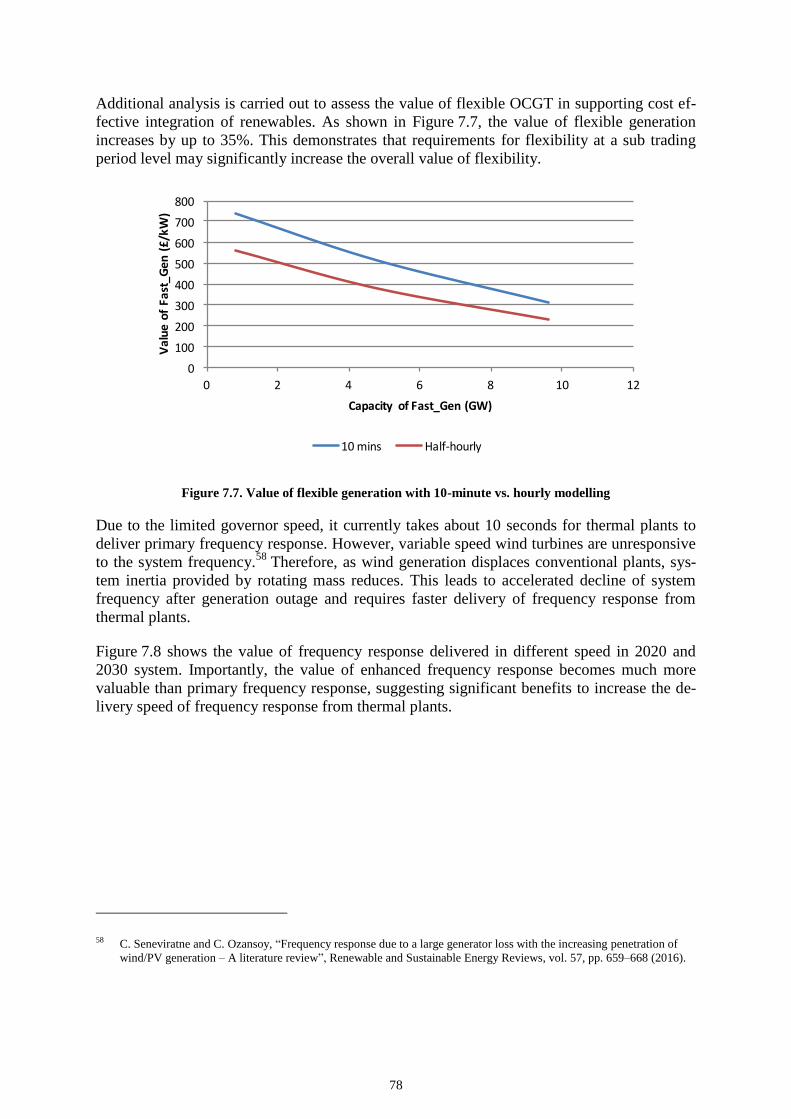
78
Additional analysis is carried out to assess the value of flexible OCGT in supporting cost ef-
fective integration of renewables. As shown in Figure 7.7, the value of flexible generation
increases by up to 35%. This demonstrates that requirements for flexibility at a sub trading
period level may significantly increase the overall value of flexibility.
Figure 7.7. Value of flexible generation with 10-minute vs. hourly modelling
Due to the limited governor speed, it currently takes about 10 seconds for thermal plants to
deliver primary frequency response. However, variable speed wind turbines are unresponsive
to the system frequency.58
Therefore, as wind generation displaces conventional plants, sys-
tem inertia provided by rotating mass reduces. This leads to accelerated decline of system
frequency after generation outage and requires faster delivery of frequency response from
thermal plants.
Figure 7.8 shows the value of frequency response delivered in different speed in 2020 and
2030 system. Importantly, the value of enhanced frequency response becomes much more
valuable than primary frequency response, suggesting significant benefits to increase the de-
livery speed of frequency response from thermal plants.
58 C. Seneviratne and C. Ozansoy, “Frequency response due to a large generator loss with the increasing penetration of
wind/PV generation – A literature review”, Renewable and Sustainable Energy Reviews, vol. 57, pp. 659–668 (2016).
0
100
200
300
400
500
600
700
800
0 2 4 6 8 10 12
ValueofFast_Gen(£/kW)
CapacityofFast_Gen(GW)
10mins Half-hourly

79
Figure 7.8. Value of primary frequency response and enhanced frequency response
7.5. Enhancing EU market design to facilitate cross-border energy, capacity and reserve trading
Benefits of moving from the current member state-centric to a pan-Europe wide market de-
sign would be very significant. Analysis demonstrated that the benefits of fully integrating
EU energy and capacity markets would be €12-40bn/year and €7-10bn/year respectively by
2030, while integration of the EU balancing market would save an additional €3-5bn/year.
These savings go far beyond the €2.5-4bn/year that the EU has saved through its existing
measures to integrate its electricity markets through day-ahead energy arbitrage.
Under high levels of penetration of variable renewable generation, the operating reserve re-
quirements and need for flexibility increase significantly. In particular, the allocation of the
reserve portfolio between spinning and standing products is vital to operate a congested net-
work efficiently. This is because the commitment of spinning reserves in areas with signifi-
cant wind generation can be very costly due to potential wind curtailment events. In such
cases, the commitment of standing reserves should be preferred over spinning reserve, even if
these are located in neighbouring states and may require reduction in network energy trans-
fers leading to increase in constraints cost. In such cases, the need to access the optimum
portfolio of reserves has to be balanced against the need to access low-cost energy sources,
leading to the allocation of interconnection capacity between energy delivery and reserve ser-
vices. Although the question of allocating network capacity between energy and reserve is a
key issue, it is not facilitate by the current market coupling arrangements.
In Figure 7.9 below, an example of a two-area system is presented – Area A with significant
penetration of renewables (e.g. UK) and Area B with significant penetration of low cost gen-
eration, such as nuclear, but also flexible standing generation (e.g. France). If we ignore the
reserve requirement, the interconnector capacity will be used for transport of energy from
Area B to Area A. However, if the interconnector capacity is optimised between energy and
reserve, we observe that flows between the two areas will be radically different.
0
500
1000
1500
2000
2500
2020 2030
Value(£/kW/Year)
PrimaryFrequencyResponseProvision EnhancedPrimaryFrequencyResponseProvision

80
Figure 7.9. Allocation of interconnection capacity between trading energy and reserve services
Clearly, the development of new trading arrangements for sharing reserve between member
states would bring significant benefits, particularly to the UK.59
It will be important to opti-
mise allocation of reserve products across regions, as there are potentially significant benefits
of sharing flexibility that can be achieved by shifting the requirements to provide reserve
from areas with high renewable production (exporting areas) to areas with low production or
demand-dominated areas (importing areas) by making use of cross-border transmission. Fur-
thermore, given the increased diversity in demand and renewable output across intercon-
nected areas, when reserve products are shared across member states, rather than every mem-
ber state providing reserve services for its own needs, the total reserve requirements are
bound to decrease substantially. Recent analysis of the annual operation of the EU system
shows that regional sharing of frequency regulation and reserve services using cross-border
capacity reduces operating costs by about €3bn/annum, when compared with a policy where
each member state provides the services to meet their own requirements. When considering
carbon impacts, these benefits can be very significant for the UK.
However, the present market arrangements do not facilitate the optimal allocation of inter-
connection capacity between energy and reserve services. Transmission capacity in Europe is
currently allocated by power exchanges trading energy, while separate institutions deal with
reserve and balancing. This is an issue of high priority that should be resolved at the Euro-
pean level through design of efficient market mechanisms to ensure optimal resource sharing
across all Member States.
59 G. Strbac, M. Aunedi, D. Pudjianto, P. Djapic, S. Gammon and R. Druce, Understanding the Balancing Challenge,
DECC, 2012.
0
1
2
3
0
5
10
15
20
25
30
1
10
19
28
37
46
55
64
73
82
91
100
109
118
127
136
145
154
163
172
181
190
199
208
217
226
235
244
253
262
271
280
289
298
307
316
325
334
Powerflow(GW)
WindPower(GW)
WindPower ReservepurchasedinA ReservepurchasedinB

81
8. Conclusions
In this report we have quantified system integration cost of low-carbon generation technolo-
gies across different future development scenarios. Key findings from quantitative studies
include:
Total annualised system cost for the 2030 GB system with the carbon intensity of
100 g/kWh will be driven by system flexibility. Up to £4.2bn/year could be saved by
improving system flexibility from today’s level; most of these savings are already
achievable with moderately enhanced flexibility.
The SIC of variable RES generation is strongly dependent on system flexibility as
well as on the overall energy mix (i.e. the penetration of variable RES) and is there-
fore a function of assumed system evolution. As illustrated in Figure 8.1 on the exam-
ple of SIC values obtained for onshore wind, higher VRES penetrations yield a higher
SIC, but the magnitude and the rate of this increase depends greatly on the level of
enhancements in system flexibility that accompanies the expansion of VRES i.e. on
the volume of deployed flexible options such as DSR, storage and interconnection.
The figure identifies trend lines for four different rates of deployment of flexibility
(No, Moderate, Fast and Maximum progress). At current flexibility (“No progress”)
levels the SIC increases sharply already at low wind penetration levels; conversely,
with higher flexibility (“Moderate” or “High progress”) SIC remains at moderate lev-
els even at significantly higher VRES penetrations.
Figure 8.1. SIC of onshore wind as function of wind penetration
System integration cost of wind and solar PV generation in the 2030 horizon remains
at a moderate level provided that the assumed enhancement of system flexibility ma-
terialises (i.e. that there is a rapid deployment of energy storage and DSR). In addition
to system flexibility, the SIC of variable RES generation is also strongly dependent on
the overall energy mix and is therefore a function of assumed system evolution.

82
SIC of both offshore and onshore wind in 2030 (when compared against nuclear
power) is found to be around £5-9/MWh across the medium to high flexible scenarios
analysed in the study. The majority of this cost is associated with the requirement to
build sufficient firm (back-up) capacity when wind is added to the system, in order to
maintain the same level of security of supply. A smaller part of SIC of wind is associ-
ated with increased operating cost resulting from increased requirement for ancillary
services triggered by added wind capacity.
In a system with no added flexibility compared to today’s situation, the SIC of vari-
able RES technologies would increase beyond £40/MWh, making it very costly to in-
tegrate large penetrations of variable renewables.
SIC of solar PV generation in 2030 is slightly higher than for offshore wind, and var-
ies within the £10-15/MWh range with medium flexibility assumptions. When com-
pared to offshore wind, it contains an additional component associated with distribu-
tion investment cost, given that large volumes of PV, especially if they are not in-
stalled uniformly across GB (as assumed in the study), may trigger distribution net-
work reinforcement to deal with increased reverse power flows i.e. electricity being
injected back into the distribution grid.
According to the LCOE assumptions adopted in the study, despite the positive SIC the
whole-system cost of offshore and onshore wind and PV (i.e. the sum of their LCOE
and SIC) still makes them competitive to nuclear in the majority of 2030 scenarios
with at least moderate flexibility (the only exception is Nuclear Centric scenario
where nuclear represents a more economical choice given the more favourable LCOE
assumptions in that scenario).
Despite an increasing penetration of variable renewables between 2015 and 2030, SIC
of wind and PV can be maintained at a relatively stable level (or even lower in some
scenarios) provided that sufficient amount of flexible options is deployed. This occurs
because the impact of increasing RES penetration, creating an upward pressure on
SIC, is counteracted by the opposing impact of improved flexibility.
Increasing or reducing system flexibility has a critical impact on the total system cost
required to meet the 2030 carbon target, as well as on SIC of variable RES. The inte-
gration of variable RES in a system with scarce flexibility would be very costly and
inefficient, requiring about £4bn/year more to meet the 100 g/kWh target than in the
five core scenarios. Nevertheless, a moderate improvement of system flexibility al-
ready brings the cost of the system down by £3.5bn/year, while at the same time re-
ducing SIC of offshore and onshore wind from over £40/MWh down to around
£11/MWh in the 2030 horizon. This level of SIC combined with the LCOE assump-
tions makes offshore and particularly onshore wind cost-effective compared to nu-
clear generation. Flexibility levels towards the high level of the spectrum will require
coordinated action and policy support starting from today in order to ensure high vol-
umes of flexible options are deployed over the next decade or so.
Sensitivity studies carried out for 2030 scenarios with a more ambitious carbon target
of 50 /kWh suggest that the integration cost of VRES would increase, driven primar-
ily by higher RES penetration required to meet the lower emission target. In some in-

83
stances, like in Mid Flex and Onshore Capped scenarios, where the penetration of
wind exceeds 55% of annual electricity demand, any integration of further wind ca-
pacity becomes very costly. Such high levels of wind require further improvements in
system flexibility or operation practices, such as those assumed in Modernisation or
Mega Flex scenarios.

84
Appendix A. Overview of the methodology for whole-system analysis of electricity systems
In this section we describe our approach and models used to quantify the system integration
cost of low-carbon generation technologies in future electricity systems. We highlight the key
capabilities of our novel modelling framework, which enables a holistic economic assessment
of electricity systems that include alternative balancing technologies. This framework makes
optimal operation and investment decisions aimed at minimising the total system cost, by
trading off short-term operating decisions against those related to long-term investment into
new generation, transmission and distribution networks or storage capacity.
We first highlight the necessity to adopt a whole-systems approach when assessing the value
of flexible balancing technologies in future low-carbon electricity systems, and describe Im-
perial’s Whole-electricity System Investment Model (WeSIM), which is specifically designed
to perform this type of analysis. We also present our approach to estimating the distribution
reinforcement cost at the national scale, using the concept of statistically representative net-
works. The description of our modelling approach is concluded with the overview of flexible
demand technologies considered in studying the impact of demand-side response. This in-
volves a number of different demand technologies, each of which is studied in detail using
dedicated bottom-up models that enable us to quantify the flexibility potentially provided by
these technologies, while maintaining the level and quality of service provided to end con-
sumers.
Our approach to quantifying the value of flexible balancing technologies considers total sys-
tem cost (including both investment and operation) for a given generation and demand sce-
nario, and compares the case when the model is allowed to add new capacity of alternative
balancing technologies (such as interconnection, flexible generation, storage or DSR) in a
cost-optimal manner, with the case where no such addition is allowed in the system. The re-
duction in total system cost as a result of deploying flexible balancing technologies is inter-
preted as the value generated by these technologies, which also takes into account the in-
vestment needed to build the new capacity of flexible technologies.
A.1. Whole-systems modelling of electricity sector
When considering system benefits of enabling technologies such as storage, Demand-Side
Response (DSR), interconnection and flexible generation, it is important to consider two key
aspects:
Different time horizons: from long-term investment-related time horizon to real-time
balancing on a second-by-second scale (Figure A.1); this is important as the alterna-
tive balancing technologies can both contribute to savings in generation and network
investment as well as increasing the efficiency of system operation.
Different assets in the electricity system: generation assets (from large-scale to dis-
tributed small-scale), transmission network (national and interconnections), and local
distribution network operating at various voltage levels. This is important as alterna-
tive balancing technologies may be placed at different locations in the system and at
different scales. For example, bulk storage is normally connected to the national

85
transmission network, while highly distributed technologies may be connected to lo-
cal low-voltage distribution networks.
Figure A.1. Balancing electricity supply and demand across different time horizons
Capturing the interactions across different time scales and across different asset types is es-
sential for the analysis of future low-carbon electricity systems that includes alternative bal-
ancing technologies such as storage and demand side response. Clearly, applications of those
technologies may improve not only the economics of real time system operation, but they can
also reduce the investment into generation and network capacity in the long-run.
In order to capture these effects and in particular trade-offs between different flexible tech-
nologies, it is critical that they are all modelled in a single integrated modelling framework.
In order to meet this requirement we have developed WeSIM, a comprehensive system analy-
sis model that is able to simultaneously balance long-term investment decisions against short-
term operation decisions, across generation, transmission and distribution systems, in an inte-
grated fashion.
This holistic model provides optimal decisions for investing into generation, network and/or
storage capacity (both in terms of volume and location), in order to satisfy the real-time sup-
ply-demand balance in an economically optimal way, while at the same time ensuring effi-
cient levels of security of supply. The WeSIM has been extensively tested in previous pro-
jects studying the interconnected electricity systems of the UK and the rest of Europe.60
An
advantage of WeSIM over most traditional models is that it is able to simultaneously consider
system operation decisions and capacity additions to the system, with the ability to quantify
trade-offs of using alternative mitigation measures, such as DSR and storage, for real-time
balancing and transmission and distribution network and/or generation reinforcement man-
agement. For example, the model captures potential conflicts and synergies between different
applications of distributed storage in supporting intermittency management at the national
level and reducing necessary reinforcements in the local distribution network.
60 WeSIM model, in various forms, has been used in a number of recent European projects to quantify the system infra-
structure requirements and operation cost of integrating large amounts of renewable electricity in Europe. The projects
include: (i) “Roadmap 2050: A Practical Guide to a Prosperous, Low Carbon Europe” and (ii)“Power Perspective 2030:
On the Road to a Decarbonised Power Sector”, both funded by European Climate Foundation (ECF); (iii) “The revision
of the Trans-European Energy Network Policy (TEN-E)” funded by the European Commission; and (iv) “Infrastructure
Roadmap for Energy Networks in Europe (IRENE-40)” funded by the European Commission within the FP7 pro-
gramme.
Generation, Transmission &
Distribution Planning
Long-term Generation and Storage Scheduling
Day-ahead Generation,
Storage & DSR Scheduling
System Balancing
Actual delivery: physical generation & consumption
One day to one hour before
delivery
Months to days before delivery
Years before delivery
Adequacy Reserve & ResponseArbitrage
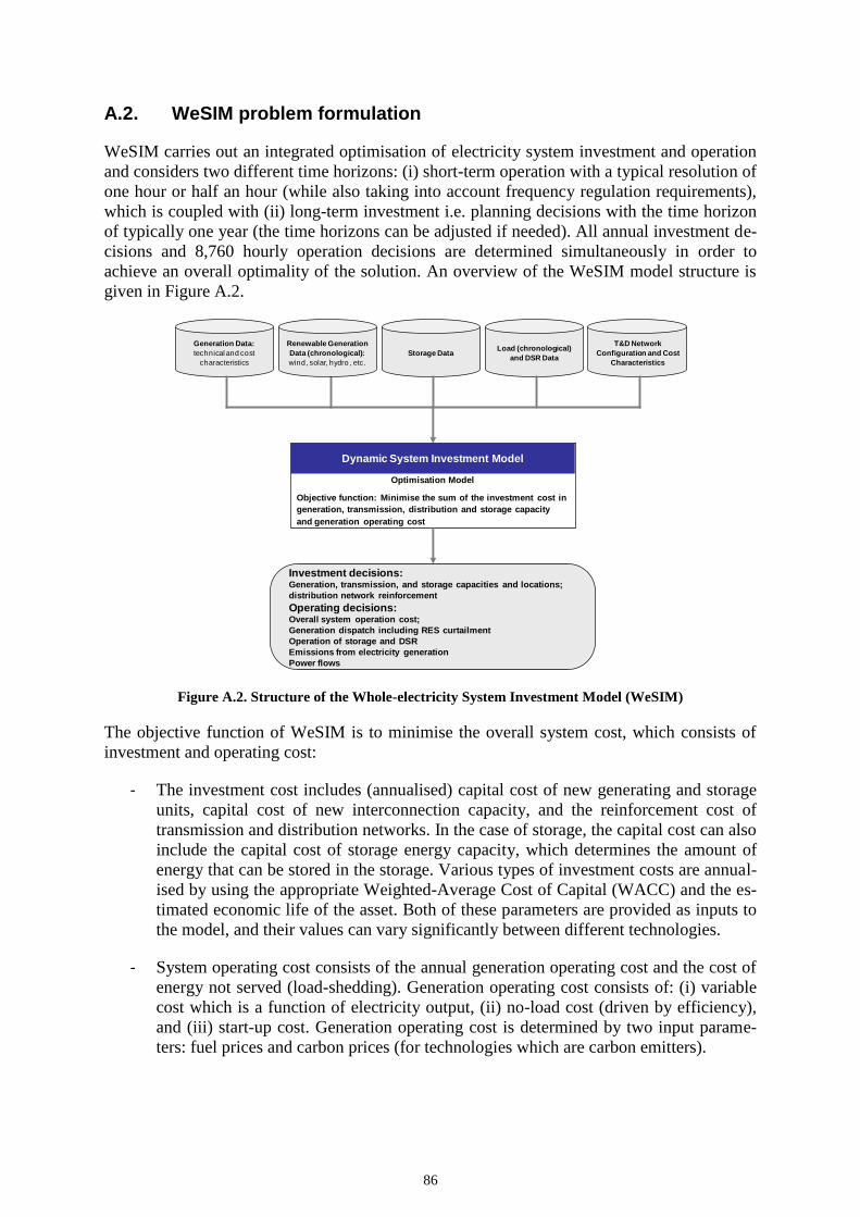
86
A.2. WeSIM problem formulation
WeSIM carries out an integrated optimisation of electricity system investment and operation
and considers two different time horizons: (i) short-term operation with a typical resolution of
one hour or half an hour (while also taking into account frequency regulation requirements),
which is coupled with (ii) long-term investment i.e. planning decisions with the time horizon
of typically one year (the time horizons can be adjusted if needed). All annual investment de-
cisions and 8,760 hourly operation decisions are determined simultaneously in order to
achieve an overall optimality of the solution. An overview of the WeSIM model structure is
given in Figure A.2.
Figure A.2. Structure of the Whole-electricity System Investment Model (WeSIM)
The objective function of WeSIM is to minimise the overall system cost, which consists of
investment and operating cost:
- The investment cost includes (annualised) capital cost of new generating and storage
units, capital cost of new interconnection capacity, and the reinforcement cost of
transmission and distribution networks. In the case of storage, the capital cost can also
include the capital cost of storage energy capacity, which determines the amount of
energy that can be stored in the storage. Various types of investment costs are annual-
ised by using the appropriate Weighted-Average Cost of Capital (WACC) and the es-
timated economic life of the asset. Both of these parameters are provided as inputs to
the model, and their values can vary significantly between different technologies.
- System operating cost consists of the annual generation operating cost and the cost of
energy not served (load-shedding). Generation operating cost consists of: (i) variable
cost which is a function of electricity output, (ii) no-load cost (driven by efficiency),
and (iii) start-up cost. Generation operating cost is determined by two input parame-
ters: fuel prices and carbon prices (for technologies which are carbon emitters).
Generation Data:
technical and cost
characteristics
Renewable Generation
Data (chronological):
wind, solar, hydro , etc.
Storage DataLoad (chronological)
and DSR Data
T&D Network
Configuration and Cost
Characteristics
Dynamic System Investment Model
Optimisation Model
Objective function: Minimise the sum of the investment cost in
generation, transmission, distribution and storage capacity
and generation operating cost
Investment decisions: Generation, transmission, and storage capacities and locations;
distribution network reinforcement
Operating decisions:Overall system operation cost;
Generation dispatch including RES curtailment
Operation of storage and DSR
Emissions from electricity generation
Power flows

87
There are a number of equality and inequality constraints that need to be respected by the
model while minimising the overall cost. These include:
- Power balance constraints, which ensure that supply and demand are balanced at all
times.
- Operating reserve constraints include various forms of fast and slow reserve con-
straints. The amount of operating reserve requirement is calculated as a function of
uncertainty in generation and demand across various time horizons. The model distin-
guishes between two key types of balancing services: (i) frequency regulation (re-
sponse), which is delivered in the timeframe of a few seconds to 30 minutes; and (ii)
reserves, typically split between spinning and standing reserve, with delivery occur-
ring within the timeframe of tens of minutes to several hours after the request (this is
also linked with need to re-establish frequency regulation services following outage of
a generating plant). The need for these services is also driven by wind output forecast-
ing errors and this will significantly affect the ability of the system to absorb wind en-
ergy. It is expected that the 4 hour ahead61
forecasting error of wind, being at present
at about 15% of installed wind capacity, may reduce to 10% post-2020 and then fur-
ther to less than 6%, may have a material impact of the value of flexibility options.
Calculation of reserve and response requirements for a given level of variable renew-
able generation is carried out exogenously and provided as an input into the model.
WeSIM then schedules the optimal provision of reserve and response services, taking
into account the capabilities and costs of potential providers of these services (re-
sponse slopes, efficiency losses of part loaded plant etc.) and finding the optimal
trade-off between the cost of generating electricity to supply a given demand profile,
and the cost of procuring sufficient levels of reserve and response (this also includes
alternative balancing technologies such as storage and DSR as appropriate).
In order to take into account the impact of having less inertia during low demand and
high renewable output conditions, the WeSIM’s formulation has been enhanced by
including additional constraints that dictate the minimum response requirements to
meet the RoCOF specification, the minimum frequency at the nadir point, and the
steady state frequency deviation from the nominal frequency as illustrated in Fig-
ure A.3.
61 4 hours is generally the maximum time needed to synchronize a large CCGT plant.

88
Figure A.3. System frequency evolution after a contingency (source: National Grid)
In WeSIM, frequency response can be provided by:
o Synchronised part-loaded generating units.
o Interruptible charging of electric vehicles.
o A proportion of wind power being curtailed.
o A proportion of electricity storage when charging
o Smart refrigeration.
While reserve services can be provided by:
o Synchronised generators
o Wind power or solar power being curtailed
o Stand-by fast generating units (OCGT)
o Electricity storage
o I&C flexible demand
o Interruptible heat storage when charging
The amount of spinning and standing reserve and response is optimized ex-ante to
minimise the expected cost of providing these services, and we use our advanced sto-
chastic generation scheduling models to calibrate the amount of reserve and response
scheduled in WeSIM.62,63
These models find the cost-optimal levels of reserve and re-
sponse by performing a probabilistic simulation of the actual utilisation of these ser-
vices. Stochastic scheduling is particularly important when allocating storage re-
sources between energy arbitrage and reserve as this may vary dynamically depending
on the system conditions.
62 A. Sturt, G. Strbac, “Efficient Stochastic Scheduling for Simulation of Wind-Integrated Power Systems”, IEEE Trans-
actions on Power Systems, Vol: 27, pp. 323-334, Feb 2012.
63 A. Sturt, G. Strbac, “Value of stochastic reserve policies in low-carbon power systems”, Proceedings of the Institution
of Mechanical Engineers: Part O-Journal of Risk and Reliability, Vol: 226, pp. 51-64, Feb 2012.
1
RoCoF
Freq. at
nadir
Steady-
state freq.

89
- Generator operating constraints include: (i) Minimum Stable Generation (MSG) and
maximum output constraints; (ii) ramp-up and ramp-down constraints; (ii) minimum
up and down time constraints; and (iv) available frequency response and reserve con-
straints. In order to keep the size of the problem manageable, we group generators ac-
cording to technologies, and assume a generic size of a thermal unit of 500 MW (the
model can however commit response services to deal with larger losses, e.g.
1,800 MW as used in the model). The model captures the fact that the provision of
frequency response is more demanding than providing operating reserve. Only a pro-
portion of the headroom created by part-loaded operation, as indicated in Figure A.4.
- Given that the functional relationship between the available response and the reduced
generation output has a slope with an absolute value considerably lower than 1, the
maximum amount of frequency regulation that a generator can provide (Rmax) is gen-
erally lower than the headroom created from part-loaded operation (Pmax – MSG).
Figure A.4. Provision of frequency regulation from conventional generation
- Generation: WeSIM optimises the investment in new generation capacity while con-
sidering the generators’ operation costs and CO2 emission constraints, and maintain-
ing the required levels of security of supply. WeSIM optimises both the quantity and
the location of new generation capacity as a part of the overall cost minimisation. If
required, the model can limit the investment in particular generation technologies at
given locations.
- Annual load factor constraints can be used to limit the utilisation level of thermal
generating units, e.g. to account for the effect of planned annual maintenance on plant
utilisation.
- For wind, solar, marine, and hydro run-of-river generators, the maximum electricity
production is limited by the available energy profile, which is specified as part of the
input data. The model will maximise the utilisation of these units (given zero or low
marginal cost). In certain conditions when there is oversupply of electricity in the sys-
tem or reserve/response requirements limit the amount of renewable generation that
can be accommodated, it might become necessary to curtail their electricity output in
order to balance the system, and the model accounts for this.
- For hydro generators with reservoirs and pumped-storage units, the electricity pro-
duction is limited not only by their maximum power output, but also by the energy
available in the reservoir at a particular time (while optimising the operation of stor-

90
age). The amount of energy in the reservoir at any given time is limited by the size of
the reservoir. It is also possible to apply minimum energy constraints in WeSIM to
ensure that a minimum amount of energy is maintained in the reservoir, for example
to ensure the stability of the plant. For storage technologies, WeSIM takes into ac-
count efficiency losses.
- Demand-side response constraints include constraints for various specific types of
loads. WeSIM broadly distinguishes between the following electricity demand catego-
ries: (i) weather-independent demand, such as lighting and industrial demand, (ii)
heat-driven electricity demand (space heating / cooling and hot water), (iii) demand
for charging electric vehicles, and (iv) smart appliances’ demand. Different demand
categories are associated with different levels of flexibility. Losses due to temporal
shifting of demand are modelled as appropriate. Flexibility parameters associated with
various forms of DSR are obtained using detailed bottom-up modelling of different
types of flexible demand, as described in the “Demand modelling” section.
- Power flow constraints limit the energy flowing through the lines between the areas in
the system, respecting the installed capacity of network as the upper bound (WeSIM
can handle different flow constraints in each flow direction). The model can also in-
vest in enhancing network capacity if this is cost efficient. Expanding transmission
and interconnection capacity is generally found to be vital for facilitating efficient in-
tegration of large amounts of variable renewable resources, given their location. Inter-
connectors provide access to renewable energy and improve the diversity of demand
and renewable output on both sides of the interconnector, thus reducing the short-term
reserve requirement. Interconnection also allows for sharing of reserves, which re-
duces the long-term capacity requirements.
- Distribution network constraints are devised to determine the level of distribution
network reinforcement cost, as informed by detailed modelling of representative UK
networks. WeSIM can model different types of distribution networks, e.g. urban, rural,
etc. with their respective reinforcement cost (more details on the modelling of distri-
bution networks are provided in the section “Distribution network investment model-
ling”).
- Emission constraints limit the amount of carbon emissions within one year. Depend-
ing on the severity of these constraints, they will have an effect of reducing the elec-
tricity production of plants with high emission factors such as oil or coal-fired power
plants. Emission constraints may also result in additional investment into low-carbon
technologies such as renewables (wind and PV), nuclear or CCS in order to meet the
constraints.
- Security constraints ensure that there is sufficient generating capacity in the system to
supply the demand with a given level of security.64
If there is storage in the system,
WeSIM may make use its capacity for security purposes if it can contribute to reduc-
ing peak demand, given the energy constraints.
64 Historical level of security supply are achieved by setting VOLL at around 10,000£/MWh.

91
WeSIM allows for the security-related benefits of interconnection to be adequately
quantified.65
Conversely, it is possible to specify in WeSIM that no contribution to se-
curity is allowed from other regions, which will clearly increase the system cost, but
will also provide an estimate of the value of allowing the interconnection to be used
for sharing security between regions.
Specific constraints implemented in WeSIM for the purpose of studying balancing technolo-
gies are:
- UK is self-sufficient in terms of capacity, i.e. there is no contribution from other re-
gions to the capacity margin in the UK and vice versa. However, sensitivity studies
are carried out to understand the impact of relaxing the self-sufficient constraint on
the cost of making the system secure and the value of alternative balancing technolo-
gies in supporting the system.
- UK is energy-neutral. This means that the net annual energy import / export is zero.
This allows UK to import power from and export to Europe / Ireland as long as the
annual net balance is zero. In other words, the UK is still able to export power when
there is excess in energy available, for example when high wind conditions coincide
with low demand, and import energy from Europe when economically efficient e.g.
during low-wind conditions in UK.
A.3. System topology
The configuration of the interconnected GB electricity system used in this study is presented
in Figure A.5. Given that the GB transmission network is characterised by North-South
power flows, it was considered appropriate to represent the GB system using the four key re-
gions and their boundaries, while considering London as a separate zone.
The two neighbouring systems, Ireland and Continental Europe (CE), are considered (CE is
an equivalent representation of the entire interconnected European system). Several genera-
tion and demand backgrounds in CE and Ireland are considered (for example, WeSIM opti-
mises the operation of the entire European system, including seasonal optimisation hydro in
Scandinavia, pump storage schemes across CE and DSR across CE).
Lengths of the network in Figure A.5 do not reflect the actual physical distances between dif-
ferent areas, but rather the equivalent distances which are chosen to reflect the additional in-
vestment associated with local connection and reinforcements. Network capacities indicated
in the figure refer to capacities expected to be in place by 2020.
65 M. Castro, D. Pudjianto, P. Djapic, G. Strbac, “Reliability-driven transmission investment in systems with wind genera-
tion”, IET Generation Transmission & Distribution, Vol: 5, pp. 850-859, Aug 2011.

92
Figure A.5. System topology used for studying the value of flexible balancing technologies
A.4. Distribution network investment modelling
In line with the general modelling approach, Great Britain (GB) is split into five regions for
the purpose of evaluating the distribution network investment in various scenarios: Scotland,
North England and Wales, Midlands, London, and South England and Wales. The total GB
distribution network reinforcement cost, which is a component of the overall system cost, is
obtained as the sum of reinforcement costs in individual regions. Regional loading of an en-
tire region is split into ten representative networks according to the characteristics of different
network types. Reinforcement cost of each representative network is estimated as a function
of peak demand, and this information is provided as input into WeSIM to perform an overall
system cost assessment.
Examples of different consumer patterns / layouts that can be created by specifying the de-
sired layout parameters66
are shown in Figure A.6 for different urban, rural and intermediate
layouts. Parameters of representative networks are calibrated against the actual GB distribu-
tion systems.67
68
66 J.P. Green, S.A. Smith, G. Strbac, “Evaluation of electricity distribution system design strategies”, IEE Proceedings-
Generation, Transmission and Distribution, Vol: 146, pp. 53-60, Jan 1999.
67 C.K. Gan, N. Silva, D. Pudjianto, G. Strbac, R. Ferris, I. Foster, M. Aten, “Evaluation of alternative distribution net-
work design strategies”, 20th International Conference on Electricity Distribution (CIRED), 8-11 June 2009, Prague,
Czech Republic.
68 ENA and Imperial College, “Benefits of Advanced Smart Metering for Demand Response based Control of Distribution
Networks”, April 2010.

93
(a)
(b)
(c)
(d)
Figure A.6. Examples of generated consumer layouts: a) urban area; b) semi-urban area; c) semi-rural
area; and d) rural area. (Blue dots represent consumers, while red stars represent distribution substa-
tions.)
Many statistically similar consumer layouts can be generated with this approach and the cor-
responding distribution networks will have statistically similar characteristics. Any conclu-
sions reached are then applicable to areas with similar characteristics. Based on the geo-
graphical representation of GB in this study through the five regions, and the allocation of
different DNO areas to these regions, we first determine the actual number of connected con-
sumers, length of LV overhead and underground network and the number of pole-mounted
and ground-mounted distribution transformers for the GB regions, as shown in Table A.1.
Table A.1. Regional distribution network parameters
Parameter Scotland N England &
N Wales Midlands London
S England & S Wales
GB
Consumers 2,996,192 7,656,576 5,047,743 2,311,841 11,403,761 29,416,113
LV Overhead (km) 8,552 12,160 10,896 0 33,321 64,929
Underground (km) 36,192 89,863 59,570 22,556 119,428 327,609
DT PMT 67,823 68,388 57,706 0 149,940 343,857
GMT 26,175 50,448 35,058 17,145 101,639 230,465
Allocation of consumers in each representative network per region is presented in Table A.2.
We use ten representative networks in this study, each containing a specific consumer mix
that reflects the actual numbers of consumers of different types across regions.
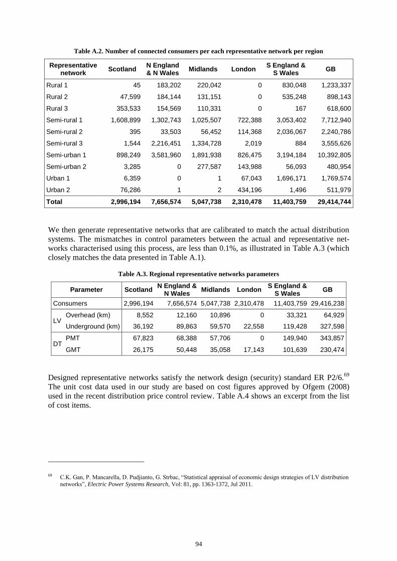
94
Table A.2. Number of connected consumers per each representative network per region
Representative network
Scotland N England & N Wales
Midlands London S England &
S Wales GB
Rural 1 45 183,202 220,042 0 830,048 1,233,337
Rural 2 47,599 184,144 131,151 0 535,248 898,143
Rural 3 353,533 154,569 110,331 0 167 618,600
Semi-rural 1 1,608,899 1,302,743 1,025,507 722,388 3,053,402 7,712,940
Semi-rural 2 395 33,503 56,452 114,368 2,036,067 2,240,786
Semi-rural 3 1,544 2,216,451 1,334,728 2,019 884 3,555,626
Semi-urban 1 898,249 3,581,960 1,891,938 826,475 3,194,184 10,392,805
Semi-urban 2 3,285 0 277,587 143,988 56,093 480,954
Urban 1 6,359 0 1 67,043 1,696,171 1,769,574
Urban 2 76,286 1 2 434,196 1,496 511,979
Total 2,996,194 7,656,574 5,047,738 2,310,478 11,403,759 29,414,744
We then generate representative networks that are calibrated to match the actual distribution
systems. The mismatches in control parameters between the actual and representative net-
works characterised using this process, are less than 0.1%, as illustrated in Table A.3 (which
closely matches the data presented in Table A.1).
Table A.3. Regional representative networks parameters
Parameter Scotland N England &
N Wales Midlands London
S England & S Wales
GB
Consumers 2,996,194 7,656,574 5,047,738 2,310,478 11,403,759 29,416,238
LV Overhead (km) 8,552 12,160 10,896 0 33,321 64,929
Underground (km) 36,192 89,863 59,570 22,558 119,428 327,598
DT PMT 67,823 68,388 57,706 0 149,940 343,857
GMT 26,175 50,448 35,058 17,143 101,639 230,474
Designed representative networks satisfy the network design (security) standard ER P2/6.69
The unit cost data used in our study are based on cost figures approved by Ofgem (2008)
used in the recent distribution price control review. Table A.4 shows an excerpt from the list
of cost items.
69 C.K. Gan, P. Mancarella, D. Pudjianto, G. Strbac, “Statistical appraisal of economic design strategies of LV distribution
networks”, Electric Power Systems Research, Vol: 81, pp. 1363-1372, Jul 2011.

95
Table A.4. Network equipment cost
Asset Units Cost (£k)
LV overhead line km 30.0
LV underground cable km 98.4
11/0.4 kV ground mounted transformer # 13.2
11/0.4 kV pole mounted transformer # 2.9
HV overhead line km 35.0
HV underground cable km 82.9
EHV/11 kV ground mounted transformer # 377.9
A.5. Demand modelling
It is expected that new electricity demand categories such as electrified heating or transport
will play an increasingly important role in decarbonising the electricity sector. We have
gained understanding of specific features of these demand sectors, and have developed de-
tailed bottom-up models which enabled us to produce hourly demand profiles based on large
databases of transport behaviour and building stock data. This allows us to develop detailed
hourly profiles for different demand categories contained in long-term development pathways,
which typically only specify annual energy consumption figures.
Understanding the characteristics of flexible demand and quantifying the flexibility they can
potentially offer to the system is vital to establishing its economic value.70
In order to offer
flexibility, controlled devices (or appliances) must have access to some form of storage when
rescheduling their operation (e.g. thermal, chemical or mechanical energy, or storage of in-
termediate products). Load reduction periods are followed or preceded by load recovery,
which is a function of the type of interrupted process and the type of storage. This in turn re-
quires bottom-up modelling of each individual demand side technology (appliance) under-
standing how it performs its actual function, while exploiting the flexibility that may exist
without compromising the service that it delivers. In our analysis we consider various forms
of domestic and commercial types of flexible demand.71,72,73,74,75, 76,77,78
70 G. Strbac, “Demand side management: Benefits and challenges”, Energy Policy, Vol: 36, pp. 4419-4426, Dec 2008.
71 M. Aunedi, G. Strbac, “Efficient System Integration of Wind Generation through Smart Charging of Electric Vehicles”,
8th International Conference and Exhibition on Ecological Vehicles and Renewable Energies (EVER), Monte Carlo,
March 2013.
72 ENA, SEDG, Imperial College, “Benefits of Advanced Smart Metering for Demand Response based Control of Distri-
bution Networks”, April 2010. Available at:
http://www.energynetworks.org/modx/assets/files/electricity/futures/smart_meters/Smart_Metering_Benerfits_Summar
y_ENASEDGImperial_100409.pdf.
73 C.K. Gan, M. Aunedi, V. Stanojevic, G. Strbac and D. Openshaw: “Investigation of the Impact of Electrifying Trans-
port and Heat Sectors on the UK Distribution Networks”, 21st International Conference on Electricity Distribution (CI-
RED), 6-9 June 2011, Frankfurt, Germany.
74 D. Pudjianto, P. Djapic, M. Aunedi, C. K. Gan, G. Strbac, S. Huang, D. Infield, “Smart control for minimizing distribu-
tion network reinforcement cost due to electrification”, Energy Policy, Vol. 52, pp. 76-84, January 2013.

96
The following assumptions of full DSR flexibility are made in system integration cost stud-
ies:79
Electric vehicles: up to 80% of EV demand could be shifted away from a given hour
to other times of day;
Heat pumps: heat storage enables that the 35% of HP demand can be shifted from a
given hour to other times of day;
Smart appliances: demand attributed to white appliances (washing machines, dish-
washers, tumble dryers) participating in smart operation can be fully shifted away
from peak;
Industrial and commercial demand: 10% of the demand of I&C customers participat-
ing in DSR schemes can be redistributed.
In addition to improving energy management and potentially reducing capacity adequacy re-
quirements due to lower peak demand, these flexible sources are assumed to also be capable
of providing frequency response (maintain grid frequency). It is important to stress that the
magnitude of demand (and therefore the absolute volume of demand that can be shifted) in
each of the above categories changes in time (it is time-specific).
In terms of energy available for shifting in a fully-flexible system, it is assumed the following
demand volumes are movable within day:
EV demand: 15.1 TWh
Heat pump demand: 9.4 TWh
Smart appliance demand: 25.4 TWh
Industrial and commercial loads participating in DSR schemes: 19.0 TWh
75 Imperial College London, “Value of Smart Appliances in System Balancing”, Part I of Deliverable 4.4 of Smart-A pro-
ject (No. EIE/06/185//SI2.447477), September 2009.
76 M. Aunedi, P. A. Kountouriotis, J. E. Ortega Calderon, D. Angeli, G. Strbac, “Economic and Environmental Benefits of
Dynamic Demand in Providing Frequency Regulation”, IEEE Transactions on Smart Grid, vol. 4, pp. 2036-2048, De-
cember 2013.
77 M. Woolf, T. Ustinova, E. Ortega, H. O’Brien, P. Djapic, G. Strbac, “Distributed generation and demand response ser-
vices for the smart distribution network”, Report A7 for the “Low Carbon London” LCNF project: Imperial College
London, 2014.
78 Imperial College and NERA Consulting, 2012, “Understanding the Balancing Challenge”, analysis commissioned by
DECC to support this publication. Please see
https://www.gov.uk/government/uploads/system/uploads/attachment_data/file/48553/5767-understanding-the-
balancing-challenge.pdf
79 An overview of the rationale and evidence behind these assumptions is provided in:
M. Aunedi, F. Teng, G. Strbac, “Carbon impact of smart distribution networks”, Report D6 for the “Low Carbon Lon-
don” LCNF project, December 2014.

97
Note that in our analysis any demand shifting only occurs within the timeframe of one day i.e.
no demand shifting over longer time horizons was considered.


