Workshop report 1. Daniels report is on website 2. Don’t expect to write it based on listening to one project (we had 6 only 2 was sufficient quality) 3. I suggest writing it on one presentation. 4. Include figures (from a related paper or their presentation) 5. Include references Update: We are all set to have your students attend. We will not register them, so they can come and go as needed. food is for the registered participants and please allow them to eat first. Currently we have 70 registered participants and plant to order food for ~100.
i. toobtainanefficient,exactinferencealgorithmforfindingmarginals;ii. insituationswhereseveralmarginalsarerequired,toallowcomputationsto
besharedefficiently.
Keyidea:DistributiveLaw
Efficient inference
7 versus 3 operations
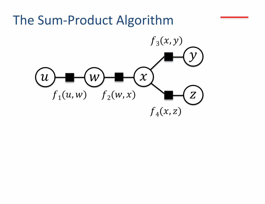
The Sum-Product Algorithm
𝑥 𝑢 𝑤 𝑦
𝑧 𝑓1(𝑢, 𝑤) 𝑓2(𝑤, 𝑥)
𝑓4(𝑥, 𝑧)
𝑓3(𝑥, 𝑦)
KF/PFs offer solutions to dynamical systems, nonlinear in general, using prediction and update as data becomes available. Tracking in time or space offers an ideal framework for studying KF/PF.
How do we solve it and what does the solution look like?
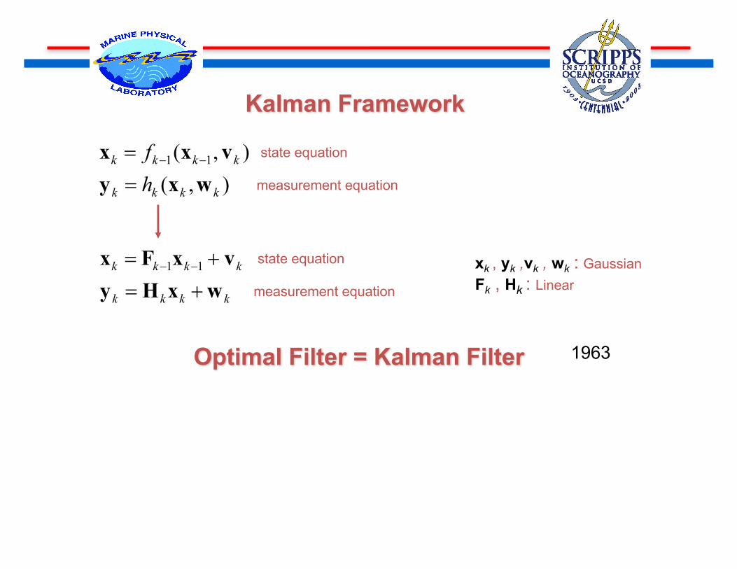
Kalman Framework
kkkk
kkkk
wxHyvxFx
+=+= -- 11 state equation
measurement equation
),(),( 11
kkkk
kkkk
hf
wxyvxx
== -- state equation
measurement equation
xk , yk ,vk , wk : GaussianFk , Hk : Linear
Optimal Filter = Kalman Filter 1963
o
o
o
o
ooo
oo
oo
previous states
xk-1
xk-2
1. Predict the mean using previous history.
2. Predict the covariance using previous history.
3. Correct/update the mean using new data yk
4. Correct/update the covariance using yk
o
),ˆ(~ ||| kkkkkk Pxx N
{ } kkkkkkkk dxxxxxxx ò --- == )|p(|Eˆ 111|
1|ˆ -kkx
1| -kkP
kk |P
o 1|ˆ -kkxkk |x̂
A Single Kalman Iteration
)|p( 1-kk xx
),,|p( 021 xxxx !-- kkk
),,|p( 11 yyyx !-kkk
)|p( kk Yx
{ } kkkkkkkk dxYxxYxx ò== )|p(|Eˆ |
PRED
ICT
UPD
ATE
!! ÞÞÞÞ --- )|p()|p()|p( 111 kkkkkk YxYxYx
PREDICTOR-CORRECTOR DENSITY PROPAGATOR
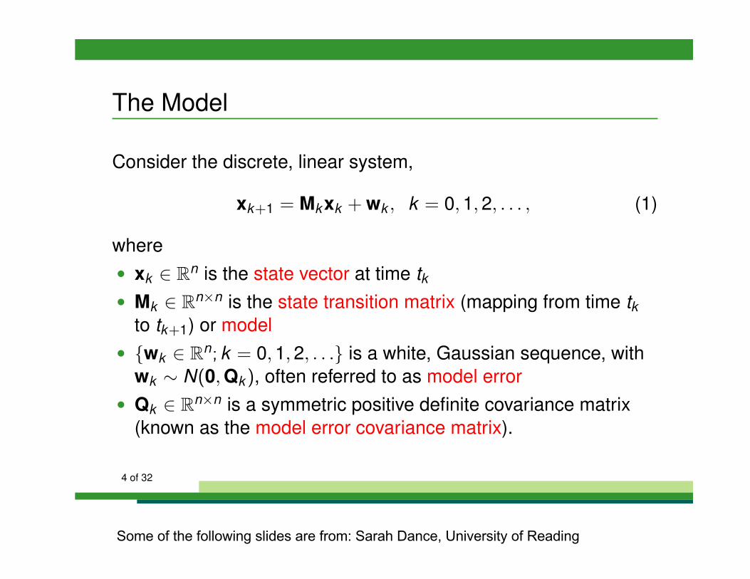
The Model
Consider the discrete, linear system,
xk+1 = Mkxk + wk , k = 0, 1, 2, . . . , (1)
where• xk 2 Rn is the state vector at time tk• Mk 2 Rn⇥n is the state transition matrix (mapping from time tk
to tk+1) or model• {wk 2 Rn; k = 0, 1, 2, . . .} is a white, Gaussian sequence, with
wk ⇠ N(0,Qk ), often referred to as model error• Qk 2 Rn⇥n is a symmetric positive definite covariance matrix
(known as the model error covariance matrix).
4 of 32
Some of the following slides are from: Sarah Dance, University of Reading
The ObservationsWe also have discrete, linear observations that satisfy
yk = Hkxk + vk , k = 1, 2, 3, . . . , (2)
where• yk 2 Rp is the vector of actual measurements or observations
at time tk• Hk 2 Rn⇥p is the observation operator. Note that this is not in
general a square matrix.• {vk 2 Rp; k = 1, 2, . . .} is a white, Gaussian sequence, with
vk ⇠ N(0,Rk ), often referred to as observation error.• Rk 2 Rp⇥p is a symmetric positive definite covariance matrix
(known as the observation error covariance matrix).We assume that the initial state, x0 and the noise vectors at eachstep, {wk}, {vk}, are assumed mutually independent.
5 of 32
The Prediction and Filtering Problems
We suppose that there is some uncertainty in the initial state, i.e.,
x0 ⇠ N(0,P0) (3)
with P0 2 Rn⇥n a symmetric positive definite covariance matrix.
The problem is now to compute an improved estimate of thestochastic variable xk , provided y1, . . . yj have been measured:
bxk |j = bxk |y1,...,yj . (4)
• When j = k this is called the filtered estimate.• When j = k � 1 this is the one-step predicted, or (here) the
predicted estimate.6 of 32
• The Kalman filter (Kalman, 1960) provides estimates for thelinear discrete prediction and filtering problem.
• We will take a minimum variance approach to deriving the filter.• We assume that all the relevant probability densities are
Gaussian so that we can simply consider the mean andcovariance.
• Rigorous justifcation and other approaches to deriving the filterare discussed by Jazwinski (1970), Chapter 7.
8 of 32
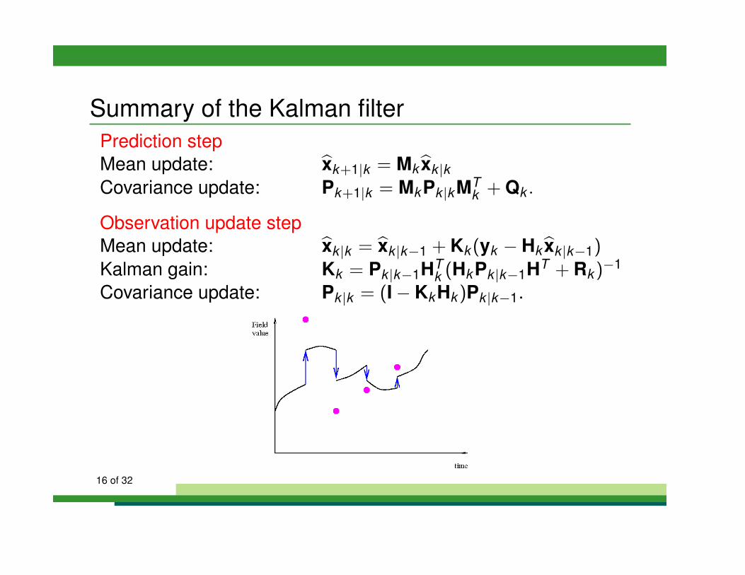
Prediction step
We first derive the equation for one-step prediction of the meanusing the state propagation model (1).
bxk+1|k = E [xk+1|y1, . . . yk ] ,
= E [Mkxk + wk ] ,
= Mkbxk |k (5)
9 of 32
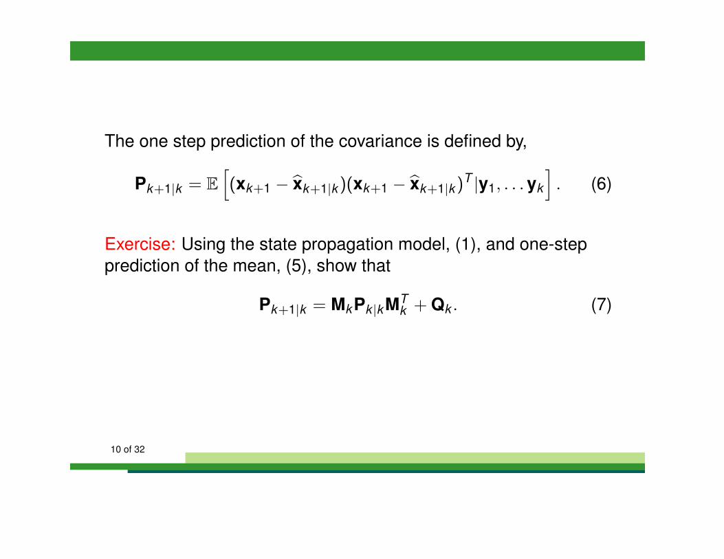
The one step prediction of the covariance is defined by,
Pk+1|k = Eh(xk+1 � bxk+1|k )(xk+1 � bxk+1|k )
T |y1, . . . yk
i. (6)
Exercise: Using the state propagation model, (1), and one-stepprediction of the mean, (5), show that
Pk+1|k = MkPk |kMTk + Qk . (7)
10 of 32
Product(of(Gaussians=Gaussian:(
260
Example: Measuring the mass of an object
p(d|m) � exp½c12(dcGm)TCc1d (dcGm)
¾
� exp½c12[(dcGm)TCc1d (dcGm) + (mcmo)
TCc1m (mcmo)]
¾
The more accurate new data has changed the estimate of m and decreased its uncertainty
For the general linear inverse problem we would have
p(m) � exp½c1
2(mcmo)
TCc1m (mcmo)
¾Prior:
Likelihood:
Posterior PDF
One data point problem
∝ exp −12m− m̂[ ]T S−1 m− m̂[ ]
#$%
&'(
S−1 =GTCd−1G+Cm
−1
m̂ = GTCd−1G+Cm
−1( )−1GTCd
−1d+Cm−1m0( )
= m0 + GTCd
−1G+Cm−1( )
−1GTCd
−1 d−Gm0( )
Filtering Step
At the time of an observation, we assume that the update to themean may be written as a linear combination of the observationand the previous estimate:
bxk |k = bxk |k�1 + Kk (yk � Hkbxk |k�1), (8)
where Kk 2 Rn⇥p is known as the Kalman gain and will be derivedshortly.
11 of 32
But first we consider the covariance associated with this estimate:
Pk |k = Eh(xk � bxk |k )(xk � bxk |k )
T |y1, . . . yk
i. (9)
Using the observation update for the mean (8) we have,