

Workshopreport1. Danielsreportisonwebsite2. Don’texpecttowriteitbasedonlisteningtooneproject(wehad6
only2wassufficientquality)3. Isuggestwritingitononepresentation.4. Includefigures(fromarelatedpaperortheirpresentation)5. Includereferences
Update:Weareallsettohaveyourstudentsattend.Wewillnotregisterthem,sotheycancomeandgoasneeded. foodisfortheregisteredparticipantsandpleaseallowthemtoeatfirst.Currentlywehave70registeredparticipantsandplanttoorderfoodfor~100.

May22,Dictionarylearning,MikeBianco(halfclass),BishopCh 13May24,ClassHWBishopCh 8/13MAY30CODYMay31,NoClass.Workshop, BigDataandTheEarthSciences:GrandChallengesWorkshopJune5,Discussworkshop,Discussfinalproject.Spiess Hallopenforprojectdiscussion11am-7pm.June7,Workshopreport.NoclassJune12Spiess Hallopenforprojectdiscussion9-11:30amand2-7pmJune16Finalreportdelivered.Beertime
Forfinalprojectdiscussionevery afternoonMarkandIwillbeavailable
InclassonJuly5astatusreportfromeachgroupismandatory.Maximum2min/person,(i.e.a5-membergrouphave10min),shorterisfine.HavepresentationonmemorystickoremailMark.Classmightrunlonger,sowecouldstartearlier.FortheFinalproject(Due16June5Pm).DeliveryDropboxrequest<2GB(detailstofollow).:
A) Deliveracode:1) Assumewehavereasonablecompilersinstalled(weuseMacOsX)2) Giveinstructionsifanyadditionalsoftwareshouldbeinstalled.3) Youcanaskustodownloadadataset.Orincludeitinthissubmission4) Don’tincludealldevelopedcodes.Justkeyelements.5) Weshouldnothavetoreprogramyourcode.
B) Report1) Thereportshouldincludeallthefollowingsections:Summary->Introduction->Physicaland
Mathematicalframework->Results.2) Summaryisacombinationofanabstractandconclusion.3) Plagiarismisnotacceptable!Whencitinguse““forquotesandcitationsforrelevant
papers.4) Don’twriteanythingyoudon’tunderstand.5) Everyoneinthegroupshouldunderstandeverythingthatiswritten.Ifwedonot
understandasectionduringgradingweshouldbeabletoaskanymemberofthegrouptoclarify.Youcandelegatethewriting,butnottheunderstanding.
6) Usecitations.Anyconceptswhicharenotfullyexplainedshouldhaveacitationwithanexplanation.
7) Pleasebeconcise.Equationsaregood.Figuresessential.Writeasthoughyourreportistobepublishedinascientificjournal.
8) IhaveattachedasamplereportfromMark,thoughshorterispreferred.
FinalReport
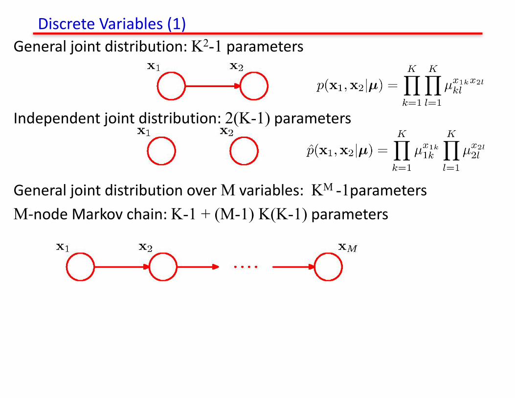
DiscreteVariables(1)Generaljointdistribution:K2-1 parameters
Independentjointdistribution:2(K-1) parameters
GeneraljointdistributionoverM variables:KM -1parametersM-nodeMarkovchain:K-1 + (M-1) K(K-1) parameters
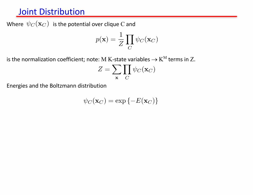
JointDistributionWhereisthepotentialovercliqueC and
isthenormalizationcoefficient;note:M K-statevariables® KM termsinZ.
EnergiesandtheBoltzmanndistribution

Illustration:ImageDe-Noising
NoisyImage RestoredImage(ICM) RestoredImage(Graphcuts)

InferenceinGraphicalModels

InferenceonaChain

InferenceonaChain

InferenceonaChain
Tocomputelocalmarginals:• Computeandstoreallforwardmessages,.• Computeandstoreallbackwardmessages,.• ComputeZ atanynodexm
• Compute
forallvariablesrequired.

TheSum-ProductAlgorithm(1)Objective:
i. toobtainanefficient,exactinferencealgorithmforfindingmarginals;ii. insituationswhereseveralmarginalsarerequired,toallowcomputationsto
besharedefficiently.
Keyidea:DistributiveLaw
Efficient inference
7 versus 3 operations
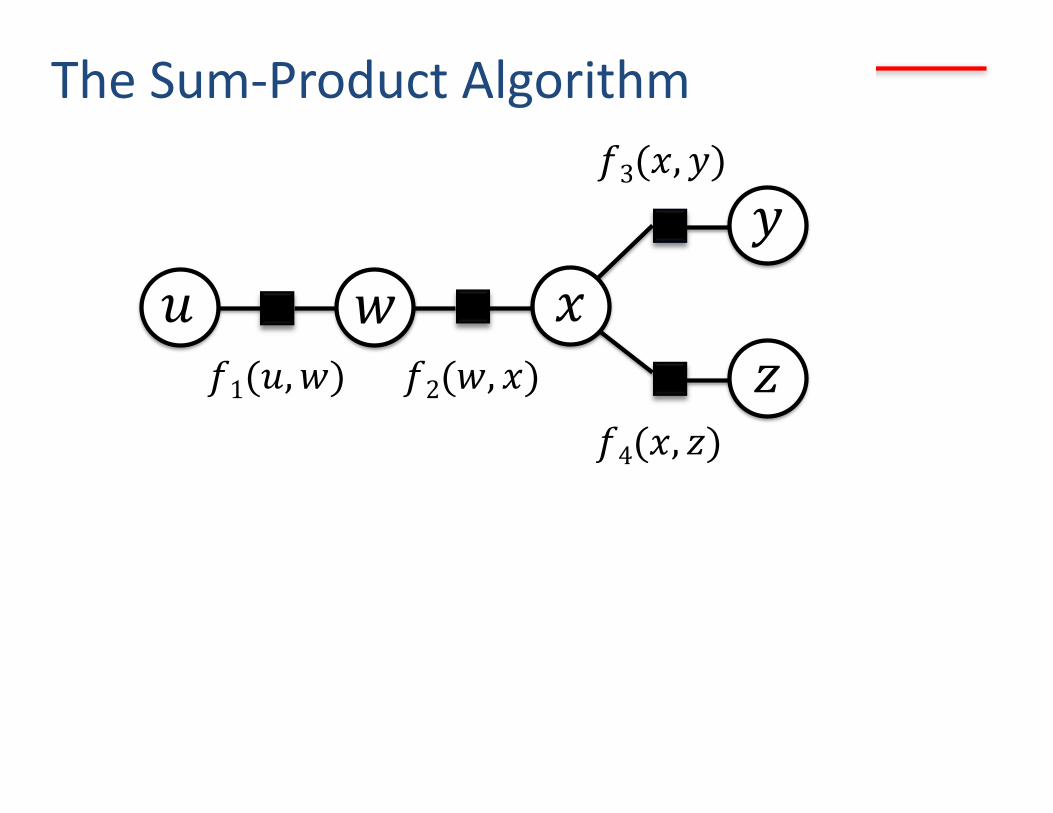
The Sum-Product Algorithm
𝑥 𝑢 𝑤 𝑦
𝑧 𝑓1(𝑢, 𝑤) 𝑓2(𝑤, 𝑥)
𝑓4(𝑥, 𝑧)
𝑓3(𝑥, 𝑦)

KF/PFs offer solutions to dynamical systems, nonlinear in general, using prediction and update as data becomes available. Tracking in time or space offers an ideal framework for studying KF/PF.
How do we solve it and what does the solution look like?
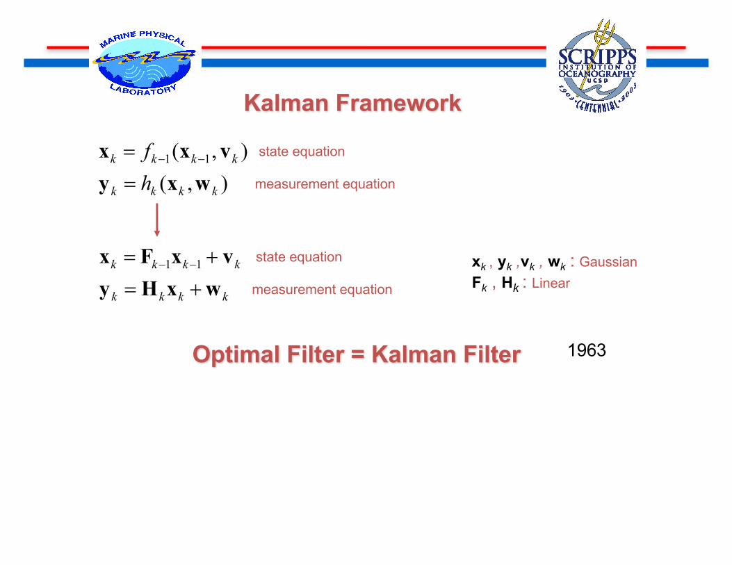
Kalman Framework
kkkk
kkkk
wxHyvxFx
+=+= -- 11 state equation
measurement equation
),(),( 11
kkkk
kkkk
hf
wxyvxx
== -- state equation
measurement equation
xk , yk ,vk , wk : GaussianFk , Hk : Linear
Optimal Filter = Kalman Filter 1963

o
o
o
o
ooo
oo
oo
previous states
xk-1
xk-2
1. Predict the mean using previous history.
2. Predict the covariance using previous history.
3. Correct/update the mean using new data yk
4. Correct/update the covariance using yk
o
),ˆ(~ ||| kkkkkk Pxx N
{ } kkkkkkkk dxxxxxxx ò --- == )|p(|Eˆ 111|
1|ˆ -kkx
1| -kkP
kk |P
o 1|ˆ -kkxkk |x̂
A Single Kalman Iteration
)|p( 1-kk xx
),,|p( 021 xxxx !-- kkk
),,|p( 11 yyyx !-kkk
)|p( kk Yx
{ } kkkkkkkk dxYxxYxx ò== )|p(|Eˆ |
PRED
ICT
UPD
ATE
!! ÞÞÞÞ --- )|p()|p()|p( 111 kkkkkk YxYxYx
PREDICTOR-CORRECTOR DENSITY PROPAGATOR
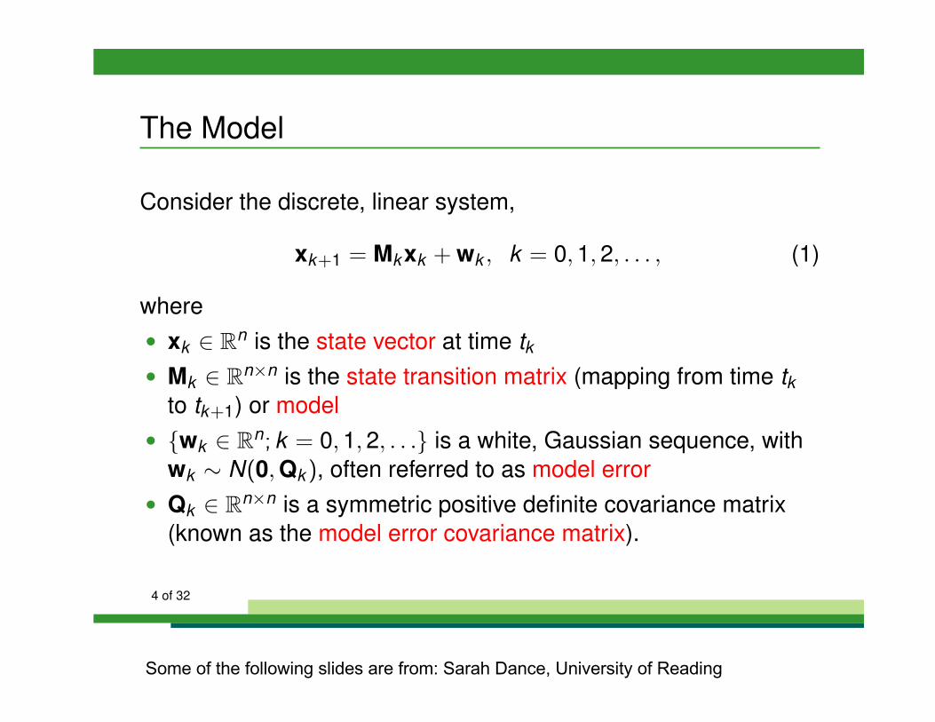
The Model
Consider the discrete, linear system,
xk+1 = Mkxk + wk , k = 0, 1, 2, . . . , (1)
where• xk 2 Rn is the state vector at time tk• Mk 2 Rn⇥n is the state transition matrix (mapping from time tk
to tk+1) or model• {wk 2 Rn; k = 0, 1, 2, . . .} is a white, Gaussian sequence, with
wk ⇠ N(0,Qk ), often referred to as model error• Qk 2 Rn⇥n is a symmetric positive definite covariance matrix
(known as the model error covariance matrix).
4 of 32
Some of the following slides are from: Sarah Dance, University of Reading

The ObservationsWe also have discrete, linear observations that satisfy
yk = Hkxk + vk , k = 1, 2, 3, . . . , (2)
where• yk 2 Rp is the vector of actual measurements or observations
at time tk• Hk 2 Rn⇥p is the observation operator. Note that this is not in
general a square matrix.• {vk 2 Rp; k = 1, 2, . . .} is a white, Gaussian sequence, with
vk ⇠ N(0,Rk ), often referred to as observation error.• Rk 2 Rp⇥p is a symmetric positive definite covariance matrix
(known as the observation error covariance matrix).We assume that the initial state, x0 and the noise vectors at eachstep, {wk}, {vk}, are assumed mutually independent.
5 of 32

The Prediction and Filtering Problems
We suppose that there is some uncertainty in the initial state, i.e.,
x0 ⇠ N(0,P0) (3)
with P0 2 Rn⇥n a symmetric positive definite covariance matrix.
The problem is now to compute an improved estimate of thestochastic variable xk , provided y1, . . . yj have been measured:
bxk |j = bxk |y1,...,yj . (4)
• When j = k this is called the filtered estimate.• When j = k � 1 this is the one-step predicted, or (here) the
predicted estimate.6 of 32

• The Kalman filter (Kalman, 1960) provides estimates for thelinear discrete prediction and filtering problem.
• We will take a minimum variance approach to deriving the filter.• We assume that all the relevant probability densities are
Gaussian so that we can simply consider the mean andcovariance.
• Rigorous justifcation and other approaches to deriving the filterare discussed by Jazwinski (1970), Chapter 7.
8 of 32

Prediction step
We first derive the equation for one-step prediction of the meanusing the state propagation model (1).
bxk+1|k = E [xk+1|y1, . . . yk ] ,
= E [Mkxk + wk ] ,
= Mkbxk |k (5)
9 of 32
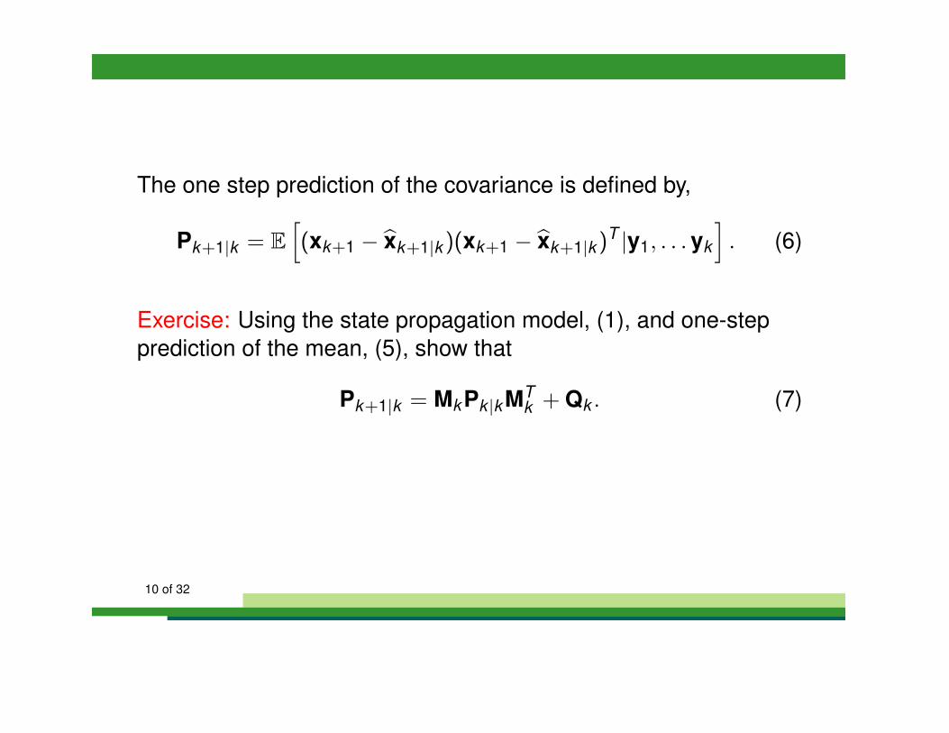
The one step prediction of the covariance is defined by,
Pk+1|k = Eh(xk+1 � bxk+1|k )(xk+1 � bxk+1|k )
T |y1, . . . yk
i. (6)
Exercise: Using the state propagation model, (1), and one-stepprediction of the mean, (5), show that
Pk+1|k = MkPk |kMTk + Qk . (7)
10 of 32

Product(of(Gaussians=Gaussian:(
260
Example: Measuring the mass of an object
p(d|m) � exp½c12(dcGm)TCc1d (dcGm)
¾
� exp½c12[(dcGm)TCc1d (dcGm) + (mcmo)
TCc1m (mcmo)]
¾
The more accurate new data has changed the estimate of m and decreased its uncertainty
For the general linear inverse problem we would have
p(m) � exp½c1
2(mcmo)
TCc1m (mcmo)
¾Prior:
Likelihood:
Posterior PDF
One data point problem
∝ exp −12m− m̂[ ]T S−1 m− m̂[ ]
#$%
&'(
S−1 =GTCd−1G+Cm
−1
m̂ = GTCd−1G+Cm
−1( )−1GTCd
−1d+Cm−1m0( )
= m0 + GTCd
−1G+Cm−1( )
−1GTCd
−1 d−Gm0( )

Filtering Step
At the time of an observation, we assume that the update to themean may be written as a linear combination of the observationand the previous estimate:
bxk |k = bxk |k�1 + Kk (yk � Hkbxk |k�1), (8)
where Kk 2 Rn⇥p is known as the Kalman gain and will be derivedshortly.
11 of 32

But first we consider the covariance associated with this estimate:
Pk |k = Eh(xk � bxk |k )(xk � bxk |k )
T |y1, . . . yk
i. (9)
Using the observation update for the mean (8) we have,
xk � bxk |k = xk � bxk |k�1 � Kk (yk � Hkbxk |k�1)
= xk � bxk |k�1 � Kk (Hkxk + vk � Hkbxk |k�1),
replacing the observations with their model equivalent,= (I � KkHk )(xk � bxk |k�1)� Kkvk . (10)
Thus, since the error in the prior estimate, xk � bxk |k�1 isuncorrelated with the measurement noise we find
Pk |k = (I � KkHk )Eh(xk � bxk |k�1)(xk � bxk |k�1)
Ti(I � KkHk )
T
+KkEhvkvT
k
iKT
k . (11)
12 of 32

Simplification of the a posteriori error covarianceformula
Using this value of the Kalman gain we are in a position to simplifythe Joseph form as
Pk |k = (I�KkHk )Pk |k�1(I�KkHk )T +KkRkKT
k = (I�KkHk )Pk |k�1.(15)
Exercise: Show this.
Note that the covariance update equation is independent of theactual measurements: so Pk |k could be computed in advance.
15 of 32
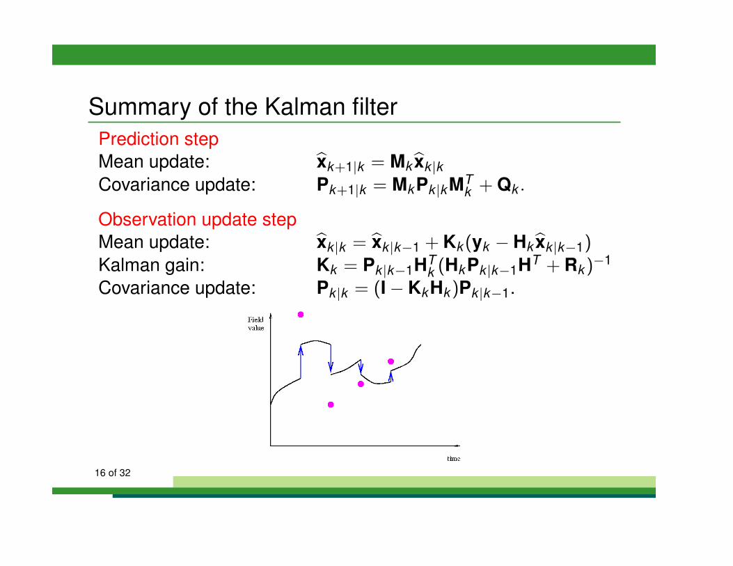
Summary of the Kalman filterPrediction stepMean update: bxk+1|k = Mkbxk |kCovariance update: Pk+1|k = MkPk |kMT
k + Qk .
Observation update stepMean update: bxk |k = bxk |k�1 + Kk (yk � Hkbxk |k�1)Kalman gain: Kk = Pk |k�1HT
k (HkPk |k�1HT + Rk )�1
Covariance update: Pk |k = (I � KkHk )Pk |k�1.
16 of 32


