1 THE GROWTH OF WORLD AGRICULTURAL PRODUCTION, 1800-1938 Giovanni Federico Running Head: World Agricultural Production JEL Codes: N5, Q1, O4 Keywords: agriculture, output, world Mailing address: Professor Giovanni Federico Department of History and Civilization European University Institute Via Boccaccio 121 I-50133 Firenze. ITALY E-mail: [email protected]Telephone: +390554685548 Fax: +390554685203
Transcript
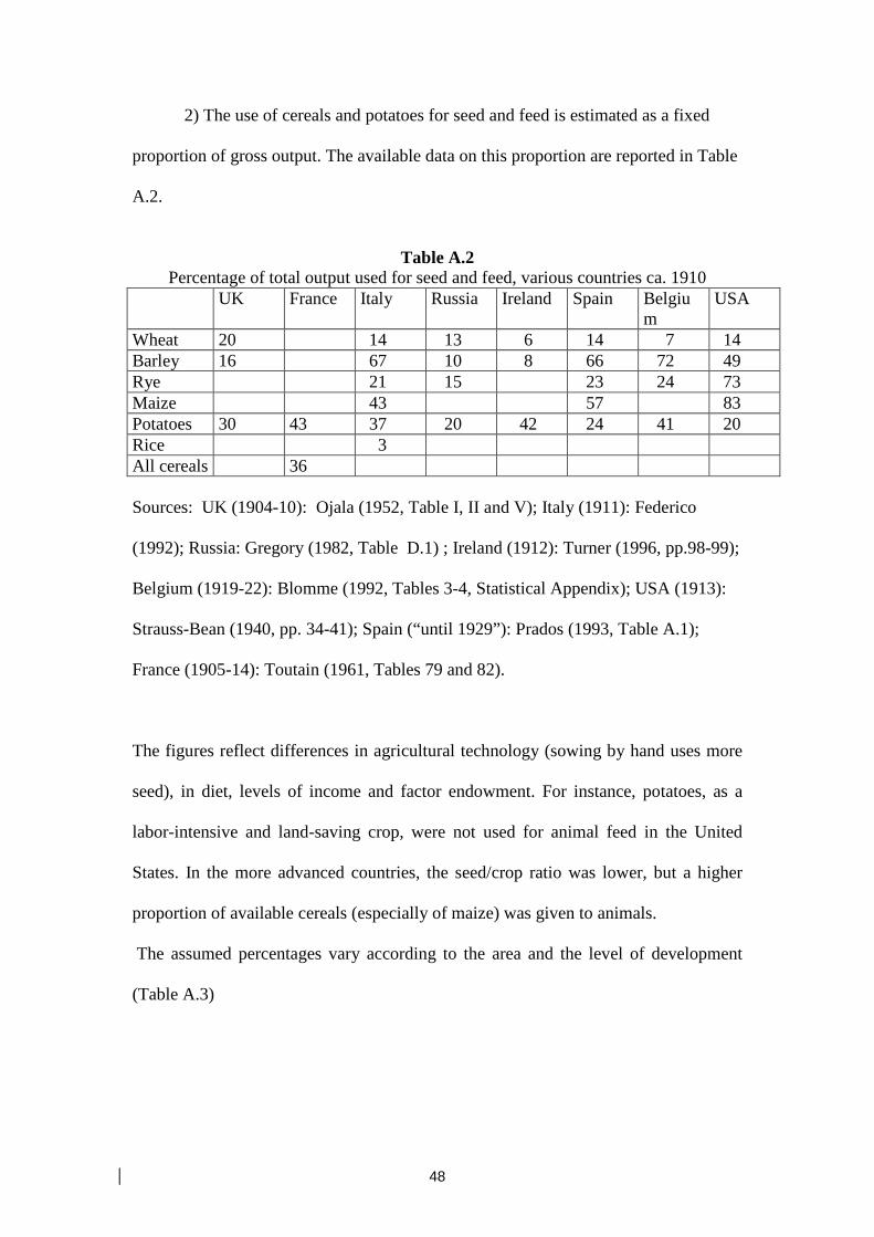
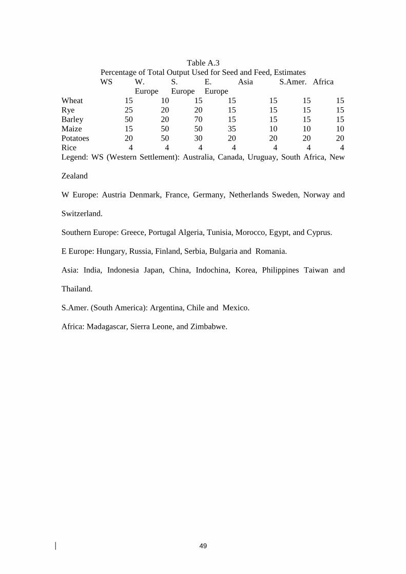
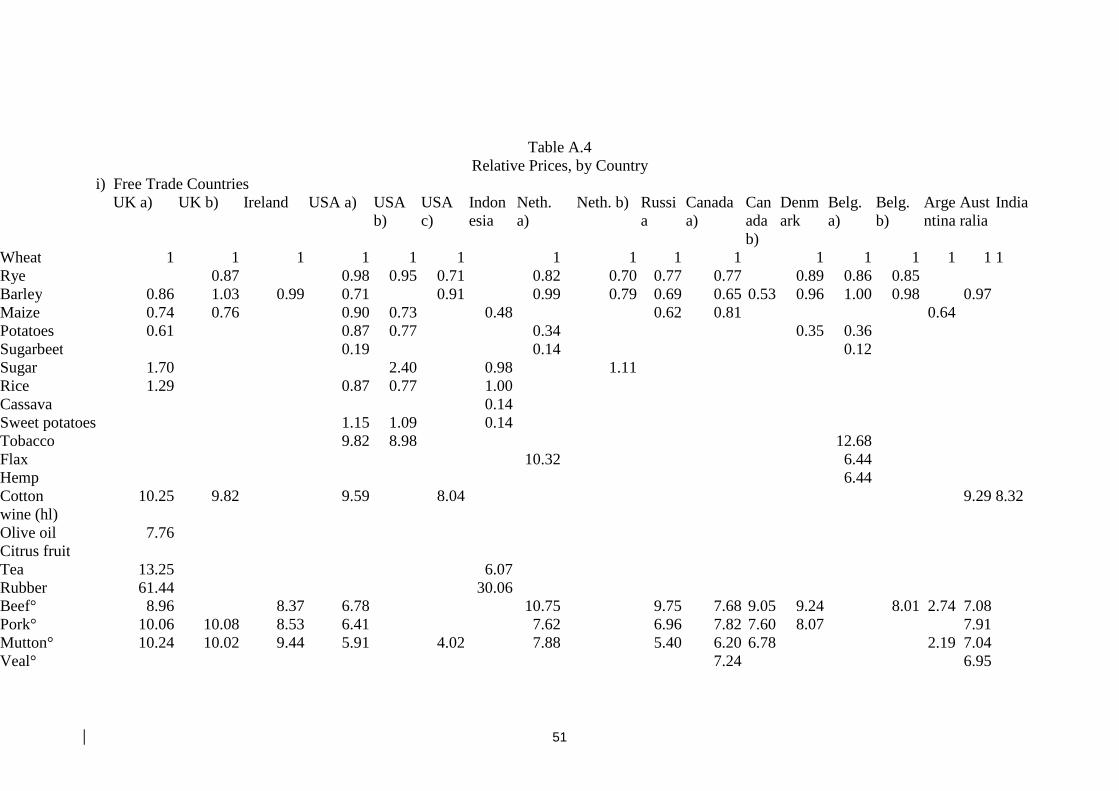
1
THE GROWTH OF WORLD AGRICULTURAL PRODUCTION, 1800-1 938
Giovanni Federico
Running Head: World Agricultural Production
JEL Codes: N5, Q1, O4
Keywords: agriculture, output, world
Mailing address:
Professor Giovanni Federico
Department of History and Civilization European University Institute Via Boccaccio 121 I-50133 Firenze. ITALY
World population has increased six-fold in the last two centuries, and thus
agricultural production must have grown as well. The last fifty years of this
increase are covered by the Food and Agriculture Organization (FAO) production
series. This article aims to push our quantitative knowledge back in time as far as
possible. It reviews the scattered evidence on agricultural production in the first
half of the 19th century, estimates a yearly series of output for the main countries
since 1870, and puts forward some guesstimates on trends in the rest of the world.
In the long run, agricultural production has increased more than population.
Growth has affected all continents, even if it has been decidedly faster in both the
countries of Western Settlement and in Eastern Europe, than in Asia or in Western
Europe. It was faster before World War One, a veritable golden age for world
agriculture, than in the inter-war years. The composition of production has
changed as well, with an increase in the share of livestock products.
3
I. INTRODUCTION: WHY SHOULD WE CARE ABOUT
AGRICULTURE?
D. Gale Johnson reminded the audience in his 1999 Presidential
Address to the American Economic Association that “people today have
more adequate nutrition than ever before and have acquired that nutrition
at the lowest cost in all human history, while the world has more people
than ever before – not by a little but by a lot” (Johnson, 2000, p. 1).
Nowadays, world population exceeds six billion people and, in theory,
each of them could consume 2800 calories per day – a more than adequate
intake.1 This average conceals wide disparities among the continents and
malnutrition is still widespread, especially in Sub-Saharan Africa, where
the official average daily availability is about 2200 calories. However, true
starvation is rare, and is almost always caused by wars and political
events, which disrupt agriculture and trade in agricultural products, and
make food relief efforts too dangerous.
Two hundred years ago, world population was a mere one billion,
and its average caloric consumption was undoubtedly lower – possibly as
low as 1800 calories in France or 2200 in the United Kingdom, the two
most advanced countries in Europe.2 Throughout the world, there was a
real risk of starvation, especially for poor and destitute people, and terrible
famines hit several countries in the 19th century (e.g., Ireland, Finland,
India, and so on). Thus, there must have been a hug increase in world
agricultural production. Indeed, according to the latest FAO estimates,
4
world gross output increased by 60 percent from 1938 to the late 1950s,
and more than doubled from then to 2001.3
Output must also have increased in the previous one hundred and
fifty years, but the extent of this growth is still poorly known. Before
1870, the statistical evidence is scarce. Historians have tried to deduce the
performance of agriculture from that of the overall economy: agricultural
production is assumed to have grown fast in the early starters (notably, the
United Kingdom, but also the United States), and to have remained
stagnant in the late-comers, such as Italy or Russia. The evidence on the
period after 1870 is more abundant, but it does not seem to attract much
attention among historians. For instance, agriculture is barely mentioned
in popular textbooks on 19th and 20th century modern economic growth,
such as those by Rosenberg-Birdzell (1986), Cameron (1989) and Landes
(1998).
Agriculture does not directly feature in the recent literature on 19th
century globalization (Williamson-O’Rourke, 1999) either. Their general
framework, however with its strong stress on factor endowments and
migration flows, implies different rates of growth in agricultural
production comparing the New World (North America, South America
and Oceania) with the Old World (Europe). The combination of abundant
land and immigrant labor must have caused production to grow faster in
the countries of Western Settlement than in Europe, where the land
endowment was roughly constant, and the labor force was not increasing
fast. The fall in freight rates made it possible to feed Europeans with the
production of Western Settlement countries. Agriculture regains a central
5
(and negative) role in interpretations of economic trends after the Great
War. In fact, overproduction in the 1920s and the fall in agricultural prices
are routinely listed among the causes of the Great Crisis.4
One can sum up the conventional wisdom in five stylized facts: 1)
agricultural production grew in the long run, at least as much as
population and probably more; 2) this growth was slow in the first half of
the 19th century, accelerated in the second half of the century and at the
beginning of the 20th, only to slow down again after World War One; 3)
the growth was faster in Western Settlement countries than in the long-
settled areas of Europe and Asia, where it was faster in the “advanced”
countries than in the “peripheries”; 4) before 1913, the integration of
world markets caused prices to converge, so that prices rose in land-
abundant exporting countries and fell in land-scarce European countries
(when not artificially propped up by duties); 5) prices in the 1920s and
1930s were low and not profitable.
This article aims to test these statements, focusing on the first three.5
After a brief methodological discussion in section two, section three
reviews the evidence on agricultural growth, mainly in Europe, during the
first seventy years of the 19th century. Section four deals with the period
from 1870 to 1938, on the basis of a new series of “world” production,
which covers the whole of Europe (except for Norway and some Balkan
countries), North America and Oceania, and substantial parts of Asia and
South America.6 Section five discusses the reliability of this series and the
possible biases from errors in the country data or in the aggregation
procedure. Section six presents the available evidence on production
6
trends in other countries (including China), while section seven puts
forward some guesstimates about total world output. Finally, section eight
deals with the change in the composition of agricultural production.
Section nine concludes.
II. SOURCES AND METHODS
Agricultural production can be measured either by gross saleable
production or GSP (often referred to as “gross output” or “final product”)
or by Value Added (or GDP).7 The former is defined as the total market
value of all products, net of re-uses within agriculture itself of seed and
feed, but inclusive of farmers’ domestic consumption, while Value Added
is the GSP net of the cost of inputs purchased from outside the sector. It is
worthwhile computing both series, as they measure two different aspects
of agricultural performance. The gross output measures the capability of
agriculture to provide food, clothing, and heating, while Value Added
measures its capability to create income. Furthermore, the ratio of Value
Added to Gross output is a simple proxy for the diffusion of “modern”
agricultural techniques which require the purchase of industrial output
(fertilizers, fuel, industrial feedstuffs, etc.). It is likely to have declined in
the long run – a sixth stylized fact to test.
In recent years, economic historians have worked hard to estimate
national accounts and series of agricultural production. It has been
possible to find yearly series for twenty-five countries (at their 1913
boundaries). In some cases, the source provides both Gross Output and
Value Added, in others only one series. Some of these series extend back
7
in time to the first half of the 19th century (as early as 1800 for Sweden),
while the majority start in the 1850s or 1860s, and five start after 1870.
The series for some key European countries (Russia, Germany, France,
etc.) do not cover the war-time years because during the period of
hostilities these countries ceased to publish statistics. With some plausible
guesswork, it has been possible to build twin series of Gross Output and
Value Added for all twenty-five countries from 1870 to 1913 and from
1920 to 1938.8 They refer to agriculture only, not to the primary sector as
a whole, as the data on production in forestry, fishing and hunting are not
available for some key countries, such as the United States, France, and
the United Kingdom. However, the differences between agriculture and
the primary sector are very small: the omitted activities account for more
than a tenth of the production of the primary sector only in Sweden and
Finland.9
“World” indices of Gross Output and Value Added are obtained by
weighting the country series with their respective shares of production in
1913. This year has been chosen for sound historical reasons (it marks the
end of a long period of expansion of the world economy) and for more
mundane ones. It seems advisable to select a late date, because the
accuracy of the data tends to increase through time, but the choice of any
post-war date (e.g., 1938) would amplify the effect of any error in
boundary adjustments. The value of production in 1913, measured by
sources in national currencies, is converted into British pounds at the
market exchange rates.10
8
III. THE GROWTH OF AGRICULTURAL PRODUCTION IN
THE FIRST HALF OF THE 19TH CENTURY
The statistical evidence on agricultural production in the first half of
the 19th century (Table 1) is incomplete and, in all likelihood, less accurate
and reliable than for later periods.
TABLE 1 ABOUT HERE
The results tally only partially with the conventional wisdom. First,
the performance is better than often assumed. Total production rose in all
countries except Portugal, and, in nine cases out of fifteen, it grew
substantially faster than population.11 Second, the country ranking differs
quite markedly from a priori expectations. The most striking result is the
boom in Egypt, which, however, as warned by Hansen and Whattleworth
(1978, p. 458), seems too good to be true. At the other end of the range,
the fall in production per capita in England, is also striking. It contrasts not
only with the country’s reputation as a beacon for technical progress, but
also with the likely increase in consumption per capita during the
Industrial revolution, when imports of agricultural products were
negligible. There is no easy solution to this “food puzzle” (Clark-
Huberman-Lindert, 1995) but the fact that production growth was not
impressive seems now well-established.
As expected, production grew very fast in the countries of Western
Settlement (a 3 percent increase over 70 years corresponds to an eight-fold
growth). However, the achievement is less impressive than it might seem:
the increase barely exceeded population growth, both in Australia and in
9
the United States.12 In contrast, according to these estimates, European
performance was surprisingly good. Production per capita increased in all
countries, except Austria and Portugal, and, in some cases, quite fast – up
to 0.7 percent per year. Scattered evidence points to an increase in output
also in other countries, such as Austria before 1830, Hungary, and
Russia.13 However, the relative prices of agricultural products rose quite
substantially, especially during the “hungry Forties”, and heights, which,
ceteris paribus depend on food consumption, were falling or stagnant in
the first half of the century in the United States and in several European
countries.14 These facts cast some doubt on the reliability of the figures in
Table 1, which should be considered an upper bound on the true rate of
growth.
The world outside the “Atlantic economy” (with the exception of
Java) is, statistically speaking, terra incognita. Maddison opines that, in
Togukawa Japan, agricultural production grew a bit faster than the
population – i.e. by 20 percent from 1820 to 1870.15 In China, production
may have grown slightly less than population, which rose from about 340
million in 1800, to 410 in 1840, to plunge to 360 million in 1870 because
of the Tai’ping rebellion.16 The total population of the Third World
countries, including China, increased at about 0.3-0.4 percent yearly in the
first half of the 19th century – i.e., by a quarter or by a third (the data are
extremely uncertain).17
If production had been stagnant, consumption per capita would have
fallen by the same amount. Such a fall is unlikely. Caloric consumption at
the beginning of the century was quite low – perhaps less than 2000
10
calories per day per capita in Asian countries, such as Japan and Java (Van
Zanden, 2003). Furthermore, in most countries, land was still quite
abundant, and thus there was ample scope for production growth even
without technical progress. In other words, the best, or least bad, guess,
suggests that agricultural production in the LDCs must have risen,
possibly as much as their population. As said previously, production per
capita in “advanced” countries was rising. Thus, one can, very tentatively,
conclude that, in the first seventy years of the 19th century, world output
per capita did not fall and may have increased.
IV. LONG-TERM GROWTH AND POLITICAL SHOCKS, 1870
TO 1938
The yearly series confirm the conventional wisdom about long-term
growth.18 From 1870 to 1938, “world” gross output increased by 2.5 times
(1.31 percent yearly) and “world” GDP by 2.2 times, at 1.18 percent per
annum (Graph 1). As expected, the growth was faster before 1913 than
afterwards, and there is some (weak) evidence of a slowdown during the
so-called Great Depression.19
GRAPH 1 ABOUT HERE
The data also confirm the received wisdom about the effects of
modernization of agriculture. Purchases outside the sector absorbed 8.5
percent of total GSP in the 1870s, 11 percent on the eve of World War
One and, after a fall caused by the war itself, more than 15 percent in the
late 1930s. Most of these sums were spent to purchase fertilizers, as the
use of tractors and other machinery was to spread massively only after
11
World War Two (Federico, forthcoming). Thus, this statistical
reconstruction by and large buttresses the conventional wisdom. However,
there are also substantial divergences in long-term trends by country/area
performance (Table 2) and in short-term changes during the interwar
period
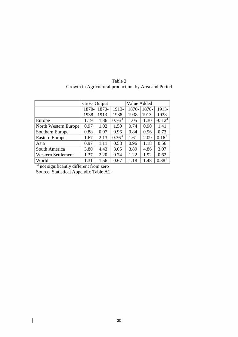
TABLE 2 ABOUT HERE
GRAPH 2 ABOUT HERE
GRAPH 3 ABOUT HERE
Before 1913, the growth in agricultural output was slower than
expected in the countries of Western Settlement (with the remarkable
exception of Argentina) and faster in Eastern Europe. Agricultural
production in the rest of Europe and in Asia grew as well, even though
less than in the countries of Western Settlement or in Russia. However,
performance widely differed between countries in the same area. The area-
wide rates of change conceal remarkable differences by country
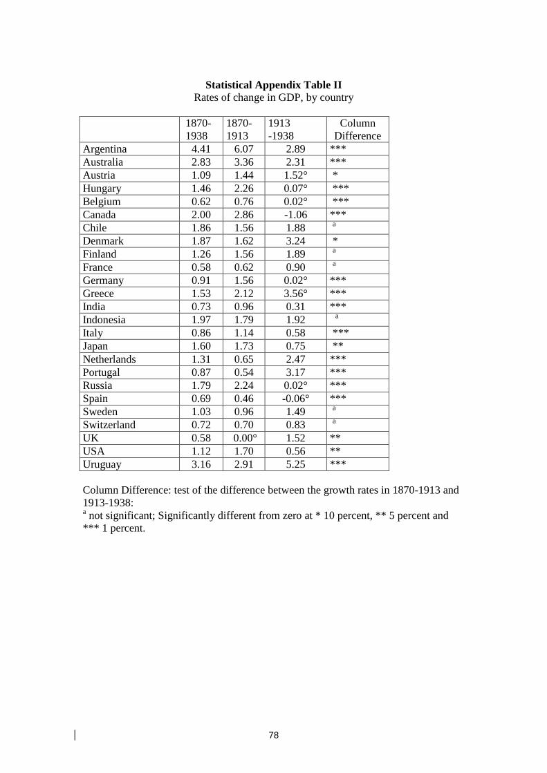
(Statistical Appendix Table II ). India dragged down the otherwise high
growth rate of Indonesia and Japan. In Northwestern Europe, the good
performance of Germany and Denmark contrasts with the lackluster
growth in France, the Netherlands and Belgium, and the stagnation in the
United Kingdom. Greece outshone the two other Mediterranean countries,
with a growth rate that was twice that of Italy and 4.5 times that of Spain.
These differences reflect different combinations of growth in inputs
(extensive growth) and in their productivity (intensive growth). At one end
of the range, Argentina was the prototype of extensive growth, featuring
an exceedingly fast population growth, an almost infinite supply of land
12
and, at least in the 1900s, declining productivity.20 In some European
countries, such as France, Ireland, and the United Kingdom, Total Factor
Productivity grew more than output, and the quantity of inputs (especially
labor) declined.21 All other countries fall somewhere between these
extremes. For instance, in the United States, from 1870 to 1900 inputs
roughly doubled, while output increased by 135 percent: Total Factor
Productivity thus accounted for about a fifth of production growth (Craig-
Weiss, 2000).
The period to 1913 not only shows a growth in production, but also
quite favorable price trends. At the very least, the real prices of
agricultural products remained constant or rose, as in the United States,
while the terms of trade (relative to manufacturers only) increased in
almost all countries. As expected, there is some evidence of price
convergence between the land-abundant New World and the land-scarce
Old World, but it is quite weak. In fact, the range of country cases is quite
wide. However, this combination of growing production and (probably)
rising prices singles out the period to 1913 as a golden age for agriculture,
at least in the Atlantic economy.
The outbreak of the war changed the situation. As already said, it is
impossible to calculate the “world” indices during war-time years, but it is
possible to compute series for some areas (Table 3), and there are
independent estimates of production (especially of cereals) for almost all
the missing countries. Assuming that these estimates are reliable enough,
and that cereal output is a good proxy for the whole of agricultural
13
production, it is possible to estimate that the “world” gross output in 1915-
18 was about 8 percent lower than in 1913.22
TABLE 3 ABOUT HERE
This overall decline is the outcome of widely different country
trends. Asia was relatively unaffected by war, and, in fact, in 1915-1918,
its production continued to rise exactly at the pre-war rate. Production
stagnated in neutral European countries and in overseas countries. The
increase in freights and the embargo on Germany disrupted their
traditional exports flows, even though cereals were no longer subject to
Russian and Romanian competition after the closure of the Dardanelles. In
all the belligerent European countries production fell. The mobilization
drained men and horses from the fields and the conversion of chemical
plants to the production of explosives drastically curtailed the supply of
fertilizers. This shortage may account for the poorer performance in
“modern” countries, such as France or Germany, as compared with Italy
or Russia.
The post-war recovery was decidedly slow. In 1920-22, “world”
output was still about 8-9 percent below the pre-war level.23 Actually,
production exceeded the 1913 level in the majority of countries, including
the United States, but “world” recovery was hampered by failure in three
major countries, Austria-Hungary, Germany, and Russia, which accounted
for about a quarter of “world” output in 1913. In the former Central
Empires, production stagnated around its war-time level, while in Russia,
in 1920-21, while the civil war was raging, it collapsed to (perhaps) half
the pre-war level. As late as 1927-29, “world” production was only 10
14
percent higher than in 1913, and European production was only 5 percent
higher.
Thus, looking at aggregate production figures, there is little evidence
of the alleged overproduction in the 1920s. In-fact, the growth in “world”
production barely matched the increase in population (from 1913 to 1930,
by 11 percent in the world, and by 13 percent in the 25 countries). Nor did
trends in prices confirm the conventional wisdom. Indeed, prices fell in
the early 1920s, but, in most countries, they returned quite quickly to their
pre-war peaks (and, in a handful of countries, terms of trade actually
exceeded the 1913 level). During the Great Depression, prices fell
drastically (by 25-30 percent in most countries), while production
remained constant. The three-year moving averages (a rough measure to
smooth the effect of crop fluctuations) only decreased in 1931, by less
than 1 percent, which was exclusively because of the collectivization
disaster in the Soviet Union.24 On the eve of World War Two, “world”
production was 3-5 percent higher than in 1927-29. Gross output grew
even more (by 8-9 percent) according to the estimates of the League of
Nations 25.
The combined effect of World War One, the Great Crisis and
collectivization in the Soviet Union account for the difference in growth
rates before and after the war. In the inter-war years, the growth rate of
agricultural production matched or exceeded the pre-war rate only in
Northwestern and Southern Europe. Elsewhere, it fell drastically,
plummeting to zero in Eastern Europe. The slowdown can be measured by
15
computing the level which production would have attained had it gone on
growing as quickly as it had done in 1870-1913 (Table 4).
TABLE 4 ABOUT HERE
The 1920 “counterfactual” production would have been 30 percent
higher in the “world”, and almost two times higher in Eastern Europe. The
recovery of the 1920s was “sufficient” to return to the steady state growth
path only in Asia and Southern Europe, while the gap between actual and
potential output was still about 10 percent for “world” production (and 30
percent for Eastern Europe). It widened again as a consequence of the
stagnation during the Great Crisis. In no area was the 1938
“counterfactual” output close to the actual one.26
Clearly, the “counterfactual” output is a purely statistical artifact.
Even without wars, the pre-1913 growth rate could not have been
sustained. The supply of new land to be settled was dwindling in most
Western Settlement countries and the workforce started to fall in all
“advanced” countries. In fact, the growth rate of Total Factor Productivity
and its contribution to output growth were decidedly higher after World
War One than before it. It is impossible to know whether technical
progress could have been faster, even without the adverse shocks of wars
and economic crisis.
V. CAVEATS: SHALL WE BELIEVE THESE NUMBERS?
The reconstruction of historical national accounts is not an exact
science. Its results are always uncertain and, at times, are positively
controversial. In the 1960s, Nakamura argued that the data available then
grossly overestimated the growth of Japanese agricultural production
16
before 1913. After a very lively controversy, his views were accepted and
the quasi-official series were revised downwards, although less than he
had advocated.27 In other cases, such as the Soviet Union, the issue is still
open. The official production figures have been revised many times, and
most Western scholars suspect that they have been “cooked” to extol the
successes of Stalinist planning.28 Consequently, they have suggested
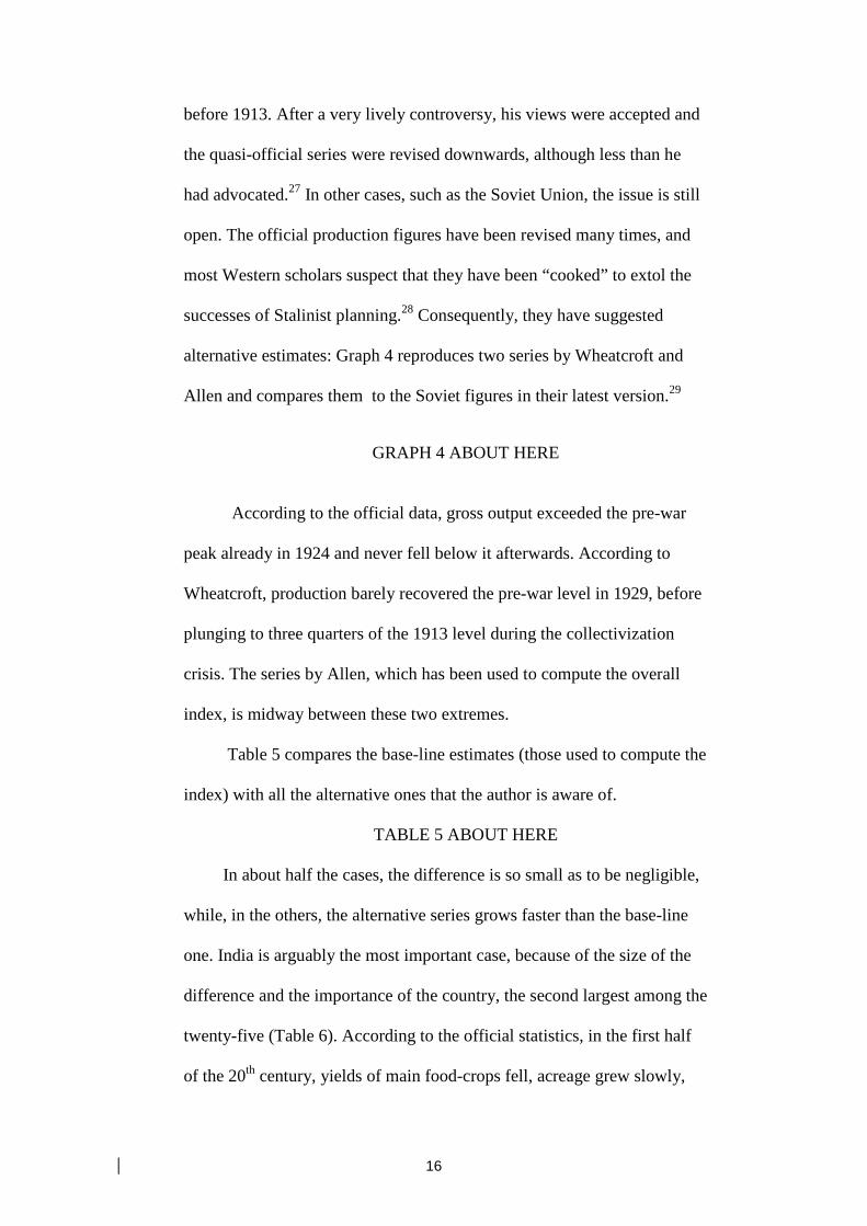
alternative estimates: Graph 4 reproduces two series by Wheatcroft and
Allen and compares them to the Soviet figures in their latest version.29
GRAPH 4 ABOUT HERE
According to the official data, gross output exceeded the pre-war
peak already in 1924 and never fell below it afterwards. According to
Wheatcroft, production barely recovered the pre-war level in 1929, before
plunging to three quarters of the 1913 level during the collectivization
crisis. The series by Allen, which has been used to compute the overall
index, is midway between these two extremes.
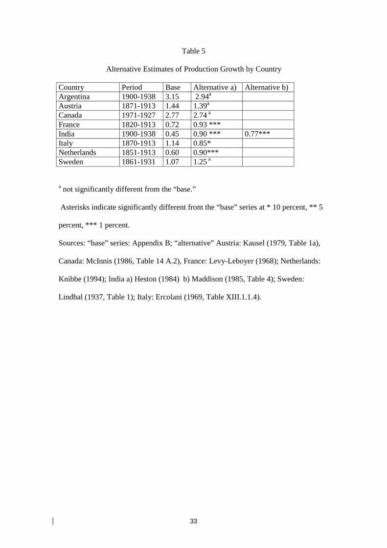
Table 5 compares the base-line estimates (those used to compute the
index) with all the alternative ones that the author is aware of.
TABLE 5 ABOUT HERE
In about half the cases, the difference is so small as to be negligible,
while, in the others, the alternative series grows faster than the base-line
one. India is arguably the most important case, because of the size of the
difference and the importance of the country, the second largest among the
twenty-five (Table 6). According to the official statistics, in the first half
of the 20th century, yields of main food-crops fell, acreage grew slowly,
17
and per capita consumption declined. This fall is controversial.
Sivasubramonian (2000), in his base-line estimate, endorses the official
production statistics, while other scholars deem a decline in consumption
implausible. Heston, in his own estimate of Indian GDP (alternative a),
revises the production data under the assumption that yields had remained
constant from the beginning of the century to the early 1950s.30
The two series thus imply quite different assessments of the
performance of Indian agriculture, with far-reaching implications for the
economic history of the country during the last period of British
domination. But the choice of one of them would not substantially affect
the analysis of “world” and area trends. Substituting the Sivasubramonian
series for Heston’s in 1900-38 would increase the Asian growth rate from
0.74 to 0.94 percent per year (causing production in 1938 to be 8 percent
higher) and the “world” rate by 0.02 points. Errors in country series must
be huge to affect the “world” index. For instance, a 100 percent mistake in
the American series leads to only 0.2 mistake in the “world” series in
1870-1913, and to a proportionally greater error in the series for smaller
countries. The “world” indices could be seriously biased only if several
country series were in error, and all in the same direction. This
coincidence cannot be ruled out, but it seems quite implausible.
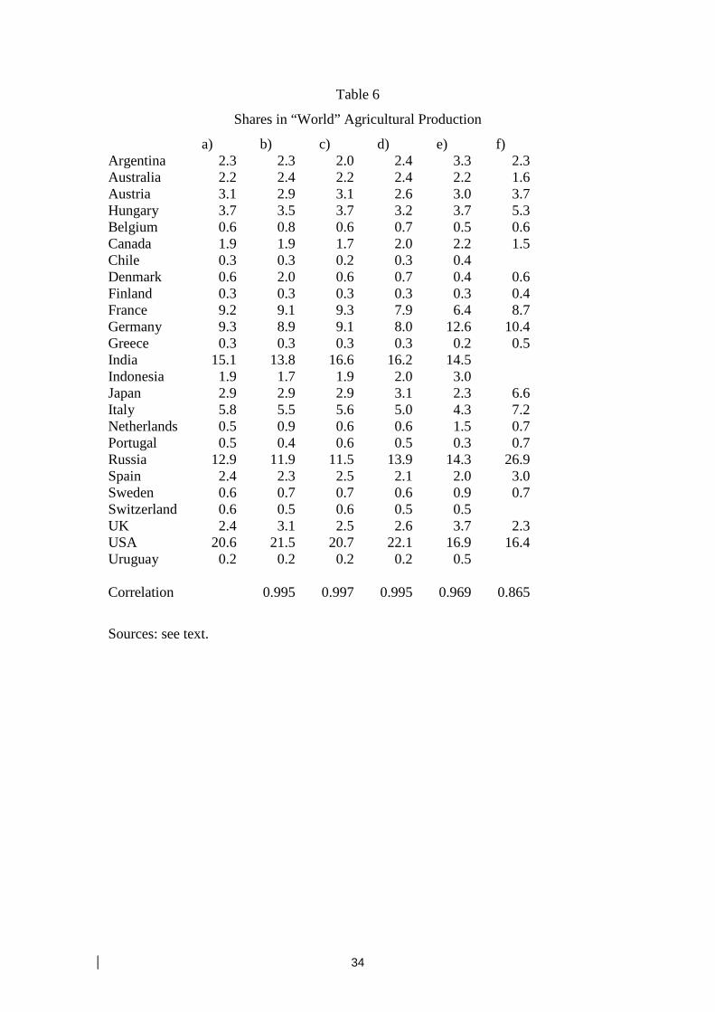
Mistakes in the weighting procedure are potentially more serious
than those in the country series. A wrong set of country shares might bias
the index upwards (downward) if fast-growing countries are given a too
high (low) weight. This can happen either because 1913 production in
those countries was unusually high (low) or because 1913 market
18
exchange rates overvalued (undervalued) the real purchasing power of the
country’s currency. Although agricultural products are highly tradable,
duties, quotas,and other trade barriers hampered trade. O’Brien and Prados
estimate that, in 1911, the market exchange rate overvalued the
“agricultural” Italian lira by 16 percent and the German mark by 10
percent.31 The effect of these potential biases can be explored by
computing the “world” indices with different weights (Table 6)
TABLE 6 ABOUT HERE
The two first columns on the left reproduce the “basic” country
shares (column a on “world” value added and column b on gross output).
Column c takes the short-term fluctuations into account by replacing gross
output in 1913 with an estimate for 1909-13.32 The three other columns
use different methods for converting the 1913 output into a common
monetary unit. The shares in column d are computed by simply reducing
the value of the output of the “protectionist” countries (Austria-Hungary,
Italy, France, Germany, Spain, Portugal and Sweden) by a fifth. Column e
uses the author’s estimate of the agricultural gross output for some 50
countries in 1913, which uses a standard set of international prices.33
Column f is calculated with the exchange rate implicit in Prados’s recent
estimates of national income in purchasing power parity in 1913.34
As shown in the bottom row, in three cases out of four, the
coefficients of correlation between the basic set of weights (column a) and
the alternative ones are extremely high and thus the long-run growth rates
are almost identical.35 The last set of weights (column f) differs from the
basic ones: as expected, the value of output is higher in “underdeveloped”
19
countries, such as Russia. However, the long-term growth rate of “world”
output comes out to be very close to the basic one (1.28 percent, instead of
1.33 percent for the same countries) and also the short term differences are
relatively small (cf. Graph 5).
GRAPH 5 ABOUT HERE
In short, this section shows that one can trust the overall reliability
of the “world” (and area) indices in spite of errors in some country series
and possibly in the weighting procedure.
VI EXTENSIONS: THE “OTHER” COUNTRIES
What happened in the rest of the world? Did agricultural production
increase as much as in the twenty five “core” countries? Table 7 provides
a partial answer. It reports the evidence on the growth of agricultural
production in a dozen other countries, which have been omitted from the
base series, because they do not cover the whole period 1870-1938 and/or
refer only to benchmark years.
TABLE 7 ABOUT HERE
By and large, these additional data confirm the previous results:
production increased in the long-run in almost all countries, and it grew
faster before rather than after World War One. Unfortunately, none of
these countries was really important from a worldwide perspective. Their
cumulated gross output in 1913 was about 6-7 percent of the “world”
total.36 It would be much more important to know something about China,
which in 1913 accounted for a quarter of world population and produced
20
about 20 percent more than the United States. Indeed, there are several
estimates, but, unfortunately, there is no consensus.37 Perkins, in his
classic book on Chinese agriculture, surmises that agricultural output
increased more or less as much as the population from 1850 to 1957 (i.e.,
at about 0.5 percent per year). Feuerwerker, in his authoritative survey of
Chinese economic history, endorses Perkins’ view, which is deemed too
optimistic by Chao, who implicitly suggests a growth of around 0.4
percent from 1882 to 1950.
Rawski disagrees. He argues that labor productivity must have
grown as much as real wages. If this were the case, agricultural output
must have grown much faster than Perkins assumed - by 1.4 to 1.7 percent
per year. from 1914/18 to the early 1930s. Rawski’s argument has not
convinced prominent Western scholars, such as Wiens and A. Maddison,
who, in his latest book, reinstates Perkins’ view. Output grew slightly
slower than population from 1890 to 1913, and slightly faster from 1913
to 1933. On the other hand, some years before, the Chinese scholar Wang
Yu-ru, apparently oblivious to the Western debate, had put forward a
figure (a growth rate of 1.2 percent from 1887 to 1928) which is only
marginally lower than Rawski’s “preferred” estimate. The end of the
debate is not in sight, but there is no doubt that total production grew
substantially, as the population increased from about 360 million in 1870
to about 500 in 1933 – i.e. by 40 percent (Maddison, 1998, Table D1).
As far as the author knows, there are no data, even tentative ones, on
agricultural production in all the other countries, including large areas of
Asia and almost the whole of Africa.38 Trends in agricultural production
21
can be inferred from the available, very tentative, estimates of change in
GDP per capita. Reynolds (1985) argued that, by 1870, “intensive growth”
(i.e., the increase in GDP per capita) had already started or was about to
start all over the world. His statement is buttressed by some recent
guesstimates by Maddison. He surmises that, from 1870 to 1950, the
average GDP per capita in the “rest of the world” (including China) grew
by a half.39 Such an increase must have augmented the demand for food,
which had to be satisfied by local production, as imports from the twenty-
five “core” countries were very small or negligible. A (conservative) back-
of-the-envelope estimate suggests that per capita production of foodstuffs
may have risen by a quarter.40 On top of this, exports of agricultural
products from most Third World countries grew quite substantially. Thus,
if Maddison is right, per capita agricultural production in the “rest of the
world” must have grown by at least by 25 percent from 1870 to 1938.
VII. EXTENSIONS: AN ESTIMATE OF TOTAL WORLD
OUTPUT
The rate of change in total world output can be estimated as an
average of the growth rates for the “core” twenty-five countries and for the
“rest of the world”, weighted with their respective share of output in 1913.
Unfortunately, the latter are not available. One can proxy them with the
proportion of output in 1970, or with the share of acreage (arable and tree-
crops) in the late 1940s, or with the percentage of the population in 1913.
The “rest of the world” accounted for about a third, two fifths and 45
percent of the total respectively.41 Clearly, none of these figures is an
22
exact proxy for their share of gross output, and it is difficult to assess a
priori whether they underestimate or overestimate the actual share. Thus,
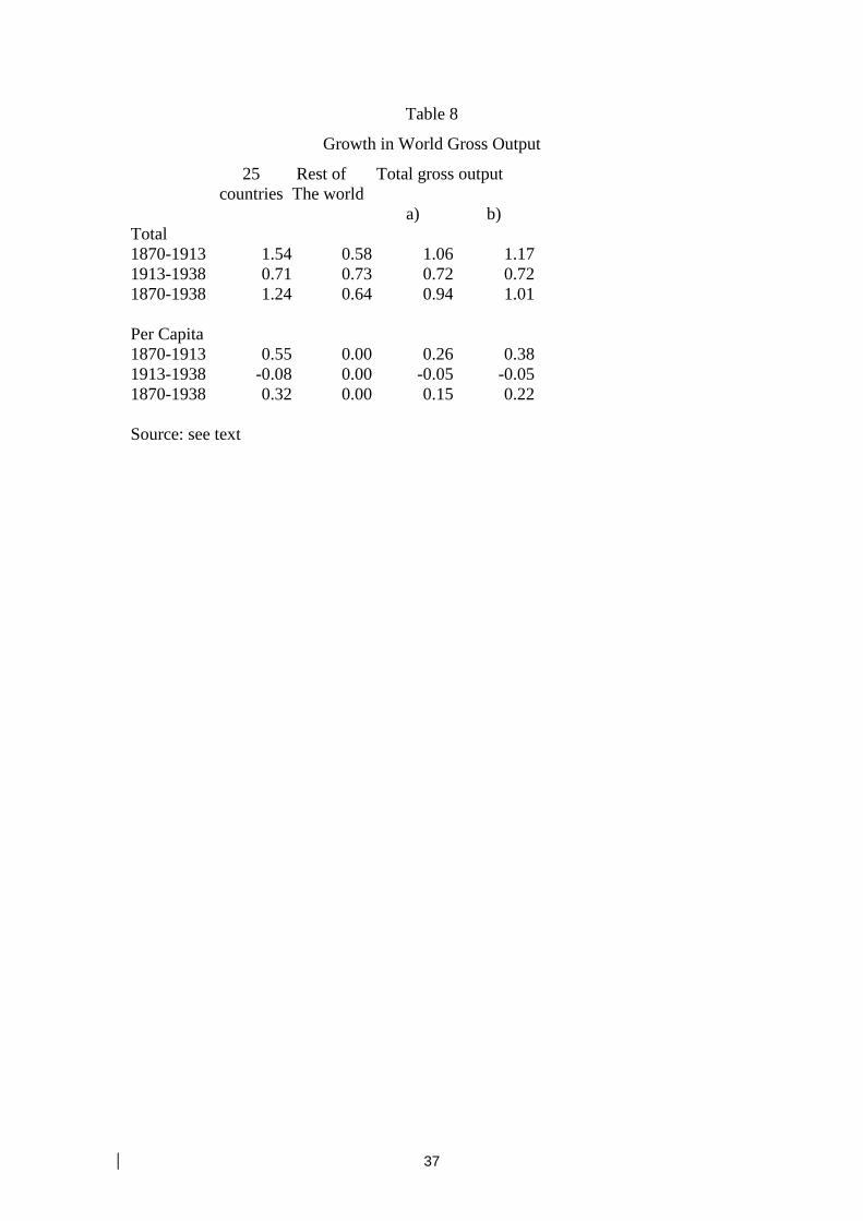
table 8 assumes that the “rest of the world” accounted for 45 percent
(column a) or 35 percent (column b) of world gross output. It also assumes
(conservatively) that its production per capita remained constant 42.
TABLE 8 ABOUT HERE
Needless to say, the estimate is highly tentative. However, it
confirms that the growth in total production was substantial, and that it
was decidedly faster before 1913 than after. The growth in production per
capita was not spectacular, nor was it negligible, either, especially in the
period before the war. Furthermore, if Reynolds and Maddison are right,
the estimate of Table 8 should be considered as a lower bound, with an
upper bound around 0.20 -0.30 percent per year. If this latter figure were
true, there would be very little difference between the performance before
and after World War Two. Even in the lower, more conservative, version,
the period would mark a clear discontinuity from the previous historical
experience. Maddison surmises that world GDP per capita (and thus also
agricultural output) grew at about 0.05 percent per year from 1000 to 1820
– i.e., by a half.43 This estimate seems too optimistic. In fact, according to
Allen (2000, Table 7) agricultural production per capita decreased in all
the major European countries from 1400 to 1800. It is unlikely that it had
increased in Europe before 1400, or in the rest of the world, sufficiently to
compensate for this loss and to achieve the long-run growth rate suggested
by Maddison. It seems more likely that agricultural production per capita
23
had remained roughly constant in pre-industrial times, albeit with wide
fluctuations.
VII. EXTENSION: THE CHANGES IN COMPOSITION
It is likely that the demand for agricultural products changed in the
long run for at least two reasons. First, industrialization must have
increased the demand for raw materials, and thus their share of total
agricultural production, because artificial substitutes were not available
before the 1920s (and their production boomed only after World War
Two). Second, the rise in income per capita must have increased the
demand, and thus the share, of high income-elastic goods. However, the
definition of the latter varied a lot by area: meat and dairy products were
“luxury” goods in Asia and Southern Europe, while they were almost the
staple diet in North-Western Europe, where the real luxuries were fruit
and vegetables. Unfortunately, testing these hypotheses is very difficult.
Only a few sources provide data by product, even if they estimate total
production.
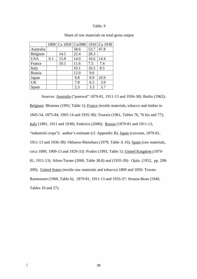
Table 9 shows the available data on the share of raw materials.
TABLE 9 ABOUT HERE
These data are not accurate. The Australian data refer to “pastoral”
production, inclusive of mutton, and thus overvalue the share of raw
materials. Other country data omit some products (notably wood from tree
crops), and thus undervalue the share, even if the bias is not likely to
exceed a few percentage points. In spite of these biases, the story is clear:
the share of raw materials was low in all countries except Australia and,
24
contrary to expectations, it did not increase over time – either decreasing
(as in France or the United Kingdom) or fluctuating without a clear trend
(as in the United States). In most countries, one or two goods (wool in
Australia and the United Kingdom, cotton in the United States, cocoons in
Japan and Italy) accounted for most of the aggregate “raw materials”.
The output of these “core” products was deeply affected by the state
of the world market, especially by competition from other countries,
which was almost never fettered by protection. For instance, the
production of British wool remained constant (and thus fell as a share of
total output) because of Australian competition. Unfortunately, the data
are too scarce to draw any meaningful inference on world trends.
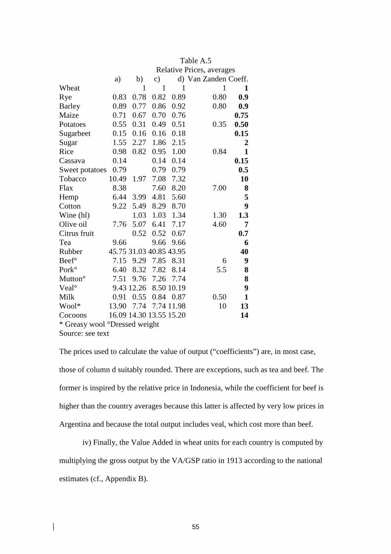
It is possible to be somewhat more precise about the distribution of
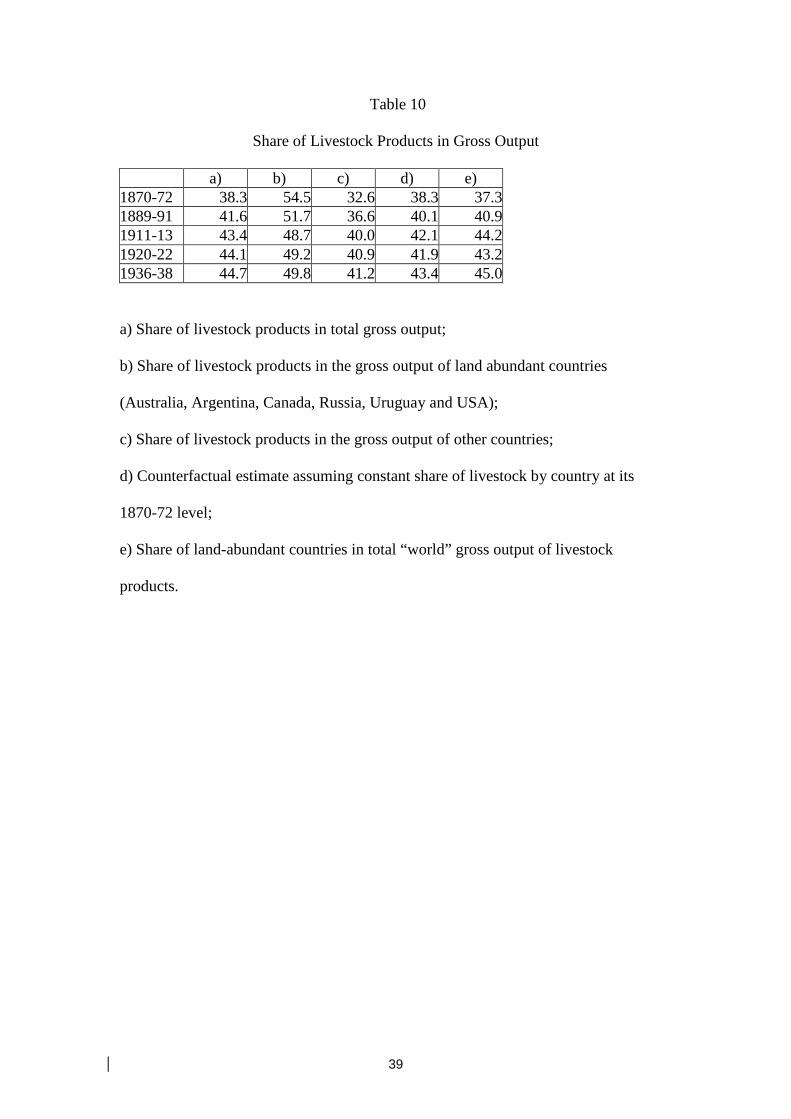
gross output between crops and livestock products (Table 10).44
TABLE 10 ABOUT HERE
As column a shows, the share of livestock products in gross output
of the twenty-five “core” countries grew substantially, especially before
World War One. The share of these countries in world totals has been
rising (Table 8), and livestock products accounted for a lower share in the
“rest of the world” than in the “core” countries. In 1913, they accounted
for about a quarter of gross output in a group of twenty-five other
countries, including China, Mexico and Turkey (Appendix A). Extending
(somewhat arbitrarily) this figure to the whole “rest of the world” for all
years, it is possible to estimate that the share of livestock products in
world gross output grew from about 30 percent in 1870 to about 35
percent in 1913, and remained almost stable thereafter. Relative prices of
25
livestock products increased substantially before 1913 and remained
roughly constant in interwar years, albeit with substantial fluctuations.45 A
contemporary increase in prices and production strongly suggests a
growing demand, not matched by an increase in (relative) productivity.
How was the growing demand for livestock products satisfied?
Traditional livestock-raising was quite a land-intensive activity, and thus
one would expect that it accounted for a greater share in land-abundant
countries (column b) than in the others (column c). Indeed, this was the
case at the beginning of the period: in 1870-1872, livestock products
accounted for 96 percent of Argentinian gross output and for a mere 17
percent of Indian output. Since then, their share declined in all land-
abundant countries except the United States, and rose in 15 out of the 19
land-scarce countries (the main exception being Indonesia).
This convergence is by no means surprising, given the underlying
change in factor endowment. However, this change in the country
composition of output only accounts for a fifth of the increase in the
“world” share of livestock products, as shown by a comparison of columns
d and a. The rest is accounted for by the growth in the share of land
abundant countries on the “world” output of livestock products (column
e). The population and incomes in these countries was growing faster than
in the rest of the “world” and these countries also supplied increasing
quantities of livestock products to (land-scarce) Europe.
VIII. CONCLUSIONS
The results of this paper can be summed up in five statements:
26
- agricultural output increased from the beginning of the nineteenth
century, and the growth accelerated over the century, peaking on the eve
of World War One. It was a veritable “golden age” for world agriculture,
as relative prices were rising or constant.
- the War and the Great Crisis hit agriculture quite hard, and growth
in the interwar years never reached the pre-war pace. However, prices did
not rise, even if they did not fall as catastrophically as has sometimes been
argued.
- The growth affected all areas, even if rates of increase were
decidedly greater in the countries of Western Settlement and in Eastern
Europe than in Asia and Western Europe.
- in the long run, the increase in output exceeded that of population
by a substantial margin especially in the Atlantic economy - but probably
throughout the world.
- the production of livestock products increased more than the total,
probably as a result of changes from the demand side.
These results answer, at least to some extent, the questions raised at
the beginning of this paper. But there is much work to be done. The main
priority is to add further countries to the sample, and to extend the existing
series back in time. Even imprecise estimates are better than total
ignorance. It would also be useful to revise several country estimates, even
if, as argued in section V, none of them would affect the world total that
much. In fact, accurate country series are essential in assessing country
performance. Last but surely not least, all this statistical ground-work is
only preliminary for tackling the real big issues: how was this growth
27
achieved? What was the contribution of productivity growth and technical
progress? How much did agricultural performance foster or hamper
modern economic growth?
28
Table 1 Rate of Growth of Agricultural Production and Population before 1870
Production Population Country Period Rate Period Rate Australia 1828-1870 8.42 1828-70 7.97 Austria 1830-1870 0.57 1840-70 0.63 Belgium 1812-1870 0.64 1816-66 0.30 Denmark 1818-1870 1.31 1801-70 0.95 France a) 1803-12/1870 0.90 1806-66 0.41 France b) 1821-1870 1.12 1821-66 0.50 England a) 1800-1870 1.10 1801-71 1.34 England b) 1800-1830 1.18 1801-31 1.18 England c) 1800-1850 1.00 1801-51 1.40 England d) 1800-09/1870-79 0.76 1801-71 1.34 Egypt 1821/1872-78 5.19 1821/1872-78 1.54 Germany a) 1800-10/1866-70 1.50 1817-70 0.91 Germany b) 1816-1849 2.61 1817-50 1.02 Germany c) 1800-10/1846-50 1.60 1817-50 1.02 Germany d) 1850-1870 1.49 1850-70 0.72 Indonesia 1815-7/1869-71 1.43 1820-70 0.96 Netherlands a) 1808-1870 1.10 1808-70 0.83 Netherlands b) 1851-1870 1.40 1851-70 0.75 Greece 1848-1870 2.72 1850-70 2.00 Poland 1809-1870 2.65 Na Portugal 1848-1870 -0.79 1841-78 0.53 Spain a) 1800-1870 0.57 1800-70 0.62 Spain b) 1850-1870 0.70 1857-77 0.36 Sweden 1800-1870 1.44 1800-70 0.82 United States 1800-1870 2.91 1800-70 2.88
Note: All data computed as geometric interpolations between three-years moving
averages (if not otherwise indicated)
Sources: Population data: Mitchell (1998a, b, and c, Tables A1 and A5).
Production data: Australia: Butlin-Sinclair (1986); Austria: Kausel (1979, Table 1a);
Sousa (1998); Spain: a) Gutierrez Brigas (2000, quadro VI.1), b) Prados (2000);
Sweden: Schon (1995, Table J1); United States: Weiss (1994, Table 1.6).
30
Table 2 Growth in Agricultural production, by Area and Period
Gross Output Value Added 1870-
1938 1870- 1913
1913- 1938
1870- 1938
1870- 1913
1913- 1938
Europe 1.19 1.36 0.76 a 1.05 1.30 -0.12a North Western Europe 0.97 1.02 1.50 0.74 0.90 1.41 Southern Europe 0.88 0.97 0.96 0.84 0.96 0.73 Eastern Europe 1.67 2.13 0.36 a 1.61 2.09 0.16 a Asia 0.97 1.11 0.58 0.96 1.18 0.56 South America 3.80 4.43 3.05 3.89 4.86 3.07 Western Settlement 1.37 2.20 0.74 1.22 1.92 0.62 World 1.31 1.56 0.67 1.18 1.48 0.38 a a not significantly different from zero Source: Statistical Appendix Table A1.
31
Table 3
Gross output 1915-18 (1913=100) Indices Other sources a) b) c) e) Asia 106.6 United Kingdom 114.5 96.8 99.2 Southern America 96.4 France 68.1 66.8 80.5 Western Settlement 102.8 Germany 67.3 67.5 62.2 European Neutral countriesa 99.6 Russia 79.0 74.9 81,1b Italy 87.6 Hungary 79.8 Austria 65.4b
a Denmark, Greece, the Netherlands, Portugal, Spain, Sweden, Switzerland
b 1915-17 only
Sources: Indices: Statistical Appendix Table I; a) League of Nations (1943) (cereals
and potatoes); b) Dessirer (1928) (cereals); c) United Kingdom: estimate of the author
Alternative Estimates of Production Growth by Country
Country Period Base Alternative a) Alternative b) Argentina 1900-1938 3.15 2.94a Austria 1871-1913 1.44 1.39a Canada 1971-1927 2.77 2.74 a France 1820-1913 0.72 0.93 *** India 1900-1938 0.45 0.90 *** 0.77*** Italy 1870-1913 1.14 0.85* Netherlands 1851-1913 0.60 0.90*** Sweden 1861-1931 1.07 1.25 a
a not significantly different from the “base.”
Asterisks indicate significantly different from the “base” series at * 10 percent, ** 5
Table 7 Rate of Growth in Agricultural Production, “Other” Countries
1870-1913 1913-1938 Bulgaria 1.14 Montenegro 2.12 Serbia 1.18 Egypt a) 2.19 0.94 Egypt b) 2.23 1.15 Palestine 7.39 Taiwan -0.91 2.85 Korea 2,76 Philippines 7.7 1.11 Thailand 1.32 2.20 Burma 0.14 -0.16 Mexico a) 2.92 -0.27 Mexico b) 3.35 2.02 Brazil 2.31 3.15 South Africa 2.55 New Zealand 3.94 1.61 Sources: Bulgaria (1865-73 to 1911-14), Montenegro (1873 to 1911-12) and Serbia
(1873-75 to 1911-12): Palairet (1997, Tables 7.1, 8.2 and 10.2) (total output); Egypt:
a) (1872-78 to 1910-14 and 1910-14 to 1935-39) O’Brien (1968, Table 10) (gross
output for eight major crops), b) (1887 to 1911-1913 and 1911-13 to 1936-38):
Hansen-Whattleworth (1978) (production); Palestine (1921-23 to 1936-39): Metzler
(1998, Table A.11) (gross output); Taiwan: (1887 to 1911-1913 and 1911-13 to
1936-38) and Korea (1911-13 to 1936-39): Mizoguchi-Umemura (1988, Tables 5 and
7) (NDP at factor costs), Philippines: (1902-18 and 1918-1938): Crisostomo-Barker
(1979, Table 5.1); Thailand (1870-1913 and 1913-1938): Manarungsan (1989, Table
c.3) (GDP at market prices); Burma (1901-2 to 1911-12 and 1911-12 to 1938-39):
Saito-Kong (1999, Table IX-2) (NDP at factor costs); Mexico a) (1900-02 to 1911-
13) Carr (1973, Table 1) (“total output”), b) (1900-1910 and 1910-1940): Reynolds
(1970, Table 3.2) (“production”); Brazil (1901-1911 and 1911-1941): Merrick-
Graham (1979, Table II.3); South Africa (1911-13 to 1936-38): Union of South Africa
36
(1960, Table I-27) (“physical output”); New Zealand (1900-1910; 1910 to 1936-38):
Bloomfield (1984) (gross output Table v.3 deflated with wholesale prices IX.13 and
IX.14)
37
Table 8
Growth in World Gross Output
25
countries Rest of The world
Total gross output
a) b) Total 1870-1913 1.54 0.58 1.06 1.171913-1938 0.71 0.73 0.72 0.721870-1938 1.24 0.64 0.94 1.01 Per Capita 1870-1913 0.55 0.00 0.26 0.381913-1938 -0.08 0.00 -0.05 -0.051870-1938 0.32 0.00 0.15 0.22 Source: see text
38
Table. 9
Share of raw materials on total gross output
1800 Ca 1850 Ca1880 1910 Ca 1938 Australia 58.6 53.7 47.8 Belgium 14.5 22.4 28.3 USA 6.1 15.8 14.0 16.6 14.4 France 10.1 11.6 7.5 7.4 Italy 10.1 10.5 8.5 Russia 12.0 9.6 Japan 9.8 8.9 10.9 UK 7.8 6.5 3.9 Spain 2.3 3.3 3.7
Sources: Australia (“pastoral” 1879-81, 1911-13 and 1936-38): Butlin (1962);
Belgium: Blomme (1993, Table 1); France (textile materials, tobacco and timber in
1845-54, 1875-84, 1905-14 and 1935-38): Toutain (1961, Tables 76, 76 bis and 77);
Italy (1891, 1911 and 1938): Federico (2000); Russia (1879-81 and 1911-13,
“industrial crops”): author’s estimate (cf. Appendix B); Japan (cocoons, 1879-81,
1911-13 and 1936-38): Okhawa-Shinohara (1979, Table A 16); Spain (raw materials,
circa 1890, 1909-13 and 1929-33): Prados (1993, Table 1); United Kingdom (1879-
81, 1911-13): Afton-Turner (2000, Table 38.8) and (1935-39): Ojala (1952, pp. 208-
209); United States (textile raw materials and tobacco) 1800 and 1850: Towne-
Rasmussen (1960, Table 6), 1879-81, 1911-13 and 1935-37: Strauss-Bean (1940,
Tables 10 and 27).
39
Table 10
Share of Livestock Products in Gross Output a) b) c) d) e) 1870-72 38.3 54.5 32.6 38.3 37.31889-91 41.6 51.7 36.6 40.1 40.91911-13 43.4 48.7 40.0 42.1 44.21920-22 44.1 49.2 40.9 41.9 43.21936-38 44.7 49.8 41.2 43.4 45.0
a) Share of livestock products in total gross output;
b) Share of livestock products in the gross output of land abundant countries
(Australia, Argentina, Canada, Russia, Uruguay and USA);
c) Share of livestock products in the gross output of other countries;
d) Counterfactual estimate assuming constant share of livestock by country at its
1870-72 level;
e) Share of land-abundant countries in total “world” gross output of livestock
products.
40
50
60
70
80
90
100
110
120
130
1870 1880 1890 1900 1910 1920 1930
GDP GSP
Graph 1Agricultural production
41
0
40
80
120
160
200
1870 1880 1890 1900 1910 1920 1930
EuropeAsia
South AmericaWestern Settlement
Graph.2Agricultural output, by continent
42
1870 1880 1890 1900 1910 1920 1930
Eastern Southern North-Western
Graph.3Agricultural output, Europe
43
40
60
80
100
120
140
20 22 24 26 28 30 32 34 36 38
URSSOFFICIAL URSSWHEATCROFT RUSSIAOUTPUT
Graph. 4Alternative estimates of Soviet gross output
(1913=100)
44
40
50
60
70
80
90
100
110
120
1870 1880 1890 1900 1910 1920 1930
GDP GDPPRADOS
Graph. 5Indexes of output, with alternative weighting schemes
45
APPENDIX A
The estimate of “PPP-adjusted” agricultural production in 1913
The PPP-adjusted production in 1913 is computed for forty-nine
countries, the twenty-three of the sample and twenty-six others, including
China (cf. the full list in Table A.6). The computation follows the three-
step usual procedure: 1) estimate total production; 2) deduct seed and
feed; 3) multiply by “world” prices to obtain gross output and 4) deduct
expenditures on purchased materials to get Value Added.
1) Production is computed taking twenty-three products into
Cocoon 11.00 * Greasy wool °Dressed weight Sources: UK a) Paish (1913-14, pp. 556-570) except rubber from Stillson (1971, Table 1); USA a) U. S. Bureau of the Census (1975, series K
A.3) and some additional country sources.66 When necessary, figures have been
obtained by linear interpolation.
There are several estimates of the world population at different dates, which are
reported for the reader’s ease in Table C.1
74
Table C.1
Estimates of World Population (millions) 1850 1870 1875 1900 Biraben Mc Evedy MaddisonMc Evedy Biraben Clark Mc Evedy Maddison Europe 288 279 324 422 411 415 North America 25 34 57 90 81 95 South Central America 34 25 40 34 75 63 50 81 Africa 102 81 91 93 138 122 110 125 Asia 790 781 765 817 903 985 946 978 Oceania 2 1 2 6 6 7 Europe and Western Offshoots 375 608 Total: World 1.241 1.201 1.270 1.326 1.634 1.668 1.622 1.791 1925 1930 1937 1940 1950 Mc Evedy UN Clark IIA UN Clark Biraben UN Europe 513 531 532 557 551 573 575 547 North America 140 135 135 159 146 146 166 172 South Central America 81 109 109 104 131 131 164 167 Africa 140 155 157 168 172 176 219 221 Asia 1.107 1.047 1.141 1.138 1.202 1.233 1.393 1.402 Oceania 10 10 10 11 11 11 13 13 Europe and Western Offshoots
Total: World 1.990 1.987 2.084 2.137 2.214 2.270 2.530 2.522
Sources: Biraben (1979), McEvedy-Jones (1978), Clark (1977), United Nations
1920-1940 (1952, Table 1A) (average of maximum and minimum estimates), 1950
UN demographic yearbook 1999; Maddison (2001, Table A-c)
75
As one can see, they broadly agree, even if many figures are pure guesstimates. The
population data (Table C 2) are thus taken from Maddison for 1870 and 1913, the
United Nations for 1920 and the Institute Internationale d’Agriculture for 1938 (the
1937 figure increased by 1.5 percent to take account of the natural increase of
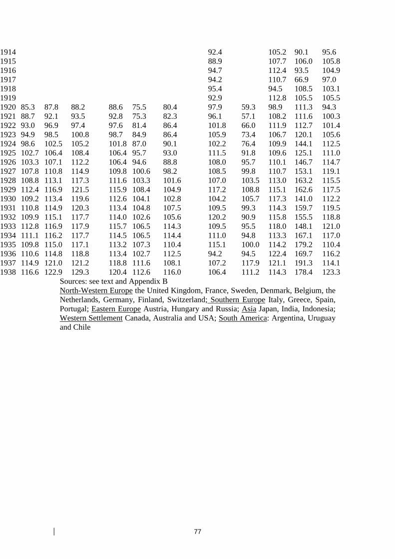
Sources: see text and Appendix B North-Western Europe the United Kingdom, France, Sweden, Denmark, Belgium, the Netherlands, Germany, Finland, Switzerland; Southern Europe Italy, Greece, Spain, Portugal; Eastern Europe Austria, Hungary and Russia; Asia Japan, India, Indonesia; Western Settlement Canada, Australia and USA; South America: Argentina, Uruguay and Chile
78
Statistical Appendix Table II
Rates of change in GDP, by country 1870-
1938 1870-1913
1913 -1938
Column Difference
Argentina 4.41 6.07 2.89 *** Australia 2.83 3.36 2.31 *** Austria 1.09 1.44 1.52° * Hungary 1.46 2.26 0.07° *** Belgium 0.62 0.76 0.02° *** Canada 2.00 2.86 -1.06 *** Chile 1.86 1.56 1.88 a
Denmark 1.87 1.62 3.24 * Finland 1.26 1.56 1.89 a France 0.58 0.62 0.90 a Germany 0.91 1.56 0.02° *** Greece 1.53 2.12 3.56° *** India 0.73 0.96 0.31 *** Indonesia 1.97 1.79 1.92 a Italy 0.86 1.14 0.58 *** Japan 1.60 1.73 0.75 ** Netherlands 1.31 0.65 2.47 *** Portugal 0.87 0.54 3.17 *** Russia 1.79 2.24 0.02° *** Spain 0.69 0.46 -0.06° *** Sweden 1.03 0.96 1.49 a Switzerland 0.72 0.70 0.83 a UK 0.58 0.00° 1.52 ** USA 1.12 1.70 0.56 ** Uruguay 3.16 2.91 5.25 *** Column Difference: test of the difference between the growth rates in 1870-1913 and 1913-1938: a not significant; Significantly different from zero at * 10 percent, ** 5 percent and *** 1 percent.
79
BIBLIOGRAPHY
Adamets, S. (1997). ‘A’ l’origine de la Diversité des Measures de la Famine
Sovietique: La Statistique des Prix, des Récoltes et de la
Consommation’ Cahiers du Monde Russe 38: 559-586.
Afton B. and M.Turner. (2000). “The Statistical Base of Agricultural
Performance in England and Wales, 1850-1914”. In The Agrarian
History of England and Wales, Vol VII 1850-1914, E. J.T. Collins ed..
Cambridge: Cambridge University Press.
Akarli, A. (2000). “ Growth and retardation in Ottoman Macedonia, 1880-
1910.” In The Mediterranean Response to Globalisation before 1950 ,
S. Pamuk, and J. Williamson eds.. London: Routledge.
Allen, R. (1994). “Agriculture during the Industrial Revolution’ In The
Economic History of Britain since 1700, vol 1. 2nd edition, D.
McCloskey and R. Floud eds.. Cambridge: Cambridge University
Press.
Allen, R. (1999). “Tracking the Agricultural Revolution in England.”
Economic History Review 52: 209-235.
Allen R. (2002). Farm to Factory: a Reinterpretation of the Soviet
Industrial Revolution (unpublished manuscript).
80
Arndt, H.W. (1963). The Economic Lessons of the Nineteen-Thirties 2nd ed.
London: Frank Cass.
Bairoch, P. (1999). L’agriculture des Pays Développés. 1800 à nos Jours.
Paris: Economica.
Baten, J. (2000). “Heights and Real Wages in the 18th and 19th Centuries: an
International Overview” Historische Anthropometrie, special issue of
the Jahrbuch fur Wirtschaftsgeschichte: 62-76.
Bértola L. (1998). El PBI Uruguayo 1870-1936 y Otras Estimaciones.
Montevideo : Facultad de Ciencias Sociales.
Biraben, J. N. (1979). "Essai sur le Nombre des Hommes" Population 34:
13-24.
Blomme, J. (1992). The Economic Development of Belgian Agriculture
1880-1980. A Qualitative and Quantitative Analysis. Leuwen: Leuwen
University Press
Blomme, J. (1992). "Produktie, Produktiefactor en Produktivitiet: de
Belgische Landbouw in de 19de Eeuw" Belgisch Tijdschrift voor
Nieuwste Geschiedenis 25: 103-114
81
Bloomfield, B.T. (1984). New Zealand : A Handbook of Historical
Statistics. Boston: Hall & Co.
Blyn, G. (1966). Agricultural Trends in India, 1891-1947: Output,
Availability, and Productivity. Philadelphia: University of
Pennsylvania Press.
Brandt, L. (1989). Commercialization and Agricultural Development.
Central and Eastern China, 1870-1937. New York: Cambridge
University Press.
Brandt, L. (1997). “Reflections on China’s late 19th and early 20th Century
Economy.” China Quartely 150: 282-307.
Braun, J. M., I. Braun, J. D. Briones, R. Luders, G. Wagner. (2000).
Economia Chilena 1810-1995: Estadisticas Historicas. Documentos
de trabajo n.187 Pontificia Universidad catolica de Chile Instituto de
Lewis, W. A. (1978). Growth and Fluctuations. London: Allen and Unwin.
Lindahl, E. et al. (1937). National Income of Sweden 1861-1930. London:
King.
MacPherson, W. J. (1987). The Economic Development of Japan c. 1868-
1941. London and Basingstoke: MacMillan.
94
Maddison, A. (1985). “Alternative Estimates of the Real Product of India,
1900-1946.” The Indian Economic and Social History Review 22: 201-
210.
Maddison, A. (1991). Dynamic Forces in Capitalist Development. Oxford:
Oxford University Press.
Maddison, A. (1995). Monitoring the World Economy. Paris: OECD.
Maddison, A. (1998). Chinese Economic Performance in the Long Run.
Paris: OECD.
Maddison, A. (2001). The World Economy. A Millennial Perspective Paris :
OECD.
Malle, S. (1985). The Economic Organization of War Communism, 1918-
1921. Cambridge: Cambridge University Press.
Manarungsan, S. (1989). Economic Development of Thailand, 1850-1950.
Response to the Challenge of the World Economy. Bangkok,
Chulalongkorn University. Institute of Asian Studies, Monograph n.
042.
95
Mancall, P. C. and T. Weiss. (1999). “Was Economic Growth Likely in
Colonial British North America?” Journal of Economic History 59:
17-40.
McAlpin, M. (1983). “Price Movements and Fluctuations in Economic
Activity.” In The Cambridge Economic History of India. II. c. 1757-c.
1970, D. Kumar and M. Desai eds.. Cambridge: Cambridge University
Press.
McCarthy, J. (1982). The Arab World, Turkey and the Balkans: a Handbook
of Historical Statistics. Boston: Hall & Co..
McInnis, M. (1986). “Output and Productivity in Canadian Agriculture,
1870-71 to 1926-27.” In Long Term Factors in American Economic
Growth, S. Engerman, and R. E. Gallman eds.. Chicago: University of
Chicago Press.
Merrick T. W. and D.H. .Graham. (1979). Population and Economic
Development in Brazil, 1800 to the Present. Baltimore and London:
John Hopkins University Press.
Metzler, J. (1998). The Divided Economy of Mandatary Palestine.
Cambridge: Cambridge University Press.
96
Mishra, S. C. (1983). ‘On the Reliability of pre-Independence Agricultural
Statistics in Bombay and Punjab’ The Indian Economic and Social
History Review 20: 171-190.
Mitchell, B. R. (1988). British Historical Statistics. Cambridge: Cambridge
University Press.
Mitchell, B. R. (1998a). International Historical Statistics: Africa, Asia,
Oceania 1750-1993. 3rd ed. London: MacMillan.
Mitchell, B. R. (1998b). International Historical Statistics: the Americas
1750-1993. 4th ed. London: MacMillan.
Mitchell, B. R. (1998c). International Historical Statistics: Europe 1750-
1993. 4th ed. London: MacMillan.
Mizoguchi, T. and Umemura, M. (1988). Basic Economic Statistics of
former Japanese Colonies, 1895-1938. Tokyo: Keizai Shinposha.
Moore, W. E. (1945). Economic Demography of Eastern and Southern
Europe. Geneva: League of Nations.
97
Mosley, P. (1983) The Settler Economies. Studies in the Economic History
of Kenya and Southern Rhodesia 1900-1983. Cambridge: Cambridge
University Press.
Nakamura, J. L. (1966). Agricultural Production and the Economic
Development of Japan 1873-1922. Princeton: Princeton University
Press.
O’Brien, P. (1968). “The Long-Term Growth of Agricultural Production in
Egypt: 1821-1962.” In Political and Social Change in Modern Egypt,
P.M. Holt ed.. London
O’Brien, P. and L. Prados de la Escosura. (1992). “Agricultural Productivity
and European Industrialization” Economic History Review 51: 514-36.
Offer A. (1989). The First World War: An Agrarian Interpretation. Oxford:
Clarendon Press.
O’Grada, C. (1991). “Irish agriculture. North and South since 1900.” In
Land, Labour and Livestock: Historical Studies in European
Agricultural Productivity, B. M. Campbell and M. Overton eds..
Manchester: Manchester University Press.
O’Grada, C. (1993). Ireland before and after the Famine, 2nd ed..
Manchester: Manchester University Press.
98
Ojala, E.M. (1952). Agriculture and Economic Progress. Oxford: Oxford
University Press.
Okhawa, K. (1967). “Prices.” Long Term Economic Statistics of Japan Vol
8. K.Okhawa, M.Shinohara and M.Umemura, eds.. Tokyo: Keizai
Shinposha.
Okhawa, K. and Shinohara, M. (1979). Patterns of Japanese Economic
Development. New Haven and London: Yale University Press.
Overton, M. (1996). Agricultural Revolution in England. Cambridge:
Cambridge University Press.
Paish, G. (1913-14). “On Prices of Commodities in 1914.” Journal of the
Royal Statistical Society 77: 565-70.
Palairet, M. (1997). The Balkan Economies. Cambridge: Cambridge
University Press.
Perkins, D. (1968). Agricultural Development in China. Edinburgh:
Edinburgh University Press.
99
Petmezas, S. (1999). “Revising the Estimates for the Agricultural Output of
Greece (1833-1939).” In Third conference of the European Historical
Economics Society. Lisbon, October 29-30, 1999.
Prados de la Escosura, L. (1989). “La Estimacion Indirecta de la Produccion
Agraria en el siglo XIX: Replica a Simpson.” Revista de Historia
Economica 7: 703-717.
Prados de la Escosura, L. (1993). Spain’s Gross Domestic product, 1850-
1990: a New Series. Madrid: Ministerio de Economia Y Hacienda.
Documentos de Trabajo D-93002.
Prados de la Escosura, L. (2000). “International Comparisons of Real
Product, 1820-1990: an Alternative Data-set.” Explorations in
Economic History 37: 1-41.
Pray, C. E. (1984). “Accuracy of Official Agricultural Statistics and the
Sources of Growth in the Punjab 1907-47,” The Indian Economic and
Social History Review 21: 312-333.
Pryor, F. et al. (1971). ‘Czechoslovak Aggregate Production in the Interwar
Period.” Review of Income and Wealth 1: 35-60.
100
Rao, P. (1993) Intercountry Comparisons of Agricultural Output and
Productivity. Rome: FAO Economic and social development paper
112.
Rosenberg, N. and L. Birdzell. (1986). How the West Grew Rich. New
York: Basic Books.
Rawski, T. (1989). Economic Growth in pre-war China. Berkeley:
University of California Press.
Reynolds, C. W. (1970). The Mexican Economy. Twentieth-Century
Structure and Growth. New Haven and London: Yale University
Press.
Reynolds, L. G. (1985). Economic Growth in the Third world: an
Introduction. New Haven and London: Yale University Press.
Richardson, P. (1999). Economic Change in China, c. 1800-1950.
Cambridge: Cambridge University Press.
Ritzmann-Blickenstorfer T. and T. David (no date). Un Image Statistique du
Developpment Economique en Suisse. Personnes Actives Et Produit
Interieur Brut par Branches et Cantons, 1890-1965. Lausanne:
Université de Lausanne, Mimeo.
101
Roy, T. (2000). The Economic History of India, 1857-1947. Oxford: Oxford
University Press.
Saito, T. and K. L. Kin. (1999). Statistics on the Burmese Economy.
Singapore: The 19th and 20th Century Institute of Southeast Asian
Studies.
Sandgruber, R. (1978). Osterreisches Agrarstatistik 1750-1918. Munich:
????.
Schilcher L. (1991). “The Grain Economy of Late Ottoman Syria and the
Issue of Large Scale Commercialisation.” In Landholding and
Commercial Agriculture in the Middle East, C. Keyder and F. Tabak.
eds. New York: State University of New York Press
Schon, L. (1995). Jordbruk med Binäringar, 1800-1980, Lund: Skrifter
Utgivna av Ekonomisk-Historika Föreningen i Lund, vol XXIV.
Schultze, M. S. (2000) “Pattern of Growth and Stagnation in the Late
Nineteenth Habsburg Economy“ European Review of Economic
History 4: 311-340.
Schultze, M. S. (2002) “Austria-Hungary“Paper delivered to the Warwick
research seminar on The Economics of Word War One
102
Simpson, J. (1989a). “La Produccion Agraria y el Consumo Espanol en el
Siglo XIX.” Revista De Historia Economica 7: 355-388.
Simpson, J. (1989b). “Una Respuesta al Profesor Leandro Prados de la
Escosura.” Revista de Historia Economica 7: 719-23.
Sivasubramonian, S. (2000). The National Income of India in the Twentieth
Century. New Delhi: Oxford University Press.
Statistics Canada. 1983. Historical Statistics of Canada. 2nd ed., edited by
F.H. Leacy: Ottawa.
Steckel, R. H. (1995). “Stature and the Standard of Living.” Journal of
Economic Literature 33: 1903-1940.
Steckel, R. H. (1998). “Strategic Ideas in the Rise of Anthropometric
History and their Implications for Interdisciplinary Research’ Journal
of Economic History 58: 803-821.
Steckel, R. and R. Floud. (1997). ‘Conclusions’. In Health and Welfare
during Industrialization. R. Steckel and R. Floud eds.. Chicago:
University of Chicago Press for NBER.
103
Stillson, R. T. (1971). “The Financing of Malayan Rubber, 1905-1923.”
Economic History Review 24: 589-98.
Strauss, Frederick and L. H. Bean. (1940). “Gross Farm Income and Indices
of Farm Production and Prices in the United States 1869-1937.”
United States Department of Agriculture Technical Bulletin n. 703.
Washington: Government Printing Office.
Tilly, R. H. (1978). “Capital Formation in Germany in the Nineteenth
Century.” In The Cambridge Economic History Of Europe vol. VII pt.
1. P.Mathias and M. M.Postan, eds.. Cambridge: Cambridge
University Press.
Toutain, J. C. (1961). “Le Produit de l’Agriculture Française de 1700 a
1958” [“Histoire quantitative de l’economie française” (1) and (2)].
Cahiers de l’Institut de Science Economique Appliquee. Serie AF 1
and 2. Paris: ISEA.
Toutain, J. C. 1997. “La Croissance Française 1789-1990. Nouvelles
Estimations.” Economies et sociétés. Cahiers de l’ISMEA. Serie
Histoire quantitative de l’economie francaise. Serie HEQ n.1. Paris:
????
Towne, M. W. and W. D. Rasmussen. (1960). “Farm Gross Product and
Gross Investment in the Nineteenth Century.” In Trends In The
104
American Economy In The Nineteenth Century. (Studies in income and
wealth. Vol. 24). Princeton: Princeton University Press.
Turner, M. (1996). After the Famine. Irish Agriculture 1850-1914.
Cambridge: Cambridge University Press.
Turner, M. (2000). “Agricultural Output, Income and Productivity” In The
Agrarian History of England and Wales vol VII 1850-1914, E. J.T.
Collins, ed.. Cambridge: Cambridge University Press
United Nations. (various years) United Nations Demographic Yearbook.
Geneva: United Nations
Union of South Africa. (1960). Union Statistics for Fifty Years. Jubilee
Issue, 1910-1960. Pretoria: Bureau of Census and Statistics.
Urquhart, M.C. (1993). Gross National Product, Canada 1870-1926: The
Derivation of the Estimates. Kingston & Montreal: McGill and Queens
University Presses.
Van der Eng, P. (1996). Agricultural Growth in Indonesia. London and
Basingstoke: Macmillan.
Van Zanden, J. L. (1988). “The First Green Revolution: The Growth of
Production and Productivity in European Agriculture 1870-1914.”
105
Research Memorandum 42 . Amsterdam: Vrije Universiteit Facultit
der Economische Wetenschappen en Econometrie.
Van Zanden, J. L. (2000). “Estimates of GNP.” Available at
http://nationalaccounts.niwi.knaw.nl.
Van Zanden J. L. (2003). “Rich and Poor before the Industrial Revolution:
A Comparison Between Java and the Netherlands at the Beginning of
the 19th Century.” Explorations in Economic History 40:1-23.
Vinsky, I. (1961). “National Product and Fixed Assets in the Territory of
Yugoslavia 1961.” In Studies in Social and Financial Accounting.
Income and wealth series, vol. 9. P. Deane, ed. London
Visaria, L. and Visaria, P. (1983). “Population (1757-1947).” In The
Cambridge Economic History of India. II. c. 1757-c. 1970, D. Kumar
and M. Desai, eds.. Cambridge: Cambridge University Press.
Von Jankovich, B. (1912). “Index-Number von 45 Waaren in der
Oesterreisch-Ungarischen Monarchie (1867-1909).” Bulletin de
l’InstitutIinternationale de la Statistique 19, 3 : 136-156.
Waizner, E. (1928). “Das Volkseinkommen Alt-Osterreichs und seine
Vertellung auf die Nachfolgestaaten.” Metron 7: 97-179.
106
Warren G. and F. A. Pearson. (1937). World Prices and the Building
Industry. New York: Wiley and Sons.
Wang, Y. (1992). “Economic Development in China between the Two
World Wars (1920-1936).” In The Chinese Economy in the early
Twentieth Century. Recent Chinese studies, edited by ???? Wright.
New York: St Martin’s Press.
Weiss, T. (1994). “Economic Growth before 1860: Revised Conjectures.” In
American Economic Development in Historical Perspective, T. Weiss
and D. Schaefer, eds.. Stanford: Stanford University Press.
Wheatcroft, S. G. (1990). “Agriculture.” In From Tsarism to the New
Economic Policy, R.W.Davies (ed.), London and Basingstoke:
Macmillan
Wheatcroft, S.G. and R.W. Davies (1994a). ‘The Crooked Mirror of Soviet
Economic Statistics’. In The Economic Transformation of the Soviet
Union, 1913-1945, R.W. Davies, M. Harrison and S. G. Wheatcroft
eds.. Cambridge: Cambridge University Press.
Wheatcroft, S. G. and R. W. Davies. (1994b). “Agriculture” In The
Economic Transformation of the Soviet Union, 1913-1945, R.W.
Davies, M. Harrison and S.G. Wheatcroft eds.. Cambridge: Cambridge
University Press.
107
Wiens, T. B. (1992). “Trends in the late Qing and Republican Rural
Economy: Reality or Illusion?” In “New Perspectives on the Chinese
Rural Economy: a Symposium,” D. Little, ed. Republican China 18:
63-76.
Williamson, J. (1999). “Labor and Globalization in the Pre-Industrial Third
World.” Paper presented to the ESF Conference on Historical Market
Integration: Performance and Efficiency of Markets in the Past.
Venice, December 17-20, 1999.
Williamson, J. and K. O’Rourke. (1999). Globalization and History.
Cambridge (Mass): MIT Press.
108
NOTES * The author thanks B. Allen, T. David, S. Fenoaltea, P. Lains, D. Ma, S. Pamuk, S. Petmezas, L. Prados, M.S. Schultze, A. Taylor, P. Van der Eng, J. L. Van Zanden and J. Williamson for having provided highly useful information and shared with me the results of their research before publication, and the participants to seminars at UC-Los Angeles and UC-Davis, and to the Fourth World Cliometric Conference (Montreal 5-9 July 2000) for their comments on earlier versions of the paper (published as Working paper n.103 of the Agricultural History Center. University of California at Davis). The remaining errors are mine. The data are available at http://www.iue.it/HEC/People/Faculty/Profiles/Federico.shtml
1 Population from Maddison (2001), calories from FAO (www.fao.org).
2 Fogel (1997, p. 450). The long-run growth in caloric availability is
shown also by the rise in heights.
3 The first figure is estimated from FAO, Yearbook, various years. It
excludes the Communist countries, and thus may overvalue actual
growth. The data for 1961-2000 are taken from the FAO website
(www.fao.org).
4 The role of agricultural crisis was first highlighted by Arndt (1963, p.
10). Cf. for instance Feinsten et al (1997, pp. 78-80) or James (2001, pp.
112-113).
5 Price trends will be dealt with succinctly, on the basis of the discussion
in Federico forthcoming, ch. 3.3
6 In the following, the word “world” is written between brackets when it
refers to the 25 countries covered in the index and without brackets
when it refers to all countries.
7 Cf., Rao (1993 pp. 12-14). In the following, the words “output” and
“gross output” will be used for GDP and GSP respectively, while
“production” refers to both.
109
8 For a detailed description of the data, sources, and methods, see
Appendix B. The missing (and interpolated) years are 1870-1873 for
Japan, 1870-74 for Argentina, 1870-1879 for Belgium and Indonesia,
1870-71 and 1873-81 and 1883 for India, 1920-24 for Germany and the
Soviet Union. When necessary, gross output (value added) is estimated
starting from value added (gross output) with information provided by
the source itself or with VA/GSP ratios for similar countries. Some
series adopt slightly different concepts (e.g., the net instead of gross
domestic products), and these differences are taken into account
whenever possible. Boundaries are adjusted to those existing in 1913
with data on output or, when the latter are not available, on agricultural
acreage. In this case, it is implicitly assumed that the production per acre
was similar throughout the whole country.
9 The omission of forestry, fishing, and hunting reduces the bias in the
series for countries of Western Settlement arising from the omission of
the output by native population. Their contribution to agriculture was
minimal, while they accounted for a sizeable, even if fast shrinking,
share of the total primary output in the USA (Mancall-Weiss, 1999) and
Australia (Butlin-Sinclair, 1986) in the 18th and early 19th century.
10 Exchange rates from League of Nations 1913-1925. The effect of
alternative methods of conversion (wheat units and PPP-adjusted
exchange rates, etc.,) is explored in section five.
11 The extent of the fall in Portuguese production depends a lot on the
starting point. Omitting 1848 (an exceptionally good year) the rate of
decline would halve to - 0.36 percent per year.
110
12 At least for the United States, the coincidence is not entirely casual:
before 1840 the output of most goods is calculated by assuming constant
per capita consumption at the 1840 level, and adding net exports
(Towne and Rasmussen, 1960 p. 264).
13 For Austria, Good (1984, Tables 11 and 22) reports growth rates for
crops 1789-1841 of 1 percent per year and for livestock 1818-50 0.6
percent per year. Komlos (1983, pp. 52-89) argues that in Hungary,
production grew in the whole period from the 1830s to the 1860s (with
no noticeable effect of the emancipation of serfs in 1848), and that the
output of grain rose faster than the population. According to Khromov
(quoted by Mitchell (1998c, p. 315), the output of grain in European
Russia increased by 40 percent between 1800-13 and 1857-61. Cf., also,
on Spain in the first half of the 19th century, the debate between Prados
de la Escosura (1989) and Simpson (1989a and 1989b), who suggests a
0.65 percent yearly growth for the whole century.
14 Cf., on prices, the analysis in Federico forthcoming, chap. 3.3; for the
fall in heights (or “early industrialization puzzle”) Steckel (1995),
Komlos (1998), Floud and Steckel (1997), Baten (2000).
15 Maddison (2001, Table B-17) and also Yamamura-Hanley (1977, pp.
70-74).
16 Richardson (1999, p. 20) and population data from Maddison (1998,
Table D-1).
17 From 1800 to 1850, the population of Asia, Africa, and South
America rose from 750 to 925 million people according to Biraben
(1979), or from 700 to 880 million according to McEvedy-Jones (1978)
111
– corresponding to growth rates of 0.42 percent and 0. 46 percent
respectively. According to Maddison (2001, Table B-10), from 1820 to
1870, the population of the overseas LDCs increased from 805 to 895
millions – i.e., at 0.21 percent yearly only (for the consequences of the
Chinese disaster). In the same years, the population of Eastern Europe
increased from 95 to 145 millions (0.85 percent yearly). Needless to say,
all these figures are highly tentative and give us only a rough order of
magnitude.
18 Statistical Appendix Table 1. Unless otherwise specified, the growth
rates are calculated with a linear regression (adjusted to take into
account the autocorrelation of residuals if necessary).
19 A dummy for 1879-1896 is negative and significant in the time trend
regressions for the whole world, North-Western and Southern Europe,
while it is not significant in Eastern Europe, South America and
countries of Western settlement.
20 From 1900-4 to 1910-14 the agricultural workforce increased by 40
pecent, land by almost 50 percent and Total Factor Productivity fell by
almost 20 percent (Diaz Alejandro (1970, Table C.3.2). The total
population of the country soared from 1.8 million in 1870 to 7.6 in 1913
(Mitchell,1998b).
21 Cf., for France, Grantham (1996, Tables 5 and 6), for Ireland O’Grada
(1993, Table 30), and for the United Kingdom, Turner (2000, Table
3.33). Cf., for further cases and a more detailed analysis, Federico,
forthcoming.
112
22 It is assumed that the gross output was three quarters of the 1913 level
in Finland and two thirds in Belgium. Production of meat and livestock
products may have fallen more than cereal output and animal stock
(League of Nations,1943).
23 This slow recovery contrasts with the experience after World War
Two. In 1948-52, output exceeded pre-war levels by 7 percent in
Europe, 41 percent in North America, 11 percent in Oceania, 26 percent
in Latin America, 5 percent in the “Far East” (i.e., Asia) and by 20
percent in the “world”, which includes Africa and the Near East, but not
the Socialist countries. Factoring them in would probably reduce the
overall increase. In fact, according to Davies (1998, pp.64-69), the
Soviet production returned to pre-war levels only after 1950, and
probably the Chinese even later.
24 If Soviet output had remained constant at the 1929 level, “world”
output would have risen until 1933, and then it would have fluctuated
until 1939.
25 League of Nations, various years. The estimate takes into account the
most important commodities only, but covers more countries. The same
source reports an index for crops only, starting in 1920, which can be
compared with the implicit “world” index for crops only. In 1920-22, the
two indices are very similar (92.8 for the League of Nations instead of
91.5) while the Leagues of Nations index grows decidedly more in the
1920s (in 1927-29, it reaches 121.4 instead of 111.4) and in the 1930s
(136.5 instead of 116.3).
113
26 It is possible to calculate the “losses” from the Great Crisis under the
assumption that production had been growing as fast as in the 1920s.
The counterfactual “world” 1938 production would have been about a
quarter greater than the actual one.
27 Cf., Nakamura (1966) and the short survey by McPherson (1987, p.
53).
28 Wheatcroft-Davies (1994a and b). Allen (2002) is less critical. He
remarks that the archival sources, recently made available, do not prove
the allegations. The lack of “corrections” by the Moscow statistical
offices, however, does not rule out the “cooking” of the figures by farm
or district managers at the local level, in order to fulfill their plan targets
and to please their Moscow bosses.
29 Cf. Clarke-Matko (1984, Table 5). In all three cases, the rate of
change in 1920-1938 is not significantly different from zero.
30 Heston’s skepticism is fully supported by Pray (1984), who remarks
that official figures imply a 40 percent fall in per capita consumption in
Bengal. Maddison (1985) and McAlpin (1983) admit that the official
statistics may be wrong, but do not fully endorse Heston’s alternative