WORST-CASE CONSEQUENCE ANALYSIS FOR...

QUEST

WORST-CASE CONSEQUENCE ANALYSISFOR ULTRAMAR’S WILMINGTON REFINERY

ALKYLATION IMPROVEMENT PROJECT

Prepared For

Environmental Audit, Inc.1000-A Ortega Way

Placentia, California 92670-7125

Prepared By

Quest Consultants Inc.908 26th Avenue N.W.

Norman, Oklahoma 73069Telephone: 405-329-7475

Fax: 405-329-7734

04-09-6481September 13, 2004

QUEST-i-

WORST-CASE CONSEQUENCE ANALYSISFOR ULTRAMAR’S WILMINGTON REFINERY

ALKYLATION IMPROVEMENT PROJECT

Table of Contents

PageSection 1 Introduction . . . . . . . . . . . . . . . . . . . . . . . . . . . . . . . . . . . . . . . . . . . . . . . . . . . . . . 1-1

Section 2 Overview of Ultramar's Wilmington Refinery . . . . . . . . . . . . . . . . . . . . . . . . . . . . 2-12.1 Facility Location . . . . . . . . . . . . . . . . . . . . . . . . . . . . . . . . . . . . . . . . . . . . 2-12.2 Meteorological Data . . . . . . . . . . . . . . . . . . . . . . . . . . . . . . . . . . . . . . . . . 2-12.3 Description of Units Involved in the Wilmington

Refinery Alkylation Improvement Project . . . . . . . . . . . . . . . . . . . . . . . . 2-12.3.1 Process Units . . . . . . . . . . . . . . . . . . . . . . . . . . . . . . . . . . . . . . . . 2-1

2.3.1.1 Modifications to Existing Alkylation Unit . . . . . . . . . . 2-12.3.1.2 Modifications to the Existing Butamer Unit . . . . . . . . . 2-42.3.1.3 Modifications to the Existing

LPG Merox Treating Unit . . . . . . . . . . . . . . . . . . . . . . . 2-42.3.1.4 Modifications to the Existing

Light Ends Recovery Unit . . . . . . . . . . . . . . . . . . . . . . . 2-42.3.1.5 Modifications to the Existing

Naphtha Hydrotreater Unit . . . . . . . . . . . . . . . . . . . . . . 2-42.3.2 New Process Units . . . . . . . . . . . . . . . . . . . . . . . . . . . . . . . . . . . . 2-5

2.3.2.1 Proposed New Fuel Gas Treating System . . . . . . . . . . . 2-52.3.3 Utilities and Auxiliary Facilities . . . . . . . . . . . . . . . . . . . . . . . . . 2-5

2.3.3.1 New Steam Boiler . . . . . . . . . . . . . . . . . . . . . . . . . . . . . 2-52.3.3.2 New Hot Oil Heater . . . . . . . . . . . . . . . . . . . . . . . . . . . . 2-5

2.3.4 Storage . . . . . . . . . . . . . . . . . . . . . . . . . . . . . . . . . . . . . . . . . . . . . 2-52.3.4.1 New Butane Storage Sphere . . . . . . . . . . . . . . . . . . . . . 2-52.3.4.2 New Propane Storage Bullet . . . . . . . . . . . . . . . . . . . . . 2-52.3.4.3 New Aqueous Ammonia Tank . . . . . . . . . . . . . . . . . . . 2-62.3.4.4 Storage Tank Relocation . . . . . . . . . . . . . . . . . . . . . . . . 2-6

Section 3 Potential Hazards . . . . . . . . . . . . . . . . . . . . . . . . . . . . . . . . . . . . . . . . . . . . . . . . . . 3-13.1 Hazards Identification . . . . . . . . . . . . . . . . . . . . . . . . . . . . . . . . . . . . . . . . 3-13.2 Introduction to Physiological Effects

of Toxic Gases, Fires, and Explosions . . . . . . . . . . . . . . . . . . . . . . . . . . . 3-13.3 Selection of Accidental Release Case Studies . . . . . . . . . . . . . . . . . . . . . 3-2

3.3.1 Overview of Methodology . . . . . . . . . . . . . . . . . . . . . . . . . . . . . . 3-23.3.2 Initial Review . . . . . . . . . . . . . . . . . . . . . . . . . . . . . . . . . . . . . . . . 3-33.3.3 Detailed Review of Process Flow Diagrams . . . . . . . . . . . . . . . . 3-33.3.4 Review of Process Material Balances . . . . . . . . . . . . . . . . . . . . . 3-43.3.5 Review of Previous Safety Studies . . . . . . . . . . . . . . . . . . . . . . . 3-43.3.6 Development of Hazard Scenarios . . . . . . . . . . . . . . . . . . . . . . . . 3-43.3.7 Initial Screening via Hazard Zone Analysis . . . . . . . . . . . . . . . . 3-53.3.8 Final Selection of Hazard Cases . . . . . . . . . . . . . . . . . . . . . . . . . 3-5

QUEST-ii-

Table of Contents(Continued)

PageSection 4 Worst-Case Consequence Modeling Results . . . . . . . . . . . . . . . . . . . . . . . . . . . . . 4-1

4.1 Releases Resulting in the Largest Downwind Hazard Zones . . . . . . . . . . 4-14.2 Description of Potential Hazard Zones . . . . . . . . . . . . . . . . . . . . . . . . . . . 4-1

4.2.1 Toxic Vapor Clouds . . . . . . . . . . . . . . . . . . . . . . . . . . . . . . . . . . . 4-14.2.2 Vapor Cloud Explosions . . . . . . . . . . . . . . . . . . . . . . . . . . . . . . . 4-14.2.3 Flash Fires . . . . . . . . . . . . . . . . . . . . . . . . . . . . . . . . . . . . . . . . . . 4-64.2.4 Fire Radiation . . . . . . . . . . . . . . . . . . . . . . . . . . . . . . . . . . . . . . . 4-6

4.3 Summary of Maximum Hazard Zones . . . . . . . . . . . . . . . . . . . . . . . . . . . 4-6

Section 5 Conclusions . . . . . . . . . . . . . . . . . . . . . . . . . . . . . . . . . . . . . . . . . . . . . . . . . . . . . . 5-1

Section 6 References . . . . . . . . . . . . . . . . . . . . . . . . . . . . . . . . . . . . . . . . . . . . . . . . . . . . . . . 6-1

Section 7 Glossary . . . . . . . . . . . . . . . . . . . . . . . . . . . . . . . . . . . . . . . . . . . . . . . . . . . . . . . . . 7-1

Appendix A CANARY by Quest® Model Descriptions . . . . . . . . . . . . . . . . . . . . . . . . . . . . . . A-1

QUEST-iii-

List of Tables

Table Page 2-1 Process Units and Facilities Involved in the Refinery Alkylation Improvement Project . . 2-3

3-1 Summary of Hazards . . . . . . . . . . . . . . . . . . . . . . . . . . . . . . . . . . . . . . . . . . . . . . . . . . . . . . 3-2 3-2 Consequence Analysis Hazard Levels

(Endpoint Criteria for Consequence Analysis) . . . . . . . . . . . . . . . . . . . . . . . . . . . . . . . . . . 3-3

4-1 Potential Accidents Resulting in Maximum Potential Hazard . . . . . . . . . . . . . . . . . . . . . . 4-2 4-2 Maximum Hazard Distances for Maximum Credible Event

in Each Process Unit/Area . . . . . . . . . . . . . . . . . . . . . . . . . . . . . . . . . . . . . . . . . . . . . . . . . 4-9 4-3 Maximum Hazard Distances from Fires in Modified or

New Atmospheric Tanks . . . . . . . . . . . . . . . . . . . . . . . . . . . . . . . . . . . . . . . . . . . . . . . . . . . 4-13 4-4 Maximum Hazard Distances from LPG Bullet BLEVEs . . . . . . . . . . . . . . . . . . . . . . . . . . 4-13

List of Figures

Figures Page 2-1 Location of Process Units to be Modified or Added within the Ultramar Refinery . . . . . . 2-2

4-1 Worst-Case Consequence Analysis Hazard Footprint – NHT (H2S Toxicity) . . . . . . . . . . 4-3 4-2 Event Tree for a Flammable/Toxic Release . . . . . . . . . . . . . . . . . . . . . . . . . . . . . . . . . . . . 4-4 4-3 Worst-Case Consequence Analysis Hazard Footprint - NHT

(Explosion Overpressure) . . . . . . . . . . . . . . . . . . . . . . . . . . . . . . . . . . . . . . . . . . . . . . . . . . 4-5 4-4 Worst-Case Consequence Analysis Hazard Footprint - NHT (Flash Fire) . . . . . . . . . . . . . 4-7 4-5 Worst-Case Consequence Analysis Hazard Footprint - NHT, TANK

(Fire Radiation) . . . . . . . . . . . . . . . . . . . . . . . . . . . . . . . . . . . . . . . . . . . . . . . . . . . . . . . . . . 4-8

QUEST1-1

SECTION 1INTRODUCTION

Quest Consultants Inc. was retained by Ultramar to perform a worst-case consequence analysis on the processunit modifications and additions to Ultramar’s Wilmington Refinery. The proposed process modificationsand additions are related to Ultramar’s decision to increase aklylate production and eliminate the use of purehydrofluoric acid in the alkylation unit by licensing Phillips’ ReVAP process. The objective of the study wasto compute the potential decrease and/or increase in hazard to the public due to the proposed process unitmodifications and additions.

The study was divided into three tasks.

Task 1. Determine the maximum credible potential releases, and their consequences, for existing processunits and storage areas.

Task 2. Determine the maximum credible potential releases and their consequences for new units to be addedor those which have been proposed for modification by Ultramar.

Task 3. Determine whether the consequences associated with the proposed modifications or additions gener-ate a potential hazard that is larger than the potential hazard which currently exists at the facility.

Potential hazards from the existing, modified, and new equipment are associated with accidental releases oftoxic/flammable gas, toxic/flammable liquefied gas, and flammable and combustible liquids. Hazardousevents associated with gas releases include toxic gas clouds, torch fires, and vapor cloud explosions. Hazard-ous events associated with potential releases of toxic/flammable liquefied gases include toxic clouds, torchfires, flash fires, and vapor cloud explosions. Releases of flammable or combustible liquids may result inpool fires.

One hazard of interest for a release of toxic/flammable gas or liquefied gas is exposure to a gas cloud. Forsuch releases, this study evaluates the extent of possible exposure to gas clouds containing hydrofluoric acid(HF) or hydrogen sulfide (H2S).

The hazard of interest for flash fires is direct exposure to the flames. Flash fire hazard zones are determinedby calculating the maximum size of the flammable gas cloud prior to ignition. These hazard zones are defin-ed by the lower flammable limit (LFL) of the released hydrocarbon mixture. For vapor cloud explosions, thehazard of interest is the overpressure created by the blast wave. The hazard of interest for torch fires and poolfires is fire radiation. For Boiling Liquid–Expanding Vapor Explosions (BLEVEs), the hazard of interest isthe radiation produced by the fireball.

For each type of hazard identified (toxic, radiant, overpressure), maximum distances to potentially injuriouslevels are determined. The hazard levels have been approved by the Southern California Air Quality Man-agement District (SCAQMD).

QUEST2-1

SECTION 2OVERVIEW OF ULTRAMAR’S WILMINGTON REFINERY

2.1 Facility Location

Ultramar’s Wilmington Refinery is located in the southern portion of Los Angeles County at 2402 East Ana-heim Street, Wilmington, California. The refinery is bounded by Anaheim Street to the north, DominguezChannel to the west, and industrial areas to the south and east. The Terminal Island Freeway passes throughthe middle of the facility. Layout of the refinery and major roads bounding the facility are presented inFigure 2-1.

The process units, storage facilities, and product transfer systems included in the project are listed in Table2-1. Table 2-1 identifies which of the existing units involved in the project will be modified as part of theproject. Unit locations within Ultramar are shown in Figure 2-1.

2.2 Meteorological Data

Meteorological data for the Los Angeles area were reviewed to determine representative values for tempera-ture and relative humidity. Wind speed and stability class were also reviewed to determine the range of con-ditions that are possible at the site. In this study, a low wind/stable condition (1.5 m/s wind, “F” stability)was evaluated for each dispersion calculation. These conditions often approximate the worst-case weatherconditions for dispersion analysis. For the purposes of this analysis, the vapor cloud was assumed to travelin any direction with equal probability. When performing pool fire and torch fire calculations, a high windthat “bends” the flame is considered a worst-case condition. In this study, all fire radiation calculations wereperformed using 6 m/s winds.

2.3 Description of Units Involved in the Wilmington Refinery Alkylation Improvement Project

2.3.1 Modified Process Units

2.3.1.1 Modifications to Existing Alkylation Unit

In order to incorporate ReVAP into the existing Alkylation Unit and to enhance the alkylate productioncapacity to 20,000 bpd, modifications are required to the individual sections of the unit, as discussed below.Alkylate production will continue to follow the basic process flow, with changes to the following processand equipment.

• Modifications to the HF Acid Storage, Replenishment, and Injection SectionThe existing Acid Storage Drum will be used to store the modified HF. A new recycle additivesurge tank will provide sufficient surge volume for rapid additive concentration control in thereactor system acid. This vessel will also serve as a unit additive storage vessel at times when theunit is shut down for maintenance.

QUEST2-2

Figure 2-1Location of Process Units to be Modified or Added within the Ultramar Refinery

QUEST2-3

Designation Description Existing/New To Be Modified

Process Units

ALKY Alkylation Unit Existing Yes

FGTU Fuel Gas Treating Unit New ---

NHT Naphtha Hydrotreating Unit Existing Yes

BUTAMER Butamer Unit Existing Yes

LER1 Light Ends Recovery Unit Existing Yes

LER2 Light Ends Recovery Unit Existing Yes

MEROX LPG Merox Unit Existing Yes

Storage

TANK Atmospheric Storage Existing Yes

AQNH3 TANK Aqueous Ammonia Storage Tank New ---

LPGPressurized Storage Existing No

Pressurized Storage New ---

Auxiliary Facilities

HOH Hot Oil Heater for Isobutanizer Tower andDeisobutanizer New ---

BOILER Steam Boiler New ---

Table 2-1Process Units and Facilities Involved in the Refinery Alkylation Improvement Project

• Modifications to the Reaction and Settling SectionThe ReVAP process requires larger reactors and a higher circulation rate than the present process.The existing reaction and settling section will be replaced with two reactors, one settler, and fourcoolers. In addition, a rapid acid evacuation vessel will be installed to allow a rapid transfer andisolation of acid in the event of emergency. The existing acid circulation pumps will beeliminated.

• Modified Product Separation (Fractionation) SectionThe narrower top section of the Depropanizer will be replaced with one having a larger diameterto handle incrementally larger amounts of propane in the Alkylation Unit feed.

• Modified HF Stripping SectionThe existing butane alumina treaters and propane alumina treaters will be replaced with new treat-ers, and a new propane potassium hydroxide (KOH) treater will be installed and operate with theexisting propane KOH treater to meet the enhanced Alkylation Unit operation requirements.

• New Additive Recovery from the Alkylate ProductTrace amounts of ReVAP additive in the Isostripper alkylate product will be removed by a waterwash extraction process in a new water wash column. The dilute additive/water stream from thewater wash column bottoms is fed to the new evaporator column, which is mounted on the evap-

QUEST2-4

orator column kettle reboiler. The evaporator column concentrates the additive in the bottomsproduct.

• Modified HF Regeneration SectionThe existing acid regeneration system is undersized for the acid soluble oil (ASO) that will be pro-duced at the new alkylate production rates and will be replaced. A new rerun column will produceboth a side draw stream for water removal and a bottoms product for ASO removal.

2.3.1.2 Modifications to the Existing Butamer Unit

In order to provide sufficient isobutane for enhanced alkylate, the refinery proposes to upgrade the capacityof the Butamer Unit from 10,000 bpd to 17,000 bpd. To accomplish this will require a combination of newcomponents and increasing the size (referred to as “debottlenecking”) of the Deisobutanizer (DIB) columnand related equipment.

The principal changes will be in the DIB (fractionation) column. The DIB column is both a tall and a largediameter column. Fractionation of isobutane from normal butane requires a relatively large number of frac-tionation stages due to the narrow boiling point difference between the light and heavy components. In itscurrent configuration, the DIB has two reboilers, one heated with process waste heat and the second heatedwith steam. For the enhancement project, a new steam reboiler operating in parallel with the existing boileris proposed as a replacement for the waste heat reboiler, which will be used as a feed preheater. Otherchanges are proposed to improve the energy efficiency (steam requirements) of the unit.

2.3.1.3 Modifications to the Existing LPG Merox Treating Unit

Mercaptan, sulfur, and traces of hydrogen sulfide from butanes, which could poison the Butamer Unitcatalyst and affect the alkylate product, are removed in LPG Merox Unit by caustic wash. The LPG MeroxUnit capacity must be increased from 6,500 bpd of field butanes to treat 10,000 bpd. The only modificationrequired is replacement of existing caustic prewash drum with a new larger vessel.

2.3.1.4 Modifications to the Existing Light Ends Recovery Unit

The light ends recovery unit processes naphtha and byproduct gases from various units. Minor modificationsto this unit will allow more butane to be desulfurized in the Naphtha Hydrotreater (NHT) for feed to theButamer Unit. Principal modifications include a new depropanizer feed drum and feed pumps, replacementof depropanizer tower trays, vessel and reboiler tube replacement, and new heat exchangers.

2.3.1.5 Modifications to the Existing Naphtha Hydrotreater Unit

The Naphtha Hydrotreater removes organic sulfur, oxygen, nitrogen, metals, and other compounds fromhydrocarbon fractions. Minor modifications will be made to provide sufficient LPG feed for the modifiedalkylation process. Principal modifications include a new debutanizer complex and modifications to heatexchangers and pumps. The new debutanizer separates the butane and light straight runs. The butane willbe routed to the Light End Recovery Unit for recovery of butane for the Butamer Unit.

QUEST2-5

2.3.2 New Process Units

2.3.2.1 Proposed New Fuel Gas Treating System

The refinery will install a new fuel gas treating system to reduce the sulfur content of the additional fuel gasto be consumed as a result of the Alkylation Unit improvements. The process uses a fiber contactor systemto treat fuel gas with a circulating stream of amine and caustic to remove hydrogen sulfide, carbonyl sulfide,and mercaptans.

2.3.3 Utilities and Auxiliary Facilities

The proposed conversion to ReVAP and enhanced operation of the Alkylation Unit will require additionalsteam.

2.3.3.1 New Steam Boiler

The refinery steam demand is expected to increase by approximately 200,000 pounds per hour (lb/hr) dueto the Alkylation Unit modifications. A new 245 million British thermal units per hour (mmBtu/hour) boilerwill be installed to produce 300 pounds per square inch steam. The boiler will be equipped with selectivecatalytic reduction (SCR) control equipment in accordance with SCAQMD requirements.

2.3.3.2 New Hot Oil Heater

A new 350 million Btu/hour Hot Oil Heater system will be installed to provide the heat source required toreboil the Isostripper Tower and the DIB in the Butamer. An SCR will be installed on the new heater fornitrogen oxide (NOx) control.

2.3.4 Storage

2.3.4.1 New Butane Storage Sphere

The increased flow of normal butane feed for the Butamer Unit will require a new 5,000 barrel pressurizedButane Storage Sphere. Butanes from the refinery, as well as purchased butanes, will be stored in the newbutane storage sphere. New butane transfer pumps will pump butane from this sphere to the Butamer Unit.

2.3.4.2 New Propane Storage Bullet

The modified Alkylation Unit will increase the production of propane product due to the increase in alkyla-tion capacity. This will require a new 4,000 barrel Pressurized Propane Storage Bullet to store the addedproduction. New propane transfer pumps will pump propane from this propane storage bullet to the existingtruck loading facility.

QUEST2-6

2.3.4.3 New Aqueous Ammonia Tank

A new 15,000 gallon storage tank is proposed to store aqueous ammonia associated with the SCR Unit forthe new Boiler.

2.3.4.4 Storage Tank Relocation

There are three storage tanks located immediately north of the Alkylation Unit and Butamer Unit, which willbe removed to accommodate the improvements to the Alkylation Unit. The tanks will be relocated to Area21 in the southwest corner of the refinery property, within the vicinity of TK 1000.

QUEST3-1

SECTION 3POTENTIAL HAZARDS

3.1 Hazards Identification

The potential hazards associated with Ultramar’s existing Wilmington Refinery and those associated with thenew units and proposed modifications to the existing units identified in Section 2 are common to most refin-eries worldwide, and are a function of the materials being processed, processing systems, procedures usedfor operating and maintaining the facility, and hazard detection and mitigation systems. The hazards that arelikely to exist are identified by the physical and chemical properties of the materials being handled and theprocess conditions. For hydrocarbon fuel and petrochemical facilities, the common hazards are:

• toxic gas clouds (gas or liquefied gas with hydrogen fluoride or hydrogen sulfide)• torch fires (gas and liquefied gas releases)• flash fires (liquefied gas releases)• pool fires (flammable/combustible liquid releases)• vapor cloud explosions (gas and liquefied gas releases)• BLEVEs (major failures of liquefied gas storage tanks)

The Ultramar facility under evaluation was divided into three types of areas: process, storage, and auxiliaryfacilities. The hazards expected to be identified in each of the three areas are listed in Table 3-1.

3.2 Introduction to Physiological Effects of Toxic Gases, Fires, and Explosions

The analysis performed on the Ultramar Refinery modifications involved the evaluation of hundreds of poten-tial hazardous material releases. The potential releases may result in one or more of the following hazards:

• Exposure to toxic gasHydrogen fluorideHydrogen sulfide

• Exposure to flame radiationPool fire (tank fire, spill into diked areas)Torch fire (rupture of line followed by ignition)BLEVE (Boiling Liquid–Expanding Vapor Explosion of a pressurized storage vessel)Flash fires (ignition of slow-moving flammable vapors)

• Exposure to explosion overpressureVapor cloud explosion (release, dispersion, and explosion of a flammable vapor cloud)Confined explosion (ignition and explosion of flammable vapors within a building or confined

area)

In order to compare the hazards associated with each type of hazard listed above, a common measure of con-sequence or damage must be defined. In consequence and risk analysis studies, a common measure for suchhazards is their impact on humans. For each of the toxic, fire, and explosion hazards listed, there are dataavailable that define the effect of the hazard on humans.

When comparing a toxic hazard to a flammable or explosive hazard, the magnitude of the hazard’s impacton humans must be identically defined. For instance, it would not be meaningful to compare human exposure

QUEST3-2

Table 3-1Summary of Hazards

Area Description Type of Hazards Found in Area

Process areasNHTLER1LER2MEROXALKYFGTUBUTAMER

Breach of liquid line or vessel resulting in:Pool fire

Breach of flashing liquid line or vessel resulting in:Flash fireVapor cloud explosionPool fireTorch fireToxic cloud (hydrogen fluoride, hydrogen sulfide)

Breach of vapor line or vessel resulting in:Torch fireVapor cloud explosionToxic cloud (hydrogen fluoride, hydrogen sulfide)

StorageTANKLPGAQNH3 TANK

Breach of atmospheric storage resulting in:Tank fireImpounding area fireToxic cloud (ammonia)

Breach of flashing liquid line or vessel resulting in:Flash fireVapor cloud explosionPool fireTorch fire

BLEVE of pressurized storage vessel

Auxiliary systemsHOHBOILER

Breach of low pressure piping resulting in:Pool fire

Breach of vapor line resulting in:Torch fire

to nonlethal overpressures (low overpressures which break windows) to human exposure to lethal fireradiation (34,500 Btu/(hr ft2) for five seconds). Thus, in order to compare the hazards of toxic gases, fires,i

and explosions on humans, equivalent levels of hazard must be defined.

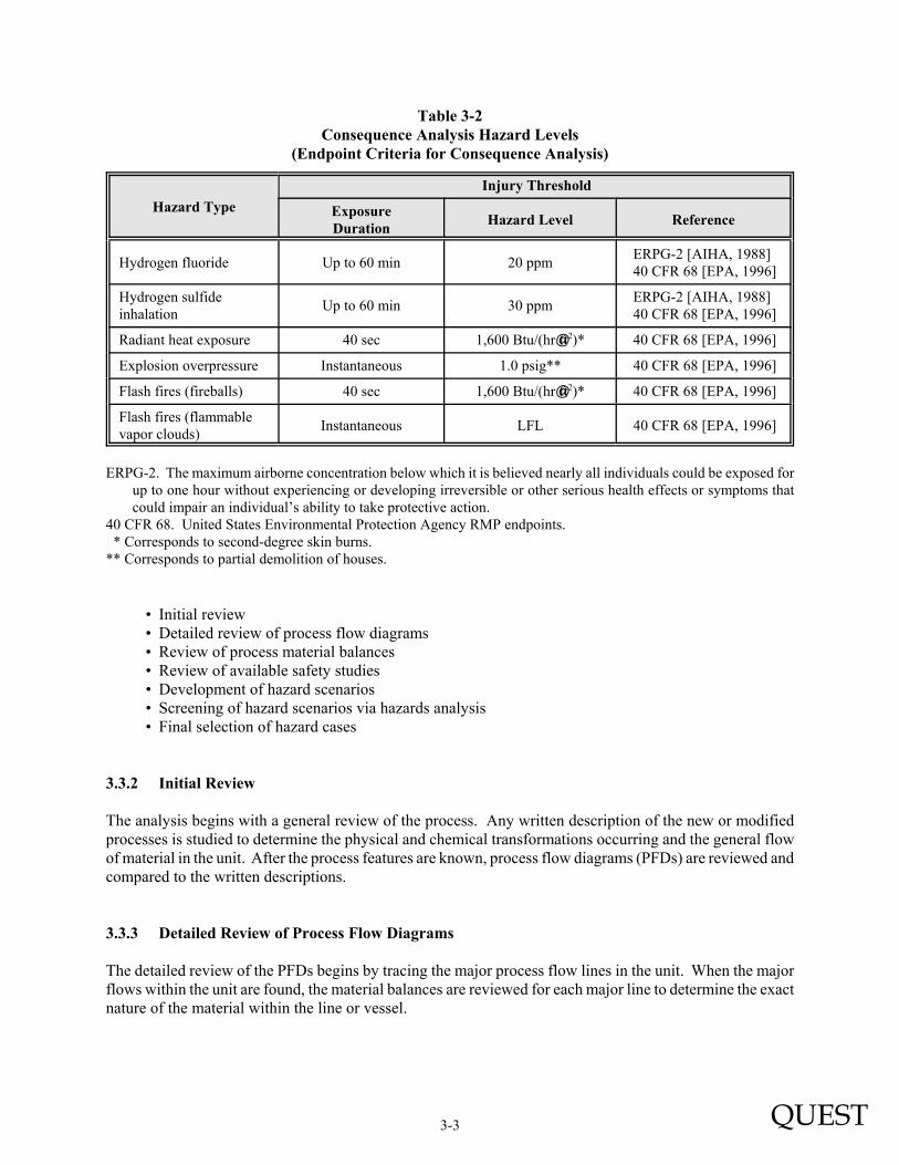
The endpoint hazard criterion defined in this study corresponds to a hazard level which might cause an injury.With this definition, the injury level must be defined for each type of hazard (toxic, radiant heat, or overpres-sure exposure). The South Coast Air Quality Management District has defined equivalent injury levels foreach of the hazards listed. Table 3-2 presents endpoint hazard criteria approved by SCAQMD for this work.

3.3 Selection of Accidental Release Case Studies

3.3.1 Overview of Methodology

The purpose of the hazard case selection methodology is to define the maximum credible hazard scenario foreach unit that might result in an impact to the public. The methodology is developed in seven increments:

QUEST3-3

Table 3-2Consequence Analysis Hazard Levels

(Endpoint Criteria for Consequence Analysis)

Hazard TypeInjury Threshold

ExposureDuration Hazard Level Reference

Hydrogen fluoride Up to 60 min 20 ppm ERPG-2 [AIHA, 1988] 40 CFR 68 [EPA, 1996]

Hydrogen sulfideinhalation Up to 60 min 30 ppm ERPG-2 [AIHA, 1988]

40 CFR 68 [EPA, 1996]

Radiant heat exposure 40 sec 1,600 Btu/(hr@ft2)* 40 CFR 68 [EPA, 1996]

Explosion overpressure Instantaneous 1.0 psig** 40 CFR 68 [EPA, 1996]

Flash fires (fireballs) 40 sec 1,600 Btu/(hr@ft2)* 40 CFR 68 [EPA, 1996]

Flash fires (flammablevapor clouds) Instantaneous LFL 40 CFR 68 [EPA, 1996]

ERPG-2. The maximum airborne concentration below which it is believed nearly all individuals could be exposed forup to one hour without experiencing or developing irreversible or other serious health effects or symptoms thatcould impair an individual’s ability to take protective action.

40 CFR 68. United States Environmental Protection Agency RMP endpoints. * Corresponds to second-degree skin burns.** Corresponds to partial demolition of houses.

• Initial review• Detailed review of process flow diagrams• Review of process material balances• Review of available safety studies• Development of hazard scenarios• Screening of hazard scenarios via hazards analysis• Final selection of hazard cases

3.3.2 Initial Review

The analysis begins with a general review of the process. Any written description of the new or modifiedprocesses is studied to determine the physical and chemical transformations occurring and the general flowof material in the unit. After the process features are known, process flow diagrams (PFDs) are reviewed andcompared to the written descriptions.

3.3.3 Detailed Review of Process Flow Diagrams

The detailed review of the PFDs begins by tracing the major process flow lines in the unit. When the majorflows within the unit are found, the material balances are reviewed for each major line to determine the exactnature of the material within the line or vessel.

QUEST3-4

Each of the major flow lines is taken individually and evaluated to determine the potential for producing amajor hazard if a leak or rupture occurred. At this point in the analysis, a list of potential areas of concernis started; this list is continually refined and added to during the remaining analysis steps.

Several factors are involved in the initial selection of hazard areas:

• Flammability and/or toxic nature of the chemicals• Potential for aerosol formation (releases of streams considerably above their atmospheric boiling

point)• Line size• Normal flow rate in the line• Severity of the process conditions

The factors described above are not weighted equally in the evaluation. The flammability and/or toxic nature,potential for aerosol formation, and process conditions are given more weight than the other factors.

3.3.4 Review of Process Material Balances

Although the process material balances have been reviewed for each major process flow line, they are morethoroughly reviewed during this stage of the analysis to locate points in the process where toxic materialsand/or materials sensitive to detonation are used.

A spreadsheet describing the material balances for the identified hazard locations is begun. The material bal-ance gives the molar flows, the mass flows, and the mole fraction of the components of each process stream.The stream temperature, pressure, and line size are also noted in the spreadsheet. As additional hazard areasare found, their stream summaries are added to the spreadsheet.

3.3.5 Review of Previous Safety Studies

Previous safety studies, including HAZOP reports, “What if?” analyses, safety audits, etc., are reviewed todetermine if all potential hazard areas have been adequately identified. Any potential hazards identified inthese work products are added to the list of potential areas of concern that was started during the detailedreview of the PFDs.

3.3.6 Development of Hazard Scenarios

The list of potential hazard areas developed in the preceding analysis stages is put into a spreadsheet. Thespreadsheet contains the following information:

• Case number• Description of the area where release originates (line, vessel, etc.)• Stream number found on the PFDs• Stream or vessel temperature• Stream or vessel pressure• Assessment of the physical state of the stream (gas, liquid, two-phase)• Total volume of the vessel or the nearest vessel• Liquid volume of the vessel or the nearest vessel

QUEST3-5

• Line size• Normal flow rate of the line or vessel

3.3.7 Initial Screening via Hazard Zone Analysis

The hazard zones resulting from the worst-case releases of similar hazard scenarios are evaluated to determinethe process areas that could release material with a potential for public impact. When performing site-specificconsequence analysis studies, the ability to accurately model the release, dilution, and dispersion of gases andaerosols is important if an accurate assessment of potential exposure is to be attained. For this reason, Questuses a modeling package, CANARY by Quest®, that contains a set of complex models that calculate releaseconditions, initial dilution of the vapor (dependent upon the release characteristics), and the subsequent dis-persion of the vapor introduced into the atmosphere. The models contain algorithms that account for thermo-dynamics, mixture behavior, transient release rates, gas cloud density relative to air, initial velocity of thereleased gas, and heat transfer effects from the surrounding atmosphere and the substrate. The release anddispersion models contained in the QuestFOCUS package (the predecessor to CANARY by Quest) werereviewed in a United States Environmental Protection Agency (EPA) sponsored study [TRC, 1991] and anAmerican Petroleum Institute (API) study [Hanna, Strimaitis, and Chang, 1991]. In both studies, theQuestFOCUS software was evaluated on technical merit (appropriateness of models for specific applications)and on model predictions for specific releases. One conclusion drawn by both studies was that the dispersionsoftware tended to overpredict the extent of the gas cloud travel, thus resulting in too large a cloud whencompared to the test data (i.e., a conservative approach).

A study prepared for the Minerals Management Service [Chang, et al.,1998] reviewed models for use inmodeling routine and accidental releases of flammable and toxic gases. CANARY by Quest received thehighest possible ranking in the science and credibility areas. In addition, the report recommends CANARYby Quest for use when evaluating toxic and flammable gas releases. The specific models (e.g., SLAB) con-tained in the CANARY by Quest software package have also been extensively reviewed. Technical descrip-tions of the CANARY models used in this study are presented in Appendix A.

3.3.8 Final Selection of Hazard Cases

Using the data collected in the hazard area spreadsheet and the initial screening hazard zone calculations, afinal selection of hazard cases is made. These selections generally define the maximum extent of any crediblepotential hazard that could occur in the process area being evaluated.

QUEST4-1

SECTION 4WORST-CASE CONSEQUENCE MODELING RESULTS

The results of the worst-case consequence modeling calculations for the new, modified, and existing unitsare presented in this section. In addition, several hazard zones are overlaid onto the facility map in order todemonstrate the possible public exposure to the defined hazard levels.

4.1 Releases Resulting in the Largest Downwind Hazard Zones

With the completion of the hazard identification and consequence modeling calculations described in Section3 for both the existing and proposed Ultramar configurations, the release from each unit which generates thelargest hazard zone can be identified. These releases are listed in Table 4-1. As can be seen from Table 4-1,most of the proposed modifications do not affect the equipment location where the largest potential releaseoriginates. That is to say, the potential releases which would result in the largest hazard zones are alreadyin place for many of the units. For example, in the Naphtha Hydrotreating Unit (NHT), a rupture of the liquidline leaving the splitter column overhead accumulator results in the largest potential hazard zone (toxic H2Scloud). The modifications to the NHT do not result in release scenarios which could create hazard zoneslarger than those from the splitter column overhead accumulator.

4.2 Description of Potential Hazard Zones

4.2.1 Toxic Vapor Clouds

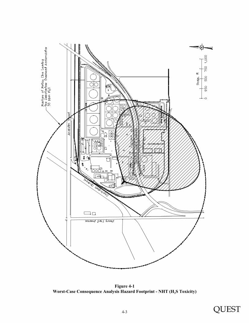
For a potential accident (e.g., pipe break, hole in a vessel, etc.), one particular set of release conditions/atmo-spheric conditions will create the largest potential hazard zone. As an example, consider a rupture of theliquid line leaving the debutanizer overhead accumulator reflux line in the Naphtha Hydrotreater Unit (NHT).This release scenario only exists for post-project conditions because it reflects a change in the operating con-ditions of the unit. In the worst-case release scenario, the material is not ignited, resulting in possible expo-sure to a cloud containing H2S downwind of the release. Under the worst-case atmospheric conditions evalu-ated, the toxic hazard zone (as defined by the ERPG-2 H2S concentration level, 30 ppm) extends 2,150 ftdownwind from the point of release. The hazard “footprint” associated with this event is illustrated in twoways in Figure 4-1. One method presents the hazard zone as a circle which extends 2,150 ft around the pointof release from the debutanizer overhead accumulator. This presentation, referred to as a vulnerability zone,is misleading since everyone within the circle cannot be simultaneously exposed to a 30 ppm H2S level fromany single accident. A more realistic illustration of the potential hazard zone around the release point is givenby the darkened cloud in Figure 4-1. The cloud area illustrates the H2S hazard footprint that would be expect-ed IF a rupture of the reflux line were to occur, AND the wind is blowing at a low speed to the southwest,AND the atmosphere is calm, AND the vapor cloud does not ignite following release.

4.2.2 Vapor Cloud Explosions

One of the possible results of a flammable liquid or gas release is the ignition of flammable vapors, whichcould result in a vapor cloud explosion (VCE). An example of an event tree showing the sequence of eventsthat could lead to a VCE is presented in Figure 4-2. As an example, the 1.0 psig vapor cloud explosionoverpressure hazard footprint following a rupture of the liquid reflux line leaving the debutanizer overhead

QUEST4-2

Table 4-1Potential Accidents Resulting in Maximum Potential Hazard

ProcessUnit/Area

Status of Potential Hazard(E) Existing, (M) Modified,

(N) NewPotential Release (Hazard)

ALKYE Rupture of liquid line leaving acid settler (HF toxicity)

M Rupture of liquid line leaving acid settler (HF toxicity)

BUTAMERE Rupture of liquid line leaving debutanizer accumulator (flash fire)

M Rupture of liquid line leaving debutanizer accumulator (flash fire)

NHTE Rupture of liquid line leaving splitter overhead accumulator (flash

fire)

N Rupture of liquid reflux line leaving debutanizer overhead accumulator (H2S toxicity)

FGTUE Rupture of fuel gas inlet line (H2S toxicity)

M Rupture of fuel gas inlet line (H2S toxicity)

LER1E Rupture of sour gas line leaving debutanizer accumulator

(H2S toxicity)

M Rupture of liquid line leaving debutanizer accumulator(H2S toxicity)

LER2E Rupture of liquid line leaving debutanizer accumulator

(H2S toxicity)

M Rupture of liquid line leaving debutanizer accumulator(H2S toxicity)

MEROXE Rupture of liquid line leaving caustic prewash (flash fire)

N Rupture of liquid line leaving caustic prewash (flash fire)

TANKE Tank 95-TK-1 recovered oil tank fire (fire radiation)

M Tank 95-TK-1 recovered oil tank fire (fire radiation)

LPG(C3 STORAGE)

E BLEVE of 2,000 barrel LPG bullet (fire radiation)

N BLEVE of 4,000 barrel LPG bullet (fire radiation)

LPG(C4 STORAGE)

E BLEVE of 4,760 barrel butane sphere (fire radiation)

N BLEVE of 5,000 barrel butane sphere (fire radiation)

HOHE Rupture of fuel gas line (flash fire)

M Rupture of fuel gas line (flash fire)

BOILER N Rupture of fuel gas line (flash fire)

AQNH3 TANKE Rupture of liquid line from tank (NH3 toxicity)

N Rupture of liquid line from tank (NH3 toxicity)

accumulator in the NHT is presented in Figure 4-3. This hazard extends 790 ft from the process area whereflammable vapors are confined. For explosions that originate in a process area, the hazard footprint isidentical to the vulnerability zone.

QUEST4-3

Figure 4-1Worst-Case Consequence Analysis Hazard Footprint - NHT (H2S Toxicity)

QUEST4-4

Out

com

e

Imm

edia

te Ig

nitio

nPo

ol/T

orch

Fire

Fire

Flas

h Fi

re

Rup

ture

Del

ayed

Igni

tion

2 in

< d

< 6

inV

apor

Clo

ud E

xplo

sion

VC

E

No

Igni

tion

Toxi

c C

loud

Imm

edia

te Ig

nitio

nPo

ol/T

orch

Fire

Rel

ease

of L

iqui

d or

Li

quef

ied

Gas

from

Hig

h-Pr

essu

re P

ipin

g

Fire

Flas

h Fi

re

Maj

or L

eak

Del

ayed

Igni

tion

Pipe

Dia

met

er '

6 in

0.25

in <

d <

6 in

Vap

or C

loud

Exp

losi

onV

CE

No

Igni

tion

Toxi

c C

loud

Imm

edia

te Ig

nitio

nPo

ol/T

orch

Fire

Fire

Flas

h Fi

re

Min

or L

eak

Del

ayed

Igni

tion

d <

0.25

inV

apor

Clo

ud E

xplo

sion

VC

E

No

Igni

tion

Toxi

c C

loud

Figure 4-2Event Tree for a Flammable/Toxic Release

QUEST4-5

Figure 4-3Worst-Case Consequence Analysis Hazard Footprint - NHT (Explosion Overpressure)

QUEST4-6

4.2.3 Flash Fires

A release of flammable fluid, if not ignited immediately, will create a vapor cloud that travels downwind anddisperses. The extent of the flammable zone is defined by the lower flammable limit (LFL). If the flammablecloud is ignited after reaching its full extent, the largest possible flash fire will result. The hazard footprintfor a rupture of the liquid reflux line leaving the debutanizer overhead accumulator in the NHT is shown inFigure 4-4. This hazard extends 1,090 ft downwind from the point of release. The flash fire hazard zone issimilar to the toxic hazard zone in that the vulnerability zone (circle) covers a much larger area than the actualvapor cloud (the hazard footprint represented by the shaded area).

4.2.4 Fire Radiation

The most significant fire radiation hazards that might occur are torch fires from liquefied gas releases. Unlikethe dispersion calculations, the worst-case atmospheric conditions for torch fire radiation calculations occurwhen the winds are high, allowing the flame to “bend” downwind. The largest potential pool fire hazardzones are due to atmospheric storage tank fires. Examples of radiant hazard zones for an immediately ignitedrupture of the liquid line leaving the debutanizer overhead accumulator in the NHT, and tank fires from thecurrent and proposed locations of the recovered oil tanks are presented in Figure 4-5.

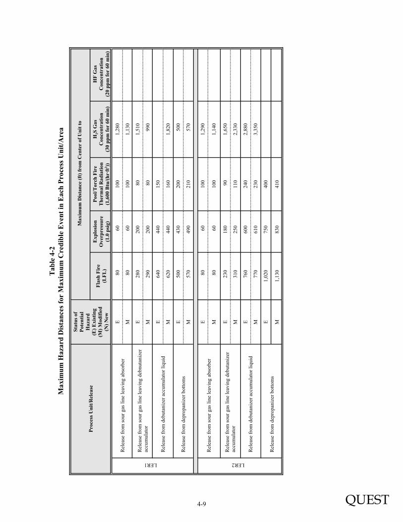
4.3 Summary of Maximum Hazard Zones

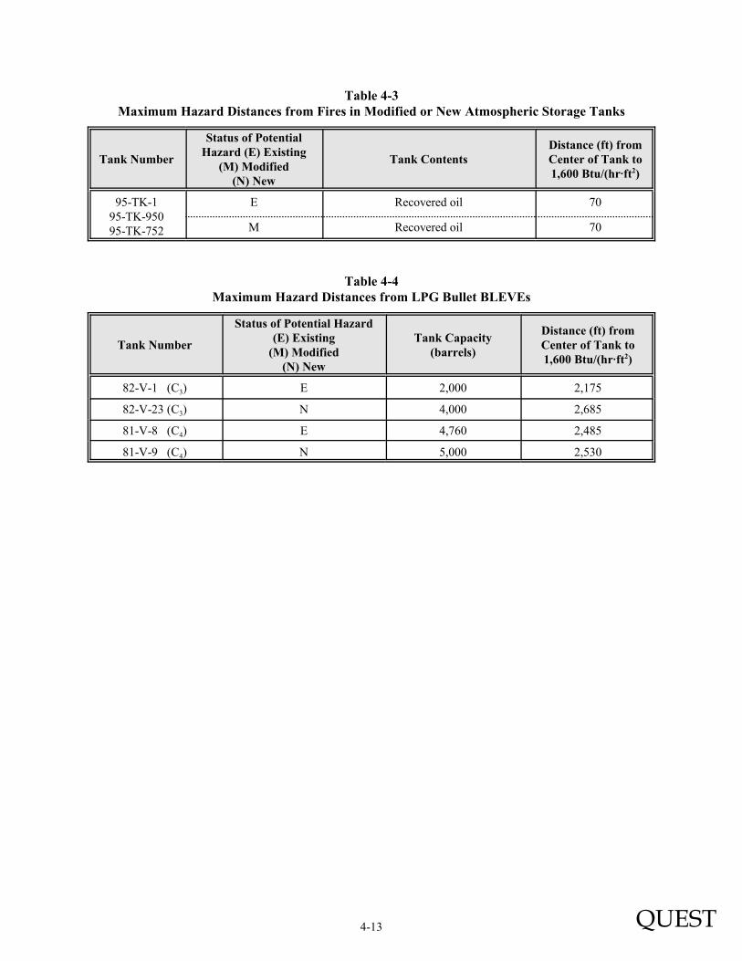
Table 4-2 presents a listing of the type and size of potential hazards which dominate each of the units eval-uated. Note that for each unit, the status is defined as E, M, or N (existing, modified, or new). The largesthazards are listed for releases from the existing units and the units after the proposed modifications. Thehazards resulting from storage tank fires are listed in Table 4-3. The most significant hazards associated withthe pressurized storage tanks (LPG bullets) are BLEVEs. The distance to the thermal radiation endpoint foreach size of LPG storage bullet is listed in Table 4-4.

Overall, the proposed additions and modifications result in a limited number of increases in the size of poten-tial hazards. Many of the increases in hazard zones are restricted to Ultramar’s property. The addition of twonew LPG bullets created the largest increase in radiant off-site hazards, but the effects of bullet BLEVEs (rareevents) are constrained to off-site industrial areas.

QUEST4-7

Figure 4-4Worst-Case Consequence Analysis Hazard Footprint - NHT (Flash Fire)

QUEST4-8

Figure 4-5Worst-Case Consequence Analysis Hazard Footprints - NHT, TANK (Fire Radiation)

QUEST4-9

Tab

le 4

-2M

axim

um H

azar

d D

ista

nces

for

Max

imum

Cre

dibl

e E

vent

in E

ach

Proc

ess U

nit/A

rea

Proc

ess U

nit/R

elea

se

Stat

us o

fPo

tent

ial

Haz

ard

(E) E

xist

ing

(M) M

odifi

ed(N

) New

Max

imum

Dis

tanc

e (f

t) fr

om C

ente

r of

Uni

t to

Flas

h Fi

re(L

FL)

Exp

losi

onO

verp

ress

ure

(1.0

psi

g)

Pool

/Tor

ch F

ire

The

rmal

Rad

iatio

n(1

,600

Btu

/(hr@

ft2 ))

H2S

Gas

Con

cent

ratio

n(3

0 pp

m fo

r 60

min

)

HF

Gas

Con

cent

ratio

n(2

0 pp

m fo

r 60

min

)

Rel

ease

from

sour

gas

line

leav

ing

abso

rber

E

80

6

010

01,

280

M

80

6

010

01,

130

Rel

ease

from

sour

gas

line

leav

ing

debn

utan

izer

accu

mul

ator

E

280

20

0 8

01,

510

M

290

20

0 8

0

990

Rel

ease

from

deb

utan

izer

acc

umul

ator

liqu

idE

64

0

440

150

M

620

44

016

01,

820

Rel

ease

from

dep

ropa

nize

r bot

tom

sE

50

0

430

200

50

0

M

570

49

021

0

570

Rel

ease

from

sour

gas

line

leav

ing

abso

rber

E

80

6

010

01,

290

M

80

6

010

01,

140

Rel

ease

from

sour

gas

line

leav

ing

debu

tani

zer

accu

mul

ator

E

230

18

0 9

01,

650

M

310

25

011

02,

330

Rel

ease

from

deb

utan

izer

acc

umul

ator

liqu

idE

76

0

600

240

2,88

0

M

770

61

023

03,

350

Rel

ease

from

dep

ropa

nize

r bot

tom

sE

1,02

0

750

400

M1,

130

83

041

0

LER1 LER2

QUEST4-10

NHTT

able

4-2

Max

imum

Haz

ard

Dis

tanc

es fo

r M

axim

um C

redi

ble

Eve

nt in

Eac

h Pr

oces

s Uni

t/Are

a(C

ontin

ued)

Proc

ess U

nit/R

elea

se

Stat

us o

fPo

tent

ial

Haz

ard

(E) E

xist

ing

(M) M

odifi

ed(N

) New

Max

imum

Dis

tanc

e (f

t) fr

om C

ente

r of

Uni

t to

Flas

h Fi

re(L

FL)

Exp

losi

onO

verp

ress

ure

(1.0

psi

g)

Pool

/Tor

ch F

ire

The

rmal

Rad

iatio

n(1

,600

Btu

/(hr@

ft2 ))

H2S

Gas

Con

cent

ratio

n(3

0 pp

m fo

r 60

min

)

HF

Gas

Con

cent

ratio

n(2

0 pp

m fo

r 60

min

)

Rel

ease

from

reac

tor e

fflu

ent l

ine

E

230

17

036

01,

320

M

230

18

035

0

880

Rel

ease

from

strip

per b

otto

ms

E1,

200

1,01

048

0

M1,

290

1,09

047

0

Rel

ease

from

nap

htha

strip

per b

otto

ms

E1,

380

99

059

0

M1,

300

95

059

0

Rel

ease

from

split

ter o

verh

ead

accu

mul

ator

E1,

940

1,22

045

0

M1,

770

1,16

047

0

Rel

ease

of s

our g

as fr

om st

rippe

r ove

rhea

dac

cum

ulat

orE

9

0

60

110

1,53

0

M

80

6

010

01,

310

Rel

ease

from

deb

utan

izer

reflu

x lin

eN

1,09

0

790

350

2,15

0

Rel

ease

of L

PG fr

om c

aust

ic p

rew

ash

vess

elE

1,03

0

620

170

M1,

270

82

022

0

MEROX

QUEST4-11

FGTUT

able

4-2

Max

imum

Haz

ard

Dis

tanc

es fo

r M

axim

um C

redi

ble

Eve

nt in

Eac

h Pr

oces

s Uni

t/Are

a(C

ontin

ued)

Proc

ess U

nit/R

elea

se

Stat

us o

fPo

tent

ial

Haz

ard

(E) E

xist

ing

(M) M

odifi

ed(N

) New

Max

imum

Dis

tanc

e (f

t) fr

om C

ente

r of

Uni

t to

Flas

h Fi

re(L

FL)

Exp

losi

onO

verp

ress

ure

(1.0

psi

g)

Pool

/Tor

ch F

ire

The

rmal

Rad

iatio

n(1

,600

Btu

/(hr@

ft2 ))

H2S

Gas

Con

cent

ratio

n(3

0 pp

m fo

r 60

min

)

HF

Gas

Con

cent

ratio

n(2

0 pp

m fo

r 60

min

)

Rel

ease

from

settl

er a

cid

outle

tE

25,2

40

M23

,250

Rel

ease

from

ole

fin fe

ed to

reac

tor

E1,

960

1,30

036

0

M2,

060

1,49

047

0

Rel

ease

from

reac

tor o

utle

tE

9

0

110

190

24,7

90

M

40

5

013

019

,990

Rel

ease

from

isos

tripp

er b

otto

ms

E1,

320

1,06

077

0

M1,

380

1,10

077

0

Rel

ease

from

dep

ropa

nize

r rec

eive

r out

let

E1,

090

91

044

0

M1,

170

97

044

0

Rel

ease

from

fuel

gas

inle

tE

12

0

90

150

210

M

120

9

015

021

0

Rel

ease

from

feed

surg

e dr

umE

1,18

0

830

400

M1,

280

89

041

0

Rel

ease

from

stab

ilize

r bot

tom

sE

83

0

670

270

M

960

75

029

0

Rel

ease

from

deb

utan

izer

ove

rhea

d ac

cum

ulat

orE

1,75

01,

400

595

M1,

960

1,57

059

0

ALKY BUTAMER

QUEST4-12

LPG(C4 STORAGE)

LPG(C3 STORAGE) BOILER AQNH3 TANK

Tab

le 4

-2M

axim

um H

azar

d D

ista

nces

for

Max

imum

Cre

dibl

e E

vent

in E

ach

Proc

ess U

nit/A

rea

(Con

tinue

d)

Proc

ess U

nit/R

elea

se

Stat

us o

fPo

tent

ial

Haz

ard

(E) E

xist

ing

(M) M

odifi

ed(N

) New

Max

imum

Dis

tanc

e (f

t) fr

om C

ente

r of

Uni

t to

Flas

h Fi

re(L

FL)

Exp

losi

onO

verp

ress

ure

(1.0

psi

g)

Pool

/Tor

ch F

ire

The

rmal

Rad

iatio

n(1

,600

Btu

/(hr@

ft2 ))

H2S

Gas

Con

cent

ratio

n(3

0 pp

m fo

r 60

min

)

HF

Gas

Con

cent

ratio

n(2

0 pp

m fo

r 60

min

)

Rel

ease

from

but

ane

sphe

re

E2,

450

5,49

02,

485

M2,

510

7,88

02,

530

Rel

ease

from

pro

pane

bul

let

E2,

010

5,30

02,

175

M2,

250

5,64

02,

685

Rel

ease

from

boi

ler f

uel g

as li

neN

9

0

70

8

0

Rel

ease

from

aqu

eous

NH

3 tan

k

E21

0

M30

0

Rel

ease

from

fuel

gas

line

E

80

6

0 7

0

M

90

7

0 8

0

HOH

QUEST4-13

Table 4-3Maximum Hazard Distances from Fires in Modified or New Atmospheric Storage Tanks

Tank Number

Status of PotentialHazard (E) Existing

(M) Modified(N) New

Tank ContentsDistance (ft) fromCenter of Tank to1,600 Btu/(hr@ft2)

95-TK-195-TK-95095-TK-752

E Recovered oil 70

M Recovered oil 70

Table 4-4Maximum Hazard Distances from LPG Bullet BLEVEs

Tank Number

Status of Potential Hazard(E) Existing

(M) Modified(N) New

Tank Capacity(barrels)

Distance (ft) fromCenter of Tank to1,600 Btu/(hr@ft2)

82-V-1 (C3) E 2,000 2,175

82-V-23 (C3) N 4,000 2,685

81-V-8 (C4) E 4,760 2,485

81-V-9 (C4) N 5,000 2,530

QUEST5-1

SECTION 5CONCLUSIONS

The primary conclusion that can be drawn from the worst-case consequence modeling results is that for thenew process unit, the proposed modifications to existing process units and the additions to storage do notresult in significantly larger potential hazard zones than those posed by the existing Ultramar Refineryconfiguration. This result is primarily due to the nature of many of the modifications, which can best bedescribed in the following manner.

• Modification of a unit such that the largest potential hazard is changed only slightly (e.g., ButamerUnit).

• Addition of equivalent equipment such that the potential hazards are essentially the same as thosewhich already exist (e.g., the Merox Unit).

• Relocating products within the refinery property (e.g., relocating atmospheric storage tanks, the haz-ards associated with atmospheric storage of liquid hydrocarbons remain the same and remain on-site).

With the maximum hazard zones defined for each release, the units can be divided into three categories,dependent on their potential to impact the public. The categories are defined as:

• Units with no potential pre- or post-project off-site impacts (hazard zones are contained on-site).HOHBOILERFGTUTANKAQNH3 TANK

• Units with potential pre- or post-project off-site impacts, but post-project impacts are no larger thanpre-project (existing) impacts.

ALKY• Units with potential off-site impacts. Post-project impacts are larger than pre-project impacts.

LER1LER2NHTMEROXBUTAMERLPG (C4 STORAGE)LPG (C3 STORAGE)

Two specific conclusions can be drawn from a review of the worst-case consequence modeling results. First,for those units where post-project off-site impacts are larger then pre-project off-site impacts, none of theincreased hazard zones reach a residential area. All are confined to the industrial area near the Ultramarrefinery complex. The worst-case comparison is only valid for the maximum impact distances. All otherpotential releases are smaller and, in many cases, there is no difference between the pre- and post-projectimpacts.

The second specific conclusion that can be drawn from the study is that the modifications to the AlkylationUnit (ALKY) produce a significant reduction in the potential worst-case impact following a release of

QUEST5-2

hydrofluoric acid bearing fluids. The implementation of the ReVAP process, with its use of the acid additivewhich reduces the volatility of the acid phase, results in an 7.9% reduction in the maximum hazard distance.Similar reductions in the downwind travel of HF-bearing clouds will be found for all potential acid releasesin the proposed alkylation unit.

None of the modified or new units creates a new hazard that could extend into residential areas. With theexception of the Alkylation Unit; all off-site hazards are confined to industrial areas surrounding the facility.The potential impacts from the Alkylation Unit are significantly reduced with the use of the ReVAP process.Although there is still the potential for a release to extend off-site into residential areas, the area potentiallyexposed will be reduced with the project modifications. It should be kept in mind that for the worst-casescenario to occur, the following conditions must be met.

(1) A full rupture of the line occurs.(2) The release does not ignite within minutes of the rupture.(3) The wind speed is low (less than 3 mph).(4) The atmosphere is calm.

This sequence of events is highly unlikely and only results in an off-site hazard (toxic or flammable vapordispersion) for a limited number of potential releases. The other hazards that were found to be larger afterthe proposed additions and modifications were a BLEVE of one of the new LPG bullets. These events,which are not affected by the above considerations, are also very rare.

QUEST6-1

SECTION 6REFERENCES

AIHA (1988), Emergency Response Planning Guidelines. American Industrial Hygiene Association, Akron, Ohio,1988.

Chang, Joseph C., Mark E. Fernau, Joseph S. Scire, and David G. Strimatis (1998), A Critical Review of FourTypes of Air Quality Models Pertinent to MMS Regulatory and Environmental Assessment Missions.Mineral Management Service, Gulf of Mexico OCS Region, U.S. Department of the Interior, NewOrleans, November, 1998.

EPA (1996), Accidental Release Prevention Requirements: Risk Management Programs Under the Clean AirAct, Section 112(r)(7). Environmental Protection Agency, 40 CFR Part 68, 1996.

Hanna, S. R., D. G. Strimaitis, and J. C. Chang (1991), Hazard Response Modeling Uncertainty (A Quantita-tive Method), Volume II, Evaluation of Commonly-Used Hazardous Gas Dispersion Models. Studycosponsored by the Air Force Engineering and Services Center, Tyndall Air Force Base, Florida, and theAmerican Petroleum Institute; performed by Sigma Research Corporation, Westford, Massachusetts,September, 1991.

TRC (1991), Evaluation of Dense Gas Simulation Models. Prepared for the U.S. Environmental ProtectionAgency by TRC Environmental Consultants, Inc., East Hartford, Connecticut 06108, EPA Contract No.68-02-4399, May, 1991.

QUEST7-1

SECTION 7GLOSSARY

The following definitions are intended to apply to Consequence Analysis and Quantitative Risk Analysisstudies of facilities that produce, process, store, or transport hazardous materials. Due to the limited scopeof such studies, some of these definitions are more narrow than the common definitions.

ACCIDENT. An unplanned event that interrupts the normal progress of an activity and has undesirable conse-quences, and is preceded by an unsafe act and/or an unsafe condition.

ACCIDENT EVENT SEQUENCE. A specific series of unplanned events that has specific undesirable conse-quences (e.g., a pipe ruptures, allowing flammable gas to escape; the gas forms a flammable vaporcloud that ignites after some delay, resulting in a flash fire).

ACCIDENT SCENARIO. The detailed description of an accident event sequence.

AIR DISPERSION MODELING. The use of mathematical equations (models) to predict the rate at which vaporsor gases released into the air will be diluted (dispersed) by the air. The purpose of air dispersionmodeling is to predict the extent of potentially toxic or flammable gas concentrations, in air, bycalculating the change in concentration of the vapor or gas in the air as a function of distance fromthe source of the vapor or gas.

BLAST WAVE. An atmospheric pressure pulse created by an explosion.

BLEVE (Boiling Liquid–Expanding Vapor Explosion). The sudden, catastrophic failure of a pressure vesselat a time when its liquid contents are well superheated. (BLEVE is normally associated with the rup-ture, due to fire impingement, of pressure vessels containing liquefied gases.)

CONDITIONAL PROBABILITY. The probability of occurrence of an event, given that one or more precursorevents have occurred (e.g., the probability of ignition of an existing vapor cloud).

CONSEQUENCES. The expected results of an incident outcome.

CONSEQUENCE ANALYSIS. Selection and definition of specific accident event sequences, coupled with con-sequence modeling.

CONSEQUENCE MODELING. The use of mathematical models to predict the potential extent of specific hazardzones or effect zones that would result from specific accident event sequences.

DEFLAGRATION. See explosion.

DETONATION. See explosion.

EFFECT ZONE. The area over which the airborne gas concentration, radiant heat flux, or blast wave overpres-sure is predicted to equal or exceed some specified value. In contrast to a hazard zone, the endpointfor an effect zone need not be capable of producing injuries or damage.

QUEST7-2

ENDPOINT. The specified value of airborne gas concentration, radiant heat flux, or blast wave overpressureused to define the outer boundary of an effect zone or hazard zone. Endpoints typically correspondto specific levels of concern (e.g., IDLH, LFL, onset of fatality, 50% mortality, odor threshold, etc.).

EVENT TREE. A diagram that illustrates accident event sequences. It begins with an initiating event (e.g., arelease of hydrogen sulfide gas), passes through one or more intermediate events (e.g., ignition orno ignition), resulting in two or more incident outcomes (e.g., flash fire or toxic vapor cloud).

EXPLOSION. A rapid release of energy, resulting in production of a blast wave. There are two common typesof explosions—physical explosions (sudden releases of gas or liquefied gas from pressurized con-tainers) and chemical explosions (rapid chemical reactions, including rapid combustion). Chemicalexplosions can be further subdivided into deflagrations and detonations. In a deflagration, thevelocity of the blast wave is lower than the speed of sound in the reactants. In a detonation, thevelocity of the blast wave exceeds the speed of sound in the reactants. For a given mass of identicalreactants, a detonation is capable of producing more damage than a deflagration. Solid and liquidexplosives, such as dynamite and nitroglycerine, typically detonate, whereas vapor cloud explosionsare nearly always deflagrations.

FIRE RADIATION. See thermal radiation.

FLAMMABLE VAPOR CLOUD. A vapor cloud consisting of flammable gas and air, within which the gas con-centration equals or exceeds its lower flammable limit.

FLASH FIRE. Transient combustion of a flammable vapor cloud.

HAZARD. A chemical or physical condition that presents a potential for causing injuries or illness to people,damage to property, or damage to the environment.

HAZARD ZONE. The area over which a given incident outcome is capable of producing undesirable conse-quences (e.g., skin burns) that are equal to or greater than some specified injury or damage level (e.g.,second-degree skin burns). (Sometimes referred to as a “hazard footprint.”)

INCIDENT OUTCOME. The result of an accident event sequence. The incident outcomes of interest in a typicalstudy are toxic vapor clouds; fires (flash fire, torch fire, pool fire, or fireball); and explosions (con-fined, unconfined, or physical).

INITIATING EVENT. The first event in an accident event sequence. Typically a failure of containment (e.g.,gasket failure, corrosion hole in a pipe, hose rupture, etc.).

INTERMEDIATE EVENT. An event that propagates or mitigates the previous event in an accident eventsequence (e.g., operator fails to respond to an alarm, thus allowing a release to continue; excess flowvalve closes, thus stopping the release).

ISOPLETH. The locus of points at which a given variable has a constant value. In consequence modeling, thevariable can be airborne gas concentration, radiant heat flux, or blast wave overpressure. The valueof the variable is equal to the specified endpoint. The area bounded by an isopleth is an effect zone.

LOWER FLAMMABLE LIMIT. The lowest concentration of flammable gas in air that will support flame propa-gation.

QUEST7-3

MISSILES. See shrapnel.

POOL FIRE. Continuous combustion of the flammable gas emanating from a pool of liquid.

QUANTITATIVE RISK ANALYSIS. The development of a quantitative estimate of risk based on engineeringevaluation and mathematical techniques for combining estimates of incident consequences andfrequencies.

RISK. A measure of economic loss or human injury in terms of both the incident likelihood and themagnitude of the loss or injury.

RISK ASSESSMENT. The process by which the results of a risk analysis are used to make decisions, eitherthrough relative ranking of risk reduction strategies or through comparison with risk targets.

SHRAPNEL. Solid objects projected outward from the source of an explosion. Sometimes referred to asmissiles or projectiles.

SUPERHEATED LIQUID. A liquid at a temperature greater than its atmospheric pressure boiling point.

THERMAL RADIATION. The transfer of heat by electromagnetic waves. This is how heat is transferred fromflames to an object or person not in contact with or immediately adjacent to the flames. This is alsohow heat is transferred from the sun to the earth.

TORCH FIRE. Continuous combustion of a flammable fluid that is being released with considerable momen-tum.

TOXIC. Describes a material with median lethal doses and/or median lethal concentrations listed in OSHA29 CFR 1910.1200, Appendix A.

TOXIC VAPOR CLOUD. A vapor cloud consisting of toxic gas and air, within which the gas concentrationequals or exceeds a concentration that could be harmful to humans exposed for a specific time.

VAPOR CLOUD. A volume of gas/air mixture within which the gas concentration equals or exceeds somespecified or defined concentration limit.

VAPOR CLOUD EXPLOSION. Extremely rapid combustion of a flammable vapor cloud, resulting in a blastwave.

VULNERABILITY ZONE. The area within the circle created by rotating a hazard zone around its point of origin.Any point within that circle could, under some set of circumstances, be exposed to a hazard level thatequals or exceeds the endpoint used to define the hazard zone. However, except for accidents thatproduce circular hazard zones (e.g., BLEVEs and confined explosions), only a portion of the areawithin the vulnerability zone can be affected by a single accident.

QUEST7-4

API American Petroleum Institute

BLEVE Boiling Liquid–Expanding Vapor Explosion

CCPS Center for Chemical Process Safety

DOT Department of Transportation

EPA Environmental Protection Agency

ESD Emergency Shut Down

FTA Fault Tree Analysis

IDLH Immediately Dangerous to Life or Health

LFL Lower Flammable Limit

LPG Liquefied Petroleum Gas

NFPA National Fire Protection Association

OREDA Offshore Reliability Data

psig Pounds per square inch, gauge

QRA Quantitative Risk Analysis

RMP Risk Management Plan

STEL Short-Term Exposure Limit

TNO Netherlands Organization of Applied Scientific Research (Nederlandse Organisatie voortoegepest-natuurwetenschallelijk onderzoek)

TNT Trinitrotoluene

USCB United States Census Bureau

USNRC United States Nuclear Regulatory Commission

QUESTA-1

APPENDIX ACANARY BY QUEST® MODEL DESCRIPTIONS

The following model descriptions are taken from the CANARY by Quest User Manual.

Section A Engineering PropertiesSection B Pool Fire Radiation ModelSection C Torch Fire and Flare Radiation ModelSection D Fireball ModelSection E Fluid Release ModelSection F Momentum Jet Dispersion ModelSection G Heavy Gas Dispersion ModelSection I Vapor Cloud Explosion Model

CANARY by Quest User’s Manual Section A. Engineering Properties

July, 2003 Section A - Page 1

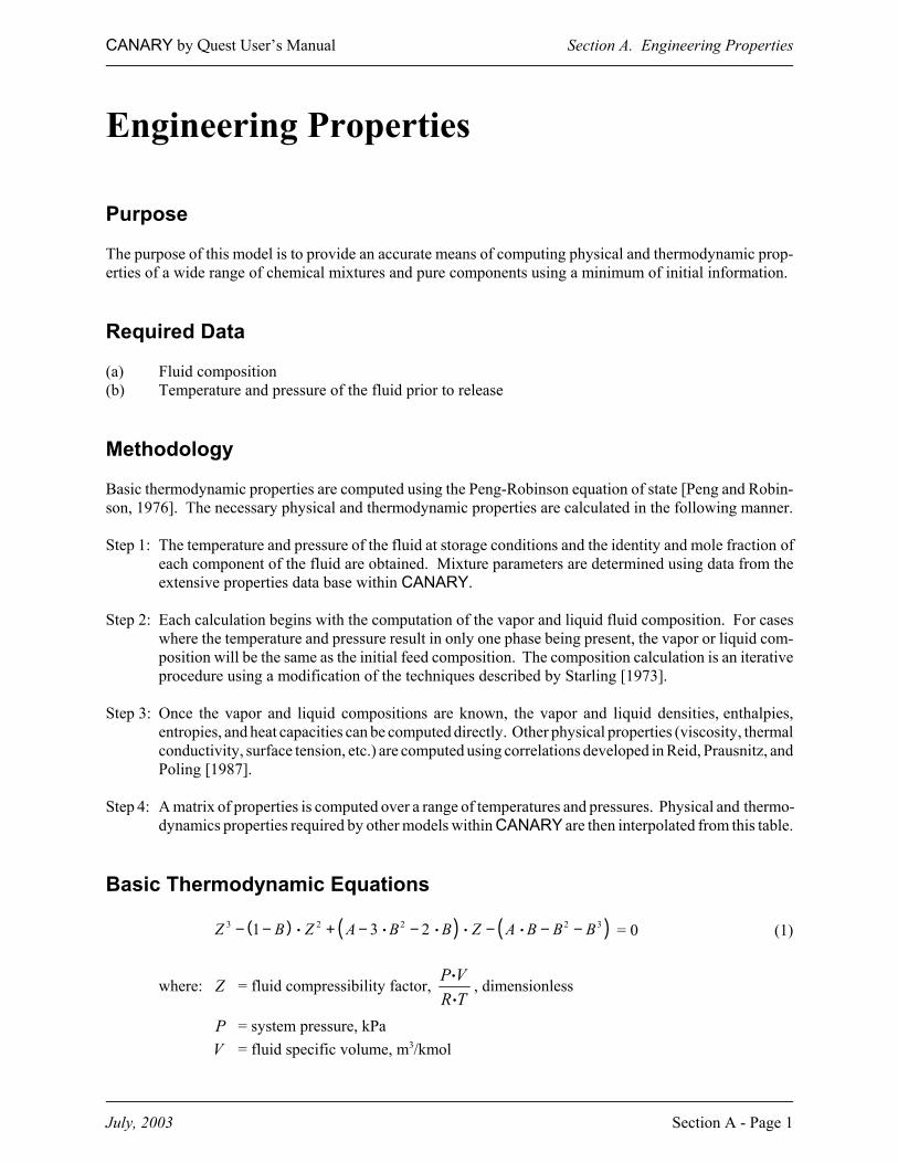
Engineering Properties

Purpose

The purpose of this model is to provide an accurate means of computing physical and thermodynamic prop-erties of a wide range of chemical mixtures and pure components using a minimum of initial information.

Required Data

(a) Fluid composition(b) Temperature and pressure of the fluid prior to release

Methodology

Basic thermodynamic properties are computed using the Peng-Robinson equation of state [Peng and Robin-son, 1976]. The necessary physical and thermodynamic properties are calculated in the following manner.

Step 1: The temperature and pressure of the fluid at storage conditions and the identity and mole fraction ofeach component of the fluid are obtained. Mixture parameters are determined using data from theextensive properties data base within CANARY.

Step 2: Each calculation begins with the computation of the vapor and liquid fluid composition. For caseswhere the temperature and pressure result in only one phase being present, the vapor or liquid com-position will be the same as the initial feed composition. The composition calculation is an iterativeprocedure using a modification of the techniques described by Starling [1973].

Step 3: Once the vapor and liquid compositions are known, the vapor and liquid densities, enthalpies,entropies, and heat capacities can be computed directly. Other physical properties (viscosity, thermalconductivity, surface tension, etc.) are computed using correlations developed in Reid, Prausnitz, andPoling [1987].

Step 4: A matrix of properties is computed over a range of temperatures and pressures. Physical and thermo-dynamics properties required by other models within CANARY are then interpolated from this table.

Basic Thermodynamic Equations

= 0 (1)( ) ( ) ( )3 2 2 2 31 3 2Z B Z A B B Z A B B B− − + − − − − −i i i i i

where: = fluid compressibility factor, , dimensionlessZ P VR Ti

i

= system pressure, kPaP= fluid specific volume, m3/kmolV



= gas constant, 8.314 m3 kPa/(kmol K)R i i

= absolute temperature, KT

= A 2 2

a PR T

i

i

= a2 2

0.45724c

R TP

αi

i i

= α ( )20.51 1 rm T + − i

= m 20.37464 1.54226 0.26992ω ω+ −i i

= acentric factorω

=rTc

TT

= pseudo-critical temperature, KcT= pseudo-critical pressure, kPacP

= B b PR Ti

i

= b 0.0778 c

c

TRP

i i

= (2)H 20

o P P dH R T P TT

ρ

ρ

ρρ ρ

∂ + − + − ∂

⌠⌡

i i i

where: = enthalpy of fluid at system conditions, kJ/kgH= enthalpy of ideal gas at system temperature, kJ/kgoH

= (3)S ( ) 20

lno P dS R R T RT

ρ

ρ

ρρ ρρ

∂ − + − ∂

⌠⌡

i i i i i

where: = entropy of fluid at system conditions, kJ/(kg K)S i

= entropy of ideal gas at system temperature, kJ/(kg K)oS i

= (4)ln io

i

fR Tf

i i ( ) ( )o oi i i iH H T S S − − − i

where: = fugacity of component kPaif ,i

= standard state reference fugacity, kPaoif



References

Peng, D., and D. B. Robinson, “New Two-Constant Equation of State.” Industrial Engineering ChemistryFundamentals, Vol. 15, No. 59, 1976.

Reid, R. C., J. M. Prausnitz, and B. E. Poling, The Properties of Gases and Liquids (Fourth Edition).McGraw-Hill Book Company, New York, New York, 1987.

Starling, K. E., Fluid Thermodynamic Properties for Light Petroleum Systems. Gulf Publishing Company,Houston, Texas, 1973.

CANARY by Quest User’s Manual Section B. Pool Fire Radiation Model

July, 2003 Section B - Page 1

Pool Fire Radiation Model

Purpose

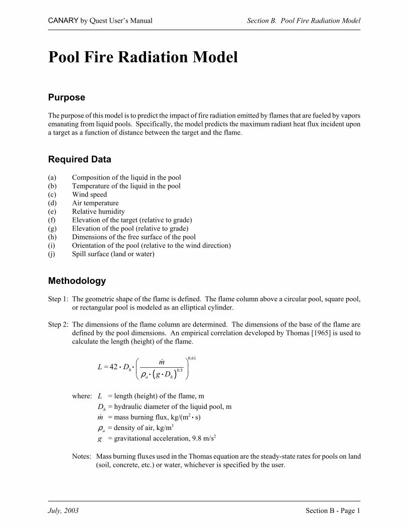
The purpose of this model is to predict the impact of fire radiation emitted by flames that are fueled by vaporsemanating from liquid pools. Specifically, the model predicts the maximum radiant heat flux incident upona target as a function of distance between the target and the flame.

Required Data

(a) Composition of the liquid in the pool(b) Temperature of the liquid in the pool(c) Wind speed(d) Air temperature(e) Relative humidity(f) Elevation of the target (relative to grade)(g) Elevation of the pool (relative to grade)(h) Dimensions of the free surface of the pool(i) Orientation of the pool (relative to the wind direction)(j) Spill surface (land or water)

Methodology

Step 1: The geometric shape of the flame is defined. The flame column above a circular pool, square pool,or rectangular pool is modeled as an elliptical cylinder.

Step 2: The dimensions of the flame column are determined. The dimensions of the base of the flame aredefined by the pool dimensions. An empirical correlation developed by Thomas [1965] is used tocalculate the length (height) of the flame.

=L( )

0.61

0.542 ha h

mDg Dρ

i ii i

where: = length (height) of the flame, mL= hydraulic diameter of the liquid pool, mhD= mass burning flux, kg/(m2 s)m i

= density of air, kg/m3aρ

= gravitational acceleration, 9.8 m/s2g

Notes: Mass burning fluxes used in the Thomas equation are the steady-state rates for pools on land(soil, concrete, etc.) or water, whichever is specified by the user.



For pool fires with hydraulic diameters greater than 100 m, the flame length, is set equal,Lto the length calculated for 100 m.hD =

Step 3: The angle to which the flame is bent from vertical by the wind is calculated using an empirical( )Φcorrelation developed by Welker and Sliepcevich [1970].

= tan( )cos ( )

ΦΦ

0.70.07 0.62

3.2 h a v

a h a

D u ug D

ρ ρµ ρ

−

i ii i i

i

where: = angle the flame tilts from vertical, degreesΦ= wind speed, m/su = viscosity of air, kg/(m s)aµ i

= density of fuel vapor, kg/m3vρ

Step 4: The increase in the downwind dimension of the base of the flame (flame drag) is calculated using ageneralized form of the empirical correlation Moorhouse [1982] developed for large circular poolfires.

= wD0.0692

1.5 xx

uDg D

i ii

where: = downwind dimension of base of tilted flame, mwD= downwind dimension of the pool, mxD

Step 5: The flame is divided into two zones: a clear zone in which the flame is not obscured by smoke; anda smoky zone in which a fraction of the flame surface is obscured by smoke. The length of the clearzone is calculated by the following equation, which is based on an empirical correlation developedby Pritchard and Binding [1992].

=cL ( )1.13 2.49

0.1790.655.05 1ha

m CD uHρ

−− +

i i i i

where: = length of the clear zone, mcL

= carbon/hydrogen ratio of fuel, dimensionlessCH

Step 6: The surface flux of the clear zone is calculated using the following equation.

= c zq ( )1 hb Ds mq e−− ii

where: = surface flux of the clear zone, kW/m2c zq

= maximum surface flux, kW/m2s mq

= extinction coefficient, m-1b



Average surface flux of the smoky zone, is then calculated, based on the following assumptions.,s zq

• The smoky zone consists of clean-burning areas and areas in which the flame is obscured bysmoke.

• Within the smoky zone, the fraction of the flame surface that is obscured by smoke is afunction of the fuel properties and pool diameter.

• Smoky areas within the smoky zone have a surface flux of 20 kW/m2 [Hagglund and Pers-son,1976].

• Clean-burning areas of the smoky zone have the same surface flux as the clean-burning zone.• The average surface flux of the smoky zone is the area-weighted average of the surface

fluxes for the smoky areas and the clean-burning areas within the smoky zone.

(This two-zone concept is based on the Health and Safety Executive POOLFIRE6 model, as describ-ed by Rew and Hulbert [1996].)

Step 7: The surface of the flame is divided into numerous differential areas. The following equation is thenused to calculate the view factor from a differential target, at a specific location outside the flame,to each differential area on the surface of the flame.

= for [ ] and [ ] < 90N

t fdA dAF →

( ) ( )2

cos cost ffdA

rβ β

πi

ii

tβ fβ

where: = view factor from a differential area on the target to a differential area on thet fdA dAF →

surface of the flame, dimensionless= differential area on the flame surface, m2

fdA= differential area on the target surface, m2

tdA= distance between differential areas and mr tdA ,fdA= angle between normal to and the line from to degreestβ tdA tdA ,fdA= angle between normal to and the line from to degreesfβ fdA tdA ,fdA

Step 8: The radiant heat flux incident upon the target is computed by multiplying the view factor for eachdifferential area on the flame by the appropriate surface flux or and by the appropriate( c zq )s zqatmospheric transmittance, then summing these values over the surface of the flame.

= a iqt f

f

sf dA dAA

q F τ→∑ i i

where: = attenuated radiant heat flux incident upon the target due to radiant heat emitted by thea iqflame, kW/m2

= area of the surface of the flamefA= radiant heat flux emitted by the surface of the flame, kW/m2 equals either ors fq ( s fq c zq

as appropriate),s zq= atmospheric transmittance, dimensionlessτ

Atmospheric transmittance, is a function of absolute humidity and the path length between dif-,τ ,rferential areas on the flame and target [Wayne, 1991].

Step 9: Steps 7 and 8 are repeated for numerous target locations.



0 2000 4000 6000 8000 10000

Pool Fire Test Data, Btu/hr-ft2

0

2000

4000

6000

8000

10000

CA

NAR

Y Pr

edic

tions

, Btu

/hr-f

t2

40 x 40 ft20 x 20 ft10 x 10 ft5 x 5 ft

Figure B-1

Validation

Several of the equations used in the Pool Fire Radiation Model are empirical relationships based on data frommedium- to large-scale experiments, which ensures reasonably good agreement between model predictionsand experimental data for variables such as flame length and tilt angle. Comparisons of experimental dataand model predictions for incident heat flux at specific locations are more meaningful and of greater interest.Unfortunately, few reports on medium- or large-scale experiments contain the level of detail required to makesuch comparisons.

One source of detailed test data is a report by Welker and Cavin [1982]. It contains data from sixty-one poolfire tests involving commercial propane. Variables that were examined during these tests include pool size(2.7 to 152 m2) and wind speed. Figure B-1 compares the predicted values of incident heat flux withexperimental data from the sixty-one pool fire tests.

References

Hagglund B., and L. Persson, The Heat Radiation from Petroleum Fires. FOA Rapport, Forsvarets For-skningsanstalt, Stockholm, Sweden, 1976.

Moorhouse, J., “Scaling Criteria for Pool Fires Derived from Large-Scale Experiments.” The Assessment ofMajor Hazards, Symposium Series No. 71, The Institution of Chemical Engineers, Pergamon Press Ltd.,Oxford, United Kingdom, 1982: pp. 165-179.

Pritchard, M. J., and T. M. Binding, “FIRE2: A New Approach for Predicting Thermal Radiation Levels fromHydrocarbon Pool Fires.” IChemE Symposium Series, No. 130, 1992: pp. 491-505.



Rew, P. J., and W. G. Hulbert, Development of Pool Fire Thermal Radiation Model. HSE Contract ResearchReport No. 96/1996.

Thomas, P. H., F.R. Note 600, Fire Research Station, Borehamwood, England, 1965.

Wayne, F. D., “An Economical Formula for Calculating Atmospheric Infrared Transmissivities.” Journalof Loss Prevention in the Process Industries, Vol. 4, January, 1991: pp. 86-92.

Welker, J. R., and W. D. Cavin, Vaporization, Dispersion, and Radiant Fluxes from LPG Spills. Final ReportNo. DOE-EP-0042, Department of Energy Contract No. DOE-AC05-78EV-06020-1, May, 1982 (NTISNo. DOE-EV-06020-1).

Welker, J. R., and C. M. Sliepcevich, Susceptibility of Potential Target Components to Defeat by ThermalAction. University of Oklahoma Research Institute, Report No. OURI-1578-FR, Norman, Oklahoma,1970.

CANARY by Quest User’s Manual Section C. Torch Fire and Flare Radiation Model

July, 2003 Section C - Page 1

Torch Fire and Flare Radiation Model

Purpose

The purpose of this model is to predict the impact of fire radiation emitted by burning jets of vapor. Specific-ally, the model predicts the maximum radiant heat flux incident upon a target as a function of distancebetween the target and the point of release.

Required Data

(a) Composition of the released material (b) Temperature and pressure of the material before release(c) Mass flow rate of the material being released(d) Diameter of the exit hole(e) Wind speed(f) Air temperature(g) Relative humidity(h) Elevation of the target (relative to grade)(i) Elevation of the point of release (relative to grade)(j) Angle of the release (relative to horizontal)

Methodology

Step 1: A correlation based on a Momentum Jet Model is used to determine the length of the flame. Thiscorrelation accounts for the effects of:

• composition of the released material,• diameter of the exit hole,• release rate,• release velocity, and• wind speed.

Step 2: To determine the behavior of the flame, the model uses a momentum-based approach that considersincreasing plume buoyancy along the flame and the bending force of the wind. The followingequations are used to determine the path of the centerline of the flame [Cook, et al., 1987].

= (downwind)XΦ ( ) ( ) ( ) ( )0.50.5 sin cosja u uρ θ ϕ ρ∞ ∞+i i i i

= (crosswind)YΦ ( ) ( ) ( )0.5 sin sinja uρ θ ϕi i i

= (vertical)ZΦ ( ) ( ) ( ) ( )0.50.5 1cosja biu u

nρ θ ρ∞

++i i i i



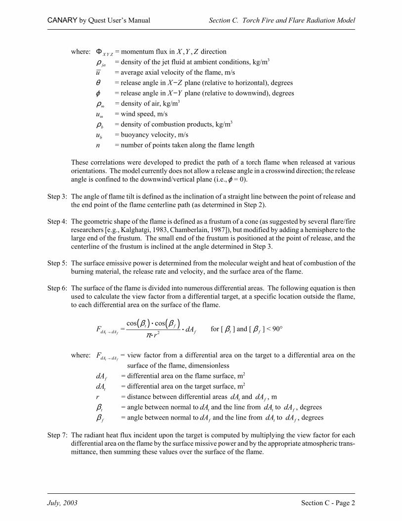
where: = momentum flux in directionX Y ZΦ , ,X Y Z = density of the jet fluid at ambient conditions, kg/m3

jaρ = average axial velocity of the flame, m/su = release angle in plane (relative to horizontal), degreesθ X Z− = release angle in plane (relative to downwind), degreesϕ X Y−

= density of air, kg/m3ρ∞

= wind speed, m/su∞

= density of combustion products, kg/m3bρ = buoyancy velocity, m/sbu

= number of points taken along the flame lengthn

These correlations were developed to predict the path of a torch flame when released at variousorientations. The model currently does not allow a release angle in a crosswind direction; the releaseangle is confined to the downwind/vertical plane (i.e., = 0).ϕ

Step 3: The angle of flame tilt is defined as the inclination of a straight line between the point of release andthe end point of the flame centerline path (as determined in Step 2).

Step 4: The geometric shape of the flame is defined as a frustum of a cone (as suggested by several flare/fireresearchers [e.g., Kalghatgi, 1983, Chamberlain, 1987]), but modified by adding a hemisphere to thelarge end of the frustum. The small end of the frustum is positioned at the point of release, and thecenterline of the frustum is inclined at the angle determined in Step 3.

Step 5: The surface emissive power is determined from the molecular weight and heat of combustion of theburning material, the release rate and velocity, and the surface area of the flame.

Step 6: The surface of the flame is divided into numerous differential areas. The following equation is thenused to calculate the view factor from a differential target, at a specific location outside the flame,to each differential area on the surface of the flame.

= for [ ] and [ ] < 90°t fdA dAF →

( ) ( )2

cos cost ffdA

rβ β

πi

ii

tβ fβ

where: = view factor from a differential area on the target to a differential area on thet fdA dAF →

surface of the flame, dimensionless= differential area on the flame surface, m2

fdA= differential area on the target surface, m2

tdA= distance between differential areas and mr tdA ,fdA= angle between normal to and the line from to degreestβ tdA tdA ,fdA= angle between normal to and the line from to degreesfβ fdA tdA ,fdA

Step 7: The radiant heat flux incident upon the target is computed by multiplying the view factor for eachdifferential area on the flame by the surface missive power and by the appropriate atmospheric trans-mittance, then summing these values over the surface of the flame.



=a iqt f

f

sf dA dAA

q F τ→∑ i i

where: = attenuated radiant heat flux incident upon the target due to radiant heat emitted by thea iqflame, kW/m2

= area of the surface of the flamefA= radiant heat flux emitted by the surface of the flame, kW/m2

s fq= atmospheric transmittance, dimensionlessτ

Atmospheric transmittance, is a function of absolute humidity and the path length between,τ ,rdifferential areas on the flame and target [Wayne, 1991].

Step 8: Steps 6 and 7 are repeated for numerous target locations.

Validation

Several of the equations used in the Torch Fire and Flare Radiation Model are empirical relationships basedon data from medium- to large-scale experiments, which ensures reasonably good agreement between modelpredictions and experimental data for variables such as flame tilt angle. Comparisons of experimental dataand model predictions for incident heat flux at specific locations are more meaningful and of greater interest.Unfortunately, few reports on medium- or large-scale experiments contain the level of detail required to makesuch comparisons.

One reasonable source of test data is a report by Chamberlain [1987]. It contains data from seven flare testsinvolving natural gas releases from industrial flares, with several data points being reported for each test.Variables that were examined during these tests include release diameter (0.203 and 1.07 m), release rate andvelocity, and wind speed. Figure C-1 compares the predicted values of incident heat flux with experimentaldata from the seven flare tests.

References

Chamberlain, G. A., “Developments in Design Methods for Predicting Thermal Radiation from Flares.”Chemical Engineering Research and Design, Vol. 65, July, 1987.

Cook, D. K., M. Fairweather, G. Hankinson, and K. O’Brien, “Flaring of Natural Gas from Inclined VentStacks.” IChemE Symposium Series #102, Pergamon Press, 1987.

Kalghatgi, G. T., “The Visible Shape and Size of a Turbulent Hydrocarbon Jet Diffusion Flame in a CrossWind.” Combustion and Flame, Vol. 52, 1983: pp. 91-106.




0 2 4 6 8 10

Flare Test Data, kW/m2

0

2

4

6

8

10

CA

NA

RY

Pre

dict

ions

, kW

/m2

Test Series 3Test Series 4

Figure C-1

CANARY by Quest User’s Manual Section D. Fireball Model

July, 2003 Section D - Page 1

Fireball Model

Purpose

The purpose of the Fireball Model is to predict the impact of thermal radiation emitted by fireballs that resultfrom catastrophic failures of pressure vessels containing superheated liquids. Specifically, the model predictsthe average radiant heat flux incident upon a grade-level target as a function of the horizontal distancebetween the target and the center of the fireball.

Required Data

(a) Composition of flammable liquid within the pressure vessel(b) Mass of flammable liquid within the pressure vessel(c) Pressure within vessel just prior to rupture(d) Temperature of the liquid within the vessel just prior to rupture(e) Air temperature(f) Relative humidity

Methodology

Step 1: Calculate the mass of fuel consumed in the fireball. The mass of fuel in the fireball is equal to thesmaller of the mass of fuel in the vessel (as specified by the user), or three times the mass of fuel thatflashes to vapor when it is released to the atmosphere [Hasegawa and Sato, 1977].

Step 2: Calculate the maximum diameter of the fireball using the empirical correlation from Roberts[1981/82].

= maxD 1/ 35.8 fMi

where: = maximum diameter of the fireball, mmaxD = mass of fuel in the fireball, kgfM

Step 3: Calculate fireball duration using the following empirical correlation [Martinsen and Marx, 1999].

= dt1/ 40.9 fMi

where: = fireball duration, sdt= mass of fuel in the fireball, kgfM

Step 4: Calculate the size of the fireball and its location, as a function of time. The fireball is assumed togrow at a rate that is proportional to the cube root of time, reaching its maximum diameter, ,maxDat the time of liftoff, During its growth phase, the fireball remains tangent to grade. After/ 3.dtliftoff, it rises at a constant rate [Shield, 1994].



Step 5: Estimate the surface flux of the fireball. The fraction of the total available heat energy that is emittedas radiation is calculated using the equation derived by Roberts [1981/82].

=f 0.320.0296 Pi

where: = fraction of available heat energy released as radiation, dimensionlessf= pressure in vessel at time of rupture, kPaP

The total amount of energy emitted as radiation is then calculated.

= rE f cf M H∆i i

where: = energy emitted as radiation, kJrE= heat of combustion, kJ/kgcH∆

The surface flux is estimated by dividing by the average surface area of the fireball and the fireballrEduration, but it is not allowed to exceed 400 kW/m2.

Step 6: Calculate the maximum view factor from a differential target (at specific grade level locations outsidethe fireball) to the fireball, using the simple equation for a spherical radiator [Howell, 1982].

=F2

2

RH

where: = view factor from differential area to the fireball, dimensionlessF = radius of the fireball, mR= distance between target and the center of the fireball, mH

and vary with time due to the growth and rise of the fireball. Therefore, the duration of theR Hfireball is divided into time intervals and a view factor is calculated at the end of each interval.

Step 7: Compute the attenuated radiant heat flux at each target location, at the end of each time interval,by multiplying the appropriate view factor by the surface flux of the fireball and by the appropriateatmospheric transmittance. The transmittance of the atmosphere is a function of the absolute humid-ity and path length from the fireball to the target [Wayne, 1991]. For each target location, calculatethe average attenuated heat flux over the duration of the fireball.

Step 8: Calculate the absorbed energy at each target location. For a given location, the energy absorbedduring each time interval is computed by multiplying the length of the interval by the averageattenuated radiant heat flux for that interval. The absorbed energies for all time intervals are thensummed to determine the radiant energy absorbed over the duration of the fireball.

Step 9: Calculate the integrated dosage at each target location. This is computed in the same manner asabsorbed energy is computed in Step 8, except that the average attenuated radiant heat flux for eachtime interval is taken to the 4/3rds power before it is multiplied by the time interval. This allows thedosage to be used in the probit equation for fatalities from thermal radiation [Eisenberg, Lynch, andBreeding, 1975].



Figure D-1

= Pr ( )4 / 338.4785 2.56 ln q t− + i i

where: = probitPr= radiant heat flux, W/m2q= exposure time, st

Validation

Several of the equations used in the Fireball Model are empirical relationships based on data from small- tomedium-scale experiments, which ensures reasonably good agreement between model predictions andexperimental data for variables such as maximum fireball diameter. Comparisons of experimental data andmodel predictions for average incident heat flux, absorbed energy, or dosage are more meaningful and ofgreater interest. Unfortunately, very few reports on small- or medium-scale fireball experiments contain thelevel of detail required to make such comparisons, and no such data are available for large-scale experiments.

One of the most complete sources of test data for medium-scale fireball tests is a report by Johnson, Pritchard,and Wickens [1990]. It contains data on five BLEVE tests that involved butane and propane, in quantitiesup to 2,000 kg. Figure D-1 compares the predicted values of absorbed energy with experimental data fromthose five BLEVE tests.



References

Eisenberg, N. A., C. J. Lynch, and R. J. Breeding, Vulnerability Model: A Simulation System for AssessingDamage Resulting from Marine Spills. U.S. Coast Guard, Report CG-D-136-75, June, 1975.

Hasegawa, K., and K. Sato, “Study on the Fireball Following Steam Explosion of n-Pentane.” Proceedingsof the Second International Symposium on Loss Prevention and Safety Promotion in the Process Indus-tries, Heidelberg, Germany, September, 1977: pp. 297-304.

Howell, John R., A Catalog of Radiation Configuration Factors. McGraw-Hill Book Company, 1982.

Johnson, D. M., M. J. Pritchard, and M. J. Wickens, Large-Scale Catastrophic Releases of FlammableLiquids. Commission of European Communities, Report EV4T.0014, 1990.

Martinsen, W. E., and J. D. Marx, “An Improved Model for the Prediction of Radiant Heat from Fireballs.”Presented at the 1999 International Conference and Workshop on Modeling Consequences of AccidentalReleases of Hazardous Materials, San Francisco, California, September 28 - October 1, 1999.

Roberts, A. F., “Thermal Radiation Hazards from Releases of LPG from Pressurized Storage.” Fire SafetyJournal, Vol. 4, 1981/82: pp. 197-212.

Shield, S. R., Consequence Modeling for LPG Distribution in Hong Kong. Thornton Research Centre, Safetyand Environment Department, United Kingdom, TNRN 95.7001, December 13, 1994.


CANARY by Quest User’s Manual Section E. Fluid Release Model

July, 2003 Section E - Page 1

Fluid Release Model

Purpose

The purpose of the Fluid Release Model is to predict the rate of mass release from a breach of containment.Specifically, the model predicts the rate of flow and the physical state (liquid, two-phase, or gas) of therelease of a fluid stream as it enters the atmosphere from a circular breach in a pipe or vessel wall. The modelalso computes the amount of vapor and aerosol produced and the rate at which liquid reaches the ground.

Required Data

(a) Composition of the fluid(b) Temperature and pressure of the fluid just prior to the time of the breach(c) Normal flow rate of fluid into the vessel or in the pipe(d) Size of the pipe and/or vessel(e) Length of pipe(f) Area of the breach(g) Angle of release relative to horizontal(h) Elevation of release point above grade

Methodology

Step 1: Calculation of Initial Flow Conditions

The initial conditions (before the breach occurs) in the piping and/or vessel are determined from theinput data, coupled with a calculation to determine the initial pressure profile in the piping. Thepressure profile is computed by dividing the pipe into small incremental lengths and computing theflow conditions stepwise from the vessel to the breach point. As the flow conditions are computed,the time required for a sonic wave to traverse each section is also computed. The flow in any lengthincrement can be all vapor, all liquid, or two-phase (this implies that the sonic velocity within eachsection may vary). As flow conditions are computed in each length increment, checks are made todetermine if the fluid velocity has exceeded the sonic velocity or if the pressure in the flow incrementhas reached atmospheric. If either condition has been reached, an error code is generated andcomputations are stopped.

Step 2: Initial Unsteady State Flow Calculations

When a breach occurs in a system with piping, a disturbance in flow and pressure propagates fromthe breach point at the local sonic velocity of the fluid. During the time required for the disturbanceto reach the upstream end of the piping, a period of highly unsteady flow occurs. The portion of thepiping that has experienced the passage of the pressure disturbance is in accelerated flow, while theportion upstream of the disturbance is in the same flow regime as before the breach occurred.

To compute the flow rate from the breach during the initial unsteady flow period, a small timeincrement is selected and the distance that the pressure disturbance has moved in that time incrementis computed using the sonic velocity profile found in the initial pressure profile calculation. The



disturbed length is subdivided into small increments for use in an iterative pressure balancecalculation. A pressure balance is achieved when a breach pressure is found that balances the flowfrom the breach and the flow in the disturbed section of piping. Another time increment is added,and the iterative procedure continues. The unsteady period continues until the pressure disturbancereaches the upstream end of the pipe.

Step 3: Long-Term Unsteady State Flow Calculations

The long-term unsteady state flow calculations are characterized by flow in the piping system thatis changing more slowly than during the initial unsteady state calculations. The length of acceleratedflow in the piping is constant, set by the user input pipe length. The vessel contents are being deplet-ed, resulting in a potential lowering of pressure in the vessel. As with the other flow calculations,the time is incremented and the vessel conditions are computed. The new vessel conditions serve asinput for the pressure drop calculations in the pipe. When a breach pressure is computed thatbalances the breach flow with the flow in the piping, a solution for that time is achieved. The solu-tion continues until the ending time or other ending conditions are reached.

The frictional losses in the piping system are computed using the equation:

= (1)h24

2ls

c e

f L Ug D

i i i

i i

where: = head (pressure) loss, ft of fluidh = friction factorf = length of system, ftL = average flowing velocity, ft/secU= gravitational constant, 32.2 lbm • ft/(lbf • sec2)cg= equivalent diameter of duct, fteD

The friction factor is computed using the following equation:

= (2)1f

102 18.71.74 2.0 log

eD Re fε − +

ii

i

where: = pipe roughness, ftε= Reynolds number, , dimensionlessRe /eD U ρ µi i

= fluid density, lb/ft3ρ= fluid viscosity, lb/(ft • sec)µ

Equations (1) and (2) are used for liquid, vapor, and two-phase flow regimes. Since the piping issubdivided into small lengths, changes in velocity and physical properties across each segment areassumed to be negligible. At each step in the calculation, a check is made to determine if the fluidvelocity has reached or exceeded the computed critical (sonic) velocity for the fluid. If the criticalvelocity has been exceeded, the velocity is constrained to the critical velocity and the maximum massflow rate in the piping has been set.



If the fluid in the piping is in two-phase flow, the Lockhart and Martinelli [1949] modification toEquation (1) is used. The Lockhart and Martinelli equation for head loss is shown below:

= (3)TPh2

2 42

ls

c e

f L Ug D

Φ

i i ii

i i

where: = head loss for two-phase flow, ft of fluidTPh= empirical parameter correlating single- and two-phase flow, dimensionlessΦ= superficial liquid velocity (velocity of liquid if liquid filled the pipe), ft/seclsU

This equation is valid over short distances where the flowing velocity does not change appreciably.

Validation

Validation of fluid flow models is difficult since little data are available for comparison. Fletcher [1983]presented a set of data for flashing CFC-11 flowing through orifices and piping. Figures E-1 through E-4compare calculations made using the Fluid Release Model with the data presented by Fletcher. Figure E-1compares fluid fluxes for orifice type releases. These releases had length-to-diameter (L/D) ratios less than0.88. Figure E-2 compares computed and experimental release fluxes for an L/D ratio of 120 at several levelsof storage pressure. Figure E-3 compares similar releases for an L/D of 37.5. Figure E-4 shows predictedand experimental release fluxes at a given pressure for L/D ratios from 1 to 200.

Figures E-5 and E-6 compare computed and experimental gas discharge rates for the complete breach of twopipes. One pipe had an internal diameter of 6.2 inches (0.157 m); the other had a diameter of 12 inches (0.305m). These pipes were initially pressurized to 1,000 psia with air and then explosively ruptured. Theexperimental values were reported in a research paper for Alberta Environment, authored by Wilson [1981].

Aerosols and Liquid Droplet Evaporation

Liquids stored at temperatures above their atmospheric pressure boiling point (superheated liquids) will giveoff vapor when released from storage. If the temperature of storage is sufficiently above the normal boilingpoint, the energy of the released vapor will break the liquid stream into small droplets. If these droplets aresmall enough, they will not settle, but remain in the vapor stream as aerosol droplets. The presence of aerosoldroplets in the vapor stream changes its apparent density and provides an additional source of vapor. Dropletslarge enough to fall to the ground will lose mass due to evaporation during their fall.

The prediction of aerosol formation and amount of aerosol formed is based on the theoretical work performedfor the Center for Chemical Process Safety (CCPS) by CREARE. CREARE’s work has been extended andcorrected by Quest. The extension to the model computes the non-aerosol drop evaporation. In Figure E-7,the four experimental data sets available for comparison (chlorine (Cl2), methylamine (MMA), CFC-11, andcyclohexane) are compared to the values computed by the CANARY Aerosol Model.



0 1 2 3 4 5System Pressure, barg

0

5000

10000

15000

20000

Mas

s Fl

ux, k

g/(m

2 -s)

ExperimentalComputed

Figure E-1Comparison of CFC-11 Orifice Releases as a Function of System Pressure

0 1 2 3 4System Pressure, barg

0

1000

2000

3000

4000

5000

6000

7000

Mas

s Fl

ux, k

g/(m

2 -s)


Figure E-2CFC-11 Release Rate Comparison with L/D of 120



0 1 2 3 4System Pressure, barg

0

1000

2000

3000

4000

5000

6000

7000

Mas

s Fl

ux, k

g/(m

2 -s)


Figure E-3CFC-11 Release Rate Comparison with L/D of 37.5

0 20 40 60 80 100 120 140 160 180 200

Length/Diameter Ratio

0

4000

8000

12000

16000

Mas

s Fl

ux, k

g/(m

2 -s)


Figure E-4CFC-11 Release Rate Comparison at Varying L/D Ratios



0 10 20 30 40 50 60 70Time, sec

10

100

2

3

4

5

6

789

2

3

4

Mas

s R

ate,

kg/

sec


Figure E-5Air Discharge Rates for 0.157 m Diameter Piping

0 20 40 60 80 100Time, sec

100

1000

8

9

2

3

4

5

6

7

8

9

Mas

s R

ate,

kg/

sec


Figure E-6Air Discharge Rates for 0.305 m Diameter Piping



230 250 270 290 310 330 350 370 390 410

Temperature, K

0

10

20

30

40

50

60

70

80

90

100

110

Perc

ent o

f Liq

uid

to G

roun

d (N

orm

aliz

ed to

100

% a

t NB

P)

Cl2 MMA CFC-11 Cyclohexane

Figure E-7Aerosol Formation as a Function of Storage Temperature

References

Fletcher, B., “Flashing Flow Through Orifices and Pipes.” Paper presented at the AIChE Loss PreventionSymposium, Denver, Colorado, 1983.

Lockhart, R. W., and R. C. Martinelli, “Proposed Correlation of Data for Isothermal Two-Phase, Two-Component Flow in Pipes.” Chemical Engineering Progress, Vol. 45, 1949: p. 39.

Wilson, D. J., “Expansion and Plume Rise of Gas Jets from High Pressure Pipeline Ruptures.” ResearchPaper, Pollution Control Division, Alberta Environment, April, 1981.

CANARY by Quest User’s Manual Section F. Momentum Jet Dispersion Model

July, 2003 Section F - Page 1

Momentum Jet Dispersion Model

Purpose

The purpose of this model is to predict the dispersion of a jet release into ambient air. It is used to predictthe downwind travel of a flammable or toxic gas or aerosol momentum jet release.

Required Data

(a) Composition and properties of the released material(b) Temperature of released material(c) Release rate of material(d) Vertical release angle relative to wind direction(e) Height of release(f) Release area(g) Ambient wind speed(h) Ambient Pasquill-Gifford stability class(i) Ambient temperature(j) Relative humidity(k) Surface roughness scale

Methodology

Step 1: An assumption is made that flow perpendicular to the main flow in the plume is negligible, that thevelocity and concentration profiles in the jet are similar at all sections of the jet, that molecular trans-port in the jet is negligible, and that longitudinal turbulent transport is negligible when compared tolongitudinal convective transport. The coordinate system is then defined in and where is thes ,r spath length of the plume and is the radial distance from the plume centerline. The angle betweenrthe plume axis and horizontal is referred to as Relationships between the downwind coordinate, .θ ,xvertical coordinate, and plume axis are given simply by:,y

= (1)dxds

( )cos θ

and

= (2)d yd s

( )sin θ

Step 2: Velocity, concentration, and density profiles are assumed to be cylindrically symmetric about theplume axis and are assumed to be Gaussian in shape. The three profiles are taken as:

= (3)( ), ,u s r θ ( ) ( ) ( )

2

2*cosr

b saU u s eθ

−

+i i



where: = plume velocity, m/su= ambient wind speed, m/saU= plume velocity relative to the wind in the downwind direction at the plume axis, m/s*u= characteristic width of the plume at distance from the release, m( )b s s

= (4)( ), ,s rρ θ ( ) ( )

2

2 2*rb s

a s e λρ ρ−

+ ii

where: = plume density, kg/m3ρ = density of ambient air, kg/m3 aρ

= density difference between plume axis and ambient air, kg/m3( )* sρ = turbulent Schmidt number, 1.352λ

= (5)( ), ,c s r θ ( ) ( )

2

2 2*r

b sc s e λ−ii

where: = pollutant concentration in the plume, kg/m3c= pollutant concentration at plume centerline, kg/m3( )*c s

Step 3: The equation for air entrainment into the plume and the conservation equations can then be solved.The equation for air entrainment is:

(6)( )2

02bd u dr

dsρ π∫ i i i i

= ( ) ( ) ( ){ }*1 2 32 sin cosa ab u s U uπ ρ α α θ θ α ′+ +i i i i i i i i

where: = entrainment coefficient for a free jet, 0.0571α = entrainment coefficient for a line thermal, 0.52α = entrainment coefficient due to turbulence, 1.03α = turbulent entrainment velocity (root mean square of the wind velocity fluctuation isu′ used for this number), m/s

Step 4: The equations of conservation of mass, momentum, and energy are given as:

= 0 (7)( )2

02bd c u dr

dsπ∫ i i i i

(8)( )( )( )2 2

0cos 2bd u dr

dsρ θ π∫ i i i i i

= ( ) ( ) ( ){ }*1 2 32 sin cosa ab u s U uπ ρ α α θ θ α ′+ +i i i i i i i i i

+ ( )2 sind a aC b Uπ ρ θi i i i



(9)( )( )2 2

0cos 2

bd u drds

ρ θ π∫ i i i i i

= ( ) ( ) ( )2 2

0sin cos

b

a d a ag r dr C b Uρ ρ π π ρ θ θ− ±∫ i i i i i i i i i

(10)2

00

1 1 2b

a

d u r drd s

ρ πρ ρ

−

∫ i i i i i

= ( ) ( ) ( ){ }*1 2 3

0

1 12 | | sin | cosa aa a

b u s U úρ π α α θ θ αρ ρ

− + +

i i i i i i i i

The subscript refers to conditions at the point of release. These equations are integrated along the0path of the plume to yield the concentration profiles as a function of elevation and distance down-wind of the release.

Step 5: After the steady-state equations are solved, an along-wind dispersion correction is applied to accountfor short-duration releases. This is accomplished using the method outlined by Palazzi, et al. [1982].

Step 6: If the plume reaches the ground, it is coupled to the Heavy Gas Dispersion Model (described inSection G) and the dispersion calculations continue.

Validation

The Momentum Jet Dispersion Model used in CANARY was validated by comparing results obtained fromthe model with experimental data from field tests. Data used for this comparison and the conditions used inthe model were taken from an American Petroleum Institute (API) study [Hanna, Strimaitis, and Chang,1991]. For this model, comparisons were made with the Desert Tortoise, Goldfish, and Prairie Grass seriesof dispersion tests. Results of these comparisons are shown in Figure F-1.

References

Astleford, W. J., T. B. Morrow, and J. C. Buckingham, Hazardous Chemical Vapor Handbook for MarineTank Vessels (Final Report – Phase II). U.S. Coast Guard Report No. CG-D-12-83, April, 1983.

Hanna, S. R., D. G. Strimaitis, and J. C. Chang, Hazard Response Modeling Uncertainty (A QuantitativeMethod), Evaluation of Commonly Used Hazardous Gas Dispersion Models, Volume II. Study co-sponsored by the Air Force Engineering and Services Center, Tyndall Air Force Base, Florida, and theAmerican Petroleum Institute; performed by Sigma Research Corporation, Westford, Massachusetts,September, 1991.

Havens, J., and T. Spicer, LNG Vapor Dispersion Prediction with the DEGADIS Dense Gas DispersionModel. Gas Research Institute Contract No. 5086-252-1287 with the University of Arkansas, September,1990: pp. 37-48.

Ooms, G., “A New Method for the Calculation of the Plume Path of Gases Emitted by a Stack.” AtmosphericEnvironment, Vol. 6, 1972: pp. 889-909.



10-2 10-1 100 101 102 103 104 105 10610-2

10-1

100

101

102

103

104

105

106

Desert Tortoise (NH3)Goldfish (HF)Prarie Grass (SO2)

OVERPREDICTION

UNDERPREDICTION

Flammable RangeTrace Gas Range

Field Data Concentration (ppm)

CAN

ARY

Pre

dict

ed C

once

ntra

tion

(ppm

)

Figure F-1

Ooms, G., A. P. Mahieu, and F. Zelis, “The Plume Path of Vent Gases Heavier than Air.” First InternationalSymposium on Loss Prevention and Safety Promotion in the Process Industries, C. H. Buschman, Editor,Elsevier Press, 1974.

Palazzi, E., M. De Faveri, G. Fumarola, and G. Ferraiolo, “Diffusion from a Steady Source of Short Dura-tion.” Atmospheric Environment, Vol. 16, No. 12, 1982: pp. 2785-2790.

CANARY by Quest User’s Manual Section G. Heavy Gas Dispersion Model

July, 2003 Section G - Page 1

Heavy Gas Dispersion Model

Purpose

The purpose of this model is to predict the dispersion and gravity flow of a heavy gas released into the airfrom liquid pools or instantaneous gas releases. It is used to predict the downwind travel of a flammable ortoxic vapor cloud.

Required Data

(a) Composition and properties of the released material(b) Temperature of released material(c) Vapor generation rate(d) Vapor source area(e) Vapor source duration(f) Ambient wind speed(g) Ambient Pasquill-Gifford atmospheric stability class(h) Ambient temperature(i) Relative humidity(j) Surface roughness scale

Methodology

Step 1: For a steady-state plume, released from a stationary source, the Heavy Gas Dispersion Model solvesthe following equations:

= (1)( )d U B h mdx

ρ i i i i s s sW Bρ i i

= (2)( )d U B hdx

ρ i i i ( )a e e s s sV h W B W Bρ ρ+ +i i i i i

= (3)( )pd U B h C Tdx

ρ i i i i i ( )a e e pa a s s s ps s tV h W B C T W B C T fρ ρ+ + +i i i i i i i i i

( )d U B h Udx

ρ i i i i

=

(4)

( ) ( )20.5 g a a e e a udg B h V h W B U fdx

α ρ ρ ρ − − + + + i i i i i i i i i

= (5)( )gd U B h Vdx

ρ i i i i ( ) 2a vgg h fρ ρ− +i i



= (6)cdZUdx

i cg

ZVB

− i

= (7)dBUdxi a

e gV Vρρ

+i

= (8)Tρ i( )a a s

s a s

T MM M M m

ρ+ −

i i

i

where: = downwind distance, mx= density, kg/m3ρ= velocity in the direction of the wind, m/sU= cloud width parameter, mB= cloud height parameter, mh= mass fraction of source gasm= temperature, KT= specific heat, J/(kg K)pC i

= ground heat flux, J/(m s)tf i

= downwind friction term, kg/s2uf

= crosswind friction term, kg/s2vf

= horizontal entrainment rate, m/seV= horizontal crosswind gravity flow velocity, m/sgV= vertical entrainment rate, m/seW= vertical source gas injection velocity, m/ssW= molecular weight, kg/kmoleM= refers to source propertiess= refers to ambient propertiesa

The first six equations are crosswind-averaged conservation equations. Equation (7) is the widthequation, and Equation (8) is the equation of state.

Step 2: All of the gas cloud properties are crosswind averaged. The three-dimensional concentration distri-bution is calculated from the average mass concentration by assuming the following concentrationprofile:

= (9)( ), ,C x y z ( ) ( ) ( )1 2C x C y C zi i

= (10)( )C x( )

( ) ( )a

s a s

M m xM M M m x+ −

i

i

= (11)( )1C y 14 2 2

y b y berf erfb β β

+ − − i

i i i



= (12)2B 2 23b β+ i

= (13)( )2C z1/ 2 2

2

6 1 3exp2

zh hπ

−

ii i

i

where: = concentration in plume at kg/m3( ), ,C x y z , , ,x y z= crosswind coordinate, my= vertical coordinate, mz= half-width parameters, m, ,b B β

Step 3: As there are now two parameters used to define the following equation is needed to calcu-( )1 ,C ylate :b

= (14)dbUdx

i g

bVB

i

Step 4: The vertical entrainment rate is defined to be:

= (15)eW3

h

ha k UH

hL

δ∗

Φ

i i i i

where: = constant, 1.5a= constant, 0.41k= friction velocity, m/sU ∗

= Monin-Obukhov length derived from the atmospheric stability classL

Step 5: The profile function is used to account for the height of the mixing layer, and to restrict theδ ,Hgrowth of the cloud height to that of the mixing layer. is a function of stability class and is defin-Hed as:

= (16)hH

δ

1 hH

−

The Monin-Obukhov function, is defined by:,hΦ

= (17)hhL

Φ 1/ 2

1 5 0 (stable)

1 16 0 (unstable)

h LL

h LL

−

+ ≥

− <

i

i

Step 6: After the steady-state equations are solved, an along-wind dispersion correction is applied to accountfor short-duration releases. This is accomplished using the method outlined by Palazzi, et al. [1982].



10-2 10-1 100 101 102 103 104 105 10610-2

10-1

100

101

102

103

104

105

106

Burro (LNG)Coyote (LNG)Maplin Sands (LNG & LPG)

OVERPREDICTION

UNDERPREDICTION

Flammable RangeTrace Gas Range

Field Data Concentration (ppm)

CAN

ARY

Pred

icte

d C

once

ntra

tion

(ppm

)

Figure G-1

Validation

The Heavy Gas Dispersion Model used in CANARY was validated by comparing results obtained from themodel with experimental data from field tests. Data used for this comparison and the conditions used in themodel were taken from an American Petroleum Institute (API) study [Hanna, Strimaitis, and Chang, 1991].For this model, comparisons were made with the Burro, Maplin Sands, and Coyote series of dispersion tests.Results of these comparisons are shown in Figure G-1.

References

Ermak, D. L., and S. T. Chan, A Study of Heavy Gas Effects on the Atmospheric Dispersion of Dense Gases.UCRL-92494, Lawrence Livermore National Laboratory, Livermore, California. Presented at the 15thNATO/CCMS International Technical Meeting on Air Pollution Modeling and Its Applications, St.Louis, Missouri, April 15-19, 1985.

Ermak, D. L., S. T. Chan, D. L. Morgan, Jr., and L. K. Morris, “A Comparison of Dense Gas DispersionModel Simulations with Burro Series LNG Spill Test Results.” Journal of Hazardous Materials, Vol.6, 1982: pp. 129-160.

Ermak, D. L., and S. T. Chan, Recent Developments on the FEM3 and SLAB Atmospheric Dispersion Models.UCRL-94071, Lawrence Livermore National Laboratory, Livermore, California. Presented at the IMAConference on Stably Stratified Flows and Dense Gas Dispersion, Chester, England, April 9-10, 1986.

Hanna, S. R., D. G. Strimaitis, and J. C. Chang, Hazard Response Modeling Uncertainty (A QuantitativeMethod), Evaluation of Commonly-Used Hazardous Gas Dispersion Models, Volume II. Studycosponsored by the Air Force Engineering and Services Center, Tyndall Air Force Base, Florida, and the



American Petroleum Institute; performed by Sigma Research Corporation, Westford, Massachusetts,September, 1991.

Morgan, D. L., L. K. Morris, S. T. Chan, D. L. Ermak, T. G. McRae, R. T. Cederwall, R. P. Kooperman, H.C. Goldwire, Jr., J. W. McClure, and W. J. Hogan, Phenomenology and Modeling of Liquefied NaturalGas Vapor Dispersion. UCRL-53581, Lawrence Livermore National Laboratory, Livermore, California,1982.

Morgan, D. L., Jr., L. K. Morris, and D. L. Ermak, SLAB: A Time-Dependent Computer Model for theDispersion of Heavy Gases Released in the Atmosphere. UCRL-53383, Lawrence Livermore NationalLaboratory, Livermore, California, 1983.

Palazzi, E., M. De Faveri, G. Fumarola, and G. Ferraiolo, “Diffusion from a Steady Source of Short Dura-tion.” Atmospheric Environment, Vol. 16, No. 12, 1982: pp. 2785-2790.

CANARY by Quest User’s Manual Section I. Vapor Cloud Explosion Model

July, 2003 Section I - Page 1

Vapor Cloud Explosion Model

Purpose

The purpose of this model is to predict the overpressure field that would be produced by the explosion of apartially confined and/or obstructed fuel-air cloud, based on the Baker-Strehlow methodology. Specifically,the model predicts the magnitude of the peak side-on overpressure and specific impulse as a function ofdistance from the source of the explosion.

Required Data

(a) Composition of the fuel (flammable fluid) involved in the explosion(b) Total mass of fuel in the flammable cloud at the time of ignition or the volume of the partially-confined/

obstructed area(c) Fuel reactivity (high, medium, or low)(d) Obstacle density (high, medium, or low)(e) Flame expansion (1-D, 2-D, 2½-D, or 3-D)(f) Reflection factor

Methodology

Step 1: The combustion energy of the cloud is estimated by multiplying its mass by the heat of combustion.If the volume of the flammable cloud is input, the mass is estimated by assuming that a stoichiometricmixture of gas and air exists within that volume.

Step 2: The combustion energy is multiplied by the reflection factor to account for blast reflection from theground or surrounding objects.

Step 3: Flame speed is determined from the fuel reactivity, obstacle density, and flame expansion parameters,as presented in Baker, et al. [1994, 1998].

Fuel reactivity and obstacle density each have low, medium, and high choices. The flame expansionparameter allows choices of 1-D, 2-D, 2.5-D, and 3-D. The choices for these three parameters createa matrix of 36 possibilities, thus allowing locations that have differing levels of congestion or con-finement to produce different overpressures. Each matrix possibility corresponds to a flame speed,and thus a peak (source) overpressure. The meanings of the three parameters and their options are:

Fuel Reactivity (High, Medium, or Low). The fuels considered to have high reactivity areacetylene, ethylene oxide, propylene oxide, and hydrogen. Low reactivity fuels are (pure)methane and carbon monoxide. All other fuels are medium reactivity. If fuels from differentreactivity categories are mixed, the model recommends using the higher category unless theamount of higher reactivity fuel is less than 2% of the mixture.

Obstacle Density (High, Medium, or Low). High obstacle density is encountered whenobjects in the flame’s path are closely spaced. This is defined as multiple layers of obstruc-tion resulting in at least a 40% blockage ratio (i.e., 40% of the volume is occupied by

CANARY by Quest User’s Manual Section I. Vapor Cloud Explosion Model

July, 2003 Section I - Page 2

obstacles). Low density areas are defined as having a blockage ratio of less than 10%. Allother blockage ratios fall into the medium category.

Flame Expansion (1-D, 2-D, 2.5-D, or 3-D). The expansion of the flame front must be char-acterized with one of these four descriptors. 1-D expansion is likened to an explosion in apipe or hallway. 2-D expansion can be described as what occurs between flat, parallel sur-faces. An unconfined (hemispherical expansion) case is described as 3-D. The additionaldescriptor of 2.5-D is used for situations that begin as 2-D and quickly transition to 3-D.

Step 4: Based on the calculated flame speed, appropriate blast curves are selected from the figures in Baker,et al., 1994. For flame speeds not shown on the graph, appropriate curves are prepared by interpola-tion between existing curves.

Step 5: The Sachs scaled distance, is calculated for several distances using the equation:,R

= R 1/ 3

0

R

EP

where: = distance from the center of the explosionR= total energy calculated in step 2, aboveE= atmospheric pressure0P

Step 6: The peak side-on overpressure and specific impulse at each scaled distance are determined from theblast curves in Baker, et al., 1994.

References

Baker, Q. A., M. J. Tang, E. Scheier, and G. J. Silva, “Vapor Cloud Explosion Analysis.” 28th Loss Preven-tion Symposium, AIChE, 1994.

Baker, Q. A., C. M. Doolittle, G. A. Fitzgerald, and M. J. Tang, “Recent Developments in the Baker-StrehlowVCE Analysis Methodology.” Process Safety Progress, 1998: p. 297.

Date post:	18-Apr-2018
Category:	Documents
Upload:	nguyenthuan
View:	216 times
Download:	1 times

WORST-CASE CONSEQUENCE ANALYSIS FOR...

Documents