X-Ray Diffraction

Eric ReichweinBryce Burgess

Department of PhysicsUniversity of California, Santa Cruz

February 3, 2014

1

Contents

1 Introduction 31.1 Historical Background . . . . . . . . . . . . . . . . . . . . . . . . . . . . . . 31.2 Physics of X-Ray Diffraction . . . . . . . . . . . . . . . . . . . . . . . . . . . 4

2 Experimental Setup and Procedure 52.1 Preparing Samples . . . . . . . . . . . . . . . . . . . . . . . . . . . . . . . . 52.2 Diffractometer . . . . . . . . . . . . . . . . . . . . . . . . . . . . . . . . . . . 5

3 Data and Analysis 63.1 Aluminum and Vaseline Holder . . . . . . . . . . . . . . . . . . . . . . . . . 63.2 Silicon Crystals . . . . . . . . . . . . . . . . . . . . . . . . . . . . . . . . . . 83.3 Table Salt (NaCl) . . . . . . . . . . . . . . . . . . . . . . . . . . . . . . . . . 103.4 Cobalt (II, III) Oxide Co3O4 . . . . . . . . . . . . . . . . . . . . . . . . . . . 113.5 Unknown . . . . . . . . . . . . . . . . . . . . . . . . . . . . . . . . . . . . . 14

4 Conclusion 15

2

1 Introduction

This laboratory studies the atomic crystalline structure of 5 compounds, including one un-known compound which we are to determine. Using powder X-Ray Diffraction (XRD) andpowerful refinement software called FullProf we discovered the inner structure of these com-pounds. We used two XRD machines courtesy of the chemistry department.

1.1 Historical Background

It is often thought the pioneers of XRD were father and son team of Sir William HenryBragg and William Lawrence Bragg. However, they merely showed that diffraction can bethought of as reflection between two crystal planes and then used it to determine the crystalstructure of numerous compounds. When in fact the first discovery of XRD was done byMax von Laue and his colleagues Paul Knipping and Walter Friedrich in 1912. [4] Laue firsthypothesized, after learning that X-rays had wavelengths corresponding on the atomic scale,that X-rays would be diffracted when passing through substances. [3] In Fig. 1 you can seethe first ever diffraction pattern done by von Laue. The Bragg’s saw von Laue’s work andbuilt upon it and refined it the following year in 1913. The Bragg’s subsequently won theNobel Prize in physics for their work on XRD in 1915.

Figure 1: Max von Laue and the first ever XRD pattern (copper sulfate).

Over the following years the equipment improved and the analysis was enhanced, but themajor contribution for this laboratory was made by Hugo Rietveld in the 1960’s. He usednon-linear least squares approach to fit the experimental data. This allows for finer precisionin determining the properties of the crystals we are studying. The FullProf software doesthe Rietveld refinement for us, so we will neglect the theory of it, for sake of clarity.

With out a doubt XRD has been extremely useful in all areas of science, not just physics.For instance, the structure of DNA was discovered by James Watson and Francis Crick in1954 using the XRD data that Rosalind Franklin had produced, see Fig. 2 for the diffractionpattern of DNA. XRD was the first and is still one of the most efficient and accurate way

3

to probe the atomic scales. In total there has been 14 Nobel Prizes awarded for study ofX-Rays and X-Ray diffraction.[2]

Figure 2: Rosalind Franklin and the XRD pattern of DNA.

1.2 Physics of X-Ray Diffraction

As mentioned previously he Bragg’s showed that diffraction is geometrically equivalent toreflection of off parallel lattice planes.

Figure 3: Bragg’s Law [?]

As seen in Fig.3 the X-Rays come in parallel and leave parallel. One X-ray reflects offof the lattice plane below the surface lattice plane. Since the lower X-Ray travels a fartherdistance it will be out of phase with the upper X-Ray. X-Rays being electromagnetic waveshowever, will have points are constructive (meaning the phase is an even integer times π)or destructive (meaning the phase is an odd integer times π) . In terms of wavelengths theconstructive condition is that the extra distance the lower X-Ray must travel are integerwavelengths. The extra distance can be found geometrically using Fig. 3. Going into thesample the lower X-Ray still has the distance dsinθ to go until it is reflected. After it isreflected the lower X-Ray has another d sin θ to go until it’s direction is perpendicular to theupper X-Rays direction at the location of the uppers reflection point. This essentially means

4

that there are certain angles at which you will get constructive interference, since ideally, dis constant. This can be mathematically expressed by Eq. 1

nλ = 2d sin θ (1)

Where n is any integer, λ is the wavelength of the X-Rays, d is the atomic latticeplane spacing, and θ is the angle of entry. This equation can be interpreted as (numberof wavelengths)=(total extra distance traveled by lower X-Ray).

2 Experimental Setup and Procedure

2.1 Preparing Samples

To use the X-Ray machine for powder diffraction we lathered Vaseline onto the slides thenplaced the powder onto the slides. The Vaseline is to prevent the powder from falling offof the slides because the sample mount rotated as well as the detector. Due to the largegrain size of the table salt and the unknown compound we had to grind the samples untilit was a fine powder. The other compounds were already fine enough for accurate readings.We measured the diffraction pattern from a sample holder with Vaseline to compare to oursamples to differentiate true signal from background signal.

2.2 Diffractometer

A diffractometer is essentially and X-Ray source and a X-Ray detector on a movable arm.Most commonly the X-Ray source is stationary and the sample mount and X-Ray detectorare movable. See Fig. 4 below for a diagram of Diffractometer.

Figure 4: Diagram of diffractometer.

We used two different types of diffractometers (both manufactured by Rigaku) becausecobalt oxide fluoresces. The first diffractometer did not have a monochromator in between thesample and the detector. The monochromator blocks all electromagnetic radiation outside

5

of a given bandwidth. The location of the monochromator is key because if we placed itbetween the source and the sample then the X-Rays caused by fluorescence of the samplewould still be created and picked up by the detector. The difference in intensities can be seenin the cobalt oxide data. For the data without the monochromator we see a large increasein intensity as a function of θ. This for obvious reasons makes it difficult to fit the data tostandard purely diffracted peaks. Refer to reference [1] for more details on the diffractometeras well as our lab report on X-Ray fluorescence.

3 Data and Analysis

Our raw data comes in the form of data files which can be either plotted as 2θ vs. intensity(I) or opened using FullProf and analyzed through the program. Through FullProf wealso produced visualizations of the crystal lattices. For the following graphs the red linecorresponds to the actual data, the black thin line corresponds to the fit function, the blueline is the difference between the fit and the data and the green dashes represent knownlattice planes. Note that the relative intensities change between the graphs correspondingto different number of lattice planes, preferred orientations, uniformity of crystal powder.

Our refinement algorithm for all samples is as follows:

1. Vary background polynomial, B factor and intensity scale . Fix all other parameters.Repeat this until fit function peak positions match data.

2. Let a, b, c vary with previous variable parameters fixed.

3. Fix a, b, c values. Then vary (until convergence) u, v, w one at a time.

4. Refine B factor again with new u, v and w values.

This allowed for the most accurate fitting of data. Following this algorithm gives usconsistency between fits as well.

3.1 Aluminum and Vaseline Holder

The first peak we analyzed was the sample holder so we distinguish background from actualsignal. We use aluminum sample holders because it has very distinct, sharp peaks thatare easily subtracted from other data. The grayed out region of the data is due to theVaseline. We will see a slight bump for the other samples at 2θ angles of less than 25◦.Every other peak is characteristic of aluminum as marked by the green dashes. From theICSD database (reference [5]) we found that the space group for aluminum was F m -3 m.Using the .cif file (crystallographic information file) from the ICSD database we inputtedthe lattice parameters and ran Rietveld refinement of the fit function.

6

Figure 5: Aluminum sample holder with Vaseline. The gray region corresponds to theVaseline so we excluded it for fitting the aluminum data.

Note that the fit function peaks are slightly off actual data peaks. This is becauseirregularities in the samples crystals. This is most notably seen at the 2θ = 78.5◦ peakand is indicative of the preferred orientation. Also, note that the double peak at an angle2θ = 43.5◦. We believe this is also attributed to the irregularities in the sample such asdefects and impurities.

Figure 6: Aluminum crystal structure. It is a face centered cubic with space group F m -3m.

7

Since aluminum is face centered cubic (FCC) then we know that α = β = γ = 90◦ andthat a = b = c = 4.05 A. We summarize our results below.

Table 1: Crystallographic planes and lattice spacing of aluminum.

Peak (2θ) (hkl) dhkl

38.5◦ (111) 2.34A43.5◦ (200) 2.03A65.0◦ (220) 1.43A72.0◦ (311) 1.22A82.5◦ (222) 1.17A

The last column dhkl is the lattice spacing d in Eq. 1. We calculate dhkl by the followingformula

1

dhkl=

√h2

a2+k2

b2+l2

c2(2)

Where h, k, l are the Miller indices and a, b, c are the lattice parameters.

3.2 Silicon Crystals

Silicon is a FCC just like aluminum, however, it has a basis as well that gives it a diamondstructure. The space group is F m -3 m: 1. The extra : 1 accounts for the basis vectors. Thestructure factor comes into play for silicon because we have peak cancellation. The structurefactor F tells you how the X-Rays interact with atoms, the f is characteristic of each typeof atom. The larger the F the larger the intensity (I ∝ |F |2 ). The structure rules of silicon(and all diamond shaped crystals) are:

• h, k, l have mixed parity then F 2 = 0

• h, k, l are all odd then F 2 = 32f 2

• h, k, l are all even and exactly divisible by 4 then F = 8f

• h, k, l are all even and not divisible by 4 then F 2 = 0

This tells us that there are two groups of crystal planes that give us peak cancellationand two groups that don’t. We see in Fig. 7 that there is only peak that is canceled in ourdata corresponding to a 2θ = 58.5◦. There is also extra peaks corresponding to the samepeaks that we saw in the aluminum sample holder. Those peaks are 2θ = 38.5◦, 43.5◦, 65.0◦

and 82.5◦ which all correspond to the peaks of aluminum.

8

Figure 7: Diffraction pattern of silicon crystals

The lattice vectors are a = b = c = 5.43Aand the vector angles are α = β = γ = 90.0◦

since silicon is FCC. In Table 2, we can see that the structure factor rules are followed.There are no mixed parity Miller indices and the (222) plane adds up to 6 which is notexactly divisible by four. Notice in Fig. 7 that there are two peaks for the (311) plane whichindicates that there is a dislocation defect in line with this plane. The preferred orientationappears to be (111), but with (220) closely behind it. The difference in intensities of thesetwo peaks is approximately 75.

Table 2: Crystallographic planes and lattice spacing of silicon.

Peak (2θ) (hkl) dhkl Canceled

28.5◦ (111) 3.13A No47.5◦ (220) 1.92A No56.0◦ (311) 1.63A No59.0◦ (222) 1.57A Yes69.0◦ (400) 1.36A No76.5◦ (331) 1.25A No

Comparing our a value to established a values of 5.431Awe see that there is very littledifference to the number of significant digits. One thing to note here is that even thoughwe have four extra basis vectors, we only get one extra lattice plane. This is due to thesymmetry of the diamond structure. We show below the atomic structure of the siliconcrystals from two different perspectives. The green, red and blue axis correspond to the a, band c directions, respectively. However, due to the cubic structure and symmetry of thediamond these are arbitrary and could be switched in any combination without harm.

9

Figure 8: Silicon FCC crystallographic structure. We show two different perspectives of thediamond structure due to its complexity of having four extra basis atoms.

3.3 Table Salt (NaCl)

Sodium chloride is a very common compound with crystalline structure. The average saltcrystal is much too large to get accurate data so we first ground the salt to a very finepowder.

Figure 9: Diffraction pattern of salt crystals.

At first glance of Fig. 9 you may think there are two canceled peaks, however, lookingmore closely (and looking at difference line) we see that they are actually a near perfect fit.There are no extra peaks so we know all peaks correspond to NaCl. The space group of saltis F m -3 m. Once again we have α = β = γ = 90◦ which corresponds to cubic structure,more specifically a body centered cubic (BCC). The lattice vectors are a = b = c = 5.66Aandhave a basis (corresponding to the Cl− atoms). In Table 3 we summarize the data of thenine peaks.

10

Table 3: Crystallographic planes and lattice spacing of table salt.

Peak (2θ) (hkl) dhkl

27.0◦ (111) 3.27A31.5◦ (200) 2.83A45.5◦ (220) 1.99A54.0◦ (311) 1.71A56.0◦ (222) 1.63A66.0◦ (400) 1.41A73.0◦ (331) 1.30A75.0◦ (222) 1.27A

It is clear from the peak shapes that there is a preferred orientation of (200). The smallpeaks are due to the structure factor rules of NaCl, but we have predicted the intensitiesquite well using FullProf and Rietveld refinement. As you can see in Fig. 10, it is easierto see NaCl’s atomic structure because of the chlorine basis, as compared to the diamondstructure of silicon.

Figure 10: NaCl crystallographic structure. Smaller atoms correspond to the sodium (Na+)and larger correspond to the chlorine (Cl−).

3.4 Cobalt (II, III) Oxide Co3O4

Cobalt oxide is an antiferromagnet and extremely harmful compound for the environment.Below in Fig. 11 we show a comparison between NaCl (red) and Co3O4 (thick dark blue).As you can see its diffraction pattern is very unique. This is because we are actually seeingX-Ray fluorescence of the compound. To learn more about X-Ray fluorescence see our first

11

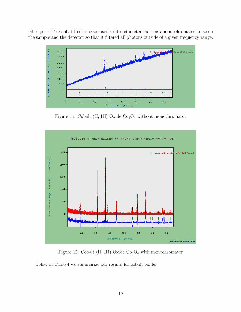
lab report. To combat this issue we used a diffractometer that has a monochromator betweenthe sample and the detector so that it filtered all photons outside of a given frequency range.

Figure 11: Cobalt (II, III) Oxide Co3O4 without monochromator

Figure 12: Cobalt (II, III) Oxide Co3O4 with monochromator

Below in Table 4 we summarize our results for cobalt oxide.

12

Table 4: Crystallographic planes and lattice spacing of table salt.

Peak (2θ) (hkl) dhkl

19.0◦ (111) 4.66A31.0◦ (220) 2.85A37.0◦ (311) 2.43A38.5◦ (222) 2.33A45.0◦ (400) 2.02A49.0◦ (331) 1.85A56.0◦ (422) 1.65A59.5◦ (333) 1.55A59.5◦ (511) 1.55A65.0◦ (440) 1.42A68.5◦ (531) 1.36A70.0◦ (442) 1.34A74.0◦ (620) 1.27A77.5◦ (533) 1.23A78.5◦ (622) 1.21A83.0◦ (444) 1.17A

In Fig. 13 below we present the atomic structure of the cobalt oxide. The lattice param-eters are α = β = γ = 90◦ and a = b = c = 8.07A.

Figure 13: Cobalt (II, III) Oxide Co3O4 atomic structure.

13

3.5 Unknown

For our unknown sample we tried using the .cif files from each compound we had. We foundthat the NaCl .cif file corresponded the best to the unknown data. Seeing the similarities incrystal structure, space group, and looks to NaCl we decided that it was KCl, another formof table salt.

Figure 14: Unknown

Notice that all peaks are accounted for except the 2θ = 75◦. This assumed to be dueto defects or irregularities for that particular lattice plane. Just as we did for all the otherelements we present the results summarized in Table 5 below.

14

Table 5: Crystallographic planes and lattice spacing of table salt.

Peak (2θ) (hkl) dhkl

27.0◦ (111) 3.27A31.5◦ (200) 2.83A45.5◦ (220) 2.00A54.0◦ (311) 1.71A56.0◦ (222) 1.63A66.0◦ (400) 1.41A73.0◦ (331) 1.30A75.0◦ (222) 1.27A75.0◦ (422) 1.15A

Comparing Table 5 to Table 3 we see that there is a very close correspondence, supportingour claim that the unknown sample is indeed KCl. The first peak is barely noticeable asmentioned in the lab manual as well. The lattice parameters are α = β = γ = 90◦ anda = b = c = 5.66A.

4 Conclusion

We have conducted X-Ray diffraction experiments on 4 known samples and one unknownsample. Using powerful software (FullProf) we were able to get the most accurate fits of thediffraction data. This gave us the ability to calculate numerous aspects of atomic structures ofcrystalline structures. Using FullProf we were also able to extract beautiful crystal structureimages from data. We notice that with increasing angle we got a smaller dhkl, which is whatwe would expect for this data.

We wish we had more time to do a more careful and in depth analysis of each of thediffraction patterns. However, from just aligning peak positions we believe that it wassufficient to get the necessary data.

Some improvements we would suggest is to shorten the lab manual. Just present theactual lab and analysis methods, and let the student to do research onto the nitty grittydetails. I believe FullProf should be a requirement as well. It is very powerful and essentiallyall scientists doing diffraction experiments. The FullProf manual could be accompanied bysome screen shots for clarity, but overall it was very well written and explained.

References

[1] Durand, Alice. Physics 134 Lab Manual XRD. Winter 2014.

[2] Willmot, Phillip. Introduction to Synchrotron Radiation and its Applications. 2011.Wiley.

[3] http://epswww.unm.edu/xrd/xrdclass/03-GenX-rays.pdf

15

[4] http://www.chemistryviews.org/details/ezine

[5] FIZ Karlsruhe ICSD. 2012. https://icsd.fiz-karlsruhe.de/. Accessed 3/2014.

16