X-Ray Fluorescence Analytical

Techniques

Moussa Bounakhla

& Mounia Tahri

CNESTEN

CONTENT

SECTION I: Basic in X-Ray Fluorescence

I. History of X-Ray Fluorescence

II. Introduction

III. Physics of X-Rays

III.1 Electromagnetic Radiation, Quanta

III.2 Properties of X-Rays

III.3 The Origin of X-Rays

III.4 Bohr’s Atomic Model

III.5 Nomenclature

III.6 X-Ray Emission

III.6.1 Continuum

III.6.2 Characteristic Emission

III.7 Interactions of X-Ray with Matter

III.7.1 Photoelectric Absorption

III.7.2 Compton Effect

III.7.3 Rayleigh Scattering (Elastic Scattering)

III.7.4 Competitive Interactions

III.8 Fluorescence Yield

IV. X-Ray Production Sources

IV.1 X-Ray Tubes

IV.1.1 Side-window Tubes

IV.1.2 End-window Tubes

IV.2 Radioisotope Sources

SECTION II: Energy Dispersive X-Ray Fluorescence (ED-XRF)

I. Introduction

II. Instrumentation

II.1 Excitation Mode

II.1.1 Direct Tube Excitation

II.1.2 Secondary Target Excitation

II.1.3 Radio-Isotopic Excitation

II.2 Detectors

II.3 Pulse Height Analysis

II.4 Energy Resolution

III. Spectrum Evaluation

IV. Detector Artefacts

IV.1 Escape Peaks

IV.2 Compton Edge

IV.3 Resulting Spectral Background

V. The Approach to Quantification in EDXRF Analysis

V.1 Thin Samples Technique

V.2 Intermediate Thickness Samples

V.3 Infinitely Thick Samples

SECTION III: Total Reflexion X-Ray Fluorescence (TXRF)

I. Introduction

II. Advantages of TXRF

III. Principle of Total Reflection X-Ray Fluorescence Analysis

IV. Instrumentation

IV.1 Excitation Sources for TXRF

IV.2 Sample Reflectors

IV.3 Detectors

V. Quantification

VI. Influence on Detection Limits

VII. General Sample Preparation

VIII. Application of TXRF

SECTION IV: Wavelength Dispersive X-Ray Fluorescence (WD-XRF)

I. Introduction

II. Principle of WD-XRF

II.1 Collimator Masks

II.2 Collimator

II.3 Analyzing Crystals

II.3.1 Bragg’s Law

II.3.2 Reflections of Higher Orders

II.3.3 Crystal Types

II.3.4 Dispersion, Line Separation

II.3.5 Synthetic Multilayers

II.4 Detectors

II.4.1 Gas Proportional Counter

II.4.2 Scintillation Counters

II.4.3 Pulse Height Analysis (PHA), Pulse Height Distribution

III. Points of Comparison between ED-XRF and WD-XRF

SECTION V: Sample Preparation

I. Solids

II. Powders and Briquets

III. Fused Materials

IV. Filters and Ions-Exchange Resins

V. Thin Films

VI. Liquids

SECTION VI: Quantitative Analysis

I. Detection Limits

II. Disturbing Effects

II.1 Interelement Radiation

II.2 Matrix Effects

II.2.1 Absorption Effect

II.2.2 Enhancement Effect

II.3 Particle-Size Effects

II.4 Mineralogical Effects

II.5 Surface Effects

III. Mathematical Models

III.1 Sherman Equation

III.2 Empirical Alpha Models

III.3 Fundamental Parameters Method

III.4 Fundamental Alphas

III.5 Semi-Quantitative Analysis

Exercises and Solutions

Module: Title: X-Ray Fluorescence Analytical Techniques

Learning objective:

Make potential users proficient in the use of X-Ray Fluorescence Analytical Techniques Target public:

Potential users including students in science and technology Profile:

Senior technicians, Students, Teachers, Researchers and Analytical Specialists in Scientific Fields. Qualifications:

University education related to application of sciences and technology English and French literacy

SECTION I

BASIC IN X-RAY FLUORESCENCE I. History of X-Ray Fluorescence

The history of X-ray fluorescence dates back to the accidental discovery of X-rays in 1895 by the German physicist Wilhelm Conrad Roentgen. While studying cathode rays in a high-voltage, gaseous-discharge tube, Roentgen observed that even though the experimental tube was encased in a black cardboard box the barium-platinocyanide screen, which was lying adjacent to the experiment, emitted fluorescent light whenever the tube was in operation. Roentgen's discovery of X-rays and their possible use in analytical chemistry went unnoticed until 1913. In 1913, H.G.J. Mosley showed the relationship between atomic number (Z) and the reciprocal of the wavelength (1/λ) for each spectral series of emission lines for each element. Today this relationship is expressed as:

2)sZ(a/c −=λ ; (I.1)

where: a is a proportionality constant, s is a constant dependent on a periodic series.

Mosley was also responsible for the construction of the early X-ray spectrometer. His design centered around a cold cathode tube where the air within the tube provided the electrons and the analyte which served as the tube target. The major problem experienced laid in the inefficiency of using electrons to create x-rays; nearly 99% of the energy was lost as heat.

In the same year, the Bragg brothers built their first X-ray analytical device. Their device was based around a pinhole and slit collimator. Like Mosley's instrument, the Braggs ran into difficulty in maintaining efficiency. Progress in XRF spectroscopy continued in 1922 when Hadding investigated using XRF spectrometry to analyse mineral samples. Three years later, Coster and Nishina put forward the idea of replacing electrons with X-ray photons to excite secondary X-ray radiation resulting in the generation of an X-ray spectrum. This technique was attempted by Glocker and Schrieber, who in 1928 published Quantitative Roentgen Spectrum Analysis by Means of Cold Excitation of the Spectrum in Ann. Physics.

Progress appeared to be at a standstill until 1948, when Friedman and Birks built the first XRF spectrometer. Their device was built around a diffractometer, with a Geiger counter for a detection device and proved comparatively sensitive for much of the atomic number range. It might be noted that XRF spectrometers have progressed to the point where elements ranging from Beryllium to Uranium can be analysed.

Although the earliest commercial XRF devices used simple air path conditions, machines were soon developed utilizing helium or vacuum paths, permitting the detection of lighter elements. In the 1960’s, XRF devices began to use lithium fluoride crystals for diffraction and chromium or rhodium target X-ray tubes to excite longer wavelengths. This development was quickly followed by that of multichannel spectrometers for the simultaneous measurement of many elements. By the mid 60’s computer controlled XRF devices were coming into use. In 1970, the lithium drifted silicon detector (Si(Li)) was created, providing

very high resolution and X-ray photon separation without the use of an analysing crystal. An XRF device was even included on the Apollo 15 and 16 missions.

Meanwhile, Schwenke and co-workers have fine tuned a procedure known as total reflection X-ray fluorescence (TXRF), which is now used extensively for trace analysis. In TXRF, a Si(Li) detector is positioned almost on top of a thin film of sample, many times positioned on a quarts plate. The primary radiation enters the sample at an angle that is only slightly smaller than the critical angle for reflection. This significantly lowers the background scattering and fluorescence, permitting the detection of concentrations of only a few tenths of a ppb.

II. Introduction

X-ray Fluorescence (XRF) Spectroscopy involves measuring the intensity of X-rays emitted from a specimen as a function of energy or wavelength. The energies of large intensity lines are characteristic of atoms of the specimen. The intensities of observed lines for a given atom vary as the amount of that atom present in the specimen. Qualitative analysis involves identifying atoms present in a specimen by associating observed characteristic lines with their atoms. Quantitative analysis involves determining the amount of each atom present in the specimen from the intensity of measured characteristic X-ray lines.

The emission of characteristic atomic X-ray photons occurs when a vacancy in an inner electron state is formed, and an outer orbit electron makes a transition to that vacant state. The energy of the emitted photon is equal to the difference in electron energy levels of the transition. As the electron energy levels are characteristic of the atom, the energy of the emitted photon is characteristic of the atom. Molecular bonds generally occur between outer electrons of a molecule leaving inner electron states unperturbed. As X-ray fluorescence involves transitions to inner electron states, the energy of characteristic X-ray radiation is usually unaffected by molecular chemistry. This makes XRF a powerful tool of chemical analysis in all kinds of materials.

In a liquid, fluoresced X-rays are usually little affected by other atoms in the liquid and line intensities are usually directly proportional to the amount of that atom present in the liquid. In a solid, atoms of the specimen both absorb and enhance characteristic X-ray radiation. These interactions are termed 'matrix effects' and much of quantitative analysis with XRF spectroscopy is concerned with correcting for these effects.

While the principles are the same, a variety of instrumentation is used for performing X-ray fluorescence spectroscopy. There are two basic classes of instruments: Wavelength Dispersive and Energy Dispersive. Wavelength Dispersive spectrometers measure X-ray intensity as a function of Wavelength while Energy Dispersive spectrometers measure X-ray intensity as a function of energy.

An extremely important aspect of X-ray fluorescence spectroscopy is the method by which the inner orbital vacancy is created. Bombarding the sample with high energy X-rays is one method. Bombarding with high-energy electrons and protons are other approaches. An incident photon beam experiences a photon absorption interaction with the specimen while electron and proton beams primarily experience a Coulomb interaction with the specimen.

X-ray tubes accelerate high-energy electrons at a target within the tube that is then caused to fluoresce X-rays. The resulting X-ray beam includes a continuum and characteristic lines of the tube target. Radioactive sources can also be used to generate X-ray, electron (beta

emitters), and proton (alpha emitters) beams. X-ray tubes can generate a high power X-ray beam, but the radiation is not monochromatic. Radioactive sources produce monochromatic beams, but of comparatively lower power. Proton-Induced X-ray Emission (PIXE) utilises a beam of protons. Wavelength Dispersive Spectrometry (WDS) generally utilises an X-ray tube as does Energy Dispersive X-ray Spectrometry (EDX). Instruments such as the electron microprobe and electron microscope directly bombard the sample with high-energy electrons to eject inner orbital electrons (EDS). Note that the charged particle beam approaches require the specimen to be electrically conductive.

III. Physics of X-Rays

III.1 Electromagnetic Radiation, Quanta

X rays are electromagnetic radiation. All X-rays represent a very energetic portion of the electromagnetic spectrum (Table 1) and have short wavelengths of about 0.1 to 100 angstroms (Å). They are bounded by ultraviolet light at long wavelengths and gamma rays at short wavelengths X-rays in the range from 50 to 100 Å are termed soft X-rays because they have lower energies and are easily absorbed.

Table I.1: Energy and names of various wavelength range.

Energy range (eV) Wavelength range Name

< 10-7 cm to km Radio Waves (short, medium, long waves)< 10-3 mm to cm Micro Wave < 10-3 mm to mm Infra Red 0.0017 – 0.0033 380 to 750 nm Visible Light 0.033 – 0.1 10 to 380 nm Ultra Violet 0.11 - 100 0.01 to 12 nm X-Rays 10 - 5000 0.0002 to 0.12 nm Gamma Radiation

The range of interest for X-ray is approximately from 0.1 to 100 Å. Although, angstroms are used throughout these notes, they are not accepted as SI unit. Wavelengths should be expressed in nanometers (nm), which are 10-9 meters (1 Å = 10-10 m), but most texts and articles on microprobe analysis retain the use of the angstroms. Another commonly used unit is the micron, which more correctly should be termed micrometer (µm); a micrometer is 104 Å.

The relationship between the wavelength of electromagnetic radiation and its corpuscular energy (E) is derived as follows. For all electromagnetic radiation:

ν= hE ; (I.2)

where:

h is the Planck constant (6.62 10-24 J.s);

ν is the frequency expressed in Hertz.

For all wavelengths,

λ=ν /c ; (I.3)

where: c = speed of light (2.99782 108 m/s); λ= wavelength (Å).

Thus:

λ=λ= − /1098636.1/hcE 24 ; (I.4)

where E is in Joule and λ in meters.

The conversion to angstroms and electron volts (1 eV = 1.6021 10-19 Joule) yields the Duane-Hunt equation:

)A(/396.12)eV(Eo

λ= . (I.5)

Note the inversion relationship. Short wavelengths correspond to high energies and long wavelengths to low energies. Energies for the range of X-ray wavelengths are 124 keV (0.1 Å) to 124 eV (100 Å). The magnitudes of X-ray energies suggested to early workers that X-rays are produced from within an atom. Those produced from a material consist of two distinct superimposed components: continuum (or white) radiation, which has a continuous distribution of intensities over all wavelengths, and characteristic radiation, which occurs as a peak of variable intensity at discrete wavelengths.

III.2 Properties of X-Rays

A general summary of the properties of X-rays is presented below:

• Invisible; • Propagate with velocity of light (3.108 m/s) • Unaffected by electrical and magnetic fields; • Differentially absorbed in passing through matter of varying composition, density and

thickness; • Reflected, diffracted, refracted and polarized; • Capable of ionising gases; • Capable of affecting electrical properties of solids and liquids; • Capable of blackening a photographic plate; • Able to liberate photoelectron. And recoils electrons • Emitted in a continuous spectrum; • Emitted also with a line spectrum characteristic of the chemical element; • Found to have absorption spectra characteristic of the chemical element.

III.3 The Origin of X-Rays

An electron can be ejected from its atomic orbital by the absorption of a light wave (photon) of sufficient energy. The energy of the photon (hν) must be greater than the energy with which the electron is bound to the nucleus of the atom. When an inner orbital electron is ejected from an atom, an electron from a higher energy level orbital will transfer into the vacant lower energy orbital (Figure I.1). During this transition a photon may be emitted from the atom. To understand the processes in the atomic shell, we must take a look at the Bohr’s atomic model.

The energy of the emitted photon will be equal to the difference in energies between the two orbitals occupied by the electron making the transition. Due to the fact that the energy difference between two specific orbital shells, in a given element, is always the same (i.e., characteristic of a particular element), the photon emitted when an electron moves between these two levels will always have the same energy. Therefore, by determining the energy (wavelength) of the X-ray light (photons) emitted by a particular element, it is possible to determine the identity of that element.

Figure I.1: A pictorial representation of X-ray fluorescence using a generic atom and

generic energy levels. This picture uses the Bohr model of atomic structure and is not to scale.

III.4 Bohr’s Atomic Model

Bohr’s atomic model describes the structure of an atom as an atomic nucleus surrounded by electron shells (Figure I.2). The positively charged nucleus is surrounded by electrons that move within defined areas (shell). The differences in the strength of the electron’s bonds to the atomic nucleus are very clear depending on the area or level they occupy, i.e., they vary in their energy. When we talk about this, we refer to energy levels or energy shells. This means that a clearly defined minimum amount of energy is required to release an electron of the innermost shell from the atom. To release an electron of the second innermost shell from the atom, a clearly defined minimum amount of energy is required that is lower that that needed to release an innermost electron. An electron’s bond to an atom is weaker the further away it is from the atom’s nucleus. The minimum amount of energy required .to release an electron from an atom, and thus the energy with which it is bound to the atom, is also referred to as the binding energy of the electron to the atom.

Figure I.2: Bohr’s atomic model, shell model.

The binding energy of an electron in an atom is established mainly by determining the incident. It is for this reason that the term absorption edge is very often found in literature.

Energy level = binding energy = absorption edge The individual shells are labelled with the letters K, L; M; N, …, the innermost shell

being the K-shell, the second innermost the L-shell etc. the K-shell is occupied by 2 electrons; the L-shell has three sub-levels and can contain up to a total of 8 electrons. The M-shell has five sub-levels and can contain up to 18 electrons.

III.5 Nomenclature

The production of X-rays involves transitions of the orbital electrons at atoms in the target between allowed orbits or energy states, associated with ionization of the inner atomic shell. The permissible transitions that electrons can undergo from initial to final state are specified by three quantum selection rules: 1. The change in n must be ≥ 1 (∆n ≠ 1); 2. The change in l only can be ±1; 3. The change in j can only be ±1 or 0.

When an electron is ejected from the K-shell by electron bombardment or by the absorption of a photon, the atom becomes ionized. If this electron vacancy is filled by an electron coming from an L shell, the transition is accompanied by the emission of an X-ray line known as K line; this process leaves a vacancy in the L shell. On the other hand, the vacancy in the L shell might be filled by an electron coming from the M shell that is accompanied by the emission of an L line (Figure I.3). The terminology of energy levels and X-ray lines are showed in Figure I.4.

Figure I.3: Schematic illustration of production of K and L lines.

Figure I.4: X-ray line labelling.

III.6 X-Ray Emission

X-rays re generated from the disturbance of the electron orbitals of atoms. This may be accomplished in several ways, the most common of which is to bombard a target element with high energy electrons, X-rays or accelerated charged particles. The first two are frequently used in X-ray spectrometry, either directly or indirectly. Electron bombardment results in both a continuum of X-ray energies and radiation that is characteristic of the target elements. Because both types of radiation will be encountered in X-ray spectrometry, each will be discussed.

III.6.1 Continuum

Continuum X-rays are produced when electrons or high energy charged particles lose energy in passing through the Coulomb field of a nucleus. In this interaction, the radiant energy (photon) lost by the electron is called Bremsstrahlung (Figure I.5). The emission of continuous X-rays finds a simple explanation in terms of classic electromagnetic theory, since according to this; the acceleration of charged particles should be accompanied by emission of radiation. In the case of high energy electrons striking a target, they must be rapidly

decelerated as they penetrate the material of target, and such a high negative acceleration should produce a pulse of radiation.

Figure I.5: On the left, the classical model showing the production of Bremsstrahlung.On the right, the Continuum X-ray emission spectrum.

The probability of radiative energy loss (Bremsstrahlung) is roughly proportional to q2z2T/M0

2, where q is the particle charge in units of the electron charge e, Z is the atomic number of the target material, T is the particle kinetic energy, and M0 is the rest mass of the particle. Because of the fact that protons and heavier particles have large masses, compared to the electron mass, they irradiate relatively little, e.g., the intensity of continuous X-rays generated by protons is about four orders of magnitude lower than the generated by electrons.

The ratio of energy lost by Bremsstrahlung to that lost by ionization can be approximated by:

20

2

0

0

cm1600TZ

Mm

⎟⎟⎠

⎞⎜⎜⎝

⎛, (I.6)

where m0 is the rest of the electron.

III.6.2 Characteristic Emission

The purpose of X-ray fluorescence is to determine chemical elements both qualitatively and quantitatively by measuring their characteristic radiation. To do this, the chemical elements in a sample must be caused emit X-rays. As characteristic X-rays only rise in the transition of atomic shell electron to lower, vacant energy levels of the atom, a method must be applied that is suitable for releasing electrons from the innermost shell of an atom. This involves adding to the inner electrons amounts of energy that are higher than the energy bonding them to the atom.

This can be done in a number ways:

• Irradiation using elementary particles of sufficient energy (electrons, protons, a-particles…) that transfer the energy necessary for release to the atomic shell electrons during collision processes.

• Irradiation using X- or gamma rays from radionuclides. • Irradiation using X-rays from an X-ray tube.

III.7 X-Ray Interactions with Matter

When X-rays are directed into an object, some of the photons interact with the particles of the matter and their energy can be absorbed or scattered. This absorption and scattering is called attenuation. Other photons travel completely through the object without interacting with any of the materials particles. The number of photons transmitted through a material depends on the thickness, density and atomic number of the material, and the energy of the individual photons.

Even when they have the same energy, photons travel different distances within a material simply based on the probability of their encounter with one or more of the particles of the matter and the type of encounter that occur. Since the probability of an encounter increases with the distances travelled, the umber of photons reaching a specific point within the matter decreases exponentially with distance travelled (Figure I.6).

Figure I.6: Exponential attenuation of photon energy with distance travelled in the

material. The formula that describes this curve is:

x0 eII µ−= (Beer-Lambert law); (I.7)

where: I0 is the initial intensity of photons; µ is the linear absorption coefficient; X is the distance travelled.

The linear absorption coefficient has the dimension [1/cm] and is depend on the energy

or the wavelength of the X-ray quants and the special density ρ (in [g/cm3]) of the material that was passed through.

It is not the linear absorption coefficient that is specific to the absorptive properties of the element, but the coefficient applicable to the density ρ of the material that was passed through:

µ/ρ = mass attenuation coefficient.

The mass attenuation coefficient has the dimension [cm2/g] and only depends on the atomic number of the absorber element and the energy, or wavelength, of the X-ray quants.

The mass attenuation coefficient accounts for the various interactions and is therefore composed of here major components:

)E()E()E()E( inccoh σ+σ+τ=µ ; (I.8)

τ(E) is the photoelectric mass absorption coefficient; σcoh(E) is the coherent mass absorption coefficient; σinc(E) is the incoherent mass absorption coefficient.

III.7.1 Photoelectric Absorption

In the photoelectric interaction, a photon transfers all its energy to an electron located in one of the atomic shells (Figure I.7). The electron is ejected from the atom by this energy and begins to pass through the surrounding matter. The electron rapidly loses its energy and moves only a relatively short distance from its original location. The photon’s energy is, therefore, deposited in the matter close to the site of the photoelectric interaction. The energy transfer is a two-step process. The photoelectric interaction in which the photon transfers its energy to the electron is the first step. The depositing of the energy in the surrounding matter by the electron is the second step.

Photoelectric interactions usually occur with electrons that are firmly bound to the atom, that is, those with a relatively high binding energy. Photoelectric interactions are most probable when the electron binding energy is only slightly less than the energy of the photon. If the binding energy is more than the energy of the photon, a photoelectric interaction cannot occur. This interaction is possible only when the photon has sufficient energy to overcome the binding energy and remove the electron from the atom. The probability of photoelectric interactions occurring is also dependent on the atomic number of the material. An explanation for the increase, the binding energies move closer to the photon energy. The general relationship is that the probability of photoelectric interactions is proportional to Z3. In general, the conditions that increase the probability of photoelectric interactions are low photon energies and high atomic number materials.

This process is often the major contributor of the absorption X-rays, and is the mode of excitation of the X-rays spectra emitted by elements in samples. Primarily as a result of the photoelectric process, the mass absorption coefficient decreases steadily with increasing energy of the incident X-radiation. There are sharp discontinuities at which the photoelectric process is especially efficient. Energies at which these discontinuities occur are called absorption edges (Figure I.8).

Figure I.7: Schematic description of photoelectric principle.

Figure I.8: Absorption edges for different shells.

The Figure I.8 supplies the following:

• The overall progression of the coefficient decreases as energy increases, i.e. the higher the energy of the X-ray quants, the less they are absorbed.

• The rapid changes in the mass attenuation coefficient reveal the binding energies of the electrons in the appropriate shells. If an X-ray quant has a level of energy that is equivalent to the binding energy of an atomic shell electron in an appropriate shell, it is then able to transfer all its energy to this electron and displace it from the atom. In this case, absorption increases sharply. Quants whose energy is only slightly below the absorption edge are absorbed far less rapidly.

III.7.2 Compton Effect

Also known as incoherent scattering, Compton effect is the interaction of a photon with a free electron that is considered to be at the rest. The weak binding of electrons to atoms may

be neglected provided that momentum transferred to the electron greatly exceeds the momentum of the electron in the bound state. Figure I.9 shows the Compton effect schematically.

Relativistic energy and momentum are conserved in this process and the scattered X-ray photon has less energy and therefore a longer wavelength than the incident photon. Compton scattering is important for low atomic number specimens.

The change in wavelength of the scattered photon is given by:

)cos1(cm

hcc

oo

oθ−=λ−λ′=

ν−

ν′. (I.9)

Theta is the scattering angle of the scattered photon.

Figure I.9: Compton effect.

III.7.3 Rayleigh Scattering (Elastic Scattering)

Elastic scattering is a process by which photons are scattered by bound atomic electrons and in which the atom is neither ionized nor excited. The incident photons are scattered with unchanged energy and with a definite phase relation between incoming and scattered waves (Figure I.10). The intensity of the radiation scattered by an atom is determined by summing the amplitudes of the radiation coherently scattered by each of the electrons bound in the atom. It should be emphasized that coherence extends only over the Z electrons of individual atoms. The interference is always constructive, provided the phase change over the diameter of the atom is less than one-half a wavelength. Rayleigh scattering occurs mostly at the low energies and for high Z materials.

Figure I.10: Coherent scattering of an X-ray by an atom.

III.7.4 Competitive Interactions

The energy at which interactions change from predominantly photoelectric to Compton is a function of the atomic number of the material. The Figure I.11 shows this crossover energy for several different materials. At the lower photons energies, photoelectric interactions are much more predominant than Compton. Over most of the energy range, the probability of both decreases with increased energy. However, the decrease in photoelectric interactions is much greater. This because the photoelectric rate changes in proportion to (1/E3), whereas Compton interactions are much less energy dependent.

Figure I.11: Comparison of Photoelectric and Compton interaction rates for different

materials and photon energies.

In higher atomic number materials, photoelectric interactions are more probable, in general, and they predominate up to higher photon energy levels. The conditions that cause photoelectric interactions to predominate over Compton are the same conditions that enhance photoelectric interactions, hat is, low photon energies and materials with high atomic numbers.

III.8 Fluorescence Yield

When an electron is ejected from an atomic orbital by the photoelectric process, there two possible results: X-ray emission, or Auger electron ejection (Figure I.12). One of these two events occurs for each excited atom, but not both. Therefore, Auger electron production is a process which is competitive with X-ray photon emission from excited atoms in a sample. The faction of the excited atoms which emits X-rays is called the Fluorescent yield. This value is a property of the element and the X-ray line under consideration. Figure I.13 shows a plot of X-ray fluorescent yield versus atomic number of the elements for the K and L lines. It is an unfortunate fact that low atomic number elements also have low fluorescent yield.

Figure I.12: The excitation energy from the inner atom is transferred to one of the outer

electrons causing it to be ejected from the atom (Auger electron).

Figure I.13: Fluorescent yield versus atomic number for K and L lines.

IV. X-Ray Production Sources

IV.1 X-Ray Tubes

A variety of radiation sources of sufficient energy, emitting ether particles, γ-rays, or X-rays, are potential candidates as sources for exciting the elements of interest in a sample to emit characteristic radiation. The use of sample excitation by electrons is used in electron probe micro-analysis (EPMA), and excitation by charged particles, like protons, is achieved in articles-induced X-ray emission (PIXE). Most XRF analyzers have an X-ray tube for sample excitation.

All modern X-ray tubes owe their existence to Coolidge’s hot-cathode X-ray tube (Coolidge 1913). It consists essentially of a vacuum sealed glass tube containing a tungsten filament for the production for electrons, an anode and a beryllium window. From variety of modifications, two geometries have emerged as the most suitable for all practical purposes: the end-window tube and the side-window tube, both having their own merits and limitations. The general requirements are as follows:

1. Sufficient photon flux over a wide spectral range, with increasing emphasis on the intensity of the low-energy continuum. The actual intense interest in low-Z element analysis certainly activated research in this direction.

2. Good stability of the photon flux (< 0.1 % at least). Short-term stability is an absolute requirement for obtaining acceptable precision.

3. Tunable tube potential allowing the creation of the most effective excitation conditions for each element, because the intensity of the analyte lines varies considerably with excitation conditions.

4. Freedom from two many interfering lines from the characteristic spectrum of the anode (scatter peaks).

All X-ray tubes work on the same principle: accelerating electrons in an electrical field and decelerated them in a suitable anode material. The region of the electron beam in which this takes place must be evacuated in order to prevent collisions with gas molecules. Hence there is a vacuum within housing. The X-rays escape from the housing at a special point that is particularly transparent with a thin beryllium window.

An X-ray tube emits the characteristic radiation of the anode material, in addition to the Bremsstrahlung radiation; a typical spectrum obtained with an X-ray tube of Rh anode material is shown in Figure I.14.

The main differences between tube types are in the polarity of the anode and cathode and the arrangement of the exit window.

Figure I.14: A Bremsstrahlung (Continuum) with characteristic radiation of the anode

material (Rh as example).

IV.1.1 Side-window Tubes

In side-window tubes, a negative high voltage is applied to the cathode. The electrons emanate from the heated cathode and are accelerated in the direction of the anode. The anode is set on zero voltage and thus has no difference in potential to the surrounding housing material and the laterally mounted beryllium exit window (Figure I.15).

Figure I.15: The principle of the side-window tube.

For physical reasons, a proportion of the electrons are always scattered on the surface of the anode. The extent to which these back-scattering electrons arise depends, amongst other factors, on the anode material and can be as much as 40 %. In the side-window tube, these back-scattering electrons contributes to the heating up of the surrounding material, especially the exit window, the exit window must withstand high levels of thermal stress any cannot be selected with just any thickness. The minimum usable thickness of a beryllium window for side-window tubes is 300 µm. this causes an excessively high absorption of the low-energy characteristic L radiation of the anode material in the exit window and thus a restriction of the excitation of lighter elements in a sample.

IV.1.2 End-window Tubes

The distinguishing feature of the end-window tubes is that the anode has a positive high voltage and the beryllium exit window is located on the front end of the housing (Figure I.16).

Figure I.16: The principle of the end-window tube.

The cathode is set around the anode in a ring (anular cathode) and is set at zero voltage. The electrons emanate from the heated cathode and are accelerated towards the electrical field lines on the anode. Due to the fact that there is a difference in potential between the positively charged anode the surrounding material, including the beryllium window, the back-scattering electrons are guided back to the anode and thus do not contribute to the rise in the exit window’s temperature. The beryllium window remains cold and can therefore be thinner than the side-window tube. Windows are used with a thickness of 125 mm and 75 mm. this provide a prerequisite for exciting light elements with the characteristic L radiation of the anode material (e.g. rhodium).

Due to the high voltage applied, non-conductive, de-ionised water must be used for cooling. Instruments with end-window tubes are therefore equipped with a closed, internal circulation system containing de-ionised water that cools the tube head as well.

End-window tubes have been implemented by all renowned manufacturers of wavelength dispersive X-ray fluorescence spectrometers since the early 80’s.

IV.2 Radioisotope Sources

Radioisotopes are commonly used because of their stability and small size when continuous and monochromatic sources are required. Safety regulations require that X-ray emission from these sources is limited to about 107 photons s-1 steradian-1 compared with 1012 or 1013 photons for X-ray tubes; the difference is only partly compensated for by the small size of the source, which allows very compact source-specimen-detector assemblies to be constructed that are very convenient due to their portability. On the other hand, the low intensities preclude crystal dispersion so that these sources are used almost exclusively in energy dispersion techniques. Separation of analytical lines is sometimes done with selective

filters but more often with pulse height analysers in combination with high resolution Si(Li) semiconductor detectors.

Radioisotope XRF systems are often tailored to a specific but limited range of applications. They are simpler and often considerably less expensive than analysis systems based on X-ray tubes, but these attributes are often gained at the expense and flexibility. Radioisotope excitation is preferred to X-ray tubes when simplicity, ruggedness, reliability and cost of equipment are important; when a minimum size, weight and power consumption are necessary; when a very constant and predictable X-ray output is required; and when the use of high energy X-rays is advantageous. Radioisotope systems, especially those involving scintillation or proportional detectors, must be carefully matched to the specific application.

The activity of radioisotopes is specified in terms of the rate of disintegration of the radioactive atoms, i.e. decays per second or Becquerels (Bq) (the Becquerel replaces the non-SI unit, the Curie (Ci), which equals 3.7 107 Becquerels). The activity decreases with the time from Ao to A(t) after an elapsed time t:

)T/t693.0(expA)t(A 2/1o −= ,

where T1/2 is the half-life of the radioisotope. The source decays to half of its original emission rate after the time equal to its half-life has passed. The radioisotope source has usually to be replaced after several half-lives. Several sources are listed in Table I.2.

Table I.2: Typical radioisotope sources used for XRF.

Isotope Fe-55 Cm-244 Cd-109 Am-241 Co-57

Energy (keV) 5.9 14.3 - 18.3 22.88 59.5 122

Elements (K-lines) Al - V Ti - Br Fe - Mo Ru - Er Ba - U

Elements (L-lines) Br - I I - Pb Yb - Pu None None

An important property of a given radioisotope is the type of its decay and the spectrum of the electromagnetic radiation accompanying the nuclear disintegration. The basic radioactive decays are: 1. α decay: when a radioactive nucleus emits a helium nucleus (α particle) consisting of two

protons and two neutrons. The energy spectrum of alpha particles is linear because of the quantization of the energy levels of nuclei.

2. β+ decay: when one of the protons is transformed into a neutron, emitting a positron (β+ particle) and a neutrino. The energy spectrum of positrons is also continuous.

3. K capture: when a nucleus captures one of the K-shell electrons, the final result also being the proton-into-neutron transformations, as in the case of the β+ decay.

In addition to the above nuclear transformations (decays), resulting in transformations of original nuclei into nuclei of other elements, the following accompanying processes may also occur:

1. Emission of gamma radiation: occurring when the resulting nucleus is not in its ground state. The existing energy surplus can be either emitted in the form of electromagnetic radiation or transferred to the atomic shell electrons (internal conversion). Sometimes a nucleus reaches its ground state through subsequent intermediate (compound) states. In such cases, every decay may be accompanied by several photons and/or internal conversion electrons, with energies being equal to the energy differences between the individual

compound states of the nucleus. An example for such a cascade transition to the ground state is given in Figure I.17.

Figure I.17: Decay scheme showing the principal transitions in Am-241, Fe-55 and Cd-

109.

2. Internal conversion: when the excitation energy of the nucleus is given up to one of the atomic electrons, which is then ejected from the atom with the kinetic energy: Ee = En – Eb ; where En is the excitation energy of the nucleus and Eb is the binding energy of the electron in a given atomic shell. The quantitative description of this phenomenon uses the concept of the internal conversion coefficient, defined as the ration of the number on internal conversion electrons to the number of gamma photons emitted during the same time interval. The internal conversion coefficient increases strongly as the atomic number increases and conversion is a competitive process with respect to the emission of gamma radiation, just as the Auger effect is competitive with respect to the emission of X-rays.

3. Emission of X-rays: resulting from filling the holes in the atomic shells with electrons from higher levels. The holes in the atomic shells are due both to K-capture and to internal conversion.

SECTION II

ENERGY DISPERSIVE X-RAY FLUORESCENCE (ED-XRF)

I. Introduction

In Energy Dispersive X-Ray Fluorescence spectrometry (ED-XRF), the identification of characteristic lines is performed using detectors that directly measure the energy of the photons. In the simplest case an electron is ejected from an atom of the detector material by photoabsorption. The loss of energy of this just created primary electron results in a shower of electron-ion pairs in the case of a proportional counter, optical excitations in the case of scintillation counter, or showers of electron-hole pairs in a semiconductor detector. The resulting detector signal is proportional to the energy of the incident photon, in contrast to wavelength dispersion in which the Bragg reflecting properties of a crystal are used to disperse X-rays at different reflection angles according to their wavelengths. Although energy dispersive detectors generally exhibit poorer energy resolution than wavelength dispersive analyzers, they are capable of detecting simultaneously a wide range of energies.

The most frequently used detector in EDXRF is the silicon semiconductor detector, which nowadays can have excellent energy resolution. The two other types of detectors, mentioned above, with their poorer energy resolution are limited to special cases where certain features of semiconductors are not acceptable. Also the germanium semiconductor detector with its comparable characteristics has a major drawback for conventional XRF: inherently the escape peaks of intense lines can obscure other lines of interest.

II. Instrumentation

An ED-XRF system consists of several basic functional components, as shown in Figure II.1: an –ray excitation source, sample chamber, Si(Li) detector, preamplifier, main amplifier and mutlichannel pulse height analyzer. The properties and performances of an ED-XRF system differ upon the electronics and the enhancements from the computer.

Figure II.1: Typical ED-XRF detection arrangement.

II.1 Excitation Mode

II.1.1 Direct Tube Excitation

Because of the simplicity of the instrument and the availability of a high photon output flux by using direct tube excitation, the X-ray fluorescence spectrometer equipped with an X-ray tube as direct excitation source is gaining more and more attention from manufactures as well as from analytical chemists. The spectrometer is more compact and cheaper compared to secondary target systems. Of course, the drawback is still the less flexible selection of excitation energy. However, by using an appropriate filter between tube and sample, one can obtain an optimal excitation. The understanding of the process of continuum excitation and the possibility to obtain a good estimate of the continuum excitation spectrum originating from the tube has minimized the problems associated with quantization, so that very satisfactory quantitative analysis can be carried out. The most popular X-ray tube used in direct excitation ED spectrometer is the side window tube for reasons of simplicity and safety. With direct tube excitation, low powered X-ray tubes (< 100 W) can be used. These air cooled tubes are very compact, less expensive, and only require compact, light, inexpensive, highly regulated solid state power supplies. In a WD spectrometer, on the other hand, high-power tubes (3-4 kW) are essential to compensate for the losses in the crystal and collimator. With the low-power tubes used in ED spectrometer, better excitation of light elements (i.e. low-Z element), analysis of smaller samples, small spot analysis, and compact systems can be obtained. The use of X-ray tubes with a multi-element anode having a thin layer of low-Z element (e.g. Cr) sputtered onto a heavy element target (e.g. Mo) has been reported. Optimized excitation can be obtained by operating the multi-element anode tube at different voltages to switch between the excitation by the light element and the heavy element targets.

II.1.2 Secondary Target Excitation

The principle of secondary target excitation was developed to avoid the intense Bremsstrahlung continuum from the X-ray tube by using a target between tube and sample (Figure II.2).

Figure II.2: Schematic illustration of secondary target excitation.

The ratio of the intensity of the characteristic lines to that the continuum in secondary target excitation is much higher than that in direct tube excitation because the continuum part of the excitation spectrum of the secondary target is generated only by scattering. One can excite various elements efficiently by selecting a secondary target that has characteristic lines

just above the absorption edges of the elements of interest in the sample. Therefore, secondary target excitation has some obvious advantages over direct tube excitation: its flexibility for getting an optimized and near monochromatic excitation providing a better selectivity and an improved sensitivity. However, to compensate for the intensity losses that occur at the secondary scatterer, a high-powered tube as used in WD spectrometers is required; making the whole system more sophisticated and expensive compared to direct tube excitation setups.

II.1.3 Radio-Isotopic Excitation

Radio-isotopic sources are simple, cheap and quasi-monochromatic excitation sources. They are very suitable sources when combined with a solid state detector for in situ analysis (Figure II.3).

Figure II.3: Geometry of an EDXRF spectrometer with annular source excitation.

A variety of about 30 commercially available radio-isotopic materials can be chosen for an optimal excitation. The X-rays and/or γ-rays emitted from these radio-isotopic sources cover a wide range (10 – 60 keV) of excitation energies. With a high energy source like 241 Am, K lines instead L lines can be used for quantification in the case of analyzing high-Z rare earth elements, with considerably less matrix effects and spectrum overlaps. Sometimes the same idea as in the secondary target excitation is used to avoid non-photon radiation. A proper design of excitation-detection geometry can improve greatly the sensitivity and accuracy of the XRF analysis with such excitation source. The disadvantages of using radio-isotopic sources however lie in their low photon output, intensity decay and storage problems.

II.2 Detectors

The selective determination of elements in a mixture, using X-ray spectrometry, depends upon resolving the spectral lines emitted by the various elements into separate components. This process requires some form of energy sorting or wavelength dispersing device. In the case of wavelength dispersive X-ray spectrometers, this is accomplished by the analyzing crystal, which requires mechanical movement to select each desired wavelength according to Bragg’s Law. Optionally, several fixed-crystal channels may be used for simultaneous measurements. In contrast, energy dispersive X-ray spectrometry is based upon the ability of the detector to create signals proportional to the X-ray photon energy, therefore, mechanical devices, such as analyzing crystals, are not required. Several types of detectors have been employed, including silicon, germanium and mercuric iodide.

The solid state, lithium-drifted silicon detector, Si(Li), was developed and applied to X-ray detection in the 1960’s. By the early 1970’s, this detector was firmly established in the field of X-ray spectrometry, and was applied as an X-ray detection system for scanning

Electron Microscopy (SEM) as well as X-ray spectrometry. The principal advantage of the Si(Li) detector is its excellent resolution. Figure II.4 shows a diagram of a Si(Li) detector.

Figure II.4: Cross section of an Si(Li) detector crystal with p-i-n structure and the

production of electron-hole pair.

Si(Li) detector can be considered as a layered structure in which a lithium-drifted active region separates a p-type entry side from an n-type side. Under reversed bias of approximately 600 V, the active region acts as an insulator with an electric field gradient throughout its volume. When an X-ray photon enters the active region of the detector, photoionization occurs with an electron-hole pair created for each 3.8 eV of photon energy. Ideally, the detector should completely collect the charge created by each photon entry, and result in a response for only that energy. In reality, some background counts appear because of the energy loss in the detector. Although these are kept to a minimum by engineering, incomplete charge collection in the detector is a contributor to background counts. In the X-ray spectrometric, important region of 1 – 20 keV, silicon detectors have excellent efficiency for conversion of X-ray photon energy into charge. Some of the photon energy may be lost by photoelectric absorption of the incident X-ray, creating an excited Si atom which relaxes to yield an Si Kα X-ray. This X-ray may escape from the detector, resulting in an energy loss equivalent to the photon energy; in the case of Si Kα, this is 1.74 keV. Therefore, an escape peak 1.74 keV lower than the true photon energy of the detected X-ray may be observed for intense peaks. For Si(Li) detectors, these are usually a few tenths of one percent, and never more than 2%, of the intensity of the main peak. The escape peak intensity relative to the main peak is energy dependent, but not count rate dependent. For precise quantitative determinations, the spectroscopist must be aware of the possibility of interference by escape peaks.

Resolution of an energy dispersive X-ray spectrometer is normally expressed as the Full Width at Half Maximum amplitude (FWHM) of the Mn X-ray at 5.9 keV. The resolution will be somewhat count rate dependent. Commercial spectrometers are supplied routinely with detectors which display approximately 145 eV (FWHM @ 5.9 keV). The resolution of the system is a result of both electronic noise and statistical variations in conversion of the photon

energy. Electronic noise is minimized by cooling the detector, and the associated preamplifier, with liquid nitrogen (Figure II.5). In many cases, half of the peak width is a result of electronic noise.

Figure II.5: The Si(Li) detector schematic.

II.3 Pulse Height Analysis

The X-ray spectrum of the sample is obtained by processing the energy distribution of X-ray photons which enter the detector. A single event of one X-ray photon entering the detector causes photoionization and produces a charge proportional to the photon energy. Numerous electrical sequences must take place before this charge can be converted to a data point in the spectrum. It is not necessary for the spectroscopist to have a detailed knowledge of the electronics; however, it is important to have an understanding of their functional use.

When an X-ray photons enters the Si(Li) detector, it is converted into an electrical charge which is coupled to a Field Effect Transistor (FET). The FET, and the rest of the associated electronics which make up the preamplifier, produce an output proportional to the energy of the X-ray photon. Using a pulsed optical preamplifier, this output is in the form of a step signal. Because photons vary in both energy and number per unit time, the output signal, due to successive photons being emitted by a multielement sample, resembles a staircase with various step heights and time spacing. When the output reaches a predetermined level, the detector and the FET circuitry is reset to its starting level, and the process repeated.

The preamplifier stage integrates each detector charge signal to generate a voltage step proportional to the charge. This is then amplified and shaped in a series of integrating and differentiating stages. Owing to the finite pulse-shaping time, in the range of microseconds, the system will not accept any other incoming signals in the meanwhile (dead time), but extend its measuring time instead. In a further step the height of these signals is digitized as a channel number (analog-to-digital converter, ADC), stored to a memory (multichannel analyzed, MCA) and finally displayed as a spectrum, where the number of counts reflects the respective intensity. In a more modern approach, the output signals of the preamplifier are digitized directly, which can increase the throughput of the system significantly.

For high count rates there is an increasing probability that two photons of, for example, a very intense line, are absorbed in the detector crystal within such a short time interval that their charges are not collected as two individual signals with a certain energy, but rather as a single signal with twice the energy (sum peak).

II.4 Energy Resolution

The energy resolution of the EDXRF spectrometer determines the ability of a given system to resolve characteristic X-rays from multiple-element samples and is normally defined as the full width at half maximum (FWHM) of the pulse-height distribution measured for a monoenergetic X-ray. A conventional choise of X-ray energy is 5.9 keV, corresponding to the Kα energy of Mn. Figure II.6 shows a typical pulse-height spectrum of Mn-Kα X-rays simultaneously with a calibrated pulser. The purpose of the pulser measurement is to monitor the resolution of the electronic system independent of any peak broadening due to the detector itself. Typical state-of the art detectors Si(Li) and Ge(HP) achieve 130 to 170 eV, but depends strongly on the size of the crystal. The smaller the crystal, the better is the resolution.

Figure II.6: Mn-Kα spectrum and calibrated pulser.

The instrumental energy resolution of a semiconductor detector spectrometer is a function of 2 independent factors:

( ) ( ) ( )2 2 2dettotal elecE E E∆ = ∆ + ∆ . (II.1)

The FWHM of the X-ray line (∆Etotal) is described as the convolution of a contribution due to the detector processes (∆Edet), which is determined by the statistics of the free charge production processes together with a component associated with limitations in the electronic pulse processing (∆Eelec).

The average number of electron hole pairs produced by an incident photon can be calculated as the photon energy divided by the mean energy required for the production of a single electron-hole pair. If the fluctuation in this average were governed by Poisson statistics, the variance would be n . In semiconductor devices the details of the energy loss process are such that the individual events are not strictly independent and a departure from Poisson behaviour is observed. This is considered by the addition of the FANO-Factor in the expression for the detector contribution to the FWHM:

( ) ( )2 2det 2.35E E F∆ = ε ; (II.2)

E is the photon energy, ε is the average energy required to produce a free electron-hole pair, F is the FANO factor and 2.35 converts the root means square deviation to FWHM. For an equivalent energy, the detector contribution to the resolution is 28 % less for the case of Ge compared to Si.

The contribution to resolution associated with electronic noise (∆Eelec) is the result of random fluctuations in thermally generated leakage currents within the detector and in the early stages of the amplifier components.

III. Spectrum Evaluation

Spectrum evaluation in energy dispersive XRF is certainly more critical than in WD-XRF, because of the relatively low resolution of the solid-state detectors employed. The aim is the extraction of the analytically relevant information (net number of counts under a peak) from experimental spectra.

In EDXRF, the characteristic radiation of a particular line can be described in an adequate first-order approximation by a Gaussian function (detector response function). The spectral background results a variety of processes: for photon excitation, the main contribution is the incoherently scattered primary radiation and therefore depends on the shape of the excitation spectrum and on the sample composition. For particle-induced X-ray emission and electron excitation, the background observed is mainly due to Bremsstrahlung.

The most straightforward method to obtain the net data area under a line of interest consists of interpolating the background under the peak and summing the background-corrected channel contents in a window over the peak. In practice, this approach is limited by the curvature of the background and by the presence of other peaks and can therefore not be used as a general tool for spectrum processing in EDXRF. An example of overlapping peaks is the analysis of lead and arsenic simultaneously present in a sample (Figure II.7).

Figure II.7: A spectrum of As K, overlapped with a Pb L line spectrum, both excited by

a Mo X-ray tube, under identical conditions. The energy of AsKα1,2 (10.53 keV) and Pb Lα1,2 (10.55 keV) cannot be separated by an Si(Li) detector.

A widely used method is non-linear least squares fitting of the spectral data with an analytical function. This algebraic function, including all important parameters, such as the net areas of the fluorescent lines, their energy, resolution, etc., is used as a model for the measured spectrum. It will consist of the contribution from all peaks (modified Gaussian peaks, with corrections for low-energy tailing, escape peaks, etc.) within a certain region of interest and the background (described by, for example, linear or exponential polynomials). The optimum values of the parameters are those for which the difference between the model and the measured spectrum is minimal. Unfortunately some of these parameters are non-linear, which places some importance on the minimization procedure (usually the Marquardt algorithm is used).

In another frequently used approach the discrete deconvolutions of a spectrum with a so-called top-hat filter suppresses the low-frequency component, i.e. the slowly varying background. A severe distortion of the peaks is introduced. But applying this filter to both the unknown spectrum and well defined, experimentally obtained, reference spectra, a multiple linear least-squares fitting to the filtered spectra will result in the net peak areas of interest. A disadvantage of this method is that reference and unknown spectra should be acquired under preferably identical conditions; especially, energy calibration changes of more than only few e can generate large systematic errors.

IV. Detector Artefacts

IV.1 Escape Peaks

A photon is detected in the Si(Li) diode primarily by ionizing the K-shell of a Si atom besides the interaction of elastic and inelastic scattering. Subsequently a Si-Kα photon is produced. If the Si-Kα is absorbed within the active volume of the detector, the resulting amplitude pulse will have the amplitude which is proportional to the original photon energy. If the Si-Kα photon escapes the active volume of the detector, the event will be recorded at an energy which is too low by an amount equal to the energy of the escaping photon. Thus, a peak with an energy E-E(Si-Kα) will occur in the spectrum. Figure II.8 shows this schematically.

Figure II.8: Escape effect.

IV.2 Compton Edge

At low energy of the spectrum lies the Compton shoulder. This rise in the background is caused by high-energy photons incoherently scattered from the front side of the detector crystal, leaving only a small fraction of their energy with the recoiled Compton electron in the detector (Figure II.9). The energy at which the Compton edge occurs is given by the formular beneath. Both the detector resolution and multiple scattering tend to smear out this sharp edge.

Figure II.9: Compton edge.

IV.3 Resulting Spectral Background

Figure II.10 shows the spectrum obtained by monochromatic excitation of 17.5 keV and a Si(Li) detector. The width of the coherent scatter peak reflects the detector resolution at 7.4 keV. The incoherent peak is much broader due to the range of scattering angles included about the nominal 90° scattering angle. The low energy tail on the incoherent peak extending down to about 10 keV is primarily due to multiple Compton scattering in the specimen.

The major background represented by the cross-hatched area, is due to incomplete charge collection in the Si(Li) detector. This occurs when a portion of the positive and negative charges produced in the detector by the 16.8 and 17.4 keV photons recombine before they are collected. The result is a pulse of abnormally low amplitude recorded at a lower than normal energy. The intensity of background due to incomplete charge collection is a function of detector quality and X-ray energy.

Figure II.10: Background contribution in an EDX spectrometer with monochromatic

17.5 keV excitation.

V. The Approach to Quantification in EDXRF Analysis

The approach to quantification in EDXRF analysis is usually different for thin, intermediate thickness and infinitely thick samples.

V.1 Thin Samples Technique

If a homogeneous sample to be analysed has a very small mass per unit area (or thickness), the detected intensity of characteristic X-rays, Ithin, of the ith element is simply given by:

thin i iI S m= , (II.3)

with

( ) ( )1

( ) 1sini o o i i o i i

i

GS I E E E pj

⎛ ⎞⎜ ⎟= ε τ ω ⎜ ⎟φ ⎜ ⎟⎝ ⎠

, (II.4)

and

i im m= µ . (II.5)

Where G is the geometry factor; φ is the effective incidence angle for primary radiation; Io(Eo) is the intensity of primary photons of energy Eo (monochromatic excitation), ε(Ei) is the detector efficiency for recording the photons of energy Ei; τi(Eo) is the photoelectric mass absorption coefficient for the ith element at the energy o, in cm2.g-1; ji is the jump ratio; mi and µi are the mass per unit area and the weight fraction of the ith element, respectively; and m is the total mass per unit area of a given sample.

The relative error resulting from applying equation (II.3) instead of the exact equation does not exceed 5% when the total mass per unit area is lower than:

( ) ( )0.1

cos coso iE ec E ecµ φ + µ ψ; (II.6)

where µ(Eo) and µ(Ei) are the total mass attenuation coefficients for the whole specimen at the energy of primary radiation (Eo) and the energy of characteristic X-rays of the ith element (Ei), respectively; φ is the effective angle of incidence of the primary exciting beam; and ψ is the effective take-off angle of characteristic X-rays. The total mass attenuation coefficient µ(E) for the whole specimen at the energy E is given by the mixture rule:

( ) ( )1

nj j

jE W E∑

=µ = µ , (II.7)

where Wj and µj(E) are the weight fraction and the mass attenuation coefficient of the jth element present in the sample, respectively, and n is the total number of the elements in the sample. A major feature of the thin sample technique is that the intensity of characteristic X-rays, Ithin, depends linearly on the concentration of the ith element; it is equivalent to the fact that the so-called matrix effects can safely be neglected.

The values of the constant Si (called the sensitivity factors), which are necessary to convert the measured intensity of the characteristic X-rays into mass concentrations, can be determined either experimentally as the slope of the straight calibration line for the ith element obtained on the basis of thin homogeneous standard samples or semi-empirically based on both the experimentally determined (G/sin φ)IoEo value and the relevant fundamental parameters (τi(Eo), ωi, ρi and ji). Also the detector efficiency ε(Ei) can b determined either experimentally or theoretically based on the parameters of a given detector. In multi-element XRF analysis, the calibration process can be greatly simplified because the elemental sensitivities Si vary as a smooth function with atomic number.

Various homogeneous standard samples are now commercially available from several manufactures. In many cases, one can also produce synthetic laboratory standard according to the actual needs and possibilities; for example, by precipitating known quantities of elements in solution, and filtering off as a thin layer or on a filter membrane.

V.2 Intermediate Thickness Samples

Intermediate thickness samples are defined as those samples whose masses per unit area fulfil following inequality:

thin thickm m m< < , (II.8)

where mthick is the mass of the so-called infinitely thick or saturated sample, above which practically no further increase in the intensity of the characteristic radiation will be observed as the sample thickness is increased, given by:

( ) ( )4.61

cos costhicko i

mE ec E ec

=µ φ + µ ψ

. (II.9)

Intermediate thickness samples can be preferable to thick specimens because less material is required, remaining uncertainties in the knowledge of the mass attenuation coefficients have a smaller effect on the analysis results, the sensitivity is more favourable for low-Z elements, and secondary enhancement effects are less important. In practice, samples of intermediate thickness are used when the investigated material is scarce and does not allow

preparation of a thick sample, and when preparation of a thin sample is difficult or even impossible. Such cases might occur in the analysis of biological and environmental specimens.

In recent years a number of approaches have been developed for quantitation in XRF analysis of intermediate thickness samples. Some of them are based on the emission-transmission (E-T) method. The original version of the E-T method requires the measurements of the specific X-ray intensities from the sample alone and from the sample and a certain target positioned behind it in a fixed geometry. Alternative correction procedures are based on the use of scattered primary radiation which suffers similar matrix absorption as fluorescent peaks and behaves similarly with instrumental variations. The scattered radiation peaks also provide the only direct spectral measure of the total or average matrix of the analysed materials when these contain large quantities of light elements such as carbon, nitrogen and oxygen, usually observed by their characteristic X-ray peaks.

For homogeneous, intermediate thickness samples, the mass per unit area of the element i, mi can be calculated from the following equation:

ii

i

Im t

S= , (II.10)

where Ii is the measured intensity of the characteristic X-rays of the ith element and t is the absorption factor, given by:

( ) ( ) ( ) ( )

1 exp [ cos cos ]

cos coso i

o i

E ec E ec mt

E ec E ec m

− − µ φ + µ ψ=

⎡ ⎤µ φ + µ ψ⎣ ⎦. (II.11)

In the E-T method, the t-factor, representing the combined attenuation of both the primary and fluorescent radiations in the whole specimen, is determined individually for each sample. This is done by measuring the X-ray intensities with and without the specimen from a thick multi-element target located at a position adjacent to the back of the specimen, as shown in Figure II.11. If (Ii)S, (Ii)T and (Ii)o are the intensities, after background correction, from the sample alone, from the sample plus target and from the target alone, respectively, then the combined fraction of the exciting and fluorescent radiations transmitted through the total sample thickness is expressed by:

( ) ( ) ( ) ( )( )

exp cos cos i iT So i

i o

I IE ec E ec m T

I

−⎡ ⎤− µ φ + µ ψ = =⎣ ⎦ . (II.12)

Since the parameter T is determined experimentally, the following equation for the t-factor is obtained:

1ln

TtT

−=

−. (II.13)

It is necessary to emphasize that the E-T method can only be applied in quantitative XRF analysis of homogeneous samples of masses per unit area smaller than the critical value mcrit, defined as:

( ) ( )ln

cos coscrit

crito i

Tm

E ec E ec−

=µ φ + µ ψ

, (II.14)

where Tcrit is the critical transmission factor, Equation (II.12) is equal, in practice, to 0.1 or 0.05. A number of more complex and more versatile versions of the E-T method have been developed.

Figure II.11: Schematic diagram of experimental procedure used in the emission-

transmission method.

V.3 Infinitely Thick Samples

Samples exceeding the thickness mthick given in Equation (II.9) can be considered ‘infinitely thick’ or ‘saturated’ with respect to X-ray absorption. In this case, the exponential term in the nominator of the X-ray absorption factor given by Equation (II.11) can be neglected, giving:

( ) ( )1

cos coso it

E ec E ec m=

⎡ ⎤µ φ + µ ψ⎣ ⎦, (II.15)

and Equation (II.10) can be written as:

( ) ( ) ( ) ( )cos coscos cosi i i i

io oo o

S m S Cm

E ec E ecE ec E ec m= =

µ φ + µ ψ⎡ ⎤µ φ + µ ψ⎣ ⎦. (II.16)

Hence, the characteristic X-ray intensity is directly proportional to the elemental concentration and not dependent on the sample thickness. Thus, knowledge of the sample thickness is no longer relevant. Various ways have been developed to cope with matrix effects in infinitely thick samples.

SECTION III

Total Reflexion X-Ray Fluorescence (TXRF)

I. Introduction

The phenomenon of total reflection of X-rays had been discovered by Compton (1923). He found that the reflectivity of a flat target strongly increased below a critical angle of only 0.1°. In 1971, Yoneda and Horiuchi (1971) first took advantage to this effect for X-ray fluorescence (XRF). They proposed the analysis of a small amount of material deposited on a flat totally reflecting support. This idea was subsequently implemented in the so-called total reflection X-ray fluorescence (TXRF) analysis which has spread out worldwide. It is now recognized analytical tool with high sensitivity and low detection limits, down to the femtogram range.

Total reflection X-ray fluorescence (TXRF) has become increasingly popular in micro and trace elemental analysis. It is being used in geology, biology, materials science, medicine, forensics, archaeology, art history, and more. Unlike the high incident angles (~ 40 °) used in traditional XRF, TXRF involves very low incident angles. These low angles allow the X-rays to undergo total reflection. This minimizes the adsorption of the X-rays and greatly enhances the lower limits of detection. The fluorescent X-rays illuminating from the sample are then discriminated using an energy dispersive detector.

II. Advantages of TXRF

• Background reduced. • Double excitation of sample by both the primary and the reflected beam. • No matrix effects. • A single internal standard greatly simplifies quantitative analyses. • Calibration and quantification independent from any sample matrix. • Simultaneous multi-element ultra-trace analysis. • Several different sample types and applications. • Minimal quantity of sample required for the measurement (5 ml). • Unique microanalytical applications for liquid and solid samples. • Excellent detection limits (ppt or pg) for all elements from sodium to plutonium. • Excellent dynamic range from ppt to percent. • Possibility to analyse the sample directly without chemical pretreatment. • No memory effects. • Non destructive analysis. • Low running cost.

The background is reduced because most of the incident beam is reflected, only a small part (described by the transmission coefficient T = 1 – R, R is the Reflection coefficient) penetrates into the reflector causing background. The line intensity is enhanced by about a

factor of 2, because also the reflected beam contributes to sample excitation. Figure III.1 shows both effects as function of the angle of incidence.

Figure III.1: Effect on spectral line and background of total reflection.

III. Principle of Total Reflection X-Ray Fluorescence Analysis

Total reflection X-ray fluorescence analysis (TXRF) is basically an energy dispersive analytical technique in special excitation geometry (Figure III.2). This geometry is achieved by adjusting the sample carrier, not inclined under 45° to the incident beam, as for standard EDXRF, but with angles of about 1 mrad (0.06°) to the primary beam. The incident beam thus impinges at angles below the critical angle of (external) total reflection for X-rays onto the surface of a plane smooth polished reflector.

Figure III.2: Scheme of total reflection X-ray fluorescence (TXRF).

Usually a liquid sample, with a volume of only 1 – 100 µL, is pipetted in the center of this surface and the droplet will cover an area of a few millimetres in diameter. As result of the drying process where the liquid part of the sample is evaporated, the residual is irregularly distributed on the reflector (within the above stated diameter), forming a very thin sample.

The simplified equation (valid above the highest K absorption edge of the reflector material) for the critical angle of total reflection ϕcrit (in mrad) depends on the energy E (in keV) of the incident photons and the density ρ (in g/cm3) of the reflector material:

ρ=ϕE

3.20crit . (III.1)

For example, for incident Mo Kα (17.5 keV) radiation and quartz glass as reflector, the critical angle calculates as 1.7 mrad (= 0.1°).

The preferred types of samples are either aqueous or acidic solutions (Figure III.3). With special sample preparation techniques, the pg/g concentration level can be reached. There are no corrections for absorption or secondary excitation necessary due to the sample formation in a very thin layer. In any case the addition of an internal standard of known concentration is essential for the quantification (typical elements, preferably not present in the sample are Co, Ga, Ge, Y …). Rewardingly, the calibration curves are linear over several orders of magnitude and therefore the calculations for converting the measured intensities to concentrations are simple and can be based on experimentally or theoretically determined relative sensitivity curves Srel(Z) as a function of the atomic number Z for all elements in respect to the internal standard element. The concentration wi of an element i can be calculated by:

strelst

ii w

S1

nnw = . (III.2)

Note that nst and wst are the intensity and the concentration of the internal standard element.

Figure III.3: Spectrum of a 3 µL mineral water sample, spiked with 1 ng/µL Ga as

internal standard element. Excitation in TXRF geometry with a multilayer monochromator by a Mo X-ray tube (50 kV, 10 mA, 1000 s measuring time).

The angular dependence of intensities in the regime of total reflection can be used to investigate surface impurities, thin near-surface layers, and even molecules absorbed on flat surfaces. From these angle-dependent intensity profiles the composition, thickness and density of layers can be obtained. It is the low penetration depth of the primary beam at total reflection that enables also the non-destructive in-depth examination of concentration profiles in the range of 1 – 500 nm.

IV. Instrumentation

The major components of a TXRF spectrometer are shown in Figure III.4.

Figure III.4: Major components of a TXRF spectrometer.

IV.1 Excitation Sources for TXRF

The usual excitation source for TXRF is a high power diffraction X-ray tube with a Mo anode with an electrical power of 2 – 3 kW. This type of X-ray tube is also available with Cr, Cu, Ag and W targets. The line focus of the anode has to be used so that the emitted brilliance is in correlation with the slit collimation necessary to produce a narrow beam with the divergence less than the critical angles involved. A higher photon flux on the sample can be achieved by using rotating anodes, which can stand up to 18 kW. In all cases, the focal size of the electron beam on the anode is a line with the dimensions of 0.4 × 8 mm2 (fine focus) or 0.4 × 12 mm2 (long fine focus). The emission of the X-rays is observed under the angle of 6° to the anode surface, so that the width of the focus is reduced optically by the projection with sin6° (= 0.1) to 0.04 mm.

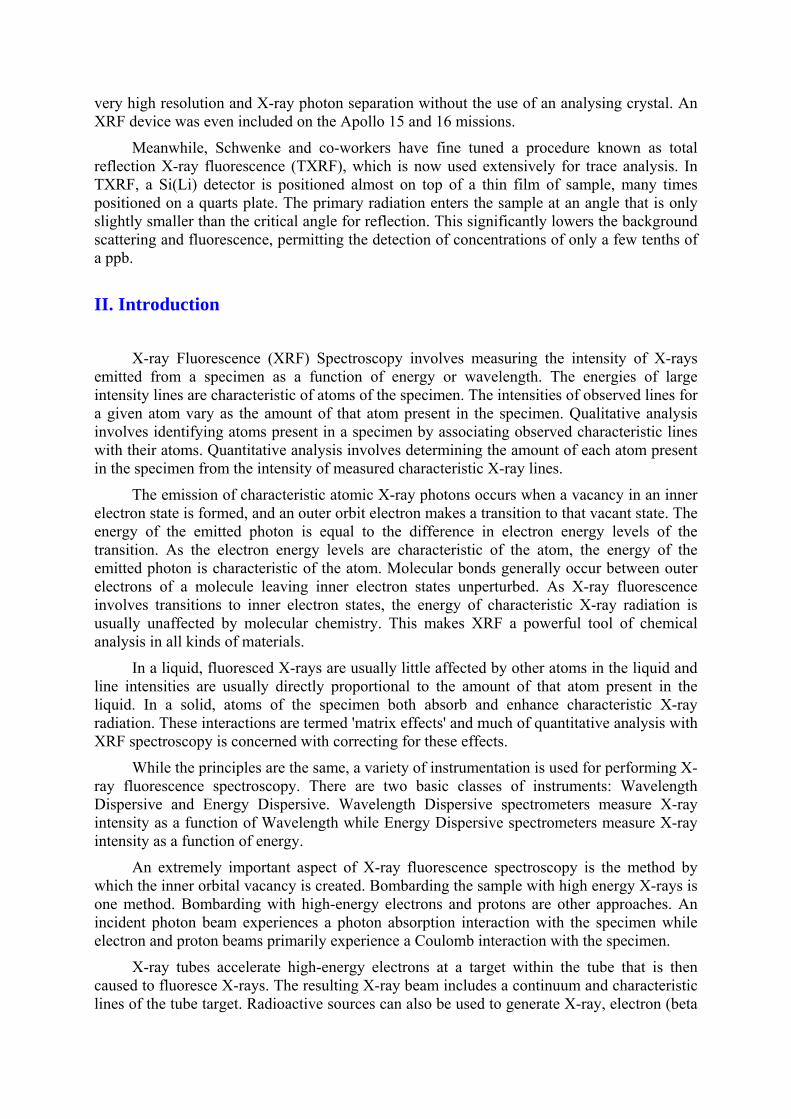
The emitted spectrum consists of the continuum (Bremsstrahlung) and superimposed are the characteristic lines of the anode material (e.g, Mo Kα and Mo Kβ) (see Figure III.5).

Figure III.5: Measured primary spectrum of a fine-focus Mo diffraction X-ray tube (45 kV acceleration voltage) as typically used for TXRF. The characteristic Mo Kα and Mo Kβ lines are superimposed on the Bremsstrahlung background.

Monochromators also can modify the primary radiation and they are usually set to the angry of the most intense characteristic line of the anode material. For a Mo-anode X-ray tube Mo Kα or for a W-anode W-Lβ are selected, but a part of the continuum can be monochromatized as well. Commonly used crystal monochromators have the disadvantage of a very narrow energy band transmitted (usually in the range of few electron volts), whereas synthetic multilayer structures are characterized by higher ∆E/E and reflectivities of up to 75 % for premium quality materials.

IV.2 Sample Reflectors

For the trace analysis of granular residues, a carrier with high reflectivity that serves as a totally reflecting sample support is required. Therefore, the mean roughness should be in the range of only a few nanometers and the overall flatness should be typically be less than λ/20 (λ = 589 nm, the mean wavelength of the visible light). Furthermore, reflectors should be free of impurities so that the black spectrum should be free from contamination peaks and the carrier material must not have fluorescence peaks in the spectral region of interest. In addition, the carrier material must be chemically inert (also against strong chemicals, which are often used for the sample preparation), easy to be cleaned for repeated use.

Some of the reflector materials that are in use are: quartz glass (most common), silicon, germanium, glassy carbon, niobium, boron nitride and (as cheapest material) Plexiglas. The requirements for the reflector are: no interfering fluorescence or diffraction lines, high purity, chemical resistance, hardness, machineability for polishing and an acceptable price. The surface must be flat and the mean roughness in the range of nanometers. Usually, they are disk shaped, with 30 mm diameter and 3 – 5 mm thickness, but also squares of 30 mm side length and rectangular types are in use.

IV.3 Detectors

Total reflection XRF is an energy dispersive XRF method, the radiation is measured mainly by Si(Li) detectors. A good detector offers a high energy resolution [Full Width at Half Maximum (FWHM) in the range of 140 eV at 5.89 keV], intrinsic efficiency close to 1 for the X-ray lines of interest, symmetric peak shapes, and low contribution to the background. Primarily, incomplete charge collection at the electrodes leads to low-energy tailing. The detector escape effect creates escape peaks and thus an increased background in certain spectral regions. An inherent advantage of semiconductor detectors is the possibility of bringing the detector crystal very close to the sample, which results in a large solid angle. Light elements emit fluorescent lines in the range from 100 to 1000 eV. The usually used Be entrance window would completely absorb them, so new window materials, offering better transmission characteristics, are used instead.

V. Quantification

One of the inherent advantages in TXRF is that one deals with thin samples so the simple conversion of fluorescent intensities I into concentration data C is applicable, as there is a linear correlation between I and C. After establishing a calibration curve either from known multielement standards or by using the fundamental parameters to calculate the calibration curve theoretically, the conversion of I into C can be immediately performed. The addition of one element as internal standard of known concentration into the sample is recommended to improve the accuracy of the results, because in this case geometric and volumetric errors will cancel. The simple relation to calculate the concentration of the unknown is given:

stdstd

std

x

xx C

IS

SIC ⋅⋅= ; (III.3)

Cx: Concentration of unknown, Cstd: Concentration of Standard, Ix: Intensity of standard, Istd: Intensity of Standard, Sx: Sensitivity of unknown, Sst: Sensitivity of Standard.

A sample is “thin” if its thickness does not exceed the critical thickness, which about 4 µm for organic tissue, 0.7 µm for mineral powders, and 0.01 µm for metallic smears. Under the assumption that the matrix absorption for the analyte differs only slightly from that of the internal standard element, these values can be generally be higher by a factor of 40 – 400. For the calculation of these values, the standing-wave field was not taken into account. This effect and the sample self-absorption can lead to contradictory requirements for the sample thickness.

VI. Influence on Detection Limits

The advantages of excitation in total reflection geometry are listed: 1. Efficient excitation by both, the primary and the reflected beam- the fluorescent signal is

doubled compared to standard excitation geometries 45° incident - 45° emission angle. 2. The spectral background caused by scattering on the substrate is reduced because the

primary radiation scarcely penetrates into the reflector substrate (high reflectivity, low transmission into the material). The scatter contribution from the sample itself is a minimum because of the 90 degree condition between incident and scattered radiation towards the detector.

3. The detector is mounted closely to the sample of small amounts are required. The samples must be prepared in aware that thin film approximation is applicable. Therefore no absorption occurs and a linear correlation between intensity and concentration of the element is valid.

4. Simultaneous multielement determination is possible due to the use of energy dispersive detectors.

Due to the argument 1 and 2 automatically the peak to background ratio is increased compared to standard XRF.

Improvements in the detection limits can be expected if the physical parameters influencing the minimum detection limits are optimised. The generally accepted definition is:

tI

S3m B

min ⋅= ; (III.4)

S: sensitivity (cps/ng); Ib: background intensity (cps); t: live time (s).

The sensitivity depends upon: 1. The intensity, respectively the brightness of the primary radiation; 2. The distances source to sample and sample to detector; 3. The detector active area; 4. The electronics in use to process the incoming countrate; 5. The insertion devices in the primary beam path to modify the spectral distribution of the

exciting radiation, improving the background but reducing the primary intensity.

The background intensity depends upon: 1. The primary intensity, its spectral distribution and the respective scattering cross

sections for the sample; 2. The sample mass (for thin film samples); 3. The geometric form and the material of the substrate and the reflection coefficient

which is practically 1. 4. Measuring in air leads to scatter of the primary radiation and contribution from

characteristic radiation of air (Ar and Kr); 5. The actual adjusted angle of incidence; 6. Solid angle of the detector;

The live time t should be chosen according to practical and economical reasons.

From the physical point of view, the sensitivity S can be influenced drastically by the proper choice of the source and its intensity, energy and beam size.

VII. General Sample Preparation

The detection limits obtained for a special sample depend very much on the sample preparation. Figure III.6 gives an overview of various common methods for sample preparation in TXRF, depending on the kind of sample to be analysed. Of course, one has to be aware that sample preparation can cause loss of elements as well as contamination by other elements and the sample taken for analysis must represent the whole specimen; therefore, homogenisation might be required.

Figure III.6: Sample preparation methods in TXRF.

Solid samples can be crushed and then ground to a fine powder of micrometer grain size. This powder can be mixed with a liquid to produce a suspension, which can be pipetted after adding an internal standard on the sample reflector. The pulverized sample can also be dissolved in a suitable solvent, and after adding the internal standard, an aliquot is pipetted on the sample reflector and dried (Figure III.7).

Figure III.7: Preparation steps for the TXRF analysis of liquids.

For the decomposition of biological and environmental materials, various methods have been utilized (e.g. with a low-temperature oxygen plasma asher, followed by dissolving the ash in an acid). The most popular method of decomposition of biological and environmental samples like plants, tissue, sediments, and so forth is the wet digestion in Teflon vessels (Teflon bombs) with acids like HNO3, HF, HNO3+HCl, HNO3+H2O2; and so forth, in different proportions. Using the hydrofluoric acid might be a problem if quartz glass reflectors are used. The use of microwave oven for heating the Teflon bomb reduces the time of digestion to less than 1 h.

The volume of some sample solutions or any sample containing water can be reduced by freeze-drying. The sample is frozen and the solvent is evaporated under vacuum conditions. The dried residue can be dissolved in small volume of acid or wet digested.

It is also possible to extract traces of certain elements by phase separation. To a given volume of sample water solutions at appropriate pH and spiked with internal standard, an organic solvent is added and mixed thoroughly. Then, the two phases are separated. The traces of metal ions stay in the organic phase, whereas the matrix elements are left in the inorganic solution. The organic liquid can be directly pipetted onto the reflector. Also, the separation of traces by adding a chelating agent and precipitating the metal ions is commonly used technique. The metal complexes are filtered through a membrane filter and dissolved in a suitable organic solvent.

VIII. Application of TXRF

Three main advantages characterize TXRF: simultaneous multielement capability, low detection limits for many elements, and small sample volume. Additional advantages are the absence of matrix effects, easy calibration, fast analysis, and comparatively low costs. Table

III.1 gives an overview of various kinds of sample that have been already analysed with TXRF. Generally all kinds of aqueous or acidic liquids where the liquid matrix can be evaporated, leaving a small amount on a sample reflector, can be analysed. Oils, alcohols, whole blood, and blood serum can be analysed after special treatment.

Table III.1: Applications of TXRF.

Environment Water Rain, river, sea, drinking, waste. Air Aerosols, airborne particles, dust, fly ash Soil Sediments, sewage sludge Plant material Algae, hay, leaves, lichen, moss, needles, roots, wood

Foodstuff Fish, flour, fruits, crab, mussel, mushrooms, nuts, vegetables, wine, tea

Various Coal, peat

Medicine/Biology/Pharmacology Body fluids Blood, serum, urine, amniotic fluid Tissue Hair, kidney, liver, lung, nails, stomach, colon Various Enzymes, polysaccharides, glucose, proteins, cosmetics, biofilms

Industrial/Technical Surface analysis Water surfaces Implanted ions Thin films Oil Crude oil, fuel oil, grease Chemicals Acids, bases, salts, solvents Fusion/Fission research Transmutational elements Al + Cu, Iodine in water

Geology/Mineralogy Ores, rocks, minerals, rare earth elements

Fine arts/Archaeology/Forensic Pigments, painting, varnish Bronzes, pottery, jewellery Textile fibres, glass, cognac, dollar bills, gunshot residue, drugs, tapes, sperm, finger prints

SECTION IV

WAVELENGTH DISPERSIVE X-RAY FLUORESCENCE (WD-XRF)

I. Introduction

Wavelength Dispersive X-Ray Fluorescence Spectrometry (WD-XRF) is the oldest method of measurement of X-rays, introduced commercially in the 1950’s. This name is descriptive in that the radiation emitted from the sample is collimated with a Soller collimator, and then impinges upon an analyzing crystal. The crystal diffracts the radiation to different extents, according to Bragg’s law, depending upon the wavelength or energy of the X-radiation. This angular dispersion of the radiation permits the sequential or simultaneous detection of X-rays emitted by elements in the sample. Simultaneous instruments normally contain several sets of analyzing crystals and detectors; one is adjusted for each desired analyte in the sample. These instruments tend to be very expensive, but efficient for the routine determination or preselected elements.

WD-XRF is a technique that has become indispensable when fast, accurate elemental analysis is needed, as when controlling a melt in a steel works or the raw mix at a cement plant. One reason for its popularity in these applications is that its ease of use, and the ruggedness of the equipment, allows quality results to be obtained in plant conditions by operators without advanced analytical skills. Furthermore, its inherent precision, speed, and simplicity of sample preparation can often eliminate many of the problems encountered with solution based methods like ICP or Atomic Absorption spectroscopy.

WD-XRF spectrometers are usually larger and more expensive than other spectrometers. Because the analyzing crystal d-spacing determines wavelength sensitivity, they are usually more sensitive than other spectrometers. To overcome losses in X-ray optics of the WD-XRF spectrometers and to maximize primary radiation intensity, X-ray tubes are usually employed. The sample is usually held under vacuum to reduce contamination and avoid absorption of light element characteristic radiation in air.

Typical uses of WD-XRF include the analysis of oils and fuel, plastics, rubber and textiles, pharmaceutical products, foodstuffs, cosmetics and body care products, fertilizers, minerals, ores, rocks, sands, slags, cements, heat-resistant materials glass, ceramics, semiconductor wafers; the determination of coatings on paper, film, polyester and metals; the sorting or compositional analysis of metal alloys, glass and polymeric materials; and the monitoring of soil contamination, solid waste, effluent, cleaning fluids, sediments and air filters.

II. Principle of WD-XRF

WD-XRF spectrometers measure X-ray intensity as a function of wavelength. This is done by passing radiation emanating from the specimen through an analyzing diffraction

crystal mounted on a 2θ goniometer. By Bragg’s Law, the angle between the sample and detector yields the wavelength of the radiation:

2 sind nθ = λ ; (IV.1)

where: d is the d-spacing of the analyzing crystal, θ is half the angle between the detector and the sample, n is the order of diffraction.

The analyzing crystal must be oriented so that the crystal diffraction plane is directed in the appropriate direction. Figure IV.1 shows a simplified schematic of the WD-XRF spectrometer. A scintillation or flow-proportional detector usually measures the fluoresced radiation. The heights of the resulting pulses are proportional to energy so using a pulse height analyzer (PHA), scattered or undesired diffraction-order X-rays can be ejected. The X-ray beam is usually collimated before and after the analyzing crystal.

Each of the components showed in the Figure IV.1 were be described in the following sections.

Figure IV.1: Schematic description of WD-XRF principle.

II.1 Collimator Masks

The collimator masks are situated between the sample and collimator and serve the purpose of cutting out the radiation coming from the edge of the cup aperture (Figure IV.2). The size of the mask is generally adapted to suit of the cup aperture being used.

The masks perform one of the two functions: background reduction and improved fluorescence (Figure IV.3).

Figure IV.2: Use of Cu 200 µm filter for cutting off the radiation coming from Rh X-ray tube.

Figure IV.3: Use of Al 100 µm filter for improvement of the ratio peak/background.

II.2 Collimator

Collimators consist of a row of parallel slats (Figure IV.4) and select a parallel beam of X-rays coming from the sample and striking the crystal. The spaces between the slats determine the degree of parallelism and thus the angle resolution of the collimator.

A 0.077° collimator is adequate for high resolution measurement parameters. Collimators with low resolution (e.g. 1.5 -2.0°) are advantageous for light elements such as Be, B and C (Figure IV.5). Using a collimator with a low resolution increases then intensity significantly. This enables intensity to be increased without a loss in angle resolution when analyzing light elements.

Figure IV.4: Collimators with different angles of resolution.

Figure IV.5: Example of the influence of collimator resolution on the intensity of a light element.

II.3 The Analyzing Crystals

II.3.1 Bragg’s Law

Crystals consist of a periodic arrangement of atoms (molecules) that form the crystal lattice. In such an arrangement of particles you generally find numerous planes running in different directions through the lattice points (= atoms, molecules), and not only horizontally and vertically but also diagonally. These are called lattice planes. All of the planes parallel to a lattice plane are also lattice planes and are at a defined distance from each other. This distance is called the lattice plane distance “d”.

When parallel X-ray light strikes a lattice plane, every particle within it acts as a scattering centre and emits a secondary wave. All of the secondary waves combine to form a reflected wave. The same occurs on the parallel lattice planes for only very little of the X-ray wave is absorbed within the lattice plane distance “d”. All these reflected waves interfere with

each other. If the amplification condition “phase difference = a whole multiple of the wavelength” (∆λ = nλ) is not precisely met, the reflected wave will interfere such that cancellation occurs. All that remains is the wavelength for which the amplification condition is met precisely. For a defined wavelength and a defined lattice plane distance, this is only given with a specific angle, the Bragg angle (Figure IV.6).

Figure IV.6: Bragg’s Law.

Under amplification conditions, parallel, coherent X-ray light (1,2) falls on a crystal with a lattice plane distanced ‘d’ and is scattered below the angle θ (1′,2′). The proportion of the beam that is scattered on the second plane has a difference of ‘ACB’ to the proportion of the beam that was scattered at the first plane.

The amplification condition is fulfilled when the phase difference is a whole multiple of the wavelength λ. This results in Bragg’s Law:

2 sind nθ = λ ; (IV.2)

n = 1, 2, 3… Reflection order.

On the basis of Bragg’s Law, by measuring the angle θ, you can determine either the wavelength λ, and thus chemical elements, if the lattice plane distance ‘d’ is known or, if the wavelength λ is known, the lattice plane –value distance ‘d’ and thus the crystalline structure.

This provides the basis for two measuring techniques for the quantitative and qualitative determination of chemical elements (XRF) and crystalline structures (molecules, XRD), depending on whether the wavelength λ or the 2d-vale is identified by measuring the angle θ (Table IV.1).

Table IV.1: Wavelength dispersive X-ray techniques.

Known Sought Measured Method Instrument type d λ θ X-ray fluorescence Spectrometer λ d θ X-ray diffraction Diffractometer

In X-ray diffraction (XRD) the sample is excited with monochromatic radiation of a known wavelength (λ) in order to evaluate the lattice plane distance as per Bragg’s equation.

In XRF, the ‘d’-value of the analyzer crystal is known and we can solve Bragg’s equation for the element characteristic wavelength (λ).

II.3.2 Reflections of Higher Orders

Figures IV.7a and IV.7b illustrate the reflections of the first and second order of one wavelength below the different angles θ1 and θ2. Here, the total reflection is made up of the various reflection orders (1, 2 …, n). The higher the reflection order, the lower the intensity of the reflected proportion of radiation generally is. How great the maximum detectable order is depends on the wavelength, the type of crystal used and the angular range of the spectrometer.

Figure IV.7a: First order reflection: λ = 2 d sin θ1.

Figure IV.7b: Second order reflection: 2λ = 2 d sin θ2.

It can be seen from Bragg’s equation that the product of reflection orders ‘n = 1; 2; ..’ and wavelength ‘λ’ for greater orders, and shorter wavelengths ‘λ* < λ’ that satisfy the condition ‘λ* = λ/n’, give the same result.

Accordingly, radiation with one half, one third, one quarter etc. of the appropriate wavelength (using the same type of the crystal) is reflected below the identical angle θ:

1 2( / 2) 3( / 3) 4( / 4)λ = λ = λ = λ =KK

As the radiation with one half of the wavelength has twice the energy, the radiation with one third of the wavelength three times the energy etc., peaks of twice, three times the energy etc. can occur in the pulse height spectrum (= energy spectrum) as long as appropriate radiation sources (elements) exist (Figure …..).

Figure IV.8 shows the pulse height distribution of the flow counter using the example of the element hafnium (Hf) in a sample with a high proportion of zircon. The Zr Kα1 peak has twice the energy of the Hf Lα1 peak and appears, when the Hf Lα1 peak is set, at the same angle in the pulse height spectrum.

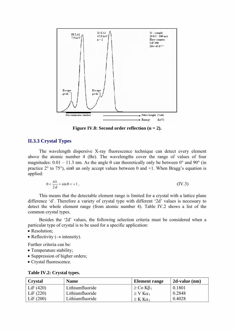
Figure IV.8: Second order reflection (n = 2).

II.3.3 Crystal Types

The wavelength dispersive X-ray fluorescence technique can detect every element above the atomic number 4 (Be). The wavelengths cover the range of values of four magnitudes: 0.01 – 11.3 nm. As the angle θ can theoretically only be between 0° and 90° (in practice 2° to 75°), sinθ an only accept values between 0 and +1. When Bragg’s equation is applied:

0 sin 12n

dλ

< = θ < + . (IV.3)

This means that the detectable element range is limited for a crystal with a lattice plane difference ‘d’. Therefore a variety of crystal type with different ‘2d’ values is necessary to detect the whole element range (from atomic number 4). Table IV.2 shows a list of the common crystal types.

Besides the ‘2d’ values, the following selection criteria must be considered when a particular type of crystal is to be used for a specific application: • Resolution; • Reflectivity (→ intensity).

Further criteria can be: • Temperature stability; • Suppression of higher orders; • Crystal fluorescence. Table IV.2: Crystal types.

Crystal Name Element range 2d-value (nm) LiF (420) LiF (220) LiF (200)

Lithiumfluoride Lithiumfluoride Lithiumfluoride

≥ Co Kβ1

≥ V Kα1

≥ K Kα1

0.1801 0.2848 0.4028

Ge InSb PET AdP TIAP OVO-55 OVO-N OVO-C OVO-B

Germanium Indiumantimonide Pentaerythite AmmoniumdihydrogenphosphateThalliumhydrogenphthalate Multilayer [W/Si] Multilayer [Ni/BN] Multilayer [V/C] Multilayer [Mo/B4C]

P, S, Cl Si Al – Ti Mg F, Na O – Si (C) N C B (Be)

0.653 0.7481 0.874 1.0648 2.5760 5.5 11 12 20

II.3.4 Dispersion, Line Separation

The extent of the change in angle ∆θ upon changing the wavelength by the amount ∆λ (thus: ∆θ/∆λ) is called “dispersion”. The greater the dispersion, the better is the separation of two adjacent or overlapping peaks. Resolution is determined by the dispersion as well as by surface quality and the purity of the crystal.

Mathematically, the dispersion can be obtained from the differentiation of the Bragg equation:

2 cosn

d∆θ

=∆λ θ

. (IV.4)

It can be seen from this equation that the dispersion (or peak separation) increases as the lattice plane distance ‘d’ declines.

II.3.5 Synthetic Multilayers

Multilayers are not natural crystals but artificially produced ‘layer analyzers’. The lattice plane distances ‘d’ are produced by applying thin layers of two materials in alternation on to a substrate (Figure IV.9). Multilayers are characterized by high reflectivity and a somewhat reduced resolution. For the analysis of light elements the multilayer technique presents an almost revolutionary improvement for numerous applications in comparison to natural crystals with large lattice plane distances (e.g. RbAp, PbST, KAP).

Figure IV.9: Diffraction in the layers (here: Si/W) of a multilayer.

II.4 Detectors

When measuring X-ray, use is made of their ability to ionize atoms and molecules, i.e. to displace electrons from their bonds by energy transference. In suitable detector materials, pulses whose strengths are proportional to the energy of the respective X-ray quants are produced by the effect of X-ray. The information about the X-ray quarts energy is contained in the registration of the pulse height. The number of X-ray quants per unit of time, e.g. pulses per second (cps = counts per second, KCps = kilocounts per second), is called their intensity and contains in a first approximation the information about the concentration of the emitting in the sample. Two main types of detectors are used in wavelength dispersive X-ray fluorescence spectrometers: the gas proportional counter and the scintillation counter.

II.4.1 Gas Proportional Counter

The gas proportional counter comprises a cylindrical metallic tube in the middle of which a thin wire (counting wire) is mounted. This tube is filled with a suitable gas (e.g. Ar+ 10% CH4). A positive high voltage (+U) is applied the wire. The tube has a lateral aperture or window that is sealed with a material permeable to X-ray quants (Figure IV.10).

Figure IV.10: A gas proportional counter.

An X-ray quant penetrates the window into the counter’s gas chamber where it is absorbed by ionizing the gas atoms and molecules. The resultant positive ions move to the cathode (tube), the free electrons to the anode, the wire. The number of electron-ion pairs created is proportional to the energy of the X-ray quant. To produce an electron-ion pair, approx. 0.03 keV are necessary, i.e. the radiation of the element boron (0.185 keV) produces approx. 6 pairs and the K-alpha radiation of molybdenum (17.5 keV) produces approx. 583 pairs. Due to the cylinder geometric arrangement, the primary electrons created in this way see an increasing electrical field on route to the wire. The high voltage in the counting tube is now set so high that the electrons can obtain enough energy from the electrical field in the vicinity of the wire to ionize additional gas particles. An individual electron can thus create up to 10.000 secondary electron-ion pairs.

The secondary ions moving towards the cathode produce measurable signal. Without this process of gas amplification, signals from boron, for example, with 6 or molybdenum with 583 pairs of charges would not be able to be measured as they would not be sufficiently discernible from the electronic noise. As amplification is adjustable via high voltage in the counting tube and is set higher for measuring boron than for measuring molybdenum. The subsequent pulse electronics supply pulses of voltage whose height depends, amongst other factors, on the energy of the X-ray quants.

II.4.2 Scintillation Counters

The scintillation counter, “SC”, used in XRF comprises a sodium iodide crystal in which thallium atoms are homogeneously distributed ‘NaI(Tl)’. The density of the crystal is sufficiently high to absorb all the XRF high energy quants. The energy of the pervading X-ray quants is transferred step by step to the crystal atoms that then radiate light and cumulatively produce a flash. The amount of light in this scintillation flash is proportional to the energy that the X-ray quant has passed to the crystal. The resulting light strikes a photocathode from which electrons can be detached very easily. These electrons are accelerated in a photomultiplier and, within an arrangement of dynodes, produce so-called secondary electrons giving a measurable signal once they have become a veritable avalanche (Figure IV.11). The height of the pulse of voltage produced is, as in the case of the gas proportional counter, proportional to the energy of the detected X-ray quant.

Figure IV.11: Scintillation counter including photomultiplier.

II.4.3 Pulse Height Analysis (PHA), Pulse Height Distribution

If the number of the measured pulses (intensity) dependent on the pulse height is displayed in a graph, we have the ‘pulse height spectrum’. Synonymous terms are: ‘pulse height analysis’ or ‘pulse height distribution’. As the height of the pulses of voltage is proportional to the X-ray quants energy, it is also referred to as the energy spectrum of the counter (Figure IV.12a and IV.12b). The pulse height is given in volts, scale divisions or in ‘%’ (and could be started in keV after appropriate calibration). The “%”-scale is defined in such a way that the peak to be to be analyzed appears at 100 %.

Figure IV.12a: Pulse height distribution

(S) Gas proportional counter. Figure IV.12b: Pulse height distribution

(Fe) Scintillation counter.

If argon is used as the counting gas component in gas proportional counters, an additional peak, the escape peak (Figure IV.13), appears when X-ray energies are irradiated that are higher than the absorption edge of argon.

Figure IV.13: Pulse height distribution (Fe) with escape peak.

The escape peak arises as follows:

The incident X-ray quant passes its energy to the counting gas thereby displaying a K electron from an argon atom. The Ar atom can now emit an Ar Kα1,2 X-ray quant with an energy of 3 keV. If this Ar-fluorescence escapes from the counter then only the incident energy minus 3 keV remains for the measured signal. A second peak, the escape peak that is always 3 keV below the incident energy, appears in the pulse height distribution.

When using other counting gases (Ne, Kr, Xe) instead of argon, the escape peaks appear with an energy difference below the incident energy that is equivalent to the appropriate emitted fluorescence radiation (Kr, Xe). Using neon as the counting gas component produces no recognizable escape peak as the Ne K-radiation, with energy of 0.85 keV, is almost completely absorbed in the counter. Also, the energy difference to the incident of 0.85 keV and the fluorescence yield are very small.

III. Points of Comparison between ED-XRF and WD-XRF

1. Resolution: it describes the width of the spectra peaks. The lower the resolution number the more easily an elemental line is distinguished from the nearby X-ray line intensities.

a. The resolution of the WD-XRF system is dependant on the crystal and optics design, particularly collimation, spacing and positional reproducibility. The effective resolution of a WD-XRF system may vary from 20 eV in an inexpensive benchtop to 5 eV or less in a laboratory instrument. The resolution is not detector dependant.

b. The resolution of ED-XRF system is dependent on the resolution of the detector. This can vary from 150 V or less for a liquid nitrogen cooled Si(Li) detector, 150 – 220 eV for various solid state detectors, or 600 eV or more for gas filled proportional counter.

Advantage of WD-XRF: High resolution means fewer spectral overlaps and lower background intensities.

Advantage of ED-WRF: WD-XRF crystal and optics are expensive, and are one more failure mode.

2. Spectral overlaps: Spectral deconvolutions are necessary for determining net intensities when two spectral lines overlap because the resolution is too high for them to be measured independently.

a. With a WD-XRF instrument with very high resolution (low number of eV) spectral overlap corrections are not required for a vast majority of elements and applications. The gross intensities for each element can be determined in a single acquisition.

b. The ED-XRF analyzer is designed to detect a group of elements all at once. The some type of deconvolutions method must b used to correct for spectral overlaps. Overlaps are less of a problem with 150 eV resolution systems, but are significant when compared to WD-XRF. Spectral overlaps become more problematic at lower resolutions.

Advantage WD-XRF: Spectral deconvolutions routines introduce error due to counting statistics for every overlap correction onto every other element being corrected for. This can double or triple the error.

3. Background: The background radiation is one limiting factor for determining detection limits, repeatability, and reproducibility.

a. Since a WD-XRF instrument usually uses direct radiation flux the background in the region of interest is directly related to the amount of continuum radiation within the region of interest the width is determined by the resolution.

b. The ED-XRF instrument uses filters and/or targets to reduce the amount of continuum radiation in the region of interest which is also resolution dependant, while producing a higher intensity X-ray peak to excite the element of interest.

Even, WD-XRF has the advantage due to the resolution. If a peak is one tenth as wide it has one tenth the background.

ED-XRF counters with filters and targets that can reduce the background intensities by a factor of ten or more.

4. Excitation Efficiency: Usually expressed in PPM per count-per-second (cps) or similar units, this is the other main factor for determining detection limits, repeatability, and reproducibility. The relative excitation efficiency is improved by having more source x-rays closer to but above the absorption edge energy for the element of interest.

a. WDXRF generally uses direct unaltered x-ray excitation, which contains a continuum of energies with most of them not optimal for exciting the element of interest.

b. EDXRF analyzers may use filter to reduce the continuum energies at the elemental lines, and effectively increasing the percentage of X-rays above the element absorption edge. Filters may also be used to give a filter fluorescence line immediately above the absorption edge, to further improve excitation efficiency. Secondary targets provide an almost monochromatic line source that can be optimized for the element of interest to achieve optimal excitation efficiency.

SECTION V

SAMPLE PREPARATION

XRF analysis is a physical method which directly analyses almost all chemical elements of the periodic system in solids, powders or liquids. These materials may be solids such as lass, ceramics, metal, rocks, coal, plastic or liquids, like petrol, oils, paints, solutions or blood. With XRF spectrometer both very small concentrations of very few ppm and very high concentrations of up to 100 % can directly be analyzed without any dilution process. Therefore XRF analysis is a very universal analysis method, which, based on simple and fast sample preparation, has been widely accepted and has found a large number of users in the field of research and above all in industry.

The quality of sample preparation in X-ray fluorescence analysis is at least as important as the quality of measurements.

An ideal sample would be prepared so that it is: • Representative of the material; • Homogeneous; • Thick enough to meet the requirements of an infinitely thick sample; • Without surface irregularities; • Composed of small enough particles for the wavelengths to be measured.

The care taken to determine the best method of sample preparation for a given material, and the careful adherence to that method, will often determine the quality of results obtained. It is safe to say that sample preparation is likely the single most important step in an analysis. A wide variety of sample types may be analyzed by X-ray spectrometer; hence, a wide variety of sample preparation techniques is required (Figure V.1).

Samples are often classified into two types based upon their thickness as measured by the attenuation of X-rays. Infinitely thick samples are those which completely attenuate X-rays emitted from the back side of the sample before they emerge from the sample. Further increase in the thickness yields no increase in observed X-ray intensity. Clearly, the critical value for infinite thickness will depend upon the energy of the emitted X-radiation and the mass absorption coefficient of the sample matrix for those X-rays.

On the other hand, a thin sample has been defined as one in which m⋅µm ≤ 0.1, where m is the mass per unit area (g/cm2) and µm is the sum of the mass absorption coefficient for the incident and emitted X-radiation. Although there are many advantages to thin samples, it is rarely feasible to prepare them for routine samples. Many samples fall between these two cases and require extreme care in preparation.

Figure V.1: Type of samples analyzed by XRF spectrometry.

I. Solids

Solid samples will be defined single, bulk materials, as opposed to powders, filings, or turnings. In many cases, solid samples may be machinated to the shape and dimensions of the sample holder. Care should be taken that the processing does not contaminate the sample surface to be used for analysis. In other cases, small parts and pieces must be analysed as received. Often, it is found useful to make a wax mold of the part which will fit into the sample holder. Using the mold as a positioning aid, other identical samples may be reproducibly placed in the spectrometer. This technique is especially useful for small manufactured parts.

Samples taken from unfinished, bulk material will often require surface preparation prior to quantitative analysis. Surface finishing may be accomplished by use of a polishing wheel, steel wool, or belt grinders with subsequent polishing using increasingly fine abrasives. Surface roughness less than 100 micrometers is usually sufficient for X-ray energies above approximately 5 keV, whereas surface roughness of less than 20–40 micrometers is required for energies down to approximately 2 keV.

II. Powders and Briquets

Powder samples may be received as powders, or prepared from pulverized bulk material which is too inhomogeneous for direct analysis. Typical bulk samples which are pulverized prior to analysis are ores, minerals, refractory materials, and freeze-dried biological tissues. Powders may be presented as such to the spectrometer, or pressed into pellets or briquets. Also, they may be fused with flux such as lithium tetraborate. The fused product may be

reground and pressed or cast as a disk. For precise quantitative determinations, loose powders are rarely acceptable, especially when low energy X-rays are detected. Pressed briquets are much more reliable.

Briquets or pressed powders yield better precision than powder samples and are relatively simple and economical to prepare. In many cases all that is needed is a hydraulic press and a suitable die. In the simplest case, the die diameter should be the same as the sample holder so that the pressed briquets will fit directly into the holder. The amount of pressure required to press a briquet which yields maximum intensity depends upon the sample matrix, the energy of the X-ray to be used, and the initial particle size of the sample. Therefore, prior grinding of the sample to a small particle size (< 100 micrometers) is advisable. In cases of materials which will not cohere to form stable briquets, a binding agent may be required. A wide, variety of binding agents have been used such as: powdered cellulose, detergent powders, starch, stearic acid, boric acid, lithium carbonate, polyvinyl alcohol and commercial binders.

III. Fused Materials

Fusion of materials with a flux may be done for several reasons. Some refractory materials cannot be dissolved, ground into fine powders, or otherwise put in a suitable, homogeneous form for X-ray spectrometric analysis. Other samples may have compositions which lead to severe interelement effects, and dilution in the flux will reduce these. The fused product cast into a glass button, provides a stable, homogeneous sample well suited for X-ray measurements. The most severe disadvantages to fusion techniques are the time and material costs involved, and the dilution of the elements which can result in an order of magnitude reduction in X-ray intensity. However, when other methods of sample preparation fail, fusion will often provide the required results.

More common are the glass-forming fusions with lithium borate, lithium tetraborate or sodium tetraborate. Flux to sample ratios range from 1:1 to 10:1. The lithium fluxes have lower mass absorption coefficients and, therefore, less effect on the intensity of the low energy X-rays. Lithium carbonate may be added to render acidic samples more soluble in the flux, whereas lithium fluoride has the same effect on basic sample. Lithium carbonate can also reduce the fusion temperature. Oxidants such as sodium nitrate, potassium chlorate or others may be added to sulfides and other mixtures to prevent loss of these elements.

IV. Filters and Ions-Exchange Resins

Various filters, ion-exchange resin beads, and ion-exchange resin impregnated filter papers have become important sampling substrates for samples for X-ray spectrometric analysis. Filter materials may be composed of filter paper, membrane filters (i.e., Nuclepore, Millipore), glass fiber filters, and others. Filters are used in a variety of applications.

One of the most widely used applications of filters is in the collection of aerosol samples from the atmosphere. Loadings of several milligrams of sample on the filter may correspond to sampling several hundred cubic meters of atmosphere. Many elements may be determined directly o these filters by X-ray spectrometric analysis.

Filters may also be used for non-aerosol atmospheric components such as reactive gases. Filter materials may be impregnated with a reagent reactive to the gas which will trap it chemically.

V. Thin Films

Thin film samples are ideal for X-ray spectrometric analysis. The X-ray intensity of an infinitely thin sample is proportional to the mass of the element on the film, and the spectral intensities are free of interelement and mass absorption coefficient effects. However, in practice, perfect thin film samples are difficult to encounter. Powder samples of sufficiently small and homogeneous particle size may be distributed on an adhesive surface such as Scotch tape, or placed between two drum tight layers on Mylar film mounted on a sample cup.

More important thin film types are platings and coatings on various substrates. Analysis of these sample types is of increasing importance for the electronics industry.

VI. Liquids

Although X-ray spectrometry is relatively unique in its ability to perform qualitative and quantitative elemental determinations on solid samples, liquids may also be analyzed. The design of X-ray spectrometric instrumentation using what has become known as inverted optics, in which the specimen is above the X-ray source and detector, facilitates the use of liquid samples. This convenient geometry demands caution in the preparation of liquid samples so that spills, leaking sample cups, and other accidents do not damage the source or detector.

Liquid samples have the excellent advantage that quantitative standards are easily prepared. However, they have the disadvantage that because solvents are usually composed of low atomic number elements, the Rayleigh and Compton scatter intensity is high; this increases background and leads to high limits of detection. Fortunately, the problems can be minimized by use of suitable primary tube filters. These reduce the scattered X-radiation in the analytically useful region. Care must be taken with liquids which contain suspended solids. If the suspension settles during the measurement time, the X-ray intensity of the contents of the sediment will be enhanced. The X-ray intensity from solution components or homogeneous suspension may decrease as a result of sediment absorption, which leads to erroneous results. This possibility is tested by taking repetitive measurements for short time periods, beginning immediately after a sample is prepared. Any observed increase or decrease in intensity with time is an indication of segregation in the sample. In these cases, an additive may be used which stabilizes the suspension, or the suspended content may be collected on a filter for analysis. Liquid samples should be considered as viable candidates for X-ray spectrometric analysis.

SECTION VI

QUANTITATIVE ANALYSIS

The observed photon rate from an analyte element in a specimen is a function of many factors including the concentration (weight fraction) of the element, the matrix (accompanying element), the specimen type (bulk, powder, liquid, thin film structure, etc.), size, preparation, geometrical set-up, spectral distribution of the exciting radiation, and the detection system. Theoretical as well as empirical approaches are used to determine concentrations from florescent intensities.

The theoretical methods are based on mathematical models for the excitation of atoms and subsequent relaxation processes, the absorption of radiation within the specimen, and the inter-element effects. Compared to a real set-up, simplifying assumption are made, for example that the specimen is perfectly flat and homogeneous, and that the incident primary beam is parallel.

An alternative is the empirical parameter method, which employs relatively simple mathematical descriptions of the relationship between photon counts and concentration (calibration curves). The general principle is that the ideal calibration curve is assumed to be a linear function, which is obtained from the (non-linear) experimental relationship by applying a number of corrections. The coefficients, by which the extent of the various corrections is introduced, are called empirical parameters. They are determined experimentally from calibration standards or sometimes by theoretical approaches.

Many times in both methods count-rate ratios (relative intensities) rather than absolute counts are used. By building ratios of the ratios of the count rate from a line of an element with the one from the same element in another specimen (which can be a standard, containing this element, or a pure element), many geometrical factors, the detection efficiency and the absolute intensity level of the primary radiation cancel.

I. Detection Limits

The limit of detection is the lowest concentration level that can be determined to be statistically significant from an analytical blank. The limit of detection is expressed as a concentration or an amount and is derived from the smallest measured value x.

The standard deviation s for counting of photons emitted at complementary random intervals of time t obeys for an average number of accumulated counts N the equations:

N Nσ = , (VI.1)

following the Poisson statistics.

Figure VI.1 shows evaluation of background.

Figure VI.1: Schematic view of net peak and background definition.

Assuming a confidence level of 95 % the total deviation is given by 2σ. The standard deviation from peak and background is assumed to be equal:

2 2 22T P B Bσ = σ + σ = σ

2 22 2 2 3 3T B B BLLD N= σ = σ ≈ σ =

3 3 3B B B

N N

N I t ILLD m m

N I t S t⋅ ⋅ ⋅

= ⋅ = ⋅ = ⋅⋅

with NS I m= , (VI.2)

generally normalized to 1000 s measuring time.

The detection limit is a method to compare the power of different analytical methods of trace element determination. Generally detection limits are derived from single element samples, so no line interference is considered. They are idealized and extrapolated values and one has to multiply these values by about a factor of 3 to come to the minimum measurable amount in real sample, but these values are good to compare different analytical methods for trace element determination.

Table VI.1 shows a comparison of detection limits in µg/cm2 for WD-XRF of Nuclepore filters and for secondary target EDXRF of Teflon filters.

Table VI.1: Comparison of Detection Limits for WDXRF and EDXRF of filter materials.

Detection Limit Detection Limit Element WDXRF EDXRF Element WDXRF EDXRF Na 310 Ge 3 Mg 60 As 4 Al 6.7 130 Se 2 Si 16 45 Br 16 2 P 8.2 Rb 3 S 5.6 15 Sr 20 3 Cl 2.2 13 Zr 8 K 3.1 6 Mo 5 Ca 1.2 5 Ag 5 Ti 4.3 30 Cd 7.5 (Lα) 6 V 1.6 20 In 6

Cr 1.2 16 Sn 4.8 (Lα) 8 Mn 2.6 12 Sb 7.1 (Lβ) 8 Fe 2.2 12 Te 10 Co 6.0 I 13 Ni 6.0 5 Cs 24 Cu 4.8 6 Ba 5.1 (Lα) 40 Zn 5 Hg 7 (Lα) Ga 4 Pb 21 (Mα) 8 (Lα)

II. Disturbing Effects

II.1 Interelement Radiation

By the term “interelements” we mean those elements in the sample which become excited together with the wanted element under the influence of the primary radiation of the source. The fluorescent radiation of interelements may disturb X-ray fluorescence determination of the element of interest, or even make it completely impossible. These disturbing effects can be classified as follows:

1. The K-series peak of the wanted element partially overlaps the K-series peaks of interelements. Remember that if the difference between the atomic numbers of two elements is lower than 3 (∆Z < 3), their characteristic peaks can be separated only by means of a solid-state detector (Si(Li)) or appropriate absorption-edge filters.

2. The K-series peak of the wanted element overlaps the L-series peaks of some of the interelements. As an example, let us consider zinc determination (ZnKα = 8.64 keV) in a sample which also contains tungsten (WLα = 8.39 keV). From the energy values of the ZnKα and WLα lines it is evident that the complete separation of two peaks may be a hard task even if a solid-state detector is used.

3. The characteristic peak of the wanted overlaps the escape peaks of interelements. An example of such a situation is the determination of vanadium (VKα = 17.47 keV) in a sample which also contains tungsten (WLα = 8.39 keV).

It follows from these examples that the choice of optimum measurement conditions for X-ray fluorescence determination of a particular element in a given material requires information concerning the latter’s chemical composition and expected concentration ranges of all the sample constituents in every analysed sample.

II.2 Matrix Effects

Generally speaking, the matrix effects in X-ray fluorescence analysis result from the influence of the variations of chemical compositions of the sample matrix on the fluorescent intensity of the wanted element. These effects can manifest themselves either via a difference in the absorption of both the primary and fluorescence radiations in samples of different matrix composition (absorption effect) or via an increase of the radiation intensity (enhancement effect) due to the fluorescence radiation of some of the interelements. These two phenomena will be discussed in detail in subsequent sections. The elements whose varying concentrations in the analysed samples lead to the effects mentioned above will be called disturbing elements.

Matrix effects constitute in most cases the major and the least easily removable sources of errors in X-ray fluorescence analysis, both in wavelength dispersive techniques and in energy dispersive ones.

II.2.1 Absorption Effect

This effect occurs when the variations in the matrix chemical composition result in changes of the mean absorption coefficients of both the primary radiation of the source and the fluorescence radiation of the wanted element. Note that the primary radiation beam penetrating into a sample undergoes attenuation due to photoelectric absorption which may occur not only in the atoms of the wanted element but also in the atoms of all the other matrix constituents. The net attenuation of the primary radiation in a matrix consisting of n elements as a function of the mean mass absorption coefficient m

oµ , expressed by the formula:

1

nm mo oi i

iw∑

=µ = µ ; (VI.3)

where moiµ are the mass absorption coefficients for the primary radiation of all matrix

constituents and wi are their concentrations expressed as weight fractions.

The absorption effects occurring in a matrix may either decrease or increase the intensity of the fluorescence radiation of the element under determination, depending on whether the matrix composition changes diminish or augment the mass absorption coefficient. A strong decrease of the fluorescence radiation of the wanted element will be observed if the concentrations of disturbing elements of slightly lower atomic numbers become larger.

II.2.2 Enhancement Effect

This effect involves an extra excitation of the atoms of the wanted element by the fluorescence radiation of some of the matrix elements, which in this case become interferants. An example of this phenomenon is illustrated in Figure VI.2.

Figure VI.2: Schematic illustration of secondary excitation in sample containing Cr, Fe

and Ni.

The mechanism of the enhancement effect involves retransmission of the energy of the primary radiation of the source in the form of secondary (fluorescence) radiation of interelements. The energy of this secondary radiation is just slightly higher than the absorption edge of the wanted element (Figure VI.3), the latter will be excited more efficiency than by the primary radiation of the source, whose energy is higher than that of the secondary radiation and, consequently, further from the absorption edge.

Figure VI.3: Mass absorption coefficient for chromium as a function of X-ray energy.

Note the strong absorption of Fe X-rays in chromium.

It can be seen that enhancement effects constitute a cascade of events, ach involving excitation of lighter atoms by the fluorescence radiation of heavier ones. Consequently, the intensity of the fluorescence radiation of the wanted element in a sample which also contains some heavier elements will depend on their atomic numbers and concentrations.

Quantitative theoretical analysis of the enhancement effects is a much more difficult problem than the analogous analysis of absorption effects. The contributions to the enhancement of a given X-ray line due to individual matrix elements cannot be expressed quantitatively by some appropriate coefficients, which might add together in a simple way as the mass absorption coefficients did. This phenomenon has been considered in theoretical terms by such author as Gillam and Heal (1952), Sherman (1955, 1959), Shiraiwa and Fujino (1966), and Lubecki (1970). The total intensity of the fluorescence radiation of an element excited within the sample both by the primary radiation of the source and by the fluorescence X-rays of one of the matrix elements may be expressed, in the most general manner, by the formula:

( )1of fI I S= + ; (VI.4)

where ofI is the intensity of the fluorescence radiation of the atoms excited by the primary

radiation of the source and S is the enhancement factor which depends, among other things, on the atomic number and weight fraction of the matrix element.

II.3 Particle-Size Effects

Particle size effects (grain-size effects, granulation effects) involve the dependence of the intensity of the secondary radiation from heterogeneous sample on the size of individual sample grains (particles) (Figure VI.4). These effects can only be removed by adequate

homogenization of the analysed material which is most easily done by fusing the sample or taking it into solution. Such a preparation of samples, however, makes the whole analysis complicated and time consuming.

Figure IV.4: Schematic illustration of particle size effects.

The direction of the changes in the fluorescent intensity which follow given changes in particle size depends on the ratio of the absorption coefficients for this fluorescent radiation of the particles containing the excited element (fluorescent particles) and of the matrix particles. For a rather weakly absorbing matrix, the fluorescent intensity decreases with the particles size. In strongly absorbing matrices, this relationship is just the opposite (Figure IV.5).

Figure IV.5: Variation in the fluorescent X-ray intensities versus diameter of the sample

grains; 1- weak absorption of fluorescent radiation in light matrix, 2- strong absorption of fluorescent radiation in matrix containing heavy elements.

II.4 Mineralogical Effects

These effects are caused by the influence, on the fluorescence intensity of the wanted element, of the type of mineral in which this element occurs (Figure VI.6). These phenomena have been reported by, among other, Campbell and Thatcher (1960) for fluorescence determination of calcium in such samples as carbonate, tungstate, or phosphate. A similar effect has been reported by Bernstein (1962, 1963) in the analysis of copper ores, where the copper was in the form of chalcopyrite (CuFeS2) and connelite (CuS).

Mineralogical effect were discussed by Claisse (1957a, 1957b), who tried to explain them starting from an hypothesis according to which the fluorescence intensity would depend on the interatomic distances separating the excited atoms in the crystal lattice. This hypothesis might be corrected in those cases where any changes in the interatomic distances lead to marked variations of the crystal density, and consequently, of the linear absorption coefficient for a given radiation in the crystal. It seems, however, that the main reason for the mineralogical effects is simply the different absorption of the fluorescent radiation in the particles of minerals of different chemical composition.

Figure VI.6: Schematic illustration of mineralogical effects.

II.5 Surface Effects

In X-ray fluorescence analysis of solid samples, such as alloys, one observes some effects due to surface irregularities. These effects are caused by the influence of the surface coarseness (or surface finish) on the intensity of the detected fluorescent radiation. The coarseness of the surface may be defined quantitatively by the dimensions of the micro-irregularities, i.e., micro-protuberances and micro-cavities which occur at the sample surface. These surface effects have been studied by, among others, Gunn (1961) and Michaelis and Kilday (1962). Their occurrence may be attributed to the shielding (absorption) effects taking place in individual protuberances at the sample surface with the fluorescence radiation emerging from the sample at different angles. According to the authors cited above, the surface irregularity effects may be of importance where both the primary and secondary radiation beams are collimated.

The magnitude of the surface irregularity effects should depend on the energy of fluorescence radiation and on the chemical composition of the sample (i.e., the sample absorption coefficient). Such dependence has actually been established.

III. Mathematical Models

III.1 Sherman Equation

Use of X-ray fluorescence to determine chemical composition of unknown specimens became more common in the following decade. With this came the need to better understand X-ray absorption and enhancement. Sherman derived a more specific equation for the

fluoresced X-ray intensity from a multi-element specimen subjected to a monochromatic non-divergent incident radiation of energy E that only accounted for primary absorption:

( ) ( )( ) ( )1

1 2

,4 sin

sin sin

i i i i ii

i

C g E I ESIEE

κ µΩ=

µµπ ψ+

ψ ψ

, (VI.5)

where: Ii: Intensity of observed characteristic line of element i. E: Energy of incident radiation. Ei: Energy of the characteristic line of element i being measured. S: Irradiated surface area of specimen. Ci: Concentration of element i in the specimen. gi: Proportionality constant for characteristic line of element i. ψ1: Angle between the specimen surface and the incident x-rays. ψ2: Angle between the specimen surface and the detector. Ω: Solid angle subtended by the detector. κ(Ei,Ii): Response of instrument at energy Ei of characteristic line energy of element i. µi(E): Mass absorption coefficient of element i at incident energy E. µ(E): Total absorption coefficient of specimen at incident energy E. µ(Ei): Total absorption coefficient of specimen at characteristic line energy of element i.

Also note that: ( ) ( )j j

jE C E∑µ = µ . (VI.6)

Sherman later developed his theory to express the emitted X-ray intensity from a multi-

element specimen subjected to a polychromatic radiation source. Sherman’s theory was then further refined by Shiraiwa and Fujino:

( ) ( ) ( )( ) ( )

( ) ( )( ) ( ) ( )

( )( ) ( )

( )( )

max

1

1 2

max 1 2

1 2

1 2

1 1,

4 sin 2sin sin

sin sinln 1 ln 1

sin sinsin sin

E ii ii i i i i o j j ji jE ii iiedge

E i j j i

E i iiedge j j

EJ JSI E I C p I E dE C pEEJ J

E E EEdE

EE E EE E

∑∫ω

∫

⎧⎪ τ− −Ω ⎪= κ + ω⎨ µµπ ψ ⎪ +⎪ ψ ψ⎩

⎫⎡ ⎤⎛ ⎞ ⎛ ⎞τ τ µµψ ψ ⎪⎢ ⎥⎜ ⎟ ⎜ ⎟• + + + ⎬⎢ ⎥⎜ ⎟ ⎜ ⎟µµ µ µµ ψ µ ψ⎢ ⎥+ ⎝ ⎠ ⎝ ⎠⎣ ⎦ ⎭ψ ψ⎪

, (VI.7)

where; Ji: Jump ratio of the photoelectric mass absorption coefficient at the absorption edge for the

line of element i being measured. ωi: Fluorescent yield for the line of element i being measured. Io(E): Intensity of incident radiation at energy E. τi(E): Mass photoabsorption coefficient of element i at incident energy E. τi(Ei): Mass photoabsorption coefficient of element i at energy Ei of characteristic line

energy of element i. pi: Transition probability of observed line of element i. Ei edge: Energy of the absorption edge of the characteristic line of element i. Emax: Maximum energy of the incident radiation.

In general this equation is referred to as the Sherman equation. The sum over j is the sum over all characteristic lines of all elements strong enough to excite the observed line of element i. The first term in the above equation represents the primary absorption of the incident and characteristic line of element i in the specimen. The second term represents the secondary enhancement of the characteristic line of element i by all other characteristic lines fluoresced by the specimen. Though not included here, Shiraiwa and Fujino also gave an expression for the tertiary enhancement of the observed line of element i by all other characteristic lines in the sample.

The Sherman equation set the stage for modern X-ray fluorescence spectroscopy. In the early days of modern x-ray fluorescence spectroscopy, the computing power required to determine the integrals of equation (VI.7) was not readily available to spectroscopy laboratories. Thus efforts turned to empirical approximations to the above equations. Using Sherman’s first equation for an incident beam of monochromatic radiation (Equation (VI.5)), Beattie and Brissey showed that by taking the ratio between counts measured for element i in an unknown to the counts measured from a pure specimen of element i, a system of simultaneous equations was created:

( ) ( )

( ) ( )1 2

1 2

sin sin

sin sin

i ji

i i i j i ij jj i j ii ii

EE

C R C C C A CEE

∑ ∑≠ ≠

⎛ ⎞µµ⎜ ⎟+⎜ ⎟ψ ψ

= + = +⎜ ⎟µµ⎜ ⎟+⎜ ⎟ψ ψ⎜ ⎟⎝ ⎠

, (VI.8)

1jjC∑ = . (VI.9)

By measuring the intensity ratios Ri for a set of standards of known composition, this system of equations could be solved for each element in the substance to determine the constants Aij.

The appearance of Ci on both sides of Equation (VI.9) meant that the system of equations had to be solved numerically. Observing that concentration was roughly proportional to measured x-ray intensity, Lucas-Tooth and Pyne rearranged the above equation to yield:

1i i i i ij jj

C a b I k I∑⎛ ⎞

= + +⎜ ⎟⎝ ⎠

. (VI.10)

Once the parameters ai, bi, and kij had been determined using a set of standards, the concentration could be determined directly from this equation for each element in the specimen. Though limited in accuracy away from concentrations of the standards used to determine the coefficients, this method was highly attractive in the days before inexpensive laboratory computers.

III.2 Empirical Alpha Models

A problem with the formulation of Beatie and Brissey was that the system of equations had no constant terms and so was over-determined. In the mid sixties, LaChance and Traill made the rather obvious observation that if Equation (VI.9) is substituted into Equation (VI.8), the over-determination of the system of equations was removed. This equation became the basis for the empirical alphas equations that followed:

1i i ij jj i

C R C∑≠

⎛ ⎞= + α⎜ ⎟

⎝ ⎠. (VI.11)

Later attempts were made to find an empirical equation that more accurately accounted for the real relationship between measured X-ray intensity and specimen concentration. Claisse and Quintin took the original Sherman equation (Equation VI.5) and modeled for polychromatic incident radiation by taking the superposition of mass absorption coefficients at multiple energies.

Though there is no direct theoretical support of this, it was generally found that the LaChance and Traill equation accounted for minor enhancement of X-ray intensities with negative alpha coefficients. Rasberry and Heinrich observed that strongly enhancing elements in binary mixtures yielded a concentration/intensity plot that did not follow the hyperbolic dependence of the LaChance and Traill equation. This led them to propose a modified form of the equation where a new term was to be used in place of the LaChance and Traill alpha coefficient for analytes causing significant secondary enhancement:

11

ij ji j

i i ij ji j i

CC R C

C

∑≠

∑≠

β⎛ ⎞⎜ ⎟= + α +⎜ ⎟+⎜ ⎟⎝ ⎠

. (VI.12)

By the middle of the seventies, other forms of the alpha correction models had been proposed. Most notable are the equations of Tertian who, observing that alpha coefficients are more properly not constant with specimen composition, proposed forms of the LaChance and Traill, and Rasberry and Heinrich equations utilizing alpha coefficients that were linear functions of element concentration Ci. Later, Tertian also showed that for a binary system, his modified form of the Rasberry and Heinrich equation reduced to the Claisse and Quintin equation.

III.3 Fundamental Parameters Method

Sherman’s equation (Equation VI.7) expresses the intensity of a characteristic X-ray fluoresced from an element contained in a specimen of known composition. By determining the concentrations of elements required to produce the measured set of intensities the composition of a specimen can be determined. The direct use of Sherman’s equation is termed ‘the fundamental parameters method’. Instrument and measurement geometry effects are removed by measuring characteristic line intensities emanating from standards of known composition. Since this equation accounts for all absorption and enhancement, in theory only one standard is required for each element. It should be noted that the standard should also account for reflection from the surface of the specimen. As such, the surface texture of the standard should be similar to that of the unknown.

Equation (VI.7) requires a knowledge of all elements contained in the specimen, the values of the total mass absorption and mass photoabsorption coefficients of each of these elements, and the step ratios of the mass photoabsorption coefficients at the absorption edges of the measured characteristic lines. A knowledge of the incident X-ray tube intensity distribution is also required. To account for secondary enhancement in the specimen, a knowledge of shell fluorescent yields and line transition probabilities are required.

Criss and Birks were among the first to utilize the full fundamental parameters method. They were able to obtain uncertainties in concentrations for nickel and iron-base alloys between 0.1% and 1.7%. Aside from the requirement for significant computing power to evaluate the above integrals, the method is limited by the accuracy of the fundamental parameters themselves, and how well the tube spectrum is known. Determining a tube spectral distribution is no trivial matter. Due to the intensity of the primary radiation, direct measurement is not feasible. A common approach was to measure the reflected distribution

from sugar, but then this involved properties of reflection. In the original Criss and Birks paper, the measured spectra of Gilfrich and Birks were utilized. Later developments either continued to use the spectra of Gilfrich and Birks, allowed user-entered spectra which usually implied the use of the spectra of Gilfrich and Birks, or utilized Kramer’s Law to generate the spectrum.

The need for computing power sufficient to evaluate the above integral and the lack of good knowledge of the tube spectrum led a number of authors to the use of an effective incident wavelength in place of the actual tube spectral distribution. Comparisons between fundamental parameters software packages utilizing effective wavelength and tube spectral distributions have demonstrated the shortcomings of this approach.

The strength of the fundamental parameters method is that only one standard is required. Since the method predicts the degree of correction for a given composition, a single standard should be sufficient for all ranges of composition of an unknown specimen. Empirical alpha models of correction require significantly more standards, and these standards need to be of similar composition to the unknown being analyzed. Early developments of the fundamental parameters method noted that most of the fundamental parameters drop out for a pure substance. Taking the ratio between X-ray intensities measured from the unknown specimen to those measured from pure substances allowed the most direct use of the fundamental parameters method. As noted by Sherman himself, and later by Criss, Birks and Gilfrich, this tends to increase the reliance on the fundamental parameters that are known to be in error by as much as 10%. The degree of correction (and so the error in correction) is reduced by using standards similar in composition to the unknown.

III.4 Fundamental Alphas

The strength of the fundamental parameters method is that it is theoretically exact, and requires relatively few standards. Aside from the need for accurate fundamental parameters and a knowledge of the X-ray tube spectrum, the fundamental parameters method is numerically intensive, and so could take a significant amount of time to compute the composition of a specimen on early laboratory mini-computers. To take advantage of the few number of standards required by the fundamental parameters method and the relatively small computing resource needed for the empirical alphas methods, the hybrid fundamental alphas method came into being. These methods use the fundamental parameters method on larger computing facilities to compute empirical coefficients that are later used in traditional empirical alphas equations on a smaller laboratory computer.

There are different methods used to compute theoretical alpha coefficients. One approach involves computing synthetic standards using the fundamental parameters method, and then computing the empirical alphas using standard regression techniques. Another approach is to compute the empirical alpha coefficients directly from Sherman’s equation for binary systems. Rousseau proposed a new empirical alphas equation that can be more directly related to Sherman’s equation:

1

1

j ijj

i ij ij

j

CC R

C

∑

∑

+ α=

+ ρ; (VI.13)

where ρij are another set of alpha coefficients.

As noted by LaChance, the fundamental parameters method and theoretical alphas of the fundamental alphas method rely on inherently different concepts. This means that the

flexibility gained by the fundamental alphas approach implies a loss of the ability to define those coefficients explicitly from theory.

It is our opinion that with the increase in laboratory computing power available by the mid 1990’s, the need for compromise with the fundamental parameters method has vanished.

III.5 Semi-Quantitative Analysis

A throw-back to the early days of XRF spectroscopy is semi-quantitative analysis. This method of matrix correction involved simply computing the concentration of an element from the product of the unknown to standard intensity ratio with the concentration of the element in the standard. More sophisticated so-called quantitative analysis methods utilized polynomials and peak counts corrected for background. These approaches are both mathematically and theoretically simplistic, and with well-designed modern XRF software, are completely unnecessary.

EXERCICES

I. (The Photon Concept)

An FM radio station of frequency 107.7 MHz puts out a signal of 50,00 W. How many photons per second are emitted?

II. (X-Ray Production)

18 kV accelerating voltage is applied across an X-ray tube. Calculate:

i. The velocity of the fastest electron striking the target,

ii. The minimum wavelength in the continuous spectrum of X-rays produced.

Mass of electron = 9 x 10-31 kg; Charge on electron = 1.6 x 10-19 C; h = 6.6 x 10-34 Js; c = 3 x 108 m/s.

III.

An X-ray tube is operated with an anode potential of 10 kV and an anode current of 15 mA. Calculate

i. The number of electrons hitting the anode per second,

ii. The rate of production of heat at the anode stating any assumptions made and

iii. The frequency of the emitted X-ray photon of maximum energy.

e = 1.6 x 10-19 C h = 6.6 x 10-34 J.s IV.

(a) What is the threshold frequency for the photoelectric effect on lithium (We = 2.9 eV)?

(b) What is the stopping potential if the wavelength of the incident light is 400 nm?

V. (The Photoelectric Effect)

A television tube operates at 20,000 V. What is λmin for the continuous x-ray spectrum produced when the electrons hit the phosphor?

VI. (The Compton Effect)

A photon having 40 keV scatters from a free electron at rest. What is the maximum energy that the electron can obtain?

VII. (Pair Production)

How much photon energy would be required to produce a proton-antiproton pair? Where could such a high-energy photon come from?

SOLUTIONS

I.

An FM radio station of frequency 107.7 MHz puts out a signal of 50.00 W. How many photons per second are emitted?

Solution

The radio waves put out by the radio station are just EM waves. Therefore, we need to calculate the energy per photon from the wave frequency (ν = 107.7 MHz), and then determine the number of photons from the signal intensity of 50,000 Watts.

The energy of each photon is:

34 6

-26

E = h ν

6.63 10 107.7 10 J.s/s

= 7.14 10 J

−= × × ×

×

The intensity is just I = NE, where N is the number of photons. Therefore, the number of photons is:

26

INE

50.00 W/J7.14 10−

=

=×

297.00 10 photons/sN = × This is a large number of photons per second, and is expected because the station power is quite large.

II.

18 kV accelerating voltage is applied across an X-ray tube. Calculate:

iii.The velocity of the fastest electron striking the target,

iv.The minimum wavelength in the continuous spectrum of X-rays produced.

Mass of electron = 9 x 10-31 kg; Charge on electron = 1.6 x 10-19 C; h = 6.6 x 10-34 Js; c = 3 x 108 m/s. Solution V = 18 x 103 V me = 9 x 10-31 kg e = 1.6 x 10-19 C h = 6.6 x 10-34 Js

c = 3 x 108 m/s

(i)

−

−

− + + −

−

=

× × × ×⇒ = =

×

⇒ = × × ×

⇒ = ×

⇒ = × ⋅

2

19 3

31

19 3 31 1

7

4

1

1

8 10

12

2 2 1.6 10 18 109 10

2 16 10 2

64 10

mV eV

eV

V

m

m

V

s

V

V

(ii)

min

min

34 8

min 19

-11min

36.63 10 3 101.16 10 18 10

6.9 x 10 m

hceV

hceV

−

−

=λ

⇒ λ =

× × ×⇒ λ =

× × ×

⇒ λ ≈

III.

An X-ray tube is operated with an anode potential of 10 kV and an anode current of 15 mA. Calculate

i.the number of electrons hitting the anode per second,

ii.the rate of production of heat at the anode stating any assumptions made,

iii.the frequency of the emitted X-ray photon of maximum energy.

e = 1.6 x 10-19 C

h = 6.6 x 10-34 Js

Solution I = 15 x 10-3 A V = 10 x 103 V e = 1.6 x 10-19 C h = 6.6 x 10-34 Js

(i)

3 -1charge 15 10 Cssecond

−= ×

19charge 1.6 10 C

electron−= ×

3

19electron 15 10second 1.6 10

−

−×

⇒ =×

16electron 9.375 10 / secondsecond

⇒ = ×

(ii)

-3 -3

Power = V × I

Power = 10×10 × 15×10

Power 150W= Entire range of wavelengths produced gives heat.

(iii)

max

max

19 3

max 341.6 10 10 10

6.63 10

h f eVeVfh

f−

−

=

⇒ =

× × ×⇒ =

×

18max 2.4 10f Hz⇒ = ×

IV.

(a) What is the threshold frequency for the photoelectric effect on lithium (We = 2.9 eV)? The lithium emitter has a work function of We = 2.9 eV. The important thing to remember is to not get confused with the units of energy (1 eV = 1.6 x 10-19 Joules).

The threshold frequency gives the photon energy (hν) that equals the work function of the emitter (We):

152.9

4.136 10 .e

oW eVh eV s−

ν = =×

147.0 10o Hzν = ×

Note the value of Planck's constant in eV.s was used instead of J.s to ensure that the units are correct.

(b) What is the stopping potential if the wavelength of the incident light is 400 nm? The stopping potential is calculated using Einstein's Photoelectric Equation for the light wavelength λ = 400 nm. The photon energy for the incident wavelength is:

1240 . 3.10400

hc eV nmE h eVnm

= ν = = =λ

Note that a standard value of hc = 1240 eV.nm was used. Get used to using certain combinations of fundamental constants, and manipulating the value of these constants in different units. This will save a lot of time doing calculations, and will ensure that answer comes out with the correct units.

The stopping potential energy is then: 3.10 2.9s eeV h W eV= ν − = −

0.20seV eV=

Therefore, the stopping potential is VS = 0.20 Volts (and is negative by definition).

V.

A television tube operates at 20,000 V. What is λmin for the continuous x-ray spectrum produced when the electrons hit the phosphor? The minimum emission wavelength for X-ray generation is given by the Duane-Hunt Rule.

By accelerating the electron through a region of total potential V = 20,000 volts, we have given it a kinetic energy of eV = 20,000 eV = 20 keV. Therefore:

min1240 .20.000

hc eV nmeV eV

λ = =

min 0.062 nmλ =

VI.

A photon having 40 keV scatters from a free electron at rest.What is the maximum energy that the electron can obtain? The photon scattering off the electron undergoes a Compton shift. It transfers some of its energy and momentum to the electron and emerges with a reduced energy and momentum (and therefore increased wavelength λ'). The electron kinetic energy is then equal to the difference between the photon energies (by conservation of energy).

The electron will have a maximum kinetic energy when the Compton shift is largest. The maximum Compton shift occurs when cosθ is a minimum (cosθ = -1). The Compton shift is then given by:

( )1 cos 2 0.0486co

h Angstromsm c

∆λ = − θ = λ =

Where λC is the Compton wavelength (λC = 0.0243 Angstroms).

The incident photon wavelength is: 1240 . 0.031 0.31

40000hc eV nm nm AE eV

λ = = = =

The scattered photon wavelength is then λ'= λ + ∆λ = 0.31+ 0.0286 A = 0.3386 A. The equivalent photon energy then:

1240 . 36.621 36.60.03386

hc eV nmE eV keVnm

′ = = = ≈′λ

Therefore, the maximum electron kinetic energy is: 40.0 36.6 3.4eK E E keV keV′= − = − =

VII.

How much photon energy would be required to produce a proton-antiproton pair? Where could such a high-energy photon come from? According to conservation of energy, the minimum photon energy required to produce a particle-antiparticle pair is just equal to twice the rest mass energy of the particle:

22 2 938.3 1.877pE m c MeV GeV= = × =

This energy could be obtained in a particle accelerator or a synchrotron.