1 Improving Satellite Data Estimation of Gas Flaring Volumes Year Two Final Report to the GGFR Christopher D. Elvidge, Earth Observation Group, NOAA National Geophysical Data Center, 325 Broadway, Boulder, Colorado 80305 USA. Kimberly Baugh, Benjamin Tuttle, Daniel Ziskin, Tilottama Ghosh Cooperative Institute for Research in the Environmental Sciences (CIRES), University of Colorado, Boulder, Colorado 80305 USA. Mikhail Zhizhin, Space Research Institute, Russian Academy of Science, Moscow. Dee Pack, The Aerospace Corporation, El Segundo, California. August 17, 2009 Table of Contents Improving Satellite Data Estimation of Gas Flaring Volumes ........................................... 1 Year Two Draft Report to the GGFR ................................................................................. 1 Abstract ............................................................................................................................... 2 1. Introduction ................................................................................................................ 3 2. Year Two Activities and Results .................................................................................. 4 2.1 Improve identification of gas flares. ......................................................................... 4 2.2 Intercalibration ....................................................................................................... 12 2.2.1 Lunar Calibration.............................................................................................. 13 2.2.2 Calculating the Uncalibrated Radiance ............................................................ 18 2.2.3 Calculating the VDGA ....................................................................................... 21 2.3 Examination of environmental effects on OLS observations of gas flares. ............ 26 2.3.1 Snow Effects ..................................................................................................... 27 2.3.2 Offshore Effects ............................................................................................... 29 2.4 Prototyping the integration of Monthly MODIS and ATSR / AATSR data............... 31 2.5 A Study of Modeling Flares to Reduce the Effects of Saturation........................... 36
Transcript
1
Improving Satellite Data Estimation of Gas Flaring Volumes
Year Two Final Report to the GGFR Christopher D. Elvidge, Earth Observation Group, NOAA National Geophysical Data Center, 325 Broadway, Boulder, Colorado 80305 USA. Kimberly Baugh, Benjamin Tuttle, Daniel Ziskin, Tilottama Ghosh Cooperative Institute for Research in the Environmental Sciences (CIRES), University of Colorado, Boulder, Colorado 80305 USA. Mikhail Zhizhin, Space Research Institute, Russian Academy of Science, Moscow. Dee Pack, The Aerospace Corporation, El Segundo, California. August 17, 2009
Table of Contents Improving Satellite Data Estimation of Gas Flaring Volumes ........................................... 1 Year Two Draft Report to the GGFR ................................................................................. 1 Abstract ............................................................................................................................... 2 1. Introduction ................................................................................................................ 3 2. Year Two Activities and Results .................................................................................. 4 2.1 Improve identification of gas flares. ......................................................................... 4 2.2 Intercalibration ....................................................................................................... 12 2.2.1 Lunar Calibration .............................................................................................. 13 2.2.2 Calculating the Uncalibrated Radiance ............................................................ 18 2.2.3 Calculating the VDGA ....................................................................................... 21
2.3 Examination of environmental effects on OLS observations of gas flares. ............ 26 2.3.1 Snow Effects ..................................................................................................... 27 2.3.2 Offshore Effects ............................................................................................... 29
2.4 Prototyping the integration of Monthly MODIS and ATSR / AATSR data. .............. 31 2.5 A Study of Modeling Flares to Reduce the Effects of Saturation ........................... 36
2
3. A 15 Year Record of Annual Gas Flaring Volumes. .................................................... 40 3.1 Uncertainty Analysis ........................................................................................... 40
4. Comparisons with Previous Gas Flare Volume Estimates ........................................... 42 4.1 Input Data ............................................................................................................... 43 4.2 Intercalibration ....................................................................................................... 44 4.3 Vectors .................................................................................................................... 45 4.4 Calibration ............................................................................................................... 46
5. Conclusion ..................................................................................................................... 49 References ........................................................................................................................ 50 APPENDIX A ‐ Does Pixel Saturation Matter? ................................................................... 51 A1 The Problem ................................................................................................................ 51 A2 The Polynomial Fit...................................................................................................... 53 A3 The Gaussian Fit Approach......................................................................................... 54
What value of d should be used? .................................................................................. 55 A4 The Fixed-Gain Composite Method ........................................................................... 56 A5 Histogram Extrapolation ............................................................................................. 58 A6 Percent Saturated Multivariate .................................................................................... 60 A7 Using Unsaturated Data Only ..................................................................................... 61 A8 Results ......................................................................................................................... 61 A10 Conclusion ................................................................................................................ 62 APPENDIX B - A Fifteen Year Record of Global Natural Gas Flaring Derived from Satellite Data, Energies v. 2, p. 595-622. http://www.mdpi.com/1996-1073/2/3/595
Abstract
This report summarizes the progress the Earth Observation Group has made in 2008 toward improving the estimation of gas flaring volumes from satellite observations and extends the long‐term record by adding estimations from 2007 and 2008. The results indicate that gas flaring peaked at about 172 BCM in 2005 and has declined by 34 BCM down to 138 BCM by 2008. The most significant improvement of our methodology was a comprehensive review of suspected flaresusing Google Earth imagery for visual confirmation. Other promising improvements which are not operational yet include:
An overhaul of our intercalibration method, based on lunar reflectance.
Mathematical fitting of flareimagery to get more accurate estimates of brightness when pixels are saturated.
Improved treatment of off‐shore flares, leading to more accurate volume estimates.
3
In addition we reviewed the gas flare detection capabilities of NASA’s MODIS thermal anomaly product and found fewer gas flare detections than the DMSP. The MODIS results indicate that NASA’s thermal anomaly processing could be adjusted to produce a comprehensive record of radiance calibrated gas flaring detections worldwide. This report also contains a retrospective analysis on why this estimate of global gas flaring is different from previous estimates.
1. Introduction
During year one NGDC demonstrated that it was possible to make reasonable estimates of national and global gas flaring volumes on an annual basis using data collected by the U.S. Air Force Defense Meteorological Satellite Program (DMSP) Operational Linescan System (OLS). At night the OLS collects low light images in a single broad band that straddles the visible and near infrared spectral range. The OLS uses a photomultiplier tube (PMT) to intensify the visible band signal to achieve detection limits that far exceed any other earth observing satellite system in the visible band range. Lights present at the earth’s surface are routinely detected by the system, including cities and towns, fires, heavily lit fishing boats and gas flares. Gas flares typically show up as circles of light, bright in the center and dim at the outer edges. These features are much larger than the flares, indicating that the OLS is detecting the lit up sky surrounding active flares. NGDC identified gas flaring features in a time series of annual nighttime light composites extending from 1995 through 2006, developed an empirical calibration based on reported gas flaring volumes from individual countries and a set of contributed data from individual gas flares, and produced the first global survey of gas flaring volumes based on satellite data spanning a twelve year period. In reviewing the results from the first year a set of issues were identified, which if resolved could lead to improved estimates of gas flaring volumes:
A. Errors of Omission and Commission: Since the OLS detects lights from cities and towns, industrial sites, and facilities such as airports – it was possible that some of the features NGDC had identified as gas flares were not indeed gas flares. Conversely NGDC may have missed some gas flares.
4
B. Intercalibration Errors: The OLS data in the current archive span five satellites (F10, F12, F14, F15 and F16). Each sensor is slightly different and their optical throughput tends to drop at a variable rate in flight. Because the OLS visible band has no on‐board calibration system NGDC developed a regression based empirical intercalibration based on the year‐to‐year changes observed in an area where lighting appeared to be largely stable over time. The are selected for this analysis was Sicily. The key assumption to this approach is that overall the lights of Sicily were stable over time – that there were not large changes in the type of lights, how they were shielded, and their numbers. There is no easy way to confirm or even evaluate the validity of this assumption.
C. Environmental Effects: Since the OLS detects lighting from gas flares many kilometers out from the gas flare location it is possible for the light to interact with the earth surface. This raise the possibility that OLS detected lighting from gas flares over a dark background (e.g. offshore) may be slightly dimmer. Conversely it is possible that the OLS detected lighting from gas flares over a bright background (e.g. snow covered) may be slightly brighter.
D. Other Sensors: There are several satellite based earth observing systems with a capability to detect gas flares that should also be considered as data sources for the estimation of gas flaring volumes.
In addition to investigating these issues NGDC also extended the record of national and global estimates of gas flaring volumes from DMSP data to include 2007 and 2008.
2. Year Two Activities and Results
2.1 Improve identification of gas flares.
NGDC reviewed each of the DMSP gas flaring features using higher resolution imagery available in Google Earth (GE). A link was built to allow the analyst to view a color composite of DMSP nighttime lights from three years (1992, 2000, 2007 as red, green, blue) within GE. The analyst could then switch back and forth from the DMSP view to the GE view. The base
5
imagery in GE was 30 meter Landsat and in many cases there was one meter color Digital Globe imagery available at gas flaring sites. The Landsat data in GE is from year 2000 (+/‐) while the Digital Globe imagery is much more recent (past 2‐3 years). With the Landsat data it is possible to identify cities and towns, airports, industrial facilities, and roads. In many cases an orange discoloration was found at gas flares sites in the GE Landsat imagery. Examples of gas flares identified based on Landsat imagery in GE are shown in Figure 1 (a,b,c). In the digital globe imagery it is possible to identify gas flare stacks, flare pits, and even the flames from gas flares (Figure 2 a,b,c). The analyst created placemarks to record what was found at each of the DMSP identified gas flaring features. Red placemarks were created for features that were either confirmed or consistent with gas flares (Figure 3). Green placemarks were created for cities, towns, airports, industrial sites, or mines that could be confused with gas flares. A separate set of placemarks was generated for each country. The red and green placemarks were then used to guide the drawing of gas flare vectors for each country. The GE placemarks for each country are posted for open access at: http://www.ngdc.noaa.gov/dmsp/interest/gas_flares_countries_kmz.html. The updated gas flare vectors for each country are posted in shape file format at: http://www.ngdc.noaa.gov/dmsp/interest/gas_flares.html.
6
Figure 1a. Example of a gas flaring site in Nigeria identified based on Landsat imagery in GE. Note the network of ditches and presence of production pads. Several white clouds are present. The flare site was marked at the center of the orange discoloration in the center of the image.
7
Figure 1b. Example of a gas flaring site in Iraq identified based on Landsat imagery in GE. The flare site was marked at the center of the orange discoloration in the center of the image.
8
Figure 1c. Example of a gas flaring site in Khanty‐Mansiysk identified based on Landsat imagery in GE. The surrounding area has a network of roads connecting the production pads to the central processing facility. The flare site was marked at the center of the orange discoloration found at the processing facility.
9
Figure 2a. Example of a gas flaring site in Nigeria identified in Digital Globe imagery in GE. There is a processing facility on the right with a pipeline extending out to two square shaped flare pits with flames.
10
Figure 2b. Example of a gas flaring site in Iraq identified in Digital Globe imagery in GE. There is a processing facility to the north (not shown) with a set of pipeline extending down to a series of four active gas flares.
11
Figure 2c. Example of gas flaring site in Khanty‐Mansiysk identified in Digital Globe imagery in GE. The gas flare was marked at the center of the circular flare pit to the east of the processing facility. Note the presence of a flame within the circular flare pit.
12
Figure 3. A set of placemarks was created based on a visual interpretation of the Landsat and Digital Globe imagery for each of the features identified as a gas flare in the DMSP nighttime lights data. Sites that had either clear indications of gas flaring, or no features inconsistent with being a gas flare, were marked as red. Sites which were clearly not gas flares (cities, towns, airports, mines) were marked with green placemarks.
2.2 Intercalibration
The OLS visible band lacks on‐board calibration. During year‐one NGDC developed an empirical intercalibration based on electric lighting detected in Sicily – a region where the lighting appears to have been largely stable from the early 1990’s. The objective of the intercalibration is to adjust the satellite image brightness levels to account for differences between sensors and the degradation of individual sensors over time. This initial intercalibration can be readily questioned because there is no way to verify
13
that the lights in Sicily or any other place have not changed from the 1990’s to the present.
2.2.1 Lunar Calibration
In year two we began work on an intercalibration based on the observation of large highly reflective surfaces in desert regions. This approach follows methods that date back into the 1970’s for calibrating earth observation satellite data using solar illumination reflected back into space from desert surfaces. The ideal surfaces are large, have minimal spectral variation, are cloud‐free most of the time, and have very little vegetation. For the DMSP‐OLS we are using lunar instead of solar illumination. Under full moon conditions it is possible to see many terrain features in the nighttime visible band data. Figure 4 shows White Sands, New Mexico for ten nights across a full moon. White Sands has been frequently used in this style of calibration [e.g. Che and Price, 1993].
Figure 4. DMSP OLS nighttime visible band images of White Sands, New Mexico from January 3 through January 14, 2009. White Sands is the large white spot in the January 11 (full moon) image. On nights with no
14
moonlight White Sands cannot be detected. Several lights from small towns are detected to the east and south of White Sands. We are very close to being able to run an intercalibration using this approach. The checklist and status for each item is described in Table 1.
STEP DESCRIPTION STATUS
1 Model of the incoming lunar irradiance for any specified date, time and location.
Complete. Figures 5 and 6.
2 Model of the atmospheric effects on the incoming moonlight.
MODTRAN atmospheric transmission model has been purchased and implementation has begun. See Fig 7.
3 Acquire reflectance spectra of the desert surface.
Complete. See Fig 8.
4 Model the atmospheric effects on the reflected spectrum as it passes from the surface to the detector.
In progress using the MODTRAN model.
5 Pass reflected radiation through the instrument response function.
Complete. See Fig 9.
6 Compare modeled radiance with the uncalibrated radiance in order to calibrate instrument sensitivity.
In progress. See Figs 10‐15 and discussion regarding the calculation of uncalibrated radiance (section 2.2.2).
7 Intercalibrate the results from different satellites to create a consistent long‐term record.
In progress.
Table 1. Intercalibration checklist.
15
Figure 5. Lunar irradiance spectra (top of atmosphere).
16
Figure 6. Total lunar irradiance versus time at White Sands, New Mexico.
17
Figure 7. Lunar Irradiance at the Earth’s surface modeled by MODTRAN. .
Figure 8. Average field reflectance spectrum of White Sands, New Mexico.
18
Figure 9. Normalized spectral responses on the OLS nighttime visible bands. The spectral responses of each instrument can introduce subtle differences between satellite observations (especially in the near‐IR region). These functions are measured pre‐launch and presumably do not change with time. They are one component of the system’s sensitivity to radiation. Note that the OLS was designed to observe moonlit clouds and so these spectral response functions are not optimized to measure gas flares.
2.2.2 Calculating the Uncalibrated Radiance
In order to arrive at an absolute radiometric calibration we first derive the uncalibrated radiance (i.e. what the sensor reports as the radiance). When this is compared to the “true” radiance impacting the sensor then a correction can be derived for our observations. We need the capability to predict the visible band gain state for each OLS pixel and the uncalibrated radiance per digital number for each possible gain setting. The elements now assembled for the prediction of the gain and calculation of the uncalibrated radiance include:
19
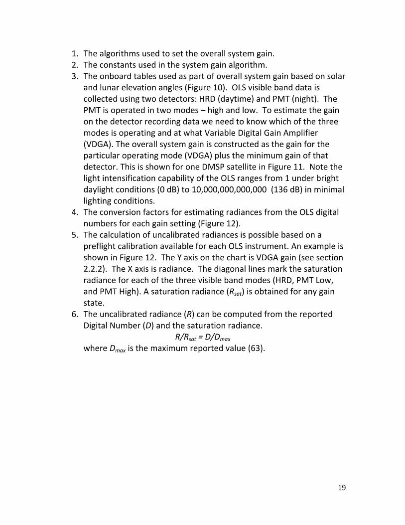
1. The algorithms used to set the overall system gain. 2. The constants used in the system gain algorithm. 3. The onboard tables used as part of overall system gain based on solar
and lunar elevation angles (Figure 10). OLS visible band data is collected using two detectors: HRD (daytime) and PMT (night). The PMT is operated in two modes – high and low. To estimate the gain on the detector recording data we need to know which of the three modes is operating and at what Variable Digital Gain Amplifier (VDGA). The overall system gain is constructed as the gain for the particular operating mode (VDGA) plus the minimum gain of that detector. This is shown for one DMSP satellite in Figure 11. Note the light intensification capability of the OLS ranges from 1 under bright daylight conditions (0 dB) to 10,000,000,000,000 (136 dB) in minimal lighting conditions.
4. The conversion factors for estimating radiances from the OLS digital numbers for each gain setting (Figure 12).
5. The calculation of uncalibrated radiances is possible based on a preflight calibration available for each OLS instrument. An example is shown in Figure 12. The Y axis on the chart is VDGA gain (see section 2.2.2). The X axis is radiance. The diagonal lines mark the saturation radiance for each of the three visible band modes (HRD, PMT Low, and PMT High). A saturation radiance (Rsat) is obtained for any gain state.
6. The uncalibrated radiance (R) can be computed from the reported Digital Number (D) and the saturation radiance.
R/Rsat = D/Dmax where Dmax is the maximum reported value (63).
20
Figure 10. On‐board look up table for the part of the system gain based on solar and lunar elevations. At night the gains can be further adjusted for the phase of the moon.
Figure 11. OLS System Gain is achieved with 3 operating modes: HRD for daytime, PMT Low near the terminator (the boundary between day and night), and PMT High for nighttime. The relationship between the operating mode gains and system gains for satellite F16 is shown here. The vertical lines indicate the switch points between the modes.
21
Figure 12. Preflight calibration of an OLS showing the saturation radiance versus gain setting for the three operating modes: HRD, PMT Low, and PMT High.
2.2.3 Calculating the VDGA
The OLS is operated to provide a relatively even brightness of nighttime clouds regardless of illumination. To serve this purpose the gain is continuously adjusted in response to solar and lunar elevation angles, lunar phase, and scan angle. Under high moon conditions (i.e. full moon at high elevation angles) the gain is suppressed. When there is little moonlight the gain is turned up. These adjustments occur continuously so that the gain varies from pixel to pixel. Figure 13 shows a portion of imagery that highlights these gain changes.
22
Figure 13. A) OLS fine resolution imagery showing the passage from night to day. B) The computed gain settings associated with this image. Note the top left corner is using the HRD detector, the lower right is using the PMT High detector, and the diagonal zone near the terminator is using the PMT Low detector. The along scan gain changes occur as the scanner encounters different scene light levels. The abrupt along track changes in gain as the satellite travels northward occur due to commanded changes in the maximum allowed system gain constant (BCMAX). The only place where the gain state is recorded in the OLS data is for the last pixel in each scanline (7324 pixels per scanline) of the fine resolution data. Since the OLS scans left to right and then back right to left the gain is available at both ends of each pair of scan lines. This value is obliterated by the 5 x 5 on‐board averaging that creates the smoothed data that form the bulk of the OLS archive. However a small fraction of the fine resolution data is transmitted to the ground and ends up in the OLS archive. In our
23
initial testing we are comparing the calculated gain against the recorded gain for the last pixel in the scanlines (See Fig 14). In Figure 14 it is possible to identify the daytime imaging collected by the HRD (High Resolution Detector), the rapid transitions (steep diagonal line segments) in gain as the scanline crosses from daylight, across the terminator and into darkness.
Figure 14: VDGA gains recovered from the last pixel in each scanline for the fine resolution data from satellite F16 from the year 2006.
While the record of gain changes are not imbedded in the data stream, we have obtained the along scan gain control (ASGC) algorithm used for the OLS, and we do have access to the gain constants via the Payload Activation Messages (PAMs). The PAMs are generated on a weekly basis and contain updates to the gain constants memories which are accessed by the
24
onboard gain algorithm. From the PAMs we are able to recover these gain constants (see Table 2):
BCMAX Maximum system gain setting
BRDFHRD Bidirectional Reflectance Distribution Function (BRDF) setting when the HRD is selected
BRDFPMT BRDF setting when the PMT is selected
BRDFX2 BRDF factor of x2 where x is a function of the source and view angles.
GAIN1 Gain offset between HRD and PMT Low
GAIN2 Gain offset between HRD and PMT1/9 (currently unused)
GAIN3 Gain offset between PMT Low and PMT High
HRDOFS HRD gain offset
LGBIAS Lunar Gain Bias
LPA Lunar Phase Gain Coefficient A
LPB Lunar Phase Gain Coefficient B
LPC Lunar Phase Gain Coefficient C
RV1 Coefficient 1 for the Diffuse Component of the BRDF correction
RV2 Coefficient 2 for the Diffuse Component of the BRDF correction
RV3 Coefficient 3 for the Diffuse Component of the BRDF correction
RV4 Coefficient 4 for the Diffuse Component of the BRDF correction
SWPT1 Switch point between HRD and PMT Low
SWPT2 Switch point between HRD and PMT1/9 (currently unused)
SWPT3 Switch point between PMT Low and PMT High
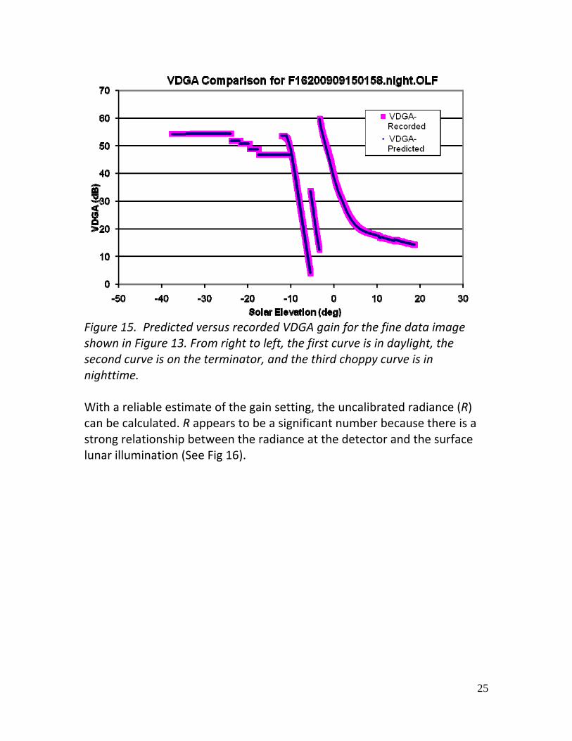
Table 2. PAM parameters. Using this information we have begun the process of simulating the gain settings for each OLS pixel in fine resolution data so that they can be compared against the values recorded in the last pixel of each scanline. Figure 15 demonstrates our progress in predicting the VDGA for imagery with a range of solar and lunar elevations.
25
Figure 15. Predicted versus recorded VDGA gain for the fine data image shown in Figure 13. From right to left, the first curve is in daylight, the second curve is on the terminator, and the third choppy curve is in nighttime. With a reliable estimate of the gain setting, the uncalibrated radiance (R) can be calculated. R appears to be a significant number because there is a strong relationship between the radiance at the detector and the surface lunar illumination (See Fig 16).
26
Figure 16. Calculated Radiance at the detector (R) as a function of Surface Lunar Illumination as estimated by a US Naval Observatory model [Janiczek and DeYoung, 1987]. The final step is to compare the uncalibrated radiance to the modeled radiance. This relationship will establish the in‐flight efficiency of each detector. Then we can scale the images appropriately for meaningful intercalibration which is independent of many of the assumptions that were present in our previous efforts. For example, we assume that our averages are of sufficiently large numbers of overpasses so that changes in gain at any location do not significantly bias our results. At present, this assumption remains untested.
2.3 Examination of environmental effects on OLS observations of gas
flares.
The visible and near‐infrared band region is susceptible to environmental effects which were not fully explored during year‐one. During year‐two we attempted to quantify the influence of earth surface brightness on the
27
detected lighting. The hypothesis to be tested was that the lights will appear smaller and dimmer when the flares are over a dark background and conversely appear to be larger and brighter when the flares are over a bright surface. NGDC conducted two types of tests: 1) comparison of snow versus no‐snow conditions, and 2) comparison of sets of onshore and offshore flares where reported BCM are available.
2.3.1 Snow Effects
The effects of snow were examined using nighttime OLS data over five separate gas flares in Kazakhstan. Kazakhstan was selected for several reasons: 1) It is at a mid‐latitude (~48 degrees north) resulting in a longer annual period of usable nighttime observation from the OLS. At higher latitudes the usable period of nighttime lights gradually reduces to the core winter months due to solar contamination. 2) There are several large gas flares present. And 3) there is wide variation in snow cover during the period when usable nighttime lights are collected. Percent snow cover was obtained from NASA, processed from data collected by the Moderate Resolution Imaging Spectrometer (MODIS). We used the daily snow cover product (http://modis‐snow‐ice.gsfc.nasa.gov/MOD10A1.html), generated by combining the MODIS data from two satellites. Because the flares differ in overall size the sum of lights index values for the five flares were normalized prior to examining for snow effects. Figure 18 shows the normalized sum of lights index values versus percent snow cover for the observations that had less than 20% cloud cover in the test areas. Linear regression came out with an R2 value of 0.00 indicating that, assuming no significant seasonal variation in flare levels, there is no discernable effect from snow on the sum of light index values.
28
Figure 17. Location of five test areas centered on gas flares in Kazakhstan. The test sites are outlined in green and are numbered one through five.
Figure 18. Normalized sum of lights index values versus percent snow cover for five gas flare sites in Kazakhstan.
29
2.3.2 Offshore Effects
Gas flares are found both on land and on platforms at sea. There is a question about whether making a distinction between these two types of flares affects the total estimate of flared gas. Several approaches were made to resolve this question. On initial inspection, there does appear to be a difference between onshore and offshore points in the calibration data (See Figure 19). The offshore flares have slightly higher reported flared gas volumes for the same sum of lights index values. This discrepancy is consistent with the physical explanation that water absorbs more of the near infrared radiation from the flare than the land.
Figure 19. Calibration data segregated by water and land. Separate regression lines are shown.
30
With the assumption that offshore and onshoreflares should be calibrated differently, the measurement of the sum of lights index was performed twice – once for onshore areas only, and the second for offshore areas only. The appropriate calibration coefficients were applied to each extraction, and the results were summed. The results were checked for Nigeria, since that country has nearly equal onshore and offshore gas flaring. Note that when the onshore and the offshore sum of lights indices were added, their sum differed from the desegregated sum of lights by less than 1%. When the estimated flaring volumes were calculated separately for land and offshore and then summed, the estimated flaring level in Nigeria was about 35% higher than reported data (which was considered to represent “the truth”). Despite the promising start therefore, this approach was abandoned. Another facet we investigated was if the background threshold we chose contributed to the land‐water distribution of calibration points. Currently, the background threshold was set to 8 digital number (DN), meaning that any value smaller than 8 was considered background lighting and not included in the integration of the flare brightness. It was noted that background lighting over water is significantly and consistently lower than 8. If the threshold over water is reduced to 2 DN then about 34% more light is integrated around the flares. This method of extraction shifts the population of water flares, so that it appears nearly indistinguishable from the onshore flares (see Figure 20). When a regression is performed on the ensemble of points, the correlation coefficient (R2) is 0.90 compared to 0.98 when onshore is regressed separately.
31
Figure 20. The recalculation of the calibration coefficient when onshore points are combined with reduced‐threshold offshore points. The results to date indicate that it may be appropriate to process the onshore and offshore gas flares differently. This has not, however, been done with the data processed to date.
2.4 Prototyping the integration of Monthly MODIS and ATSR / AATSR
data.
To date there has not been a satellite sensor optimized for the detection of gas flares and estimation of flared gas volume. Over the years we have noted several shortcomings to the DMSP data: 1) gas flares are so bright that they often saturate the DMSP visible band, 2) gas flares can only be detected at night and cannot detect flares in mid‐to‐high latitudes during the summer due to solar contamination, 3) there is no on‐board calibration for the DMSP visible band, 4) it is impossible to identify gas flares inside of lit urban centers and at more remote gas flares lighting from the facility is included in the DMSP signal, and 5) the low light imaging data may be subject to environmental effects that are difficult to account for (such as enhanced sky brightness when snow is present on the ground). These are all areas where MODIS may offer some advantage over DMSP for the estimation of gas flaring volumes:
32
MODIS is radiometrically calibrated and tends not to saturate by fire
data, allowing for the estimation of flare brightness temperatures in
many cases.
MODIS has dedicated fire bands which can resolve gas flares in lit
areas (i.e. cities).
With MODIS data thermal anomalies can be detected day or night
with no seasonal restrictions (other than cloud cover)..
MODIS may reduce inaccuracies due to environmental factors such
as cloud cover, snow, or solar contamination.
NASA collects both daytime and nighttime data from two satellites
(TERRA and AQUA).
The MODIS archive extends back to year 2000.
A follow on sensor (VIIRS) is being built by NOAA, NASA and DoD.
NASA processes the global MODIS data stream to detect fires. The obvious
shortcomings in these products for the monitoring of gas flares are that the
fire detection algorithm is only applied to onshore areas. We have visually
reviewed MODIS data in offshore gas flare locations to and found that the
sensor detects offshore flares. This observation is confirmed by a 2007
NASA report (Gallagos, 2007) which examined the detection of small gas
flares in the Gulf of Mexico. In theory it would not be difficult to extend the
fire detection processing into the offshore areas with known gas flares.
During year two we investigated the possibility that the MODIS fire
detections could be normalized for cloud‐cover, as are the DMSP nighttime
lights products used in the estimation of gas flaring volume. The issue is
that gas flares will be detected less frequently in regions having extensive
cloud cover. Gas flaring volumes would be underestimated in the cloud
33
impacted areas and overestimated in cloud‐free desert areas without
normalization for cloud‐cover differences. The same holds for areas with
lower numbers of MODIS observations.
NASA produces a combined fire detection and a cloud cover product from
MODIS data named MOD14. These products are available from the U.S.
anomalies_fire/daily_l3_global_1km/v5/terra). We downloaded one
month (January 2003) of the MOD14A 1 products for the Nigeria region and
successfully applied the cloud‐free compositing procedure developed for
DMSP nighttime lights. Figure 21 shows the MOD14A1 cloud cover map for
January 23, 2003. The DMSP cloud‐free compositing software was used to
process the MODIS data to produce two output grids: 1) the percent
frequency of fire detections, and 2) the average brightness temperature for
all the detected fires. In the percent frequency grid we found that gas
flares had much higher frequencies of detection than agricultural and other
types of biomass burning (Figure 22). DMSP data exhibit the same result,
with gas flares being persistent source of light while other types of fires are
ephemeral. Figure 22 shows the DMSP detected lights from January 2003
as blue and the percent frequency of MODIS fire detections as white. We
found that, using MODIS data, it is easy to separate the gas flares from the
other types of fires based on the high percent frequency of occurrence of
the gas flares. The MODIS detected all of the large gas flares detected by
DMSP – but was unable to detect many of the smaller flares. While none of
the offshore flares were detected by MODIS, this was expected since the
NASA algorithm ignores fires on the water.
Our conclusion regarding MODIS is that the existing MOD14 products could
be used to analyze the frequency and temperature of the larger onshore
gas flares worldwide – back to year 2000. The magnitude of such an effort
34
would be reasonable since the MOD14 products are available at no‐cost,
The MOD14 product size is compact when compared to the original MODIS
data, the locations of major gas flaring are already known, and the
relatively simple the processing has already been prototyped.
To obtain a MODIS gas flaring record of offshore flaring would require
reprocessing in areas known to have gas flares. The offshore gas flare
detection algorithms developed by Gallegos (2007) would be a good
starting point for the selection of an algorithm for the processing.
We were unable to complete the planned study on ATSR/AATSR fire
detections from the European Space Agency due to delays in the
reprocessing of the archive. The ATSR/AATSR fire detection algorithm is
only applied to the nighttime data and their cloud detection algorithm only
works on daytime data. ESA is currently reprocessing the ATSR/AATSR
archive with a uniform set of fire detection thresholds and a tracking of the
total number of coverages. We hope to work with the reprocessed
ATSR/AATSR data in 2009.
35
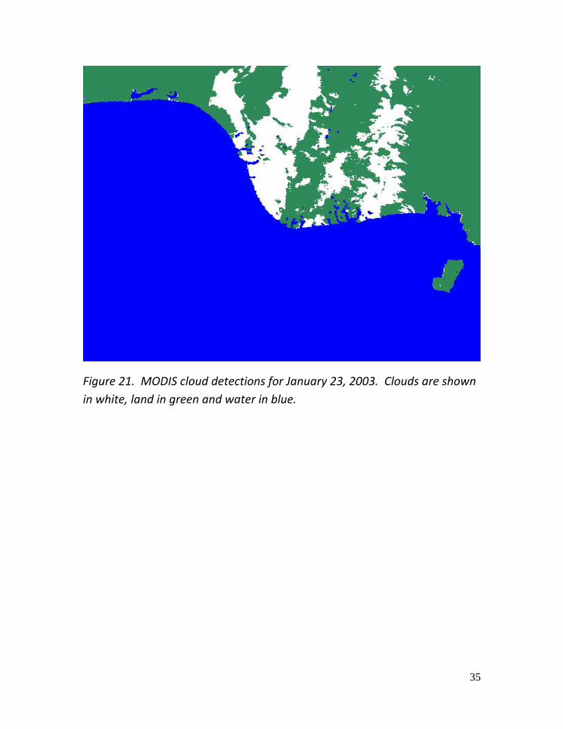
Figure 21. MODIS cloud detections for January 23, 2003. Clouds are shown
in white, land in green and water in blue.
36
Figure 22. The percent frequency of MODIS fire detections during January
2003 overlaying the DMSP detected lights from the same month (blue).
Vectors are drawn to indicate the position of the shorelines, countries, and
gas flares identified for Nigeria.
2.5 A Study of Modeling Flares to Reduce the Effects of Saturation
During year two we investigated the Gaussian modeling of the gas flares in the DMSP lights data. The main objective was to correct the sum of lights where it may be underestimated when the DMSP data are saturated. Figure 23 shows a transect across the tops of two flares, with and without saturation (values of 63). If we are successful in modeling the missing portion of the signal – lost due to saturation – this could improve the calibration and extraction used to estimate the flared gas volume. In
37
reviewing the locations of saturated data in gas flares around the world we found that the majority of flares do not have a saturation problem (see example in Figure 24).
Figure 23. Transects across the tops of two flares. The first one is unsaturated and exhibits a classic Gaussian shape. The second has saturation, with a flat top where the values are all 63’s. We attempted to model the missing part of the signal from the flares with saturation.
38
Figure 24. The nighttime lights of the gas flaring region in Nigeria region from 2008 showing areas of saturation as red. After attempting several methods of removing the bias associated with saturation, we found that most corrective measures converged on the same estimate of flaring volume as the “no correction” method. These methods are described in Appendix A – Does Saturation Matter?. The tentative conclusion we arrived at is that saturation is not a significant cause of bias in our analysis. The most compelling evidence to support this unexpected conclusion includes:
Each method converged on approximately the same estimates of gas
flaring volume (consistent with “no correction”).
The calibration dataset includes 'saturated' data to approximately
the same extent as the rest of the data, and therefore the calibration
coefficient obtained approximately corrects for under‐estimation of
saturated flares.
39
Saturated regions account for about 15% of the actual sum of lights
for each flare. Most of the information is contained in the pixels
surrounding the saturated pixels.
When the sum of lights from Fixed Gain data (as described in
Appendix A), which contains no saturated pixels, is plotted against
the 'normal gain' data which includes saturated pixels, the
relationship is linear at all scales (see Figure 25). If saturation were
affecting the sum of lights calculated from the 'normal gain' data
significantly, then regions of high saturation would be expected to
cause a “bend” in the data.
Figure 25. Sum of Lights computed from both Fixed Gain data and the
Standard Method. Note the linearity for even the highest flaring countries.
40
3. A 15 Year Record of Annual Gas Flaring Volumes. Our estimates of global gas flaring volumes are shown in Figure 26. These estimates are higher than the estimates reported during year one as a result of more gas flares having been identified based on the higher resolution imagery in Google Earth. One of the reasons we can say this with confidence is that the coefficient for estimating BCM remained approximately the same (BCM = 2.66E‐5 times the sum of lights index). In October 2008 we provided a provisional set of estimates using a slightly lower coefficient (BCM = 2.54E‐5 times the sum of lights index) based on a subset of the reported data. The results presented in Figure 26 indicate that gas flaring peaked at about 172 BCM in 2005 and has declined by 34 BCM down to 138 BCM by 2008. The DMSP satellite data show a steady decline in gas flaring volume over the past three years. The top twenty flaring countries in 2008 are listed in Table 3. The top five countries for decreases in gas flaring volume from 2007 to 2008 are listed in Table 4. The list is lead by Russia, which had an 11 BCM decline in gas flaring last year according to data from two DMSP satellites (F15 and F16).
Figure 26. DMSP estimated gas flaring volumes in billions of cubic meters (BCM). Note the error bars are in the +/‐10% range.
3.1 Uncertainty Analysis
The error estimate is derived from the calibration of the sum of lights index to the reported flaring values for countries and individual flares. This
41
regression allows us to generate a calibration coefficient that will be used to multiply the observed sum of lights to convert it to an estimate of gas flaring volume. There is uncertainty in both the reported data and the satellite observations and both contribute to error in the derivation of the calibration coefficient. We quantify this error by calculated the 95% interval around the best fit line. Within this interval 95% of the calibration points (N=397) are contained by the fit (See Figure 27).
Figure 27 Calibration Regression. Plot of the reported BCM levels of flared gas versus the sum of light index, regression line (solid line) and 95% prediction intervals for individual BCM estimates (dashed red lines). The prediction interval (σ) is then considered the uncertainty of any national estimate of gas flaring. The uncertainty is reduced by a factor of 1/√2 when we average two satellite observations. When the global total is compiled by summing the flaring of about 60 countries (N=60) then the uncertainty is propagated as √N σ.
Table 3
Top Twenty Gas Flaring Countries in 2008
COUNTRY Gas Flaring Volume 2008 (BCM)1 Russia 40.6
4. Comparisons with Previous Gas Flare Volume Estimates In 2007 NGDC issued a report which covered the years 1995‐2006, estimating the global gas flaring volumes (V1) [Elvidge et al. 2007]. In the
43
fall of 2008 a new estimate was made expanding the coverage from 2004‐2007 (V2). In May of 2009, we prepared a 2nd report [this document] including a revised estimate and expanding the temporal coverage to include 1994‐2008 (V3). The V2 global BCM estimates were slightly lower than the V1 estimates. V3 produced BCM estimates about 4% higher than V1. What contributed to the revisions?
Figure 28 – Global gas flaring by year for three different revisions. V1 is the report to the World Bank in 2007; V2 is the revision reported at the Gas Flaring conference in November 2008; and V3 is the latest revision presented in this report.
4.1 Input Data
Table 1 summarizes the additions and changes made to the series of annual cloud‐free nighttime lights composites used in the analyses. During the second year we processed data from DMSP satellite F15 and F16 to fill in and extend the record national and global flare volumes estimates. This included the processing of a full year of 2006 data from the two satellites. The year one reporting for 2006 was based on data collections from January through September 2006. The current set of annual composites for which we have estimated gas flaring volumes are listed in Table 5.
Table 5 Data Processed In Year Two Are in Red
44
Year Satellites
1994 F12
1995 F12
1996 F12
1997 F12 F14
1998 F12 F14
1999 F12 F14
2000 F14 F15
2001 F14 F15
2002 F14 F15
2003 F14 F15
2004 F15 F16
2005 F15 F16
2006 F15 F16
2007 F15 F16
2008 F15 F16
4.2 Intercalibration
Between V1 and V2 the program that calculates the sum of lights was modified. V1 treated each Data Number (DN) as an integer, truncating the fractional part of the DN. This would have been a safe assumption (since the DNs of the images are integers), but for the intercalibration adjustment. The intercalibration adjustment is a 2nd order polynomial used to adjust the DN values of each image so that they match each other radiometrically. After the intercalibration coefficients are applied, the DN values of each image are presumed to be equivalent. However, these adjusted DN values are no longer integers, and the truncation is significant. An enhanced version of our software recognized these DNs as real values and summed them more precisely. The effect of this enhancement was an increase of about 1.5% higher sum of lights value between V2 and V1. Additionally, there was a slight change in the intercalibration coefficients, but this had only a negligible effect on the sum of lights calculation.
45
4.3 Vectors
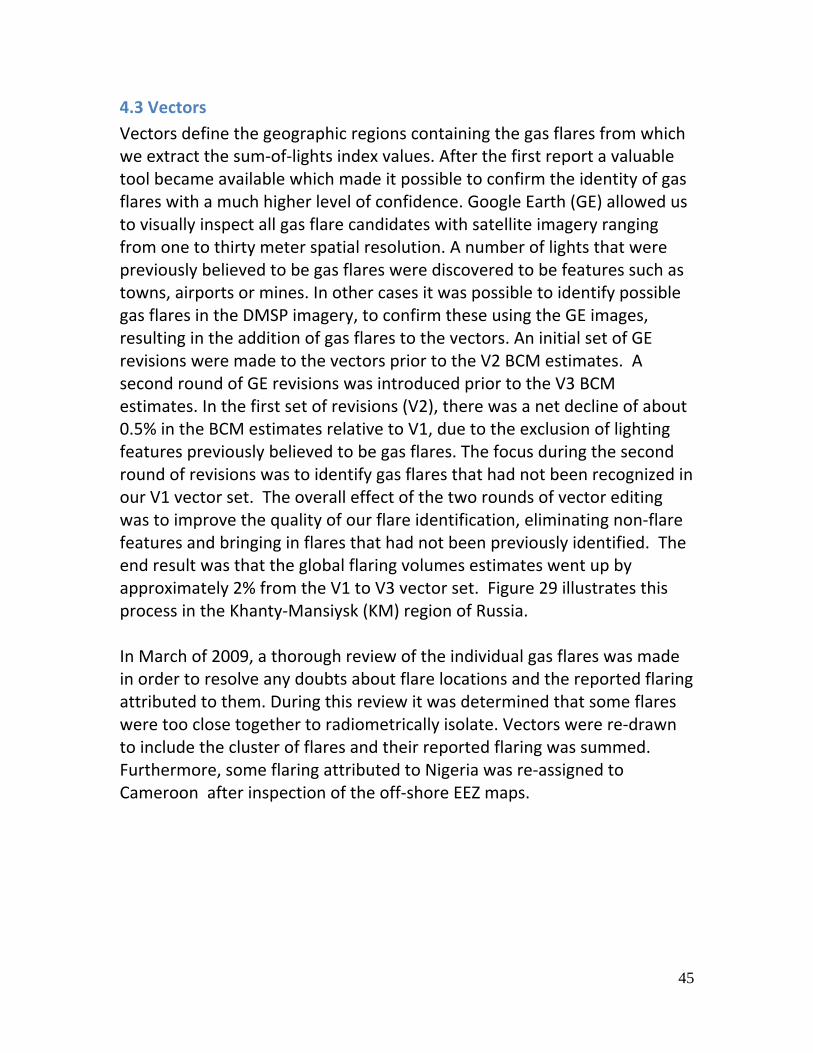
Vectors define the geographic regions containing the gas flares from which we extract the sum‐of‐lights index values. After the first report a valuable tool became available which made it possible to confirm the identity of gas flares with a much higher level of confidence. Google Earth (GE) allowed us to visually inspect all gas flare candidates with satellite imagery ranging from one to thirty meter spatial resolution. A number of lights that were previously believed to be gas flares were discovered to be features such as towns, airports or mines. In other cases it was possible to identify possible gas flares in the DMSP imagery, to confirm these using the GE images, resulting in the addition of gas flares to the vectors. An initial set of GE revisions were made to the vectors prior to the V2 BCM estimates. A second round of GE revisions was introduced prior to the V3 BCM estimates. In the first set of revisions (V2), there was a net decline of about 0.5% in the BCM estimates relative to V1, due to the exclusion of lighting features previously believed to be gas flares. The focus during the second round of revisions was to identify gas flares that had not been recognized in our V1 vector set. The overall effect of the two rounds of vector editing was to improve the quality of our flare identification, eliminating non‐flare features and bringing in flares that had not been previously identified. The end result was that the global flaring volumes estimates went up by approximately 2% from the V1 to V3 vector set. Figure 29 illustrates this process in the Khanty‐Mansiysk (KM) region of Russia. In March of 2009, a thorough review of the individual gas flares was made in order to resolve any doubts about flare locations and the reported flaring attributed to them. During this review it was determined that some flares were too close together to radiometrically isolate. Vectors were re‐drawn to include the cluster of flares and their reported flaring was summed. Furthermore, some flaring attributed to Nigeria was re‐assigned to
Cameroon after inspection of the off‐shore EEZ maps.
46
Figure 29 – This is an example of the revised vectors drawn over a typical annual composite (F16 2004). The red vector is from the V1 set and the green is from V3. Note that both new flares are identified and counted and some lights are excluded because they were recognized as some other type of light.
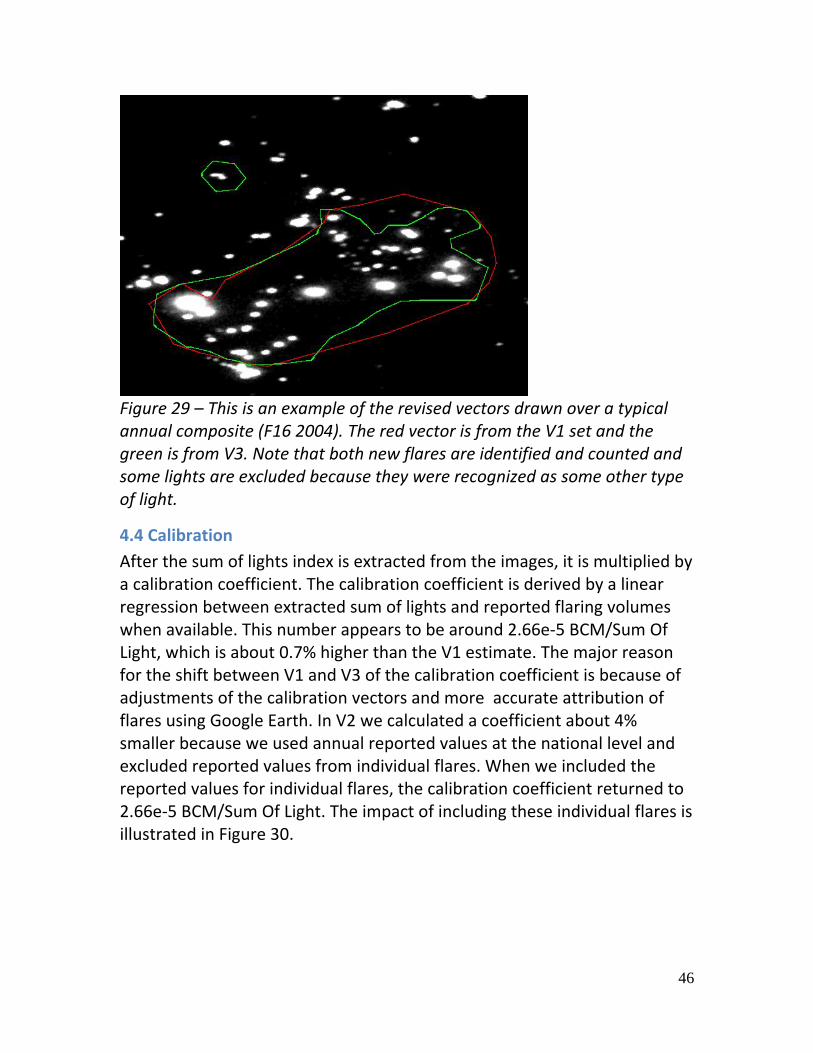
4.4 Calibration
After the sum of lights index is extracted from the images, it is multiplied by a calibration coefficient. The calibration coefficient is derived by a linear regression between extracted sum of lights and reported flaring volumes when available. This number appears to be around 2.66e‐5 BCM/Sum Of Light, which is about 0.7% higher than the V1 estimate. The major reason for the shift between V1 and V3 of the calibration coefficient is because of adjustments of the calibration vectors and more accurate attribution of flares using Google Earth. In V2 we calculated a coefficient about 4% smaller because we used annual reported values at the national level and excluded reported values from individual flares. When we included the reported values for individual flares, the calibration coefficient returned to 2.66e‐5 BCM/Sum Of Light. The impact of including these individual flares is illustrated in Figure 30.
47
Figure 30 – The calibration coefficient is derived by linear regression. The first plot shows all the calibration data. The second plot is a close‐up near the origin showing how the inclusion of individual flares can shift the value of the calibration coefficient. The initial report (V1), the 2008 revision (V2), and this current estimate (V3) each have differences from each other that lead to differences in global estimates. Table 6 summarizes these differences in estimated global flaring (in % difference of BCM from V1):
48
TABLE 6
Estimate Input Data Vectors Calibration Net Average Difference from V1 of global estimated flaring
V1 May 17, 2007
2006 was represented by a partial year from satellite F15 and 2005 included only data from F15.
Original set. 2.646e‐5
V2 October 30, 2008
The precision of our summation software improved, which increased estimates of flare volumes by 1.5% over V1. F16 was added for 2005‐2007. F15 2005 was reprocessed and F15 2006 was replaced with a full year.
Google Earth was used to eliminate lights due to other sources and add gas flares in some cases. Net decrease of 0.5% in global flared BCM.
2.57e‐5 based on country data only (reported data from individual gas flares excluded). Net decrease of about 3% in global flared BCM.
2% decrease
V3 March, 2009
Data was extended to include two satellites in both 2007 and 2008. Intercalibration and code improvements remained the same as V2.
More gas flares were identified based on Google Earth. Net increase of 2% in global flared BCM.
2.66e‐5 based on full set of reported BCM values and more accurate attribution of flares, an increase of 0.7%
4% increase
49
5. Conclusion
This report extends the estimation of global gas flaring volumes to include 2007 and 2008. The results indicate that gas flaring peaked at about 172 BCM in 2005 and has declined by 34 BCM down to 138 BCM by 2008. We document some of the improvements made in gas flare identification using Google Earth imagery. Both additional flares were detected and previously suspected lights were disqualified. Google Earth has proven to be an invaluable resource in the identification and confirmation of flares. NGDC is rapidly converging on an improved method of intercalibrating the observations by different satellites. It is based on the moonlight being reflected off of homogenous bright desert surfaces (i.e. White Sands, NM). This geo‐physical approach will not be dependent on unverifiable assumptions based on anthropogenic lighting. A study of environmental effects suggests that snow cover is probably negligible in its contribution to gas flare volume estimates. However, gas flares on water appear systematically dimmer than those on land for the same reported volume of gas burned. This is consistent with the hypothesis that the surrounding water absorbs more of the Near‐IR radiation than land. A method for accounting for this environmental effect was devised and is being tested for operational use. A multi‐faceted study of the effects of saturated pixels on the estimated gas flaring volumes was performed. The tentative conclusion is that saturation does not significantly bias the results. Because of this finding, this report does not include any correction for saturation. In conclusion, during the second year of research we were able to expand on the methods developed to estimate gas flaring using satellite observations and extend the record through 2008. We were also able to identify areas which could significantly improve the accuracy of our retrievals through better intercalibration between satellites and more sophisticated treatment of saturated pixels. Progress is being made on these enhancements.
50
References
Che, N and JC Price, "Improved method for calibrating the visible and near‐
infrared channels of the National Oceanic and Atmospheric Administration Advanced Very High Resolution Radiometer," Appl. Opt. 32, 7471‐7478 (1993).
Elvidge, CD, KE Baugh, BJ Tuttle, AT Howard, DW Pack, C Milesi, EH Erwin,
2007, A Twelve Year Record of National and Global Gas Flaring Volumes Estimated Using Satellite Data, Report to the World Bank.
Gallegos,S., RE Ryan, R Baud, JM Bloemker, 2007, MODIS Products to
Improve the Monitoring of Gas Flaring From Offshore Oil and gas Facilities. Final Report to NASA, 10 pages.
Janiczek, PM, JA DeYoung, 1987, Computer Programs for Sun and Moon
Illuminance with Contingent Tables and Diagrams, United States Naval Observatory, Circular No. 171.
Orr, MJL, 1999, Matlab Functions for Radial Basis Function Networks,
Technical Report, Institute for Adaptive and Neural Computation, Division of Informatics, Edinburgh University.
51
APPENDIX A ‐ Does Pixel Saturation Matter? To jump right to the conclusion, after exploring an array of methods to reduce the effect of saturated pixels, the estimate of gas flaring remains surprisingly robust. This leads to the conclusion that saturated pixels are far less of a concern than previously believed.
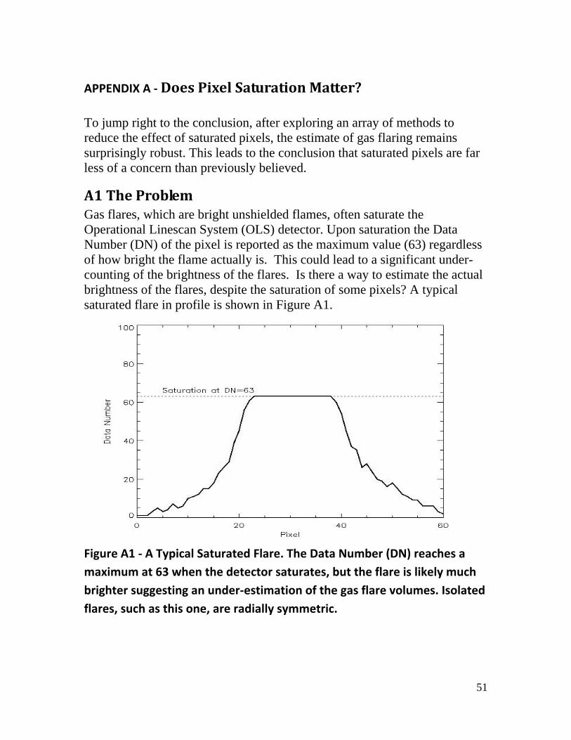
A1 The Problem Gas flares, which are bright unshielded flames, often saturate the Operational Linescan System (OLS) detector. Upon saturation the Data Number (DN) of the pixel is reported as the maximum value (63) regardless of how bright the flame actually is. This could lead to a significant under-counting of the brightness of the flares. Is there a way to estimate the actual brightness of the flares, despite the saturation of some pixels? A typical saturated flare in profile is shown in Figure A1.
Figure A1 ‐ A Typical Saturated Flare. The Data Number (DN) reaches a
maximum at 63 when the detector saturates, but the flare is likely much
brighter suggesting an under‐estimation of the gas flare volumes. Isolated
flares, such as this one, are radially symmetric.
52
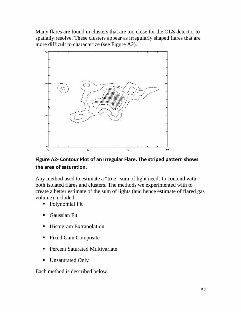
Many flares are found in clusters that are too close for the OLS detector to spatially resolve. These clusters appear as irregularly shaped flares that are more difficult to characterize (see Figure A2).
Figure A2‐ Contour Plot of an Irregular Flare. The striped pattern shows
the area of saturation.
Any method used to estimate a “true” sum of light needs to contend with both isolated flares and clusters. The methods we experimented with to create a better estimate of the sum of lights (and hence estimate of flared gas volume) included: Polynomial Fit
Gaussian Fit
Histogram Extrapolation
Fixed Gain Composite
Percent Saturated Multivariate
Unsaturated Only
Each method is described below.
53
A2 The Polynomial Fit The shoulders of a saturated flare suggest that it could be fitted by a polynomial function. This Polynomial Fit method would fit the shape of the each flare with a function that would estimate what the peak values would have been had the detector remained unsaturated (see Figure A3).
Figure A3 ‐ A Saturated Flare (solid) and a 4th Order Polynomial Fit
(dashed). The horizontal line shows where saturation occurs (DN=63).
When this method encounters a broad flare, the “best fit” is not always the choice our intuition would select to complete the curve in the saturated region (see Figure A4). And another complication arises when we consider that many flares are irregularly shaped (e.g. Figure A2), so there is no single transect that appropriately describes the shape of the flare to be fit.
54
Figure A4 ‐ A Broad Flare. The 4th order Polynomial Fit (dashed line) does
not overshoot the saturation value, as would be expected by a flare of
this size. The Polynomial Fit is probably a significant under‐estimation of
the flare's brightness.
A3 The Gaussian Fit Approach Rather than attempt to fit all flare shapes (both nearly circular and irregularly shaped) with similar polynomial or Gaussian functions, an alternate approach was developed. In this approach, for each saturated region we counted the number of saturated pixels (N). Then we treated them as if they were a circular and symmetric form of area N. From this stipulation a radius (R) can be calculated,
R = (N/π)1/2. Next we assume the saturated region follows the shape of a Gaussian curve, such that the height of the flare (y), as a function of its distance from a central point (r) is described as:
55
y = P exp(-z2/2), where z = r/d.
The decay value of the flare (d) represents how quickly the Gaussian function decays from its peak. A large value creates a broad slowly falling curve, whereas a small value of d creates a sharp function. P is the peak value of the Gaussian at the central point (r=0). We can then solve for P for any R by setting the value of y to the saturation DN value of 63:
63 = P exp(-(R/d)2/2), or P = 63 exp((R/d)2/2)
With an analytic function describing the peak DN of the flare, we can integrate to estimate the volume (V) of the uncounted peak above saturation:
V = ∫P exp(-(r/d)2/2) dV
This integration is performed for the volume of the modeled flare where its value is 63 and larger. The volume is later added to the N saturated pixels (DN=63) and the unsaturated sum of lights (i.e. the flanks of the flare). The solution of the integral is:
V = 2πd2(P – 63 + 63 ln(63/P))
V is the additional signal that would have been detected if saturation had not occurred. Therefore the corrected sum of lights (L) is:
L = N * 63 + V + Lunsat,
where Lunsat is the sum of lights of the unsaturated pixels in the flanks around the saturated region.
What value of d should be used? Although, d=2 resembles an isolated flare, when this value was used to estimate the uncounted flare amounts it led to an unrealistically high correction (see Figure A5). This is because so many saturated flares occur in clusters. An empirical search found that d=13 provided the best fit of the reported flaring data. However, d=13 converges to essentially no correction for any but the largest flare clusters.
56
Figure A5 ‐ Gaussian forms to fit flares of 20 saturated pixels with varying
decay factor (d).
A4 The FixedGain Composite Method On several periods during the year, the US Air Force will comply with our request to reduce the gain of the Operational Linescan System (OLS) to collect what we refer to as “fixed-gain” data. The gain is set to 15, 35, or 55. When the gain is set to 55, it approximately corresponds to the sensitivity of the operational mode. The gain of 35 decreases the sensitivity by a factor of 10. Likewise, 15 is a factor of 100 less sensitive than the operational mode. When the gain is set to 15, only the brightest objects such as city centers and gas flares are visible and almost no pixels are saturated. By combining all the fixed-gain data over a thirteen month period we created a composite that is appropriately scaled to include only unsaturated data. This product is referred to as the “Fixed-Gain Composite”. This product was used to create an estimate of the average value of saturated pixels (see Fig A6).
57
Figure A6 ‐ An Estimate of the Data Number of a Saturated Pixel. The
Fixed Gain Composite was masked to include only saturated pixels as seen
in the annual average (variable gain) images. Then the sum of lights was
computed. The regression line shows a slope of 707 per saturated pixel.
Using this derived factor from the fixed gain data we were able to formulate the Sum of Lights (L) from the variable gain (i.e. operational) mode as:
L = N * 707 + Lunsat, where Lunsat is the sum of lights of the unsaturated pixels within that region, and N is the number of saturated pixels. Some saturated pixels would probably have the value of 65 (i.e. only slightly higher than the saturation value). Whereas other pixels had a measured value of several thousand using the fixed gain composite. The value of 707 represents the average contribution of a saturated pixel.
58
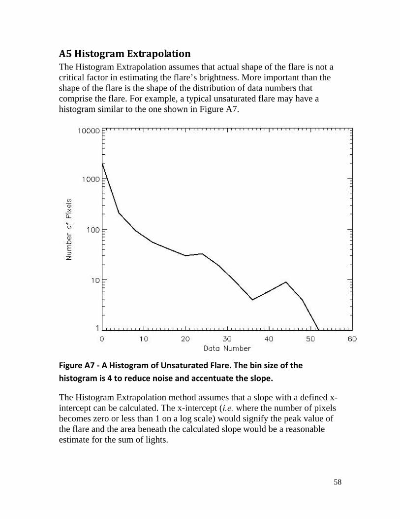
A5 Histogram Extrapolation The Histogram Extrapolation assumes that actual shape of the flare is not a critical factor in estimating the flare’s brightness. More important than the shape of the flare is the shape of the distribution of data numbers that comprise the flare. For example, a typical unsaturated flare may have a histogram similar to the one shown in Figure A7.
Figure A7 ‐ A Histogram of Unsaturated Flare. The bin size of the
histogram is 4 to reduce noise and accentuate the slope.
The Histogram Extrapolation method assumes that a slope with a defined x-intercept can be calculated. The x-intercept (i.e. where the number of pixels becomes zero or less than 1 on a log scale) would signify the peak value of the flare and the area beneath the calculated slope would be a reasonable estimate for the sum of lights.
59
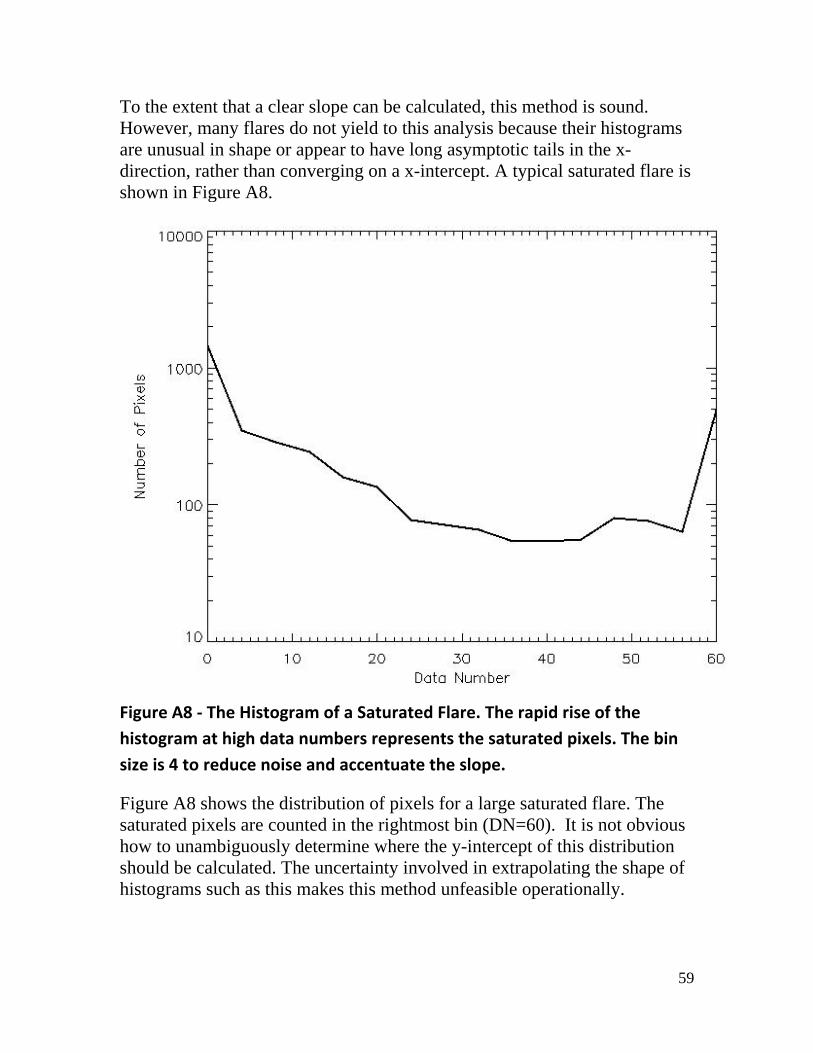
To the extent that a clear slope can be calculated, this method is sound. However, many flares do not yield to this analysis because their histograms are unusual in shape or appear to have long asymptotic tails in the x-direction, rather than converging on a x-intercept. A typical saturated flare is shown in Figure A8.
Figure A8 ‐ The Histogram of a Saturated Flare. The rapid rise of the
histogram at high data numbers represents the saturated pixels. The bin
size is 4 to reduce noise and accentuate the slope.
Figure A8 shows the distribution of pixels for a large saturated flare. The saturated pixels are counted in the rightmost bin (DN=60). It is not obvious how to unambiguously determine where the y-intercept of this distribution should be calculated. The uncertainty involved in extrapolating the shape of histograms such as this makes this method unfeasible operationally.
60
A6 Percent Saturated Multivariate In order to avoid the effects of saturation, the extraction is run twice. The first is the usual method which allows saturated data to be averaged in with non-saturated data. The second run excludes all saturated pixels from the creation of the annual averages. To distinguish these two runs we use a subscript of 62 to denote that saturated pixels were excluded. No subscript denotes the standard annual product (which contains saturated data averaged with non-saturated data). Now we have two decoupled parameters to perform a regression against, the unsaturated sum of lights (L62) and the percent saturation (Psat). We define Psat as:
Psat =100 * (U – U62)/N U is the light from the ordinary annual composite for a given pixel and U62 is the light with all saturated pixels excluded when the annual composite is generated. N is the number of pixels contributing to that composite in the ordinary case. We cast the new equation as:
F = a0 L62 + a1 Psat where F is the estimated flared volume in Billion Cubic Meters (BCM), L62 is the sum of lights of the unsaturated data (DN from 0 to 62). A constant term was added to the regression, but it was found to be negligible except it added a bias for regions of no flaring. Later it was dropped from the analysis. The value of this approach is that it decouples the actual DN of the saturated pixels and allows them to be fitted by a1. The result was a value of a0 (the coefficient of the unsaturated sum of lights) significantly higher than standard calibrations because L62 is always smaller than L. The value of a1 was surprisingly negative, serving as a “correction” to the high gas flaring volume estimate. Furthermore, the magnitude of a1 was small, so that the effect of adding this second parameter was marginal except for areas with very high frequency of pixel saturation (e.g. Nigeria).
61
A7 Using Unsaturated Data Only Our experience with the multivariate method suggested that sufficient information regarding the brightness of the flare was contained in the unsaturated shoulders, rather than in the saturated core. Could our analysis be realistically performed by excluding all saturated data?
F = a0 L62,
where F is the gas flaring volume, L62 is the unsaturated sum of lights, and a0 is the fitted parameter based on calibration data. The unsaturated-only method provided results that were consistent with the other methods.
A8 Results The results of each method are presented in Table 1 and graphically in Figure A9. Table 1 – Global Gas Flaring estimates by Various Methods to Correct for Saturation. An explanation of each column is provided in Table 2. YEAR WB2007 AMS2008 D5 D13 MV N707 C62
Table 2 – An Explanation of the Columns of Table 1. Some methods are not included because they were investigated in an experimental fashion and not used to estimate global flaring.
62
Column Description Calibration Coefficient [BCM/SOL x 10-5]
WB2007 World Bank 2007 Report 2.646AMS2008 AMSTERDAM Meeting Dec 2008 2.57
D13 Method of correcting for saturation, Decay Factor = 13 2.63
D5 Method of correcting for saturation, Decay Factor = 5 2.38
MV Multivariate calibration involving both SOL and Nsaturated 4.6
N707 Adding a factor (707) for each Saturated pixel, based on the Unsaturated composite 1.6
C62 Unsaturated data only 3.23
Figure A9 ‐ Global Gas Flaring Volumes.
A10 Conclusion There is a strong convergence around a robust estimate of the global gas flaring volume regardless of the method used to correct for pixel saturation (including no correction at all). The simplest conclusion to draw from this observation is that pixel saturation does not significantly bias the estimated gas flaring volume. There are several possible explanations to support this unexpected conclusion:
The calibration dataset includes 'saturated' data to approximately the same extent as the rest of the data, and therefore the calibration
63
coefficient obtained approximately corrects for under-estimation of saturated flares.
Saturated regions account for about 15% of the actual sum of lights. Most of the information is contained in the unsaturated regions surrounding the saturated pixels.
When the sum of lights from Fixed Gain data, which contains no saturated pixels, is plotted against the 'normal gain' data which includes saturated pixels, the relationship is linear at all scales (see Figure A10). If saturation were affecting the sum of lights calculated from the 'standard gain' data significantly, then regions of high saturation would be expected to cause a “bend” in the data.
Figure A10 ‐ Sum of Lights computed from Fixed Gain data and the
Standard (variable gain) Method. Note the linearity for even the highest
flaring countries.
64
APPENDIX B
A Fifteen Year Record of Global Natural Gas Flaring Derived from Satellite Data, Energies v. 2, p. 595-622.